fourier Analysis For Vectors - Universitetet i Oslo · Fourier analysis for vectors ... MATLAB...
53
Chapter 3 Fourier analysis for vectors In Chapter 2 we saw how a function defined on an interval can be decomposed into a linear combination of sines and cosines, or equivalently, a linear combi- nation of complex exponential functions. However, this kind of decomposition is not very convenient from a computational point of view. The coefficients are given by integrals that in most cases cannot be evaluated exactly, so some kind of numerical integration technique would have to be applied. In this chapter our starting point is simply a vector of finite dimension. Our aim is then to decompose this vector in terms of linear combinations of vectors built from complex exponentials. This simply amounts to multiplying the original vector by a matrix, and there are efficient algorithms for doing this. It turns out that these algorithms can also be used for computing good approximations to the continuous Fourier series in Chapter 2. Recall from Chapter 1 that a digital sound is simply a sequence of num- bers, in other words, a vector. An algorithm for decomposing a vector into combinations of complex exponentials therefore corresponds to an algorithm for decomposing a digital sound into a combination of pure tones. 3.1 Basic ideas We start by recalling what a digital sound is and by establishing some notation and terminology. Fact 3.1. A digital sound is a finite sequence (or equivalently a vector) x of numbers, together with a number (usually an integer) f s , the sample rate, which denotes the number of measurements of the sound per second. The length of the vector is usually assumed to be N , and it is indexed from 0 to N − 1. Sample k is denoted by x k , i.e., x =(x k ) N−1 k=0 . 55
Transcript of fourier Analysis For Vectors - Universitetet i Oslo · Fourier analysis for vectors ... MATLAB...
Chapter 3
Fourier analysis for vectors
In Chapter 2 we saw how a function defined on an interval can be decomposedinto a linear combination of sines and cosines, or equivalently, a linear combi-nation of complex exponential functions. However, this kind of decompositionis not very convenient from a computational point of view. The coefficients aregiven by integrals that in most cases cannot be evaluated exactly, so some kindof numerical integration technique would have to be applied.
In this chapter our starting point is simply a vector of finite dimension.Our aim is then to decompose this vector in terms of linear combinations ofvectors built from complex exponentials. This simply amounts to multiplyingthe original vector by a matrix, and there are efficient algorithms for doingthis. It turns out that these algorithms can also be used for computing goodapproximations to the continuous Fourier series in Chapter 2.
Recall from Chapter 1 that a digital sound is simply a sequence of num-bers, in other words, a vector. An algorithm for decomposing a vector intocombinations of complex exponentials therefore corresponds to an algorithm fordecomposing a digital sound into a combination of pure tones.
3.1 Basic ideas
We start by recalling what a digital sound is and by establishing some notationand terminology.
Fact 3.1. A digital sound is a finite sequence (or equivalently a vector) x
of numbers, together with a number (usually an integer) fs, the sample rate,which denotes the number of measurements of the sound per second. Thelength of the vector is usually assumed to be N , and it is indexed from 0 toN − 1. Sample k is denoted by xk, i.e.,
x = (xk)N−1k=0 .
55

Note that this indexing convention for vectors is not standard in mathe-matics and is different from what we have used before. Note in particular thatMATLAB indexes vectors from 1, so algorithms given here must be adjustedappropriately.
We also need the standard inner product and norm for complex vectors. Atthe outset our vectors will have real components, but we are going to performFourier analysis with complex exponentials which will often result in complexvectors.
Definition 3.2. For complex vectors of length N the Euclidean inner productis given by
�x,y� =N−1�
k=0
xkyk. (3.1)
The associated norm is
�x� =
����N−1�
k=0
|xk|2. (3.2)
In the previous chapter we saw that, using a Fourier series, a function withperiod T could be approximated by linear combinations of the functions (thepure tones) {e2πint/T }N
n=0. This can be generalised to vectors (digital sounds),but then the pure tones must of course also be vectors.
Definition 3.3 (Fourier analysis for vectors). In Fourier analysis of vectors,a vector x = (x0, . . . , xN−1) is represented as a linear combination of the Nvectors
φn=
1√N
�1, e2πin/N , e2πi2n/N , . . . , e2πikn/N , . . . , e2πin(N−1)/N
�.
These vectors are called the normalised complex exponentials or the pure digi-tal tones of order N . The whole collection FN = {φ
n}Nn=0 is called the N -point
Fourier basis.
The following lemma shows that the vectors in the Fourier basis are orthog-onal, so they do indeed form a basis.
Lemma 3.4. The normalised complex exponentials {φn}N−1n=0 of order N form
an orthonormal basis in RN .
Proof. Let n1 and n2 be two distinct integers in the range [0, N − 1]. The inner
56

product of φn1
and φn2
is then given by
N�φn1,φ
n2� = �e2πin1k/N , e2πin2k/N �
=N−1�
k=0
e2πin1k/Ne−2πin2k/N
=N−1�
k=0
e2πi(n1−n2)k/N
=1− e2πi(n1−n2)
1− e2πi(n1−n2)/N
= 0.
In particular, this orthogonality means that the the complex exponentials forma basis. And since we also have �φ
n,φ
n� = 1 it is in fact an orthonormal
basis.
Note that the normalising factor 1√N
was not present for pure tones in theprevious chapter. Also, the normalising factor 1
Tfrom the last chapter is not
part of the definition of the inner product in this chapter. These are smalldifferences which have to do with slightly different notation for functions andvectors, and which will not cause confusion in what follows.
3.2 The Discrete Fourier Transform
Fourier analysis for finite vectors is focused around mapping a given vectorfrom the standard basis to the Fourier basis, performing some operations on theFourier representation, and then changing the result back to the standard basis.The Fourier matrix, which represents this change of basis, is therefore of crucialimportance, and in this section we study some of its basic properties. We startby defining the Fourier matrix.
Definition 3.5 (Discrete Fourier Transform). The change of coordinates fromthe standard basis of RN to the Fourier basis FN is called the discrete Fouriertransform (or DFT). The N×N matrix FN that represents this change of basisis called the (N -point) Fourier matrix. If x is a vector in RN , its coordinatesy = (y0, y1, . . . , yN−1) relative to the Fourier basis are called the Fourier coef-ficients of x, in other words y = FNx). The DFT of x is sometimes denotedby x̂.
We will normally write x for the given vector in RN , and y for the DFT ofthis vector. In applied fields, the Fourier basis vectors are also called synthesisvectors, since they can be used used to “synthesize” the vector x, with weightsprovided by the DFT coefficients y = (yn)
N−1n=0 . To be more precise, we have
57

that the change of coordinates performed by the DFT can be written as
x = y0φ0 + y1φ1 + · · ·+ yN−1φN−1 =�φ0 φ1 · · · φ
N−1
�y = F−1
Ny, (3.3)
where we have used the inverse of the defining relation y = FNx, and that theφ
nare the columns in F−1
N(this follows from the fact that F−1
Nis the change
of coordinates matrix from the Fourier basis to the standard basis, and theFourier basis vectors are clearly the columns in this matrix). Equation (3.3) isalso called the synthesis equation.
Let us also find the matrix FN itself. From Lemma 3.4 we know that thecolumns of F−1
Nare orthonormal. If the matrix was real, it would have been
called orthogonal, and the inverse matrix could be obtained by transposing. F−1N
is complex however, and it is easy to see that the conjugation present in thedefinition of the inner product (3.1) translates into that the inverse of a complexmatrix with orthonormal columns is given by the matrix where the entries areboth transposed and conjugated. Let us denote the conjugated transpose of Tby TH , and say that a complex matrix is unitary when T−1 = TH . From ourdiscussion it is clear that F−1
Nis a unitary matrix, i.e. its inverse, FN , is its
conjugate transpose. Moreover since F−1N
is symmetric, its inverse is in fact justits conjugate,
FN = F−1N
.
Theorem 3.6. The Fourier matrix FN is the unitary N × N -matrix withentries given by
(FN )nk =1√N
e−2πink/N ,
for 0 ≤ n, k ≤ N − 1.
Note that in the signal processing literature, it is not common to includethe normalizing factor 1/
√N in the definition of the DFT. From our more
mathematical point of view this is useful since it makes the Fourier matrixunitary.
In practical applications of Fourier analysis one typically applies the DFT,performs some operations on the coefficients, and then maps the result backusing the inverse Fourier matrix. This inverse transformation is so commonthat it deserves a name of its own.
Definition 3.7 (IDFT). If y ∈ RN the vector x = (FN )Hy is referred to asthe inverse discrete Fourier transform or (IDFT) of y.
That y is the DFT of x and x is the IDFT of y can also be expressed in
58

component form
xk =1√N
N−1�
n=0
yne2πink/N , (3.4)
yn =1√N
N−1�
k=0
xke−2πink/N . (3.5)
In applied fields such as signal processing, it is more common to state theDFT and IDFT in these component forms, rather than in the matrix formsx = (FN )Hy and y = FNy.
Let us use now see how these formulas work out in practice by consideringsome examples.
Example 3.8 (DFT on a square wave). Let us attempt to apply the DFT toa signal x which is 1 on indices close to 0, and 0 elsewhere. Assume that
x−L = . . . = x−1 = x0 = x1 = . . . = xL = 1,
while all other values are 0. This is similar to a square wave, with some mod-ifications: First of all we assume symmetry around 0, while the square waveof Example 1.11 assumes antisymmetry around 0. Secondly the values of thesquare wave are now 0 and 1, contrary to −1 and 1 before. Finally, we have adifferent proportion of where the two values are assumed. Nevertheless, we willalso refer to the current digital sound as a square wave.
Since indices with the DFT are between 0 an N−1, and since x is assumed tohave period N , the indices [−L,L] where our signal is 1 translates to the indices[0, L] and [N − L,N − 1] (i.e., it is 1 on the first and last parts of the vector).Elsewhere our signal is zero. Since
�N−1k=N−L
e−2πink/N =�−1
k=−Le−2πink/N
(since e−2πink/N is periodic with period N), the DFT of x is
yn =1√N
L�
k=0
e−2πink/N +1√N
N−1�
k=N−L
e−2πink/N
=1√N
L�
k=0
e−2πink/N +1√N
−1�
k=−L
e−2πink/N
=1√N
L�
k=−L
e−2πink/N
=1√N
e2πinL/N1− e−2πin(2L+1)/N
1− e−2πin/N
=1√N
e2πinL/Ne−πin(2L+1)/Neπin/Neπin(2L+1)/N − e−πin(2L+1)/N
eπin/N − e−πin/N
=1√N
sin(πn(2L+ 1)/N)
sin(πn/N).
59
This computation does in fact also give us the IDFT of the same vector, sincethe IDFT just requires a change of sign in all the exponents. From this examplewe see that, in order to represent x in terms of frequency components, allcomponents are actually needed. The situation would have been easier if onlya few frequencies were needed.
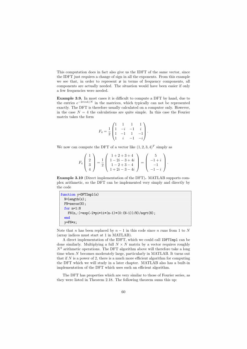
Example 3.9. In most cases it is difficult to compute a DFT by hand, due tothe entries e−2πink/N in the matrices, which typically can not be representedexactly. The DFT is therefore usually calculated on a computer only. However,in the case N = 4 the calculations are quite simple. In this case the Fouriermatrix takes the form
F4 =1
2
1 1 1 11 −i −1 i1 −1 1 −11 i −1 −i
.
We now can compute the DFT of a vector like (1, 2, 3, 4)T simply as
F4
1234
=1
2
1 + 2 + 3 + 41− 2i− 3 + 4i1− 2 + 3− 41 + 2i− 3− 4i
=
5−1 + i−1
−1− i
.
Example 3.10 (Direct implementation of the DFT). MATLAB supports com-plex arithmetic, so the DFT can be implemented very simply and directly bythe code
function y=DFTImpl(x)
N=length(x);
FN=zeros(N);
for n=1:N
FN(n,:)=exp(-2*pi*1i*(n-1)*(0:(N-1))/N)/sqrt(N);
end
y=FN*x;
Note that n has been replaced by n − 1 in this code since n runs from 1 to N(array indices must start at 1 in MATLAB).
A direct implementation of the IDFT, which we could call IDFTImpl can bedone similarly. Multiplying a full N × N matrix by a vector requires roughlyN2 arithmetic operations. The DFT algorithm above will therefore take a longtime when N becomes moderately large, particularly in MATLAB. It turns outthat if N is a power of 2, there is a much more efficient algorithm for computingthe DFT which we will study in a later chapter. MATLAB also has a built-inimplementation of the DFT which uses such an efficient algorithm.
The DFT has properties which are very similar to those of Fourier series, asthey were listed in Theorem 2.18. The following theorem sums this up:
60

Theorem 3.11 (DFT properties). Let x be a real vector of length N . TheDFT has the following properties:
1. (�x)N−n
= (�x)n
for 0 ≤ n ≤ N − 1.
2. If z is the vector with the components of x reversed so that zk = xN−k
for 0 ≤ k ≤ N − 1, then �z = �x. In particular,
(a) if xk = xN−k for all n (so x is symmetric), then �x is a real vector.(b) if xk = −xN−k for all k (so x is antisymmetric), then �x is a purely
imaginary vector.
3. If d is an integer and z is the vector with components zk = xk−d (thevector x with its elements delayed by d), then (�z)
n= e−2πidn/N (�x)
n.
4. If d is an integer and z is the vector with components zk = e2πidk/Nxk,then (�z)
n= (�x)
n−d.
5. Let d be a multiple of 1/2. Then the following are equivalent:
(a) xd+k = xd−k for all k so that d+ k and d− k are integers (in otherwords x is symmetric about d).
(b) The argument of (�x)n
is −2πdn/N for all n.
Proof. The methods used in the proof are very similar to those used in the proofof Theorem 2.18. From the definition of the DFT we have
(�x)N−n
=1√N
N−1�
k=0
e−2πik(N−n)/Nxk =1√N
N−1�
k=0
e2πikn/Nxk
=1√N
N−1�
k=0
e−2πikn/Nxk = (�x)n
which proves property 1. To prove property 2, we write
(�z)n=
1√N
N−1�
k=0
zke−2πikn/N =
1√N
N−1�
k=0
xN−ke−2πikn/N
=1√N
N�
u=1
xue−2πi(N−u)n/N =
1√N
N−1�
u=0
xue2πiun/N
=1√N
N−1�
u=0
xue−2πiun/N = (�x)n.
If x is symmetric it follows that z = x, so that (�x)n= (�x)
n. Therefore x must
be real. The case of antisymmetry follows similarly.
61
To prove property 3 we observe that
(�z)n=
1√N
N−1�
k=0
xk−de−2πikn/N =
1√N
N−1�
k=0
xke−2πi(k+d)n/N
= e−2πidn/N 1√N
N−1�
k=0
xke−2πikn/N = e−2πidn/N (�x)
n.
For the proof of property 4 we note that the DFT of z is
(�z)n=
1√N
N−1�
k=0
e2πidk/Nxne−2πikn/N =
1√N
N−1�
k=0
xne−2πi(n−d)k/N = (�x)
n−d.
Finally, to prove property 5, we note that if d is an integer, the vector z
where x is delayed by −d samples satisfies the relation (�z)n= e2πidn/N (�x)
n
because of property 3. Since z satisfies zn = zN−n, we have by property 2that (�z)
nis real, and it follows that the argument of (�x)
nis −2πdn/N . It is
straightforward to convince oneself that property 5 also holds when d is not aninteger also (i.e., a multiple of 1/2).
For real sequences, Property 1 says that we need to store only about one halfof the DFT coefficients, since the remaining coefficients can be obtained by con-jugation. In particular, when N is even, we only need to store y0, y1, . . . , yN/2,since the other coefficients can be obtained by conjugating these.
3.2.1 Connection between the DFT and Fourier series
So far we have focused on the DFT as a tool to rewrite a vector in terms ofdigital, pure tones. In practice, the given vector x will often be sampled fromsome real data given by a function f(t). We may then talk about the frequencycontent of the vector x and the frequency content of f and ask ourselves howthese are related. More precisely, what is the relationship between the Fouriercoefficients of f and the DFT of x?
In order to study this, assume for simplicity that f is a sum of finitely manyfrequencies. This means that there exists an M so that f is equal to its Fourierapproximation fM ,
f(t) = fM (t) =M�
n=−M
zne2πint/T , (3.6)
where zn is given by
zn =1
T
�T
0f(t)e−2πint/T dt.
We recall that in order to represent the frequency n/T fully, we need the cor-responding exponentials with both positive and negative arguments, i.e., bothe2πint/T and e−2πint/T .
62
Fact 3.12. Suppose f is given by its Fourier series (3.6). Then the totalfrequency content for the frequency n/T is given by the two coefficients znand z−n.
Suppose that the vector x contains values sampled uniformly from f at Npoints,
xk = f(kT/N), for k = 0, 1, . . . , N − 1. (3.7)
The vector x can be expressed in terms of its DFT y as
xk =1√N
N−1�
n=0
yne2πink/N . (3.8)
If we evaluate f at the sample points we have
f(kT/N) =M�
n=−M
zne2πink/N , (3.9)
and a comparison now gives
M�
n=−M
zne2πink/N =
1√N
N−1�
n=0
yne2πink/N for k = 0, 1, . . . , N − 1.
Exploiting the fact that both y and the complex exponentials are periodic withperiod N , and assuming that we take N samples with N odd, we can rewritethis as
M�
n=−M
zne2πink/N =
1√N
(N−1)/2�
n=−(N−1)/2
yne2πink/N .
This is a matrix relation on the form Gz = Hy/√N , where
1. G is the N × (2M + 1)-matrix with entries 1√Ne2πink/N ,
2. H is the N ×N -matrix with entries 1√Ne2πink/N .
In Exercise 6 you will be asked to show that GHG = I2M+1, and that GHH =�I 0
�, when N ≥ 2M + 1. Thus, if we choose the number of sample points
N so that N ≥ 2M + 1, multiplying with GH on both sides in Gz = Hy/√N
gives us that
z =�I 0
�� 1√N
y
�,
i.e. z consists of the first 2M + 1 elements in y/√N . Setting N = 2M + 1 we
can summarize this.
63
Proposition 3.13 (Relation between Fourier coefficients and DFT coeffi-cients). Let f be a Fourier series
f(t) =M�
n=−M
zne2πint/T ,
on the interval [0, T ] and let N = 2M + 1 be an odd integer. Suppose that x
is sampled from f by
xk = f(kT/N), for k = 0, 1, . . . , N − 1.
and let y be the DFT of x. Then z = y/√N , and the total contribution to f
from frequency n/T , where n is an integer in the range 0 ≤ n ≤ M , is givenby yn and yN−n.
We also need a remark on what we should interpret as high and low frequencycontributions, when we have applied a DFT. The low “frequency contribution”in f is the contribution from
e−2πiLt/T , . . . , e−2πit/T , 1, e2πit/T , . . . , e2πiLt/T
in f , i.e.�
L
n=−Lzne2πint/T . This means that low frequencies correspond to
indices n so that −L ≤ n ≤ L. However, since DFT coefficients have indicesbetween 0 and N − 1, low frequencies correspond to indices n in [0, L] ∪ [N −L,N − 1]. If we make the same argument for high frequencies, we see that theycorrespond to DFT indices near N/2:
Observation 3.14 (DFT indices for high and low frequencies). When y isthe DFT of x, the low frequencies in x correspond to the indices in y near 0and N . The high frequencies in x correspond to the indices in y near N/2.
We will use this observation in the following example, when we use the DFTto distinguish between high and low frequencies in a sound.
Example 3.15 (Using the DFT to adjust frequencies in sound). Since the DFTcoefficients represent the contribution in a sound at given frequencies, we canlisten to the different frequencies of a sound by adjusting the DFT coefficients.Let us first see how we can listen to the lower frequencies only. As explained,these correspond to DFT-indices n in [0, L]∪ [N −L,N −1]. In MATLAB thesehave indices from 1 to L+1, and from N−L+1 to N . The remaining frequencies,i.e. the higher frequencies which we want to eliminate, thus have MATLAB-indices between L + 2 and N − L. We can now perform a DFT, eliminatehigh frequencies by setting the corresponding frequencies to zero, and performan inverse DFT to recover the sound signal with these frequencies eliminated.With the help of the DFT implementation from Example 3.10, all this can beachieved with the following code:
64
y=DFTImpl(x);
y((L+2):(N-L))=zeros(N-(2*L+1),1);
newx=IDFTImpl(y);
To test this in practice, we also need to obtain the actual sound samples. Ifwe use our sample file castanets.wav, you will see that the code runs veryslowly. In fact it seems to never complete. The reason is that DFTImpl attemptsto construct a matrix FN with as many rows and columns as there are soundsamples in the file, and there are just too many samples, so that FN growstoo big, and matrix multiplication with it gets too time-consuming. We willshortly see much better strategies for applying the DFT to a sound file, but fornow we will simply attempt instead to split the sound file into smaller blocks,each of size N = 32, and perform the code above on each block. It turns outthat this is less time-consuming, since big matrices are avoided. You will bespared the details for actually splitting the sound file into blocks: you can findthe function playDFTlower(L) which performs this splitting, sets the relevantfrequency components to 0, and plays the resulting sound samples. If you trythis for L = 7 (i.e. we keep only 15 of the DFT coefficients) the result soundslike this. You can hear the disturbance in the sound, but we have not lost thatmuch even if more than half the DFT coefficients are dropped. If we instead tryL = 3 the result will sound like this. The quality is much poorer now. Howeverwe can still recognize the song, and this suggests that most of the frequencyinformation is contained in the lower frequencies.
Similarly we can listen to high frequencies by including only DFT coefficientswith index close to N
2 . The function playDFThigher(L) sets all DFT coefficientsto zero, except for those with indices N
2 − L, . . . , N
2 , . . . ,N
2 + L. Let us verifythat there is less information in the higher frequencies by trying the same valuesfor L as above for this function. For L = 7 (i.e. we keep only the middle 15DFT coefficients) the result sounds like this, for L = 3 the result sounds likethis. Both sounds are quite unrecognizable, confirming that most informationis contained in the lower frequencies.
Note that there may be a problem in the previous example: for each blockwe compute the frequency representation of the values in that block. But thefrequency representation may be different when we take all the samples intoconsideration. In other words, when we split into blocks, we can’t expect thatwe exactly eliminate all the frequencies in question. This is a common problemin signal processing theory, that one in practice needs to restrict to smallersegments of samples, but that this restriction may have undesired effects interms of the frequencies in the output.
3.2.2 Interpolation with the DFT
There are two other interesting facets to Theorem 3.13, besides connecting theDFT and the Fourier series: The first has to do with interpolation: The theo-rem enables us to find (unique) trigonometric functions which interpolate (pass
65
through) a set of data points. We have in elementary calculus courses seen howto determine a polynomial of degree N − 1 that interpolates a set of N datapoints — such polynomials are called interpolating polynomials. The followingresult tells how we can find an interpolating trigonometric function using theDFT.
Corollary 3.16 (Interpolation with the Fourier basis). Let f be a functiondefined on the interval [0, T ], and let x be the sampled sequence given by
xk = f(kT/N) for k = 0, 1, . . . , N − 1.
There is exactly one linear combination g(t) on the form
g(t) =1√N
N−1�
n=0
yne2πint/T
which satisfies the conditions
g(kT/N) = f(kT/N), k = 0, 1, . . . , N − 1
and its coefficients are determined by the DFT y = x̂ of x.
The proof for this follows by inserting t = 0, t = T/N , t = 2T/N , . . . ,t = (N − 1)T/N in the equation f(t) = 1√
N
�N−1n=0 yne2πint/T to arrive at the
equations
f(kT/N) =1√N
N−1�
n=0
yne2πink/N 0 ≤ k ≤ N − 1.
This gives us an equation system for finding the yn with the invertible Fouriermatrix as coefficient matrix, and the result follows.
3.2.3 Sampling and reconstruction with the DFT
The second interesting facet to Theorem 3.13 has to do with when reconstructionof a function from its sample values is possible. An example of sampling afunction is illustrated in Figure 3.1. From Figure 3.1(b) it is clear that someinformation is lost when we discard everything but the sample values. Theremay however be an exception to this, if we assume that the function satisfiessome property. Assume that f is equal to a finite Fourier series. This meansthat f can be written on the form (3.6), so that the highest frequency in thesignal is bounded by M/T . Such functions also have their own name:
Definition 3.17 (Band-limited functions). A function f is said to be band-limited if there exists a number ν so that f does not contain frequencies higherthan ν.
66
0.2 0.4 0.6 0.8 1.0
�1.0
�0.5
0.5
1.0
(a)
0.2 0.4 0.6 0.8 1.0
�1.0
�0.5
0.5
1.0
(b)
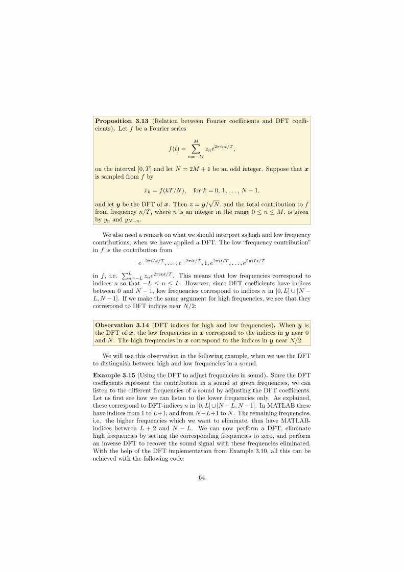
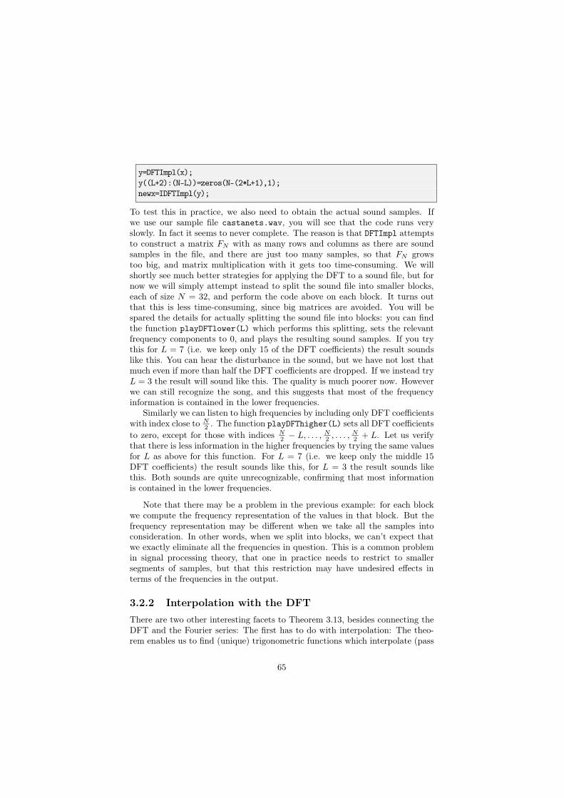
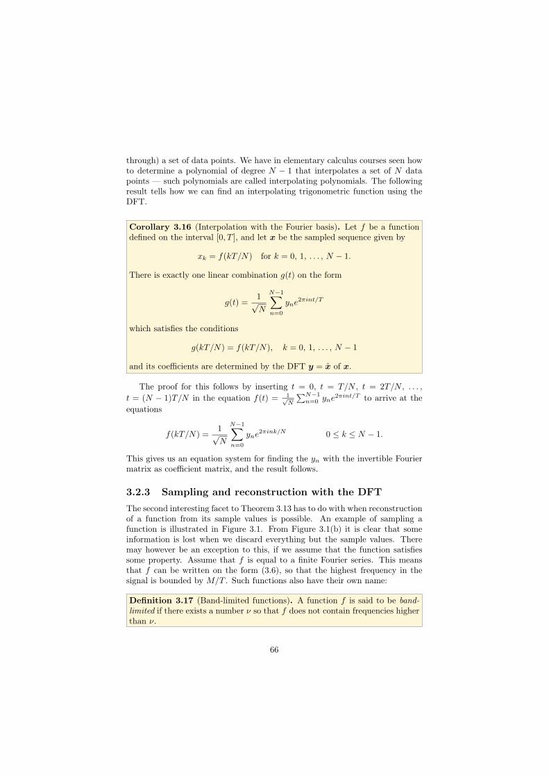
Figure 3.1: An example of sampling. Figure (a) shows how the samples arepicked from underlying continuous time function. Figure (b) shows what thesamples look like on their own.
0.2 0.4 0.6 0.8 1.0
�1.0
�0.5
0.5
1.0
(a)
0.2 0.4 0.6 0.8 1.0
�1.0
�0.5
0.5
1.0
(b)
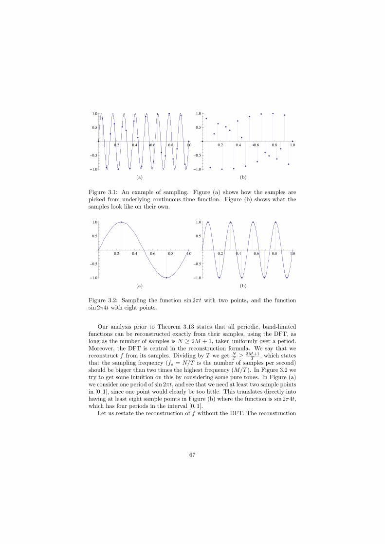
Figure 3.2: Sampling the function sin 2πt with two points, and the functionsin 2π4t with eight points.
Our analysis prior to Theorem 3.13 states that all periodic, band-limitedfunctions can be reconstructed exactly from their samples, using the DFT, aslong as the number of samples is N ≥ 2M + 1, taken uniformly over a period.Moreover, the DFT is central in the reconstruction formula. We say that wereconstruct f from its samples. Dividing by T we get N
T≥ 2M+1
T, which states
that the sampling frequency (fs = N/T is the number of samples per second)should be bigger than two times the highest frequency (M/T ). In Figure 3.2 wetry to get some intuition on this by considering some pure tones. In Figure (a)we consider one period of sin 2πt, and see that we need at least two sample pointsin [0, 1], since one point would clearly be too little. This translates directly intohaving at least eight sample points in Figure (b) where the function is sin 2π4t,which has four periods in the interval [0, 1].
Let us restate the reconstruction of f without the DFT. The reconstruction
67

formula was
f(t) =1√N
M�
n=−M
yne2πint/T .
If we here substitute y = FNx we get that this equals
1
N
M�
n=−M
N−1�
k=0
xke−2πink/Ne2πint/T
=N−1�
k=0
1
N
�M�
n=−M
xke2πin(t/T−k/N)
�
=N−1�
k=0
1
Ne−2πiM(t/T−k/N) 1− e2πi(2M+1)(t/T−k/N)
1− e2πi(t/T−k/N)xk
=N−1�
k=0
1
N
sin(π(t− kTs)/Ts)
sin(π(t− kTs)/T )f(kTs),
where we have substituted N = T/Ts (deduced from T = NTs with Ts beingthe sampling period). Let us summarize our findings as follows:
Theorem 3.18 (Sampling theorem and the ideal interpolation formula forperiodic functions). Let f be a periodic function with period T , and assumethat f has no frequencies higher than νHz. Then f can be reconstructedexactly from its samples f(0), . . . , f((N − 1)Ts) (where Ts is the samplingperiod and N = T
Tsis the number of samples per period) when the sampling
rate Fs =1Ts
is bigger than 2ν. Moreover, the reconstruction can be performedthrough the formula
f(t) =N−1�
k=0
f(kTs)1
N
sin(π(t− kTs)/Ts)
sin(π(t− kTs)/T ). (3.10)
Formula (3.10) is also called the ideal interpolation formula for periodicfunctions. Such formulas, where one reconstructs a function based on a weightedsum of the sample values, are more generally called interpolation formulas. Wewill return to other interpolation formulas later, which have different properties.
Note that f itself may not be equal to a finite Fourier series, and reconstruc-tion is in general not possible then. Interpolation as performed in Section 3.2.2is still possible, however, but the g(t) we obtain from Corollary 3.16 may bedifferent from f(t).
Exercises for Section 3.2
Ex. 1 — Compute the 4 point DFT of the vector (2, 3, 4, 5)T .
68

Ex. 2 — As in Example 3.9, state the exact cartesian form of the Fouriermatrix for the cases N = 6, N = 8, and N = 12.
Ex. 3 — Let x be the vector with entries xk = ck. Show that the DFT of xis given by the vector with components
yn =1√N
1− cN
1− ce−2πin/N
for n = 0, . . . , N − 1.
Ex. 4 — If x is complex, Write the DFT in terms of the DFT on real se-quences. Hint: Split into real and imaginary parts, and use linearity of theDFT.
Ex. 5 — As in Example 3.10, write a function
function x=IDFTImpl(y)
which computes the IDFT.
Ex. 6 — Let G be the N × (2M + 1)-matrix with entries 1√Ne2πink/N , and
H the N ×N -matrix with entries 1√Ne2πink/N . Show that GHG = I2M+1 and
that GHH =�I 0
�when N ≥ 2M + 1. Write also down an expression for
GHG when N < 2M +1, to show that it is in general different from the identitymatrix.
3.3 Operations on vectors: filters
In Chapter 1 we defined some operations on digital sounds, which we looselyreferred to as filters. One example was the averaging filter
zn =1
4(xn−1 + 2xn + xn+1), for n = 0, 1, . . . , N − 1 (3.11)
of Example 1.25 where x denotes the input vector and z the output vector.Before we state the formal definition of filters, let us consider Equation (3.11)in some more detail to get more intuition about filters.
As before we assume that the input vector is periodic with period N , so thatxn+N = xn. Our first observation is that the output vector z is also periodicwith period N since
zn+N =1
4(xn+N−1 + 2xn+N + xn+N+1) =
1
4(xn−1 + 2xn + xn+1) = zn.
69

The filter is also clearly a linear transformation and may therefore be representedby an N × N matrix S that maps the vector x = (x0, x1, . . . , xN−1) to thevector z = (z0, z1, . . . , zN−1), i.e., we have z = Sx. To find S we note that for1 ≤ n ≤ N − 2 it is clear from Equation (3.11) that row n has the value 1/4 incolumn n − 1, the value 1/2 in column n, and the value 1/4 in column n + 1.For row 0 we must be a bit more careful, since the index −1 is outside the legalrange of the indices. This is where the periodicity helps us out so that
z0 =1
4(x−1 + 2x0 + x1) =
1
4(xN−1 + 2x0 + x1) =
1
4(2x0 + x1 + xN−1).
From this we see that row 0 has the value 1/4 in columns 1 and N − 1, and thevalue 1/2 in column 0. In exactly the same way we can show that row N − 1has the entry 1/4 in columns 0 and N − 2, and the entry 1/2 in column N − 1.In summary, the matrix of the averaging filter is given by
S =1
4
2 1 0 0 · · · 0 0 0 11 2 1 0 · · · 0 0 0 00 1 2 1 · · · 0 0 0 0...
......
......
......
......
0 0 0 0 · · · 0 1 2 11 0 0 0 · · · 0 0 1 2
. (3.12)
A matrix on this form is called a Toeplitz matrix. Such matrices are verypopular in the literature and have many applications. The general definitionmay seem complicated, but is in fact quite straightforward:
Definition 3.19 (Toeplitz matrices). An N ×N -matrix S is called a Toeplitzmatrix if its elements are constant along each diagonal. More formally, Sk,l =Sk+s,l+s for all nonnegative integers k, l, and s such that both k+ s and l+ slie in the interval [0, N − 1]. A Toeplitz matrix is said to be circulant if inaddition
S(k+s) mod N,(l+s) mod N = Sk,l
for all integers k, l in the interval [0, N − 1], and all s (Here mod denotes theremainder modulo N).
As the definition says, a Toeplitz matrix is constant along each diagonal,while the additional property of being circulant means that each row and columnof the matrix ’wraps over’ at the edges. It is quite easy to check that the matrixS given by Equation (3.12) satisfies Definition 3.19 and is a circulant Toeplitzmatrix. A Toeplitz matrix is uniquely identified by the values on its nonzerodiagonals, and a circulant Toeplitz matrix is uniquely identified by the N/2diagonals above or on the main diagonal, and the N/2 diagonals below themain diagonal. We will encounter Toeplitz matrices also in other contexts inthese notes.
70
In Chapter 1, the operations we loosely referred to as filters, such as for-mula (3.11), could all be written on the form
zn =�
k
tkxn−k. (3.13)
Many other operations are also defined in this way. The values tk will be calledfilter coefficients. The range of k is not specified, but is typically an intervalaround 0, since zn usually is calculated by combining xks with indices closeto n. Both positive and negative indices are allowed. As an example, for for-mula (3.11) k ranges over −1, 0, and 1, and we have that t−1 = t1 = 1/4, andt0 = 1/2. By following the same argument as above, the following is clear:
Proposition 3.20. Any operation defined by Equation (3.13) is a linear trans-formation which transforms a vector of period N to another of period N . Itmay therefore be represented by an N × N matrix S that maps the vectorx = (x0, x1, . . . , xN−1) to the vector z = (z0, z1, . . . , zN−1), i.e., we havez = Sx. Moreover, the matrix S is a circulant Toeplitz matrix, and the firstcolumn s of this matrix is given by
sk =
�tk, if 0 ≤ k < N/2;
tk−N if N/2 ≤ k ≤ N − 1.(3.14)
In other words, the first column of S can be obtained by placing the coefficientsin (3.13) with positive indices at the beginning of s, and the coefficients withnegative indices at the end of s.
This proposition will be useful for us, since it explains how to pass from theform (3.13), which is most common in practice, to the matrix form S.
Example 3.21. Let us apply Proposition 3.20 on the operation defined byformula (3.11):
1. for k = 0 Equation 3.14 gives s0 = t0 = 1/2.
2. For k = 1 Equation 3.14 gives s1 = t1 = 1/4.
3. For k = N − 1 Equation 3.14 gives sN−1 = t−1 = 1/4.
For all k different from 0, 1, and N − 1, we have that sk = 0. Clearly this givesthe matrix in Equation (3.12).
Proposition 3.20 is also useful when we have a circulant Toeplitz matrix S,and we want to find filter coefficients tk so that z = Sx can be written as inEquation (3.13):
71
Example 3.22. Consider the matrix
S =
2 1 0 33 2 1 00 3 2 11 0 3 2
.
This is a circulant Toeplitz matrix with N = 4, and we see that s0 = 2, s1 = 3,s2 = 0, and s3 = 1. The first equation in (3.14) gives that t0 = s0 = 2, andt1 = s1 == 3. The second equation in (3.14) gives that t−2 = s2 = 0, andt−1 = s3 = 1. By including only the tk which are nonzero, the operation can bewritten as
zn = t−1xn−(−1) + t0xn + t1xn−1 + t2xn−2 = xn+1 + 2x0 + 3xn−1.
3.3.1 Formal definition of filters and frequency response
Let us now define filters formally, and establish their relationship to Toeplitzmatrices. We have seen that a sound can be decomposed into different frequencycomponents, and we would like to define filters as operations which adjust thesefrequency components in a predictable way. One such example is provided inExample 3.15, where we simply set some of the frequency components to 0. Thenatural starting point is to require for a filter that the output of a pure tone isa pure tone with the same frequency.
Definition 3.23 (Digital filters and frequency response). A linear transfor-mation S : RN �→ RN is a said to be a digital filter, or simply a filter, if itmaps any Fourier vector in RN to a multiple of itself. In other words, for anyinteger n in the range 0 ≤ n ≤ N − 1 there exists a value λS,n so that
S (φn) = λS,nφn, (3.15)
i.e., the N Fourier vectors are the eigenvectors of S. The vector of (eigen)valuesλS = (λS,n)
N−1n=0 is often referred to as the frequency response of S.
We will identify the linear transformation S with its matrix relative to thestandard basis. Since the Fourier basis vectors are orthogonal vectors, S isclearly orthogonally diagonalizable. Since also the Fourier basis vectors are thecolumns in (FN )H , we have that
S = FH
NDFN (3.16)
whenever S is a digital filter, where D has the frequency response (i.e. theeigenvalues) on the diagonal1. In particular, if S1 and S2 are digital filters, we
1Recall that the orthogonal diagonalization of S takes the form S = PDPT , where Pcontains as columns an orthonormal set of eigenvectors, and D is diagonal with the eigenvectorslisted on the diagonal (see Section 7.1 in [7]).
72
can write S1 = FH
ND1FN and S2 = FH
ND2FN , so that
S1S2 = FH
ND1FNFH
ND2FN = FH
ND1D2FN .
Since D1D2 = D2D1 for any diagonal matrices, we get the following corollary:
Corollary 3.24. All digital filters commute, i.e. if S1 and S2 are digitalfilters, S1S2 = S2S1.
There are several equivalent characterizations of a digital filter. The first onewas stated above in terms of the definition through eigenvectors and eigenvalues.The next characterization helps us prove that the operations from Chapter 1actually are filters.
Theorem 3.25. A linear transformation S is a digital filter if and only if itis a circulant Toeplitz matrix.
Proof. That S is a filter is equivalent to the fact that S = (FN )HDFN for somediagonal matrix D. We observe that the entry at position (k, l) in S is given by
Sk,l =1
N
N−1�
n=0
e2πikn/NλS,ne−2πinl/N =
1
N
N−1�
n=0
e2π(k−l)n/NλS,n.
Another entry on the same diagonal (shifted s rows and s columns) is
S(k+s) mod N,(l+s) mod N =1
N
N−1�
n=0
e2πi((k+s) mod N−(l+s) mod N)n/NλS,n
=1
N
N−1�
n=0
e2πi(k−l)n/NλS,n = Sk,l,
which proves that S is a circulant Toeplitz matrix.
In particular, operations defined by (3.13) are digital filters, when restrictedto vectors with period N . The following results enables us to compute theeigenvalues/frequency response easily, so that we do not need to form the char-acteristic polynomial and find its roots:
Theorem 3.26. Any digital filter is uniquely characterized by the values inthe first column of its matrix. Moreover, if s is the first column in S, thefrequency response of S is given by
λS =√NFNs. (3.17)
Conversely, if we know the frequency response λS , the first column s of S isgiven by
s =1√N
(FN )HλS . (3.18)
73
Proof. If we replace S by (FN )HDFN we find that
FNs = FNS
10...0
= FNFH
NDFN
10...0
= DFN
10...0
=
1√N
D
1...1
,
where we have used the fact that the first column in FN has all entries equalto 1/
√N . But the the diagonal matrix D has all the eigenvalues of S on its
diagonal, and hence the last expression is the vector of eigenvalues λS , whichproves (3.17). Equation (3.18) follows directly by applying the inverse DFT to(3.17).
Since the first column s characterizes the filter S uniquely, one often refersto S by the vector s. The first column s is also called the impulse response.This name stems from the fact that we can write s = Se0, i.e., the vector s isthe output (often called response) to the vector e0 (often called an impulse).
Example 3.27. The identity matrix is a digital filter since I = (FN )HIFN .Since e0 = Se0, it has impulse response s = e0. Its frequency response has 1 inall components and therefore preserves all frequencies, as expected.
Equations (3.16), (3.17), and (3.18) are important relations between thematrix- and frequency representations of a filter. We see that the DFT is acrucial ingredient in these relations. A consequence is that, once you recognizea matrix as circulant Toeplitz, you do not need to make the tedious calculationof eigenvectors and eigenvalues which you are used to. Let us illustrate thiswith an example.
Example 3.28. Let us compute the eigenvalues and eigenvectors of the simplematrix
S =
�4 11 4
�.
It is straightforward to compute the eigenvalues and eigenvectors of this matrixthe way you learnt in your first course in linear algebra. However, this matrixis also a circulant Toeplitz matrix, so that we can also use the results in thissection to compute the eigenvalues and eigenvectors. Since here N = 2, we havethat e2πink/N = eπink = (−1)nk. This means that the Fourier basis vectors are(1, 1)/
√2 and (1,−1)/
√2, which also are the eigenvectors of S. The eigenvalues
are the frequency response of S, which can be obtained as
√NFNs =
√2
1√2
�1 11 −1
��41
�=
�53
�
The eigenvalues are thus 3 and 5. You could have obtained the same resultwith Matlab. Note that Matlab may not return the eigenvectors exactly as theFourier basis vectors, since the eigenvectors are not unique (the multiple of an
74

eigenvector is still an eigenvector). In this case Matlab may for instance switchthe signs of the eigenvectors. We have no control over what Matlab actuallychooses to do, since it uses some underlying numerical algorithm for computingeigenvectors which we can’t influence.
In signal processing, the frequency content of a vector (i.e., its DFT) isalso referred to as its spectrum. This may be somewhat confusing from a linearalgebra perspective, because in this context the term spectrum is used to denotethe eigenvalues of a matrix. But because of Theorem 3.26 this is not so confusingafter all if we interpret the spectrum of a vector (in signal processing terms) asthe spectrum of the corresponding digital filter (in linear algebra terms).
3.3.2 Some properties of the frequency response
Equation (3.17) states that the frequency response can be written as
λS,n =N−1�
k=0
ske−2πink/N , for n = 0, 1, . . . , N − 1, (3.19)
where sk are the components of the impulse response s.
Example 3.29. When only few of the coefficients sk are nonzero, it is possibleto obtain nice expressions for the frequency response. To see this, let us computethe frequency response of the filter defined from formula (3.11). We saw thatthe first column of the corresponding Toeplitz matrix satisfied s0 = 1/2, andsN−1 = s1 = 1/4. The frequency response is thus
λS,n =1
2e0 +
1
4e−2πin/N +
1
4e−2πin(N−1)/N
=1
2e0 +
1
4e−2πin/N +
1
4e2πin/N =
1
2+
1
2cos(2πn/N).
If we make the substitution ω = 2πn/N in the formula for λS,n, we may in-terpret the frequency response as the values on a continuous function on [0, 2π).
Theorem 3.30. The function λS(ω) defined on [0, 2π) by
λS(ω) =�
k
tke−ikω, (3.20)
where tk are the filter coefficients of S, satisfies
λS,n = λS(2πn/N) for n = 0, 1, . . . , N − 1
for any N . In other words, regardless of N , the frequency reponse lies on thecurve λS .
75

Proof. For any N we have that
λS,n =N−1�
k=0
ske−2πink/N =
�
0≤k<N/2
ske−2πink/N +
�
N/2≤k≤N−1
ske−2πink/N
=�
0≤k<N/2
tke−2πink/N +
�
N/2≤k≤N−1
tk−Ne−2πink/N
=�
0≤k<N/2
tke−2πink/N +
�
−N/2≤k≤−1
tke−2πin(k+N)/N
=�
0≤k<N/2
tke−2πink/N +
�
−N/2≤k≤−1
tke−2πink/N
=�
−N/2≤k<N/2
tke−2πink/N = λS(ω).
where we have used Equation (3.14).
Both λS(ω) and λS,n will be referred to as frequency responses in the fol-lowing. When there is a need to distinguish the two we will call λS,n the vectorfrequency response, and λS(ω)) the continuous frequency response. ω is alsocalled angular frequency.
The difference in the definition of the continuous- and the vector frequencyresponse lies in that one uses the filter coefficients tk, while the other uses theimpulse response sk. While these contain the same values, they are stored dif-ferently. Had we used the impulse response to define the continuous frequencyresponse, we would have needed to compute
�N−1k=0 ske−πiω, which does not con-
verge when N → ∞ (although it gives the right values at all points ω = 2πn/Nfor all N)! The filter coefficcients avoid this convergence problem, however,since we assume that only tk with |k| small are nonzero. In other words, filtercoefficients are used in the definition of the continuous frequency response sothat we can find a continuous curve where we can find the vector frequencyresponse values for all N .
The frequency response contains the important characteristics of a filter,since it says how it behaves for the different frequencies. When analyzing afilter, we therefore often plot the frequency response. Often we plot only theabsolute value (or the magnitude) of the frequency response, since this is whatexplains how each frequency is amplified or attenuated. Since λS is clearlyperiodic with period 2π, we may restrict angular frequency to the interval [0, 2π).The conclusion in Observation 3.14 was that the low frequencies in a vectorcorrespond to DFT indices close to 0 and N−1, and high frequencies correspondto DFT indices close to N/2. This observation is easily translated to a statementabout angular frequencies:
Observation 3.31. When plotting the frequency response on [0, 2π), angularfrequencies near 0 and 2π correspond to low frequencies, angular frequenciesnear π correspond to high frequencies
76
1 2 3 4 5 6
0.2
0.4
0.6
0.8
1.0
(a)
�3 �2 �1 1 2 3
0.2
0.4
0.6
0.8
1.0
(b)
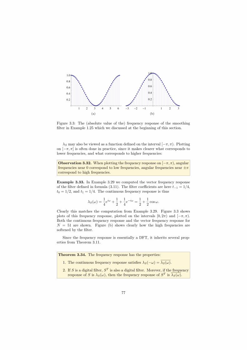
Figure 3.3: The (absolute value of the) frequency response of the smoothingfilter in Example 1.25 which we discussed at the beginning of this section.
λS may also be viewed as a function defined on the interval [−π,π). Plottingon [−π,π] is often done in practice, since it makes clearer what corresponds tolower frequencies, and what corresponds to higher frequencies:
Observation 3.32. When plotting the frequency response on [−π,π), angularfrequencies near 0 correspond to low frequencies, angular frequencies near ±πcorrespond to high frequencies.
Example 3.33. In Example 3.29 we computed the vector frequency responseof the filter defined in formula (3.11). The filter coefficients are here t−1 = 1/4,t0 = 1/2, and t1 = 1/4. The continuous frequency response is thus
λS(ω) =1
4eiω +
1
2+
1
4e−iω =
1
2+
1
2cosω.
Clearly this matches the computation from Example 3.29. Figure 3.3 showsplots of this frequency response, plotted on the intervals [0, 2π) and [−π,π).Both the continuous frequency response and the vector frequency response forN = 51 are shown. Figure (b) shows clearly how the high frequencies aresoftened by the filter.
Since the frequency response is essentially a DFT, it inherits several prop-erties from Theorem 3.11.
Theorem 3.34. The frequency response has the properties:
1. The continuous frequency response satisfies λS(−ω) = λS(ω).
2. If S is a digital filter, ST is also a digital filter. Morever, if the frequencyresponse of S is λS(ω), then the frequency response of ST is λS(ω).
77

3. If S is symmetric, λS is real. Also, if S is antisymmetric (the element onthe opposite side of the diagonal is the same, but with opposite sign),λS is purely imaginary.
4. If S1 and S2 are digital filters, then S1S2 also is a digital filter, andλS1S2(ω) = λS1(ω)λS2(ω).
Proof. Property 1. and 3. follow directly from Theorem 3.11. Transposing amatrix corresponds to reversing the first colum of the matrix and thus also thefilter coefficients. Due to this Property 2. also follows from Theorem 3.11. Thelast property follows in the same was as we showed that filters commute:
S1S2 = (FN )HD1FN (FN )HD2FN = (FN )HD1D2FN .
The frequency response of S1S2 is thus obtained by multiplying the frequencyresponses of S1 and S2.
In particular the frequency response may not be real, although this wasthe case in the first example of this section. Theorem 3.34 applies both forthe vector- and continuous frequency response. Also, clearly S1 + S2 is a filterwhen S1 and S2 are. The set of all filters is thus a vector space, which also isclosed under multiplication. Such a space is called an algebra. Since all filterscommute, this algebra is also called a commutative algebra.
Example 3.35. Assume that the filters S1 and S2 have the frequency responsesλS1(ω) = cos(2ω), λS2(ω) = 1+3 cosω. Let us see how we can use Theorem 3.34to compute the filter coefficients and the matrix of the filter S = S1S2. We firstnotice that, since both frequency responses are real, all S1, S2, and S = S1S2
are symmetric. We rewrite the frequency responses as
λS1(ω) =1
2(e2iω + e−2iω) =
1
2e2iω +
1
2e−2iω
λS2(ω) = 1 +3
2(eiω + e−iω) =
3
2eiω + 1 +
3
2e−iω.
We now get that
λS1S2(ω) = λS1(ω)λS2(ω) =
�1
2e2iω +
1
2e−2iω
��3
2eiω + 1 +
3
2e−iω
�
=3
4e3iω +
1
2e2iω +
3
4eiω +
3
4e−iω +
1
2e−2iω +
3
4e−3iω
From this expression we see that the filter coefficients of S are t±1 = 3/4,t±2 = 1/2, t±3 = 3/4. All other filter coefficients are 0. Using Theorem 3.20,we get that s1 = 3/4, s2 = 1/2, and s3 = 3/4, while sN−1 = 3/4, sN−2 = 1/2,and sN−3 = 3/4 (all other sk are 0). This gives us the matrix representation ofS.
78

3.3.3 Assembling the filter matrix and compact notation
Let us return to how we first defined a filter in Equation (3.13):
zn =�
k
tkxn−k.
As mentioned, the range of k may not be specified. In some applications insignal processing there may in fact be infinitely many nonzero tk. However,when x is assumed to have period N , we may as well assume that the k’s rangeover an interval of length N (else many of the tk’s can be added together tosimplify the formula). Also, any such interval can be chosen. It is common tochoose the interval so that it is centered around 0 as much as possible. For this,we can choose for instance [�N/2� − N + 1, �N/2�]. With this choice we canwrite Equation (3.13) as
zn =
�N/2��
k=�N/2�−N+1
tkxn−k. (3.21)
The index range in this sum is typically even smaller, since often much less thanN of the tk are nonzero (For Equation (3.11), there were only three nonzero tk).In such cases one often uses a more compact notation for the filter:
Definition 3.36 (Compact notation for filters). Let kmin ≤ 0, kmax ≥ 0 bethe smallest and biggest index of a filter coefficient in Equation (3.21) so thattk �= 0 (if no such values exist, let kmin = 0, or kmax = 0), i.e.
zn =kmax�
k=kmin
tkxn−k. (3.22)
We will use the following compact notation for S:
S = {tkmin , . . . , t−1, t0, t1, . . . , tkmax}.
In other words, the entry with index 0 has been underlined, and only thenonzero tk’s are listed. By the length of S, denoted l(S), we mean the numberkmax − kmin.
One seldom writes out the matrix of a filter, but rather uses this compactnotation. Note that the length of S can also be written as the number of nonzerofilter coefficients minus 1. l(S) thus follows the same convention as the degreeof a polynomial: It is 0 if the polynomial is constant (i.e. one nonzero filtercoefficient).
Example 3.37. Using the compact notation for a filter, we would write S ={1/4, 1/2, 1/4} for the filter given by formula (3.11)). For the filter
zn = xn+1 + 2x0 + 3xn−1
79

from Example 3.22, we would write S = {1, 2, 3}.
Equation (3.13) is also called the convolution of the two vectors t and x.Convolution is usually defined without the assumption that the vectors are pe-riodic, and without any assumption on their lengths (i.e. they may be sequencesof inifinite length):
Definition 3.38 (Convolution of vectors). By the convolution of two vectorsx and y we mean the vector x ∗ y defined by
(x ∗ y)n =�
k
xkyn−k. (3.23)
In other words, applying a filter S corresponds to convolving the filter co-efficients of S with the input. If both x and y have infinitely many nonzeroentries, the sum is an infinite one, which may diverge. For the filters we lookat, we always have a finite number of nonzero entries tk, so we never have thisconvergence problem since the sum is a finite one. MATLAB has the built-infunction conv for convolving two vectors of finite length. This function does notindicate which indices the elements of the returned vector belongs to, however.Exercise 11 explains how one may keep track of these indices.
Since the number of nonzero filter coefficients is typically much less than N(the period of the input vector), the matrix S have many entries which are zero.Multiplication with such matrices requires less additions and multiplicationsthan for other matrices: If S has k nonzero filter coefficients, S has Nk nonzeroentries, so that kN multiplications and (k−1)N additions are needed to computeSx. This is much less than the N2 multiplications and (N − 1)N additionsneeded in the general case. Perhaps more important is that we need not formthe entire matrix, we can perform the matrix multiplication directly in a loop.Exercise 10 investigates this further. For large N we risk running into out ofmemory situations if we had to form the entire matrix.
3.3.4 Some examples of filters
We have now established the basic theory of filters, so it is time to study somespecific examples. Many of the filters below were introduced in Section 1.4.
Example 3.39 (Time delay filters). The simplest possible type of Toeplitzmatrix is one where there is only one nonzero diagonal. Let us define the Toeplitzmatrix Ed as the one which has first column equal to ed. In the notation above,and when d > 0, this filter can also be written as S = {0, . . . , 1} where the 1occurs at position d. We observe that
(Edx)n =N−1�
k=0
(Ed)n,k xk =N−1�
k=0
(Ed)(n−k) mod N,0 xk = x(n−d) mod N ,
80
0 2 4 60
0.2
0.4
0.6
0.8
1
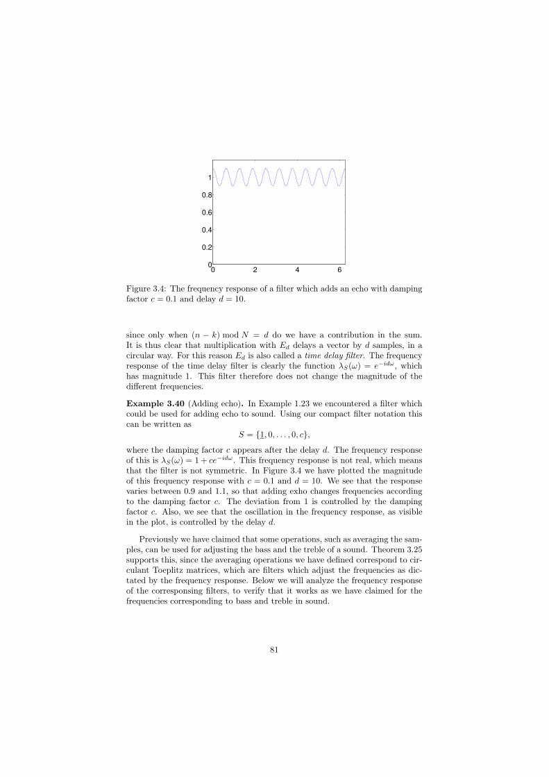
Figure 3.4: The frequency response of a filter which adds an echo with dampingfactor c = 0.1 and delay d = 10.
since only when (n − k) mod N = d do we have a contribution in the sum.It is thus clear that multiplication with Ed delays a vector by d samples, in acircular way. For this reason Ed is also called a time delay filter. The frequencyresponse of the time delay filter is clearly the function λS(ω) = e−idω, whichhas magnitude 1. This filter therefore does not change the magnitude of thedifferent frequencies.
Example 3.40 (Adding echo). In Example 1.23 we encountered a filter whichcould be used for adding echo to sound. Using our compact filter notation thiscan be written as
S = {1, 0, . . . , 0, c},
where the damping factor c appears after the delay d. The frequency responseof this is λS(ω) = 1+ ce−idω. This frequency response is not real, which meansthat the filter is not symmetric. In Figure 3.4 we have plotted the magnitudeof this frequency response with c = 0.1 and d = 10. We see that the responsevaries between 0.9 and 1.1, so that adding exho changes frequencies accordingto the damping factor c. The deviation from 1 is controlled by the dampingfactor c. Also, we see that the oscillation in the frequency response, as visiblein the plot, is controlled by the delay d.
Previously we have claimed that some operations, such as averaging the sam-ples, can be used for adjusting the bass and the treble of a sound. Theorem 3.25supports this, since the averaging operations we have defined correspond to cir-culant Toeplitz matrices, which are filters which adjust the frequencies as dic-tated by the frequency response. Below we will analyze the frequency responseof the corresponsing filters, to verify that it works as we have claimed for thefrequencies corresponding to bass and treble in sound.
81

Example 3.41 (Reducing the treble). In Example 1.25 we encountered themoving average filter
S =
�1
3,1
3,1
3
�.
This could be used for reducing the treble in a sound. If we set N = 4, thecorresponding circulant Toeplitz matrix for the filter is
S =1
3
1 1 0 11 1 1 00 1 1 11 0 1 1
The frequency response is λS(ω) = (eiω +1+ e−iω)/3 = (1+ 2 cos(ω))/3. Moregenerally, if the filter is s = (1, · · · , 1, · · · , 1)/(2L+1), where there is symmetryaround 0, we recognize this as x/(2L+1), where x is a vector of ones and zeros,as defined in Example 3.8. From that example we recall that
x =1√N
sin(πn(2L+ 1)/N)
sin(πn/N),
so that the frequency response of S is
λS,n =1
2L+ 1
sin(πn(2L+ 1)/N)
sin(πn/N),
andλS(ω) =
1
2L+ 1
sin((2L+ 1)ω/2)
sin(ω/2).
We clearly have
0 ≤ 1
2L+ 1
sin((2L+ 1)ω/2)
sin(ω/2)≤ 1,
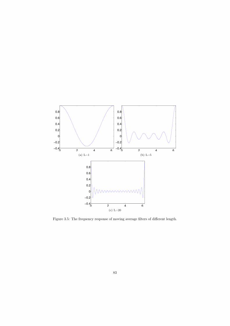
so this frequency response approaches 1 as ω → 0+. The frequency responsethus peaks at 0, and it is clear that this peak gets narrower and narrower asL increases, i.e. we use more and more samples in the averaging process. Thisappeals to our intuition that this kind of filters smooths the sound by keepingonly lower frequencies. In Figure 3.5 we have plotted the frequency response formoving average filters with L = 1, L = 5, and L = 20. We see, unfortunately,that the frequency response is far from a filter which keeps some frequenciesunaltered, while annihilating others (this is a desirable property which is referedto as being a bandpass filter): Although the filter distinguishes between high andlow frequencies, it slightly changes the small frequencies. Moreover, the higherfrequencies are not annihilated, even when we increase L to high values.
In the previous example we mentioned a filter which kept some frequenciesunaltered, and annihilated others. This is a desirable property for filters, so letus give names to such filters:
82
0 2 4 6!0.4
!0.2
0
0.2
0.4
0.6
0.8
(a) L=10 2 4 6
!0.4
!0.2
0
0.2
0.4
0.6
0.8
(b) L=5
0 2 4 6!0.4
!0.2
0
0.2
0.4
0.6
0.8
(c) L=20
Figure 3.5: The frequency response of moving average filters of different length.
83

Definition 3.42. A filter S is called
1. a lowpass filter if λS(ω) ≈ 1 when ω is close to 0, and λS(ω) ≈ 0 when ω isclose to π (i.e. S keeps low frequencies and annhilates high frequencies),
2. a highpass filter if λS(ω) ≈ 1 when ω is close to π, and λS(ω) ≈ 0when ω is close to 0 (i.e. S keeps high frequencies and annhilates lowfrequencies),
3. a bandpass filter if λS(ω) ≈ 1 within some interval [a, b] ⊂ [0, 2π], andλS(ω) ≈ 0 outside this interval.
This definition should be considered rather vague when it comes to what wemean by “ω close to 0,π”, and “λS(ω) ≈ 0, 1”: in practice, when we talk aboutlowpass and highpass filters, it may be that the frequency responses are stillquite far from what is commonly refered to as ideal lowpass or highpass filters,where the frequency response only assumes the values 0 and 1 near 0 and π.The next example considers an ideal lowpass filter.
Example 3.43 (Ideal lowpass filters). By definition, the ideal lowpass filterkeeps frequencies near 0, and removes frequencies near π. In Chapter 1 wementioned that we were not able to find the filter coefficients for such a filter.We now have the theory in place in order to achieve this: In Example 3.15 weimplemented the ideal lowpass filter with the help of the DFT. Mathematically,the code was equivalent to computing (FN )HDFN where D is the diagonalmatrix with the entries 0, . . . , L and N − L, . . . , N − 1 being 1, the rest being0. Clearly this is a digital filter, with frequency response as stated. If thefilter should keep the angular frequencies |ω| ≤ ωc only, where ωc describes thehighest frequency we should keep, we should choose L so that ωc = 2πL/N .In Example 3.8 we computed the DFT of this vector, and it followed fromTheorem 3.11 that the IDFT of this vector equals its DFT. This means thatwe can find the filter coefficients by using Equation (3.18): Since the IDFT was1√N
sin(πk(2L+1)/N)sin(πk/N) , the filter coefficients are
1√N
1√N
sin(πk(2L+ 1)/N)
sin(πk/N)=
1
N
sin(πk(2L+ 1)/N)
sin(πk/N).
This means that the filter coefficients lie as N points uniformly spaced on thecurve 1
N
sin(ω(2L+1)/2)sin(ω/2) between 0 and π. This curve has been encountered many
other places in these notes. The filter which keeps only the frequency ωc = 0 hasall filter coefficients being 1
N(set L = 1), and when we include all frequencies
(set L = N) we get the filter where x0 = 1 and all other filter coefficientsare 0. When we are between these two cases, we get a filter where s0 is thebiggest coefficient, while the others decrease towards 0 along the curve we havecomputed. The bigger L and N are, the quicker they decrease to zero. Allfilter coefficients are typically nonzero for this filter, since this curve is zero
84
only at certain points. This is unfortunate, since it means that the filter istime-consuming to compute.
The two previous examples show an important duality between vectors whichare 1 on some elements and 0 on others (also called window vectors), and thevector 1
N
sin(πk(2L+1)/N)sin(πk/N) (also called a sinc): filters of the one type correspond
to frequency responses of the other type, and vice versa. The examples alsoshow that, in some cases only the filter coefficients are known, while in othercases only the frequency response is known. In any case we can deduce the onefrom the other, and both cases are important.
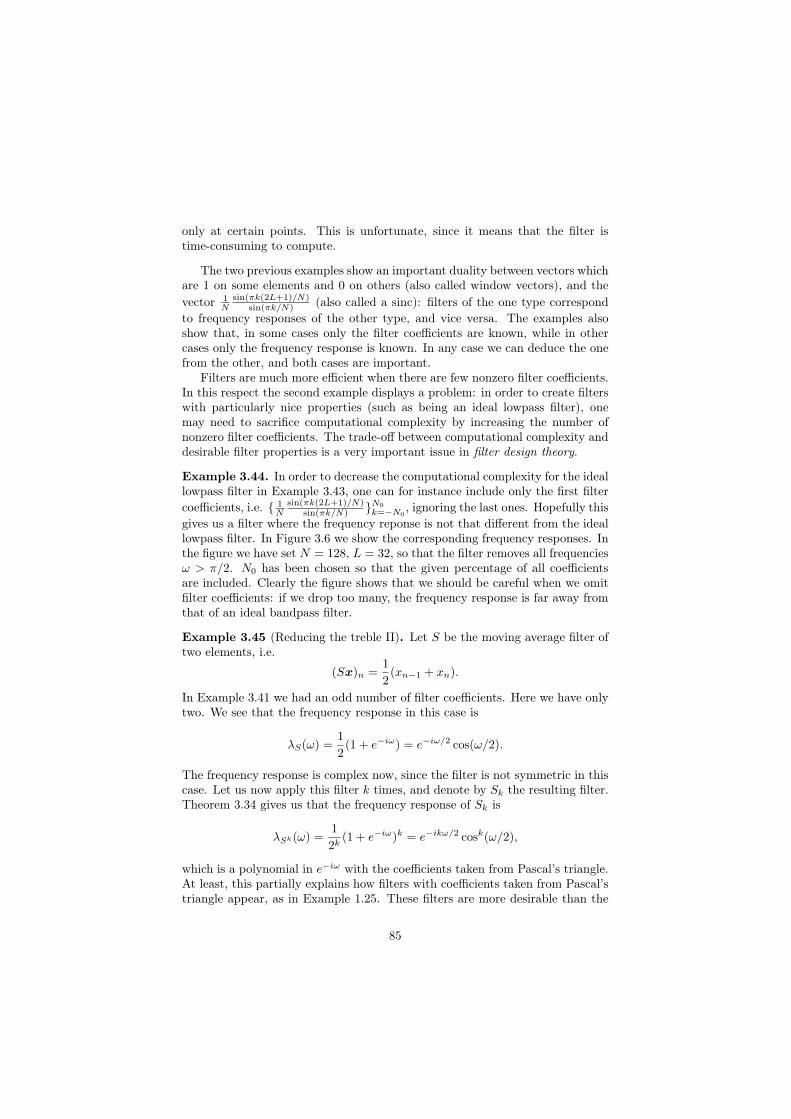
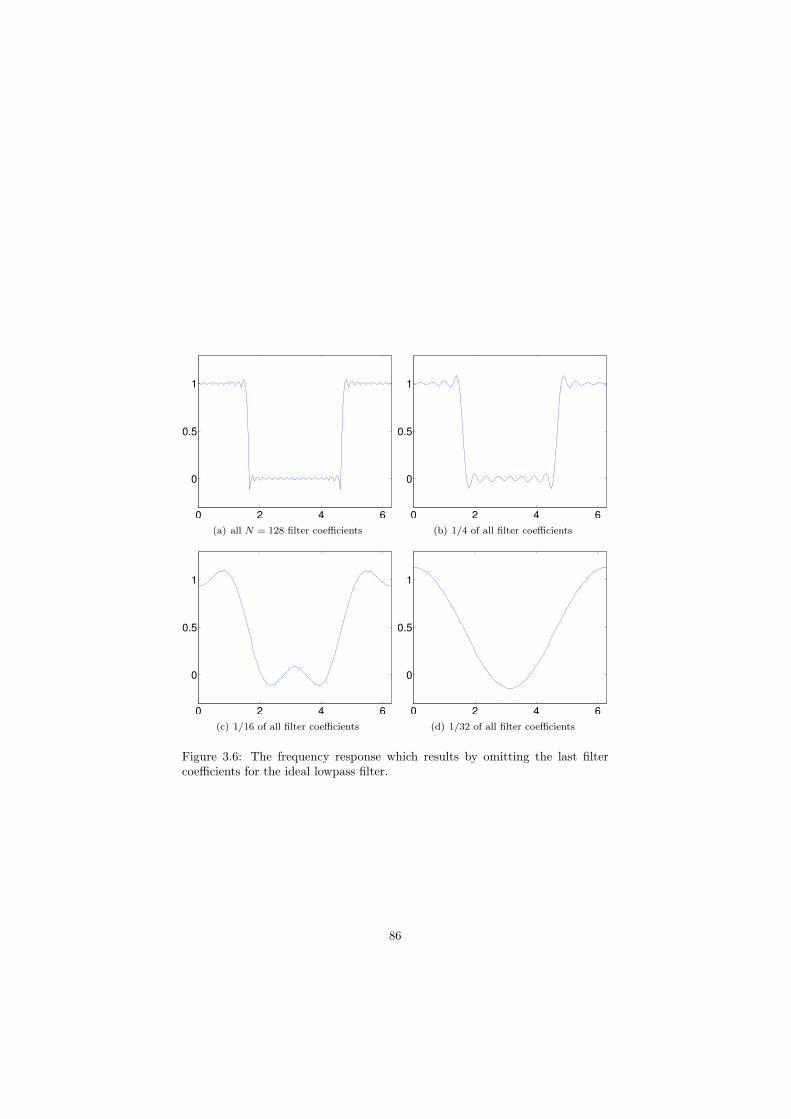
Filters are much more efficient when there are few nonzero filter coefficients.In this respect the second example displays a problem: in order to create filterswith particularly nice properties (such as being an ideal lowpass filter), onemay need to sacrifice computational complexity by increasing the number ofnonzero filter coefficients. The trade-off between computational complexity anddesirable filter properties is a very important issue in filter design theory.
Example 3.44. In order to decrease the computational complexity for the ideallowpass filter in Example 3.43, one can for instance include only the first filtercoefficients, i.e. { 1
N
sin(πk(2L+1)/N)sin(πk/N) }N0
k=−N0, ignoring the last ones. Hopefully this
gives us a filter where the frequency reponse is not that different from the ideallowpass filter. In Figure 3.6 we show the corresponding frequency responses. Inthe figure we have set N = 128, L = 32, so that the filter removes all frequenciesω > π/2. N0 has been chosen so that the given percentage of all coefficientsare included. Clearly the figure shows that we should be careful when we omitfilter coefficients: if we drop too many, the frequency response is far away fromthat of an ideal bandpass filter.
Example 3.45 (Reducing the treble II). Let S be the moving average filter oftwo elements, i.e.
(Sx)n =1
2(xn−1 + xn).
In Example 3.41 we had an odd number of filter coefficients. Here we have onlytwo. We see that the frequency response in this case is
λS(ω) =1
2(1 + e−iω) = e−iω/2 cos(ω/2).
The frequency response is complex now, since the filter is not symmetric in thiscase. Let us now apply this filter k times, and denote by Sk the resulting filter.Theorem 3.34 gives us that the frequency response of Sk is
λSk(ω) =1
2k(1 + e−iω)k = e−ikω/2 cosk(ω/2),
which is a polynomial in e−iω with the coefficients taken from Pascal’s triangle.At least, this partially explains how filters with coefficients taken from Pascal’striangle appear, as in Example 1.25. These filters are more desirable than the
85
0 2 4 6
0
0.5
1
(a) all N = 128 filter coefficients0 2 4 6
0
0.5
1
(b) 1/4 of all filter coefficients
0 2 4 6
0
0.5
1
(c) 1/16 of all filter coefficients0 2 4 6
0
0.5
1
(d) 1/32 of all filter coefficients
Figure 3.6: The frequency response which results by omitting the last filtercoefficients for the ideal lowpass filter.
86

0 0.5 1 1.5 2 2.50
0.2
0.4
0.6
0.8
1
(a) k=50 0.5 1 1.5
0
0.2
0.4
0.6
0.8
1
(b) k=30
Figure 3.7: The frequency response of filters corresponding to a moving averagefilter convolved with itself k times.
moving average filters, and are used for smoothing abrupt changes in imagesand in sound. The reason is that, since we take a k’th power with k large, λSk
is more square-like near 0, i.e. it becomes more and more like a bandpass filternear 0. In Figure 3.7 we have plotted the magnitude of the frequence responsewhen k = 5, and when k = 30. This behaviour near 0 is not so easy to see fromthe figure. Note that we have zoomed in on the frequency response to the areawhere it actually decreases to 0.
In Example 1.27 we claimed that we could obtain a bass-reducing filter byusing alternating signs on the filter coefficients in a treble-reducing filter. Let usexplain why this is the case. Let S be a filter with filter coefficients sk, and letus consider the filter T with filter coefficient (−1)ksk. The frequency responseof T is
λT (ω) =�
k
(−1)kske−iωk =
�
k
(e−iπ)kske−iωk
=�
k
e−iπkske−iωk =
�
k
ske−i(ω+π)k = λS(ω + π).
where we have set −1 = e−iπ (note that this is nothing but Property 4. inTheorem 3.11, with d = N/2). Now, for a lowpass filter S, λS(ω) has valuesnear 1 when ω is close to 0 (the low frequencies), and values near 0 when ω isclose to π (the high frequencies). For a highpass filter T , λT (ω) has values near0 when ω is close to 0 (the low frequencies), and values near 1 when ω is closeto π (the high frequencies). When T is obtained by adding an alternating signto the filter coefficicents of S, The relation λT (ω) = λS(ω+π) thus says that Tis a highpass filter when S is a lowpass filter, and vice versa:
87

0 2 4 6 80
0.2
0.4
0.6
0.8
1
Figure 3.8: The frequency response of the bass reducing filter, which correspondsto row 5 of Pascal’s triangle.
Observation 3.46. Assume that T is obtained by adding an alternating signto the filter coefficicents of S. If S is a lowpass filter, then T is a highpassfilter. If S is a highpass filter, then T is a lowpass filter.
The following example explains why this is the case.
Example 3.47 (Reducing the bass). In Example 1.27 we constructed filterswhere the rows in Pascal’s triangle appeared, but with alternating sign. Thefrequency response of this when using row 5 of Pascal’s triangle is shown inFigure 3.8. It is just the frequency response of the corresponding treble-reducingfilter shifted with π. The alternating sign can also be achieved if we write thefrequency response 1
2k (1 + e−iω)k from Example 3.45 as 12k (1 − e−iω)k, which
corresponds to applying the filter S(x) = 12 (−xn−1 + xn) k times.
3.3.5 Time-invariance of filters
The third characterization of digital filters we will prove is stated in terms ofthe following concept:
Definition 3.48 (Time-invariance). A linear transformation from RN to RN
is said to be time-invariant if, for any d, the output of the delayed input vectorz defined by zn = x(n−d) mod N is the delayed output vector w defined bywn = y(n−d) mod N .
We have the following result:
88

Theorem 3.49. A linear transformation S is a digital filter if and only if itis time-invariant.
Proof. Let y = Sx, and z,w as defined above. We have that
wn = (Sx)n−d =N−1�
k=0
Sn−d,kxk
=N−1�
k=0
Sn,k+dxk =N−1�
k=0
Sn,kxk−d
=N−1�
k=0
Sn,kzk = (Sz)n
This proves that Sz = w, so that S is time-invariant.
By Example 3.39, delaying a vector with d elements corresponds to multi-plication with the filter Ed. That S is time-invariant could thus also have beendefined by demanding that SEd = EdS for any d. That all filters are timeinvariant follows also immediately from the fact that all filters commute.
Due to Theorem 3.49, digital filters are also called LTI filters (LTI standsfor Linear, Time-Invariant). By combining the definition of a digital filter withtheorems 3.26, and 3.49, we get the following:
Theorem 3.50 (Characterizations of digital filters). The following are equiv-alent characterizations of a digital filter:
1. S = (FN )HDFN for a diagonal matrix D, i.e. the Fourier basis is a basisof eigenvectors for S.
2. S is a circulant Toeplitz matrix.
3. S is linear and time-invariant.
3.3.6 Linear phase filters
Some filters are particularly important for applications:
Definition 3.51 (Linear phase). We say that a digital filter S has linear phaseif there exists some d so that Sd+n,0 = Sd−n,0 for all n.
From Theorem 3.11 4. it follows that the argument of the frequency responseat n for S is −2πdn/N . Moreover, the frequency response is real if d = 0, andthis also corresponds to that the matrix is symmetric. One reason that linearphase filters are important for applications is that they can be more efficiently
89
implemented than general filters. As an example, if S is symmetric around 0,we can write
(Sx)n =N−1�
k=0
skxn−k =
N/2−1�
k=0
skxn−k +N−1�
k=N/2
skxn−k
=
N/2−1�
k=0
skxn−k +
N/2−1�
k=0
sk+N/2xn−k−N/2
=
N/2−1�
k=0
skxn−k +
N/2−1�
k=0
sN/2−kxn−k−N/2
=
N/2−1�
k=0
skxn−k +
N/2−1�
k=0
skxn+k =
N/2−1�
k=0
sk(xn−k + xn+k)
If we compare the first and last expressions here, we need the same number ofsummations, but the number of multiplications needed in the latter expressionhas been halved. The same point can also be made about the factorization intoa composition of many moving average filters of length 2 in Example 3.45. Thisalso corresponds to a linear phase filter. Each application of a moving averagefilter of length 2 does not really require any multiplications, since multiplicationwith 1
2 really corresponds to a bitshift. Therefore, the factorization of Exam-ple 3.45 removes the need for doing any multiplications at all, while keeping thenumber of additions the same. There is a huge computational saving in this.We will see another desirable property of linear phase filters in the next section,and we will also return to these filters later.
3.3.7 Perfect reconstruction systems
The following is easily proved, and left as exercises:
Theorem 3.52. The following hold:
1. The set of (circulant) Toeplitz matrices form a vector space.
2. If G1 and G2 are (circulant) Toeplitz matrices, then G1G2 is also a(circulant) Toeplitz matrix, and l(G1G2) = l(G1) + l(G2).
3. l(G) = 0 if and only if G has only one nonzero diagonal.
An immediate corollary of this is in terms of what is called perfect recon-struction systems:
90

Definition 3.53 (Perfect reconstruction system). By a perfect reconstructionsystem we mean a pair of N ×N -matrices (G1, G2) so that G2G1 = I. For avector x we refer to z = G1x as the transformed vector. For a vector z werefer to x = G2z as the reconstructed vector.
The terms perfect reconstruction, transformation, and reconstruction comefrom signal processing, where one thinks of G1 as a transform, and G2 as anothertransform which reconstructs the input to the first transform from its output.In practice, we are interested in finding perfect reconstruction systems wherethe transformed G1x is so that it is more suitable for further processing, such ascompression, or playback in an audio system. One example is the DFT: We havealready proved that (FN , (FN )H) is a perfect reconstruction system for ant N .One problem with this system is that the Fourier matrix is not sparse. Althoughefficient algorithms exist for the DFT, one may find systems which are quicker tocompute in the transform and reconstruction steps. We are therefore in practiceinterested in establishing perfect reconstruction systems, where the involvedmatrices have particular forms. Digital filters is one such form, since these arequick to compute when there are few nonzero filter coefficients. Unfortunately,related to this we have the following corollary to Theorem 3.52:
Corollary 3.54. let G1 and G2 be circulant Toeplitz matrices so that (G1, G2)is a perfect reconstruction system. Then there exist a scalar α and an integer dso that G1 = αEd and G2 = α−1E−d, i.e. both matrices have only one nonzerodiagonal, with the values being inverse of oneanother, and the diagonals beingsymmetric about the main diagonal.
In short, this states that there do not exist perfect reconstruction systemsinvolving nontrivial digital filters. This sounds very bad, since filters, as we willsee, represent some of the nicest operations which can be implemented. Notethat, however, it may still be possible to construct such (G1, G2) so that G1G2
is “close to” I. Such systems can be called “recontruction systems”, and maybe very important in settings where some loss in the transformation process isacceptable. We will not consider such systems here.
In a search for other perfect reconstruction systems than those given by theDFT (and DCT in the next section), we thus have to look for other matricesthan those given by digital filters. In Section 6.1 we will see that it is possibleto find such systems for the matrices we define in the next chapter, which are anatural generalization of digital filters.
Exercises for Section 3.3
Ex. 1 — Compute and plot the frequency response of the filter S = {1/4, 1/2, 1/4}.Where does the frequency response achieve its maximum and minimum value,and what are these values?
91

Ex. 2 — Plot the frequency response of the filter T = {1/4,−1/2, 1/4}. Wheredoes the frequency response achieve its maximum and minimum value, and whatare these values? Can you write down a connection between this frequency re-sponse and that from Exercise 1?
Ex. 3 — Consider the two filters S1 = {1, 0, . . . , 0, c} and S2 = {1, 0, . . . , 0,−c}.Both of these can be interpreted as filters which add an echo. Show that12 (S1 + S2) = I. What is the interpretation of this relation in terms of echos?
Ex. 4 — In Example 1.19 we looked at time reversal as an operation on digitalsound. In RN this can be defined as the linear mapping which sends the vectorek to eN−1−k for all 0 ≤ k ≤ N − 1.
a. Write down the matrix for the time reversal linear mapping, and explainfrom this why time reversal is not a digital filter.
b. Prove directly that time reversal is not a time-invariant operation.
Ex. 5 — Consider the linear mapping S which keeps every second componentin RN , i.e. S(e2k) = e2k, and S(e2k−1) = 0. Is S a digital filter?
Ex. 6 — A filter S1 has the frequency response 12 (1+cosω), and another filter
has the frequency response 12 (1 + cos(2ω)).
a. Is S1S2 a lowpass filter, or a highpass filter?b. What does the filter S1S2 do with angular frequencies close to ω = π/2.
c. Find the filter coefficients of S1S2.Hint: Use Theorem 3.34 to compute the frequency response of S1S2 first.
d. Write down the matrix of the filter S1S2 for N = 8.
Ex. 7 — Let Ed1 and Ed2 be two time delay filters. Show that Ed1Ed2 =Ed1+d2 (i.e. that the composition of two time delays again is a time delay) intwo different ways
a. Give a direct argument which uses no computations.b. By using Property 3 in Theorem 3.11, i.e. by using a property for the
Discrete Fourier Transform.
Ex. 8 — Let S be a digital filter. Show that S is symmetric if and only if thefrequency response satisfies sk = sN−k for all k.
92
Ex. 9 — Consider again Example 3.43. Find an expression for a filter so thatonly frequencies so that |ω − π| < ωc are kept, i.e. the filter should only keepangular frequencies close to π (i.e. here we construct a highpass filter).
Ex. 10 — Assume that S is a circulant Toeplitz matrix so that only
S0,0, . . . , S0,F and S0,N−E , . . . , S0,N−1
are nonzero on the first row, where E, F are given numbers. When implementingthis filter on a computer we need to make sure that the vector indices lie in[0, N − 1]. Show that yn = (Sx)n can be split into the following differentformulas, depending on n, to achieve this:
a. 0 ≤ n < E:
yn =n−1�
k=0
S0,N+k−nxk +F+n�
k=n
S0,k−nxk +N−1�
k=N−1−E+n
S0,k−nxk. (3.24)
b. E ≤ n < N − F :
yn =n+F�
k=n−E
S0,k−nxk. (3.25)
c. N − F ≤ n < N :
yn =
n−(N−F )�
k=0
S0,k−nxk +n−1�
k=n−E
S0,N+k−nxk +N−1�
k=n
S0,k−nxk. (3.26)
These three cases give us the full implementation of the filter. Thisimplementation is often more useful than writing down the entire matrixS, since we save computation when many of the matrix entries are zero.
Ex. 11 — In this exercise we will find out how to keep to track of the lengthand the start and end indices when we convolve two sequences
a. Let g and h be two sequences with finitely many nonzero elements. Showthat g∗h also has finitely many nonzero elements, and show that l(g∗h) =l(g) + l(h).
b. Find expressions for the values kmin, kmax for the filter g ∗h, in terms ofthose for the filters g and h.
Ex. 12 — Write a function
function [gconvh gconvhmin]=filterimpl(g,gmin,h,hmin)
93

which performs the convolution of two sequences, but also keeps track of theindex of the smallest nonzero coefficient in the sequences.
Ex. 13 — Consider the matrix
S =
4 1 3 11 4 1 33 1 4 11 4 1 3
.
a. Compute the eigenvalues and eigenvectors of S using the results of thissection. You should only need to perform one DFT in order to achievethis.
b. Verify the result from a. by computing the eigenvectors and eigenvaluesthe way you taught in your first course in linear algebra. This should bea much more tedious task.
c. Use Matlab to compute the eigenvectors and eigenvalues of S also. Forsome reason some of the eigenvectors seem to be different from the Fourierbasis vectors, which you would expect from the theory in this section.Try to find an explanation for this.
Ex. 14 — Define the filter S by S = {1, 2, 3, 4, 5, 6}. Write down the matrixfor S when N = 8. Plot (the magnitude of) )λS(ω), and indicate the valuesλS,n for N = 8 in this plot.
Ex. 15 — Assume that the filter S is defined by the formula
zn =1
4xn+1 +
1
4xn +
1
4xn−1 +
1
4xn−2.
Write down the matrix for S when N = 8. Compute and plot (the magnitudeof) λS(ω).
Ex. 16 — Given the circulant Toeplitz matrix
S =1
5
1 1 1 · · · 11 1 1 · · · 00 1 1 · · · 0...
......
......
0 0 0 · · · 11 0 0 · · · 11 1 0 · · · 11 1 1 · · · 1
94

Write down the filter coefficients of this matrix, and use the compact notation{tkmin , . . . , t−1, t0, t1, . . . , tkmax}. Compute and plot (the magnitude) of λS(ω).
Ex. 17 — Assume that S = {1, c, c2, . . . , ck}. Compute and plot λS(ω) whenk = 4 and k = 8. How does the choice of k influence the frequency response?How does the choice of c influence the frequency response?
Ex. 18 — Assume that S1 and S2 are two circulant Toeplitz matrices.a. How can you express the eigenvalues of S1+S2 in terms of the eigenvalues
of S1 and S2?b. How can you express the eigenvalues of S1S2 in terms of the eigenvalues
of S1 and S2?c. If A and B are general matrices, can you find a formula which expresses
the eigenvalues of A+ B and AB in terms of those of A and B? If not,can you find a counterexample to what you found in a. and b.?
Ex. 19 — In this exercise we will investigate how we can combine lowpass andhighpass filters to produce other filters
a. Assume that S1 and S2 are lowpass filters. What kind of filter is S1S2?What if both S1 and S2 are highpass filters?
b. Assume that one of S1, S2 is a highpass filter, ans that the other is alowpass filter. What kind of filter S1S2 in this case?
3.4 Symmetric digital filters and the DCT
We have mentioned that most periodic functions can be approximated well byFourier series on the form
�nyne2πint/T . The convergence speed of this Fourier
series may be slow however, and we mentioned that it depends on the regularityof the function. In particular, the convergence speed is higher when the functionis continuous. For f ∈ C[0, T ] where f(0) �= f(T ), we do not get a continuousfunction if we repeat the function in periods. However, we demonstrated that wecould create a symmetric extension g, defined on [0, 2T ], so that g(0) = g(2T ).The Fourier series of g actually took the form of a cosine-series, and we sawthat this series converged faster to g, than the Fourier series of f did to f .
In this section we will specialize this argument to vectors: by defining thesymmetric extension of a vector, we will attempt to find a better approximationthan we could with the Fourier basis vectors. This approach is useful for digitalfilters also, if the filters preserve these symmetric extensions. Let us summarizewith the following idea:
95

Idea 3.55 (Increasing the convergence speed of the DFT). Assume that wehave a function f , and that we take the samples xk = f(kT/N). From x ∈ RN
we would like to create an extension x̆ so that the first and last values areequal. For such an extension, the Fourier basis vectors can give a very goodapproximation to f .
As our candidate for the extension of x, we will consider the following:
Definition 3.56 (Symmetric extension of a vector). By the symmetric exten-sion of x ∈ RN , we mean x̆ ∈ R2N defined by
x̆k =
�xk 0 ≤ k < N
x2N−1−k N ≤ k < 2N − 1(3.27)
We say that a vector in R2N is symmetric if it can be written as the symmetricextension of a vector in RN .
The symmetric extension x̆ thus has the original vector x as its first half,and a copy of x in reverse order as its second half. Clearly, the first and lastvalues of x̆ are equal. In other words, a vector in R2N is a symmetric extensionof a vector in RN if and only if it is symmetric about N − 1
2 . Clearly also theset of symmetric extensions is a vector space. Our idea in terms of filters is thefollowing:
Idea 3.57 (Increasing the precision of a digital filter). If a filter maps asymmetric extension of one vector to a symmetric extension of another vectorthen it is a good approximation of an analog version in terms of Fourier series.
We will therefore be interested in finding filters which preserves symmetricextensions. We will show the following, which characterize such filters:
Theorem 3.58 (Characterization of filters which preserve symmetric exten-sions). A digital filter S of size 2N preverves symmetric extensions if and onlyif S is symmetric. Moreover, S is uniquely characterized by its restriction to
RN , denoted by Sr, which is given by S1 + (S2)f , where S =
�S1 S2
S3 S4
�,
and where (S2)f is the matrix S2 with the columns reversed. Moreover, if wedefine
dn,N =
�1N
, n = 0�2N
, 1 ≤ n < N
and dn = dn,N cos�2π n
2N
�k + 1
2
��for 0 ≤ n ≤ N−1, then {d0,d1, . . . ,dN−1}
is an orthonormal basis of eigenvectors for Sr.
96
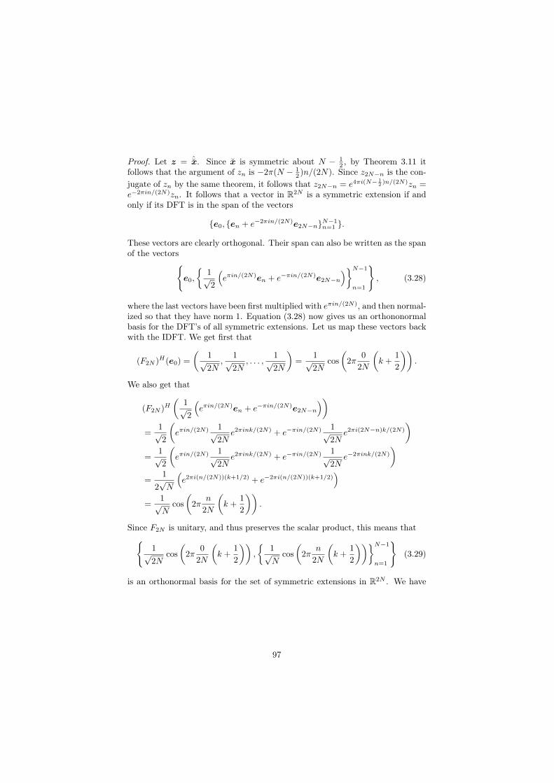
Proof. Let z = ˆ̆x. Since x̆ is symmetric about N − 12 , by Theorem 3.11 it
follows that the argument of zn is −2π(N − 12 )n/(2N). Since z2N−n is the con-
jugate of zn by the same theorem, it follows that z2N−n = e4πi(N− 12 )n/(2N)zn =
e−2πin/(2N)zn. It follows that a vector in R2N is a symmetric extension if andonly if its DFT is in the span of the vectors
{e0, {en + e−2πin/(2N)e2N−n}N−1
n=1 }.
These vectors are clearly orthogonal. Their span can also be written as the spanof the vectors
�e0,
�1√2
�eπin/(2N)
en + e−πin/(2N)e2N−n
��N−1
n=1
�, (3.28)
where the last vectors have been first multiplied with eπin/(2N), and then normal-ized so that they have norm 1. Equation (3.28) now gives us an orthononormalbasis for the DFT’s of all symmetric extensions. Let us map these vectors backwith the IDFT. We get first that
(F2N )H(e0) =
�1√2N
,1√2N
, . . . ,1√2N
�=
1√2N
cos
�2π
0
2N
�k +
1
2
��.
We also get that
(F2N )H�
1√2
�eπin/(2N)
en + e−πin/(2N)e2N−n
��
=1√2
�eπin/(2N) 1√
2Ne2πink/(2N) + e−πin/(2N) 1√
2Ne2πi(2N−n)k/(2N)
�
=1√2
�eπin/(2N) 1√
2Ne2πink/(2N) + e−πin/(2N) 1√
2Ne−2πink/(2N)
�
=1
2√N
�e2πi(n/(2N))(k+1/2) + e−2πi(n/(2N))(k+1/2)
�
=1√N
cos
�2π
n
2N
�k +
1
2
��.
Since F2N is unitary, and thus preserves the scalar product, this means that�
1√2N
cos
�2π
0
2N
�k +
1
2
��,
�1√N
cos
�2π
n
2N
�k +
1
2
���N−1
n=1
�(3.29)
is an orthonormal basis for the set of symmetric extensions in R2N . We have
97
that
S
�cos
�2π
n
2N
�k +
1
2
���
= S
�1
2
�e2πi(n/(2N))(k+1/2) + e−2πi(n/(2N))(k+1/2)
��
=1
2
�eπin/(2N)S
�e2πink/(2N)
�+ e−πin/(2N)S
�e−2πink/(2N)
��
=1
2
�eπin/(2N)λS,ne
2πink/(2N) + e−πin/(2N)λS,2N−ne−2πink/(2N)
�
=1
2
�λS,ne
2πi(n/(2N))(k+1/2) + λS,2N−ne−2πi(n/(2N))(k+1/2)
�
where we have used that e2πink/(2N) is an eigenvector of S with eigenvalueλS,n, and e−2πink/(2N) = e2πi(2N−n)k/(2N) is an eigenvector of S with eigenvalueλS,2N−n. If S preserves symmetric extensions, we see that we must have thatλS,n = λS,2N−n, and also that the vectors listed in Equation (3.29) must beeigenvectors for S. This is reflected in that the entries in D in the diagonalizationS = (F2N )HDF2N are symmetric about the midpoint on the diagonal. FromExercise 3.3.8 we know that this occurs if and only if S is symmetric, whichproves the first part of the theorem.
Since S preserves symmetric extensions it is clearly characterized by its
restriction to the first N elements. With S =
�S1 S2
S3 S4
�, we compute this
restriction as
y0...
yN−1
=�S1 S2
�
x0...
xN−1
xN
...x2N−1
=�S1 + (S2)f
�
x0...
xN−1
.
S2 contains the circulant part of the matrix, and forming (S2)f means that thecirculant parts switch corners. This shows that S is uniquely characterized bythe matrix Sr as defined in the text of the theorem. Finally, since (3.29) areeigenvectors of S, the vectors in RN restricted to their first N elements areeigenvectors for Sr. Since the scalar product of two symmetric extensions is thedouble of the scalar product of the first half of the vectors, we have that thesevectors must also be orthogonal, and that
1√N
cos
�2π
0
2N
�k +
1
2
��,
��2
Ncos
�2π
n
2N
�k +
1
2
���N−1
n=1
is an orthonormal basis of eigenvectors for Sr. We see that we now can definedn,N and the vectors dn as in the text of the theorem, and this completes theproof.
98
From the proof we clearly see the analogy between symmetric functions andvectors: while the first can be written as a cosine-series, the second can bewritten as a sum of cosine-vectors:
Corollary 3.59.
�1√2N
cos
�2π
0
2N
�k +
1
2
��,
�1√N
cos
�2π
n
2N
�k +
1
2
���N−1
n=1
�
form an orthonormal basis for the set of all symmetric vectors in R2N .
Note also that Sr is not a circulant matrix. Therefore, its eigenvectors arenot pure tones. An example should clarify this:
Example 3.60. Consider the averaging filter g = { 14 ,
12 ,
14}. Let us write down
the matrix Sr for the case when N = 4. First we obtain the matrix S as
12
14 0 0 0 0 0 1
414
12
14 0 0 0 0 0
0 14
12
14 0 0 0 0
0 0 14
12
14 0 0 0
0 0 0 14
12
14 0 0
0 0 0 0 14
12
14 0
0 0 0 0 0 14
12
14
14 0 0 0 0 0 1
412
where we have drawn the boundaries between the blocks S1, S2, S3, S4. Fromthis we see that
S1 =
12
14 0 0
14
12
14 0
0 14
12
14
0 0 14
12
S2 =
0 0 0 14
0 0 0 00 0 0 014 0 0 0
(S2)f =
14 0 0 00 0 0 00 0 0 00 0 0 1
4
.
From this we get
Sr = S1 + (S2)f =
34
14 0 0
14
12
14 0
0 14
12
14
0 0 14
34
.
The orthogonal basis we have found is given its own name:
Definition 3.61 (DCT basis). We denote by DN the orthogonal basis{d0,d1, . . . ,dN−1}. We also call DN the N -point DCT basis.
Using the DCT basis instead of the Fourier basis we can make the followingdefinitions, which parallel those for the DFT:
99

Definition 3.62 (Discrete Cosine Transform). The change of coordinatesfrom the standard basis of RN to the DCT basis DN is called the discretecosine transform (or DCT). The N×N matrix DN that represents this changeof basis is called the (N -point) DCT matrix. If x is a vector in RN , its coor-dinates y = (y0, y1, . . . , yN−1) relative to the DCT basis are called the DCTcoefficients of x (in other words, y = DNx).
As with the Fourier basis vectors, the DCT basis vectors are called synthesisvectors, since we can write
x = y0d0 + y1d1 + · · ·+ yN−1dN−1 (3.30)
in the same way as for the DFT. Following the same reasoning as for the DFT,D−1
Nis the matrix where the dn are columns. But since these vectors are real
and orthonormal, DN must be the matrix where the dn are rows. Moreover,since Theorem 3.58 also states that the same vectors are eigenvectors for filterswhich preserve symmetric extensions, we can state the following:
Theorem 3.63. DN is the orthogonal matrix where the rows are dn. More-over, for any digital filter S which preserves symmetric extensions, (DN )T
diagonalizes Sr, i.e. Sr = DT
NDDN where D is a diagonal matrix.
Let us also make the following definition:
Definition 3.64 (IDCT). We will call x = (DN )Ty the inverse DCT or(IDCT) of x.
Example 3.65. As with Example 3.9, exact expressions for the DCT can bewritten down just for a few specific cases. It turns out that the case N = 4 asconsidered in Example 3.9 does not give the same type of nice, exact values, solet us instead consider the case N = 2. We have that
D4 =
� 1√2cos(0) 1√
2cos(0)
cos�π
2
�0 + 1
2
��cos
�π
2
�1 + 1
2
���
=
�1√2
1√2
1√2
− 1√2
�
The DCT of the same vector as in Example 3.9 can now be computed as:
D2
�12
�=
�3√2
− 1√2
�.
Example 3.66. A direct implementation of the DCT could be made as follows:
function y=DCTImpl(x)
N=length(x);
DN=zeros(N);
DN(1,:)=ones(1,N)/sqrt(N);
100

for n=1:N
DN(n,:)=cos(2*pi*((n-1)/(2*N))*((0:N-1)+1/2))*sqrt(2/N);
end
y=DN*x;
In the next chapter we will see that one also can make a much more efficientimplementation of the DCT than this.
With the DCT one constructs a vector twice as long. One might think dueto this that one actually use matrices twice the size. This is, however, avoidedsince DN has the same dimensions as FN , and we will see shortly that the samealgorithms as for the DFT also can be used for the DCT. By construction wealso see that it is easy to express the N -point DCT in terms of the 2N -pointDFT. Let us write down this connection:
1. Write e0 =√2 and en = eπin/(2N) for n �= 0, and define E as the diagonal
matrix with the values e0, e1, . . . on the diagonal.
2. Let B be the 2N ×N -matrix which is nonzero only when i = j or i+ j =2N − 1, and 1 in all these places.
3. Let also A be the N × 2N -matrix with 1 on the diagonal.
We can now writeDN = E−1AF2NB. (3.31)
A here extracts the first rows of the matrix, E−1 eliminates the complex coef-ficients, while B adds columns symmetrically. This factorization enables us touse the efficient FFT-implementation, since the matrices A,B,E all are sparse.We will, however, find an even more efficient implementation of the DCT, whichwill avoid computing a DFT of twice the size as here.
Similarly to Theorem 3.16 for the DFT, one can think of the DCT as aleast squares approximation and the unique representation of a function havingthe same sample values, but this time in terms of sinusoids instead of complexexponentials:
Theorem 3.67 (Interpolation with the DCT basis). Let f be a functiondefined on the interval [0, T ], and let x be the sampled vector given by
xk = f((2k + 1)T/(2N)) for k = 0, 1, . . . , N − 1.
There is exactly one linear combination g(t) on the formN−1�
n=0
yndn,N cos(2π(n/2)t/T )
which satisfies the conditions
g((2k + 1)T/(2N)) = f((2k + 1)T/(2N)), k = 0, 1, . . . , N − 1,
and its coefficients are determined by y = DNx.
101
The proof for this follows by inserting t = (2k + 1)T/(2N) in the equationg(t) =
�N−1n=0 yndn,N cos(2π(n/2)t/T ) to arrive at the equations
f(kT/N) =N−1�
n=0
yndn,N cos
�2π
n
2N
�k +
1
2
��0 ≤ k ≤ N − 1.
This gives us an equation system for finding the yn with the invertible DCTmatrix as coefficient matrix, and the result follows.
Note the subtle change in the sample points of these cosine functions, fromkT/N for the DFT, to (2k+1)T/(2N) for the DCT. The sample points for theDCT are thus the midpoints on the intervals in a uniform partition of [0, T ] intoN intervals, while they for the DFT are the start points on the intervals. Also,the frequencies are divided by 2. In Figure 3.9 we have plotted the sinusoidsof Theorem 3.67 for T = 1, as well as the sample points used in that theorem.The sample points in (a) correspond to the first column in the DCT matrix, thesample points in (b) to the second column of the DCT matrix, and so on (up tonormalization with dn,N ). As n increases, the functions oscillate more and more.As an example, y5 says how much content of maximum oscillation there is. Inother words, the DCT of an audio signal shows the proportion of the differentfrequencies in the signal, and the two formulas y = DNx and x = (DN )Tyallow us to switch back and forth between the time domain representation andthe frequency domain representation of the sound. In other words, once we havecomputed y = DNx, we can analyse the frequency content of x. If we want toreduce the bass we can decrease the y-values with small indices and if we wantto increase the treble we can increase the y-values with large indices.
3.4.1 Other types of symmetric extensions
Note that our definition of symmetric extension duplicates the values x0 andxN−1: both are repeated when creating the symmetric extension. This is infact unnecessary when we are creating a longer vector which has equal first andlast values, and is primarily motivated from existing efficient implementationsfor the DCT when all vector lengths are powers of 2. When an efficient DCTimplementation is not important, we can change the definition of the symmetricextension as follows (it is this type of symmetric extension we will use later):
Definition 3.68 (Symmetric extension of a vector). By the symmetric exten-sion of x ∈ RN , we mean x̆ ∈ R2N−2 defined by
x̆k =
�xk 0 ≤ k < N
x2N−2−k N ≤ k < 2N − 3(3.32)
In other words, a vector in R2N is a symmetric extension of a vector in RN
if and only if it is symmetric about N − 1. Theorem 3.58 now instead takes thefollowing form:
102
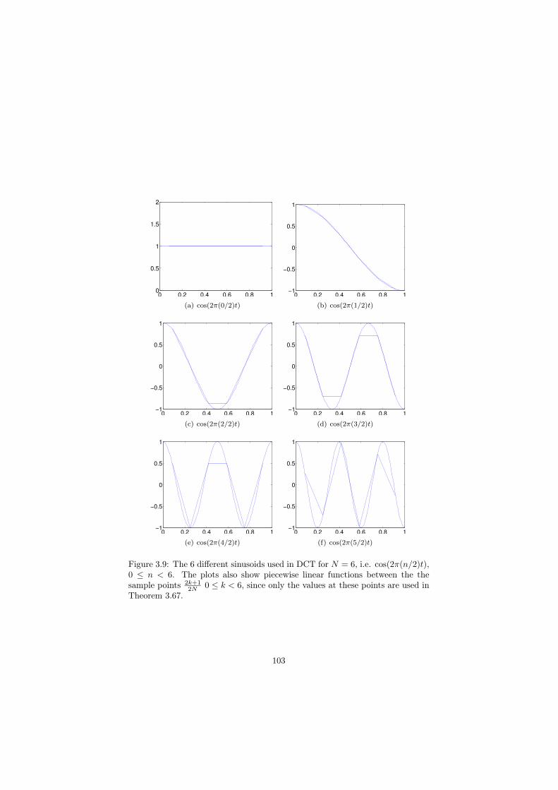
0 0.2 0.4 0.6 0.8 10
0.5
1
1.5
2
(a) cos(2π(0/2)t)
0 0.2 0.4 0.6 0.8 1!1
!0.5
0
0.5
1
(b) cos(2π(1/2)t)
0 0.2 0.4 0.6 0.8 1!1
!0.5
0
0.5
1
(c) cos(2π(2/2)t)
0 0.2 0.4 0.6 0.8 1!1
!0.5
0
0.5
1
(d) cos(2π(3/2)t)
0 0.2 0.4 0.6 0.8 1!1
!0.5
0
0.5
1
(e) cos(2π(4/2)t)
0 0.2 0.4 0.6 0.8 1!1
!0.5
0
0.5
1
(f) cos(2π(5/2)t)
Figure 3.9: The 6 different sinusoids used in DCT for N = 6, i.e. cos(2π(n/2)t),0 ≤ n < 6. The plots also show piecewise linear functions between the thesample points 2k+1
2N 0 ≤ k < 6, since only the values at these points are used inTheorem 3.67.
103

Theorem 3.69 (Characterization of filters which preserve symmetric exten-sions). A real, circulant (2N − 2)× (2N − 2)-Toeplitz matrix preverves sym-metric extensions if and only if it is symmetric. For such S, S is uniquelycharacterized by its restriction to RN , denoted by Sr, which is given by
T1 +�0 (T2)f 0
�, where T =
�T1 T2
T3 T4
�, where T1 is N × N , T2
is N × (N − 2). Moreover, an orthogonal basis of eigenvectors for Sr are{cos
�2π n
2N n�}N−1n=0 .
Proof. Let z = ˆ̆x. Since x̆ is symmetric about 0, by Theorem 3.11 it follows thatzn = z2(N−1)−n), so that the DFT of a symmetrix extension (as now defined)is in the span of the vectors
{e0, {en + e2(N−1)−n}N−1n=1 }.
It follows as before thatcos
�2π
n
2(N − 1)n
�
is a basis of eigenvectors. The same type of symmetry about the midpoint onthe diagonal follows as before, which as before is equivalent to symmetry of thematrix.
It is not customary to write down an orthonormal basis for the eigenvectorsin this case, since we don’t have the same type of efficient DCT implementationdue to the lact of powers of 2.
3.4.2 Use of DCT in lossy compression of sound
The DCT is particularly popular for processing the sound before compression.MP3 is based on applying a variant of the DCT (called the Modified DiscreteCosine Transform, MDCT) to groups of 576 (in special circumstances 192) sam-ples. One does not actually apply the DCT directly. Rather one applies a muchmore complex transformation, which can be implemented in parts by using DCTin a clever way.
We mentioned previously that we could achieve compression by setting theFourier coefficients which are small to zero. Translated to the DCT, we shouldset the DCT coefficients which are small to zero, and we apply the inverseDCT in order to reconstruct the signal in order to play it again. Let us testcompression based on this idea. The plots in figure 3.10 illustrate the principle.A signal is shown in (a) and its DCT in (b). In (d) all values of the DCT withabsolute value smaller than 0.02 have been set to zero. The signal can then bereconstructed with the inverse DCT of theorem ??; the result of this is shownin (c). The two signals in (a) and (c) visually look almost the same even thoughthe signal in (c) can be represented with less than 25 % of the informationpresent in (a).
104
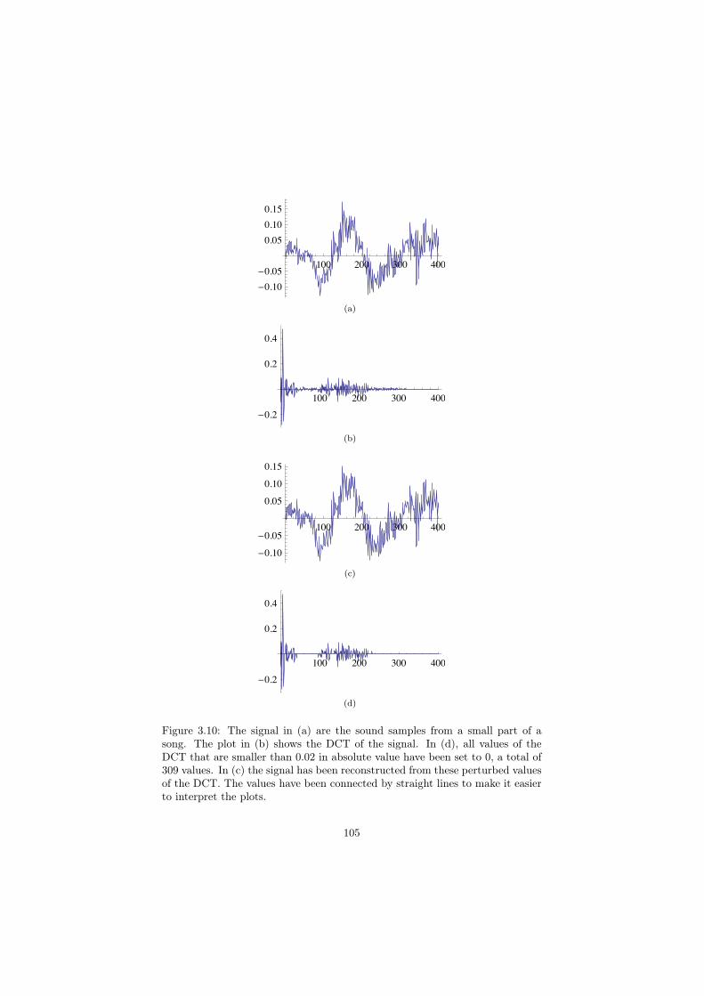
100 200 300 400
�0.10�0.05
0.050.100.15
(a)
100 200 300 400�0.2
0.2
0.4
(b)
100 200 300 400
�0.10
�0.05
0.05
0.10
0.15
(c)
100 200 300 400�0.2
0.2
0.4
(d)
Figure 3.10: The signal in (a) are the sound samples from a small part of asong. The plot in (b) shows the DCT of the signal. In (d), all values of theDCT that are smaller than 0.02 in absolute value have been set to 0, a total of309 values. In (c) the signal has been reconstructed from these perturbed valuesof the DCT. The values have been connected by straight lines to make it easierto interpret the plots.
105

We test this compression strategy on a data set that consists of 300 001points. We compute the DCT and set all values smaller than a suitable toleranceto 0. With a tolerance of 0.04, a total of 142 541 values are set to zero. Whenwe then reconstruct the sound with the inverse DCT, we obtain a signal thatdiffers at most 0.019 from the original signal. To verify that the new file isnot too different from the old file, we can take the read sound samples fromcastanets.wav, run the following function for different eps
function A=skipsmallvals(eps,A)
B=dct(A);
B=(B>=eps).*B;
A=invdct(B);
and play the new samples. Finally we can store the signal by storing a gzip’edversion of the DCT-values (as 32-bit floating-point numbers) of the perturbedsignal. This gives a file with 622 551 bytes, which is 88 % of the gzip’ed versionof the original data.
The choice of the DCT in the MP3 standard has much to do with that theDCT, just as the DFT, has a very efficient implementation, as we will see next.
Exercises for Section 3.4
Ex. 1 — In Section 3.4.2 we implemented the function skipsmallvals, whichran a DCT on the entire vector. Explain why there are less computation involvedin splitting the vector into many parts and performing a DCT for each part.Change the code accordingly.
Ex. 2 — As in Example 3.65, state the exact cartesian form of the DCT ma-trix for the case N = 3.
Ex. 3 — Assume that S is a symmetric digital filter with support [−E,E].Let us, as in Exercise 3.3.10, see how we can make sure that the indices keepinside [0, N − 1]. Show that zn = (Tx)n in this case can be split into thefollowing different formulas, depending on n:
a. 0 ≤ n < E:
zn = T0,0xn+n�
k=1
T0,k(xn+k+xn−k)+E�
k=n+1
T0,k(xn+k+xn−k+N ). (3.33)
b. E ≤ n < N − E:
zn = T0,0xn +E�
k=1
T0,k(xn+k + xn−k). (3.34)
106
c. N − F ≤ n < N :
zn = T0,0xn+N−1−n�
k=1
T0,k(xn+k+xn−k)+E�
k=N−1−n+1
T0,k(xn+k−N+xn−k).
(3.35)
Ex. 4 — Assume that {T0,−E , . . . , T0,0, . . . , T0,E} are the coefficicients of asymmetric, digital filter S, and let t = {T0,1, . . . , T0,E}. Write a function
function z=filterT(t,x)
which takes the vector t as input, and returns z = Tx using the formulasdeduced in Exercise 3.
Ex. 5 — Repeat Exercise 1.4.9 by reimplementing the functions reducetrebleand reducesbass using the function filterT from the previous exercise. Theresulting sound files should sound the same, since the only difference is that wehave modified the way we handle the beginning and end portion of the soundsamples.
Ex. 6 — Using Python, define a class Transform with methods transformImpland ItransformImpl. Define two subclasses of Transform, DCTTransform,FFTTransform), which implements these two functions by calling Python coun-terparts of FFTImpl, IFFTImpl, DCTImpl, and IDCTImpl.
3.5 Summary
We defined the Discrete Fourier transform, which could be thought of as theFourier series of a vector. We exploited properties of the DFT, which corre-sponded nicely to the corresponding properties for Fourier series. We defineddigital filters, which turned out to be linear transformations diagonalized bythe DFT. Also we showed that the techniques from the last section we used tospeed up the convergence of the Fourier series, could also be used for the DFT.In this way we arrived at the definition of the DCT.
107