doi.org/10.26434/chemrxiv.11861580.v1

Four Resonance Structures Elucidate Double-Bond Isomerisation of aBiological ChromophoreEvgeniy Gromov, Tatiana Domratcheva

Submitted date: 17/02/2020 • Posted date: 19/02/2020Licence: CC BY-NC-ND 4.0Citation information: Gromov, Evgeniy; Domratcheva, Tatiana (2020): Four Resonance Structures ElucidateDouble-Bond Isomerisation of a Biological Chromophore. ChemRxiv. Preprint.https://doi.org/10.26434/chemrxiv.11861580.v1

Photoinduced double-bond isomerisation of the chromophore of photoactive yellow protein (PYP) is highlysensitive to chromophore-protein interactions. On the basis of high-level ab initio calculations, using theXMCQDPT2 method, we scrutinise the effect of the chromophore-protein hydrogen bonds on thephotophysical and photochemical properties of the chromophore. We identify four resonance structures – twoclosed-shell and two biradicaloid – that elucidate the electronic structure of the ground and first excited statesinvolved in the isomerisation process. Changing the relative energies of the resonance structures byhydrogen-bonding interactions tunes all photochemical properties of the chromophore in an interdependentmanner. Our study sheds new light on the role of the chromophore electronic structure in tuning inphotosensors and fluorescent proteins.

File list (2)

download fileview on ChemRxivPYP-four_resonance_structures.pdf (811.56 KiB)

download fileview on ChemRxivSupporting_Information.pdf (8.40 MiB)

1

Four resonance structures elucidate double-bond

isomerisation of a biological chromophore

Evgeniy V. Gromov, and Tatiana Domratcheva

Max-Planck Institute for Medical Research, Jahnstraße 29, 69120 Heidelberg, Germany

tatjana.domratcheva@mpimf-heidelberg.mpg.de

evgeniy.gromov@mpimf-heidelberg.mpg.de

Photoinduced double-bond isomerisation of the chromophore of photoactive yellow protein (PYP)

is highly sensitive to chromophore-protein interactions. On the basis of high-level ab initio

calculations, we scrutinise the effect of the chromophore-protein hydrogen bonds on the

photophysical and photochemical properties of the chromophore. We identify four resonance

structures – two closed-shell and two biradicaloid – that elucidate the electronic structure of the

ground and first excited states involved in the isomerisation process. Changing the relative

energies of the resonance structures by hydrogen-bonding interactions tunes all photochemical

properties of the chromophore in an interdependent manner. Our study sheds new light on the role

of the chromophore electronic structure in tuning in photosensors and fluorescent proteins.

2

1. INTRODUCTION

Photoactive yellow protein (PYP)1 is a remarkable model system for studying double-bond

isomerisation in photoreceptor proteins, as this photoreceptor has amply been characterised using

a wide variety of advanced methods such as time-resolved X-ray crystallography,2-5 neutron

crystallography,6 NMR,7 and ultrafast spectroscopy.8-12 These studies provided important insights

into photoinduced double-bond isomerisation of the PYP chromophore that triggers the PYP

photoresponse. The chromophore is derived from the anionic phenolate form of the p-coumaric

thioester (pCTM−), which is in the E(trans)-configuration and stabilised by hydrogen bonds (H-

bonds) with the protein (Fig. 1a).13 The excited-state dynamics of the pCTM− anion in the protein

is different from that in solution and the gas phase.14-15 Despite numerous studies, the exact

mechanism of the protein control of the chromophore’s isomerisation remains elusive. In

particular, it is not clear how to describe the impact of the protein on the chromophore at the

electronic structure level.

The moderate molecular size and high sensitivity to intermolecular interactions render the

pCTM− chromophore (model 1 in Fig. 1b) particularly suitable for accurate quantum-chemistry

calculations addressing the chromophore’s tuning by intermolecular interactions.16-22 Similarly to

other ionic chromophores of photoresponsive proteins, pCTM− undergoes a pronounced charge-

transfer, from the phenolic moiety to the carbonyl fragment, upon photoexcitation.23 Twisting the

chromophore’s central double bond (C7=C8) or single bond (C4−C7) results in localisation of the

negative charge either on the phenolic or carbonyl moieties, respectively, in the excited (S1)

state.17, 20, 24-25 The localisation of the negative charge in the ground state (S0) is reversed to that in

the S1 state at the twisted geometries. Polar interactions of pCTM− with the protein or solvent

profoundly influence the ratio of the S1-state trajectories returning to the S0 state via the single-

3

and double-bond twists.16, 18, 24, 26 Experimentally it has been established that PYP photoactivation

is triggered by the double bond isomerisation yielding a Z(cis) isomer with a quantum yield of

0.35,27 which proceeds via a one-bond flip (OBF) mechanism destabilizing the carbonyl H-bond.2-

3, 9 Activation of the single-bond rotation has been reported for a mutated variant with weakened

phenolic H-bonds.3 The mutation leads to a slight red shift of the absorption maximum,28 reduced

charge-transfer character of the S0−S1 transition,23 and a so-called hula-twist (HT) isomerisation

combining rotations around the single and double bonds.3 In contrast to the OBF isomerisation,

the HT isomerisation preserves the carbonyl H-bond in the resulting cis photoproduct, which

impairs the signal transduction.3

Here, by performing quantum-chemistry calculations for models 1-3 (Fig. 1b) we study the

impact of H-bonds on the S0 and S1 energy at the geometries of pCTM− constituting the single and

double bond isomerisation pathways, including the geometries of the S0/S1 conical intersections

(CoIns). The accurate description of the models is attained by using a high-level ab initio method,

the extended multi-state multi-configurational quasi-degenerate perturbation theory of second

order (XMCQDPT2),29 which accounts for both static and dynamical electron correlation. In this

context, the present work critically extends the previous studies performed using the complete-

active-space self-consistent field (CASSCF) method21, 24, 30 and the single-reference second-order

approximate coupled-cluster (CC2) method.17, 20, 22, 25 To explain the trends revealed from

contrasting the three models, we deduce four resonance structures, two closed-shell (CS) and two

biradicaloid (BR), that describe charge delocalisation and charge transfer upon the S0−S1 excitation

and the bond twists. Stabilisation and destabilisation of these structures by H-bonds account for

interdependent changes of all photochemical properties of the pCTM− chromophore. We compare

our findings to previously published results on PYP, fluorescent proteins and rhodopsin

4

photoreceptors noting multiple parallels among the properties of ionic chromophore in these

proteins.

Figure 1. (a) Chromophore binding pocket (active site) of PYP featuring the anionic E(trans)-p-coumaroyl chromophore bound to PYP via a thioester linkage of the Cys69 residue and hydrogen-bonded to the backbone of Cys69 and side chains of Tyr42 and Glu46. (b) Three models considered here: the anionic p-coumaric thiomethyl (pCTM–) chromophore (1), pCTM– hydrogen-bonded with one water molecule at the carbonyl oxygen (2), mimicking the H-bond with the backbone of Cys69, and pCTM– hydrogen-bonded with two water molecules at the phenolic oxygen (3), mimicking the H-bonds with the Tyr42/Glu46 residues.

2. Computational details

The energies and geometries for models 1-3 in the S0 and S1 states were obtained from the

XMCQDPT2 calculations. As a zero-order wave function employed in the XMCQDPT2

calculations, we used a state-averaged CASSCF wave function, SA2-CASSCF(12,11). The active

space comprised 12 electrons over 11 π molecular orbitals (MOs), as previously used by Boggio-

Pasqua and Groenhof.21 The state-averaging was done for the two lowest electronic states, S0 and

5

S1, with equal weights. The subsequent XMCQDPT2 calculations using the SA2-CASSCF(12,11)

zero-order wave function further accounted for dynamical electron correlation, up to the second

order of perturbation theory, and interaction of the S0 and S1 states, via their mixing in a 2×2

Hamiltonian. The resolution of the identity (RI) approximation31-33 implemented in Firefly version

8.2 afforded a substantial speed-up of the XMCQDPT2 computations and a decrease of memory

requirements, significantly facilitating numerical evaluation of the energy gradients utilizing

supercomputer resources. An intruder state avoidance (ISA) energy shift34 of 0.02 Hartree was

applied throughout. In all our calculations, the correlation consistent double-zeta basis set of

Dunning (cc-pVDZ) was used,35-36 resulting in 231 to 277 MOs depending on the model. All MOs

were included in the MCSCF procedure, whereas the chemical-core MOs (1s of carbon and oxygen

and 1s, 2s and 2p of sulphur) were not correlated in the XMCQDPT2 calculations.

The search of stationary points on the S1 and S0 PESs and points of S1/S0 minimum energy

conical intersections (CoIn) was performed using numerical XMCQDPT2 energy gradients

computed with finite differencing of second order. In the search, internal coordinates were used

without imposing constraints, i.e, the full geometry optimisation was performed. The root mean

square (RMS) gradient for optimisation convergence was 10-3 Hartree/Bohr. In the CoIn geometry

optimisation, a penalty function method was used, with a penalty function as proposed by Martinez

and co-workers.37 The threshold of the energy gap in the CoIn optimisation was 10-3 Hartree.

Because of exceedingly high computational demands for numerical evaluation of the Hessians at

the XMCQDPT2 level, vibrational analysis at the stationary points was not performed. The type

of the stationary points was inferred based on previously published computations.17, 20 For the

saddle points, the existence of a negative curvature was confirmed by calculating relaxed energy

scans along the coordinate for which the negative curvature was expected. The planar structures

6

of models 1 and 2 (E-S1-Sad) and the single-bond twisted structure of model 3 (α-S1-Sad) were

demonstrated to correspond to saddle points by computing relaxed-energy scans along the single-

bond twisting coordinate (α-torsion). The double-bond twisted barrier (β-S1) in all the models was

demonstrated to correspond to a saddle point by computing relaxed-energy scans along the double-

bond twisting coordinate (β-torsion).

For all the stationary points, the basis set superposition error (BSSE) corrections were computed

for the S0 and S1 energies of models 2 and 3 using the protocol described in Ref 38. Overall, the

BSSE corrections for the relative/excitation energies are small, not exceeding 0.1 eV, with the

largest correction (-0.085 eV) found for the α-S1-Sad saddle point of model 3. Hereby, the

corrections for the twisted structures are larger than that for the planar structures, which obviously

relates to the different charge distribution for the planar and twisted configurations. Importantly,

accounting for the BSSE corrections does not lead to changes in the relative order of the stationary

points, either within a particular model or the different models. In the following, we therefore

neglect the BSSE corrections, presenting and discussing the plain XMCQDPT2 results.

Oscillator strengths, Mulliken atomic charges and free valences on atoms (number of unpaired

electrons)39 were computed using the S0 and S1 zero-order QDPT electron densities. For analysis

of the S0 and S1 PESs in the vicinity of CoIn, an approach suggested by Olivucci and co-workers

was used.40-41 A series of points circumscribing a CoIn point (loops) lying in the branching plane

were computed. The branching plane is defined by the gradient difference (x1) and derivative

coupling (x2) vectors.42 We computed the x1 and x2 vectors with the SA2-CASSCF(12,11) method

using Gaussian09,43 with solving the coupled-perturbed equations in the MCSCF cycle being

skipped (“nocpmcscf” approximation).44 The error introduced by the latter decreases with the

decrease of the S0−S1 energy gap; therefore it might be important at the Frank-Condon region and

7

negligible at CoIn. Except computations of the branching vectors, all calculations were performed

using version 8.2 of the Firefly quantum chemistry package,45 which is partially based on the

Gamess-US source code.46 The computations utilised resources of the high performance

computing cluster JURECA.47

3. RESULTS AND DISCUSSION

3.1. Characterisation of single- and double-bond twists

Figure 2 depicts cross-sections through the S0 and S1 potential energy surfaces (PESs) computed

for models 1-3 along the single- and double-bond twisting pathways starting from the E(trans) S0

minimum (E-S0-Min). For each model, the cross-section is composed of several stationary points

on the S0 and S1 PESs and points of S1/S0 minimum-energy conical intersections (CoIns).

Specifically, there are the E(trans) and Z(cis) planar minima in the ground S0 state, two minima

and two saddle points of planar and twisted geometries in the S1 state, and two twisted CoIn points.

All the points were obtained from a full geometry optimisation using the XMCQDPT2 method. In

the following, we refer to the rotation around the C4−C7 bond as α-twist and around the C7−C8

bond as β-twist (Fig. 1b) according to the previously adopted notation. 17, 20, 25 The geometries of

the models at the stationary points are depicted in Fig. S1 in the Supporting Information (SI). The

energies given in Fig. 2 are not corrected for the basis set superposition error (BSSE), which

according to our estimation introduces only marginal changes in the cross-section energies (Table

S3 in SI).

8

Figure 2. Cross-sections of S0 and S1 PESs for models 1 (blue), 2 (green) and 3 (red) for the photoinduced α and β twisting. The following notations are used to indicate the geometry and type of the stationary points. Planar ground-state minima featuring E(trans) and Z(cis) configurations with respect to the central −C7=C8− double bond, E-S0-Min and Z-S0-Min, respectively; planar excited-state saddle point and minimum, E-S1-Sad and E-S1-Min, respectively; α-twisted excited-state minimum and saddle point, α-S1-Min and α-S1-Sad, respectively; α-twisted CoIn, α-CoIn; β-twisted saddle point, β-S1-Sad; β-twisted minimum, β-S1-Min; β-twisted CoIn, β-CoIn. All geometries are shown in Fig. S1 in SI. The total and relative energies of the points are listed in Tables S1-S2 in SI.

At first, we consider the results for model 1, which relate to the intrinsic properties of the pCTM−

chromophore (blue cross-section in Fig. 2). At the trans configuration E-S0-Min minimum, the

S0−S1 vertical excitation energy (VEE) is 2.60 eV and the corresponding oscillator strength is close

to unity From the Franck-Condon (FC) point, the chromophore first undergoes a bond-length

alteration (BLA) geometry relaxation toward the planar E-S1-Sad saddle point followed by the α-

twist relaxation toward the 90°-twisted α-S1-Min minimum. Structurally close to the α-S1

minimum but higher in energy, there is a S1/S0 α-CoIn, mediating decay of the excited-state

population back to the S0 state. The excited-state α-twist was previously implicated in internal

conversion.20, 22, 24 Activation of the β-twist involves passing a small barrier, β-S1-Sad, which is

0.12 eV above VEE, and is associated with the change of the BLA coordinate and β torsion.

9

Beyond the barrier, the chromophore relaxes by undergoing further β-twist toward the 90°-twisted

β-S1-Min minimum. Structurally close to the β-S1 minimum but higher in energy, there is a S1/S0

β-CoIn, through which the chromophore decays back to the S0 state either forward to the Z-S0-Min

minimum or backward to the E-S0 minimum. The ratio of the Z and E products depends on many

factors, one of which is the topology of the S0 PES in the vicinity of β-CoIn. Both the α- and β-

CoIns demonstrate a sloped topology, as each of them was found in the vicinity of a 90°-twisted

S1 energy minimum.

The results of models 2 and 3 (green and red cross-sections, respectively, in Fig. 2) demonstrate

that the H-bonds lead to considerable energy changes and, moreover, to a change of the S1 PES

topology in the case of model 3. Specifically, the carbonyl H-bond in 2 reduces VEE, stabilises

the α-pathway and destabilises the β-pathway. In contrast, the phenolic H-bonds in 3 increase

VEE, destabilise the α-twist and stabilises the β-twist. Notably, the α-twist energies are more

affected by the H-bonds than that of the β-twist. In 3, destabilisation of the α-twist results in

appearance of the planar E-S1-Min minimum, with the α-S1 α-twisted geometry becoming a saddle

point (red cross-section in Fig. 2).

3.2. Four resonance structures rationalizing effect of H-bonds

In the previous studies, the effect of the H-bonds on the S0 and S1 energies has been explained by

stabilisation and destabilisation of the negative charge either on the phenolic or carbonyl groups

of pCTM−.17, 20, 24-25 At the planar E-S0 minimum, the charge de-localisation is explained by the

resonance of two closed-shell (CS) anionic forms.17, 25 At the same time, the origin of the reversed

negative charge localisation at the α- and β-twisted S1 minima has not been linked to any resonance

forms so far.17, 20, 25 To elucidate this issue, we analyzed distribution of the negative charge and

10

the number of unpaired electrons (NUE)39 at the different geometries (stationary points) in the S0

and S1 state (Fig. 3, Tables S5-S7 in SI). The analysis indicates that the S0−S1 electronic excitation

results in a significant charge transfer and increase of NUE, which is consistent with a biradicaloid

(BR) structure of the S1 state (Table S8 in SI). The key result of our analysis is realizing that the

changes of the phenolic charge and NUE at all the stationary points (Fig. 3) can be accounted for

by changing contributions of four resonance structures − two CS structures, characterizing the S0

state as mentioned above, and two BR structures, characterizing the S1 state (Scheme 1). The

resonance structures are denoted according to the presence of the phenolic (Ph) or quinonic (Qn)

π-system. Noteworthy, QnBR relates to PhCS, and PhBR relates to QnCS via an electron

excitation. Precisely, QnBR describes a single-electron charge-transfer excitation of PhCS,

whereas PhBR describes a single-electron charge-transfer excitation of QnCS. To the best of our

knowledge, the QnBR and PhBR structures have never been explicitly considered for pCTM−

before.

It is worth noting that the four resonance structures are consistent with those introduced in the

biradicaloid theory of Bonačić-Koutecký et al.48-49 and theory of twisted intermolecular charge-

transfer (TICT) of Rettig and co-workers.50-51 The TICT theory treats the “hole-pair” (hp)

configuration of a polar chromophore as electron-acceptor and electron-donor moieties connected

via a central single bond. The electron transfer from the donor to the acceptor upon the HOMO-

LUMO excitation (typically corresponding to the S0−S1 transition) yields a “dot-dot” (dd) structure

with a translocated molecular charge. By twisting the linking single bond, the HOMO and LUMO

involved in the charge-transfer transition become localised on the mutually orthogonal molecular

fragments, and thus do not interact. Therefore, the twisting decreases the energy of the dd

11

configuration and increases the energy of the hp configuration, which altogether significantly

reduces the S0−S1 energy difference and even leads to S0/S1 state crossing.48, 51

Figure 3. Distribution of (a) the net negative charge on the phenolic moiety in the S0 and S1 states and (b) the number of unpaired electrons (NUE) at the C4, C7 and C8 atoms in the S1 state in models 1-3 at the different stationary points along the α- and β-twisting pathways. The colour code is the same as in Fig. 2. The atomic and net charges on the phenolic and carbonyl moieties, as well as NUE are given in Tables S5-S7 in SI.

12

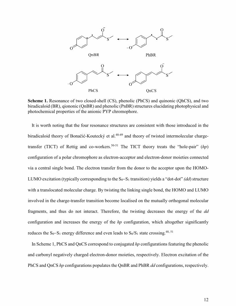
Scheme 1. Resonance of two closed-shell (CS), phenolic (PhCS) and quinonic (QhCS), and two biradicaloid (BR), qiononic (QnBR) and phenolic (PnBR) structures elucidating photophysical and photochemical properties of the anionic PYP chromophore.

It is worth noting that the four resonance structures are consistent with those introduced in the

biradicaloid theory of Bonačić-Koutecký et al.48-49 and theory of twisted intermolecular charge-

transfer (TICT) of Rettig and co-workers.50-51 The TICT theory treats the “hole-pair” (hp)

configuration of a polar chromophore as electron-acceptor and electron-donor moieties connected

via a central single bond. The electron transfer from the donor to the acceptor upon the HOMO-

LUMO excitation (typically corresponding to the S0−S1 transition) yields a “dot-dot” (dd) structure

with a translocated molecular charge. By twisting the linking single bond, the HOMO and LUMO

involved in the charge-transfer transition become localised on the mutually orthogonal molecular

fragments, and thus do not interact. Therefore, the twisting decreases the energy of the dd

configuration and increases the energy of the hp configuration, which altogether significantly

reduces the S0−S1 energy difference and even leads to S0/S1 state crossing.48, 51

In Scheme 1, PhCS and QnCS correspond to conjugated hp configurations featuring the phenolic

and carbonyl negatively charged electron-donor moieties, respectively. Electron excitation of the

PhCS and QnCS hp configurations populates the QnBR and PhBR dd configurations, respectively.

13

At the same time, the α- (β-) twist leads to the QnBR (PhBR) structure in the S1 state, and the

PhCS (QnCS) structure in the S0 state. This picture is fully confirmed by Fig 4, which displays the

difference of the S1 and S0 total electron densities at the α-S1 and β-S1 twisted minima. As can be

clearly seen in the figure, the negative charge at the α-S1 minimum resides on the alkene-carbonyl

fragment in the S1 state and on the phenolic fragment in the S0 state (Fig. 4a), whereas it is vice

versa at the β-S1 minimum (Fig. 4b). The same holds for models 2 and 3.

Figure 4. Difference of the S1 and S0 electron densities at the α-twisted (a) and β-twisted (b) minima of pCTM− (model 1). Orange and purple correspond to S1 and S0 electron densities, respectively.

Resonance of the PhCS and QnCS structures determines the single- and double-bond lengths at

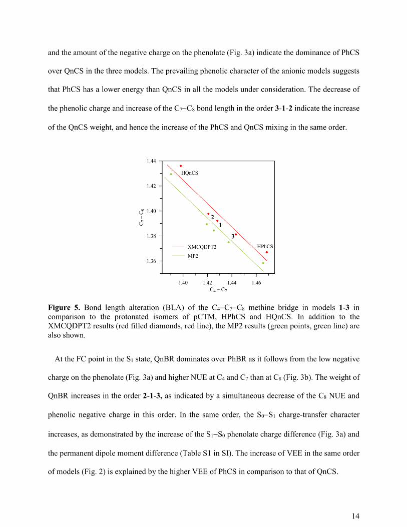
the planar E-S0-Min minimum and the charge distribution in the S0 state. Figure 5 shows the BLA

of the C4−C7−C8 methine bridge in the anionic models in comparison to that in the protonated

phenol and enol isomers of pCTM. The shorter C7−C8 distance in comparison to C4−C7 (Fig. 5)

14

and the amount of the negative charge on the phenolate (Fig. 3a) indicate the dominance of PhCS

over QnCS in the three models. The prevailing phenolic character of the anionic models suggests

that PhCS has a lower energy than QnCS in all the models under consideration. The decrease of

the phenolic charge and increase of the C7−C8 bond length in the order 3-1-2 indicate the increase

of the QnCS weight, and hence the increase of the PhCS and QnCS mixing in the same order.

Figure 5. Bond length alteration (BLA) of the C4−C7−C8 methine bridge in models 1-3 in comparison to the protonated isomers of pCTM, HPhCS and HQnCS. In addition to the XMCQDPT2 results (red filled diamonds, red line), the MP2 results (green points, green line) are also shown.

At the FC point in the S1 state, QnBR dominates over PhBR as it follows from the low negative

charge on the phenolate (Fig. 3a) and higher NUE at C4 and C7 than at C8 (Fig. 3b). The weight of

QnBR increases in the order 2-1-3, as indicated by a simultaneous decrease of the C8 NUE and

phenolic negative charge in this order. In the same order, the S0−S1 charge-transfer character

increases, as demonstrated by the increase of the S1−S0 phenolate charge difference (Fig. 3a) and

the permanent dipole moment difference (Table S1 in SI). The increase of VEE in the same order

of models (Fig. 2) is explained by the higher VEE of PhCS in comparison to that of QnCS.

15

Thus, mixing of PhCS and QnCS determines de-localisation of the molecular charge in the S0

state, the extent of BLA at the S0 equilibrium geometry, the S0−S1 VEE and the extent of the charge

transfer upon S0−S1 excitation. Obviously, the more PhCS prevails in the S0 state (small

PhCS/QnCS mixing), the larger the BLA and phenolic charge in the S0 state and the larger the

S0−S1 VEE and the extent of the charge-transfer. In contrast, the less the PhCS prevails in the S0

wave function (large PhCS/QnCS mixing), the smaller the BLA and phenolic charge in the S0

state, and the smaller the S0−S1 VEE and the charge-transfer upon excitation.

3.3 Energies of the resonance structures − impact on the S1 state and S1/S0 conical

intersections

The energies of the resonance structures can be estimated for the 90°-twisted geometries.52 Indeed,

the four resonance structures are uncoupled at the α-S1 and β-S1 twisted minima, with the negative

charge being completely localised either on the phenolic or carbonyl fragment, as evident in Fig

3a. At the α-S1 minimum, the S0 state corresponds to the PhBR structure, whereas the S1 state is

represented by the QnBR structure, with the negative charge being localised on the phenolic

moiety and carbonyl fragment in the S0 and S1 states, respectively (Fig. 3a and 4a), and the C8

NUE has the smallest value (Fig. 3b). At the β-S1 minimum, the S0 state is represented by the

QnCS structure, while the S1 state is associated with the QnBR structure, with the negative charge

being localised on the carbonyl fragment and phenolic moiety in the S0 and S1 states, respectively

(Fig. 3a and 4b), and the C8 NUE has the largest value (Fig. 3b).

By comparing the energies at the 90°-twisted geometries (Fig. 2), we infer that PhCS has the

lowest energy among the four resonance structures in all the models, which is in agreement with

the analysis of the resonance mixing at the planar geometries described above. The carbonyl H-

16

bond stabilises QnCS and QnBR and destabilises PhCS and PhBR, whereas the phenolic H-bonds

stabilise PhCS and PhBR and destabilise QnCS and QnBR. Among the four resonance forms, the

energy of QnBR demonstrates the largest variation due to the H-bonding interactions.

As the geometries of the stationary points demonstrate, the BLA, α-twist and β-twist are the

main coordinates driving the relaxation of the pCTM− chromophore in the S1 excited state. If the

QnBR energy is lower than VEE, the initial relaxation from the FC point involves the BLA

coordinate followed by the α-twist. If that condition is not fulfilled, which is the case for model 3

(see Fig.2), the planar E-S1 minimum appears on the S1 PES.

At the planar E-S1-Min minimum (model 3), the S0−S1 oscillator strength is 0.9, and the

computed radiative rate is ~0.26 ns-1, suggesting a sizable emission with a Stokes shift defined by

the extent of the BLA relaxation. At the twisted α-S1 minimum in models 1 and 2, the computed

radiative rate is several orders of magnitude smaller, ~0.51 s-1, because of the substantial decrease

of the S0−S1 energy and oscillator strength. Based on these results, we predict that the dynamics

of the fluorescence signal in PYP correlates with the dynamics of the chromophore H-bonds

stabilizing/destabilizing the planar E-S1 minimum. The smaller BLA variation at the planar S1

minimum as compared to that at the S0 minimum is a consequence of the chromophore instability

with respect to the α-twist. As the α-twist virtually quenches the fluorescence, the variation of the

emission maximum in colour-tuned PYP mutants should be significantly smaller than that of the

absorption maximum, which indeed was experimentally observed by Hoff and co-workers.28

Finally, the energies of the resonance structures at the α-S1 and β-S1 minima determine the

energies of α-CoIn and β-CoIn, which in turn define whether the excited chromophore returns to

the S0 state via a single- or double-bond twist. As Fig 2 demonstrates, the CoIn energies correlate

with the S0−S1 energy gap at the 90°-twisted geometries, i.e., the difference in energy of the

17

corresponding CS and BR resonance structures. The smaller the energy gap at the 90°-twisted S1

minimum (or saddle point), the lower the CoIn energy and the smaller the distortion of the CoIn

geometry in comparison to the twisted minimum (or saddle point). As an example, we consider

model 3, for which the PhCS and QnBR energy difference is rather high, and consistently the high-

energy α-CoIn in this model demonstrates a substantial β-twist in addition to the α-twist (Fig. S1

in SI). In contrast, stabilisation of PhBR and destabilisation of QnCS by the phenolic H-bonds

lowers the energy of the β-CoIn and reduces its distortion with respect to the β-S1 minimum. In

models 1 and 2, the PhCS and QnBR energy difference is smaller than in model 3, the α-CoIn

energy therefore decreases, whereas the PhBR and QnCS energy difference is larger, and hence

the β-CoIn energy increases. The variations of the α-CoIn energy among the models suggests that

accessibility of α-CoIn and therefore activation of the single bond rotation and internal conversion

via the single-bond twist can be efficiently controlled by chromophore-protein interactions.

Stabilisation of PhCS and PhBR by these interactions reduces the resonance mixing and favours

the double-bond OBF isomerisation.

3.4 Double-bond isomerisation of the pCTM− chromophore

The β-CoIn provides the excited-state decay channel for the OBF double-bond isomerisation of

pCTM−. We remind that a minimum energy CoIn geometry corresponds to a local energy

minimum on the 3N-8 dimensional hypersurface (N is the number of atoms) where the S1 and S0

states are degenerate.42 The degeneracy is lifted in the first order along the gradient difference

vector (x1) and the derivative coupling vector (x2), forming a so-called branching plane.53-55

Inspection of the energies in the branching plane unveils relaxation on the S0 PES after a non-

adiabatic S1-S0 transition at the β-CoIn. We computed x1 and x2 at the β-CoIn geometries and

18

constructed branching-plane loops following the procedure suggested by Olivucci and co-

workers.56 In all our models, x1 is dominated by BLA, whereas x2 features the β-torsion and, in

addition, hydrogen out-of-plane (HOOP)20, 22, 57 excursions, which mix with the BLA changes in

models 1 and 2 (see Fig. S2 in SI). At the β-CoIn geometries, the HOOP value tends to be “ahead”

of β-torsion, i.e., smaller than β-torsion, when β > 90° (in models 1 and 2), whereas it is

“concerted” with β-torsion (close to β-torsion) when β < 90° (model 3) (Fig. S3 in SI). Fig. 6a

presents the x1 and x2 vectors for model 3 (for the other models see Fig. S2 in SI). Fig. 6b

demonstrates that β-CoIn has the β-torsion value slightly smaller than 90° in model 3, whereas it

shifts toward a larger β-torsion value (i.e., closer to the initial E(trans) geometry) in models 1 and

2. The smaller β-torsion value at the β-CoIn, explained by stabilisation of PhBR and destabilisation

of QnCS in model 3, is favourable for the E(trans)-Z(cis) isomerisation. The β-CoIn branching

plane of pCTM− is similar to that previously reported for the double-bond isomerisation of the

retinal protonated Schiff base (RPSB) chromophore and analogues in rhodopsins.58-59

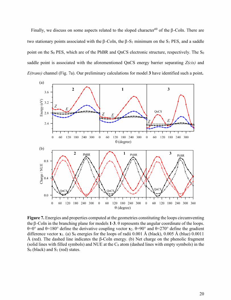
Figure 7 shows the energy and property changes along the branching plane loops. In the x1

direction (θ=90°, 270°), the S0 and S1 wave functions change from one resonance structure to

another. Specifically, the charge distribution and NUE (Fig. 7b) indicate that the S0 wave function

changes from QnCS to PhBR whereas the S1 wave function changes from PhBR to QnCS. The x2

direction (θ=0°,180°) corresponds to mixing of PhBR and QnCS and, to a lesser extent, of PhCS,

as indicated by the changes of the phenolic charge and NUE (Fig. 7b). The presence of PhCS

follows from the steeper phenolic charge curve in comparison to the NUE curve. The PhCS weight

significantly increases as the chromophore becomes more planar.

Two S0 energy minima emerge along x2 (Fig. 7a) as decay channels towards the Z(cis) and

E(trans) minima. Notably, the Z(cis) decay channel lies below the β-CoIn energy only in 3 (at

19

θ=0°, Fig. 7a), correlating with the smaller β-torsion value at β-CoIn in this model. In addition,

there is a high-energy barrier, associated with the QnCS structure, separating the two channels in

model 3, which is explained by the higher QnCS energy in this model. Overall, the topology of the

S0 PES along the loops suggests that the double-bond isomerisation quantum yield is higher in 3

as compared to 1 and 2.

Figure 6. Characterisation of the β-twisted CoIn: (a) The branching plane vectors x1 and x2 for model 3 (see also Fig. S2 presenting x1 and x2 for all three models) (b) Changes in the β-torsion and C7=C8 bond length along the 0.005-Å loops for models 1-3. The values of the angular coordinate θ at some points of the loops, and the orientation of the x1 and x2 vectors are indicated. The colour code is the same as in Fig. 2.

20

Finally, we discuss on some aspects related to the sloped character60 of the β-CoIn. There are

two stationary points associated with the β-CoIn, the β-S1 minimum on the S1 PES, and a saddle

point on the S0 PES, which are of the PhBR and QnCS electronic structure, respectively. The S0

saddle point is associated with the aforementioned QnCS energy barrier separating Z(cis) and

E(trans) channel (Fig. 7a). Our preliminary calculations for model 3 have identified such a point.

Figure 7. Energies and properties computed at the geometries constituting the loops circumventing the β-CoIn in the branching plane for models 1-3. θ represents the angular coordinate of the loops. θ=0° and θ=180° define the derivative coupling vector x2. θ=90° and θ=270° define the gradient difference vector x1. (a) S0 energies for the loops of radii 0.001 Å (black), 0.005 Å (blue) 0.0011 Å (red). The dashed line indicates the β-CoIn energy. (b) Net charge on the phenolic fragment (solid lines with filled symbols) and NUE at the C8 atom (dashed lines with empty symbols) in the S0 (black) and S1 (red) states.

21

This is the only saddle point connecting the Z(cis) and E(trans) minima on the S0 PES, and hence

it mediates the thermal isomerisation. The sloped type of β-CoIn implies that the aforementioned

two stationary points lie on the same side from the β-CoIn along x1. This is different from the

peaked CoIn found for the RPSB chromophore and its analogues, where two saddle points of

different electronic structure lying on the S0 PES flank the CoIn along the BLA coordinate.61-64

Noteworthy, for the rhodopsin photoreceptor, the energy of the saddle point controlling the thermal

isomerisation was found to correlate with VEE, such that the blue-shifted absorption maximum

corresponds to a reduced thermal activation (higher energy of the saddle points).61 Despite

different β-CoIn topology, a similar correlation as for the RPSB chromophore should be expected

for the pCTM− chromophore, as the increase of VEE correlates with the increase of the QnCS

energy.

3.5 Comparison to other computational studies

Although our models 1-3 do not account for the real environment of the pCTM− chromophore in

PYP, they correctly grasp the effects of the Cys69 and Tyr42/Glu46 H-bonds (Fig. 1a). The energy

changes presented in Fig. 2 are qualitatively consistent with those predicted by the hybrid

quantum-mechanics/molecular mechanics (QM/MM) models of PYP16, 18-19, 26 and solvated

chromophore.24 Specifically, the carbonyl H-bond lowers the α-CoIn energy, whereas the phenolic

H-bonds lower the β-CoIn energy in the QM/MM models.24 In the surface-hopping molecular

dynamics simulations of PYP,26 the presence of the protonated (positively charged) Arg52

stabilizing the phenolic negative charge, that is the PhCS and PhBR resonance structures with

respect to the QnCS and QnBR ones, leads to stabilisation of the β-CoIn, and hence facilitates the

OBF isomerisation.

22

We compare the energies of model 1 with the results of Boggio-Pasqua and Groenhof21 obtained

using the CASSCF(12,11) method, and the energies of model 3 with the results of Gromov et al.17,

20 obtained using the CC2 method. It is instructive to consider the energies of the resonance

structures at the 90°-twisted geometries. Both CC2 and CASSCF favour QnBR over PhBR more

than predicted by the XMCQDPT2 method. Consistent with this energy trend, the β-CoIn is higher

in energy than α-CoIn at the CASSCF level of theory, whereas it is vice versa at the XMCQDPT2

level. Thus, employing the CASSCF method to describe the pCTM− chromophore in surface-

hopping dynamics of PYP16, 26 underestimates the efficiency of the β-twist in the S1 state. For a

similar anionic chromophore of the green fluorescent proteins (GFPs), it has indeed been reported

that the CASSCF method underestimates the decay of the S1 state via the β-twist as compared to

the more accurate XMSCASPT2 method.65 In the QM/MM simulations of PYP,26 this

underestimation seems to be compensated by the effect of the positively charged residues, such as

protonated Arg52 stabilizing, the PhCS and PhBR structures.

3.6 Similarity with other biological chromophores

Similar to pCTM−, the anionic p-hydroxybenzylideneimidazolinole (pHBDI−) chromophore of

GFPs is described by resonance interactions of the PhCS and QnCS forms coupled along the BLA

reaction coordinate.66-67 Recently, Boxer and co-workers67 suggested that the energy difference of

the PhCS and QnCS forms can serve as a linear scale for quantitative prediction of the GFP

photophysical properties using a small number of parameters intrinsic to the pHBDI−

chromophore. This energy difference was implicated to explain all strong correlations of properties

among a large number of systematically tuned GFP variants.67 We note that the charge-transfer

GFP model of Boxer and co-workers67 is consistent with our computational results for the anionic

23

pCTM− except that it does not invoke the QnBR and PhBR structures of pHBDI−. By analogy to

pCTM−, we suggest that the energies and properties of the QnBR and PhBR resonance forms

should be considered when addressing the S1 PES of pHBDI− in GFPs, in particular its

photoactivation. Applying this prediction, stabilisation of PhBR in pHBDI− favours the OBF

double-bond isomerisation, whereas stabilisation of QnBR gives a chance to the single-bond

activation and HT isomerisation.68

Mixing of the resonance forms describes charge delocalisation in protonated cationic

chromophores such as the RPSB chromophore of rhodopsins and tetrapyrrole chromophores of

phytochromes. The extent of mixing explains different sensitivities of these chromophores to

electrostatic interactions with their proteins. The dominant resonance structure of RPSB features

a positive charge localised on the Schiff-base fragment, giving rise to considerable charge-transfer

character of the S0−S1 transition and high sensitivity to electrostatic interactions with the protein.

These interactions in turn, efficiently control the contributions of the resonance forms, as suggested

by the correlations of the increased/decreased BLA and increased/decreased VEE.69-71 In contrast,

the tetrapyrrole positive charge is redistributed among the four pyrrole rings described by at least

four resonance forms.72 This charge delocalisation reduces the charge-transfer character of the

S0−S1 transition and subsequently reduces the electrostatic effect of the protein on the

chromophore.

4. CONCLUSIONS AND OUTLOOK

Given the prominent role of ionic chromophores in light activation of naturally evolved

photoreceptor proteins, it is important to rationalise the effect of chromophore-protein interactions

that are crucial for the light sensory function. Here, by analysing how the anionic pCTM−

24

chromophore of the PYP bacterial photoreceptor is influenced by phenolic or carbonyl H-bonds

we derived a qualitative model explaining interdependent changes of all photochemical properties

related to the PYP photoactivation. To account for electronic correlation effects, the state-of-the-

art XMCQDPT2 method was employed to compute the S0 and S1 PES cross-sections. To

rationalise the obtained trends, two pairs of resonance structures, each pair comprised of a CS

structure and corresponding to it charge-transfer BR structure were invoked (Scheme 1).

Delocalisation of the negative charge and other properties of the S0 and S1 states are described by

chemical resonance of the structures with the opposite charge localisation. Contributions of the

resonance structures depend on their energies that we compare at the 90° single- and double-bond

twisted geometries where chemical resonance vanishes.

From the computational results, the following picture of tuning pCTM− by intermolecular

interactions emerges. Stabilisation of the phenolic CS and BR structures by the phenolic H-bonds

leads to the larger difference in the lengths of the central single and double bonds (i.e. larger BLA)

at the S0 minimum-energy geometry; there is also an increase of the excitation energy and

stabilisation of the planar S1 minimum. Moreover, isomerisation around the central double bond

becomes more favourable than the phenolic ring rotation around the single bond, and the energy

barrier controlling the thermal double-bond isomerisation increases. In contrast, stabilisation of

the quinonic structures by the carbonyl H-bond leads to delocalisation of the negative charge and

a smaller BLA in the S0 state, smaller S0−S1 excitation energy and smaller charge transfer

character, as well as activation of the single-bond rotation in the S1, increasing the probability of

the HT photoisomerisation. Overall, our computational results predict that stabilisation of the

pCTM− phenolic resonance structures, i.e. reduction of chemical resonance, is crucial for PYP

photoactivation via the OBF double-bond isomerisation.

25

Comparison of our findings and conclusions to the previously published computational and

theoretical results characterizing other biological chromophores identifies many common features.

In particular, our model derived from the high-level quantum-chemistry calculations in its essence

is similar to a model proposed by Boxer and co-workers67, 73 explaining spectral properties of

systematically mutated GFP proteins. Yet, our model extends Boxer’s model to the twisted

geometries and invokes BR structures to describe the S1 state properties. The broad similarities

among the ionic chromophores imply that the concept of chemical resonance is instructive in

experimental and especially computational studies addressing photochemical mechanisms of

photosensory proteins operating via the double-bond isomerisation.

ACKNOWLEDGEMENTS

We would like to dedicate this paper to the memory of Alex. A. Granovsky, an inspired scientist

and the principal developer of the Firefly quantum chemistry program package, who developed

and implemented the XMCQDPT2 method, and made other valuable contributions in quantum

chemistry. The computing time granted by the John von Neumann Institute for Computing (NIC)

on the supercomputer JURECA at Jülich Supercomputing Centre (JSC) is gratefully

acknowledged.

26

REFERENCES

1. Hellingwerf, K. J.; Hendriks, J.; Gensch, T., Photoactive Yellow Protein, a new type of photoreceptor protein: Will this "yellow lab" bring us where we want to go? J Phys Chem A 2003, 107 (8), 1082-1094.

2. Schotte, F.; Cho, H. S.; Kaila, V. R.; Kamikubo, H.; Dashdorj, N.; Henry, E. R.; Graber, T. J.; Henning, R.; Wulff, M.; Hummer, G.; Kataoka, M.; Anfinrud, P. A., Watching a signaling protein function in real time via 100-ps time-resolved Laue crystallography. Proc Natl Acad Sci U S A 2012, 109 (47), 19256-61.

3. Jung, Y. O.; Lee, J. H.; Kim, J.; Schmidt, M.; Moffat, K.; Srajer, V.; Ihee, H., Volume-conserving trans-cis isomerization pathways in photoactive yellow protein visualized by picosecond X-ray crystallography. Nat Chem 2013, 5 (3), 212-20.

4. Tenboer, J.; Basu, S.; Zatsepin, N.; Pande, K.; Milathianaki, D.; Frank, M.; Hunter, M.; Boutet, S.; Williams, G. J.; Koglin, J. E.; Oberthuer, D.; Heymann, M.; Kupitz, C.; Conrad, C.; Coe, J.; Roy-Chowdhury, S.; Weierstall, U.; James, D.; Wang, D.; Grant, T.; Barty, A.; Yefanov, O.; Scales, J.; Gati, C.; Seuring, C.; Srajer, V.; Henning, R.; Schwander, P.; Fromme, R.; Ourmazd, A.; Moffat, K.; Van Thor, J. J.; Spence, J. C.; Fromme, P.; Chapman, H. N.; Schmidt, M., Time-resolved serial crystallography captures high-resolution intermediates of photoactive yellow protein. Science 2014, 346 (6214), 1242-6.

5. Pande, K.; Hutchison, C. D.; Groenhof, G.; Aquila, A.; Robinson, J. S.; Tenboer, J.; Basu, S.; Boutet, S.; DePonte, D. P.; Liang, M.; White, T. A.; Zatsepin, N. A.; Yefanov, O.; Morozov, D.; Oberthuer, D.; Gati, C.; Subramanian, G.; James, D.; Zhao, Y.; Koralek, J.; Brayshaw, J.; Kupitz, C.; Conrad, C.; Roy-Chowdhury, S.; Coe, J. D.; Metz, M.; Xavier, P. L.; Grant, T. D.; Koglin, J. E.; Ketawala, G.; Fromme, R.; Srajer, V.; Henning, R.; Spence, J. C.; Ourmazd, A.; Schwander, P.; Weierstall, U.; Frank, M.; Fromme, P.; Barty, A.; Chapman, H. N.; Moffat, K.; van Thor, J. J.; Schmidt, M., Femtosecond structural dynamics drives the trans/cis isomerization in photoactive yellow protein. Science 2016, 352 (6286), 725-9.

6. Yonezawa, K.; Shimizu, N.; Kurihara, K.; Yamazaki, Y.; Kamikubo, H.; Kataoka, M., Neutron crystallography of photoactive yellow protein reveals unusual protonation state of Arg52 in the crystal. Sci Rep 2017, 7 (1), 9361.

7. Sigala, P. A.; Tsuchida, M. A.; Herschlag, D., Hydrogen bond dynamics in the active site of photoactive yellow protein. P Natl Acad Sci USA 2009, 106 (23), 9232-9237.

8. Larsen, D. S.; van Grondelle, R., Initial photoinduced dynamics of the photoactive yellow protein. Chemphyschem 2005, 6 (5), 828-837.

9. van Wilderen, L. J.; van der Horst, M. A.; van Stokkum, I. H.; Hellingwerf, K. J.; van Grondelle, R.; Groot, M. L., Ultrafast infrared spectroscopy reveals a key step for successful entry into the photocycle for photoactive yellow protein. Proc Natl Acad Sci U S A 2006, 103 (41), 15050-5.

10. Mendonca, L.; Hache, F.; Changenet-Barret, P.; Plaza, P.; Chosrowjan, H.; Taniguchi, S.; Imamoto, Y., Ultrafast Carbonyl Motion of the Photoactive Yellow Protein Chromophore Probed by Femtosecond Circular Dichroism. J Am Chem Soc 2013, 135 (39), 14637-14643.

11. Creelman, M.; Kumauchi, M.; Hoff, W. D.; Mathies, R. A., Chromophore Dynamics in the PYP Photocycle from Femtosecond Stimulated Raman Spectroscopy. Journal of Physical Chemistry B 2014, 118 (3), 659-667.

27

12. Kuramochi, H.; Takeuchi, S.; Yonezawa, K.; Kamikubo, H.; Kataoka, M.; Tahara, T., Probing the early stages of photoreception in photoactive yellow protein with ultrafast time-domain Raman spectroscopy. Nature Chemistry 2017, 9 (7), 660-666.

13. Genick, U. K.; Soltis, S. M.; Kuhn, P.; Canestrelli, I. L.; Getzoff, E. D., Structure at 0.85 A resolution of an early protein photocycle intermediate. Nature 1998, 392 (6672), 206-9.

14. Vengris, M.; van der Horst, M. A.; Zgrablic, G.; van Stokkum, I. H.; Haacke, S.; Chergui, M.; Hellingwerf, K. J.; van Grondelle, R.; Larsen, D. S., Contrasting the excited-state dynamics of the photoactive yellow protein chromophore: protein versus solvent environments. Biophys J 2004, 87 (3), 1848-57.

15. Lee, I. R.; Lee, W.; Zewail, A. H., Primary steps of the photoactive yellow protein: isolated chromophore dynamics and protein directed function. Proc Natl Acad Sci U S A 2006, 103 (2), 258-62.

16. Groenhof, G.; Bouxin-Cademartory, M.; Hess, B.; De Visser, S. P.; Berendsen, H. J. C.; Olivucci, M.; Mark, A. E.; Robb, M. A., Photoactivation of the photoactive yellow protein: Why photon absorption triggers a trans-to-cis isomerization of the chromophore in the protein. J Am Chem Soc 2004, 126 (13), 4228-4233.

17. Gromov, E. V.; Burghardt, I.; Hynes, J. T.; Koppel, H.; Cederbaum, L. S., Electronic structure of the photoactive yellow protein chromophore: Ab initio study of the low-lying excited singlet states. J Photoch Photobio A 2007, 190 (2-3), 241-257.

18. Ko, C.; Virshup, A. M.; Martinez, T. J., Electrostatic control of photoisomerization in the photoactive yellow protein chromophore: Ab initio multiple spawning dynamics. Chem Phys Lett 2008, 460 (1-3), 272-277.

19. Coto, P. B.; Marti, S.; Oliva, M.; Olivucci, M.; Merchan, M.; Andres, J., Origin of the absorption maxima of the photoactive yellow protein resolved via ab initio multiconfigurational methods. Journal of Physical Chemistry B 2008, 112 (24), 7153-7156.

20. Gromov, E. V.; Burghardt, I.; Koppel, H.; Cederbaum, L. S., Photoinduced Isomerization of the Photoactive Yellow Protein (PYP) Chromophore: Interplay of Two Torsions, a HOOP Mode and Hydrogen Bonding. J Phys Chem A 2011, 115 (33), 9237-9248.

21. Boggio-Pasqua, M.; Groenhof, G., On the use of reduced active space in CASSCF calculations. Comput Theor Chem 2014, 1040, 6-13.

22. Gromov, E. V., Unveiling the mechanism of photoinduced isomerization of the photoactive yellow protein (PYP) chromophore. J Chem Phys 2014, 141 (22), 224308-224320.

23. Premvardhan, L. L.; van der Horst, M. A.; Hellingwerf, K. J.; van Grondelle, R., Stark spectroscopy on photoactive yellow protein, E46Q, and a nonisomerizing derivative, probes photo-induced charge motion. Biophysical Journal 2003, 84 (5), 3226-3239.

24. Boggio-Pasqua, M.; Robb, M. A.; Groenhof, G., Hydrogen Bonding Controls Excited-State Decay of the Photoactive Yellow Protein Chromophore. J Am Chem Soc 2009, 131 (38), 13580-13581.

25. Gromov, E. V.; Burghardt, I.; Koppel, H.; Cederbaum, L. S., Native hydrogen bonding network of the photoactive yellow protein (PYP) chromophore: Impact on the electronic structure and photoinduced isomerization. J Photoch Photobio A 2012, 234, 123-134.

26. Groenhof, G.; Schafer, L. V.; Boggio-Pasqua, M.; Grubmuller, H.; Robb, M. A., Arginine52 controls the photoisomerization process in photoactive yellow protein. J Am Chem Soc 2008, 130 (11), 3250-1.

27. Groot, M. L.; van Wilderen, L. J. G. W.; Larsen, D. S.; van der Horst, M. A.; van Stokkum, I. H. M.; Hellingwerf, K. J.; van Grondelle, R., Initial steps of signal generation in

28

photoactive yellow protein revealed with femtosecond mid-infrared spectroscopy. Biochemistry-Us 2003, 42 (34), 10054-10059.

28. Philip, A. F.; Nome, R. A.; Papadantonakis, G. A.; Scherer, N. F.; Hoff, W. D., Spectral tuning in photoactive yellow protein by modulation of the shape of the excited state energy surface. P Natl Acad Sci USA 2010, 107 (13), 5821-5826.

29. Granovsky, A. A., Extended multi-configuration quasi-degenerate perturbation theory: The new approach to multi-state multi-reference perturbation theory. J Chem Phys 2011, 134 (21).

30. Coto, P. B.; Roca-Sanjuan, D.; Serrano-Andres, L.; Martin-Pendas, A.; Marti, S.; Andres, J., Toward Understanding the Photochemistry of Photoactive Yellow Protein: A CASPT2/CASSCF and Quantum Theory of Atoms in Molecules Combined Study of a Model Chromophore in Vacuo. J Chem Theory Comput 2009, 5 (11), 3032-3038.

31. Vahtras, O.; Almlof, J.; Feyereisen, M. W., Integral Approximations for Lcao-Scf Calculations. Chem Phys Lett 1993, 213 (5-6), 514-518.

32. Eichkorn, K.; Treutler, O.; Ohm, H.; Haser, M.; Ahlrichs, R., Auxiliary Basis-Sets to Approximate Coulomb Potentials. Chem Phys Lett 1995, 240 (4), 283-289.

33. Ahlrichs, R., Efficient evaluation of three-center two-electron integrals over Gaussian functions. Phys Chem Chem Phys 2004, 6 (22), 5119-5121.

34. Witek, H. A.; Choe, Y. K.; Finley, J. P.; Hirao, K., Intruder state avoidance multireference Moller-Plesset perturbation theory. J Comput Chem 2002, 23 (10), 957-965.

35. Dunning, T. H., Gaussian-Basis Sets for Use in Correlated Molecular Calculations .1. The Atoms Boron through Neon and Hydrogen. J Chem Phys 1989, 90 (2), 1007-1023.

36. Woon, D. E.; Dunning, T. H., Gaussian-Basis Sets for Use in Correlated Molecular Calculations .3. The Atoms Aluminum through Argon. J Chem Phys 1993, 98 (2), 1358-1371.

37. Levine, B. G.; Coe, J. D.; Martinez, T. J., Optimizing conical intersections without derivative coupling vectors: Application to multistate multireference second-order perturbation theory (MS-CASPT2). Journal of Physical Chemistry B 2008, 112 (2), 405-413.

38. Sherill, C. D., Counterpoise Correction and Basis Set Superposition Error http://vergil.chemistry.gatech.edu/notes/cp.pdf. 2010.

39. Mayer, I., Bond order and valence indices: A personal account. J Comput Chem 2007, 28 (1), 204-221.

40. Gozem, S.; Melaccio, F.; Valentini, A.; Filatov, M.; Huix-Rotllant, M.; Ferre, N.; Frutos, L. M.; Angeli, C.; Krylov, A. I.; Granovsky, A. A.; Lindh, R.; Olivucci, M., Shape of Multireference, Equation-of-Motion Coupled-Cluster, and Density Functional Theory Potential Energy Surfaces at a Conical Intersection. J Chem Theory Comput 2014, 10 (8), 3074-3084.

41. Tuna, D.; Lefrancois, D.; Wolanski, L.; Gozem, S.; Schapiro, I.; Andruniow, T.; Dreuw, A.; Olivucci, M., Assessment of Approximate Coupled-Cluster and Algebraic-Diagrammatic-Construction Methods for Ground- and Excited-State Reaction Paths and the Conical-Intersection Seam of a Retinal-Chromophore Model. J Chem Theory Comput 2015, 11 (12), 5758-5781.

42. Atchity, G. J.; Xantheas, S. S.; Ruedenberg, K., Potential-Energy Surfaces near Intersections. J Chem Phys 1991, 95 (3), 1862-1876.

29

43. Frisch, M. J.; al., e., Gaussian 09, Revision E.01. Gaussian, Inc., Wallingford, CT, 2016 2009.

44. Schmidt, M. W.; Gordon, M. S., The construction and interpretation of MCSCF wavefunctions. Annu Rev Phys Chem 1998, 49, 233-266.

45. Granovsky, A. A., Firefly version 8, www http://classic.chem.msu.su/gran/firefly/index.html.

46. Schmidt, M. W.; Baldridge, K. K.; Boatz, J. A.; Elbert, S. T.; Gordon, M. S.; Jensen, J. H.; Koseki, S.; Matsunaga, N.; Nguyen, K. A.; Su, S. J.; Windus, T. L.; Dupuis, M.; Montgomery, J. A., General Atomic and Molecular Electronic-Structure System. J Comput Chem 1993, 14 (11), 1347-1363.

47. Krause, D.; Thörnig, P., JURECA: Modular supercomputer at Jülich Supercomputing Centre. Journal of large-scale research facilities 2018, 4, A132.

48. Bonacic-Koutecky, V.; Koutecky, J.; Michl, J., Neutral and Charged Biradicals, Zwitterions, Funnels in S1, and Proton Translocation - Their Role in Photochemistry, Photophysics, and Vision. Angew Chem Int Edit 1987, 26 (3), 170-189.

49. Bonacic-Koutecky, V.; Schoffel, K.; Michl, J., Critically Heterosymmetric Biradicaloid Geometries of Protonated Schiff-Bases - Possible Consequences for Photochemistry and Photobiology. Theor Chim Acta 1987, 72 (5-6), 459-474.

50. Grabowski, Z. R.; Rotkiewicz, K.; Rettig, W., Structural changes accompanying intramolecular electron transfer: Focus on twisted intramolecular charge-transfer states and structures. Chem Rev 2003, 103 (10), 3899-4031.

51. Dekhtyar, M.; Rettig, W., Charge-transfer transitions in twisted stilbenoids: Interchangeable features and generic distinctions of single- and double-bond twists. J Phys Chem A 2007, 111 (11), 2035-2039.

52. Dormans, G. J. M.; Groenenboom, G. C.; Vandorst, W. C. A.; Buck, H. M., A Quantum Chemical Study on the Mechanism of Cis Trans Isomerization in Retinal-Like Protonated Schiff-Bases. J Am Chem Soc 1988, 110 (5), 1406-1415.

53. Robb, M. A.; Bernardi, F.; Olivucci, M., Conical Intersections as a Mechanistic Feature of Organic-Photochemistry. Pure Appl Chem 1995, 67 (5), 783-789.

54. Bernardi, F.; Olivucci, M.; Robb, M. A., Potential energy surface crossings in organic photochemistry. Chem Soc Rev 1996, 25 (5), 321-328.

55. Robb, M. A., Conical Intersections in Organic Photochemistry. In Conical Intersections, Theory, Computation, and Experiment, Domcke, W.; Yarkony, D. R.; Köppel, H., Eds. World Scientific Singapore: 2011; Vol. 17, pp 3-50.

56. Coto, P. B.; Sinicropi, A.; De Vico, L.; Ferre, N.; Olivucci, M., Characterization of the conical intersection of the visual pigment rhodopsin at the CASPT2//CASSCF/AMBER level of theory. Mol Phys 2006, 104 (5-7), 983-991.

57. Boggio-Pasqua, M.; Burmeister, C. F.; Robb, M. A.; Groenhof, G., Photochemical reactions in biological systems: probing the effect of the environment by means of hybrid quantum chemistry/molecular mechanics simulations. Phys Chem Chem Phys 2012, 14 (22), 7912-28.

58. Molnar, F.; Ben-Nun, M.; Martinez, T. J.; Schulten, K., Characterization of a conical intersection between the ground and first excited state for a retinal analog. J Mol Struc-Theochem 2000, 506, 169-178.

59. Sen, S.; Schapiro, I., A comprehensive benchmark of the XMS-CASPT2 method for the photochemistry of a retinal chromophore model. Mol Phys 2018, 116 (19-20), 2571-2582.

30

60. Hall, K. F.; Boggio-Pasqua, M.; Bearpark, M. J.; Robb, M. A., Photostability via sloped conical intersections: a computational study of the excited states of the naphthalene radical cation. J Phys Chem A 2006, 110 (50), 13591-9.

61. Gozem, S.; Schapiro, I.; Ferre, N.; Olivucci, M., The Molecular Mechanism of Thermal Noise in Rod Photoreceptors. Science 2012, 337 (6099), 1225-1228.

62. Rinaldi, S.; Melaccio, F.; Gozem, S.; Fanelli, F.; Olivucci, M., Comparison of the isomerization mechanisms of human melanopsin and invertebrate and vertebrate rhodopsins. Proc Natl Acad Sci U S A 2014, 111 (5), 1714-9.

63. Luk, H. L.; Bhattacharyya, N.; Montisci, F.; Morrow, J. M.; Melaccio, F.; Wada, A.; Sheves, M.; Fanelli, F.; Chang, B. S.; Olivucci, M., Modulation of thermal noise and spectral sensitivity in Lake Baikal cottoid fish rhodopsins. Sci Rep 2016, 6, 38425.

64. Gozem, S.; Luk, H. L.; Schapiro, I.; Olivucci, M., Theory and Simulation of the Ultrafast Double-Bond Isomerization of Biological Chromophores. Chem Rev 2017, 117 (22), 13502-13565.

65. Park, J. W.; Shiozaki, T., Analytical Derivative Coupling for Multistate CASPT2 Theory. J Chem Theory Comput 2017, 13 (6), 2561-2570.

66. Bravaya, K. B.; Grigorenko, B. L.; Nemukhin, A. V.; Krylov, A. I., Quantum chemistry behind bioimaging: insights from ab initio studies of fluorescent proteins and their chromophores. Acc Chem Res 2012, 45 (2), 265-75.

67. Lin, C. Y.; Romei, M. G.; Oltrogge, L. M.; Mathews, I. I.; Boxer, S. G., Unified Model for Photophysical and Electro-Optical Properties of Green Fluorescent Proteins. J Am Chem Soc 2019, 141 (38), 15250-15265.

68. Chang, J.; Romei, M. G.; Boxer, S. G., Structural Evidence of Photoisomerization Pathways in Fluorescent Proteins. J Am Chem Soc 2019, 141 (39), 15504-15508.

69. Sekharan, S.; Katayama, K.; Kandori, H.; Morokuma, K., Color Vision: "OH-Site" Rule for Seeing Red and Green. J Am Chem Soc 2012, 134 (25), 10706-10712.

70. Sekharan, S.; Wei, J. N.; Batista, V. S., The Active Site of Melanopsin: The Biological Clock Photoreceptor. J Am Chem Soc 2012, 134 (48), 19536-19539.

71. Pal, R.; Sekharan, S.; Batista, V. S., Spectral Tuning in Halorhodopsin: The Chloride Pump Photoreceptor. J Am Chem Soc 2013, 135 (26), 9624-9627.

72. Maximowitsch, E.; Domracheva, T., Submitted for publication. 2020. 73. Romei, M. G.; Lin, C. Y.; Mathews, I. I.; Boxer, S. G., Electrostatic control of

photoisomerization pathways in proteins. Science 2020, 367 (6473), 76-79.

download fileview on ChemRxivPYP-four_resonance_structures.pdf (811.56 KiB)

Supporting Information for

Four resonance structures elucidate double-bond isomerization of

a biological chromophore

Evgeniy V. Gromov and Tatiana Domratcheva

Department of Biomolecular Mechanisms, Max-Planck Institute for Medical Research

Jahnstraße 29, D-69120 Heidelberg, Germany

evgeniy.gromov@mpimf-heidelberg.mpg.de tatjana.domratcheva@mpimf-heidelberg.mpg.de

Contents Page

Table S.1 . . . . . . . . . . . . . . . . . . . . . . . . . . . . . . . . . . . . . . . . . . S2

Table S.2 . . . . . . . . . . . . . . . . . . . . . . . . . . . . . . . . . . . . . . . . . . S2

Table S.3 . . . . . . . . . . . . . . . . . . . . . . . . . . . . . . . . . . . . . . . . . . S3

Table S.4 . . . . . . . . . . . . . . . . . . . . . . . . . . . . . . . . . . . . . . . . . . S3

Table S.5 . . . . . . . . . . . . . . . . . . . . . . . . . . . . . . . . . . . . . . . . . . S5

Table S.6 . . . . . . . . . . . . . . . . . . . . . . . . . . . . . . . . . . . . . . . . . . S6

Table S.7 . . . . . . . . . . . . . . . . . . . . . . . . . . . . . . . . . . . . . . . . . . S7

Table S.8 . . . . . . . . . . . . . . . . . . . . . . . . . . . . . . . . . . . . . . . . . . S9

Figure S.1 . . . . . . . . . . . . . . . . . . . . . . . . . . . . . . . . . . . . . . . . . . S10

Figure S.2 . . . . . . . . . . . . . . . . . . . . . . . . . . . . . . . . . . . . . . . . . . S12

Figure S.3 . . . . . . . . . . . . . . . . . . . . . . . . . . . . . . . . . . . . . . . . . . S13

Table S.1: Relative S0 and S1 energies (eV) and differences in the permanent dipole moments of

the S1 and S0 states (∆µ = ~µS1− ~µS0

, in Debye) at the different stationary points and points

of S1/S0 minimum energy conical intersections for models 1, 2 and 3. In parentheses, S0→S1

oscillator strengths.

Point 1 2 3

S0 S1 ∆µ S0 S1 ∆µ S0 S1 ∆µ

E-S0 0.00 2.60 (1.008) 4.1 0.00 2.49 (1.063) 2.1 0.00 2.74 (0.900) 8.5

E-S1-Sad/Min 0.08 2.52 (0.953) 4.8 0.12 2.39 (0.983) 3.2 0.09 2.65 (0.900) 7.6

α-S1-Min/Sad 0.96 2.39 (<0.001) 19.0 1.20 2.14 (<0.001) 19.8 0.81 2.81 (<0.001) 19.1

α-CoIn 2.85 2.87 (<0.001) 17.1 2.53 2.56 (<0.001) 17.8 3.51 3.54 (<0.001) 12.9

β-S1-Sad 0.75 2.69 (0.626) 2.0 0.88 2.72 (0.534) 4.8 0.81 2.79 (0.669) 2.3

β-S1-Min 1.65 2.43 (<0.001) 14.7 1.58 2.56 (<0.001) 14.7 2.05 2.34 (<0.001) 15.4

β-CoIn 2.63 2.65 (<0.001) 14.8 2.82 2.84 (<0.001) 14.5 2.38 2.40 (<0.001) 15.2

Z-S0 0.20 2.72 (0.799) 2.4 0.26 2.71 (0.792) 1.5 0.22 2.84 (0.751) 6.7

Table S.2: Total XMCQDPT2 S0 and S1 energies (hartree) at the different stationary points and

points of S1/S0 minimum energy conical intersections for models 1, 2 and 3.

Point 1 2 3

S0 S1 S0 S1 S0 S1

E-S0 -933.094991 -932.999397 -1009.346109 -1009.254484 -1085.607672 -1085.507005

E-S1-Sad/Min -933.091942 -933.002256 -1009.341878 -1009.258277 -1085.604470 -1085.510296

α-S1-Min/Sad -933.059755 -933.007213 -1009.302047 -1009.267585 -1085.577890 -1085.504463

α-CoIn -932.990230 -932.989361 -1009.253066 -1009.252228 -1085.478626 -1085.477683

β-S1-Sad -933.067416 -932.996082 -1009.313808 -1009.246068 -1085.578050 -1085.505322

β-S1-Min -933.034234 -933.005559 -1009.288018 -1009.251880 -1085.532401 -1085.521689

β-CoIn -932.998358 -932.997556 -1009.242359 -1009.241615 -1085.520251 -1085.519560

Z-S0 -933.087711 -932.995084 -1009.336740 -1009.246605 -1085.599486 -1085.503441

S2

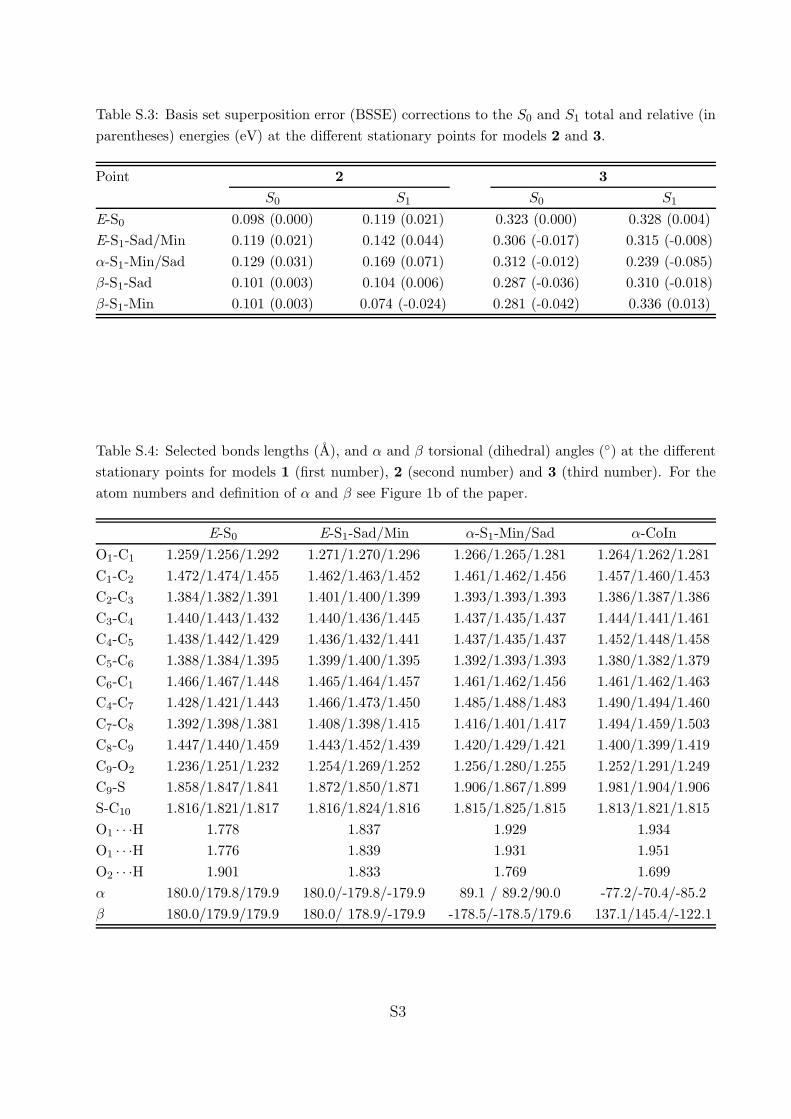
Table S.3: Basis set superposition error (BSSE) corrections to the S0 and S1 total and relative (in

parentheses) energies (eV) at the different stationary points for models 2 and 3.

Point 2 3

S0 S1 S0 S1

E-S0 0.098 (0.000) 0.119 (0.021) 0.323 (0.000) 0.328 (0.004)

E-S1-Sad/Min 0.119 (0.021) 0.142 (0.044) 0.306 (-0.017) 0.315 (-0.008)

α-S1-Min/Sad 0.129 (0.031) 0.169 (0.071) 0.312 (-0.012) 0.239 (-0.085)

β-S1-Sad 0.101 (0.003) 0.104 (0.006) 0.287 (-0.036) 0.310 (-0.018)

β-S1-Min 0.101 (0.003) 0.074 (-0.024) 0.281 (-0.042) 0.336 (0.013)

Table S.4: Selected bonds lengths (A), and α and β torsional (dihedral) angles (◦) at the different

stationary points for models 1 (first number), 2 (second number) and 3 (third number). For the

atom numbers and definition of α and β see Figure 1b of the paper.

E-S0 E-S1-Sad/Min α-S1-Min/Sad α-CoIn

O1-C1 1.259/1.256/1.292 1.271/1.270/1.296 1.266/1.265/1.281 1.264/1.262/1.281

C1-C2 1.472/1.474/1.455 1.462/1.463/1.452 1.461/1.462/1.456 1.457/1.460/1.453

C2-C3 1.384/1.382/1.391 1.401/1.400/1.399 1.393/1.393/1.393 1.386/1.387/1.386

C3-C4 1.440/1.443/1.432 1.440/1.436/1.445 1.437/1.435/1.437 1.444/1.441/1.461

C4-C5 1.438/1.442/1.429 1.436/1.432/1.441 1.437/1.435/1.437 1.452/1.448/1.458

C5-C6 1.388/1.384/1.395 1.399/1.400/1.395 1.392/1.393/1.393 1.380/1.382/1.379

C6-C1 1.466/1.467/1.448 1.465/1.464/1.457 1.461/1.462/1.456 1.461/1.462/1.463

C4-C7 1.428/1.421/1.443 1.466/1.473/1.450 1.485/1.488/1.483 1.490/1.494/1.460

C7-C8 1.392/1.398/1.381 1.408/1.398/1.415 1.416/1.401/1.417 1.494/1.459/1.503

C8-C9 1.447/1.440/1.459 1.443/1.452/1.439 1.420/1.429/1.421 1.400/1.399/1.419

C9-O2 1.236/1.251/1.232 1.254/1.269/1.252 1.256/1.280/1.255 1.252/1.291/1.249

C9-S 1.858/1.847/1.841 1.872/1.850/1.871 1.906/1.867/1.899 1.981/1.904/1.906

S-C10 1.816/1.821/1.817 1.816/1.824/1.816 1.815/1.825/1.815 1.813/1.821/1.815

O1 · · ·H 1.778 1.837 1.929 1.934

O1 · · ·H 1.776 1.839 1.931 1.951

O2 · · ·H 1.901 1.833 1.769 1.699

α 180.0/179.8/179.9 180.0/-179.8/-179.9 89.1 / 89.2/90.0 -77.2/-70.4/-85.2

β 180.0/179.9/179.9 180.0/ 178.9/-179.9 -178.5/-178.5/179.6 137.1/145.4/-122.1

S3

Table S.4: Continuation

β-S1-Sad β-S1-Min β-CoIn Z-S0

O1-C1 1.264/1.265/1.288 1.271/1.271/1.301 1.277/1.276/1.311 1.258/1.257/1.290

C1-C2 1.467/1.467/1.457 1.462/1.462/1.450 1.457/1.457/1.445 1.469/1.470/1.453

C2-C3 1.392/1.391/1.391 1.393/1.393/1.394 1.400/1.399/1.399 1.384/1.383/1.391

C3-C4 1.452/1.451/1.454 1.447/1.447/1.447 1.441/1.441/1.445 1.446/1.448/1.436

C4-C5 1.448/1.448/1.450 1.444/1.444/1.445 1.439/1.439/1.441 1.445/1.448/1.436

C5-C6 1.389/1.390/1.389 1.393/1.393/1.394 1.399/1.398/1.399 1.384/1.383/1.391

C6-C1 1.471/1.469/1.461 1.462/1.462/1.449 1.458/1.458/1.444 1.468/1.469/1.450

C4-C7 1.424/1.423/1.416 1.421/1.421/1.416 1.447/1.443/1.424 1.425/1.421/1.441

C7-C8 1.471/1.472/1.473 1.470/1.470/1.472 1.471/1.473/1.470 1.406/1.412/1.394

C8-C9 1.482/1.436/1.427 1.460/1.461/1.462 1.496/1.498/1.483 1.443/1.435/1.456

C9-O2 1.245/1.254/1.247 1.234/1.228/1.229 1.217/1.223/1.221 1.237/1.247/1.232

C9-S 1.886/1.851/1.885 1.834/1.848/1.839 1.822/1.808/1.827 1.874/1.857/1.854

S-C10 1.816/1.820/1.816 1.820/1.818/1.818 1.820/1.823/1.819 1.816/1.818/1.816

O1 · · ·H 1.827 1.762 1.721 1.790

O1 · · ·H 1.829 1.760 1.719 1.783

O2 · · ·H 1.872 1.967 2.033 1.929

α -173.0/-171.8/-176.2 176.6/ 177.5/177.7 158.8/161.5/174.6 180.0/179.7/-179.7

β 128.9/ 122.7/ 133.8 91.6/ 90.1/ 90.6 102.5/101.2/ 88.4 0.6/ 0.8/ 0.1

S4

Table S.5: Net atomic charges (charges at the adjacent hydrogens are included) in the S0 and

S1 states at the different stationary points for models 1 (first number), 2 (second number) and 3

(third number). For the atom numbers see Figure 1b of the paper.

E-S0 E-S1-Sad/Min

S0 S1 S0 S1

O1 -0.44/-0.42/-0.61 -0.42/-0.42/-0.51 -0.46/-0.42/-0.59 -0.42/-0.42/-0.51

C1 0.19/ 0.19/ 0.22 0.16/ 0.16/ 0.21 0.19/ 0.19/ 0.21 0.16/ 0.16/ 0.20

C2 -0.10/-0.09/-0.09 -0.07/-0.07/-0.03 -0.09/-0.09/-0.08 -0.07/-0.07/-0.04

C3 0.00/ 0.01/ 0.00 -0.04/-0.04/-0.01 -0.00/ 0.01/ 0.01 -0.03/-0.04/-0.01

C4 -0.22/-0.21/-0.21 -0.06/-0.07/-0.05 -0.22/-0.21/-0.21 -0.06/-0.07/-0.06

C5 0.02/ 0.03/ 0.02 -0.01/-0.01/ 0.01 0.02/ 0.03/ 0.02 -0.01/-0.01/ 0.01

C6 -0.13/-0.12/-0.11 -0.05/-0.05/-0.01 -0.12/-0.12/-0.10 -0.04/-0.05/-0.01

C7 0.15/ 0.16/ 0.17 0.04/ 0.05/ 0.03 0.14/ 0.16/ 0.15 0.02/ 0.05/ 0.03

C8 -0.19/-0.19/-0.14 -0.14/-0.09/-0.19 -0.16/-0.19/-0.12 -0.13/-0.09/-0.16

C9 0.19/ 0.18/ 0.19 0.10/ 0.09/ 0.10 0.18/ 0.18/ 0.19 0.10/ 0.09/ 0.10

O2 -0.37/-0.43/-0.34 -0.41/-0.46/-0.41 -0.38/-0.43/-0.36 -0.43/-0.46/-0.43

S -0.14/-0.13/-0.12 -0.14/-0.13/-0.13 -0.13/-0.13/-0.13 -0.14/-0.13/-0.13

C10 0.04/ 0.03/ 0.05 0.04/ 0.03/ 0.05 0.04/ 0.03/ 0.05 0.04/ 0.03/ 0.04

Table S.5: Continuation

α-S1-Min/Sad β-S1-Min

S0 S1 S0 S1

O1 -0.52/-0.51/-0.62 -0.32/-0.32/-0.41 -0.36/-0.36/-0.49 -0.47/-0.47/-0.62

C1 0.16/ 0.16/ 0.17 0.17/ 0.17/ 0.21 0.22/ 0.21/ 0.27 0.14/ 0.14/ 0.17

C2 -0.15/-0.14/-0.13 -0.01/-0.01/-0.00 -0.05/-0.05/-0.04 -0.10/-0.10/-0.08

C3 -0.01/-0.01/ 0.00 0.04/ 0.04/ 0.06 0.10/ 0.09/ 0.12 -0.03/-0.04/-0.02

C4 -0.34/-0.34/-0.32 0.02/ 0.02/ 0.03 -0.13/-0.13/-0.14 -0.16/-0.16/-0.15

C5 -0.01/-0.01/ 0.00 0.04/ 0.04/ 0.06 0.05/ 0.05/ 0.07 -0.04/-0.03/-0.02

C6 -0.15/-0.15/-0.13 -0.01/-0.01/ 0.00 -0.05/-0.05/-0.04 -0.11/-0.11/-0.09

C7 0.21/ 0.23/ 0.21 -0.21/-0.17/-0.21 0.25/ 0.25/ 0.28 -0.14/-0.14/-0.08

C8 0.02/ 0.02/ 0.03 -0.19/-0.14/-0.19 -0.55/-0.52/-0.54 0.11/ 0.12/ 0.12

C9 0.22/ 0.23/ 0.22 0.06/ 0.03/ 0.07 0.12/ 0.13/ 0.12 0.19/ 0.22/ 0.19

O2 -0.32/-0.36/-0.32 -0.47/-0.53/-0.46 -0.46/-0.51/-0.46 -0.27/-0.32/-0.27

S -0.15/-0.13/-0.14 -0.16/-0.15/-0.16 -0.16/-0.14/-0.15 -0.15/-0.12/-0.13

C10 0.03/ 0.04/ 0.04 0.03/ 0.03/ 0.04 0.03/ 0.02/ 0.04 0.04/ 0.02/ 0.04

S5

Table S.5: Continuation

Z-S0

S0 S1

O1 -0.43/-0.42/-0.59 -0.42/-0.42/-0.51

C1 0.20/ 0.20/ 0.22 0.16/ 0.16/ 0.21

C2 -0.11/-0.10/-0.10 -0.08/-0.07/-0.04

C3 0.06/ 0.06/ 0.05 0.02/ 0.02/ 0.04

C4 -0.27/-0.25/-0.26 -0.12/-0.14/-0.10

C5 0.02/ 0.02/ 0.02 -0.02/-0.01/ 0.00

C6 -0.13/-0.12/-0.12 -0.07/-0.07/-0.03

C7 0.13/ 0.13/ 0.15 0.03/ 0.04/ 0.01

C8 -0.16/-0.16/-0.11 -0.04/-0.01/-0.09

C9 0.18/ 0.19/ 0.19 0.07/ 0.08/ 0.06

O2 -0.36/-0.44/-0.33 -0.41/-0.48/-0.42

S -0.15/-0.13/-0.13 -0.16/-0.14/-0.14

C10 0.03/ 0.02/ 0.05 0.03/ 0.02/ 0.04

Table S.6: S0 and S1 charge distributions at the different stationary points in terms of the net

charges on the phenolic (first number) and carbonyl (second number) moieties of the chromophore

for models 1, 2 and 3. The charge on the water molecule(s) is not included.

1 2 3

S0 S1 S0 S1 S0 S1

E-S0 -0.69/-0.31 -0.48/-0.52 -0.61/-0.39 -0.50/-0.50 -0.77/-0.18 -0.40/-0.56

E-S1-Sad/Min -0.69/-0.31 -0.46/-0.54 -0.63/-0.36 -0.47/-0.52 -0.75/-0.22 -0.41/-0.55

α-S1-Min/Sad -1.01/0.01 -0.07/-0.93 -1.00/0.02 -0.05/-0.93 -1.01/0.04 -0.06/-0.91

β-S1-Sad -0.41/-0.59 -0.57/-0.43 -0.31/-0.69 -0.62/-0.38 -0.49/-0.48 -0.46/-0.51

β-S1-Min 0.01/-1.01 -0.92/-0.08 0.02/-1.02 -0.91/-0.09 0.03/-0.99 -0.91/-0.05

Z-S0 -0.67/-0.33 -0.52/-0.48 -0.61/-0.39 -0.52/-0.49 -0.77/-0.19 -0.43/-0.53

S6

Table S.7: Number of unpaired electrons at the chromophore atoms in the S0 and S1 states at the

different stationary points for models 1 (first number) 2 (second number) and 3 (third number).

For the atom numbers see Figure 1b of the paper.

E-S0 E-S1-Sad/Min

S0 S1 S0 S1

O1 0.138/0.145/0.090 0.257/0.243/0.261 0.142/0.151/0.098 0.277/0.268/0.254

C1 0.101/0.105/0.082 0.170/0.162/0.197 0.102/0.106/0.085 0.167/0.158/0.187

C2 0.127/0.131/0.120 0.260/0.248/0.276 0.130/0.136/0.121 0.259/0.250/0.262

C3 0.126/0.130/0.126 0.285/0.265/0.307 0.130/0.134/0.129 0.284/0.253/0.311

C4 0.087/0.088/0.095 0.398/0.387/0.395 0.091/0.094/0.097 0.379/0.353/0.400

C5 0.124/0.126/0.123 0.258/0.251/0.267 0.127/0.130/0.126 0.243/0.233/0.257

C6 0.124/0.127/0.117 0.318/0.297/0.325 0.128/0.132/0.121 0.325/0.305/0.317

C7 0.105/0.106/0.113 0.558/0.562/0.518 0.115/0.116/0.121 0.580/0.552/0.566

C8 0.091/0.084/0.109 0.321/0.354/0.288 0.097/0.091/0.112 0.304/0.318/0.300

C9 0.094/0.083/0.101 0.181/0.208/0.169 0.100/0.091/0.104 0.180/0.222/0.167

O2 0.118/0.095/0.128 0.180/0.171/0.175 0.126/0.102/0.134 0.185/0.177/0.182

C10 0.000/0.000/0.000 0.000/0.001/0.000 0.000/0.001/0.000 0.000/0.002/0.000

S 0.005/0.005/0.005 0.016/0.020/0.016 0.005/0.005/0.005 0.015/0.018/0.015

Table S.7: Continuation.

α-S1-Min/Sad α-CoIn

S0 S1 S0 S1

O1 0.117/0.118/0.090 0.379/0.383/0.331 0.120/0.118/0.099 0.375/0.375/0.326

C1 0.087/0.088/0.074 0.165/0.165/0.164 0.088/0.088/0.091 0.164/0.163/0.190

C2 0.115/0.115/0.111 0.306/0.309/0.289 0.119/0.114/0.122 0.270/0.318/0.241

C3 0.114/0.114/0.117 0.186/0.185/0.184 0.121/0.112/0.139 0.183/0.178/0.178

C4 0.098/0.098/0.107 0.402/0.399/0.411 0.108/0.102/0.151 0.398/0.411/0.330

C5 0.115/0.114/0.117 0.186/0.186/0.184 0.114/0.117/0.146 0.174/0.185/0.196

C6 0.115/0.115/0.111 0.305/0.308/0.290 0.114/0.116/0.125 0.315/0.283/0.251

C7 0.170/0.159/0.174 0.586/0.569/0.576 0.406/0.316/0.554 0.674/0.696/0.552

C8 0.142/0.130/0.147 0.188/0.161/0.198 0.325/0.233/0.481 0.204/0.155/0.334

C9 0.120/0.124/0.121 0.188/0.228/0.185 0.140/0.146/0.156 0.137/0.158/0.155

O2 0.156/0.157/0.158 0.190/0.200/0.191 0.201/0.208/0.221 0.162/0.172/0.202

C10 0.000/0.001/0.000 0.000/0.004/0.000 0.001/0.002/0.002 0.001/0.003/0.002

S 0.005/0.004/0.006 0.016/0.015/0.016 0.008/0.004/0.014 0.011/0.007/0.015

S7

Table S.7: Continuation.

β-S1-Sad β-S1-Min

S0 S1 S0 S1

O1 0.164/0.174/0.113 0.213/0.212/0.182 0.208/0.210/0.156 0.236/0.239/0.163

C1 0.112/0.117/0.089 0.141/0.140/0.145 0.135/0.136/0.107 0.145/0.146/0.147

C2 0.142/0.149/0.125 0.195/0.190/0.191 0.173/0.174/0.152 0.180/0.183/0.151

C3 0.139/0.144/0.131 0.223/0.210/0.241 0.164/0.165/0.149 0.183/0.182/0.202

C4 0.102/0.110/0.098 0.294/0.267/0.307 0.152/0.153/0.137 /0.1670.168/0.160

C5 0.137/0.142/0.130 0.211/0.203/0.225 0.165/0.166/0.151 0.182/0.181/0.202

C6 0.141/0.148/0.126 0.225/0.209/0.229 0.178/0.180/0.158 0.171/0.173/0.148

C7 0.146/0.158/0.143 0.638/0.620/0.600 0.239/0.242/0.209 0.490/0.484/0.555

C8 0.095/0.081/0.120 0.489/0.541/0.412 0.037/0.038/0.035 0.787/0.781/0.792

C9 0.085/0.075/0.092 0.152/0.160/0.138 0.059/0.053/0.060 0.155/0.153/0.154

O2 0.113/0.099/0.126 0.204/0.209/0.189 0.086/0.078/0.087 0.253/0.238/0.253

C10 0.000/0.000/0.000 0.001/0.001/0.001 0.000/0.000/0.000 0.000/0.001/0.000

S 0.004/0.004/0.005 0.015/0.018/0.013 0.003/0.003/0.003 0.018/0.021/0.018

Table S.7: Continuation.

β-CoIn Z-S0

S0 S1 S0 S1

O1 0.228/0.224/0.155 0.231/0.236/0.155 0.143/0.148/0.095 0.249/0.242/0.253

C1 0.140/0.139/0.106 0.139/0.141/0.143 0.103/0.106/0.082 0.160/0.154/0.185

C2 0.186/0.183/0.152 0.181/0.183/0.149 0.129/0.133/0.119 0.256/0.247/0.271

C3 0.170/0.168/0.149 0.176/0.177/0.202 0.128/0.131/0.124 0.257/0.243/0.282

C4 0.186/0.177/0.138 0.176/0.176/0.161 0.088/0.091/0.092 0.379/0.363/0.394

C5 0.170/0.169/0.151 0.175/0.176/0.202 0.126/0.129/0.123 0.243/0.233/0.259

C6 0.193/0.190/0.158 0.171/0.173/0.146 0.127/0.131/0.117 0.291/0.277/0.308

C7 0.316/0.298/0.213 0.542/0.527/0.578 0.110/0.114/0.113 0.545/0.542/0.520

C8 0.028/0.020/0.032 0.823/0.840/0.818 0.090/0.089/0.106 0.357/0.389/0.308

C9 0.067/0.069/0.063 0.146/0.139/0.149 0.094/0.081/0.103 0.213/0.244/0.194

O2 0.095/0.096/0.090 0.197/0.166/0.224 0.111/0.082/0.125 0.193/0.174/0.190

C10 0.000/0.000/0.000 0.003/0.004/0.001 0.000/0.000/0.000 0.001/0.001/0.001

S 0.003/0.003/0.003 0.019/0.022/0.019 0.005/0.005/0.005 0.018/0.022/0.018

S8

Table S.8: Total number of unpaired electrons in the S0 and S1 states and their difference (S1–S0)

at the different stationary points for models 1 (first number) 2 (second number) and 3 (third

number).

α-S1-Min/Sad S1-Min/Sad S0-Min β-S1-Sad β-S1-Min

S0 1.4/1.3/1.3 1.3/1.3/1.3 1.2/1.2/1.2/ 1.4/1.4/1.3 1.6/1.6/1.4

S1 3.1/3.1/3.0 3.2/3.1/3.2 3.2/3.2/3.2/ 3.0/3.0/2.9 3.0/3.0/3.0

S1–S0 1.8/1.8/1.7 1.9/1.8/2.0 2.0/2.0/2.0/ 1.6/1.6/1.6 1.4/1.4/1.6

S9

a=179.8

=179.9b

E-S0

a=179.9

=179.9b

a=180.0

=180.0b

a=180.0

=180.0b

a -= 179.8

=178.9b

a -= 179.9

= 179.9b -

E-S -Sad/Min1

a=89.1

= 178.5b -

a=90.0

=179.6b

a=89.2

= 178.5b -

a=100.0

=137.1b

a=98.7

= 122.1b -

a=107.8

=145.4b

a-CoIn

1

a-S -Min/Sad1

2 3

Figure S.1: Geometries of models 1-3 at the different stationary points and CoIns.

S10

a -= 171.8

=122.7b

a=177.5

=90.1b

a=179.7

=0.8b

a=161.5

=101.2b

a -= 173.0

=128.0b

a=176.6

=91.6b

a=158.8

=102.5b

a=180.0

=0.6b

a -= 176.2

=133.8b

a=177.7

=90.6b

a=174.6

=88.4b

a -= 179.7

=0.1b

b-S -Sad1

1 2 3

b-S -Min1

b-CoIn

Z-S0

Figure S.1: Continuation.

S11

x1 x2

Figure S.2: Gradient difference (x1) and derivative coupling (x2) vectors at the β-CoIn in models

1, 2 and 3, from top to bottom, respectively.

S12

80 85 90 95 100 105

b (degree)

65.00

70.00

75.00

85.00

90.00

95.00

HO

OP

(deg

ree)

CoIn

CoIn

2

1

3

Figure S.3: Changes in the β-torsion and hydrogen out-of-plane (HOOP) coordinate along the loop

of radius 0.005 A for models 1 (blue), 2 (green) and 3 (red).

S13

download fileview on ChemRxivSupporting_Information.pdf (8.40 MiB)