Four Essays on the Political Economy of Economic Reform_Claussen_2003
80
Four essays on the political economy of economic reform Carl Andreas Claussen NO. 3 DOCTORAL DISSERTATIONS IN ECONOMICS
-
Upload
fauwaz-abdul-aziz -
Category
Documents
-
view
218 -
download
0
Transcript of Four Essays on the Political Economy of Economic Reform_Claussen_2003

Four essays on the political economy of economic reform
Carl Andreas Claussen
NO. 3DOCTORAL DISSERTATIONS IN ECONOMICS
The series Doctoral Dissertations in Economics is issued by Norges Bank (Central Bank of Norway) and contains doctoral works produced by employees at Norges Bank, primarily as part of the Bank's research activities. The series is available free of charge from: Norges Bank, Subscription Service E-mail: [email protected] Postal address: PO Box 1179 Sentrum N � 0107 Oslo Norway Previous publication of doctoral dissertations from Norges Bank: (Prior to 2002, doctoral dissertations were published in the series Occasional Papers) Ragnar Nymoen: Empirical Modelling of Wage-Price Inflation and Employment
using Norwegian Quarterly Data. (Occasional Papers no. 18, Oslo 1991) Bent Vale: Four essays on Asymmetric Information in Credit Markets.
(Occasional Papers no. 20, Oslo 1992) Birger Vikøren: Interest Rate Differential, Exchange Rate Expectations and
Capital Mobility: Norwegian Evidence. (Occasional Papers no. 21, Oslo 1994) Gunnvald Grønvik: Bankregulering og bankatferd 1975 � 1991. (Occasional
Papers no. 22, Oslo 1994) Ingunn M. Lønning: Controlling Inflation by use of the Interest Rate: The Critical
Role of Fiscal Policy and Government Debt. (Occasional Papers no. 25, Oslo 1997)
Tom Bernhardsen: Interest Rate Differentials, Capital Mobility and Devaluation Expectations: Evidence from European Countries. (Occasional Papers no. 27, Oslo 1998)
Øistein Røisland: Rules and Institutional Arrangements for Monetary Policy. (Occasional Papers no. 29, Oslo 2000)
© Norges Bank 2003 The text may be quoted or referred to, provided that due acknowledgement is given to the author and Norges Bank. Views and conclusions expressed in this dissertation are the responsibility of the author alone. The author may be contacted at: [email protected]
This book was printed and bound at Lobo Media AS, Oslo. The text was written in 10-point Times by the author.
Quaisar Farooq Akram: State Dependent Effects in Labour and Foreign ExchangeMarkets. (Doctoral Dissertations in Economics no. 1, Oslo 2002)
Kai Leitemo: Inflation targeting and monetary policy. (Doctoral Dissertations in Economics No. 2, Oslo 2002)

Four Essays on the Political Economy of
Economic Reform
By
Carl Andreas Claussen
Dissertation for the degree dr. polit. Institute of Economics
Faculty of Social Sciences University of Oslo


3
Contents
Preface 4 Author's preface 5 Chapter 1. Introduction and overview 7 Chapter 2. Persistent inefficient redistribution 13 Chapter 3. Why keep a bad government? 27 Chapter 4. On the dynamic consistency of reform and compensation schemes 41 Chapter 5. The time consistency of two tier labor market reforms 59

DOCTORAL DISSERTATIONS IN ECONOMICS NO. 3 4
Preface
This thesis provides political-economy explanations for the prevalence of inefficient government policies. Possible solutions to the problem of non-adoption of efficient policies are also provided. Understanding why inefficient government policies exist, and how they may be reformed, is key in the field of political economy. A leading example is trade policies, where the reality of most countries’ policies is so blatantly contrary to all the normative prescriptions of the economist that there seems to be no way to understand it except by delving into the politics. Labor market policies provide other examples. The recent wave of economic reforms has heightened the interest in these questions. The thesis is part of Claussen’s Dr. Polit exam at the University of Oslo. Claussen defended the thesis on March 24, 2003. Oslo May 2003 Monetary Policy Department Kristin Gulbransen Director

AUTHOR'S PREFACE 5
Author’s preface
This thesis was written mainly during two periods. In the first period, from November 1996 to February 1998, I was a research fellow at Agder College, financed by a grant from the SIS-program. In the second period, from October 2000 to December 2001, I had a scholarship from Norges Bank, and benefited from the kind hospitality of the Stockholm Institute of Transition Economics at the Stockholm School of Economics, and from the IMF. In 1997 I spent a month at the Humboldt Universität zu Berlin and received financial support from the Ruhrgas-foundation. I am also grateful to Norges Bank for the opportunity to finishing the thesis this year. An author’s debts are a pleasure to mention. First of all, I am grateful to my supervisor Geir B. Asheim. He has always responded quickly to the various drafts submitted, and his comments have always been extremely valuable. Our discussions and his encouragement have been crucial for my work. Thanks also to Victor D. Norman and Terje Lensberg for suggestions and stimulating discussions during my time at Agder College. I have also benefited from discussions and comments from many colleagues, including Karsten Stæhr, Ragnar Torvik, Era-Dabla Norris, Paul R. Wade and Douglas Lundin. Janet Aagenæs, David L. Cameron and Veronica Harrington have provided editorial assistance. Finally, I would like to express my gratitude to Lisa, for her encouragement and for her patience. Oslo September 12, 2002 Carl Andreas Claussen

DOCTORAL DISSERTATIONS IN ECONOMICS NO. 3 6

CH. 1 INTRODUCTION AND OVERWIEV 7
Chapter 1
Introduction and overview
Economists have always been better at telling policymakers what to do than at explaining why policymakers do what they do. Rodrik (1993)
1. Introduction During the last two decades we have seen a wave of economic reforms all over the world. Most striking is perhaps the transformation of the centrally planned economies in Eastern Europe into market economies. But also in other regions there have been significant reforms. What determined the timing and content of these reforms? Why are governments generally so reluctant to undertake reforms? Part of the answer to these and related questions can be found in “pure” economics. The expected outcome from reform might be negative, the uncertainty might be too high, and so forth. However, pure economic explanations often do not carry through. This has spurred the exploding literature on the political economy of economic reform.
Roughly stated, political economy is the analysis of how economics affect politics and how politics affect economics. Drazen (2000, p. 16) explains it the following way.
“Political economy starts with the problem of choice in a society with heterogeneous agents, but with a very different focus than multi-agent welfare economics. The focus is on the process by which it is decided what policy to adopt, and, more specifically, on what policy choice will emerge from a specific political process. The issue is not a technical problem of the implication of different weights, but the political problem of how the weights are chosen (representing the question of how conflicts of interests are resolved) and its economic implications.“

DOCTORAL DISSERTATIONS IN ECONOMICS NO. 3 8
The literature on the political economy of reform utilizes this type of analysis to explain the reform process and the non-adoption of reform.1
This thesis consists of four essays on the political economy of economic reform. The essays cover various aspects of the political economy of reform but are linked in several ways. The aim of this introductory chapter is to give a brief and non-technical overview of the essays and to explain the links among them. The discussion of the contribution of my research to the existing literature will be taken in each essay separately. 2. Essay 1. Persistent inefficient redistribution
The motivation for the first essay (chapter 2) is to explain the widespread use of economically inefficient means for redistribution. The use of trade barriers offers an example. Trade barriers divert resources to domestic producers, but at the cost of a deadweight loss. Why not simply tax the losers from the barriers and transfer the receipts directly to the domestic producers (assuming that this produces a smaller deadweight loss)?
In the essay I look at representative democracy. The government decides what policy to pursue, but the voters can change the government by selecting opposition politicians through elections. I assume that the politicians including the incumbent politician (the government) knows that economically more efficient means for redistribution than the one currently used exist. Can the incumbent still find it optimal not to reform? The answer is yes if three conditions are fulfilled: (i) The voters must know less about the efficiency of policies than the politicians, and they must believe that the policy pursued is efficient in some states of the world. (ii) The voters must not know the preferences of the different politicians. (iii) “Ideologist” politicians that would make reforms even if it were inefficient must be present. When these conditions are fulfilled, an incumbent that prefers to redistribute to special interests can use the inefficient method to mask the real redistributive aim of policy. If the incumbent use the more efficient method for redistribution, the incumbent reveals that it prefers to redistribute to special interests, and such an incumbent is not re-elected. Consequently, the government prefers to stick with the inefficient form of redistribution.
An evident question is why rational voters stay ignorant about the efficiency of the policy. Why do the opposition politicians not provide the voters with information regarding the inefficiency of the policy pursued? In the model in the essay the reason is that all politicians have incentives to pretend to be good. Thus the information content of their claims is rendered worthless for the voters.
1 Drazen (2000) has recently surveyed this literature. Useful earlier surveys are Rodrik (1993, 1996) and Tommasi and Velasco (1996).
CH. 1 INTRODUCTION AND OVERWIEV 9
3. Essay 2. Why re-elect a bad government?
The motivation for the second essay (chapter 3) is to explain re-election of openly corrupt governments and governments openly redistributing to special interests at the expense of the vast majority of the population.
In the essay, I ask if there can be non-adoption of reform even if the voters know which policy is best. I assume a representative democracy where the government decides what policy to pursue, but the voters can change the government by selecting opposition politicians through elections. The incumbent politician (the government) pursues a policy that is contrary to the interest of all voters, and everyone observes this. At the same time there are opposition politicians available for office in every election. Some of these prefer to pursue policies even worse than the policy pursued by the current incumbent, but others prefer to pursue the policies preferred by the voters. Can it still be rational for the voters to re-elect an incumbent pursuing policies contrary to their interest? The answer is yes if the opposition politicians cannot credibly convey information to the voters about which policy they will pursue if in office. The voters will prefer to keep the incumbent if the policy pursued is not considered too detrimental. The reason is that by electing a challenger, the voters run the risk of electing a very poor politician who they have to stick with for some time.
Again evident question is why rational voters stay ignorant about the politicians’ type. Here too, the answer is as in essay 1. Since all politicians have incentives to pretend to be good, the information content of their claims is rendered worthless for the voters.
4. Essay 3. On the dynamic consistency of reform and compensation
schemes
In the third essay (chapter 4) I look for ways to overcome the problem of non-adoption of reform. A natural starting point is to look for ways to compensate the losers from reform. To keep things relatively simple I abstract from the principal-agent problems in the models of the first two essays, and assume that policy is determined by majority decisions.
The essay has the seminal article by Fernandez and Rodrik (1991) as the starting point. The authors show how there is an inherent status quo bias if there is individual-specific uncertainty regarding the gains from reform. I make three main changes to the Fernandez-Rodrik model: I allow for compensation to the losers, introduce an infinite time horizon, assume that the share of losers from reform decreases over time, and assume that in the end all individuals gain from reform. Furthermore I assume that the individuals cannot make binding commitments.
The model captures two major aspects of the dynamics of real world reforms: first, in the short run the losers are strong and able to block or reverse reform. Second, over time and as a result of reform the losers’ influence over policy declines. Some labor market reforms in

DOCTORAL DISSERTATIONS IN ECONOMICS NO. 3 10
Europe, dual track reforms in China and many reforms in the formerly socialist economies of Eastern Europe have these aspects.
I find that to accept reform, losers first demand partial compensation. The compensation demanded declines over time until the last period when the losers have political influence. In that period the compensation increases dramatically. After this compensation there is no compensation to the losers. The pattern of compensation follows from the development of the losers’ political influence and the realization of the aggregate gains during reform. In the initial phase the losers know that they can make demands also during the following periods. They are therefore satisfied with partial compensation. Later, when the reform takes hold, the losers’ ability to demand compensation is lost. Therefore, they demand full compensation for continued reform some time before the reform takes hold.
I also look at the effect of increasing the irreversibility of reform. I find that increasing the economic cost of reversing reform is often a bad idea. It can only be a good idea if the losers are liquidity constrained at the time when the losers have to be paid off completely.
In the model presented in the essay I assume that all losers are compensated. A possible criticism to this assumption is that it is not necessary to compensate all losers to get a majority for reform. However, looking closer at the potential bargaining game between the players over the gains from reform, I find that it is cheaper for the winners from reform to compensate all losers than to compensate any smaller share of the losers.
5. Essay 4. The time consistency of two-tier labor market reforms
Also in the fourth essay (chapter 5), I look for ways to overcome the problem of non-adoption of reform through compensation to the losers. As in the third essay, I keep things simple by abstracting from principal-agent problems, and assume that policy is determined by majority decisions.
I look at a concrete real-world reform that creates a dynamic situation similar to the one described by the more abstract model in essay 3. The reform is a two-tier reform on the labour market. Two-tier reforms are reforms where the cost of firing workers is reduced for new labour contracts, while for contracts entered before reform, firing costs remain unchanged. Two-tier reforms have been quite common in Europe over the last few decades. The two-tier mechanism compensates the losers from reform implicitly, but gradually changes the political constellations as described in the third essay.
Previous research has found that a time consistency problem limits the scope for two-tier labor market reforms since the winners prefer to pursue full reform and eliminate the implicit compensations as soon as they are politically strong enough to make such decisions. My hypothesis, which is supported in the essay, is that this conclusion hinges on an implicit assumption of fiscal illusion. If the voters know that there is a link between unemployment

CH. 1 INTRODUCTION AND OVERWIEV 11
levels and taxes, they also know that higher unemployment requires higher taxes. Since a two-tier reform gives lower unemployment during transition, taxes are smaller under a two-tier reform than under a full reform. Consequently, all voters prefer continuation of two-tier reform to a complete reform and the time consistency problem disappears.
6. Links between the essays
In general, the essays of the thesis are linked thematically on the basis of economic reform. There are also closer thematical links between the first and the second, and between the third and the forth. The second essay is a natural follow up of the first, in that there are two sorts of asymmetric information in the first essay whereas there is only one of these in the latter. The third and fourth essays are linked as both look at compensation schemes under reforms where the political power of the losers from reform is shrinking following a Markov process. In fact, the model in the fourth essay is a real world application of the third.
Furthermore, the models in all four essays are political economy models, all models are dynamic, and each has an infinite time horizon. The equilibria are dynamically consistent. That is, the agents’ expectations are formed as part of the equilibrium, and are consistent with the equilibrium and equilibrium behavior at any point in time.
References Drazen, A. (2000), Political Economy in Macroeconomics, Princeton University Press. Fernandez, R. and D. Rodrik (1991), “Resistance to reform: Status quo bias in the presence of
individual-specific uncertainty,” American Economic Review, vol. 81, no. 5. Rodrik, D. (1993), “The positive economics of policy reform,” American Economic Review,
vol. 83, no. 2. Rodrik, D. (1996), “Understanding economic policy reform,” Journal of Economic Literature,
vol. 34, no. 1. Tommasi, M and Velasco, A. (1996), “Where are we in the political economy of reform?”
Policy Reform, vol. 1, no. 2.

DOCTORAL DISSERTATIONS IN ECONOMICS NO. 3 12
CH. 2 PERSISTENT INEFFICIENT REDISTRIBUTION 13
Chapter 2
Persistent inefficient redistribution *
Carl Andreas Claussen**
Norges Bank
Abstract
Why do governments redistribute through indirect and inefficient means? An intuitive hypothesis is that it masks the real aim and cost of policy. In this paper we construct a dynamic model with an infinite horizon, political competition, rational individuals and asymmetric information regarding the efficiency of policy and politicians’ preferences to test this hypothesis. While the previous (formal) literature explains one-time projects like the building of a dam, bridge or an airport, we are able to explain the persistent use of inefficient means like regulation and subsidies for redistributive purposes. Keywords: Political economy, Inefficient redistribution, Reform, Special interests. JEL codes: D72, C73.
* Thanks to Geir Asheim for guidance. Much of this work was done when I was visiting SITE at the Stockholm School of Economics. Their hospitality is gratefully acknowledged. Thanks also to Norges Bank for financial support. Remaining omissions and mistakes are mine. The views presented are mine and do not necessarily represent those of Norges Bank. ** [email protected]. Norges Bank, box 1179 Sentrum, 0107 Oslo, Norway.

DOCTORAL DISSERTATIONS IN ECONOMICS NO. 3 14
1. Introduction Governments redistribute. Much of this is rather direct and explicit, but large parts are indirect, implicit, and has large deadweight losses (see e.g. Tullock (1983)). Often more efficient redistributive means exist. Why not use the most efficient means? This question is the focus of the current paper.
An intuitively appealing answer is that indirect means are used to mask the real aim and cost of policies. Aims are masked by transfer mechanisms justifiable on grounds other than redistribution, so-called disguised transfer mechanisms (Tullock 1983).1 The costs are masked by the mechanisms with concealed costs (Coate and Morris 1995). Import quotas and different kinds of regulations are examples of policies with concealed costs. Answers based on these arguments are often associated with the Virginia school of political economy, and are sometimes denoted “the Virginia View” (see e.g. Coate and Morris (1995)).
Coate and Morris (1995) provide a principal formal test of the Virginia view. They find that the Virginia view holds if there is asymmetric information regarding both the efficiency of policy and the preferences of the politicians. They pursue their test on a common agency two-period model of political competition where the voters are rational but imperfectly informed. The disguised transfer mechanism is a one-time project like the building of an airport or a bridge etc., where the cost of the project is common knowledge. The project is undertaken in the first period, and the outcome is observed in the second period before the voters decide whether to re-elect the incumbent. If the incumbent in the first period explicitly redistributes, she signals that she is “bad”, and is replaced by a challenger. If she uses the disguised mechanism, the voters cannot say whether she is “good” or “bad” since the state of the world is unknown to them. In equilibrium the project is undertaken in the first period even if the state of the world is such that the project is inefficient in expected terms.
Although one-time projects are important redistributive tools, the widespread use of apparently inefficient subsidies, regulations, tariffs etc. suggests that permanent policies are more important. In this paper we test formally whether the Virginia view holds for more permanent inefficient policy measures. For this purpose, we construct a model where policies can persist and produce inefficient results for an infinite number of periods. We assume that the voters cannot observe the outcome of the policy perfectly, but the policy is inefficient in expected terms. The model has an infinite horizon, political competition and rational voters. The main characteristics of the Coate and Morris model are maintained: some politicians prefer to redistribute and others not, redistribution can take place directly or through a public policy, there are elections where the incumbents can be replaced by a political challenger, and
1 The idea is that a policy is efficient only in some states of the world, but the state of the world is not known to the voters (Rodrik 1995).

CH. 2 PERSISTENT INEFFICIENT REDISTRIBUTION 15
there is some “initial” asymmetric information both regarding the efficiency of policy and the preferences of the politicians.
Our finding is that the Virginia view holds and that it explains permanent inefficient redistribution. As in the Coate and Morris model, asymmetric information both regarding the efficiency of policy and the preferences of the politicians is assumed to obtain the result. In equilibrium the incumbent never uses the most efficient means for redistribution because that would reveal that she is redistributive and that the policy is pursued for redistributive reasons, not for efficiency reasons. The voters do not change the incumbent for a challenger even though the “initial“ expected gain from doing this is positive. The reason is that after observing the incumbent’s policy, their measure of the likelihood that it is efficient has increased. In addition to the asymmetric information regarding the efficiency of the policies and the preferences of the politicians, but differently from the Coate and Morris framework, we need "ideologist" politicians that always reform. If there is no “ideologist”, the citizen can costlessly try out the different challengers since the challengers will either pursue the same or a better policy.
The current paper comes under at least two branches of the modern literature on political economy. One is the literature on the form of transfers to special interests. Coate and Morris (1995) and Acemoglu and Robinson (2001) provide an overview of some of this discussion. Another branch is the literature on the political economy of economic reform. Drazen (2000), Rodrik (1996) and Tommasi and Velasco (1996) survey this literature.
Several authors have elaborated on the Coate and Morris two-period model (see e.g. Bordignon and Minelli 2001 and Brett and Keen 2000). We are not aware of any attempts to test the Virginia view in a multiperiod setting with rational individuals and political competition.
The paper is organized as follows: We present the model in section 2, and find equilibrium in section 3. In section 4 we briefly discuss some of our assumptions and conclude.
2. Model
We look at an economy populated with N identical individuals who consume and vote. Out of these N individuals, n< ½N have successfully managed to overcome free-rider problems and formed a special interest group. We denote this sub-group S.
The only political issues concern whether there should be redistribution from the general public to the special interest, and which of two forms this redistribution should take. The incumbent politician has three policy options available:
(i) No intervention in the economy (no redistribution).
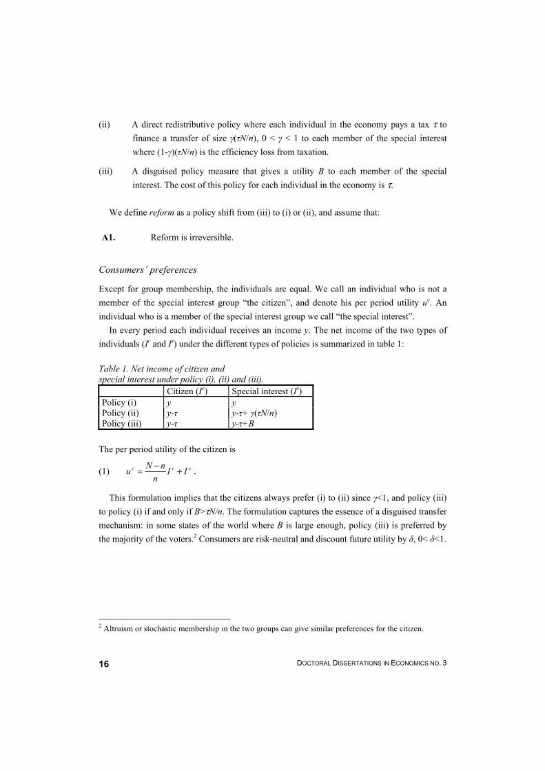
DOCTORAL DISSERTATIONS IN ECONOMICS NO. 3 16
(ii) A direct redistributive policy where each individual in the economy pays a tax τ to finance a transfer of size γ(τN/n), 0 < γ < 1 to each member of the special interest where (1-γ)(τN/n) is the efficiency loss from taxation.
(iii) A disguised policy measure that gives a utility B to each member of the special interest. The cost of this policy for each individual in the economy is τ.
We define reform as a policy shift from (iii) to (i) or (ii), and assume that:
A1. Reform is irreversible.
Consumers’ preferences
Except for group membership, the individuals are equal. We call an individual who is not a member of the special interest group “the citizen”, and denote his per period utility uc. An individual who is a member of the special interest group we call “the special interest”.
In every period each individual receives an income y. The net income of the two types of individuals (Ic and Is) under the different types of policies is summarized in table 1: Table 1. Net income of citizen and special interest under policy (i), (ii) and (iii). Citizen (Ic) Special interest (Is) Policy (i) y y Policy (ii) y-τ y-τ+ γ(τN/n) Policy (iii) y-τ y-τ+B
The per period utility of the citizen is
(1) scc IIn
nNu +−= .
This formulation implies that the citizens always prefer (i) to (ii) since γ<1, and policy (iii) to policy (i) if and only if B>τN/n. The formulation captures the essence of a disguised transfer mechanism: in some states of the world where B is large enough, policy (iii) is preferred by the majority of the voters.2 Consumers are risk-neutral and discount future utility by δ, 0< δ<1.
2 Altruism or stochastic membership in the two groups can give similar preferences for the citizen.

CH. 2 PERSISTENT INEFFICIENT REDISTRIBUTION 17
Politicians
Politicians are risk-neutral and have the same discount factor as the citizens. They can be of three different types:
Benevolent politicians maximize the expected utility of the citizen.
(2) ck
t
kBt EuV ∑
∞
= δ .
Redistributive politicians always prefer redistribution to S to no redistribution. They behave as if they maximize the following3
(3) ( )sk
ck
t
kRt IIEV +=∑
∞
αδ .
Here ( ) nnN /0 −<≤α measures the degree of benevolence of the redistributive politicians. The benevolence parameter is the same for all redistributive politicians, but the closer α is to (N-n)/n, the more benevolent the redistributive politicians are. Ideologist politicians always prefer policy (i).
(4) cIt IV =
We assume that the politicians derive utility from the policies pursued whether in office or not. This means that they have no additional utility from being in power. A2. Politicians’ utility both in and out of office is given by (2), (3) or (4).
Timing of events
At the beginning of every period the incumbent politician sets policy and all players observe the policy and its outcome. By the end of the period there is an election where the majority (the citizen) either re-elect the incumbent or elect the challenger.
In period t=0 nature chooses the realisation of B (that stays the same for all future periods) and an incumbent. In the following periods the incumbent at the beginning of the period is the one that was elected at the end of the preceding period. The number of periods is infinite.
3 In the appendix to chapter 3 I show how (3) follows from a government maximizing a weighted sum of contributions (bribes) from the special interest and the welfare of the general public. A more direct interpretation is that politicians have direct preferences for his home district, farmers, etc.

DOCTORAL DISSERTATIONS IN ECONOMICS NO. 3 18
Information structure
There are two types of information asymmetries in the model. The first relates to the politicians’ types and the other regards the efficiency of reform, i.e. the realization of B.
It is common knowledge that nature draws the incumbent and the challengers according to a probability distribution λ=(λR, λB, λI), where the first term is the probability that the politician is redistributive, the second is the probability that the politician is benevolent and the last term is the probability that the politician is an ideologist.4 However,
A3. only the politicians themselves know their own type.
Similarly, it is common knowledge that the variable B can take one of two values, BL or
BH, but, A4. the politicians know the realization of B, whereas the citizens only know that the
probability that B=BH is π.
The parameters of the model, the functional forms and the timing of events are common
knowledge. Restricting the model
To tailor the model to a situation we want to describe, we have to place some more restrictions on the model. The first restriction states that for the citizen, policy (ii) is preferred to (iii) in expected terms
R1. nNBB LH γτππ <−+ )1( .
This means that the prior perceptions of the voters (the citizen) are such that they would actually vote for (ii) to (iii) if there was direct voting on the issue.
The second restriction ensures that there exists an equilibrium in which it is optimal to keep the incumbent politician if she plays (iii).
R2. ( ) ( )( ) ( ) τ
πλλπλλπλλπλλ
nNBB
RRII
LRRHII ≥−−+−−−+−
)1(11)1(11 .
4 λ corresponds to what Coate and Morris (1995) call the challengers’ initial reputation.

CH. 2 PERSISTENT INEFFICIENT REDISTRIBUTION 19
The two restrictions imply λI(1- λI)> λR(1- λR) and
(5) BH > τN/n > γ(τN/n) >BL,
which in turn implies that policy (iii) is efficient if and only if B=BH.
The third restriction ensures that the redistributive politician prefers policy (iii) to (i) even if B=BL, R3. ( )τα+> 1LB .
Together with (5), R3 also implies that a redistributive incumbent prefers (ii) to (i). The game and equilibrium concept
The model defines a multistage game with an infinite horizon between the incumbent politician, the challengers and the citizen. There is incomplete information and the players move sequentially within each stage.
Before the first stage of the game nature chooses the realization of B for the whole game, and the incumbent’s type for stage 1. In each stage of the game the incumbent first chooses actions from (i)-(iii) if there has been no reform and (i) and (ii) if there has been a reform. Then the challengers make claims regarding the efficiency of reform (π) and their type. Then the citizen either re-elects the incumbent or picks a challenger. In the latter case, nature chooses the type of the new incumbent for the next stage.
The information structure of the game is such that the incumbent knows her own type and the realization of B. The citizen knows that the probability that B=BH is π, and the probability that the incumbent is of the different types is given by the vector λ. Both the incumbent and the citizen know that the probability that the challengers are of the different types is given by the vector λ.
Each stage seen in isolation is a Bayesian extensive game with observable actions. There are links between each stage. Extracted information regarding the efficiency of the reform and the incumbent’s type is carried over from one stage to the next.
Bayesian equilibrium is the natural equilibrium concept for the game. This equilibrium consists of a strategy and beliefs for each player that satisfy two properties. First, each player’s beliefs are consistent with all players’ strategies in the sense that they are generated by Bayesian updating where possible. Second, each player’s strategy is optimal given these beliefs and the strategies of the other players.

DOCTORAL DISSERTATIONS IN ECONOMICS NO. 3 20
3. Solving the model
In the game described in section 2, claims made by the challenger have no direct impact on the players’ payoffs. Thus, challengers’ campaign statements regarding type or program (or anything else) are “cheap talk”. In games with cheap talk there are always “babbling” equilibria where the receiver ignores the sender’s signals. In our setting this implies that there are equilibria where the citizen ignores the political challengers’ claims. These are equilibria where the challengers play no active role in the game, and where the game can be considered a game between the citizen and the incumbent only. We will concentrate on such equilibria. Here the citizen and the incumbent always believe the probability that each of the challengers is of the different types is given by λ.
If there has been a reform, the only political issue is whether there should be redistribution or not. On this issue, both benevolent and ideologist incumbents have interests coincident with the citizen and such incumbents will play (i). Thus, the citizen has no incentives to change such incumbents for a challenger. Furthermore, since politicians always have utility from the policies pursued (and not only if in office (c.f. A2)), there is a net gain for the redistributive incumbents from playing (ii) even if that means that they are not re-elected. Lemma 1 gives the equilibrium strategies for the players if there has been a reform. This equilibrium is supported by off equilibrium path beliefs that are such that if the citizen observes the incumbent playing (ii) after having played (i) at an earlier stage, then he believes the incumbent is redistributive. The proof is straightforward.
Lemma 1 If A1 - A3, R1 - R3, and there has been a reform, then the equilibrium strategies are:
Citizen: Elect a challenger if and only if incumbent played (ii).
Incumbent: If ideologist or benevolent, always play (i). Play (ii) if
redistributive.
It follows directly from lemma 1 that ideologist incumbents will find it optimal to play (i)
also if there has been no reform. The same is the case if the incumbent is benevolent and reform is efficient. But we want to prove the existence of an equilibrium where the citizen re-elects incumbents playing (iii), and where an incumbent plays (iii) even if reform is efficient. A combination of strategies where this is the case is the following: the citizen elects a challenger if and only if the incumbent plays (ii). The incumbent always plays (i) if she is ideologist, always plays (iii) ((ii)) if she is redistributive and there has been no reform (been reform), and plays (iii) ((i)) if benevolent and B=BH (B=BL).
CH. 2 PERSISTENT INEFFICIENT REDISTRIBUTION 21
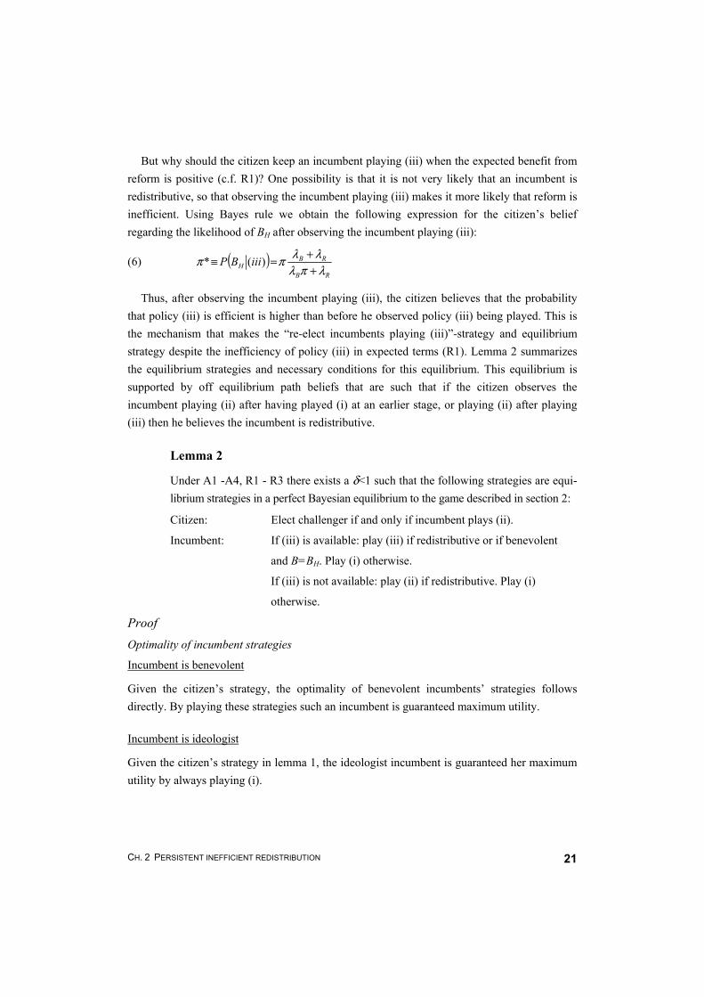
But why should the citizen keep an incumbent playing (iii) when the expected benefit from reform is positive (c.f. R1)? One possibility is that it is not very likely that an incumbent is redistributive, so that observing the incumbent playing (iii) makes it more likely that reform is inefficient. Using Bayes rule we obtain the following expression for the citizen’s belief regarding the likelihood of BH after observing the incumbent playing (iii):
(6) ( )RB
RBH iiiBP
λπλλλππ
++=≡ )(*
Thus, after observing the incumbent playing (iii), the citizen believes that the probability that policy (iii) is efficient is higher than before he observed policy (iii) being played. This is the mechanism that makes the “re-elect incumbents playing (iii)”-strategy and equilibrium strategy despite the inefficiency of policy (iii) in expected terms (R1). Lemma 2 summarizes the equilibrium strategies and necessary conditions for this equilibrium. This equilibrium is supported by off equilibrium path beliefs that are such that if the citizen observes the incumbent playing (ii) after having played (i) at an earlier stage, or playing (ii) after playing (iii) then he believes the incumbent is redistributive.
Lemma 2
Under A1 -A4, R1 - R3 there exists a δ<1 such that the following strategies are equi-librium strategies in a perfect Bayesian equilibrium to the game described in section 2:
Citizen: Elect challenger if and only if incumbent plays (ii).
Incumbent: If (iii) is available: play (iii) if redistributive or if benevolent
and B=BH. Play (i) otherwise.
If (iii) is not available: play (ii) if redistributive. Play (i)
otherwise.
Proof Optimality of incumbent strategies
Incumbent is benevolent
Given the citizen’s strategy, the optimality of benevolent incumbents’ strategies follows directly. By playing these strategies such an incumbent is guaranteed maximum utility. Incumbent is ideologist
Given the citizen’s strategy in lemma 1, the ideologist incumbent is guaranteed her maximum utility by always playing (i).
DOCTORAL DISSERTATIONS IN ECONOMICS NO. 3 22
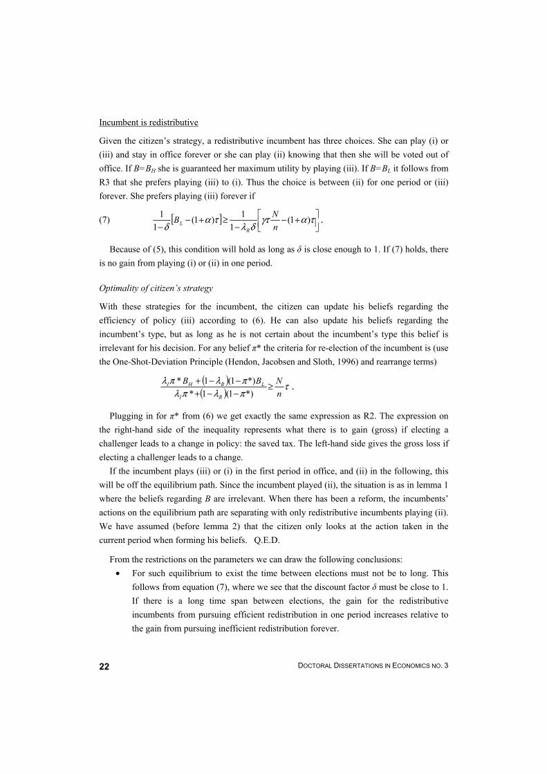
Incumbent is redistributive
Given the citizen’s strategy, a redistributive incumbent has three choices. She can play (i) or (iii) and stay in office forever or she can play (ii) knowing that then she will be voted out of office. If B=BH she is guaranteed her maximum utility by playing (iii). If B=BL it follows from R3 that she prefers playing (iii) to (i). Thus the choice is between (ii) for one period or (iii) forever. She prefers playing (iii) forever if
(7) [ ]
+−
−≥+−
−ταγτ
δλτα
δ)1(
11)1(
11
nNB
RL .
Because of (5), this condition will hold as long as δ is close enough to 1. If (7) holds, there is no gain from playing (i) or (ii) in one period. Optimality of citizen’s strategy
With these strategies for the incumbent, the citizen can update his beliefs regarding the efficiency of policy (iii) according to (6). He can also update his beliefs regarding the incumbent’s type, but as long as he is not certain about the incumbent’s type this belief is irrelevant for his decision. For any belief π* the criteria for re-election of the incumbent is (use the One-Shot-Deviation Principle (Hendon, Jacobsen and Sloth, 1996) and rearrange terms)
( )( ) τ
πλπλπλπλ
nNBB
RI
LRHI ≥−−+−−+
*)1(1**)1(1* .
Plugging in for π* from (6) we get exactly the same expression as R2. The expression on the right-hand side of the inequality represents what there is to gain (gross) if electing a challenger leads to a change in policy: the saved tax. The left-hand side gives the gross loss if electing a challenger leads to a change.
If the incumbent plays (iii) or (i) in the first period in office, and (ii) in the following, this will be off the equilibrium path. Since the incumbent played (ii), the situation is as in lemma 1 where the beliefs regarding B are irrelevant. When there has been a reform, the incumbents’ actions on the equilibrium path are separating with only redistributive incumbents playing (ii). We have assumed (before lemma 2) that the citizen only looks at the action taken in the current period when forming his beliefs. Q.E.D.
From the restrictions on the parameters we can draw the following conclusions: • For such equilibrium to exist the time between elections must not be to long. This
follows from equation (7), where we see that the discount factor δ must be close to 1. If there is a long time span between elections, the gain for the redistributive incumbents from pursuing efficient redistribution in one period increases relative to the gain from pursuing inefficient redistribution forever.

CH. 2 PERSISTENT INEFFICIENT REDISTRIBUTION 23
• It follows from R1 and R2 that λI(1- λI)> λR(1- λR) is a requirement for an equilibrium with inefficient redistribution to exist. Thus, the share of benevolent politicians does not matter as long as it is larger than zero. If the share of ideologists and redistributive politicians are each less than ½ of all politicians, it is sufficient that the share of ideologists is larger than the share of redistributive politicians.
The appendix includes a numerical example where restriction R1 - R3 and condition (7) hold simultaneously. We can now state our proposition.
Proposition
Under A1 - A4 and R1 - R3, and if elections are sufficiently frequent, there exist perfect Bayesian equilibrium outcome to the game described in section 2 where policy (iii) is persistently pursued when B=BL.
Proof
If B=BL and the incumbent in period t=0 is redistributive, then it follows from lemma 2 that the perfect Bayesian equilibrium outcome to the game described in section 2 is that policy (iii) is pursued forever. The appendix gives a configuration of parameter values for which all the restrictions and conditions for lemma 1 hold simultaneously. Q.E.D.
Proposition 1 states that the Virginia View holds in our model; i.e. there exist equilibria where the government prefers to pursue (iii), and where the voters prefer to keep a redistributive incumbent playing (iii) even though
• policy (iii) is not efficient in expected terms (reform is efficient in expected terms),
• policy (iii) is in fact inefficient (B=BL), and
• there are more efficient means for redistribution available.
The reason why the incumbent does not use the more efficient means for redistribution is as the Virginia view prescribes: by using the most efficient means for redistribution the incumbent will reveal that she is redistributive and that policy (iii) is pursued for redistributive reasons, not for efficiency reasons. The reason why the citizen does not elect a challenger even if the expected gain from reform is positive is twofold. First, since he observes that the incumbent does not reform, he becomes more confident that reform is inefficient. Second, there is a risk that the challenger will reform even though that is not efficient. If this risk did not exist, the citizen could simply try out challengers to see if anyone reforms. This would be risk-free since the challengers will either pursue the same or a better policy.

DOCTORAL DISSERTATIONS IN ECONOMICS NO. 3 24
4. Discussion and concluding remarks
The aim of this paper has been to explain the persistent use of apparently inefficient means for redistribution. Concretely, we test the Virginia view that suggests that inefficient means are used to conceal the real redistributive aim and the real cost of policy.
As in the previous formal literature, we construct a model with initial asymmetric information regarding both the efficiency of policy and the preferences of the politicians. In contrast to previous literature, we introduce an infinite horizon and allow for opposition politicians to play an active role since they can provide the voters with information regarding the efficiency of policy and their own preferences.
We show that also under these circumstances the Virginia view holds. Additionally, our model explains the persistent use of inefficient means, and not only one-time projects like the building of an airport, a bridge etc.
There are two simple mechanisms that prevent voters from throwing the incumbent out of office even though the expected efficiency of the policy pursued is negative initially: the first is that there is a risk of electing a politician who is worse than the current one. This (worse) politician is an ideologist who reforms even if that is not efficient. Without this ideologist, the Virginia view does not hold in our setting with an infinite horizon. The second reason why the government is not thrown out of office is that if the voters observe the incumbent politician pursuing a policy that is inefficient in expected terms, the policy is likely to be more efficient than the voters thought at first. For this last effect to work the time between elections must not be too long, and there must be relatively few redistributive politicians relative to the other types.
Our model has an assumption of irreversibility of reform. In reality very few reforms are technically irreversible and our results may rest on a heroic assumption. However, although reversible, there might be large costs associated with reversal. The reversal costs arise because of the restructuring costs. In our model, introducing a reversal cost that is equal to or higher than the difference between the net efficiency gains achieved by policy reversal would suffice to make our conclusions hold. However, it needs to be investigated whether an extension of the model where full reversibility is allowed would still support the Virginia view. This version of the game is more complicated since with full reversibility the voters can learn from electing challengers. We leave the analysis of this version for future work.
There is a broad notion of political competition in our model since the political challengers can make campaign claims. However, since we have only looked at equilibrium where the challengers’ claims are cheap talk, some interesting equilibria might be left out and it might be interesting to look at equilibria where the challengers are playing a more active role.

CH. 2 PERSISTENT INEFFICIENT REDISTRIBUTION 25
Appendix Parameter values for which R1 - R3 and (7) hold simultaneously. Special interest relative size (n/N) ½ BH 3.0 BL 1.0 Tax (τ) 0.80 Efficiency loss from taxation (1-γ) 0.01 Probability of BH (π) 0.25 Discount factor (δ) 0.96 Degree of benevolence (α) 0.20 λI 0.3 λR 0.2 λB 0.5

DOCTORAL DISSERTATIONS IN ECONOMICS NO. 3 26
Literature Acemoglu, D. and J. A. Robinson (2001), “Inefficient redistribution,” American Political
Science Review, vol. 95, no. 3. Bordignon, M. and E. Minelli (2001), “Rules, transparency and political accountability,”
Journal of Public Economics, vol. 80, no. 1. Brett, C. and M. Keen (2000), “Political uncertainty and the earmarking of environmental
taxes,” Journal of Public Economics, vol. 75, no. 3. Coate, S. and S. Morris (1995), ”On the form of transfers to special interests,” Journal of
Political Economy, vol. 103, no. 6. Drazen, A. (2000), Political Economy in Macroeconomics, Princeton University Press. Grossman, G. M. and E. Helpman (1994), ”Protection for sale,” American Economic Review,
vol. 84, no. 4. Hendon, E., H. J. Jacobsen, and B. Sloth (1996), “The one-shot-deviation principle for
sequential rationality,” Games and Economic Behavior, vol. 12, no. 2. Persson, T. and G. Tabellini (2000), Political Economics –Explaining Economic Policy, MIT
Press. Rodrik, D. (1995), “Political economy of trade policy,” in Grossman, G. and K. Rogoff (Eds.)
Handbook of International Economics, vol. III. Rodrik, D. (1996), “Understanding economic policy reform,” Journal of Economic Literature,
vol. 34, no. 1. Tommasi, M. and A. Velasco (1996), “Where are we in the political economy of reform?”
Policy Reform, vol. 1, no. 2. Tullock, G. (1983), Economics of Income Redistribution. Kluver-Nijhof Publishing.

CH. 3 WHY KEEP A BAD GOVERNMENT? 27
Chapter 3
Why keep a bad government?*
Carl Andreas Claussen**
Norges Bank
Abstract
We show that asymmetric information regarding the true preferences of politicians is sufficient for corrupt governments, or governments favoring narrow special interests at the expense of the majority of the population, to be re-elected in equilibrium. This holds even if there are politicians with preferences completely aligned with the voters’, and when politicians can make campaign claims. Keywords: Corruption, Electoral accountability, Political economy, Special interests. JEL codes: D72, C73
* Thanks to Geir Asheim for helpful guidance. Thanks to Norges Bank for financial support. Remaining omissions and mistakes are mine. The views presented are mine and do not necessarily represent those of Norges Bank. ** Corresponding address: Norges Bank, box 1179 Sentrum, 0107 Oslo, Norway. E-mail: [email protected].
DOCTORAL DISSERTATIONS IN ECONOMICS NO. 3 28
1. Introduction
Why are governments that are openly and deliberately diverting resources to themselves or narrow special interests at the expense of the vast majority of the population not thrown out of office? This question is the focus of the current paper.
A complete answer to this question is likely to be complex. In this paper we take a simple approach, starting from the formal literature on electoral accountability. In this literature the central question is how the threat of losing the next election is providing incentives for incumbents to act in the interest of the voters (Austen-Smith and Banks 1989).
Starting with Barro (1973) the relatively scarce formal literature on electoral accountability has developed. A main insight from this literature is that there are two sources of rent for the incumbents; “rents from power” and “rents from asymmetric information”.1 The first type of rent arises because the incumbent must be allowed to divert some resources in every period. If not, she will prefer to take as much as possible today, knowing that she will not be reappointed tomorrow. The size of the rents from power depends on the utility candidates receive from office without any rents, the discount factor and the re-election prospects when voted out of office. Rents from asymmetric information arise when the incumbent is better informed than the voters about the state of the world, the candidates’ types, and her own type and actions. Such information asymmetry makes it harder for the voter to see through the incumbent’s actions.2
With one exception, the models of electoral accountability have symmetric candidates and therefore complete information regarding the candidates’ types.3 Furthermore, the models of electoral accountability typically use a very limited notion of political competition. Candidate symmetry is the rule and candidates play a passive role. None of the models include candidates with preferences very closely aligned with the preferences of the majority of voters.
In this paper we allow for a somewhat broader notion of political competition by assuming that a range of candidates exists, from candidates with preferences fully aligned with the majority to purely rent-seeking candidates. These candidates can make non-binding promises. We focus on the effect of asymmetric information regarding the candidates’ preferences by assuming that candidates’ types are private knowledge but besides there is complete information.
1 The division of types of rent is taken from Persson, Roland and Tabellini (2000). 2 See e.g. Ferejohn (1986)), Austen-Smith and Banks (1989), Banks and Sundaram (1993), Persson, Roland and Tabellini (1997), and Persson and Tabellini (2000) for examples of models with these effects. 3 Banks and Sundaram (1993) are the exception and they assume that candidates differ in their cost of effort, but maintain some symmetry by assuming that all candidates prefer the same level of effort. Banks and Sundaram additionally assume that there is incomplete information regarding the state of the world.
CH. 3 WHY KEEP A BAD GOVERNMENT? 29
Using this model, we find that it is optimal for rational voters to keep incumbents who are openly and deliberately diverting resources to themselves or a special interest as long as they do not divert too much. The basis of this equilibrium is that candidates have problems conveying information to the voters about their true type. All candidates have incentives to claim to be good, and this renders their campaign claims worthless for the voters. When the voters do not know the candidates’ types, and the current incumbent is not very bad, it is better to keep her than risk electing a very bad one.
In addition to the differences discussed above, our model differs from the models in the existing literature on electoral accountability in two respects. First, we use a Grossman and Helpman (1994) type government preference function, linking our analysis closely to the literature on modern political economy of redistribution. In this function governments weigh the welfare of the voters and the welfare of a special interest. The weighting can be interpreted as the result of rent extraction (corruption) or pure redistribution to a special interest. Previous contributions assume that candidates seek to minimize effort, or that they pursue outright rent extraction. An important offspring of our analysis is that it can be used to endogenize the weights in the Grossman-Helpman preference function. The second difference from existing models regards the equilibrium in models with candidate asymmetry. In Banks and Sundaram’s (1993) equilibrium the voters’ voting rule is highly non-stationary in the voters’ beliefs about the incumbent. The voting rule implies that with the same beliefs, the voters will sometimes throw the incumbent out of office and other times not, depending on the sequence of policy outcomes. Our voting rule is stationary in the voters’ beliefs about the incumbent.
The models of electoral accountability can provide explanations for the non-adoption of economic reform. In that sense this paper belongs to the literature on the political economy of reform. This literature was recently surveyed in Drazen (2000), and earlier by Rodrik (1996) and Tommasi and Velasco (1996). The paper can also be seen as a contribution to the literature on the political economy of redistribution to special interests. This literature was recently surveyed in Drazen (2000) and Persson and Tabellini (2000).
The paper is organized as follows. In section 2 we present the model. In section 3 we solve it and show that incumbents who are openly and deliberately diverting resources to themselves or narrow special interests are re-elected in equilibrium. We conclude with section 4.
2. Model Consumers/voters
The economy is populated by N identical individuals who consume and vote. Out of these N individuals, n< ½N have successfully managed to overcome free-rider problems and formed a special interest group. We denote this sub-group S.

DOCTORAL DISSERTATIONS IN ECONOMICS NO. 3 30
In every period each of the N individuals receives an income y. Each member of S might additionally receive a direct transfer T. The transfer is financed by a tax levied on each individual. We assume that there is an increasing efficiency loss from taxation, and the total cost for each individual of financing the transfer τ is given by a convex, continuous and twice differentiable function h(T). Thus,
(1) )(Th=τ , where 0)(' >Th , 0)('' >Th , 0)0( =h and ( )Nn
TTh
T=
→0lim .
The convexity implies an increasing marginal deadweight loss from taxation. The penultimate restriction states that that when transfers are small, there is no cost of taxation. The last restriction means that when transfers are small, there are no distortions per unit of transfer, and implies that a completely benevolent politician will set T=0.
The utility in each period for an individual who is not a member of the special interest group (uc) and the utility of one that is (us), is given by
(2) )(Thyuc −= ,
and
(3) Tuu cs += .
Consumers are risk-neutral and discount future utility by δ, 0<δ<1. Candidates
Candidates have zero utility if they are out of office, and differ in their benevolence when in office. The per period utility of a candidate who is incumbent is
)()(),( TuTuTv cs αα += ,
−∈
nnN,0α .
We see that if nnN /)( −=α , the candidate utility function corresponds to a welfare function putting equal weight on the utility of each individual. If α=0, the candidate only cares about the special interest. The closer α is to (N-n)/n, the more benevolent is the candidate. By (1) and (2) the candidates’ utility function becomes
(4) ( ) TThyTv +−+= )()1(),( αα ,
−∈
nnN,0α .
This government preference function differs from others in the literature on electoral accountability. The others have a fixed utility from office and a loss from effort, or only utility from outright rent dispersion. Our choice of a different preference function is deliberate. First, we want a closer link to the modern literature on special interest political economy. As shown

CH. 3 WHY KEEP A BAD GOVERNMENT? 31
in the appendix, (4) falls endogenously out of a Grossman and Helpman (1994) common agency-type model. Thus, (4) follows from more primitive preferences defined over campaign contributions and voter well-being, or defined over bribes and voter well-being. Second, the functional form makes it possible to model differences in the candidates’ preferences in a simple and coherent way. Third, (4) gives us simple expressions to work with.
Using (4), the transfer level that maximizes the per period utility of a candidate with benevolence α is
(5) ( ) 1)('1 =+ Thα ,
which implicitly defines the optimal per period transfer for a candidate with benevolence α as a function
(6) )(αT , 0)(' <αT .
Candidates are risk-neutral and discount future utility by δ. The distribution of candidates is described by a uniform cumulative distribution function F(α) defined over [0,(N-n)/n] with f(α) the corresponding density function.
Timing of events and information structure
At the beginning of every period the incumbent candidate sets policy (T), and every player observes T. By the end of the period there is an election where the majority either re-elect the incumbent or elect a challenger.
In period t=0 there is an incumbent candidate, having been chosen by nature. In all of the following periods the incumbent at the beginning of the period is the one who was elected at the end of the preceding period. The number of periods is infinite.
We assume that incumbents who have been voted out of office “restructure” themselves in such a way that it becomes impossible for the voters to distinguish challengers from previous incumbents.
Each candidate knows her benevolence (α). The other players only know that α is distributed according to F(α). The parameters of the model, the functional forms, the timing of events and F(α) are common knowledge.
The game and equilibrium concept
Because individuals not organized in the special interest group are similar, we only need to look at one representative individual from this group. We denote this individual ‘the citizen’. Since the citizen represents the views of the majority we can think of him as the one who decides whether to re-elect the incumbent or whether to elect the challenger.

DOCTORAL DISSERTATIONS IN ECONOMICS NO. 3 32
The model defines a multi-stage game with an infinite horizon between the incumbent candidate, the challengers and the citizen. The repeated stage game is one with imperfect information and sequential moves.
Before the first stage of the game, nature chooses the incumbent’s type for stage 1. Then the citizen chooses between keeping the incumbent or electing a challenger. Then the incumbent chooses the size of the transfer T. The information structure is such that only the candidates themselves know their own type. The citizen and the other candidates only know that the distribution of candidates’ types are given by F(α).
Perfect Bayesian equilibrium is the natural choice of equilibrium concept for this game. This equilibrium consists of a strategy and beliefs for each player that satisfy two properties. First, each player’s beliefs are consistent with all players’ strategies in the sense that they are generated by Bayesian updating where possible. Second, each player’s strategy is optimal given these beliefs and the strategies of the other players. 3. Solving the model Equilibrium with re-election of “bad” incumbents
There are potentially many equilibria in the game described in section 2. We concentrate on equilibria where the strategies are stationary in the sense that the citizen uses the same decision criterion in every stage.
Given the assumptions we have made so far, the challengers play no active role in the game, and the game can be considered a game between the citizen and the incumbent only.
To find the equilibria we pursue in steps. We start by simply stating a strategy for the citizen. We then find the optimal strategy of the incumbent given this strategy for the citizen. We continue with a specification of the citizen’s beliefs. Finally, we show that the citizen strategy is an equilibrium strategy and prove the existence of equilibra where the citizen re-elects bad governments.
Then to the citizen strategy. The citizen must decide whether to keep the incumbent or to elect a challenger. By electing a challenger he runs the risk of electing one that is worse than the incumbent. He knows that he has the option of changing such an incumbent in the following election, but if he is very unlucky with the new incumbent she might pursue a very bad policy in the period she is incumbent. The citizen might therefore prefer to keep incumbents who are not very bad. We therefore start by postulating that there exists a levelT such that the citizen re-elects the incumbent in period t only if TT ≤ , and proceed to show that such a strategy can be part of a perfect Bayesian equilibrium.
Let α be defined by
(7) )(αTT = .

CH. 3 WHY KEEP A BAD GOVERNMENT? 33
We see immediately that if αα ≥ , then the optimal response of the incumbent is to set )(αTT = since the incumbent will then be re-elected in every period even if she sets her
optimal policy in every period. If αα < , the incumbent must consider whether she should fake more benevolent than she
actually is. By setting )(αTTT <= , she fakes and is re-elected. By setting )(αTT = she reveals her true benevolence and receives a higher periodic utility but she is not re-elected. Let α be the level of benevolence for which candidates with benevolence below this level prefer not to fake. This level is defined by
(8) ( ) ( ) 01
,)(, ≤−
−δ
ααα TvTv , and ( ) ( ) 01
,)(, =
−
−δ
αααα TvTv .
That is, either ( ) ( ) ( ) 01/,)(, =−− δααα TvTv or 0=α .
We now have that
Lemma 1
There exists a unique [ )αα ,0∈ satisfying (8).
Proof Since, by the envelope theorem,
(9) ( ) ( ) ( ) ( ) ( ) 011
)(1
,)(, <−
−≤−
−=
−
−δ
δδ
αδ
αααα
TuTuTuTvTvdd cc
c ,
for αα ≤ , and
(10) ( ) ( ) ( ) 0,11
,)(, <−
−=−
− TvTvTv αδ
δδ
ααα ,
lemma 1 must hold. Q.E.D.
We now turn to the citizen’s beliefs.
(i) If ( ))(, αTTT ∉ , then the beliefs are determined by Bayes’ rule. Since incumbents with ( )ααα ,∉ play T=T(α), TT ∉ and incumbents with ( )ααα ,∈ play T this means that the citizen assigns
- probability 1 to α satisfying T=T(α) if [ ))(, αTTT ∉ , and that
- the density over the interval ( )ααα ,∈ is ( ))()(/)( ααα FFf − if TT = .
(ii) If ( ))(, αTTT ∈ , we assume that the citizen assigns probability 0 to the incumbent having αα > .

DOCTORAL DISSERTATIONS IN ECONOMICS NO. 3 34
This belief system means that the citizen always use the incumbent’s last action only when forming his beliefs. Any action taken earlier by any player is irrelevant when the citizen is forming his beliefs.
We now state our main proposition. The proof follows from lemma 2 and 3 below.
Proposition
There exists T and a perfect Bayesian equilibrium where the voters re-elect any incumbent if and only if it sets TT ≤ .
To prove the proposition we need to define one more variable. Let ( )TEuc be the
discounted average expected utility for the citizen from electing a challenger for a givenT . Formally, this is given by the following expression
(11) ( ) ( )[ ] ( ) ( )∫∫∫−
+++−≡n
nN
ccccc dfTudfTudfTEuTuTEuα
α
α
α
αααααααδαδ )()()()()()(1)(0
where the payoffs in the integrals follow directly from the optimal policy for the different types of incumbents. We will show that there exists an equilibrium with
(12) ( ) 0)( =− TuTEu cc .
Then it follows from the fact that uc(T) is decreasing in T that
(13) ( ) 0)( >− TuTEu cc for TT >
and
(14) ( ) 0)( <− TuTEu cc for TT < .
Lemma 2
There exists T such that ( ) )(TuTEu cc = .
Proof
From (2) and (11) it follows that ( ) ))0((TuTEu cc > for ( )0TT = , and ( ) )0(0 cc uEu < , which implies that if ( )TEuc is continuous there must be at least one T , 0)0( >>TT such that (12) holds. Since α and α are continuous functions of T , it follows that ( )TEuc is a continuous function of T . Q.E.D.
Lemma 3 states that the citizen strategy stated above is optimal.
CH. 3 WHY KEEP A BAD GOVERNMENT? 35
Lemma 3
If T satisfies ( ) )(TuTEu cc = and the beliefs satisfy (i) and (ii) above, then the following strategies are perfect Bayesian equilibrium strategies to the game described in section 2. Citizen: Re-elect incumbent if and only if TT ≤ .
Incumbent: If ( )ααα ,∈ , set TT = . Set )(αTT = otherwise.
Proof
The One-Shot-Deviation Principle (Hendon, Jacobsen and Sloth, 1996, pp. 274-275) states that for a given combination of strategies of the other players and a given belief system, “a player’s strategy is optimal from all his information sets if and only if there is no information set from which the player can gain by changing his strategy there, keeping it fixed at all his other information sets.”
The citizen has two possible one-time deviations from the strategy;
(a) elect a challenger when TT ≤ , or
(b) keep the incumbent if TT > .
Deviation (a) cannot be optimal. This follows from ( ) )(TuTEu cc = , the beliefs and that 0/)( <dTTduc . Concretely, TT ≤ implies that the citizen believes the incumbent has a
benevolence parameter αα ≥ . Such an incumbent will set TT ≤ in the next stage and will be re-elected forever. It follows from (12) and (14) that keeping the incumbent is at least as good as electing a challenger.
Nor can deviation (b) be optimal. If the citizen observes TT < , he believes (according to (i) and (ii)) that the incumbent has a benevolence parameter αα < . Such an incumbent will set
TT ≥ . Either the incumbent sets TT = in the next stage and will be re-elected forever, in which case it follows from (12) that electing a challenger is equally good as keeping the incumbent. Or the incumbent sets TT > in the next stage and will then not be re-elected, in which case it follows from (13) that electing a challenger is better than keeping the incumbent.
Lemma 1 gives the optimality of the incumbent’s strategy for a givenT . Q.E.D.
Discussion
If the candidates could fully convey information regarding their type, this equilibrium would not exist, because then the citizen could simply pick the candidate with preferences fully aligned with his own. The existence of our “re-election of a bad incumbent” equilibrium hinges on the candidates’ problems in conveying information to the voters about their true type. We have simply assumed that the citizen has a static belief F(α) over any candidate’s
DOCTORAL DISSERTATIONS IN ECONOMICS NO. 3 36
types. However, allowing for candidates to make non-binding campaign claims would not change our conclusion. The reason is that in the game described in section 2, claims made by the challenger have no direct impact on the players’ payoffs. Thus, challengers’ campaign statements regarding type or program (or anything else) are “cheap talk”. In games with cheap talk there are always “babbling” equilibria where the receiver ignores the sender’s signals. In our setting this implies that there are equilibria where the citizen ignores the candidates’ claims. Intuitively, all candidates have incentives to claim to be of the best type, and this renders their campaign claims worthless for the voters. When the voters do not know the candidates’ types, they have to compare the expected challenger with the incumbent. If the current incumbent is not too bad, it is better to keep her than risk electing a very bad candidate and having to go through a very bad period.
In the literature on electoral accountability Banks and Sundaram (1993) are the only contribution with broad candidate asymmetry.4 However, in their equilibrium the voter’s voting rule is highly non-stationary in the voter’s beliefs about the incumbent. The voting rule implies that with the same belief, the voter will sometimes throw the incumbent out of office and other times not, depending on the sequence of policy outcomes. At the very end of their paper they write the following: (p. 310) “it may be enlightening to characterize stationary simple equilibria where the voter’s strategy and candidate i’s strategy are functions only of the voter’s current belief about i’s type. Whether there exists (…) interesting stationary equilibria, and what the characteristics of such behavior might be, are as yet unanswered questions.” The proposition shows that there exist interesting equilibria where the voting rule is stationary in the voters’ beliefs about the incumbent.
Another interesting point to note regards the ‘benevolence parameter’ α of the incumbent. In the literature on the political economy of redistribution (widely defined and including the literature on the political economy of protection) the government’s benevolence parameter is usually exogenous. Grossman and Helpman (1996) explain the benevolence parameter endogenously as the outcome of a process where the special interests give campaign contributions in exchange for redistribution, and where election results depend on campaign contributions. Our analysis suggests another and simpler mechanism for endogenizing the benevolence parameter where asymmetric information regarding the attributes of the challenger is what drives the result.
4 Harrington (1993) has some candidate asymmetry between two candidates in a two-period model. The asymmetry regards the view of which policy is the best.

CH. 3 WHY KEEP A BAD GOVERNMENT? 37
4. Concluding remarks
The main aim of this paper has been to provide an explanation as to why rational voters may re-elect incumbent governments that are openly and deliberately diverting resources to themselves or narrow special interests.
Our explanation focuses on the problem opposition candidates have in credibly conveying their true intentions. Since all candidates have incentives to claim to have preferences aligned with the voters’ preferences, the information content of the challengers’ claims is limited. Since the voters cannot distinguish the challengers there is a chance that they choose a candidate who is very bad, and thereby have to go through periods with candidates pursuing even worse policies than those currently being conducted. Voters therefore prefer to stick with the “not too bad” incumbent.
An important offspring of the analysis is that it can be used to endogenize the benevolence parameter in common agency- (Grossman and Helpman 1994) type of preference (support) functions for the incumbent government.
We have used a very simple model with only one interest group, but we believe the results would apply also to situations where there are many special interest groups. It would be useful to se how the results would change if candidates represent different special interests.
The literature on electoral accountability finds that the incumbent’s ability to extract rents depends, among other things, on the chances of re-election (see e.g. Ferejohn 1986). If there is a high chance of re-election, the voters’ control of the incumbent is reduced because the loss from losing office is smaller for the incumbent. In our model a similar effect might arise if incumbents have utility also out of equilibrium. If the candidates truly represent the special interest, the cost of pursuing their short-term optimal policy might be smaller since they have utility from what the average next candidate will do. If the candidates are corrupt, the voters’ disciplining effect might be greater, since they then will lose the rent. Extensions of the model in these directions could be an interesting exercise, but we leave that for later work.
DOCTORAL DISSERTATIONS IN ECONOMICS NO. 3 38
Appendix
We here show how the candidates’ utility function
)()(),( TuTuTv cs αα += ,
−∈
nnN,0α
follows from a Nash bargaining game between the incumbent candidate and the special interest.
Candidates are assumed to have utility over lobby contributions (can also be interpreted as bribes) and general welfare. Grossman and Helpman (1994, pp. 835-836) justify this in the following way:
“[I]ncumbent politicians may see a relationship between total collections (which can be used to finance campaign spending) and their reelection prospects. At the same time, they may believe that their odds of survival depend on the utility level achieved by the average voter.”
Assume the following linear form for the candidates’ objective function
caTawT )1()()( −+=ϕ ,
where
( ) ( ) ( ) ( )TnuTunNTw sc +−= ,
and c is the lobby contribution from the special interest group offered in exchange for a transfer T. Note that if a=1, the candidate does not care about lobby contributions. If a=0, she only cares about lobby contributions.
The net utility of the special interest group is
cnu s − .
We assume that a Nash bargaining solution determines the T and c. At the Nash bargaining solution, the indifference curves are tangent. Tangent indifference curves imply that
)(')('1
TnuTwa
a s=−
− ,
which by using the expression for w(T) can be rewritten to
)(')(')( TnuTunNa Sc =−− .
Thus, the incumbent candidate behaves as if she maximizes

CH. 3 WHY KEEP A BAD GOVERNMENT? 39
cs unNanuT )()( −+=υ ,
with respect to T. This amounts to the same as maximizing
( ) )()(,)( TuTuTvnT cs ααυ +== , where ( )
nnNa −=α , and [ ]1,0∈a .
Note that with this set-up the incumbent candidate and the special interest may share the gains from choosing T>0, but we have not made any assumptions that can tell us how this will be divided between the two. This is not of particular interest for the purpose of our analysis.
DOCTORAL DISSERTATIONS IN ECONOMICS NO. 3 40
References Austen-Smith, D., and J. Banks (1989), “Electoral accountability and incumbency,” in P.
Ordershook (ed.), Models of Strategic Choice in Politics, Ann Arbor: University of Michigan Press.
Banks, J. F., and R. K. Sundaram (1993), “Adverse selection and moral hazard in a repeated
elections model,” in W. Barnett, M. Hinich, and N. Schofield, (ed.), Political Economy: Institutions, Information, Competition and Representation, New York: Cambridge University Press.
Barro, R. (1973), “The control of politicians: An economic model,” Public Choice, vol. 14,
spring. Drazen, A. (2000), Political Economy in Macroeconomics, Princeton University Press. Ferejohn, J. (1986), “Incumbent performance and electoral control,” Public Choice, vol. 50,
no. 1-3. Grossman, G. M., and E. Helpman (1994), ”Protection for sale,” American Economic Review,
vol. 84, no. 4. Grossman, G. M., and E. Helpman (1996), ”Electoral competition and special interest
politics,” Review of Economic Studies, vol. 63, no. 2. Harrington, J. E. (1993), “The impact of reelection pressures on the fulfillment of campaign
promises,” Games and Economic Behavior, vol. 5, no. 1. Hendon, E., H. J. Jacobsen, and B. Sloth (1996), “The one-shot-deviation principle for
sequential rationality,” Games and Economic Behavior, vol. 12, no. 2. Persson, T., G. Roland and G. Tabellini (1997), “Separation of power and political
accountability,” Quarterly Journal of Economics, vol. 112, no. 4. Persson, T., and G. Tabellini (2000), Political Economics –Explaining Economic Policy, MIT
Press. Rodrik, D. (1996), “Understanding economic policy reform,” Journal of Economic Literature,
vol. 34, no.1. Tommasi, M and Velasco, A. (1996), “Where are we in the political economy of reform?”
Policy Reform, vol. 1, no. 2.

CH. 4 ON THE DYNAMIC CONSISTENCY OF REFORM AND COMPENSATION SCHEMES 41
Chapter 4 On the dynamic consistency of reform and
compensation schemes
Carl Andreas Claussen*
Norges Bank** Abstract
To make reform possible, politically strong losers have to be bought out. Whether the losers are fully compensated upfront or given running compensation depends on their political influence after reform. We build a simple but general model to study dynamic consistency of compensation and political support for reform. We find that positive but decreasing compensation is required in every period up to the last period the losers have political influence. In that period it increases dramatically. If there are limited resources available to compensate the losers upfront, increasing the cost of reversing the reform may reduce the political feasibility of reform. Keywords: Credibility, Compensation, Liquidity constraint, Political economy, Reform, Uncertainty JEL Codes: D72, D78, O1
* I am grateful to Geir Asheim and the editor and a referee of Journal of Policy Reform for helpful comments and suggestions. Thanks also to Karsten Stæhr and Ragnar Torvik for comments on earlier drafts, and to Norges Bank and the SIS-program at Agder College for financial support. Parts of this paper were written when I was visiting the Humboldt Universität zu Berlin. Their hospitality is greatly acknowledged. The usual disclaimer applies. ** Corresponding address: Norges Bank, Box 1179 Sentrum, 0107 Oslo, Norway. E-mail: [email protected].

DOCTORAL DISSERTATIONS IN ECONOMICS NO. 3 42
1. Introduction
Most economic reforms create winners and losers. They also change the preferences and the political powers of different groups in society. These changes take time, and there is often uncertainty involved. In this paper we construct a simple dynamic model to study these interlinkages and their implications for the dynamic consistency of reform and compensation schemes. The aim is to better understand these interlinkages and their implications for the construction of compensation schemes and the feasibility of reform.
Our model is rooted on Fernandez and Rodrik (1991, section I). Their model explains how individual-specific uncertainty regarding the outcome of reform creates a status quo bias.1 We make three main changes to the Fernandez-Rodrik model. First, we open for compensation. This eliminates the status quo bias. Second, we introduce an infinite time horizon.2 Third, we assume that the share of losers from reform decreases over time and follows a discrete time Markov process. This last assumption is the main change.
We believe the model captures two major aspects of the dynamics of real world reforms: First, in the short, run the losers are strong and able to block or reverse reform. Second, over time and as a result of reform, the losers’ influence over policy declines. Two-tier labor market reforms in Europe, dual-track reforms in China and many reforms in the formerly socialist economies of Eastern Europe are examples of reforms having these aspects. Examples may also be found at the micro level. There are for instance examples where mergers and acquisitions have led to two-tier wage systems. Since firms hire in the lower tier, the share of workers in the higher tier gradually shrinks.
We find that in order to accept reform, losers first demand partial compensation. The compensation demanded declines over time until the last period when the losers have political influence. In this period the compensation increases dramatically. After this final period there is no compensation to the losers. The pattern of compensation follows from the development of the losers’ political influence and the realization of the aggregate gains during reform. In the initial phase, the losers know that they can also make demands in the following periods. They are therefore satisfied with partial compensation. Later, when the reform takes hold, the losers’ ability to demand compensation is lost. They therefore demand full compensation for continued reform some time before the reform takes hold.
We also study the importance of reversal costs and liquidity constraints. If the winners are liquidity constrained, they prefer the contribution payments to be spread over the periods. 1 In their set-up a minority of the population are sure winners from reform. The remaining majority are uncertain about how they will fare. If the uncertain have a positive expected benefit from reform it is initiated, but reversed if it turns out ex post that a majority are losers. If the uncertain have a negative expected benefit from the reform it is not initiated even if there is a majority of winners ex post. There is thus a bias towards status quo because some of the sustainable reforms will never be adopted. 2 Fernandez and Rodrik have 2 periods.
CH. 4 ON THE DYNAMIC CONSISTENCY OF REFORM AND COMPENSATION SCHEMES 43
Reversal costs tend to push compensation payments upfront since an increase in the cost to the losers of reversing the reform worsens their bargaining position once the reform has started. The losers demand compensation for the loss of bargaining position before reform is started. Reducing the reversibility of reform might therefore make non-binding liquidity constraints binding, and thereby render reform impossible politically. Thus, increasing the cost of reversing reform to make reversal difficult may be a bad idea. The analysis also suggests that to minimize the compensation payments, the authorities should have a close look at the impact of reform on the losers’ political influence over time. Full compensation is only necessary when the losers are about to lose their political clout.
As well as building on Fernandez and Rodrik (1991), the current paper borrows ideas from Acemoglu and Robinson (2000). Acemoglu and Robinson (2000) argue that the effect of economic change on political power is a key factor for the feasibility of economic change. The current paper is a contribution to the literature on the political economy of economic reform. Surveys of this literature can be found in Rodrik (1996), Tommasi and Velasco (1996), and Drazen (2000).
The remainder of the paper is organized as follows. Section 2 outlines the model. Section 3 establishes the dynamics of compensation and political support for reform. Section 4 shows how increased irreversibility reduces the feasibility of reform under liquidity constraints. Section 5 discusses assumptions, the relevance of our model for real-world reforms, and draws some policy recommendations. Section 6 concludes.
2. The model
The economy
The individuals in the economy can at any point in time be divided into two groups. The first consists of the sure winners from reform. The second of the individuals that are uncertain about how they will fare under reform. In expected terms these latter individuals are losers from reform. We will denote the members of the first group “the winners” and the members of the second “the uncertains” or “the losers”. We abstract from any other difference between the individuals, and assume that the net gain (loss) from the reform is the same for all winners (losers).
Concretely, a discrete time Markov process describes the economic outcome of the reform. At the beginning of period zero, it is decided whether to start the reform or not. At that time a share q of the population knows for sure that they will gain in all periods. The remaining 1-q do not know whether they will gain or lose, but they know that a share p of them will gain in all periods. At the end of period zero, a share p of the 1-q losers from the beginning of the period have become winners i.e. have gained in period zero and know that they will gain in all

DOCTORAL DISSERTATIONS IN ECONOMICS NO. 3 44
future periods. This process continues for every period and the share of losers (Lt) and winners (Wt) is given by
(1) Lt = (1-q)(1-p)t, t = 0, 1, 2, 3, ...
and
(2) Wt = 1-Lt, t = 0, 1, 2, 3, ...
The Markov process captures essential aspects of reform, namely the individual-specific uncertainty and the decreasing share of losers. The process is deterministic and there is no uncertainty regarding the number of winners and losers in any period, but there is individual-specific uncertainty for the Lt losers. In the end, all will gain from reform.
Let yl < 0 be the net loss in every period for a loser, yw > 0 the net gain in every period for a winner. Let δ, 0 < δ < 1 be the discount factor. The expected net present value of the income stream for a winner and a loser measured at the beginning of each period is then
(3) ∑∞
= −==
0 11
t wwt
w yyVδ
δ ,
and
])[1( llwl VyppVV δ+−+= .
By rearranging terms we get
(4) δ)1(1)1(
pyppVV lw
l −−−+= .3
The individuals are assumed to be risk-neutral and maximize their expected income. The reform can be reversed in each period, and if reversed, the incomes go back to what
they were before the reform started. There is a constant positive cost to each voter from reversal, z≥0. Collecting resources from the winners for the compensation to the losers is costless. The cost of reversing the reform for each of the losers is smaller than the expected loss from continued reform (i.e. –(Vl+z) > 0). To begin with, we also assume that the winners
3 The total welfare gain from reform is Et ≡ WtVw+LtVl, t = 0, …., ∞. Since the share of losers falls over time, the total welfare gain increases over time and converges to Vw because
1lim =∞→ tW
t and 0lim =
∞→ tLt
.
If income relative to no reform is interpreted as the change in output, the total change in output is given by Dt =Wt+1yw+Lt+1yl. There will be an output fall if W1yw < -L1yl. If there is an output fall it will happen in the first period and there will always be output growth from the second period onwards, although output might be lower than in the status quo for several periods.
CH. 4 ON THE DYNAMIC CONSISTENCY OF REFORM AND COMPENSATION SCHEMES 45
are not liquidity constrained: They can always borrow to an unlimited extent at an interest rate r=1/δ-1 or draw from other resources to finance the compensation scheme.
The politics
There is majority voting. The winners from reform have the strongest bargaining power over the welfare gain. We also assume that no coalition can force any individual to pay a transfer. Furthermore, if losers are compensated, then all losers are compensated.
Majority voting simplifies the analysis but qualitatively the results also apply to other political systems where the losers have decisive but diminishing political influence following reform. The second assumption limits the solutions to the minimum compensation schemes. The last two assumptions imply that the reform is Pareto-improving.
Timing of events, information structure and restrictions on the parameters
In the beginning of each period the following happens: First the compensation is paid at the time when the vote is taken on whether the reform should be continued (started) or not. Then the revelation of winners and losers and the disbursement of periodic income and losses take place. Within each period the losers’ voting promise (in exchange for compensation) is binding.4
There is full information so that the probabilities, incomes and the rest of the assumptions are common knowledge.
We are only interested in politically “difficult” reforms. Those are reforms that require compensation to the losers to be accepted and sustained. We therefore only look at reforms where L0 ≥ ½ and Vl < 0. The last constraint requires that the parameters satisfy
(5) 0)1( <−+ lw yppV .
3. Solving the model
In this section we find the minimum compensation the losers need to accept reform and see if the winners are willing to pay this compensation.
Losers demand
We use backward induction to derive the compensation scheme. Let n be the first period with a majority of winners. Then period n–1 is the last period that the losers can demand
4 A possible interpretation is that there is a market for votes. In the very beginning of each period, votes are traded.

DOCTORAL DISSERTATIONS IN ECONOMICS NO. 3 46
compensation. To be indifferent between reversal and continuation in period n–1, each of the losers must have a compensation of
(6) cn-1 = – (Vl + z).
In period n-2 the losers know that they will be given a compensation of cn-1 in the next period. The expected value of continued reform in the beginning of period n-2, (if they are not compensated in this period but in the following) is then
(7) ))(1()( 11
12, zypc
WLVpV ln
n
nwnl δδ −−+−≡ −
−
−−
.
The first term in brackets is the net present value of becoming a winner in period n-2. This is the net present value of the income stream for a winner less the share of the compensation to the loser that each winner has to pay in the next period. The last term in brackets is the value of losing in period n-2. This is the sum of the loss in the current period (yl), and the expected value of continued reform in the next period which is δ(Vl +cn-1) = δz. Rearranging terms we get
zpcWLpyppVV n
n
nlwnl δδ )1()1( 1
1
12, −−−−+= −
−
−− .
The sum lw yppV )1( −+ is negative by (5), and since cn-1>0 and z≥0 it follows that Vl,n-2 < 0. As in period n-1, the losers in period n-2 only need the net loss from continued reform -(Vl,n-2+ z) to be indifferent between reversal and continued reform. Thus (use (7) and (4)),
zzpcWLpVpc n
n
nln −−++−−−= −
−
−− δδδ )1())1(1( 1
1
12 ,
which by (6) can be rearranged into
(8) 0)1(11
112 >
+−−=
−
−−−
n
nnn W
Lppcc δδ .
Note that a promise by the losers to demand less than cn-1 tomorrow in exchange for a higher compensation than cn-2 today is not credible. Consequently the winners are unwilling to give more compensation than cn-2 in period n-2. Repeating this exercise for the earlier periods, we find that there has to be some compensation payment in each period.

CH. 4 ON THE DYNAMIC CONSISTENCY OF REFORM AND COMPENSATION SCHEMES 47
Proposition 1
The losers demand compensation in every period they are in majority
(i.e. ct > 0 for t=0,1, ….., n-1).
The formal proof of proposition 1 is in appendix 1. It might be surprising that there has to be compensation payment in each period. After all,
the losers know that they will be fully compensated if they stay losers into the future, and at the same time there is also a chance that they will become winners before that. The reason is that even if the losers are fully compensated tomorrow, they still have an expected loss today. We see that from (5), which implies that pyw+(1-p)yl<0. This conclusion holds generally, regardless of whether we use a Markov process or not. As long as there is a negative expected loss in the current period seen in isolation, the losers will always demand a positive compensation. However, the process is crucial to the development of the size of the compensation.
Before looking at the whether the winners are willing to pay the required compensation, we will now take a closer look at how the pattern of compensation develops over the periods.
As reform proceeds, the share of losers and the number of periods that compensation has to be paid decrease. Both effects make the value of winning increase, implying lower demanded compensation and reinforcing the initial two effects. However, as we have seen, in the last period when the losers have bargaining power (t = n-1), they will be fully compensated. Thus,
Proposition 2
The required compensation falls over the periods before it increases in period n-1
(i.e. ct-1 > ct for t=0,1, ….., n-2 and cn-2 < cn-1=-(Vl+z)).
Sketch of proof:
Use (1), (2) and (6), and (15) and (16) from appendix 1.
Are the winners willing to pay the compensation?
We will here show that as long as the reform is welfareimproving, the reform is politically feasible. To see this, let Kt be the period t net present value of the compensation payments each winner will have to make over the future periods to make the losers accept reform. For the compensation to be exactly large enough for the losers to accept continuation of reform in each period, the net present value of the compensation each loser expects must be equal to the complete loss from reform before reform is initiated, and the net loss from continuing reform

DOCTORAL DISSERTATIONS IN ECONOMICS NO. 3 48
in the periods after it has been initiated (-Vl for t = 0, and (-Vl-z) for t = 1, ...., n-1). Since the winners share the total cost of the compensation scheme we have that
(9) ll
t
tt V
WLKntVz
WLK
0
00and,1,....,1)( −=−=+−=
For a winner to be willing to pay these transfers it must be the case that Vw- Kt ≥ 0 for t = 0, 1, ...., n-1. Putting the expression for Kt from (9) into the criteria for the winner to be willing to pay the transfer, it follows that the requirement for the reform to be politically feasible is that W0Vw+L0Vl ≥0, since if W0Vw+L0Vl ≥0, then WtVw+Lt(Vl+z)≥0 for t= 1, ....., n-1. Thus,
Proposition 3
Reform is politically feasible if and only if W0Vw+L0Vl ≥ 0
The sum W0Vw+L0Vl is the aggregate expected welfare gain from reform measured at t=0. Thus, proposition 3 states that reform is politically feasible if and only if it is welfare-enhancing when measured at t=0.
The example in figure 1 illustrates our findings so far. The solid line gives what each loser demands (ct). The dotted lines show what each winner will have to pay. Because there are more losers than winners when t < n, the dotted line is above the solid. We see that the compensation decreases for every period, before increaseing dramatically in the last period with a loser majority.
0
50
100
150
200
250
300
350
400
-1 0 1 2 3 4 5 6 7 8 9 10 11 12 13 14 150
50
100
150
200
250
300
350
400
Figure 1. Compensation scheme yl=-100, p=0.05, q=0.2, z= 20, δ=0.9 and yw=120
Compensation paidby each winner
Period
Compensation receivedby each uncertain

CH. 4 ON THE DYNAMIC CONSISTENCY OF REFORM AND COMPENSATION SCHEMES 49
4. Reversibility and liquidity constraints
The compensation scheme in our model builds a constituency for continuation of the reform process. That is, the scheme creates political irreversibility. Some have suggested that the economic cost of reversing reform should be increased to create political irreversibility. For example, many proponents of the “big bang” approach to economic reform in the formerly centrally-planned economies argued along these lines. Roland (2000, p.48) writes that when the probability of political backlash is the result of exogenous forces, the overriding concern for the reformers is to “constrain one’s potential successors by choosing reforms today that will be more difficult to reverse tomorrow” (p. 48). In this section we look at the effects of increased reversal costs on the results in our model.
An increase in the reversal cost implies that more compensation will have to be paid upfront. The reason is that an increase in the losers’ reversal cost worsens their bargaining position once reform has started, lowering the compensation the winners need to give them. Losers, however, take this into consideration before reform is started, and demand higher compensation to allow the reform to start.
Proposition 4
The higher the reversal cost, the more of the compensation is paid upfront.
The formal proof follows directly from (15) and (16) in appendix 1. With the assumptions we have made in section 2, there are no effects from increased reversal cost on the feasibility of reform; all that happens is that a larger share of the compensation to the losers is paid upfront. The efficiency gain from reform is unchanged.
However, if the winners are liquidity constrained, raising the reversal cost may have an effect on feasibility. Remember that for a liquidity constraint to be binding in one period, the compensation payment each winner has to make in that period must be larger than the net gain in that period. Since increasing the reversal cost raises the upfront compensation, a non-binding liquidity constraint in the period reform is started may become binding is reversal costs are high enough.
But increasing the reversal cost may also make a binding constraint in period n-1 not binding since the required compensation in that period is lowered. In the latter case, the reversal cost must not be increased too much. If it makes reversal more costly than continuation, there must be full upfront compensation. But if paying off the losers in period n-1 is too costly, it must also be too costly in earlier periods since there are more losers and fewer winners in those periods. Consequently, raising the reversal cost to Vl is never a good idea. Raising the reversal cost somewhat can only be a good idea if there is a binding liquidity constraint in period n-1 and not in period zero. This tends to be the case if there are very few early winners from reform.

DOCTORAL DISSERTATIONS IN ECONOMICS NO. 3 50
5. Discussion
We have implicitly assumed that all losers are compensated. Obviously the winners need not compensate all losers to get a majority in favor of sustained reform. However, compensating all losers is the cheapest for the winners. The argument, which is inspired by example 1 and 2 in Groseclose and Snyder (1996), is as follows:5 Assume that there are 100 individuals where 40 are winners and 60 losers, income is transferable between the individuals and no-one is liquidity constrained. Assume further that uncompensated losers can “bribe” any of the compensated losers to make them pay back the compensation in exchange for voting against reform. Then the winners must bribe at least 11 losers to have a majority. The uncompensated losers are indifferent between reform and bribing two of the compensated losers with 49*(-Vl) and have no reform. Then to be sure no compensated loser will accept such a bribe, the winners must therefore pay -(49/2)*Vl - Vl to each of the 11 compensated losers. Thus, the winners have the choice of paying 11*[-(49/2)*Vl - Vl] for a minimum winning coalition, or 60*(-Vl) for compensating all losers. The latter is cheapest. In appendix 2 we show formally that the argument holds for the model in presented in section 2. The insight that this analysis yields is more formally developed in Asheim, Nilssen and Claussen (2002). See also Baron (2001).
Empirically supermajorities seem more common than minimal winning coalitions. In the literature several explanations have been suggested. One is that if there is uncertainty regarding whether all members in the coalition will stay in the coalition or vote in the interest of the coalition, vote buyers will typically aim for an expected victory margin of more than one vote. Legislators might also prefer to support all distributive projects rather than live in an environment in which new winning coalitions form each session. There might also be a cost of ideological diversity. For further reference to this literature, see Groseclose and Snyder (1996).
We believe the model captures two major aspects of the dynamics of real world reforms: First, in the short run the losers are strong and able to block or reverse reform. Second, over time and as a result of reform, the losers’ influence over policy declines.
There are many examples of reforms having these features. Two-tier labor market reforms in Europe is one. Under these reforms, firing restrictions on new labour contracts are relaxed while the regulations on existing contracts are unchanged. Since firms hire new workers on flexible contracts, the initial majority of workers on rigid contracts (the losers from reform) gradually erodes as reform proceeds. In Spain, the share of workers on flexible contracts quickly increased to 30 per cent of total employment after the introduction of the two-tier reform (Saint-Paul 1996). Consequently the initial majority of workers on rigid contracts
5 I am grateful to Antonio Merlo for the Groseclose and Snyder (1996) reference, and to Geir Asheim for his suggestions regarding this argument.

CH. 4 ON THE DYNAMIC CONSISTENCY OF REFORM AND COMPENSATION SCHEMES 51
(losers from complete reform) shrinks as a result of a two-tier reform. This process can very well be modelled as a Markov process. See Saint-Paul (1996) for an example.
Reforms in the former socialist economies of Eastern Europe provide a second example. As a result of the introduction of a market economy and the reduction in subsidies to state-owned enterprises (SOE), the share of workers in the SOEs and the state sector in general gradually decreased as reform proceeded.
The dual-track reforms in China provide a third example. Under the dual-track reforms, the originally centrally planned production quantities, prices and deliveries are maintained, but additional production and market prices is allowed next to this plan. Over time the share of the production produced according to the plan falls. According to Lau et al. (2000), the percentage of total production of steel that was produced according to the “plan” fell from 53 per cent in 1981 to 30 per cent in 1990. Similar patterns are found in other sectors. See Lau et al. (1997) for a description and a theoretical treatment of the dual-track reforms in China. The dual-track approach has also been used in Mauritius as documented by Rodrik (1999).
Examples may also be found at the micro level. There are, for instance, examples where mergers and acquisitions have led to two-tier wage systems. Since firms hire in the lower tier, the share of workers in the higher tier gradually shrinks.
The model’s predicted pattern of transfer is one of its more distinctive features. In all of the concrete examples mentioned above, the losers were implicitly compensated in each period of the initial phase of reform. Under the two-tier labour market reform, the workers on rigid contracts were implicitly compensated since they could keep their initial privileges. In Eastern Europe the subsidies to the state enterprises were maintained for some time after the market economy was introduced. In China, the dual-track strategy maintained the pre-existing distribution of rents.
The model predicts that in the initial phase compensation will gradually decline. This is a product of the assumptions we have made regarding the losers bargaining power over the efficiency gain from reform, and of how the cost of compensation is shared among the winners. Except for a gradual reduction in the subsidies to SOEs, the transfers to the losers from reform in our examples seem to have been rather constant in the initial phases of the reform. The reason is probably the implicit transfer mechanism, which limits the extent to which the compensation can be changed from period to period.
In Eastern Europe, the resistance to mass privatization and the later takeover of insiders suggests that the insiders were paid off in exchange for continued reform. In the European countries pursuing a two-tier labor market reform, a related but somewhat different solution was chosen. Here, so-called conversion clauses, limiting the time a worker can be on a short-term contract, were introduced (see Saint-Paul, 1996, for the case in Spain). The conversion clause keeps the number of workers on flexible contracts down, ensuring a

DOCTORAL DISSERTATIONS IN ECONOMICS NO. 3 52
majority of workers on rigid contracts. Formally this can, in our model, be interpreted as the introduction of a second process that throws a share g of the winners in each period back into the losers group. If this process is introduced early enough, and g>p, then the losers from (complete) reform are sure always to have a majority.
Turning to possible policy recommendations from our analysis, we first note that a promise by the losers of not demanding anything tomorrow is credible only if the losers’ bargaining power were significantly reduced in the next period. Similarly, a promise by the winners of compensating the losers tomorrow is not credible if the losers have a weak bargaining position tomorrow. Consequently, if the transfers are to be minimized, only partial compensation should be paid when the losers from reform still have bargaining power. Furthermore, low and/or decreasing demands from the losers from reform do not imply that the political irreversibility is increasing, rather the contrary.
In section 4 we found that increasing the economic cost of reversing reform to a level where the cost to the losers from reversing it is larger than the cost of continuation is always a bad idea. Increasing the cost somewhat can be a good idea only if the losers are liquidity constrained at the time when the losers have to be paid off completely.
6. Summing up The aim of this paper has been to learn about the dynamic consistency of reform and compensation under politically difficult but welfare-enhancing economic reforms. Difficult reforms are reforms where politically significant parts of the population have negative net expected gain from reform.
We find that if the winners from reform have funds to compensate the losers, and the reform is welfare-enhancing, the reform is politically feasible. The shape of the compensation scheme depends on whether or not the losers have political influence after the reform has been initiated. If the losers have political influence after reform and the reversal cost is constant and small, only partial compensation will be paid in each period until they increase dramatically right before the losers lose their political influence. If the losers only have political influence before reform, they will demand full upfront compensation, and there will not be any compensation after the reform has been initiated.
Lack of credibility, on the side of both losers and winners creates this compensation pattern. If the losers have political influence tomorrow, they cannot credibly promise not to ask for compensation tomorrow. If the losers have no political influence tomorrow, the winners cannot credibly promise to pay compensation tomorrow.
The cost of reversal and degree of reversibility is important. If the reversal cost stays more or less constant over time, a higher reversal cost tends to increase the upfront compensation. In the debate over reform strategies it has been argued that because of the hardship the reforms inflict

CH. 4 ON THE DYNAMIC CONSISTENCY OF REFORM AND COMPENSATION SCHEMES 53
on some people, they should be made very costly to reverse so as to guard against reversal. We identify one aspect that is missing in this debate: By making the reforms more costly to reverse, higher upfront compensation is required because it reduces the political power of the losers after the reform is implemented. With limited resources to compensate the losers up-front, increasing the cost of reversing the reform will make the reform more politically difficult.
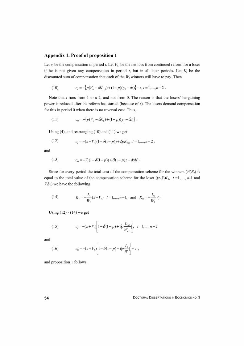
DOCTORAL DISSERTATIONS IN ECONOMICS NO. 3 54
Appendix 1. Proof of proposition 1
Let ct be the compensation in period t. Let Vl,t be the net loss from continued reform for a loser if he is not given any compensation in period t, but in all later periods. Let Kt be the discounted sum of compensation that each of the Wt winners will have to pay. Then
(10) { } 2,....,1,))(1()( 1 −=−−−+−−= + ntzzypKVpc ltwt δδ .
Note that t runs from 1 to n-2, and not from 0. The reason is that the losers’ bargaining power is reduced after the reform has started (because of z). The losers demand compensation for this in period 0 when there is no reversal cost. Thus,
(11) { }))(1()( 10 zypKVpc lw δδ −−+−−= .
Using (4), and rearranging (10) and (11) we get
(12) 2,....,1,))1(1)(( 1 −=+−−+−= + ntpKpVzc tlt δδ ,
and
(13) 10 )1())1(1( pKzppVc l δδδ +−+−−−= .
Since for every period the total cost of the compensation scheme for the winners (WtKt) is equal to the total value of the compensation scheme for the loser ((z-Vl)Lt, t =1,…, n-1 and VlLo) we have the following
(14) ll
t
tt V
WLKntVz
WLK
0
00and,1,....,1)( −=−=+−= .
Using (12) - (14) we get
(15) 2,....,1,)1(1)(1
1 −=
+−−+−=
+
+ ntWLppVzc
t
tlt δδ
and
(16) zWLppVzc l +
+−−+−=
1
10 )1(1)( δδ ,
and proposition 1 follows.

CH. 4 ON THE DYNAMIC CONSISTENCY OF REFORM AND COMPENSATION SCHEMES 55
Appendix 2: Why compensate all losers?
We assume that income is transferable between the individuals and that no-one is liquidity constrained. The bargaining game between the individuals is as follows: In each period the individuals are either sure winners from reform or uncertain (losers) as described in section 2. Their payoffs and status is defined by the process described in section 2. The timing of events is as in section 2, but after the winners have decided the size of the compensation to each of the losers they want to compensate, the uncompensated losers can “bribe” any of the compensated losers to make them pay back the compensation in exchange for voting for reversal (against reform). Then it is voted on whether the reform should be continued (started) or not. Within each period the losers’ voting promise (in exchange for compensation or a bribe) is binding. There is complete information. Decisions are made by majority, but if there is a tie there is no reform (reversal).
We start by looking at the situation in period n-1. Assume that the winners compensate a share m of N, N=L+W, all compensated are losers, and m≤L. To get a winning coalition the winners must set m such that W+m>1/2. If there is a continued reform, each of the uncompensated losers have a total loss of lV− (remember that Vl<0). Thus, each uncompensated loser is indifferent between continued reform and bribing the compensated losers in exchange for reform if the bribe contribution from each uncompensated loser is smaller than or equal to ( )zVl +− . The total amount available to pay in bribes is then
[ ]( )zVmL l +−− . The share of N the uncompensated losers have to bribe to get a majority against reform is 2/1−+ mW . Thus, the compensation needed by each compensated loser to stay in the pro reform coalition is
( ) ( )( )
( )( ) ( )( ) 12
21 −+
+−=+−+−+
−+−mW
zVzVmW
mLzV lll , ( )
21>+ mW .
The last term of the sum on the left hand side is what is demanded by each loser in the pro-reform coalition to stay indifferent over reform and reversal. The first term in the bracket is the total amount that the uncompensated losers are willing to use on bribes divided by the share of N they have to bribe. The equality follows from the fact that (L-m)+(W+m-1/2)=1/2. Total compensation needed to the compensated losers is then
( ) ( )
−++−
121mW
zVm l .
By differentiation of this expression with respect to m we get

DOCTORAL DISSERTATIONS IN ECONOMICS NO. 3 56
( ) ( )( )21212−+
−+−mW
WzVl ,
which is negative as long as there is a minority of winners. Thus, the total compensations that have to be paid is smaller the larger is m, and setting m=L is optimal in period n-1. Since all losers have the same loss from reform, there is nothing to gain by paying different compensation to the compensated losers.
Knowing that all losers will be compensated in period n-1, we can pursue the same analysis for the preceding periods, and it follows that all losers will be compensated in each period.

CH. 4 ON THE DYNAMIC CONSISTENCY OF REFORM AND COMPENSATION SCHEMES 57
References Acemoglu, D and J. A. Robinson (2000), “Political losers as a barrier to economic
development,” AEA Papers and Proceedings, vol. 90, no. 2. Asheim, G. B., C. A. Claussen and T. Nilssen (2002), “Simple majority leads to unanimity,”
under preparation. Baron, D. P. (2001), “Theories of strategic nonmarket participation: majority-rule and
executive institutions,” Journal of Economics and Management Strategy, vol. 10, no. 1. Drazen, A. (2000), Political Economy in Macroeconomics, Princeton University Press. Fernandez, R. and D. Rodrik (1991), “Resistance to reform: Status quo bias in the presence of
individual-specific uncertainty,” American Economic Review, vol. 81, no. 5. Friedman, J. (1986), Game Theory with Applications to Economics, Oxford University Press. Groseclose, T. and J. M. Snyder (1996), “Buying supermajorities,” American Political
Science Review, vol. 90, no. 2. Lau L. J., Y. Qian and G. Roland (2000), "Reform without losers: An interpretation of
China’s dual-track approach to transition", Journal of Political Economy, vol. 108, no. 1. Lau L. J., Y Qian and G. Roland (1997), "Pareto-improving economic reforms through dual-
track liberalization," Economics Letters, vol. 55, no. 2. Rodrik, D. (1996), “Understanding economic policy reform,” Journal of Economic Literature,
vol. 34, no. 1. Rodrik, D. (1999), “Institutions for high quality growth: What they are and how to acquire
them,” NBER Working Paper Series, no. 7540. Roland, G. (2000), Transition and Economics. Politics, Markets and Firms, MIT Press. Saint Paul, G. (1996), “On the political economy of labor market flexibility,” in NBER
Macroeconomics Annual, MIT Press. Tommasi, M and Velasco, A. (1996), “Where are we in the political economy of reform?”
Policy Reform, vol. 1, no. 2.

DOCTORAL DISSERTATIONS IN ECONOMICS NO. 3 58
CH. 5 THE TIME-CONSISTENCY OF TWO-TIER LABOR MARKET REFORMS 59
Chapter 5
The time-consistency of two-tier labor market reforms*
Carl Andreas Claussen**
Norges Bank
Abstract
High layoff costs are often blamed for the high levels of unemployment in Europe. Reforms aimed at reducing these costs nevertheless are rare, possibly because the employed extract rents from these costs. A potential way around this problem is to allow those already employed to keep extensive job protection, while permitting more flexible terms on new contracts. The current literature suggests that a time-consistency problem limits the scope for such a reform. This paper shows that there is no time-consistency problem if there is no fiscal illusion. Thus, reforms that make the link between labor market policies and taxes more transparent and reforms that reduce firing costs are complementary.
Keywords: Dynamic Political Economy, Firing Cost, Reform, Time-consistency, Unemployment JEL Codes: D72, D78, E24.
* Thanks to Geir Asheim for helpful guidance. The research was done when I was visiting the IMF, and the Stockholm School of Economics in spring 2001. I gratefully acknowledge their hospitality. Thanks also to Norges Bank for financial support. Remaining omissions and mistakes are mine. The views presented are mine and do not necessarily represent those of Norges Bank.
** [email protected] Norges Bank, box 1179 Sentrum, 0107 Oslo, Norway.
DOCTORAL DISSERTATIONS IN ECONOMICS NO. 3 60
1. Introduction
Labor market rigidities such as high layoff costs are often blamed for the high and persistent unemployment levels in Europe (see e.g. OECD (1994)). However, significant reforms to reduce these rigidities are rare. Why is that? From modern labor market theory we know that rigidities make it possible for the employed to extract rents. Consequently, the absence of reforms could be due to opposition from the employed.
One way around this problem could be to allow those already employed to keep their privileges i.e. extensive job protection, while permitting more flexible terms on new contracts. Saint-Paul (1996, 2000) examines this idea formally and finds that a time-consistency problem limits the scope for such reforms. Roughly the argument is as follows: it is likely that there are some extra costs to workers from a two-tier system compared with a system where all contracts are flexible (costs from monitoring, etc). Furthermore, over time the number of workers on flexible contracts increases so that, as a result of reform, the political power gradually changes in favor of workers on more flexible contracts. Consequently, those employed on rigid contracts will know that at some time in the future they will lose their political power and all contracts will be made flexible. This implies that they expect to lose their privileges at some time in the future. They therefore demand more (implicit) transfers to accept reform, and this limits the scope for reform.
However, Saint-Paul uses a partial equilibrium model. Dynamic effects of unemployment levels on taxes are not taken into account. Usually the employed pay taxes to finance unemployment benefits and other costs of unemployment like lost output. When these costs are taken into account, reduced layoff costs have two opposing effects on the utility of the employed. On the one hand, it reduces the possibility of the employed to extract rents, but on the other hand it reduces the taxes the employed have to pay.
In this paper we pursue the following hypothesis: if the tax effect of reduced unemployment is taken into account, the time-consistency problem discovered by Saint-Paul disappears.
To test this hypothesis we add tax-financed unemployment benefits and a balanced budget constraint to the Saint-Paul model. We find that there is no time consistency problem in this model. Two dynamic features give this result. First, as Saint-Paul (2000) points out, employment tends to overshoot its post reform steady state level during transition. Second, the initial reduction in unemployment is faster, and the later increase from an overshoot level is slower under a two-tier reform than under a complete reform where all contracts are made flexible in one shot. Both effects imply a lower cost of financing the unemployment scheme under the two-tier regime than

CH. 5 THE TIME-CONSISTENCY OF TWO-TIER LABOR MARKET REFORMS 61
under a complete reform. Consequently, workers on flexible contracts also prefer to keep the two-tier system even though there are some extra costs for administering it.
Our findings indicate that better knowledge among the electorate about the tax implications of labor market policies make a two-tier reform more efficient politically than suggested by the literature so far. The findings also point to a complementarity of i) a reform that renders visual the cost of the unemployment scheme and ii) a reform that reduces rigidities in the labor market. It also suggests sequencing the reforms so that i) is done/proposed before ii).
Our paper is related to two different kinds of literature: the modern “matching” equilibrium unemployment theory, and the literature on the political economy of reform.
In the modern “matching”-equilibrium unemployment theory, search both by employers and workers leads to an equilibrium number of job matches and an unemployment rate. The theory is thoroughly presented in Pissarides (2000). We analyze a political-economic situation with dynamic strategic interaction between the employed on flexible contracts, the employed on rigid contracts and the unemployed. The preferences of each type are unchanged over time, but the employment status of each individual might change. The matching framework makes this rather complicated situation analytically tractable.
The heart of the literature on the political economy of economic reform is a puzzle similar to the one motivating our exercise; why is a welfare-enhancing reform not implemented? Our paper is part of the normative variety of this literature. Like Dewatripont and Roland (1992, 1995) and Wei (1997) among others, we argue that partial reform is a potential way around the problems leading to non-adoption. The two-tier reform can also be understood as an implicit compensation mechanism. Recent contributions in a similar vein are Lau et al. (1997, 2000). They discuss the dual track approach to market liberalization as a mechanism for implementing reform and achieving efficiency without creating losers. Rodrik (1996), Tommasi and Velasco (1996), and Drazen (2000) have surveyed the modern literature on the political economy of reform.
The paper is organized as follows. We present the basic model in section 2. We divide the presentation of the model into five sub-sections. In section 2.1 we present the more economic aspects of the model. Then we introduce the politics in section 2.2. Section 2.3 provides the information structure and the timing of events. In section 2.4 we put restrictions on the model to tailor it to the situation we want to describe, namely a situation where reducing firing costs will reduce unemployment, but where a majority of the voters oppose a uniform reduction in firing costs. In section 2.5 we put the pieces together. In section 3 we first briefly look at a complete reform where the changes in firing costs apply to both new and old contracts and then move on to analyze a two-tier reform where reductions in firing costs only apply to contracts entered into after

DOCTORAL DISSERTATIONS IN ECONOMICS NO. 3 62
reform. In section 4 we discuss possible time-consistency problems, and show that they are non-existent in our model. Here we also briefly discuss some of our assumptions. We conclude with section 5.
2. Basic model
In this section we describe the basic model. The model is based on the model by Saint-Paul (1996) (SP hereafter). We will be explicit when we introduce new elements and ideas to the model. The main difference will be the explicit budgetary link between the total cost of unemployment benefits and taxes levied on the employed. Since unemployment levels depend on labor market policies, this means that we introduce a link between labor market policies to taxes. 2.1 The economics
Our description of the labor market focuses on flows in and out of employment. We assume that a constant share of the unemployed flows into employment. Similarly, a constant share of the employed flows into unemployment. The two shares are assumed only to depend on the cost of firing workers. This specification is based on the Pissarides (2000) matching-type equilibrium unemployment theory, where the constant shares and their dependence on the firing cost follows endogenously (see Saint-Paul (2000)).
More concretely, let q be the cost of firing a worker. At every unit of time a share
(1) s = s(q), s’(q) < 0,
of the employed is fired and a share
h = f(q), f’(q) < 0,
is hired. Since s(q) is monotonically increasing, we have that q = s-1(s), and the hiring per unit of time is
(2) h = h(s), h’(s)>0.
The relationship between the firing cost and the firing rate given by (1) implies that we can consider the firing rate s to be the policy parameter.
In addition to the flow in and out of employment/unemployment, there is a constant flow of a share p of the working-age population into retirement. At the same time, p new workers enter the labor force so that the total size of the working age population is constant. Retirement is out of both work and unemployment whereas all new workers enter into unemployment.

CH. 5 THE TIME-CONSISTENCY OF TWO-TIER LABOR MARKET REFORMS 63
The development of the share of employed (l) and unemployed (u) over time is then
(3) lpsushdtdl )()( +−= ,
and
(4) upshpsldtdu ))(( +−+= .
The steady state share of employed and unemployed is thus (use l+u=1)
(5) pssh
shl++
=)(
)( ,
and
(6) pssh
spu++
+=)(
.
We now turn to the utility of the employed and unemployed. The employed continuously receive a wage w and the unemployed receive a benefit ω. The wage and the benefit is fixed and independent of the firing cost. A fraction τ of the wage is taxed. With a perfect capital market, infinite horizon, no expectations of changes in the parameters in the model and risk- neutral individuals, the expected present value of the income streams (utility) for the employed ( uV ) and the employed ( eV ) are described by the following two Bellman equations:
(7) euee pVVVswrV −−−−= )()1( τ ,
and
(8) uueu pVVVshrV −−+= ))((ω .
From these two equations we can solve for the expected present values for the employed and unemployed. This gives us
(9) ( )( )( ))(
)1()(shsprpr
wshprsVe ++++−+++= τω ,
and
(10) ( )( ))()1()()(
shsprprwshsprVu ++++
−+++= τω .

DOCTORAL DISSERTATIONS IN ECONOMICS NO. 3 64
So far the model is similar to SP’s model except that there is no explicit tax in SP’s model. We will now introduce the main difference, the budget constraint, making τ endogenous. We assume that unemployment benefits are fully financed by taxes on the employed. Furthermore, we assume that individuals fully understand the inter-temporal budgetary link between unemployment benefits, the number of unemployed, and the taxes levied on the employed, i.e. there is no fiscal illusion. This is a reasonable assumption in this model since there is only individual-specific uncertainty: individuals do not know their employment status in the future, but they can calculate the aggregate share of unemployed and employed in the working-age population. It is therefore possible for them to calculate the present value of future unemployment benefits for any firing rate.
More concretely, the present value of the total unemployment benefits (C) is
C = )(tUω ,
where
∫∞
−≡t
rz dzzuetU )()( .
The inter-temporal budget constraint is then:
∫∞
− −=t
rz dzzuewtU ))(1()( τω ,
where the constant tax rate τ is set in such a way that the budget constraint is fulfilled. That is,
(11) ( ))(1)(
)()(
)(tUre
tUrew
tUdze
tUw rt
rt
t
rt −=
−
=
∫∞
−
ωωτ .
This specification with a constant tax rate makes the model relatively easy to handle. The alternative assumption with a “pay-as-you-go" financing of unemployment benefits would have made Ve and Vu functions of time, and complicate the analysis considerably. Our specification with a constant tax rate also rules out questions concerning distribution of the tax burden over time, and thereby isolates the pure budgetary links.
With this set-up, there might be some borrowing for some time if unemployment is high and fall in the future. Similarly, there might be saving for some time if unemployment will rise in the

CH. 5 THE TIME-CONSISTENCY OF TWO-TIER LABOR MARKET REFORMS 65
future. If there has been no previous borrowing or saving the steady state level of taxes is given by
(12) lu
wωτ = .
2.2 The politics
The following simplifying assumptions are made about the politics: There is
• majority voting,
• only members of the working age population can vote, and
• the only issue considered is the labor market policy (firing costs).
• There is voting continuously.
The first assumption simplifies the analysis but qualitatively the results would apply to other political systems where the political influence of workers on rigid contracts depends on their share in total employment. The second assumption is reasonable given that in any country most voters in the working-age population. The third assumption is strong, but in line with the tradition in the literature.
2.3 Timing of events and information structure
At every instance of time, workers are fired, retired, or hired, new workers enter the unemployment pool, the employed receive their wage, and there is voting about the labor market policy. At time t=0, it is voted on whether to start reform and what sort of reform to start. There are two alternatives. A complete reform where the changes in firing costs apply to all existing and new contracts, or a two-tier reform where changes in firing costs apply to new contracts only. For t>0 it is voted on whether to continue the two-tier reform if that was initiated at t=0, or whether there should be a switch to a complete reform. Any change in the labor market policy is implemented from the ‘next’ instance.
There is complete information. 2.4 Restricting the model
As it now stands the model captures a wide range of situations. To tailor the model to situations where reducing the firing cost (increasing the firing rate) reduces unemployment, but where a majority opposes such a policy, restrictions have to be placed on the parameters and the functional

DOCTORAL DISSERTATIONS IN ECONOMICS NO. 3 66
forms. We start by presenting the restrictions, and then explain how they give the features we want. Let sR be the pre-reform firing rate.
R1. ω
+−>)(
1 R
R
shpsw
R2. pssh RR +>)(
R3. h”<0
R4. )0(')0(
hhp >
Restriction R1 ensures that it is better to be employed than unemployed (i.e. Ve > Vu). We can see this the following way. Using (9) and (10) we get the following criteria for Ve > Vu:
ωτ >− )1(w .
Substituting for τ from (12) and for l and u from (5) and (6) we get R1. Restriction R2 is necessary for there to be a majority of employed in steady state. We see this
from (5). Restriction R3 states that “the gains from greater flexibility are larger when the labor market is
more rigid to start with.”(SP, p. 156) This is a reasonable assumption for at least some range for s. The assumption implies that the employed are against any increases in the firing rate if unemployment has no effect on taxes. To see this we differentiate (9) partially (setting 0' =sτ ) and get
(13) ( )( )( )( )2)(
))(()(')1(shsprpr
shprsshws
Ve
++++++−−−=
∂∂ ωτ .
To find the sign of this expression we use R3 and the fact that there cannot be negative hiring ( 0)0( ≥h ), and have
0)(')( >− sshsh ,
which together with R1 imply that
(14) 0<∂
∂s
Ve .

CH. 5 THE TIME-CONSISTENCY OF TWO-TIER LABOR MARKET REFORMS 67
Restriction R4 is necessary for there to be an interval for s where increasing s leads to a reduction in steady state unemployment.1 We can see this by differentiating (6), which gives
(15) ( )2)())((')(
spshpsshsh
dsud
+++−= .
Differentiating the nominator in (15) we have
))(('' pssh +− ,
which by R3 is always positive. Thus, the nominator is increasing in s, and can only be negative for some interval for s if
00
<=s
dsud ,
which is the same as
0)0(')0( <− phh .
Note also that p > 0 is necessary for there to be a range where increasing s reduces unemployment. This further suggests the following definition, which will also be helpful later. Let
minus be defined by 0))((')( minminmin =+− psshsh uuu (c.f. (15)).
Definition
There is full employment if l )(1 minusu−= .
Restriction R4 also implies that there is an interval for s where increasing s increases the utility
of the unemployed when there are no tax effects. To see this we first differentiate (10) partially (holding τ constant), and get
(16) ( )( )( )( )2)(
)()´()()1(shsprpr
shshsprws
Vu
++++−++−−=
∂∂ ωτ .
1 The effect of firing costs on unemployment is debated in the literature. See Ljungquist (2001) for an overview of this discussion.
DOCTORAL DISSERTATIONS IN ECONOMICS NO. 3 68
By comparing the nominator in (16) and (15) we see that if there are no tax effects, the unemployed are in favor of any marginal increase in the firing rate as long as it reduces unemployment. Thus
0min >∂
∂⇒≤
sVss uu .
2.5 Putting the pieces together
We will here put the pieces together. The total effect on utilities from a change in the firing rate is
(17) dsdV
sV
dsdV eee τ
τ∂∂+
∂∂= ,
and
(18) dsdV
sV
dsdV uuu τ
τ∂∂+
∂∂= .
Thus, the total effect of changes in s is the sum of the direct effect given by (13) and (16), and the indirect effect that works through changes in the tax rate. From (13) and (16) we know how the direct effects depend on the initial firing rate. The indirect effects are given by the following:
( )( )( ) s
e
shsprprshprw
dsdV '
)()( ττ
τ ++++++−=
∂∂ ,
( )( ) su
shsprprshw
dsdV '
)()( ττ
τ ++++−=
∂∂ .
We see that the indirect effects are positive if taxes are reduced when s is increased and negative if the tax rate increases. From (11) we know that what happens to the tax rate depends on what happens to unemployment. Consequently, we have that
minifonly and if0 ue ssdsdV <>
∂∂ τ
τ,
and
minifonly and if0 uu ssdsdV <>
∂∂ τ
τ.

CH. 5 THE TIME-CONSISTENCY OF TWO-TIER LABOR MARKET REFORMS 69
We can now draw the following conclusions regarding the total effects on individuals’ utilities from changes in the firing rate.
(19) 0<ds
dVe for minuss ≥
and
(20) 0>ds
dVu for minuss ≤ .
Now, let maxeVs be the firing rate that maximizes the expected utility for the employed and maxuVs be the firing rate that maximizes the expected utility for the unemployed. Then, from (19) it follows that
(21) minmax uV ss e < ,
and from (20) we have that
(22) minmax uV ss u ≥ .
Figure 1 illustrates what we know so far.

DOCTORAL DISSERTATIONS IN ECONOMICS NO. 3 70
From (9) and (10) we see that Ve>0 and Vu>0 if τ<1. From (12) we see that τ<1 (as long as there is no debt to service). The Ve-line is dotted to the left of maxeVs to reflect that we do not know whether an interval exists for s such that dVe/ds>0. Note also that if no interval exists for s such that dVe/ds>0, then 0max =eVs . We have not drawn the Vu-line to the right of minus , reflecting that we do not know much about the slope of the function in this interval. All we know is that maxuVs has to be to the right of minus (as indicated).
The area where reducing the firing rate to reduce unemployment is politically difficult is shaded in the figure. We assume that the initial firing rate sR is in this area. That is, we assume that there is room for a reduction in unemployment by increasing the firing rate and that the initial firing rate is such that the employed are against any increase in the firing costs connected to their contract.
A1. [ )minmax , uVR sss e∈ .
3. Reform
A complete reform, i.e. a reform where reductions in firing costs apply to all existing and new labor contracts, will of course be opposed by the majority of employed when R1-R4 and A1 hold (c.f. fig. 1).
Figure 1. Unemployment and utility of employed and unemployed for different firing rates
Ve , Vu ,
maxuVsmaxeVs
_u
Ve
Vu
_u
sminus

CH. 5 THE TIME-CONSISTENCY OF TWO-TIER LABOR MARKET REFORMS 71
We will here show how a two-tier reform makes it politically possible to achieve full employment even under A1. Let sF be the firing rate on new contracts suggested by the government and let
A2. minuFR sss ≤< .
The unemployed are in favor of any reform where s is reduced to sF, c.f. fig 1.2 For the employed, we must remember that under the two-tier reform the firing rate linked to their job is unchanged as long as they stay employed. We therefore start from (7). Rearranging terms we get
[ ]ue sVwpsr
V +−++
= )1(1 τ .
By plugging in sR and differentiating τ and Vu with respect to s we get the following:
(23)
+−
++=
dsdVs
dsdw
psrdsdV uR
Re τ1
reform tier two
.
We already know that dVu/ds>0. We also know that steady state unemployment will fall, and this implies that taxes will fall. We can therefore conclude that the employed will be in favor of this reform.
The intuition behind this feature of a two-tier reform is the following: since the firing rate is not changed for the employed, they keep their privileges. The chance of losing their job is unchanged. Additionally, they have lower taxes when employed and higher utility if they become unemployed. Thus, also in our version of the SP-model a two-tier reform strategy is an efficient way of overcoming political opposition against increases to the firing rate that reduces employment.
4. The time-consistency of two-tier reforms
Before we can continue we need a precise definition of what we mean by the time-consistency problem. Let t* be the time when workers on rigid contracts first are in minority under a two-tier reform. Let C
eV and CuV be the net discounted utility for the employed on flexible contracts and
2 Formally the preference of the unemployed over such a two-tier reform is both in the case of complete reform and a two-tier reform given by (18). R1-R2, A1 and A2 ensure that the unemployed are in favor of such a reform.

DOCTORAL DISSERTATIONS IN ECONOMICS NO. 3 72
the unemployed if a complete reform is pursued. Similarly, let TeV and T
uV be the net discounted utility for the employed on flexible contracts and the unemployed if a two-tier reform is pursued.
Definition (time-consistency problem)
There is a time-consistency problem if CeV > T
eV and CuV > T
uV for t>t*.
So far, we have assumed that there are no additional costs incurred by the dual labor market
regulations. Thus, the expected utilities of workers on flexible contracts and the unemployed are independent of whether there is full reform or continued two-tier reform. Consequently, there is no reason to change from a two-tier reform to a complete reform.
It might be more reasonable to assume that the two-tier system gives rise to some extra monitoring or supervision costs. We will now see what happens if we introduce these extra costs. As does SP, we add the following assumption to our model: A3. There is a small resource cost from monitoring a two-tier labor market. This cost falls in
equal shares on all individuals. The weight on this cost in the individuals’ utility function is small; of two outcomes, the one that yields the higher expected discounted income is preferred. In case of a tie, the one with the lowest monitoring cost is preferred.
SP shows that in his version of the model this assumption introduces a time-consistency
problem limiting the scope for reform. The intuition is the following: for workers on flexible contracts and the unemployed A3 makes a complete reform preferable to a two-tier reform. Workers on the more rigid contracts therefore know that a proposal for a full reform will be accepted when t≥t*. The gain from a two-tier reform is therefore reduced, and the consensus role of the two-tier reform is reduced.
We will now show that this result does not hold in our version of the model. We will first give the intuition behind this result, and then the formal proof.
Since the steady state unemployment is lower for s=sF than s=sR, we know that unemployment will have to fall following reform. If this fall is faster under a continued two-tier reform than under a complete reform, completing the two-tier reform gives lower unemployment during the transition and thereby a lower tax rate.
In our model unemployment falls faster with the continuation of a two-tier reform than under a complete reform. The reason is the following. Under a two-tier reform some of the employed
CH. 5 THE TIME-CONSISTENCY OF TWO-TIER LABOR MARKET REFORMS 73
workers are still on rigid contracts, whereas under a complete reform all employment is on flexible contracts. This means that for the same level of employment firms cannot fire as large a share of the workers under a two-tier reform as under a complete reform. Thus, net hiring must for the same level of unemployment be higher under a two-tier reform than under a complete reform. Consequently, unemployment falls faster under a two-tier reform than under a complete reform.
These effects tend to make unemployment reach the new steady state level before all employment is on flexible terms. Consequently, employment will overshoot (unemployment “undershoot”). We therefore have to check if unemployment increases more slowly from “undershoot” levels under a two-tier reform than under a complete reform. In our model the increase in unemployment is slower under a two-tier reform than under a complete reform. It is the same effects as in the previous paragraph that give this result: for the same level of unemployment the hiring is the same under a complete and a two-tier reform, but the firing is smaller under a two-tier reform as long as there are workers still employed on rigid contracts.
We therefore have that
Proposition
Under R1-R4 and A1-A3 there is no time-consistency problem, i.e. there will be unanimous support for a continued two-tier reform as long as there are still workers employed on rigid contracts.
Proof
The change in the shares of employed on rigid terms ( Rl ), on more flexible terms ( Fl ) and the share of unemployed (u) under a two-tier reform are given by
(24)
RRR
FFFRR
FFFF
lpsdt
dl
pupshlslsdtdu
lpsushdt
dl
)(
))((
)()(
+−=
++−+=
+−=
,
Since ull FR ++=1 , the developments and the steady state solutions to the system can be described in a two-dimensional phase diagram. The demarcation curve for du/dt=0 is given by

DOCTORAL DISSERTATIONS IN ECONOMICS NO. 3 74
FR
F
FR
FFR
sspsu
ssspshl
−+−
−++= )( .
The dlR/dt=0 curve is a straight line on the horizontal axis. The phase diagram is illustrated in figure 2 where the bold lines give the demarcation lines. The directional arrows show that the steady state point is a stable node. The line marked “ 1≤+ ul R ” gives the upper boundary for the variables. Any initial steady state point must be on this line.
The phase diagram shows that unemployment falls during the transitional phase when Fuu > .
Using (4), (24) setting ulull FR +=++ we get that unemployment falls faster under a two-tier reform than under a complete reform since with R1-R4 and A1-A2 we have that
(25) ( ) 0reformtiertworeformcomplete
>−=−−
RRF lssdtdu
dtdu .
The phase diagram shows that after unemployment has reached its minimum level, it will increase until it reaches the new steady state level. Equation (25) shows that unemployment increases more slowly under a two-tier reform than under a complete reform when Fuu < and
0/ >dtdu . This implies that whether there is overshooting or not
reformtier Two-reformComplete)()( tUtU > as long
as 0>Rl . This implies that (use (11)) reformtier -TworeformComplete ττ > as long as 0>Rl . If 0=Rl , a
two-tier reform is irrelevant. Consequently, CeV < T
eV and CuV < T
uV for t>0. Q.E.D.
Figure 2. Phase diagram for two-tier reform
lR
u
1=+ ul R
Fu
0=dt
dl R
0=dtdu
)( maxeVR Su

CH. 5 THE TIME-CONSISTENCY OF TWO-TIER LABOR MARKET REFORMS 75
We have assumed that there is continuous voting on whether to pursue a two-tier reform or a complete reform, and implicitly assumed that a reversal for the entire reform is never considered. From the preferences revealed in figure 1 it follows that if it were possible to reverse the entire reform at any time, it would happen as soon as there was a majority on flexible contracts. It is in the interest of the workers on flexible contracts to change the firing rate to maxeVs for all the employed immediately. The employed on rigid contracts will be against since they have higher utility under a continued two-tier reform (c.f. last paragraph of section 3.) Thus, under a more realistic assumption the “flexible” steady state equilibrium is unstable, indicating that there will be cycles in the labor market policies. We have chosen not to focus on these aspects to highlight our main argument, i.e. that there is no time-consistency problem in the SP-model (SP has also (implicitly) ruled out reversal).
Another apparently strong assumption we have made is that wages are fixed and unrelated to unemployment and labor market legislation and unemployment levels. All the rents from employment protection (high firing rates) are achieved by the low probability of losing one’s job. More realistically wages would depend on the level of job protection. Again we have followed the assumptions made by SP. However, we believe changing this simplifying assumption has little effect on our main conclusion.
The size of the cost of monitoring the different systems and the cost of switching between them is relevant for the results. Incorporating this in the analysis is straightforward, and would not change our main conclusion as long as the monitoring cost and the cost of changing the firing rate is not too high. The dynamics would be somewhat more complicated however. We leave this exercise for later analysis.
5. Conclusion
In this paper we have studied a two-tier reform on the labor market. Two-tier reforms are reforms where reductions in firing costs apply only to new labor contracts. For contracts entered into before the reform, firing costs are unchanged. This reform makes it possible to achieve full employment even though the majority of employed would lose from a reform where all contracts were made more flexible. The reason is that by allowing for existing rigid contracts to remain rigid, the losers from reform are compensated implicitly.
In contrast to previous work we have included an explicit budgetary link between labor market policies to taxes, thereby bringing the analysis closer to a general equilibrium analysis. We find

DOCTORAL DISSERTATIONS IN ECONOMICS NO. 3 76
that the time-consistency problem found in previous work disappears when this more realistic assumption is included.
Our work is normative in spirit, and we can draw several conclusions for reform policies that reduce firing costs. The first is that a two-tier reform could be an efficient tool for overcoming political opposition to reductions in firing costs even if it results in an extra “monitoring” cost compared with a reform where changes in legislation (firing costs) apply to all contracts. This conclusion rests on the general equilibrium effect linking unemployment policies and taxes levied on the employed. A conclusion following this is that there is a complementarity between a reform that renders visible the cost of the unemployment scheme and a reform that reduces rigidities on the labor market. It also suggests the following sequencing of reforms: first make the cost of the unemployment benefit scheme and the link between labor market policies and taxes more transparent and well known among the voters, then propose the reduction in firing costs.

CH. 5 THE TIME-CONSISTENCY OF TWO-TIER LABOR MARKET REFORMS 77
Literature Coate, S. and S. Morris (1995), ”On the form of transfers to special interests,” Journal of Political
Economy, vol. 103, no. 6. Dewatripont, M. and G. Roland (1992), “Economic reform and dynamic political constraints,”
Review of Economic Studies, vol. 59, no. 4. Dewatripont, M. and G. Roland (1995), “The design of reform packages under uncertainty”,
American Economic Review, vol. 85, no. 5. Drazen, A. (2000), Political economy in macroeconomics, Princeton University Press. Lau L. J., Y. Qian and G. Roland (1997), "Pareto-improving economic reforms through dual-track
liberalization," Economics Letters, vol. 55, no. 2. Lau L. J., Y. Qian and G. Roland (2000), "Reform without losers: An interpretation of China’s
dual-track approach to transition", Journal of Political Economy, vol. 108, no. 1. Ljungqvist, L. (2001), “How do layoff costs affect employment?” Mimeo, Stockholm School of
Economics, February. OECD (1994), The OECD Jobs Study: Evidence and Explanations. Rodrik, D. (1996), “Understanding economic policy reform,” Journal of Economic Literature,
Vol. 34, no. 1. Saint-Paul, G. (1996), “On the political economy of labor market flexibility”, in NBER
Macroeconomics Annual, MIT Press. Saint-Paul, G. (2000), The Political Economy of Labor Market Institutions, Oxford University
Press. Pissarides C., A. (2000): Equilibrium Unemployment Theory, MIT press. Tommasi, M and Velasco, A. (1996), “Where are we in the political economy of reform?” Policy
Reform, vol. 1, no. 2. Wei, S-J. (1997), “Gradualism versus big bang: Speed and sustainability of reforms,” Canadian
Journal of Economics, Vol. 30, no. 4.

15480
ISSN 1503-0741
ISBN 82-7553-216-7