Four bagatelles on channel growth

Quatre observations sur la croissance des ravines de sape

Alexander P. Petroff ∗, Olivier Devauchelle ∗†, Arshad Kudrolli ‡, and Daniel H. Rothman ∗

20 juillet 2011

Resume

Les ravines creusees par le suintement d’un aquifere forment parfois un reseau ramifie, dontla dynamique peut etre comprise simplement. Elles constituent ainsi un systeme naturel propicea l’etude de la croissance des reseaux. Nous presentons ici trois facettes de cette dynamiquesimple, qui permettent d’etablir une theorie quantitative de la formation d’un reseau de drainagenaturel a l’echelle du kilometre. En trois sections distinctes, nous nous efforcons de relier le debitd’eau qui s’ecoule dans une riviere a la geometrie du reseau, de comprendre la forme du profild’elevation de ces rivieres, et l’influence de l’ensoleillement de la topographie sur l’erosion duplateau dans lequel croissent les ravines. Dans chaque cas, nous proposons une comparaisonquantitative avec des mesures in situ.

Abstract

Networks fed by subsurface flow are a natural, but dynamically simple, system in which to consi-der general problems of network growth. Here we present three examples in which this dynamicsimplicity can be used to develop a quantitative understanding of a natural kilometer-scalenetwork of streams. In these three sections, we investigate the relation between the position ofa spring in the network and the groundwater flux into it, the flow of water through streams andthe stream shape, and the influence of solar radiation on the rate of sediment transport aroundthe streams. In each case a quantitative comparison is made between theory and observation.

Keywords : Geomorphology, hydrology, rivers network

Mots cles : Geomorphologie, hydrologie, reseaux de rivieres

1 Introduction

When rain falls on a sandy landscape, itflows into the aquifer, eventually re-emerging

∗. Lorenz Center, Department of Earth, Atmosphe-ric and Planetary Science, Massachusetts Institute ofTechnology, Cambrigde, MA, USA†. Institut de physique du globe de Paris – Sorbonne

Paris Cite, Universite Paris Diderot, UMR CNRS 7154‡. Department of Physics, Clark University, Worces-

ter, MA, USA

into streams. As groundwater flow accumulatesin streams, sediment is removed and the land-scape is eroded. This interplay between sub-surface flow, erosion of the surrounding land-scape, and the removal of sediment throughstreams causes existing stream heads to growforward and new streams to form. In this way,groundwater-fed streams grow into ramifiednetworks [1].

Proposed examples of these so-called seepage

1

channels can be found on both Earth [2–4]and Mars [5]. Of these systems, a seepage net-work on the Florida Panhandle stands out asa superb example of the type. A topographicmap of the network is shown in figure 1 [6].This kilometer-scale network is incised into a65m deep bed of sand overlying an imper-meable layer of muddy marine carbonates andsands [4]. Groundwater flows through the sandabove the impermeable substratum, into thenetwork of streams, and drains into a nearbyriver [4, 6].

The dynamics shaping groundwater-fed net-works are simpler than the more common typeof drainage networks that are fed by overlandflow. In particular, the flow of the groundwaterinto streams is determined by the shape of thewater table, which is a solution to a Poissonequation [7]. Because the growth of a streamsfed by groundwater is an example of networkgrowth in a Poisson field, the analysis of land-scapes shaped by this process benefits froma substantial literature on interface growth ina harmonic fields [8–10]. Past work [11] hasshown that the flow of groundwater into theFlorida network is accurately described by thePoisson equation.

Here we use the specific example of the Flo-rida seepage network to explore the generalconnection between the geometry and growthof drainage networks. This exploration takesthe form of four thematically related, but inde-pendent, exercises in which the dynamic simpli-city of seepage erosion is exploited to developa quantitative understanding of field observa-tions. The focus of this collection is the realiza-tion that groundwater flow and landscape ero-sion are coupled to one another by the streamnetwork and the empirical validation that, closeto equilibrium, this coupling takes a simpleform. Related oddities and novelties are brie-fly discussed.

1 km

10 m 30 m 50 m 70 m

Figure 1 – A kilometer-scale network of see-page valleys from the Florida Panhandle. Thesevalleys are incised tens of meters into unconso-lidated sand. Groundwater flows form the sandbed, through the channels, and through thebluff to the west of the network. Color indi-cates elevation above sea-level.

2 Estimating groundwaterflow from network geometry

We begin by considering a spring, the headof a stream where groundwater first reemergesto the surface. In particular, we compare twomodels that relate the position of a spring inthe network to the flow of water into it.

The first is the continuum model alluded toin the introduction. According to the Dupuitapproximation of Darcy’s Law [7], the waterflux q if related to the height h of the watertable above the impermeable layer as

q = −Kh∇h, (1)

where K is the hydraulic conductivity. Atsteady-state, conservation of mass requires abalance of the precipitation rate P with thedivergence of the flux. Thus, the height of thewater table is a solution of the Poisson equation

K

2∇2h2 = −P. (2)

Because the change in elevation along theFlorida network is small (the median slope

2

1.5 2 2.5 31

1.5

2

2.5

3

3.5

4

log10

(poisson flux) (m)

log

10(g

eo

me

tric

flu

x)

(m

)

Figure 2 – Comparison of the flow into 82springs from the Florida network as estimatedfrom Darcy’s law (“Poisson flux”) and a heu-ristic model (“geometric flux” [6]). The red lineshows the best fitting power-law.

is S ∼ 10−2), we approximate the height ofthe streams above the impermeable layer asconstant. Because this equation is linear inthe variable φ = Kh2/2P , this boundary-valueproblem around the streams of the Florida net-work using the finite element method [11,12].

The second model of subsurface flow is theheuristic Area-driven model [6]. According tothis approximation, all groundwater flows to-wards the nearest section stream. Thus, to findthe flux of water into a section of the net-work, one first identifies the area a around thestreams that is nearer to the selected sectionthan to any other point on the streams. Fromconservation of mass, the discharge of ground-water into this section is Qg = Pa.

We now compare the estimated groundwaterflux in to 82 springs from the Florida network.To do so, it is useful to define two quantities.The Poisson flux qp = ‖∇φ‖. Physically, qpis the area draining into a section of stream

per unit length. By analogy, the geometric fluxinto a section of network of length δs and drai-nage area a is qg = a/δs. Because the Area-driven model allows a finite area to drain intoa point, this definition requires a finite value ofδs, we take δs = 11 m. As shown in figure (2),there is a power law relationship (R2 = 0.94,p < 10−35) between these quantities, qg = Bqαg .The scaling exponent is α = 0.69 ± 0.06. Theproportionality constant, B = 4.0 ± 1.6 m1−α,likely depends on the choice of δs.

Although there is no general quantitative re-lationship between these measures, there is for-mal relationship. Let us imagine that each raindrop falls randomly, with a uniform distribu-tion over the domain, and then undergoes arandom walk until it reaches a boundary. Theprobability distribution of the random walkerspositions satisfies the Poisson equation, whichcan be interpreted as a diffusion equation witha uniform source term [13]. As a consequenceof its random walk through the domain, thisimaginary rain drop has a continuous and non-vanishing probability distribution p of exit lo-cations along the boundary, with a maximumat the closest point on the boundary. The meanflux of walkers through the section of channelsgives the Poisson flux. To find geometric drai-nage area, one sends each random walker to themode of p. Thus, the precise relationship bet-ween qg and qp depends on the geometry of thesystem and, consequently, the scaling exponentα relating these quantities is likely not univer-sal.

We conclude that the Area-driven modelcan be safely used as a conceptual tool withwhich to gain intuition. Nevertheless, the Pois-son equation should be used whenever a quan-titative prediction of the seepage intensity orthe relative fluxes into different parts of thenetwork is required.

3

3 The three dimensionalstructure of the network

Having discussed the flow of water into astream, we now consider the response of sedi-ment within the stream to the flowing water.Flowing water erodes the bottom of the sandystream when the shear force exerted on a sandgrain is sufficient to overcome friction. Thus,there is a threshold that the shear must ex-ceed for any sediment to be transported. [14,15]Many streams, and the Florida network in par-ticular, are thought to adjust to a state inwhich every grain is on the threshold of mo-tion [16–18]. This constraint on the shear canbe re-expressed as to a relationship between theslope of the stream bed S and the discharge Q(units of volume/time) of water in the streamas

QS2 = Q0, (3)

where Q0 is a constant with units of dischargethe value of which depends on parameters suchas the grain size. [16–18].

Because both the discharge of a stream andthe slope effect the flow of groundwater into it,equation (3) imposes a boundary condition forthe flow of groundwater into the streams, fromwhich one can derive the profile of an isolatedstream [18]. Here we show that this boundarycondition is satisfied throughout the network.

To test the applicability of equation 3, wecompare the measured slope of streams to thestream discharge. Estimates of both the slopeand the discharge require a three-dimensionaldescription structure of the drainage network,which is extracted from the high-resolution to-pographic map of the network shown in fi-gure 1. A depiction of part of the network isshown in figure 3. Given the height Hs of eachpoint of the network, the slope is measuredfrom the change in height along the stream.To estimate estimate Q, we first solve equa-tion (2) subject to the boundary condition on

2500

3000

3500

4000

4500

5000

5500

22002700

3200

20

30

40

easting [m]

northing [m]

heig

ht [m

]

Figure 3 – The three-dimensional shape of astream network measured from a topographicmap. Color indicates elevation above sea-level.Streams curve upward sharply near springs.Further downstream, as flow accumulates thestreams become flatter. This inverse relation-ship between slope and discharge is in quanti-tative agreement with equation (3).

the streamsh = Hs. (4)

Because equation (2) is a non-linear functionof h, its solution depends on the height ofthe streams above the impermeable mudstonelayer. The elevation of the impermeable layerabove sea-level is h0 = 0. Figure 4 shows theheight of the water table around the networktaking P = 5 10−8 m/s, K = 1.6 10−5 m/s.Given this solution, Q is estimated throughoutthe network as

Q(x0, y0) = −K∮

N (x0,y0)

h[∂h∂n

]ds, (5)

where N (x0, y0) is the network upstream ofthe point (x0, y0), s is a curvilinear coordinatealong the streams, n is the local normal, and[·] represents the “jump”, which accounts forthe flow of groundwater into either side of theone-dimensional stream.

4

10 m

20 m

30 m

40 m

50 m

Figure 4 – The shape of the water tablearound the Florida network as calculated fromequation (2). Black lines represent the posi-tion of streams. The water table intersectsthe streams at the measured height of thestream. A zero-flux boundary condition is im-posed along on the polygonal boundary encom-passing the channels.

Figure 5 show the comparison between themeasured slope-discharge relation (blue points)and quadratic relation predicted by equa-tion (3). The value of Q0 is fit to the data andcorresponds to a grain size of ds = 1.7 mm,consistent with observation. The slight disa-greement between theory and observation athigh and low values of discharge are likely theresult of errors in the extraction of the networkfrom the elevation map. The measurement ofa the discharge close to a spring is sensitive tothe position and elevation of the spring in thenetwork. The measured elevations of a substan-tial faction of the springs are above the solutionof the water table elevation, leading to a nega-tive value of Q very close to the spring. Themeasurement of very small values of the slopeis also effected by error in the original topogra-phic map.

This approximate agreement between theoryand observation leads us to conclude that thestreams throughout the network are poised at

discharge [m3

s−1

]

slope

Figure 5 – Comparison of the stream di-scharge to the slope. Discharge is estimatedfrom the solution of equation (2) shown in fi-gure 4. Slope is measured form the topographicmap shown in figure 1. The red line shows equa-tion (3) assuming a grain size of 1.7 mm. Eachblue point represents the average of 50 pointsin the network with similar discharges.

the threshold of sediment motion. The solu-tion of equation (2) subject to boundary condi-tion (3) determines the height of the streamsthroughout the network.

4 Response of the surroundingtopography

In the Florida network, streams are incisedinto a bed of unconsolidated sand. We assumethat the relaxation of the landscape aroundthe network can be described by linear diffu-sion [19]. According to this hypothesis, the se-diment flux j is related to the height of thetopography H as

j = −D∇H, (6)

where D is the diffusion coefficient. Fromconservation of mass,

∂H

∂t= D∇2H, (7)

5

slope

100 m

Figure 6 – Map of slope in a section of the net-work. Slopes are systematically steeper on thesouthern side of valleys. The entire network wasused in the analysis of the diffusion coefficient.

In general, D is determined by processes inclu-ding rainfall, animal activity and vegetation. Inthis section, we consider variations in the dif-fusion coefficient [20–23].

As shown in figure 6, the valleys cut bythe drainage network are asymmetric, the sou-thern valley wall is steeper than the northernwall. This asymmetry can be interpreted in twoways. Either there is a substantial North-Southvariation in the rate the landscape is diffusingor the the erosion rate is symmetric but thevalue of D is different. Because this network isin the Northern Hemisphere, the average posi-tion of the sun is to the south of the channels.Consequently, the southern walls of the valleyare more shaded than the northern walls. Paststudies have shown that there is a difference invegetation between the northern and southernsides of the valley [24].

We characterize the influence of the sun withthe projection of sun light onto the landscape.If σ is a unit vector pointing towards the sunand N(x, y) is the unit vector that is normal tothe land scape at the point (x, y), the dimen-

−180 −90 0 90 1800.104

0.145

0.186

orientation (degrees)

W S E N W

slo

pe

−180 −90 0 90 180

0.78

0.84

0.9

0.96

ligh

t in

ten

sity

Figure 7 – Variation of slope (blue) and lightintensity (green) with orientation. The slope issystematically larger on the southern sides ofvalleys, where the light intensity is lower. Thesecondary structure in the dependence of slopeon orientation reflects tendency of valleys togrow in the cardinal directions, as seen in fi-gure 1. Each point represents the average of1000 points from the topography.

sionless light intensity is

I(x, y) = N(x, y) · σ. (8)

It is straightforward to measure N from thetopographic map shown in figure 1. Given thelatitude and longitude of the Florida network,the annual average solar zenith and azimu-thal angles are 26.6◦ and 180◦ respectively [25].Combining these values with equation (8) pro-vides an estimate of I at each point in the fieldsite.

We hypothesize that differences in averagelight intensity give rise to differences in D, re-sulting in asymmetric valley walls. ExpandingD to first order in I gives

D ≈ D0I0(1 +D1I1), (9)

where D0 is the mean diffusion coefficient, I0 isthe mean light intensity, I1 = (I− I0)/I0 is thefluctuation in the light intensity, and D1 is thecorrection due to light.

6

Here we estimate D1 from the shape of thetopography assuming that there is no North-South asymmetry in the erosion rate. It is use-ful to express j = ‖j‖ and I1 in terms of theorientation ω. Here, ω is defined as

cos(ω) =∇Hs· x, (10)

where s = ‖∇H‖ is the topographic slope andx is a unit vector pointing eastward. The va-riation in s and I1, estimated throughout thefield site, with orientation is shown in figure 7.

If there is no net asymmetry in the erosionrate, then

2π∫0

j(ω) sin(ω)dω = 0, (11)

where the integrand can be equivalently inter-preted as either the north-pointing componentof j or in relation to the first Fourier coefficient.Recognizing that j = D0I0(1 + D1I1)s, it fol-lows that

D1 = −

2π∫0

I1(ω)s(ω) sin(ω)dω

2π∫0

s(ω) sin(ω)dω

. (12)

Combining the measured values of s and Ifrom the Florida network with equation (12),yields D1 = 0.53 ± 0.02. Thus, the fractionalvariation in the diffusion coefficient needed toaccount for the slope asymmetry is D1〈I21 〉

1/2=

0.048± 0.001.

5 Growth of a stream

Having discussed the flow of groundwaterinto streams and the resulting adjustment ofstream shape, and erosion of the landscape,we now turn our attention to the growth of aspring in response to the flow of groundwater.Because springs in the Florida network grow

Figure 8 – Channel growth in a table topexperiment. (a) A schematic of the channelin the experiment after 30 minutes of growth.The growing channel head is shown in the graysquare. Water flows from from a reservoir (redline, where ψ = 1). Black lines show the posi-tion of impermeable walls (∂ψ/∂n = 0). Bluelines at the base show the position of a secondreservoir (ψ = 0).

slowly, at a speed of ∼ 1 mm/year [4, 6], thisresult relies on experimental observations.

Seepage channels are grown in a previouslydescribed experimental apparatus [26]. In thisexperiment, a hydraulic head of 19.6 cm is usedto push water through a bed of sand (graindiameter of 0.5 mm), having an initial slopeof 7.8◦. As water flows out of the sand bed,it entrains sand grains, thus forming a seepagechannel. The channel is initialized with a smallindentation in the otherwise flat bed of sand.

We characterize the growth of a channel bythe shape of an elevation contour. A map of theexperiment showing the shape of an elevationcontour and its position in the experiment isshown in figure 8. Given this characterization,we ask how the growth of the contour outwardsdepends on the flux of water into it. To theseends, we compare velocity of the contour withthe solution of equation (2) around the channel.

7

Figure 9 – Channel growth in a table top ex-periment. A detail (gray square in figure 8) ofthe growing channel head elevation contour.Color represents the flux of water into theboundary. The solid black line shows the po-sition of the channel three minutes later.

The normal velocity of the the contouris measured by comparing the shape of thecontour to its shape a moment later. Given anelevation, we determine the normal vector ateach point along the associated contour. Wethen compare the shape of a contour to theshape of the same contour three minutes laterto determine the amount that each point onthe contour grew in the normal direction. Twoelevation contours at three minute intervals areshown in figure 9.

To determine the flux of water entering eachpart of the channel, we solve for the shape ofthe water table. In these experiments there isno rainfall, thus equation (2) simplifies to theLaplace equation

∇2ψ = 0, (13)

where ψ = (h2 − h2c)/(∆h2 − h2c) is the wa-

ter table height above the channel (where h =

0 1 2 3 4 5 60

0.05

0.1

0.15

0.2

0.25

dimensionless flux

ve

locity (

cm

/min

)Figure 10 – Comparison of the normal velo-city of the channel to the flux of water intoit. The dimensionless flux is found by solvingequation (13) around the measured shape of achannel. The velocity is measured from changesin the shape and position of the channel.

hc) relative to the size of the hydraulic head∆h = 19.6 cm. By construction, ψ = 0 onthe channel and ψ = 1 at the back wall. Be-cause equation (13) is linear, this boundary-value problem can be solved using the finite ele-ment method [12]. We solve for the shape of thewater table around a growing elevation contourat one minute intervals. Figure 9 shows the di-mensionless flux q = `‖∇ψ‖, where ` = 90 cmis the length of the experiment, into differentparts of the channel.

As shown in figure 10, the velocity the chan-nel grows outward is linearly related to the fluxof water into it. Moreover, the intercept of thisrelationship is negative, meaning that a finiteflux of water is required for the channel wall togrow forward. This result is superficially simi-lar to the finite shear required to transport se-diment in a stream [14,15]. Because the growthof the channel requires that sediment be trans-ported out through the channel, this relation-ship between flux and growth does not reflecta simple force balance on a sand grain. Ra-

8

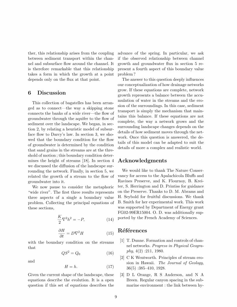
ther, this relationship arises from the couplingbetween sediment transport within the chan-nel and subsurface flow around the channel. Itis therefore remarkable that this relationshiptakes a form in which the growth at a pointdepends only on the flux at that point.

6 Discussion

This collection of bagatelles has been arran-ged as to connect—the way a skipping stoneconnects the banks of a wide river—the flow ofgroundwater through the aquifer to the flow ofsediment over the landscape. We began, in sec-tion 2, by relating a heuristic model of subsur-face flow to Darcy’s law. In section 3, we sho-wed that the boundary condition for the flowof groundwater is determined by the conditionthat sand grains in the streams are at the thre-shold of motion ; this boundary condition deter-mines the height of streams [18]. In section 4we discussed the diffusion of the landscape sur-rounding the network. Finally, in section 5, werelated the growth of a stream to the flow ofgroundwater into it.

We now pause to consider the metaphoric“wide river”. The first three results representsthree aspects of a single a boundary valueproblem. Collecting the principal equations ofthese sections,

K

2∇2h2 = −P, (14)

∂H

∂t= D∇2H (15)

with the boundary condition on the streamsthat

QS2 = Q0 (16)

and

H = h. (17)

Given the current shape of the landscape, theseequations describe the evolution. It is a openquestion if this set of equations describes the

advance of the spring. In particular, we askif the observed relationship between channelgrowth and groundwater flux in section 5 re-present a fourth aspect of this boundary valueproblem ?

The answer to this question deeply influencesour conceptualization of how drainage networksgrow. If these equations are complete, networkgrowth represents a balance between the accu-mulation of water in the streams and the ero-sion of the surroundings. In this case, sedimenttransport is simply the mechanism that main-tains this balance. If these equations are notcomplete, the way a network grows and thesurrounding landscape changes depends on thedetails of how sediment moves through the net-work. Once this question is answered, the de-tails of this model can be adapted to suit thedetails of more a complex and realistic world.

Acknowledgments

We would like to thank The Nature Conser-vancy for access to the Apalachicola Bluffs andRavines Preserve, and K. Flournoy, B. Krei-ter, S. Herrington and D. Printiss for guidanceon the Preserve. Thanks to D. M. Abrams andH. Seybold for fruitful discussions. We thankB. Smith for her experimental work. This workwas supported by Department of Energy grantFG02-99ER15004. O. D. was additionally sup-ported by the French Academy of Sciences.

References

[1] T. Dunne. Formation and controls of chan-nel networks. Progress in Physical Geogra-phy, 4(2) :211, 1980.

[2] C K Wentworth. Principles of stream ero-sion in Hawaii. The Journal of Geology,36(5) :385–410, 1928.

[3] D L Orange, R S Anderson, and N ABreen. Regular canyon spacing in the sub-marine environment : the link between hy-

9

drology and geomorphology. GSA Today,4(2) :35–39, 1994.

[4] S A Schumm, K F Boyd, C G Wolff, andWJ Spitz. A ground-water sapping land-scape in the Florida Panhandle. Geomor-phology, 12(4) :281–297, 1995.

[5] C G Higgins. Drainage systems developedby sapping on Earth and Mars. Geology,10(3) :147, 1982.

[6] D M. Abrams, A E Lobkovsky, A P Pe-troff, K M Straub, B. McElroy, D CMohrig, A. Kudrolli, and D H Rothman.Growth laws for channel networks incisedby groundwater flow. Nature Geoscience,28(4) :193–196, 2009.

[7] J. Bear. Hydraulics of groundwater.McGraw-Hill New York, 1979.

[8] P G Saffman and G I Taylor. The pene-tration of a fluid into a porous medium orHele-Shaw cell containing a more viscousliquid. Proceedings of the Royal Society ofLondon. Series A, Mathematical and Phy-sical Sciences, 245(1242) :312–329, 1958.

[9] M.B. Hastings and L.S. Levitov. La-placian growth as one-dimensional turbu-lence. Physica D : Nonlinear Phenomena,116(1-2) :244–252, 1998.

[10] L. Carleson and N. Makarov. Lapla-cian path models. Journal d’AnalyseMathematique, 87(1) :103–150, 2002.

[11] A.P. Petroff, O. Devauchelle, D.M.Abrams, A.E. Lobkovsky, A. Kudrolli,and D.H. Rothman. Geometry of valleygrowth. Journal of Fluid Mechanics,1(-1) :1–10, 2010.

[12] F. Hecht, O. Pironneau, A. Le Hyaric, andK. Ohtsuka. Freefem++ Manual, 2005.

[13] P G Doyle and J L Snell. Random walksand electric networks. 1984.

[14] A. Sheilds. Anwendungder aehnlichkei ts-mechanik und der turbulenzforschung aufdie geschiebebewegung. Mitteilungen der

Preuss. Versuchsanst fur Wasserbau andSchiffbau, Berlin, 1936.

[15] V.A. Vanoni, WM Keck Laboratory of Hy-draulics, and Water Resources. Measure-ments of critical shear stress for entrainingfine sediments in a boundary layer. Cali-fornia Institute of Technology, 1964.

[16] E. W. Lane. Design of stable channels.Transactions of the American Society ofCivil Engineers, 120 :1234–1260, 1955.

[17] F. M. Henderson. Stability of alluvialchannels. J. Hydraulics Div., ASCE,87 :109–138, 1961.

[18] O. Devauchelle, AP Petroff, AE Lob-kovsky, and DH Rothman. Longitudinalprofile of channels cut by springs. Journalof Fluid Mechanics, 1(-1) :1–11, 2011.

[19] W E H Culling. Analytic theory of erosion.J. Geol., 68 :336–344, 1960.

[20] NW Bass. The geology of cowley county,kansas : Kansas geol. Survey Bull, 12 :1–203, 1929.

[21] KO Emery. Asymmetric valleys of sandiego county, california : Southern calif.acad. Sci. Bull, 46(pt 2) :61–71, 1947.

[22] B.N. Burnett, G.A. Meyer, and L.D. Mc-Fadden. Aspect-related microclimatic in-fluences on slope forms and processes, nor-theastern arizona. Journal of GeophysicalResearch, 113(F3) :F03002, 2008.

[23] E. Istanbulluoglu, O. Yetemen, E.R. Vi-voni, H.A. Gutierrez-Jurado, and R.L.Bras. Eco-geomorphic implications of hil-lslope aspect : inferences from analysisof landscape morphology in central newmexico. Geophysical Research Letters,35(14) :L14403, 2008.

[24] C. Kwit, M.W. Schwartz, W.J. Platt, andJ.P. Geaghan. The distribution of tree spe-cies in steepheads of the apalachicola riverbluffs, florida. Journal of the Torrey Bo-tanical Society, 125(4) :309–318, 1998.

10

[25] I. Reda and A. Andreas. Solar positionalgorithm for solar radiation applications.Solar energy, 76(5) :577–589, 2004.

[26] A E Lobkovsky, B E Smith, A. Kudrolli,D C Mohrig, and D H Rothman. Erosivedynamics of channels incised by subsurfacewater flow. J. Geophys. Res, 112, 2007.

11