Under consideration for publication in J. Fluid Mech. 1

Fountains impinging on a density interface

By JOSEPH K. ANSONG, PATRICK J. KYBAand BRUCE R. SUTHERLAND

Dept. of Mathematical and Statistical Sciences, University of Alberta, Edmonton, AB, CanadaT6G 2G1

(Received 16 April 2007)

We present an experimental study of an axisymmetric turbulent fountain in a two-layerstratified environment. Interacting with the interface, the fountain is observed to exhibitthree regimes of flow. It may penetrate the interface but nonetheless return to the sourcewhere it spreads as a radially propagating gravity current; the return flow may be trappedat the interface where it spreads as a radially propagating intrusion or it may do both.These regimes have been classified using empirically determined regime parameters whichgovern the relative initial momentum of the fountain and the relative density differenceof the fountain and the ambient fluid. The maximum vertical distance travelled by thefountain in a two-layer fluid has been theoretically determined by extending the theorydeveloped for fountains in a homogeneous environment. The theory compares favourablywith experimental measurements. We have also developed a theory to analyse the initialspeeds of the resulting radial currents. The spreading currents exhibited two differentflow regimes: in the constant-velocity regime the initial front position, R, scales withtime, t, as R ∼ t; in the inertia-buoyancy regime, R ∼ t3/4. These regimes were classifiedusing a critical Froude number which characterized the competing effects of momentumand buoyancy in the currents.

1. INTRODUCTION

Turbulent, forced plumes in both homogeneous and stably stratified ambient fluid havereceived considerable attention in part due to their environmental impact in such areas asthe disposal of sewage in the ocean and in lakes, volcanic eruptions into the atmosphereand emissions from chimneys and flares. Recently, the dynamics of plumes and fountainsin enclosed spaces have been studied in order to improve the efficiency through whichrooms are heated and cooled (Lin & Linden (2004)).

Forced plumes are characterized by the competing effects of buoyancy and momentumin the flow. In positively buoyant plumes, the buoyancy and momentum are both inthe same direction with buoyancy becoming more dominant at larger distances awayfrom the source. Negatively buoyant plumes, or fountains, are formed either when densefluid is continuously discharged upward into a less dense fluid or when less dense fluidis injected downward into a more dense environment. In either case, buoyancy opposesthe momentum of the flow until the fountain reaches a height where the vertical velocitygoes to zero. The fountain then reverses direction and falls back upon the source.

Positive and negatively buoyant plumes have been examined theoretically and experi-mentally as they evolve in homogeneous and in linearly stratified environments (Priestley& Ball (1955), Morton (1959b),Turner (1966), Abraham (1963), Fischer et al. (1979), List(1982), Rodi (1982), Bloomfield & Kerr (2000)). Most of this effort was directed at quan-

2 Ansong et. al.

tifying the width of the fountain, the initial and final heights (or penetration depths) andthe entrainment into the fountain.

Fountains in a two-layer stably stratified environment has received relatively littleattention despite its fundamental nature and its potentially practical significance. Aventilated room can naturally form a two layer-stratification and it is of interest to knowhow cold air injected from below mixes in this environment. Jets and fountains in two-layer ambient have also been reported in the situation of refueling compensated fueltanks on naval vessels (Friedman & Katz (2000)). The thermocline in lakes and oceansand atmospheric inversions can be modelled approximately as the interface of a two-layerfluid (Mellor (1996)), and plumes and fountains can result from the release of effluentinto these environments (Rawn et al. (1960), Noutsopoulos & Nanou (1986)).

In particular, this research is motivated in part as the first stage of a program tounderstand the evolution of pollutants from flares that disperse in the presence of anatmospheric inversion. Atmospheric inversions, known for their strong vertical stability,can trap air pollutants below or within them near ground level and so have adverse effectson human health. Hazardous industrial materials that are released into the atmosphereusually form clouds that are heavier than the atmosphere (Britter (1989)). Both Morton(1959a) and Scorer (1959) have applied available mathematical concepts of plume theoryto study the dispersion of pollutants in the atmosphere but ignored the effects of aninversion.

Here we present an experimental study of an axisymmetric fountain impinging on adensity interface in a two-layer stably-stratified environment. As in homogeneous en-vironments, the fountain comes to rest at a maximum height after using up its initialmomentum and then reverses direction interacting with the incident flow.

In a two-layer fluid, however, the reverse flow can either return to the level of thesource or it can become trapped at the density interface. In either case the return flowthen goes on to spread radially outward. We wish to develop a better understandingof the flow through measurements of maximum penetration height, quasi steady-stateheight and radial spreading rate.

There are few experimental studies on fountains in a two-layer environment. Kapoor &Jaluria (1993) considered a two-dimensional fountain in a two-layer thermally stratifiedambient. They provided empirical formulas for the penetration depths in terms of adefined Richardson number.

Some have considered a jet directed into a two-layer ambient with the initial density ofthe jet being the same as the density of the ambient at the source (Shy (1995); Friedman& Katz (2000) and Lin & Linden (2005)). Those jets only become negatively buoyant inthe second layer.

Noutsopoulos & Nanou (1986), studied the upward discharge of a buoyant plume intoa two-layer stratified ambient and used a stratification parameter that depended on thedensity differences in the flow to analyse their results.

One outstanding question concerns whether the reverse flow has a significant effecton the axial velocity and density. By measuring temperatures in a heated turbulentair jet discharged downward into an air environment, Seban et al. (1978) showed thatthe centerline temperatures and the penetration depth can be well predicted by constantproperty theories for the downward flow alone. Mizushina et al. (1982) did a similar studyof fountains by discharging cold water upward into an environment of heated water andfound that the reverse flow had an effect on the axial density measurements.

These experimental results have served only modestly to improve our understanding ofthe dynamics of the reverse flow. A theoretical study aimed at incorporating the reverseflow was first undertaken by McDougall (1981) who developed a set of entrainment

Fountains impinging on a density interface 3

equations quantifying the mixing that occurs in the whole fountain. The ideas developedin the model of McDougall (1981) have recently been built upon by Bloomfield & Kerr(2000) by considering an alternative formulation for the entrainment between the upflowand the downflow. Their results for the width of the whole fountain, the centerline velocityand temperature compared favourably with the experiments of Mizushina et al. (1982).

An important requirement for studying the dispersion of dense gases in the atmo-sphere is a knowledge of the distribution of the concentration as a function of space andtime (Britter (1989)) and how fast the spreading pollutants are moving from a partic-ular location. The usual approach to obtaining information on fluid concentrations inexperiments is by extracting samples from the flow. This is quite difficult and has led tothe introduction of a relatively new approach of laser-induced fluorescence (LIF). Thisis however limited to unstratified environments due to problems with refractive indexfluctuations (Daviero et al. (2001)). In this study, we wish to extract information on theconcentrations of the radial currents using velocity measurements.

In section 2, we review the theory for fountains in a one-layer environment and extend itto the two-layer case. In section 3 we develop the theory for the axisymmetric spreading ofcurrents from fountains. In section 4, we describe the set-up of the laboratory experimentsand the techniques used to visualize the experiments, and we present their qualitativeanalyses. In section 5, quantitative results from the experiments are presented. We analysethe classification of the regimes of flow and compare the measured maximum penetrationheight and spreading velocities to theoretical predictions. In section 6, we summarize theresults.

2. THEORY: PENETRATION HEIGHT

The following theory is developed for fountains in which heavier fluid is injected up-ward into less dense environment. However, in a Boussinesq fluid, for which the densityvariations are small compared with the characteristic density, the direction of motion isimmaterial to the equations governing their dynamics.

2.1. The maximum height in a one-layer ambient

The conventional and most widely used approach to solving problems of turbulent buoy-ant jets is by using the conservation equations of turbulent incompressible flow andemploying the Boussinesq and boundary layer approximations. The resulting equationsare typically solved by using the Eulerian integral method (Turner (1973)). Here a formis first assumed for the velocity and concentration profiles of the plume. This could eitherbe the Gaussian profile or the top-hat profile. The equations are then integrated over theplume cross-section and the assumed profiles are substituted. The result is three ordinarydifferential equations (ODEs) which may be solved analytically or numerically. However,an assumption has to be made to close the system of ODEs. This could either be theentrainment assumption introduced by Morton et al. (1956), or the spreading assumptionintroduced by Abraham (1963).

An alternative approach is the Lagrangian method in which a material volume inthe plume is followed in time (Baines & Chu (1996), Lee & Chu (2003)). The solutionsare much simpler to obtain and interpret and they give very good agreement with theEulerian integral method.

We give a brief review of the Lagrangian method for a fountain in a uniform ambient.Newton’s law is applied to a material volume such that the rate of change of the verticalmomentum of the plume element is equal to the buoyancy force:

4 Ansong et. al.

dM

dt= −Fo, (2.1)

where M and Fo are the momentum and buoyancy flux respectively. Explicitly, assuminga top-hat-shaped plume of radius r and mean vertical velocity w, M = πr2w2 andFo = πr2

owog′, in which g′ = (ρa − ρ)g/ρo is the reduced gravity, ro is the source radius,

wo is the average vertical velocity at the source, ρa is the ambient density, ρ is the densityof the fountain at a given height and ρf is a reference density taken as the initial densityof the fountain. We apply the spreading hypothesis which assumes that dr/dz = β, whereβ is a constant spreading coefficient (β ≈ 0.17 (Baines & Chu (1996))). The buoyancyflux Fo is constant in a uniform ambient. Thus we get the following relations for theradius, r, height, z, volume flux, Q = πr2w, and momentum flux, M , of the fountain asa function of time, t:

r =

(

4β

3√

π

)1/2M

3/4

o

F1/2

o

[

1 −(

1 − Fot

Mo

)3/2]1/2

, (2.2)

z =

(

4

3β√

π

)1/2M

3/4

o

F1/2

o

[

1 −(

1 − Fot

Mo

)3/2]1/2

, (2.3)

Q = M1/2

o

(

4β√

π

3

)

M3/4

o

F1/2

o

(

1 − Fot

Mo

)1/2[

1 −(

1 − Fot

Mo

)3/2]1/2

, (2.4)

M = Mo − Fot, (2.5)

in which Mo = πr2

ow2

o is the momentum flux at the source. At the maximum height themomentum goes to zero, so that from (2.5) we get the time taken to reach the maximumdepth as

tmax =Mo

Fo. (2.6)

Substituting equation (2.6) into (2.3) we get the maximum penetration height of thefountain:

zmax = CfM

3/4

o

F1/2

o

, (2.7)

where Cf =(

4

3β√

π

)1/2

≈ 2.10. This formula was also obtained by Turner (1966) through

dimensional considerations.Equation (2.7) may be rewritten in terms of the source Froude number, Fro=wo/

√g′ro,

such that

zmax = CroFro, (2.8)

in which C =√

8/(3β) ≈ 3.96. As expected, equation (2.4) predicts that the volume fluxdecreases to zero at the maximum height.

Upon reaching the maximum height, the fountain reverses direction interacting withthe incident flow. The interaction between these two opposing fluids inhibits the rise ofthe incident flow to the initial height and so it settles at a quasi steady-state height,

Fountains impinging on a density interface 5

ρo Fo,Qo,Mo

Qi,Mi

Fi

ρ1

ρ2

zvi

H

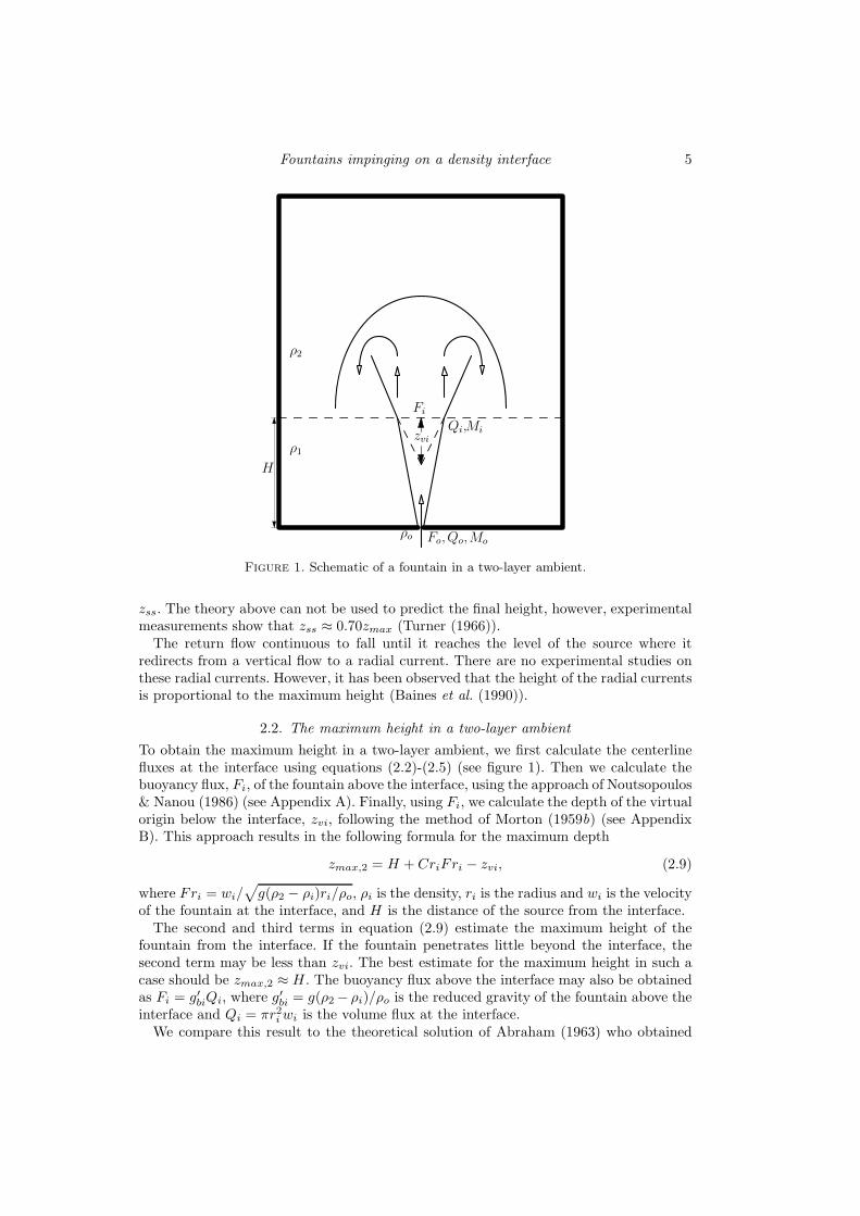
Figure 1. Schematic of a fountain in a two-layer ambient.

zss. The theory above can not be used to predict the final height, however, experimentalmeasurements show that zss ≈ 0.70zmax (Turner (1966)).

The return flow continuous to fall until it reaches the level of the source where itredirects from a vertical flow to a radial current. There are no experimental studies onthese radial currents. However, it has been observed that the height of the radial currentsis proportional to the maximum height (Baines et al. (1990)).

2.2. The maximum height in a two-layer ambient

To obtain the maximum height in a two-layer ambient, we first calculate the centerlinefluxes at the interface using equations (2.2)-(2.5) (see figure 1). Then we calculate thebuoyancy flux, Fi, of the fountain above the interface, using the approach of Noutsopoulos& Nanou (1986) (see Appendix A). Finally, using Fi, we calculate the depth of the virtualorigin below the interface, zvi, following the method of Morton (1959b) (see AppendixB). This approach results in the following formula for the maximum depth

zmax,2 = H + CriFri − zvi, (2.9)

where Fri = wi/√

g(ρ2 − ρi)ri/ρo, ρi is the density, ri is the radius and wi is the velocityof the fountain at the interface, and H is the distance of the source from the interface.

The second and third terms in equation (2.9) estimate the maximum height of thefountain from the interface. If the fountain penetrates little beyond the interface, thesecond term may be less than zvi. The best estimate for the maximum height in such acase should be zmax,2 ≈ H . The buoyancy flux above the interface may also be obtainedas Fi = g′biQi, where g′bi = g(ρ2 − ρi)/ρo is the reduced gravity of the fountain above theinterface and Qi = πr2

i wi is the volume flux at the interface.We compare this result to the theoretical solution of Abraham (1963) who obtained

6 Ansong et. al.

the following approximate analytic solution for the penetration of a turbulent buoyantjet moving into an environment consisting of a series of layers of different densities:

zmax,2 =

(

2

5

)1/6 (

3

2− µF̃

)1/2

H, (2.10)

in which F̃ = w2

i /((ρi−ρ2)gH/ρo) and the empirical constant µ ≈ 0.8 (Abraham (1963)).This derivation was done by assuming Gaussian profiles of the flow quantities unlike thetop-hat approach considered in this study.

Similar to the one-layer case, the interaction of the incident and reverse flows inhibitsthe incident flow from reaching the maximum height and thus settles at a quasi steady-state height, zss,2. Unlike the one-layer case, the return flow may intrude on the interfaceor continue to the level of the source. Our experiments show that the ratio of the steady-state height to the maximum height depends on whether the return flow went back tothe source or collapsed at the interface (see section 5.2).

The most significant factors governing these flow regimes are the relative density differ-ences between the two layer and fountain and the maximum height relative to the height,H , of the layer at the source. Explicitly, the relative density differences are characterizedby

θ =

∣

∣

∣

∣

ρ2 − ρ1

ρ2 − ρo

∣

∣

∣

∣

, (2.11)

and the relative maximum height is characterized by zmax/H .θ = 0 if ρ2 = ρ1, in which case the ambient is a one-layer fluid and the fountain must

return to the source. The same circumstance is expected if zmax < H since the fountaindoes not reach the position of the interface.

θ = 1 if ρ1 = ρo, in which case the flow does not act like a fountain until impacting thesecond layer. No experiments were conducted for this case, but the interested reader mayrefer to the studies by Shy (1995), Friedman & Katz (2000) and Lin & Linden (2005).Given that the jet penetrates the interface (zmax > H), the resulting fountain will beexpected to return to spread along the interface since the fountain entrains less densefluid from beyond the interface and therefore becomes lighter than the ambient fluid atthe source.

Irrespective of the regime that occurs, the flow goes on to spread as a radial current.

3. THEORY: SPREADING VELOCITIES

In the following, we derive a theory to analyse the velocities of the spreading currentsat the source and the interfacial intrusions. We consider only the radial velocities at theradius of the whole fountain where the return flow redirects from a vertical to a horizontalflow.

There are three cases to be considered. We first consider the theory for the spreadingvelocities of the currents at the source in the one-layer case and then extend it to examinesource-spreading of fountains in two-layer fluids. The velocities of radial intrusions at theinterface of a two-layer fluid is considered as a third case.

3.1. Case 1: one-layer source-spreading

Figure 2a is a schematic showing the spreading of the currents at the source from afountain in a one-layer environment. Baines et al. (1990) modelled the return flow of aturbulent fountain as an annular plane plume and obtained a formula for the total lateral

Fountains impinging on a density interface 7

FoQo,Mo, Rf

vfh

Qe

(a)ρoFoQo,Mo,

vfh

H ρ1

ρ2

Qe

(b)

Figure 2. Schematics of (a) one-layer surface spreading currents, and (b) a model of theinterfacial spreading currents.

entrainment into the reverse flow as

Qe = B(zmax − zv)

roQo, (3.1)

where B ≈ 0.25 was obtained as an experimental constant and zv is the distance of thevirtual origin below the source (zv ≈ 0.8 cm for our experiments). Thus, the total volumeflux at the level of the source, just as the flow begins to spread outward is given by

QT = Qe + Qo. (3.2)

If vf is the initial spreading velocity at a radial distance Rf , where Rf is the radius ofthe return flow at the source, and h is the height of the spreading layer, then

QT = 2πRfhvf . (3.3)

Defining g′T = g(ρ1 − ρs)/ρo to be the reduced gravity and ρs to be the initial density ofthe spreading layer at r = Rf , dimensional analysis gives, for a buoyancy-driven flow, arelationship of the form vf ∝

√

g′T h. Using (3.3) we get

vf ∝(

QT g′TRf

)1/3

. (3.4)

Mizushina et al. (1982) show that the radius of the whole fountain is approximatelyconstant and is about 22% of the quasi-steady state height, zss. Just before the returnflow begins to spread into the ambient, conservation of buoyancy flux in the fountainrequires that at the level of the source

QT g′T = Fo. (3.5)

Thus, from (3.4) and (3.5) we get

vf ∝(

Fo

Rf

)1/3

∝(

Fo

zss

)1/3

. (3.6)

8 Ansong et. al.

This formula may also be obtained via scaling analysis. By balancing the drivingbuoyancy force which scales as g′T ρsRh2, and the retarding inertia force which scales asρshR3/t2, Chen (1980) obtained the position of the front, R, as a function of time, t, as

R(t) = cF1/4

o t3/4 (where c = 0.84 was obtained as an experimental constant), thus thevelocity, v, is given by

v =dR

dt= 0.59

(

Fo

R

)1/3

, (3.7)

where the global volume conservation relation, QT t = πR2h, has been employed.

The scaling relationships above assume that the flow is a pure gravity current, itsmotion being dominated by buoyancy forces. In the presence of substantial radial mo-mentum at the point where the flow enters the environment, dimensional analysis showsthat at small times compared with the characteristic time scale tMF = MR/FR (in whichMR is the radial component of momentum flux and FR is the radial buoyancy flux), the

flow is dominated by momentum such that R(t) ∼ M1/4

R t1/2 (Chen (1980)), so that

v ∼ (M1/2

R /R). (3.8)

The recent study by Kotsovinos (2000) for constant-flux axisymmetric intrusions into alinearly stratified ambient revealed a constant-velocity regime where R ∼ t. Kotsovinos(2000) argued that the additional force driving the flow in such cases is the initial radialmomentum flux (ρsMR). This corresponds to times when both momentum and buoyancyare comparable in the flow (t ≈ tMF ). Thus, balancing the kinematic momentum fluxand the inertia force which scales as ρshR3/t2, gives R(t) ∼ (MR/QT )t, so that

v ∼ (MR/QT ). (3.9)

In theory, the relations in equations (3.6) and (3.7) correspond to larger times within theinertia-buoyancy regime when the flow is purely driven by buoyancy.

The radial component of momentum is unknown a priori ; however, due to the loss inmomentum by moving from a vertical flow to a radial current, we assume that the initialradial momentum flux, MR, is proportional to the momentum flux of the return flow atthe level of the source, Mret, and defined as

Mret = π(R2

f − r2

o)w2

ret, (3.10)

where wret is the velocity of the return flow at the level of the source. The results ofBloomfield & Kerr (2000) show that the reverse flow of the fountain moving back towardthe source first accelerates to some height before settling to an almost constant velocityclose to the source. Their results also suggest that at the source, the velocity of the returnflow is such that

wret ∝ M−1/4

o F 1/2

o . (3.11)

In summary, if the radial momentum of the initial flow is substantial, then three regimesare theoretically possible. These are the radial-jet regime where R ∼ t1/2, the constant-velocity regime where R ∼ t and the inertia-buoyancy regime where R ∼ t3/4. Thus,from (3.8), (3.9) and (3.6), and replacing MR by Mret, we get the following relationswhich may be used to predict the initial velocity of the spreading currents just as the

Fountains impinging on a density interface 9

flow begins to spread into the ambient:

vt<<tMF∝ (M

1/2

ret /zss), (3.12)

vt≈tMF∝ (Mret/QT ), (3.13)

vt>>tMF∝ (Fo/zss)

1/3. (3.14)

However not all three regimes are necessarily present in a single experiment; the pres-ence of a particular regime largely depends on the competing effects of the radial com-ponents of momentum and buoyancy in the flow (Chen (1980), Kotsovinos (2000)).

3.2. Case 2: two-layer surface-spreading

We consider the case where the return flow in the two-layer case returns to spread at thesource as an axisymmetric current. In this case, there are two buoyancy fluxes involvedin the system: the initial buoyancy flux, Fo, and the buoyancy flux after the fountainpenetrates the density interface, Fi. At the level of the source, we require that the sumof these fluxes remain conserved in the fountain so that

QT g′T = Fo + Fi. (3.15)

Thus, we get the spreading velocity from equation (3.4) as

vt>>tMF∝

(

Fo + Fi

zss,2

)1/3

(3.16)

where zss,2 is the steady-state height in the two-layer case.We assume that the velocity and momentum of the return flow at the level of the

source are proportional to the corresponding velocity and momentum in the one-layercase where the ambient fluid is the first layer fluid. As such, if the initial radial momentumflux is substantial, then equations (3.12) and (3.13) may still be applied. By replacingMR with Mret, this argument results in the velocity relations for the radial-jet andconstant-velocity regimes respectively as

vt<<tMF∝ (M

1/2

ret /zss,2), (3.17)

vt≈tMF∝ (Mret/QT ). (3.18)

3.3. Case 3: two-layer interfacial-spreading

Experiments on axisymmetric intrusions into two-layer ambients from a source of con-stant volume flux are limited in the literature. Lister & Kerr (1989) have consideredthe case of the spreading of highly viscous fluid into a two-layer environment. They em-ployed both scaling analysis and lubrication theory to analyse their results. Timothy(1977) considered the general case of a stratified inflow into a stratified ambient andtreated the two-layer case as a special circumstance. Most of his results were derived byextending the Bernoulli and hydrostatic equations for two-dimensional rectilinear flowsto axisymmetric flows.

We show in Appendix C that by balancing the horizontal driving buoyancy force andthe retarding inertia force, for a buoyancy-driven flow, we obtain the relation for theradial velocity of the intrusion as

v ∝(

εg′T QT

R

)1/3

, (3.19)

where ε = (ρ2−ρs)/(ρ2−ρ1). The reduced gravity of the intrusion in this case is modified

10 Ansong et. al.

by the parameter ε. Given that the density of the intrusion is equal to the density of thefirst layer fluid (ρs = ρ1), then the one-layer relation (3.7) is retrieved from (3.19).

To model the case of the intrusions, we consider the fountain beyond the interface asthough it is a one-layer system with the source conditions replaced by the conditions atthe interface (see figure 2b). We therefore assume the conservation of buoyancy relationεg′T QT = Fo + Fi, and get the same proportionality relationship as in (3.16) althoughthe proportionality constant is different:

vt>>tMF∝

(

Fo + Fi

Rf

)1/3

∝(

Fo + Fi

zss,2

)1/3

. (3.20)

In the presence of a substantial radial component of momentum, equations (3.12) and(3.13) may be applied with the initial source conditions replaced by the conditions at theinterface. This gives the velocity formulas for the radial-jet and constant-velocity regimesrespectively as

vt<<tMF∝ M

1/2

ret,i/zss,2, (3.21)

vt≈tMF∝ Mret,i/QT , (3.22)

where Mret,i is the vertical momentum of the return flow at the interface and defined as

Mret,i = π(R2

f − r2

i )w2

ret,i with wret,i ∝ M−1/4

i F1/2

i , where wret,i is the velocity of thereturn flow at the interface.

4. EXPERIMENTAL SET-UP AND ANALYSES

4.1. Experimental set-up

Experiments are performed in an acrylic tank measuring 39.5 cm long by 39.5 cm wide by39.5 cm high (see figure 3). The experiments were conducted by injecting less dense fluiddownward into more dense ambient fluid, however, the direction of motion is immaterialto the equations governing their dynamics since the fluid is considered to be Boussinesq.A control experiment was conducted in a one-layer homogeneous environment and 48experiments were conducted in two-layer fluid. In all experiments, the total depth offluid within the tank was HT = 38 cm. The tank was filled to a depth of HT − H withfluid of density ρ2, where H = 0 in the case of one-layer experiments and H = 5 cm or10 cm in two-layer experiments. In two-layer experiments, a layer of water with densityρ1 was added through a sponge float until the total depth was HT . The typical interfacethickness between the two layers was 1 cm, sufficiently small to be considered negligible.

After the one or two-layer fluid in the tank was established, a constant-head reservoirof fresh water of density ρo was dyed with a blue food colouring and then allowed todrain into the tank through a round nozzle of radius 0.2 cm. To ensure the flow turbu-lently leaves the nozzle, the nozzle was specially designed and fitted with a mesh havingopenings of extent 0.05 cm. The flow was assumed to leave at a uniform velocity acrossthe diameter of the nozzle. The flow rates for the experiments were recorded using a flowmeter connected to a plastic tubing, and by measuring the total volume released duringan experiment. Flow rates ranged from 2.82 to 3.35 cm3/s.

Experiments were recorded using a digital camera situated 250 cm from the front ofthe tank. The camera was situated at a level parallel to the mid-depth of the tank andthe entire tank was in its field of view. A lighting apparatus was also placed about 10 cmbehind the tank to illuminate the system.

Using “DigImage” software, the maximum penetration depth of the fountain, the quasi

Fountains impinging on a density interface 11

H

HT

ρ1

ρ2

ρ0

nozzle

connecting tube

tank

39.5 cm

Figure 3. Experimental set-up and definition of parameters.

steady-state depth and the initial velocity, wo, were determined by taking vertical time-series constructed from vertical slices through the nozzle. The temporal resolution wasas small as 1/30 s and the spatial resolution was about 0.1 cm.

Horizontal time series were used to determine the velocity of the resulting spreadingcurrents. They were taken at a position immediately below the nozzle. Most time seriesare symmetrical about the position of the nozzle and only one side is used for the calcu-lation of the velocities. Asymmetry in the time series may arise due to instabilities in theflow causing the front of the fountain at the maximum depth to tilt to one side. Theseexperiments were excluded from the analyses.

4.2. Qualitative results

We present in this section the qualitative results of the laboratory experiments beforegiving detailed analyses of them. The snapshots from the experiments are flipped up-side down for conceptual convenience and for consistency with the theory. We will firstdescribe the results of the one-layer experiment before proceeding to the two-layer case.

4.2.1. One-layer experiment

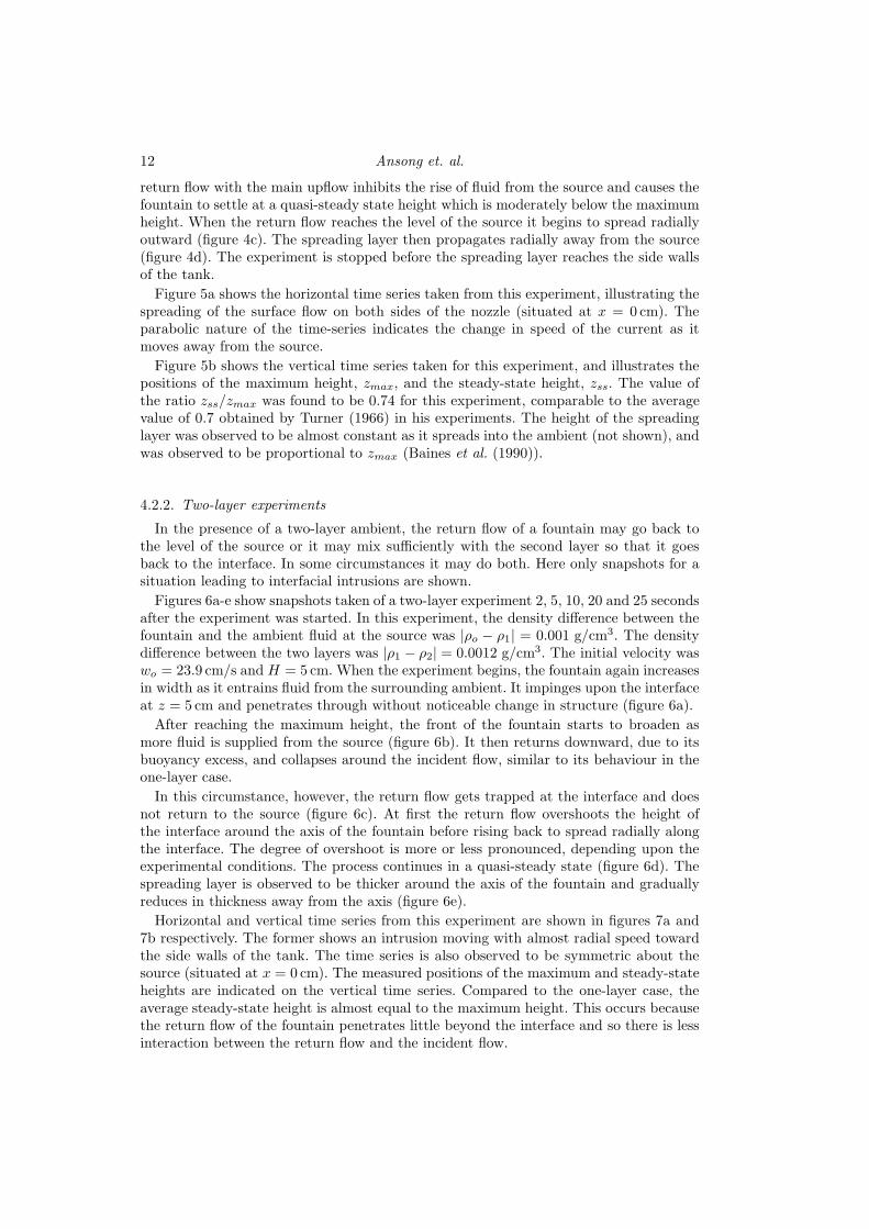
Figures 4a-d show snapshots of the one-layer experiment which were taken 1, 3, 5, and8 seconds, respectively, after the experiment started. The density difference between thefountain and the ambient fluid was |ρo − ρ1| = 0.0242 g/cm3 and the initial velocity waswo = 24.3 cm/s. We observe the characteristic widening of the fountain as it entrains fluidfrom the surrounding homogeneous fluid. It reaches its maximum height at t ∼ 1 s (figure4a), at which time the top of the fountain forms a pointed shape before collapsing backtoward the source. The front then broadens and spreads outward as it returns downwardforming a curtain around the incident upward flow (figure 4b). The interaction of the

12 Ansong et. al.

return flow with the main upflow inhibits the rise of fluid from the source and causes thefountain to settle at a quasi-steady state height which is moderately below the maximumheight. When the return flow reaches the level of the source it begins to spread radiallyoutward (figure 4c). The spreading layer then propagates radially away from the source(figure 4d). The experiment is stopped before the spreading layer reaches the side wallsof the tank.

Figure 5a shows the horizontal time series taken from this experiment, illustrating thespreading of the surface flow on both sides of the nozzle (situated at x = 0 cm). Theparabolic nature of the time-series indicates the change in speed of the current as itmoves away from the source.

Figure 5b shows the vertical time series taken for this experiment, and illustrates thepositions of the maximum height, zmax, and the steady-state height, zss. The value ofthe ratio zss/zmax was found to be 0.74 for this experiment, comparable to the averagevalue of 0.7 obtained by Turner (1966) in his experiments. The height of the spreadinglayer was observed to be almost constant as it spreads into the ambient (not shown), andwas observed to be proportional to zmax (Baines et al. (1990)).

4.2.2. Two-layer experiments

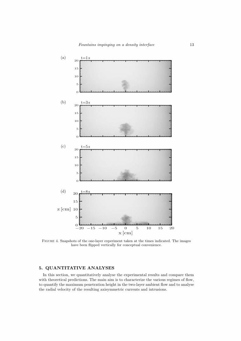
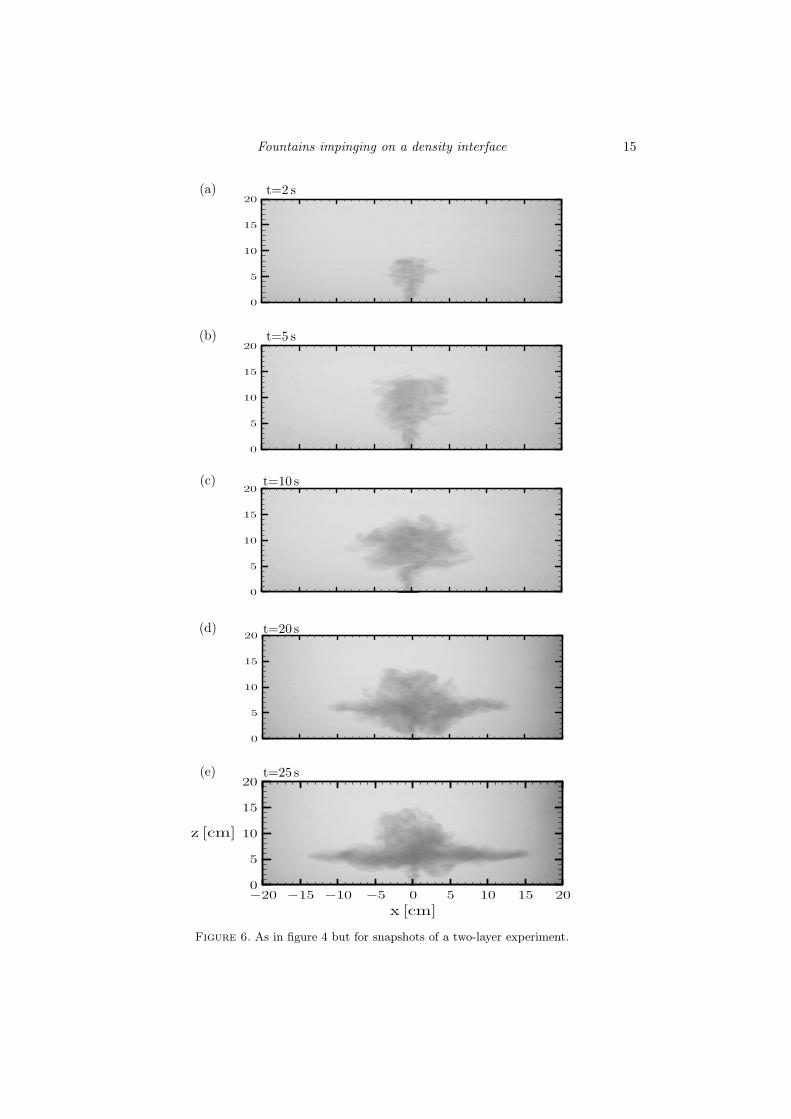
In the presence of a two-layer ambient, the return flow of a fountain may go back tothe level of the source or it may mix sufficiently with the second layer so that it goesback to the interface. In some circumstances it may do both. Here only snapshots for asituation leading to interfacial intrusions are shown.

Figures 6a-e show snapshots taken of a two-layer experiment 2, 5, 10, 20 and 25 secondsafter the experiment was started. In this experiment, the density difference between thefountain and the ambient fluid at the source was |ρo − ρ1| = 0.001 g/cm3. The densitydifference between the two layers was |ρ1 − ρ2| = 0.0012 g/cm3. The initial velocity waswo = 23.9 cm/s and H = 5 cm. When the experiment begins, the fountain again increasesin width as it entrains fluid from the surrounding ambient. It impinges upon the interfaceat z = 5 cm and penetrates through without noticeable change in structure (figure 6a).

After reaching the maximum height, the front of the fountain starts to broaden asmore fluid is supplied from the source (figure 6b). It then returns downward, due to itsbuoyancy excess, and collapses around the incident flow, similar to its behaviour in theone-layer case.

In this circumstance, however, the return flow gets trapped at the interface and doesnot return to the source (figure 6c). At first the return flow overshoots the height ofthe interface around the axis of the fountain before rising back to spread radially alongthe interface. The degree of overshoot is more or less pronounced, depending upon theexperimental conditions. The process continues in a quasi-steady state (figure 6d). Thespreading layer is observed to be thicker around the axis of the fountain and graduallyreduces in thickness away from the axis (figure 6e).

Horizontal and vertical time series from this experiment are shown in figures 7a and7b respectively. The former shows an intrusion moving with almost radial speed towardthe side walls of the tank. The time series is also observed to be symmetric about thesource (situated at x = 0 cm). The measured positions of the maximum and steady-stateheights are indicated on the vertical time series. Compared to the one-layer case, theaverage steady-state height is almost equal to the maximum height. This occurs becausethe return flow of the fountain penetrates little beyond the interface and so there is lessinteraction between the return flow and the incident flow.

Fountains impinging on a density interface 13

0

5

10

15

20t=1 s(a)

0

5

10

15

20t=3 s(b)

0

5

10

15

20t=5 s(c)

0

5

10

15

20

z [cm]

−20 −15 −10 −5 0 5 10 15 20

x [cm]

t=8 s(d)

Figure 4. Snapshots of the one-layer experiment taken at the times indicated. The imageshave been flipped vertically for conceptual convenience.

5. QUANTITATIVE ANALYSES

In this section, we quantitatively analyse the experimental results and compare themwith theoretical predictions. The main aim is to characterize the various regimes of flow,to quantify the maximum penetration height in the two-layer ambient flow and to analysethe radial velocity of the resulting axisymmetric currents and intrusions.

14 Ansong et. al.

0

5

10

15

20

t [s]

−20 −10 0 10 20

x [cm]

(a)

0

5

10

15

z [cm]

0 2 4 6 8

t [s]

(b)

zmax

zss

Figure 5. (a) Horizontal and (b) vertical time series for a 1-layer experiment. The horizontaltime series is constructed from a slice taken at z = 0 cm. The vertical time series is taken froma vertical slice through the source at x = 0 cm.

5.1. Regime Characterization

The three regimes of flow observed in the experiments: in regime S, the return flowpenetrates the interface but returns vertically to the source; in regime I, the return flowintrudes at the interface; in regime B, a combination of both occurs.

Figure 8 shows a plot of the relative density differences θ = (ρ2−ρ1)/(ρ2−ρo) againstthe relative maximum height zmax/H .

If θ & 0.15, figure 8 shows that intrusions form if zmax & 2H . In which case the returnflow entrains substantially less dense fluid from beyond the interface, greatly reducingits buoyancy excess.

If θ . 0.15, the return flow reaches the source independent of the relative maximumheight. In this case the return flow entrains less dense fluid from beyond the interface butthe buoyancy excess of the fountain is not substantially reduced. Likewise if zmax . 2Hthe return flow always reaches the source because it is not sufficiently diluted by theambient beyond the interface.

There were two experiments which resulted in regime B. They occurred for experimentswith zmax ≈ 2H . In these cases, the outer part of the return flow entrains more of theless dense fluid from beyond the interface than the inner part. The lighter outer partthen begins to spread radially at the interface while the heavier inner part continues tofall to the source. The amount of fluid that intrudes at the interface may sometimes besmaller than the fluid that continues to the source.

The empirical function used to separate the intrusion and source outflow regimes is

Fountains impinging on a density interface 15

0

5

10

15

20t=2 s(a)

0

5

10

15

20t=5 s(b)

0

5

10

15

20t=10 s(c)

0

5

10

15

20t=20 s(d)

0

5

10

15

20

z [cm]

−20 −15 −10 −5 0 5 10 15 20

x [cm]

t=25 s(e)

Figure 6. As in figure 4 but for snapshots of a two-layer experiment.

16 Ansong et. al.

0

5

10

15

20

t [s]

−20 −10 0 10 20

x [cm]

(a)

0

5

10

15

z [cm]

0 5 10 15 20

t [s]

(b)

zmax z

ss

Figure 7. (a) As in figure 5 but for horizontal and (b) vertical time series for a 2-layerexperiment.

given by

θ = 0.15 +1

50(zmax/H − 1.5)3. (5.1)

This is plotted as the dashed line in figure 8.

5.2. Maximum height

Figure 9a plots the experimentally measured values of zmax,2 and compares them with thetheoretical prediction given by equation (2.9). There is good agreement in the data witha correlation of about 96%. The results also compare well with the theoretical predictionof Abraham (1963) (see equation (2.10)).

Figure 9b plots the ratio zss,2/zmax,2 against the source Froude number Fro. If θ < 0.15,the average value of the ratio was found to be 0.74, which is comparable to the one-layercase. For the experiments with θ > 0.15 and zmax > 2H in which case the return flowintruded on the interface, the average value was 0.88. This occurs because the returnflow penetrates little beyond the interface and so there is less interaction between thereturn and incident flows. If θ > 0.15 and zmax < 2H , the average value was found to be0.80, in this case the fountain penetrated little into the second layer and the steady-stateheight was found to be closer to the maximum height.

5.3. Radial source and intrusion speeds

We measured the initial velocity of the radially spreading currents by taking the slopenear x ≈ Rf of horizontal time series as shown, for example, in figure 10.

Fountains impinging on a density interface 17

0 2 4 6 80

0.1

0.2

0.3

0.4

0.5

0.6

0.7

0.8

0.9

1

θ

zmax

/H

Source, H=5 cmSource, H=10 cmInterface, H=5 cmInterface, H=10 cmBoth, H=5 cm

Figure 8. Regime diagram showing circumstances under which the return flow of a fountainspreads at the level of the source (open symbols), at the interface (closed symbols) or both.The dotted line represents an empirical formula that separates the two regimes and given byequation (5.1).

Measurements of the time and distance from the horizontal time series determined howthe position of the front scales with time near x = Rf . Figure 11 shows some typicallog-log plots of distance against time used to determine the scaling relationship. Theexperiments showed steady state (R ∼ t) and inertia-buoyancy (R ∼ t3/4) regimes in theflow.

To gain a better understanding of the starting flow regimes, we defined a critical Froudenumber to characterize the competing effects of momentum and buoyancy in the returnflow at the point of entry of the current into the ambient. In the case of the flows thatreturned to the source, the Froude number is defined by

Frs = wret/(g′retzmax,2)1/2, (5.2)

where g′ret = (Fo + Fi)/QT is the reduced gravity of the return flow at the level of thesource. In the case of the interfacial flows, the Froude number is similarly defined by

Fri = wret,i/(g′ret,izmax,2)1/2, (5.3)

where g′reti is the reduced gravity of the return flow at the interface. Figure (12) gives anapproximate classification of these regimes. It shows that the power law relation R ∼ tα

with α ≈ 0.75 occurs for smaller values of the Froude number (Frs < 0.25 and Fri < 0.4).In this case, the initial flow is purely driven by buoyancy forces while for larger valuesof the Froude number (Frs > 0.25 and Fri > 0.4), both momentum and buoyancy arecomparable in the initial flow, giving rise to a power law exponent α ≈ 1.0.

If instabilities develop in the flow to cause the fountain to tilt initially to one side ofits vertical axis, then these scaling relationships may be violated. This was also observedto occur if, in the case of the intrusions, there was a very strong overshoot of the return

18 Ansong et. al.

0 5 10 15 20 25 300

5

10

15

20

25

30

zmax,2

(theory)

zm

ax

,2(e

xp

eri

me

nt)

This studyAbraham(1963)SourceInterfaceBoth

(a)

0 10 20 30 40 500

0.1

0.2

0.3

0.4

0.5

0.6

0.7

0.8

0.9

1

Fro=w

o/(r

og,)1/2

zs

s,2

/zm

ax

,2

Source ( θ<0.15 )Source ( θ>0.15 )InterfaceBoth

(b)

Figure 9. (a) The maximum penetration height and (b) the ratio of the steady-state height tothe maximum height

flow before rising back to spread along the interface. The velocity data that was used todetermine the experimental constants in the theory does not include those experiments.

5.3.1. Source-spreading speeds

Figures 13a and 13b plots the measured speeds of the radially propagating currents atthe source compared with the theoretical estimates of equations (3.16) and (3.18). Wesee that there is fairly good agreement between the theory and the measurement. Thetheoretical equations for these two regimes then become

vt≈tMF= (4.10 ± 0.14)

(

Mret

QT

)

, (5.4)

and

vt>>tMF= (0.84 ± 0.14)

(

Fo + Fi

zss,2

)1/3

. (5.5)

The regimes of flow in this case are the constant-velocity regime (R ∼ tα with α =1.0 ± 0.10) and the inertia-buoyancy regime (α = 0.75 ± 0.04).

5.3.2. Intrusion speeds

Figure 14 plots the measured intrusion speeds against the theoretical estimates ofequations (3.20) and (3.22). The theoretical equations for these two regimes then become

vt≈tMF= (0.77 ± 0.15)

(

Mreti

QT

)

, (5.6)

and

vt>>tMF= (0.17 ± 0.09)

(

Fo + Fi

zss,2

)1/3

. (5.7)

Fountains impinging on a density interface 19

0 5 10 15 200

5

10

15

20

25

x

t

∆ x∆ t

^x=Rf

experimental datafitted line

Figure 10. Typical approach of calculating the initial spreading speeds with ∆x ≈ Rf

(experiment with |ρ1 − ρo| = 0.0202, |ρ2 − ρ1| = 0.0005, H = 5 cm, wo = 26.26 cm/s).

100

101

10210

0

101

102

log t

log

R

R = 0.97 t1.01

experimental datafitted line

(a)

100

101

102

log t

R = 1.02 t0.78

experimental datafitted line

(b)

Figure 11. Typical initial growth relationships between the radial distance and time, indicating(a) R ∼ t (experiment with |ρ1 − ρo| = 0.0022, |ρ2 − ρ1| = 0.005, H = 5 cm, wo = 25.95 cm/s),

and (b) R ∼ t3/4 (experiment with |ρ1 − ρo| = 0.0202, |ρ2 − ρ1| = 0.0005, H = 5 cm, andwo = 26.26 cm/s)

The regimes of flow in this case are the constant-velocity regime (α = 1.0 ± 0.09) andthe inertia-buoyancy regime (α = 0.75 ± 0.07).

We observe that the proportionality constants in the interfacial intrusions are muchsmaller than the constants in the source-spreading case. This is probably caused byhigher retarding forces exerted by the two fluid layers on the interfacial currents unlikethe currents at the source which propagate on the interface between air and liquid andtherefore experienced a much smaller resisting force from the ambient.

20 Ansong et. al.

0 0.1 0.2 0.3 0.4 0.50.5

0.6

0.7

0.8

0.9

1

1.1

1.2

1.3

Frs=w

ret/(g’

retzmax,2)1/2

α

(a)

0.2 0.25 0.3 0.35 0.4 0.45 0.5 0.550.5

0.6

0.7

0.8

0.9

1

1.1

1.2

1.3

Fri=w

reti/(g’

retizmax,2)1/2

α

(b)

Figure 12. Characterizing the initial power law behaviour, R ∼ tα, using a defined radialFroude number for the (a) surface flows, and (b) interfacial flows. The open diamond (♦) refersto α ≈ 0.75 and the closed circles (•) refers to α ≈ 1. Typical errors are indicated in the top leftcorner of both plots.

0 0.1 0.2 0.3 0.40

0.5

1

1.5

Vt≈ t

MF

=(Mret

/QT) [cm/s]

VE

xp

eri

men

t[cm

/s]

(a)

0 0.4 0.8 1.2 1.60

0.4

0.8

1.2

1.6

Vt>>t

MF

= [(Fo+F

i)/z

ss]1/3 [cm/s]

VE

xp

eri

men

t [c

m/s

]

(b)

Figure 13. Radial initial surface spreading velocities for (a) R ∼ t, and (b) R ∼ t3/4

6. Summary and conclusions

We have classified the regimes of flow that result when the return flow of an axisym-metric turbulent fountain is discharged into a two-layer ambient. The classification wasdone using the empirically determined parameter, θ = (ρ2 − ρ1)/(ρ2 − ρo), and the rela-tive maximum height, zmax/H . The results show that if zmax . 2H , the return flow willgo back to the source irrespective of the value of θ. However, if zmax & 2H , the returnflow will collapse and spread radially at the interface if θ & 0.15.

We found good agreement between theory and experiment for the maximum vertical

Fountains impinging on a density interface 21

0 0.5 1 1.50

0.4

0.8

1.2

Vt≈ t

MF

=(Mret,i

/QT) [cm/s]

VE

xp

eri

men

t [c

m/s

]

(a)

0 1 2 3 4 5 6 70

0.2

0.4

0.6

0.8

1

1.2

Vt>>t

MF

= [(Fo+F

i)/z

ss]1/3[cm/s]

VE

xp

eri

men

t [c

m/s

]

(b)

Figure 14. Radial initial intrusion velocities for (a) R ∼ t, and (b) R ∼ t3/4

penetration height. In the case of flows which returned to the source, the ratio of thequasi-steady state height to the maximum height, zss,2/zmax,2, was found to depend onwhether the return flow went back to the source or collapsed at the interface. The ratio iscloser to unity (zss,2/zmax,2 ≈ 1.0) for intrusions because the return flow does not retardthe incident flow in the ambient near the source.

Radial currents that result from the return flow of a fountain spreading at the sourceor interface either at constant-velocity (being driven by both the radial components ofmomentum and buoyancy) or spreading as R ∼ t3/4 (being driven by buoyancy forcesalone). These regimes are distinguished by a critical Froude number Frs ≈ 0.25 or Fri ≈0.4.

In the future, we wish to extend the ideas developed in this study to the case of thedispersion of pollutants from flares which disperse in the presence of an atmosphericinversion.

This research was supported by the Canadian Foundation for Climate and AtmosphericScience (CFCAS).

Appendix A. Buoyancy flux above the interface

Noutsopoulos & Nanou (1986) obtained the nominal value of the buoyancy flux, Fi,above the interface:

Fi =1

ρo

∫

A

g(ρ2 − ρ)wdA = g(ρ1 − ρo)

ρoQo − g

(ρ1 − ρ2)

ρoQi = Fo

[

1 − ε̃Qi

Qo

]

,

where Qi is the volume flux at the interface and ε̃ = (ρ1 − ρ2)/(ρ1 − ρo).

Appendix B. Virtual origin correction

Morton (1959b) predicted the virtual origin for a negatively buoyant forced plume tooccur at

22 Ansong et. al.

zv = 101/2γ3/2Lm

∫

1

1/γ

(1 − τ5)−1/2τ3dt, (B 1)

where

Lm =1

(

23/2α̃1/2π1/4λ)

M3/4

o

|Fo|1/2, Γ =

5λ2

4α̃π1/2

|Fo|Q2o

M5/2

o

and γ = (1 − Γ)1/5.

The entrainment constant is α̃ = 0.085 for fountains (Bloomfield & Kerr (2000)) andλ = 1 for top-hat profiles.

Appendix C. Scaling Analyses: Radial intrusion in a two-layer

environment

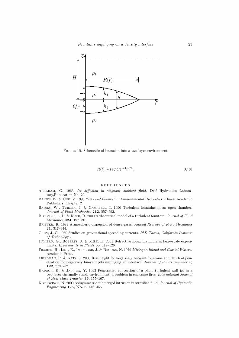
Consider an axisymmetric intrusion of density ρs from a source of constant volumeflux QT into a two-layer environment with a top layer of density ρ1 and a lower layerof density ρ2. Let h be the height of the intrusion at time t and H be the distance ofthe interface from the surface as shown in figure 15. We assume small density differencesbetween the intrusion and the ambient and neglect surface tension effects.

The conservation of volume relation is given by

QT t ∼ R2h, (C 1)

where R is the position of the front at time t. The pressure distribution within theintrusion can be obtain from the hydrostatic equation (dp/dz = −ρsg) such that

p = po − ρsgz + g(ρs − ρ1)h1 (C 2)

where po = ρ1gH . A relation between h1 and h is obtained via a hydrostatic balance(Timothy (1977)):

h1 =

(

ρ2 − ρs

ρ2 − ρ1

)

h. (C 3)

Thus, from equation (C 2) we get the pressure distribution

p = po − ρsgz + ρsεg′h (C 4)

where ε = (ρ2 − ρs)/(ρ2 − ρ1) and g′ = g(ρs − ρ1)/ρs. The radial pressure gradient istherefore given by

∂p

∂r= ρsεg

′ ∂h

∂r. (C 5)

At the interface, z = 0, the pressure scales as p ∼ ρsεg′h and so the horizontal driving

pressure force should scale as the product of the pressure and the cross-sectional area:

Fp ∼ ρsεg′Rh2. (C 6)

In the inertia-buoyancy regime, the opposing force is the inertia force, Fin, which scalesas the product of the mass and volume:

Fin ∼ ρshR3/t2. (C 7)

Balancing equations (C 6) and (C 7) and using equation (C 1), we get

Fountains impinging on a density interface 23

r

z

R(t)

h1

h2

h

Hρ1

ρs

ρ2

QT

Figure 15. Schematic of intrusion into a two-layer environment

R(t) ∼ (εg′Q)1/4t3/4. (C 8)

REFERENCES

Abraham, G. 1963 Jet diffusion in stagnant ambient fluid . Delf Hydraulics Labora-tory,Publication No. 29.

Baines, W. & Chu, V. 1996 “Jets and Plumes” in Environmental Hydraulics. Kluwer AcademicPublishers, Chapter 2.

Baines, W., Turner, J. & Campbell, I. 1990 Turbulent fountains in an open chamber.Journal of Fluid Mechanics 212, 557–592.

Bloomfield, L. & Kerr, R. 2000 A theoretical model of a turbulent fountain. Journal of FluidMechanics 424, 197–216.

Britter, R. 1989 Atmospheric dispersion of dense gases. Annual Reviews of Fluid Mechanics21, 317–344.

Chen, J.-C. 1980 Studies on gravitational spreading currents. PhD Thesis, California Instituteof Technology .

Daviero, G., Roberts, J. & Mile, K. 2001 Refractive index matching in large-scale experi-ments. Experiments in Fluids pp. 119–126.

Fischer, H., List, E., Imberger, J. & Brooks, N. 1979 Mixing in Inland and Coastal Waters.Academic Press.

Friedman, P. & Katz, J. 2000 Rise height for negatively buoyant fountains and depth of pen-etration for negatively buoyant jets impinging an interface. Journal of Fluids Engineering122, 779–782.

Kapoor, K. & Jaluria, Y. 1993 Penetrative convection of a plane turbulent wall jet in atwo-layer thermally stable environment: a problem in enclosure fires. International Journalof Heat Mass Transfer 36, 155–167.

Kotsovinos, N. 2000 Axisymmetric submerged intrusion in stratified fluid. Journal of HydraulicEngineering 126, No. 6, 446–456.

24 Ansong et. al.

Lee, J. & Chu, V. 2003 Turbulent buoyant jets and plumes: A langrangian approach. KluwerAcademic Publishers.

Lin, Y. & Linden, P. 2004 A model for an under floor air distribution system. Energy andBuildings pp. 399–409.

Lin, Y. & Linden, P. 2005 The entrainment due to a turbulent fountain at a density interface.Journal of Fluid Mechanics 542, 25–52.

List, E. 1982 Turbulent jets and plumes. Annual Reviews of Fluid Mechanics 14, 189–212.Lister, J. & Kerr, R. 1989 Viscous gravity currents at a fluid interface. Journal of Fluid

Mechanics 203, 215–249.McDougall, T. 1981 Negatively buoyant vertical jets. Tellus 33, 313–320.Mellor, G. 1996 Introduction to physical oceanography . Springer.Mizushina, T., Ogino, F., Takeuchi, H. & Ikawa, H. 1982 An experimental study of vertical

turbulent jet with negative buoyancy. Warme and Stoffubertragung (Thermo and FluidDynamics) 16, 15–21.

Morton, R. 1959a The ascent of turbulent forced plumes in a calm atmosphere. InternationalJournal of Air Pollution 1, 184–197.

Morton, R. 1959b Forced plumes. Journal of Fluid Mechanics 5, 151–163.Morton, R., Taylor, G. & Turner, J. 1956 Turbulent gravitational convection from main-

tained and instantaneous sources. Proceedings of the Royal Society of London. Series A234, 1–23.

Noutsopoulos, G. & Nanou, K. 1986 The round jet in a two-layer stratified ambient. Pro-ceedings, International symposium on buoyant flows: Athens-Greece 1-5, 165–183.

Priestley, C. & Ball, F. 1955 Continuous convection from an isolated source of heat. Quar-terly Journal of Royal Meteorological Society 81, No.384, 144–156.

Rawn, A., Bowerman, F. & Brooks, N. 1960 Diffusers for disposal of sewage in sea water.Journal of the sanitary engineering division:Proceedings of the ASCE pp. 65–105.

Rodi, W. 1982 Turbulent buoyant jets and plumes. Pergamon Press.Scorer, R. 1959 The behaviour of chimney plumes. International Journal of Air Pollution 1,

198–220.Seban, R., Behnia, M. & Abreu, K. 1978 Temperatures in a heated air jet discharged down-

ward. International Journal of Heat Mass Transfer 21, 1453–1458.Shy, S. 1995 Mixing dynamics of jet interaction with a sharp density interface. Experimental

Thermal and Fluid Science 10, 355–369.Timothy, W. 1977 Density currents and their applications. Journal of Hydraulic Division 103,

No. HY5, 543–555.Turner, J. 1966 Jets and plumes with negative or reversing buoyancy. Journal of Fluid Me-

chanics 26, 779–792.Turner, J. 1973 Buoyancy effects in fluids. Cambridge University Press.