FOUNDATIONSOF COMPUTATIONAL MATHEMATICS - Center for
35
© 2001 SFoCM DOI: 10.1007/s102080010019 Found. Comput. Math. OF1–OF35 (2001) The Journal of the Society for the Foundations of Computational Mathematics FOUNDATIONS OF COMPUTATIONAL MATHEMATICS Adaptive Mollifiers for High Resolution Recovery of Piecewise Smooth Data from its Spectral Information Eitan Tadmor and Jared Tanner Department of Mathematics University of California Los Angeles 405 Hilgard Avenue Los Angeles, CA 90095-1555 USA To Ron DeVore with friendship and appreciation Abstract. We discuss the reconstruction of piecewise smooth data from its (pseudo-) spectral information. Spectral projections enjoy superior resolution pro- vided the data is globally smooth, while the presence of jump discontinuities is responsible for spurious O(1) Gibbs oscillations in the neighborhood of edges and an overall deterioration of the unacceptable first-order convergence in rate. The pur- pose is to regain the superior accuracy in the piecewise smooth case, and this is achieved by mollification. Here we utilize a modified version of the two-parameter family of spectral molli- fiers introduced by Gottlieb and Tadmor [GoTa85]. The ubiquitous one-parameter, finite-order mollifiers are based on dilation. In contrast, our mollifiers achieve their high resolution by an intricate process of high-order cancellation. To this end, we first implement a localization step using an edge detection procedure [GeTa00a, b]. The accurate recovery of piecewise smooth data is then carried out in the direction of smoothness away from the edges, and adaptivity is responsible for the high res- olution. The resulting adaptive mollifier greatly accelerates the convergence rate, recovering piecewise analytic data within exponential accuracy while removing the spurious oscillations that remained in [GoTa85]. Thus, these adaptive mollifiers of- fer a robust, general-purpose “black box” procedure for accurate post-processing of piecewise smooth data. Date received: March 29, 2001. Final version received: August 31, 2001. Communicated by Arieh Iserles. Online publication: November 16, 2001. AMS classification: 41A25, 42A10, 42C25, 65T40.
Transcript of FOUNDATIONSOF COMPUTATIONAL MATHEMATICS - Center for
© 2001 SFoCMDOI: 10.1007/s102080010019
Found. Comput. Math. OF1–OF35 (2001)
The Journal of the Society for the Foundations of Computational Mathematics
FOUNDATIONS OFCOMPUTATIONALMATHEMATICS
Adaptive Mollifiers for High Resolution Recovery of PiecewiseSmooth Data from its Spectral Information
Eitan Tadmor and Jared Tanner
Department of MathematicsUniversity of California Los Angeles405 Hilgard AvenueLos Angeles, CA 90095-1555USA
To Ron DeVore with friendship and appreciation
Abstract. We discuss the reconstruction of piecewise smooth data from its(pseudo-) spectral information. Spectral projections enjoy superior resolution pro-vided the data is globally smooth, while the presence of jump discontinuities isresponsible for spuriousO(1) Gibbs oscillations in the neighborhood of edges andan overall deterioration of the unacceptable first-order convergence in rate. The pur-pose is to regain the superior accuracy in the piecewise smooth case, and this isachieved by mollification.
Here we utilize a modified version of the two-parameter family of spectral molli-fiers introduced by Gottlieb and Tadmor[GoTa85]. The ubiquitous one-parameter,finite-order mollifiers are based ondilation. In contrast, our mollifiers achieve theirhigh resolution by an intricate process of high-ordercancellation. To this end, wefirst implement a localization step using an edge detection procedure[GeTa00a, b].The accurate recovery of piecewise smooth data is then carried out in the directionof smoothness away from the edges, andadaptivityis responsible for the high res-olution. The resulting adaptive mollifier greatly accelerates the convergence rate,recovering piecewise analytic data within exponential accuracy while removing thespurious oscillations that remained in[GoTa85]. Thus, these adaptive mollifiers of-fer a robust, general-purpose “black box” procedure for accurate post-processing ofpiecewise smooth data.
Date received: March 29, 2001. Final version received: August 31, 2001. Communicated by AriehIserles. Online publication: November 16, 2001.AMS classification: 41A25, 42A10, 42C25, 65T40.
OF2 E. Tadmor and J. Tanner
1. Introduction
We study a new procedure for the high-resolution recovery of piecewise smoothdata from its (pseudo-) spectral information. The purpose is to overcome the low-order accuracy and spurious oscillations associated with the Gibbs phenomena,and to regain the superior accuracy encoded in the global spectral coefficients.
A standard approach for removing spurious oscillations is based on mollificationover a local region of smoothness. To this end, one employs a one-parameterfamily of dilated unit mass mollifiers of the formϕθ = ϕ(x/θ)/θ . In general,such compactly supported mollifiers are restricted to finite-order accuracy,|ϕθ ?f (x)− f (x)| ≤ Cr θ
r , depending on the number,r , of vanishing momentsϕ has.Convergence is guaranteed by letting thedilation parameterθ ↓ 0.
In [GoTa85] we introduced a two-parameter family of spectral mollifiers of theform
ψp,θ (x) = 1
θρ(x
θ
)Dp
(x
θ
).
Hereρ(·) is an arbitraryC∞0 (−π, π) function which localizes thep-degree Dirich-let kernelDp(y) := (sin(p+ 1/2)y)/(2π sin(y/2)). The first parameter, the di-lation parameterθ , need not be small in this case, in fact,θ = θ(x) is made aslarge as possible while maintaining the smoothness ofρ(x− θ ·) f (·). Instead, it isthe second parameter, the degreep, which allows the high-accuracy recovery ofpiecewise smooth data from its (pseudo-) spectral projection,PN f (x). The high-accuracy recovery is achieved here by choosing largep’s, enforcing an intricateprocess ofcancellationas an alternative to the usual finite-order accurate processof localization.
In Section 2 we begin by revisiting the convergence analysis of[GoTa85].Spectral accuracy is achieved by choosing an increasingp ∼ √N, so thatψp,θ hasessentiallyvanishing moments all orders,
∫ysψp,θ (y)dy= δs0+Cs · N−s/2, ∀ s,
yielding the “infinite-order” accuracy bound in the sense of|ψp,θ ? PN f (x) −f (x)| ≤ Cs · N−s/2, ∀ s.
Although the last estimate yields the desired spectral convergence rate sought in[GoTa85], it suffers as an over-pessimistic restriction since its derivation ignoresthe possible dependence ofp on the degree of local smoothness,s, and the supportof local smoothness,∼ θ = θ(x). In Section 3 we begin a detailed study of theoptimal choice of the(p, θ) parameters of the spectral mollifiersψp,θ :
• Lettingd(x) denote the distance to the nearest edge, we first setθ = θ(x) ∼d(x) so thatψp,θ ? PN f (x) incorporates the largest smooth neighborhoodaroundx. To find the distance to the nearest discontinuity we utilize a generaledge detection procedure[GeTa99], [GeTa00a, b], where the locations (andamplitudes) of all edges are found inone global sweep. Once the edges arelocated, it is a straightforward matter to evaluate, at everyx, the appropriatespectral parameterθ(x) = d(x)/π .• Next, we turn to examining the degreep, which is responsible for the over-
all high accuracy by enforcing an intricate cancellation. A careful analysis
Adaptive Mollifiers for Recovery of Piecewise Smooth Data OF3
carried out in Section 3.1 leads to an optimal choice of anadaptivedegreeof orderp = p(x) ∼ d(x)N. Indeed, numerical experiments reported in theoriginal [GoTa85], and additional tests carried out in Section 3.2 below andwhich motivate the present study, clearly indicate a superior convergence upto the immediate vicinity of the interior edges with anadaptivedegree of theoptimal orderp = p(x) ∼ d(x)N.
Given the spectral projection of a piecewise analytic function,SN f (·), our two-parameter family of adaptive mollifiers, equipped with the optimal parametrizationoutlined above yields, consult Theorem 3.1,
|ψp,θ ? SN f (x)− f (x)| ≤ Const· d(x)N · e−η√
d(x)N .
The last error bound shows that the adaptive mollifier is exponentially accurate atall x’s, except for the immediateO(1/N)-neighborhood of the jumps off (·)whered(x) ∼ 1/N. We note in passing the rather remarkable dependence of this errorestimate on theC∞0 regularity ofρ(·). Specifically, the exponential convergencerate of a fractional power is related to the Gevrey regularity of the localizerρ(·);in this paper we use theG2-regular cut-offρc(x) = exp(cx2/(x2−π2))which ledto the fractional power 1/2.
Similar results hold in the discrete case. Indeed, in this case, one can bypass thediscrete Fourier coefficients: expressed in terms of the given equidistant discretevalues,{ f (yν)}, of piecewise analyticf , we have, consult Theorem 3.2,∣∣∣∣∣ πN
2N−1∑ν=0
ψp,θ (x − yν) f (yν)− f (x)
∣∣∣∣∣ ≤ Const· (d(x)N)2 · e−η√
d(x)N .
Thus, the discrete convolution∑
ν ψp,θ (x − yν) f (yν) forms an exponentially ac-curate nearby interpolant,1 which serves as an effective tool to reconstruct theintermediate values of piecewise smooth data. These nearby “expolants” are rem-inicient of quasi-interpolants, e.g.,[BL93] , with the emphasis given here to non-linear adaptive recovery which is based onglobal regions of smoothness.
What happens in the immediateO(1/N)-neighborhood of the jumps? in Sec-tion 4 we complete our study of the adaptive mollifiers by introducing a novelprocedure ofnormalization. Here we enforce the first few moments of the spectralmollifier,ψp = ρDp, to vanish, so that we regainpolynomialaccuracy in the imme-diate neighborhood of the jump. Taking advantage of the freedom in choosing thelocalizer,ρ(·), we show how to modifyρ to regain the local accuracy by enforcingfinitely many vanishing moments ofψp = ρDp, while retaining the same overallexponential outside the immediate vicinity of the jumps. By appropriate normal-ization, the localized Dirichlet kernel we introduce maintains at least second-orderconvergenceup tothe discontinuity. Increasingly higher orders of accuracy can beworked out as we move further away from these jumps and, eventually, turning
1 Called expolant for short.
OF4 E. Tadmor and J. Tanner
into the exponentially accurate regime indicated earlier. In summary, the spectralmollifier amounts to a variable-order recovery procedure adapted to thenumberof cellsfrom the jump discontinuities, which is reminiscent of the variable order,Essentially Non Oscillatory piecewise polynomial reconstruction in[HEOC85].The currrent procedure is also reminicient of theh–p methods of Babuˇska andhis collabrators, with the emphasis given here to an increasing number ofglobalmoments (p) without the “h”-refinement. The numerical experiments reported inSections 3.2 and 4.3 confirm the superior high resolution of the spectral mollifierψp,θ equipped with the proposed optimal parametrization.
2. Spectral Mollifiers
2.1. The Two-Parameter Spectral Mollifierψp,θ
The Fourier projection of a 2π -periodic functionf (·):
SN f (x) :=∑|k|≤N
f̂keikx, f̂k := 1
2π
∫ π
−πf (x)e−ikx dx, (2.1)
enjoys the well-known spectral convergence rate, that is, the convergence rate isas rapid as theglobal smoothness off (·) permits in the sense that forany swehave2
|SN f (x)− f (x)| ≤ Const· ‖ f ‖Cs · 1
Ns−1, ∀ s. (2.2)
Equivalently, this can be expressed in terms of the usual Dirichlet kernel
DN(x) := 1
2π
N∑k=−N
eikx ≡ sin(N + 12)x
2π sin(x/2), (2.3)
whereSN f ≡ DN ? f , and the spectral convergence statement in (2.2) recast inthe form
|DN ? f (x)− f (x)| ≤ Const· ‖ f ‖Cs · 1
Ns−1, ∀ s. (2.4)
Furthermore, iff (·) is analytic with an analyticity strip of width 2η, thenSN f (x)is characterized by an exponential convergence rate, e.g.,[Ch], [Ta94],
|SN f (x)− f (x)| ≤ Constη · Ne−Nη. (2.5)
If, on the other hand,f (·) experiences a simple jump discontinuity, say atx0,thenSN f (x) suffers from the well-known Gibbs phenomena, where the uniformconvergence ofSN f (x) is lost in the neighborhood ofx0 and, moreover, theglobal
2 Here and below we denote the usual‖ f ‖Cs := ‖ f (s)‖L∞ .
Adaptive Mollifiers for Recovery of Piecewise Smooth Data OF5
convergence rate ofSN f (x) deteriorates to first order. To accelerate the slowconvergence rate, we focus our attention on the classical process of mollification.Standard mollifiers are based on a one-parameter family of dilated unit massfunctions of the form
ϕθ(x) := 1
θϕ(x
θ
)(2.6)
which induce convergence by lettingθ tend to zero. In general,|ϕθ ? f (x)− f (x)| ≤Cr θ
r describes the convergence rate offiniteorderr , whereϕ possessesr vanishingmoments ∫
ysϕ(y)dy= δs0, s= 0,1,2, . . . , r − 1. (2.7)
In the present context of recoveringspectralconvergence, however, we follow Got-tlieb and Tadmor[GoTa85], using a two-parameter family of mollifiers,ψp,θ (x),whereθ is a dilation parameter,ψp,θ (x) = ψp(x/θ)/θ , and p stipulates howcloselyψp,θ (x) possesses near vanishing moments. To formψp(x), we letρ(x)be an arbitraryC∞0 function supported in(−π, π) and we consider the localizedDirichlet kernel
ψp(x) := ρ(x)Dp(x). (2.8)
Our two-parameter mollifier is then given by the dilated family of such localizedDirichlet kernels
ψp,θ (x) := 1
θψp
(x
θ
)≡ 1
θρ(x
θ
)Dp
(x
θ
). (2.9)
According to (2.9),ψp,θ consists of two ingredients,ρ(x) and Dp(x), eachhaving an essentially separate role associated with the two independent parametersθ and p. The role ofρ(x/θ), through itsθ -dependence,localizesthe supportof ψp,θ (x) to (−θπ, θπ). The Dirichlet kernelDp(x) is charged, by varyingp,by controlling the increasing number of near-vanishing moments ofψp,θ , andhence the overall superior accuracy of our mollifier. Indeed, by imposing thenormalization of
ρ(0) = 1, (2.10)
we find that an increasing number of moments ofψp,θ are of the vanishing orderO(p−(s−1)):∫ πθ
−πθysψp,θ (y)dy =
∫ π
−π(yθ)sρ(y)Dp(y)dy= Dp ? (yθ)
sρ(y)|y=0
= δs0+ Cs · p−(s−1), ∀ s, (2.11)
where, according to (2.4),Cs = Const· ‖(yθ)sρ(y)‖Cs. We will get into a detailedconvergence analysis in the discussion below.
OF6 E. Tadmor and J. Tanner
We conclude this section by highlighting the contrast between the standard,polynomially accurate mollifier (2.7) and the spectral mollifiers (2.9). The formerdepends on one dilation parameter,θ , which is in charge of inducing a fixed or-der of accuracy by lettingθ ↓ 0. Thus, in this case, convergence is enforced bylocalization, which is inherently limited to a fixed polynomial order. The spectralmollifier, however, has the advantage of employing two free parameters: the dila-tion parameterθ which need not be small, in fact,θ is made aslarge as possiblewhile maintainingρ(x− θy) f (y) free of discontinuities; the need for this desiredsmoothness will be made more evident in the next section. It is the second param-eter,p, which is in charge of enforcing the high accuracy by lettingp ↑ ∞. Here,convergence is enforced by a delicate process ofcancellationwhich will enableus to derive, in Section 3, exponential convergence.
2.2. Error Analysis for a Spectral Mollifier
We now turn to considering the error of our mollification procedure,E(N, p, θ; f(x)), at an arbitrary fixed point,x ∈ [0,2π):
E(N, p, θ; f (x)) = E(N, p, θ) := ψp,θ ? SN f (x)− f (x), (2.12)
where we highlight the dependence on three free parameters at our disposal: thedegree of the projection,N, the support of our mollifier,θ , and the degree withwhich we approximate an arbitrary number of vanishing moments,p. The depen-dence on the degree of the piecewise smoothness off (·) will play a secondaryrole in the choice of these parameters.
We begin by decomposing the error into three terms
E(N, p, θ) = ( f ? ψp,θ − f )+ (SN f − f ) ? (ψp,θ − SNψp,θ )
+ (SN f − f ) ? SNψp,θ . (2.13)
The last term,(SN f − f ) ? SNψp,θ , vanishes by orthogonality and, hence, we areleft with the first and second terms, which we refer to as the regularization andtruncation errors, respectively,
E(N, p, θ) ≡ ( f ? ψp,θ − f )+ (SN f − f ) ? (ψp,θ − SNψp,θ )
=: R(N, p, θ)+ T(N, p, θ). (2.14)
Sharp error bounds for the regularization and truncation errors were originallyderived in[GoTa85], and a short re-derivation now follows.
For the regularization error we consider the function
gx(y) := f (x − θy)ρ(y)− f (x), (2.15)
where f (x) is the fixed-point value to be recovered through mollification. Applying(2.4) togx(·), while noting thatgx(0) = 0, then the regularization error does not
Adaptive Mollifiers for Recovery of Piecewise Smooth Data OF7
exceed
|R(N, p, θ)| := | f ? ψp,θ − f | =∣∣∣∣∫ π
−π[ f (x − θy)ρ(y)− f (x)]Dp(y)dy
∣∣∣∣= |Dp ? gx(y)|y=0| = |(Spgx(y)− gx(y))|y=0|
≤ Const· ‖gx(y)‖Cs · 1
ps−1. (2.16)
Applying the Leibnitz rule togx(y):
|g(s)x (y)| ≤s∑
k=0
(s
k
)θk| f (k)(x − θy)| · |ρ(s−k)(y)|
≤ ‖ρ‖Cs‖ f (s)‖L∞loc(1+ θ)s, (2.17)
gives the desired upper bound
|R(N, p, θ)| ≤ Const· ‖ρ‖Cs‖ f (s)‖L∞loc· p(
2
p
)s
. (2.18)
Here and below Const represents (possibly different) generic constants; also,‖ ·‖L∞loc
indicates theL∞-norm to be taken over thelocal support ofψp,θ . Note that‖ f (s)‖L∞loc
< ∞, as long asθ is chosen so thatf (·) is free of discontinuities in(x − θπ, x + θπ).
To upperbound the truncation error we use the Young inequality followed by(2.4):
|T(N, p, θ)| ≤ ‖(SN f − f ) ? (ψp,θ − SNψp,θ )‖L∞
≤ ‖SN f − f ‖L1 · ‖ψp,θ − SNψp,θ‖L∞
≤ M‖SN f − f ‖L1 · ‖ψp,θ‖Cs1
Ns−1. (2.19)
The Leibnitz rule yields
|ψ(s)p,θ | ≤ θ−(s+1)
s∑k=0
(s
k
)|ρ(s−k)| · |D(k)
p | ≤ ‖ρ‖Cs
(1+ p
θ
)s+1
, (2.20)
and, together with (2.19), we arrive at the upper bound
|T(N, p, θ; f )| ≤ Const· ‖SN f − f ‖L1 · ‖ρ‖Cs · (1+ p)N
θ
(1+ p
Nθ
)s
. (2.21)
A slightly tighter estimate is obtained by replacing theL1 − L∞ bounds withL2
bounds forf ’s with bounded variation
|T(N, p, θ)| ≤ ‖SN f − f ‖L2 × ‖SNψp,θ − ψp,θ‖L2
≤ Const· ‖ f ‖BV · N−1/2× ‖ψ(s)p,θ‖L2 · N−(s−1/2), (2.22)
OF8 E. Tadmor and J. Tanner
and (2.20) then yields
|T(N, p, θ)| ≤ Const· ‖ρ‖Cs · N(
1+ p
Nθ
)s+1
. (2.23)
Using this, together with (2.18), we conclude with an error bound ofE(N, p, θ; f(x)):
|ψp,θ ? SN f (x)− f (x)| ≤ Const· ‖ρ‖Cs
×[
N
(1+ p
Nθ
)s+1
+ p
(2
p
)s
‖ f (s)‖L∞loc(x)
], ∀ s, (2.24)
where‖ f (s)‖L∞loc= supy∈(x−θπ,x+θπ) | f (s)| measures the local regularity off . It
should be noted that one can use different orders of degrees of smoothness, sayanr order of smoothness for the truncation and ans order of smoothness for theregularization, yielding
|E(N, p, θ; f (x))| ≤ Const
·[‖ρ‖Cr ·N
(1+ p
Nθ
)r+1
+‖ρ‖Cs · p(
2
p
)s
‖ f (s)‖L∞loc
],
∀ r, s. (2.25)
2.3. Fourier Interpolant. Error Analysis for a Pseudospectral Mollifier
The Fourier interpolant of a 2π -periodic function,f (·), is given by
IN f (y) :=∑|k|≤N
f̃keiky, f̃k := 1
2N
2N−1∑ν=0
f (yν)e−ikyν . (2.26)
We observe that the moments computed in the spectral projection (2.1) are replacedhere by the corresponding trapezoidal rule evaluated at the equidistant nodesyν =(π/N)ν, ν = 0,1, . . . ,2N − 1. It should be noted that this approximation bythe trapezoidal rule converts the Fourier–Galerkin projection to a pseudospectralFourier collocation (interpolation) representation. It is well-known that the Fourierinterpolant also enjoys spectral convergence, i.e.,
|IN f (x)− f (x)| ≤ Const· ‖ f ‖Cs · 1
Ns−1, ∀ s. (2.27)
Furthermore, iff (·) is analytic with an analyticity strip of width 2η, thenSN f (x)is characterized by an exponential convergence rate[Ta94]:
|SN f (x)− f (x)| ≤ Constη · Ne−Nη. (2.28)
Adaptive Mollifiers for Recovery of Piecewise Smooth Data OF9
If, however, f (·) experiences a simple jump discontinuity, then the Fourier inter-polant suffers from the reduced convergence rate similar to the Fourier projection.To accelerate the slowed convergence rate we again make use of ourtwo-parametermollifier (2.9). When convolvingIN f (x) by our two-parameter mollifier we ap-proximate the convolution by the trapezoidal summation
ψp,θ ? IN f (x) ∼ π
N
2N−1∑ν=0
f (yν)ψp,θ (x − yν). (2.29)
We note that the summation in (2.29) bypasses the need to compute the pseu-dospectral coefficients̃fk. Thus, in contrast to the spectral mollifiers carried outin the Fourier space[MMO78] , we are able to work directly in the physical spacethrough using the sampling off (·) at the equidistant pointsf (yν).
The resulting error of our discrete mollification at the fixed pointx is given by
E(N, p, θ) := π
N
2N−1∑ν=0
f (yν)ψp,θ (x − yν)− f (x). (2.30)
As before, we decompose the error into two components
E(N, p, θ) =(π
N
2N−1∑ν=0
f (yν)ψp,θ (x − yν)− f ? ψp,θ
)+ ( f ? ψp,θ − f )
=: A(N, p, θ)+ R(N, p, θ), (2.31)
whereR(N, p, θ) is the familiar regularization error, andA(N, p, θ) is the so-called aliasing error committed by approximating the convolution integral by atrapezoidal sum. It can be shown that, for anym > 1
2, the aliasing error does notexceed the truncation error, e.g., [Ta94, (2.2.16)],
‖A(N, p, θ)‖L∞ ≤ Mm‖T(N, p, θ; f (m))‖L∞ · N(1/2−m), m> 12. (2.32)
We choosem= 1: inserting this into (2.21) withf replaced byf′, and noting that
‖SN f′ − f
′ ‖L1 ≤ Const· ‖ f ‖BV
√N, we recover the same truncation error bound
we had in (2.21):
‖A(N, p, θ)‖L∞ ≤ Const· |T(N, p, θ; f′)| 1√
N
≤ Const· ‖ρ‖Cs · N2
(1+ p
Nθ
)s+1
. (2.33)
Consequently, the error after discrete mollification of the Fourier interpolant sat-isfies the same bound as the mollified Fourier projection
|E(N, p, θ; f (x))| ≤ Const· ‖ρ‖Cs
×[
N2
(1+ p
Nθ
)s+1
+ p
(2
p
)s
‖ f (s)‖L∞loc
], ∀ s ≥ 1
2. (2.34)
OF10 E. Tadmor and J. Tanner
We close by noting that the spectral and pseudospectral error bounds, (2.24) and(2.34), are of the exact same order. And, as before, one can use different orders ofdegrees of smoothness for the regularization and aliasing errors.
2.4. On the Choice of the(θ, p) Parameters. Spectral Accuracy
We now turn to assessing the role of the parameters,θ and p, based on the spec-tral and pseudospectral error bounds (2.24) and (2.34). We first address the lo-calization parameterθ . According to the first term on the right of (2.24) and,respectively, (2.34), the truncation and, respectively, aliasing error bounds de-crease for increasingθ ’s. Thus we are motivated to chooseθ as large as pos-sible. However, the silent dependence onθ of the regularization error term in(2.24) and (2.34) appears through the requirement of localized regularity, i.e.,‖ f (s)‖L∞loc
= supy∈(x−θπ,x+θπ) | f (s)(y)| <∞.Hence, ifd(x) denotes the distance fromx to the nearest jump discontinuity
of f :
d(x) := dist(x, sing suppf ), (2.35)
we then set
θ := d(x)
π≤ 1. (2.36)
This choice ofθ provides us with the largest admissible support of the mollifierψp,θ , so thatψp,θ ∗ f (x) incorporates only the (largest) smooth neighborhoodaroundx. This results in anadaptivemollifier which amounts to a symmetricwindowed filter of maximal width, 2d(x), to be carried out in the physical space.We highlight the fact that this choice of anx-dependent,θ(x) = d(x)/π , resultsin a spectral mollifier that isnot translation invariant. Consequently, utilizing suchan adaptive mollifier is quite natural in the physical space and, although possible,it is not well suited for convolution in the frequency space.
How can we find the nearest discontinuity? We refer the reader to[GeTa99],[GeTa00a, b], for a general procedure to detect the edges in piecewise smooth datafrom its (pseudo-) spectral content. The procedure, carried in the physical space, isbased on an appropriate choice of concentration factors which lead to (generalized)conjugate sums which tend to concentrate in the vicinity of edges and are vanishingelsewhere. The locations (and amplitudes) of all the discontinuous jumps are foundin one global sweep. Equipped with these locations, it is a straightforward matterto evaluate, at everyx, the appropriate spectral parameter,θ(x) = d(x)/π .
Next we address the all-important choice ofp which controls how closelyψp,θ
possesses near vanishing moments of increasing order (2.11). Before determiningan optimal choice ofp let us revisit the original approach taken by Gottlieb andTadmor[GoTa85]. To this end, we first fix an arbitrary degree of smoothnesss,and focus our attention on the optimal dependence ofp solelyon N. With this
Adaptive Mollifiers for Recovery of Piecewise Smooth Data OF11
in mind, the dominant terms of the error bounds, (2.24) and (2.34), are of order(p/N)s andp−s, respectively. Equilibrating these competing terms givesp = √N,which results in the spectral convergence rate sought in[GoTa85], namely, for anarbitrarys,
|E(N, p, θ)|p=√N ≤ Consts,θ · N−s/2. (2.37)
Although this estimate yields the desired spectral convergence rate sought in[GoTa85], it suffers as an over-pessimistic restriction since the possible depen-dence ofp on s andθ were not fully exploited. In fact, while the above approachto equilibration, withp depending solely onN yields p = N0.5, numerical experi-ments reported back in the original[GoTa85]have shown that when treatingp as afixed power ofN, p = Nβ , superior results are obtained for 0.7< β < 0.9. Indeed,the numerical experiments reported in Section 3.2, and which motivate the presentstudy, clearly indicate that the contributions of the truncation and regularizationterms are equilibrated whenp ∼ N. Moreover, the truncation and aliasing errorcontributions to the error bounds (2.24) and (2.34) predict convergence only forx’swhich are bounded away from the jump discontinuities off , whereθ(x) > p/N.Consequently, withθ(x) := d(x)/π and f (·) having a discontinuity, say atx0,convergence cannot be guaranteed in the region(
x0− p
Nπ, x0+ p
Nπ). (2.38)
Thus, a nonadaptive choice ofp, chosen as a fixedfractionalpower ofN indepen-dent of θ(x), say p ∼ √N, can lead to a loss of convergence in a large zone ofsizeO(N−1/2) around the discontinuity. The loss of convergence was confirmed inthe numerical experiments reported in Section 3.2. This should be contrasted withthe adaptive mollifiers introduced in Section 3, which will enable us to achieveexponential accuracy up to the immediate,O(1/N), vicinity of these discontinu-ities. We now turn to determining an optimal choice ofp by incorporating boththe distance to the nearest discontinuity,d(x), and by exploiting the fact that theerror bounds (2.24) and (2.34) allow us to use a variable degree of smoothness,s.
3. Adaptive Mollifiers. Exponential Accuracy
Epilogue (Gevrey Regularity). The spectral decay estimates (2.2) and (2.27) tellus that forC∞0 data, the (pseudo) spectral errors decay faster than any fixed poly-nomial order. To quantify theactualerror decay, we need to classify the specificorder ofC∞0 regularity. The Gevrey class,Gα, α ≥ 1, consists ofρ’s with constantsη := ηρ andM := Mρ , such that the following estimate holds
supx∈<|ρ(s)(x)| ≤ M
(s!)α
ηs, s= 1,2, . . . . (3.1)
We have two prototypical examples in mind.
OF12 E. Tadmor and J. Tanner
Example 1. A bounded analytic functionρ belongs toG1 with Mρ = supx∈< |ρ(x)| and 2ηρ equals the width of theρ’s analyticity strip.
Example 2. Consider aC∞0 (−π, π) cut-off function depending on an arbitraryconstantc > 0, which takes the form
ρc(x) ={
e(cx2/(x2−π2)), |x| < π
0, |x| ≥ π
}=: e(cx2/(x2−π2))1[−π,π ] . (3.2)
In this particular case there exists a constantλ = λc such that the higher derivativesare upper bounded by3
|ρ(s)c (x)| ≤ Ms!
(λc|x2− π2|)s e(cx2/(x2−π2)), s= 1,2, . . . . (3.3)
The maximal value of the upper bound on the right-hand side of (3.3) is obtainedat x = xmax wherex2
max− π2 ∼ −π2c/s; consult.4 This implies that our cut-offfunctionρc admitsG2 regularity, namely, there exists a constantηc := λcπ
2c suchthat
supx∈<|ρ(s)c (x)| ≤ Constc ·s!
(s
ηc
)s
e−s ≤ Constc · (s!)2
ηsc
, s= 1,2, . . . . (3.4)
We now turn to examining the actual decay rate of Fourier projections,|SNρ−ρ|,for arbitraryGα-functions. According to (2.2), combined with the growth of‖ρ‖Cs
dictated by (3.1), theL∞-error in the spectral projection of aGα function,ρ, isgoverned by
|SNρ(x)− ρ(x)| ≤ Const· N (s!)α
(ηN)s, s= 1,2, . . . . (3.5)
The expression of the type encountered on the right-hand side of (3.5),(s!)α(ηN)−s,attains its minimum atsmin = (ηN)1/α:
mins
(s!)α
(ηN)s∼ min
s
(sα
ηeαN
)s
= e−α(ηN)1/α . (3.6)
Thus, minimizing the upper bound in (3.5) ats = smin = (ηN)1/α yields theexponential accuracy offractionalorder
|SNρ(x)− ρ(x)| ≤ Const· Ne−α(ηN)1/α , ρ ∈ Gα. (3.7)
3 To this end, note thatρc(x) = e+(x)e−(x) with e±(x) := exp(cx/(x± π) for x ∈ (−π, π). Thefunctionse±(x) upper bounded by|e(s)± (x)| ≤ M±s!(λc|x ± π |)−se±(x), with appropriateλ = λc
[Jo, p. 73].4 For large values ofs, the function|a(x)|−s ·exp(αa(x)+β/a(x))with fixedα andβ is maximized
at x = xmax such thata(xmax) ∼ −β/s. In our case,a(x) = x2 − π2 andβ ∼ cπ2.
Adaptive Mollifiers for Recovery of Piecewise Smooth Data OF13
The caseα = 1 recovers the exponential decay for analyticρ’s, (2.5), whereas forα > 1 we have exponential decay of fractional order. For example, ourG2 cut-offfunctionρ = ρc in (3.2) satisfies (3.7), with(η, α) = (ηc,2), yielding
|Spρc(x)− ρc(x)| ≤ Const· p · e−2√ηc p. (3.8)
Equipped with these estimates we now revisit the error decay of spectral mollifiersbased on theGα cut-off functionsρ. Both contributions to the error in (2.14),the regularizationR(N, p, θ) and the truncationT(N, p, θ) (as well as aliasingA(N, p, θ) in (2.31)), are controlled by the decay rate of Fourier projections.
3.1. The(θ, p) Parameters Revisited. Exponential Accuracy
We assume thatf (·) is piecewise analytic. For each fixedx, our choice ofθ =θ(x) = d(x)/π guarantees thatf (x − θy) is analytic in the range|y| ≤ π andhence its product with theGα(−π, π) functionρ(y) yields theGα regularity ofgx(y) = f (x − θy)ρ(y) − f (x). According to (2.16), the regularization error,R(N, p, θ), is controlled by the Fourier projection ofgx(·), and in view of itsGα
regularity, (3.7) yields
|R(N, p, θ)| = |(Spgx(y)− gx(y))|y=0| ≤ Constρ · p · e−α(ηp)1/α . (3.9)
For example, ifρ = ρc, we get
|Rρc(N, p, θ)| ≤ Constc · p · e−2√ηc p. (3.10)
Remark. It is here that we use the normalization,ρ(0) − 1 = gx(y = 0) = 0,and (3.9) shows that one can slightly relax this normalization within the specifiederror bound
|ρ(0)− 1| ≤ Const· e−α(ηp)1/α . (3.11)
Next we turn to the truncation error,T(N, p, θ). According to (2.19), its decayis controlled by the Fourier projection of the localized Dirichlet kernelψp,θ (x) =(1/θ)ψp(x/θ). Here we shall need the specific structure of the localizerρ(x) =ρc(x) in (3.2). The Leibnitz rule and (3.3) yield
|ψ(s)p (x)| ≤
s∑k=0
(s
k
)|ρ(k)c (x)| · |D(s−k)
p (x)|
≤ Const· s!
(s∑
k=0
ps−k
(s− k)!(ηc|x2− π2|)−k
)· e(cx2/(x2−π2))
≤ Const· s!
(λc|x2− π2|)s e(pλc|x2−π2|+cx2/(x2−π2))
OF14 E. Tadmor and J. Tanner
which, after dilation, satisfies
|ψ(s)p,θ (x)| ≤ Const· s!
(θ
λc|a(x)|)s
· e(pλc|a(x)|/θ2+cx2/a(x)),
a(x) := x2− π2θ2(x). (3.12)
Following a similar manipulation we used earlier, the upper bound on the right-hand side of the (3.12) is maximized atx = xmax with x2
max− π2θ2 ∼ −cπ2θ2/s,which leads to theG2-regularity bound forψp,θ (where, as before,ηc := λcπ
2c):
supx∈<|ψ(s)
p,θ (x)| ≤ Const· s!
(s
ηcθe
)s
epηc/s ≤ Const· (s!)2
(ηcθ)sepηc/s,
s= 1,2, . . . . (3.13)
With (3.13) we utilize (2.22) to obtain the following precise bound of the truncationerror
|T(N, p, θ)| ≤ Const· (s!)2
(ηcθN)sepηc/s. (3.14)
To minimize the upper bound (3.14), we first seek the minimizer for the order ofsmoothness,s = sp, and then optimize the free spectral parameterp ≤ N forboth the truncation and regularization errors. We begin by noting that a generalexpression of the type encountered on the right-hand side of (3.14):
(s!)2
(ηcθN)sepηc/s ∼
(s2
ηcθe2N
)s
epηc/s =: M(s, p),
is minimized at thep-dependent indexsmin such that
∂s(log M(s, p))|s=smin = log
(s2min
ηcθN
)− pηc
s2min
= 0. (3.15)
Though we cannot find its explicit solution, (3.15) yields a rather precise boundon smin which turns out to be essentially independent ofp. Indeed, for the firstexpression on the right-hand side of (3.15) to be positive, we needsmin =
√βηcθN
with someβ > 1. Plugging this expression,smin =√βηcθN, into (3.15), we find
that for p ≤ N we must have logβ = log(s2min/ηcθN) = ηc p/s2
min ≤ 1/βθ . Wetherefore sets∼ smin of the form
s=√βηcθN, 1< β < 1.764,
so that the freeβ parameter satisfies the above constraint5 β logβ ≤ 1≤ 1/θ . Thecorresponding optimal parameterp is then given by
pmin = s2
ηc·(
logs2
ηcθN
)|s=smin
= κ · θN,
0< κ =: β logβ < 1
(≤ 1
θ
). (3.16)
5 Recall thatθ = θ(x) := d(x)/π < 1.
Adaptive Mollifiers for Recovery of Piecewise Smooth Data OF15
We conclude with an optimal choice ofp of orderO(θN), replacing the previouschoice, (2.37), of orderO(
√N). The resulting exponentially small truncation error
bound, (3.14), now reads
|T(N, p, θ)| ≤ Const· (s!)2
(ηcθN)sepηc/s|s=smin ∼
√θN
(β
e
)2√βηcθN
,
1< β ≤ 1.764. (3.17)
With this choice ofp = pmin in (3.16) we find, essentially, the same exponentiallysmall bound on the regularization error in (3.10):
|R(N, p, θ)| ≤ Const· θN
(1
e
)2√β logβ·ηcθN
. (3.18)
Figures 3.1(f) and 3.2(f) confirm that the contributions of the truncation and reg-ularization parts of the error are of the same exponentially small orderup to thevicinity of the discontinuous jumps with this choice of optimalp ∼ Nd(x)/π , incontrast to previous choices ofp = O(Nγ ), γ < 1, consult Figures 3.1(b)–(d)and 3.2(b)–(d).
We summarize what we have shown in the following theorem.
Theorem 3.1. Given the Fourier projection, SN f (·) of a piecewise analytic f(·),we consider the two-parameter family of spectral mollifiers
ψp,θ (x) := 1
θρc
(x
θ
)Dp
(x
θ
), ρc := e(cx2/(x2−π2))1[−π,π ], c > 0,
and we set
θ = θ(x) := d(x)
π, d(x) = dist(x, sing suppf ), (3.19)
p = p(x) ∼ κ · θ(x)N, 0< κ = β logβ < 1. (3.20)
Then there exist constants, Constc andηc,depending solely on the analytic behaviorof f (·) in the neighborhood of x, such that we can recover the intermediate valuesof f (x) with the following exponential accuracy
|ψp,θ ? SN f (x)− f (x)| ≤ Constc · θN
(β
e
)2√κηcθ(x)N
,
1< β ≤ 1.764. (3.21)
Remark. Theorem 3.1 indicates an optimal choice for the spectral mollifier,ψp,θ , based on anadaptivedegree of orderp = κθ(x)N, with an arbitrary freeparameter, 0< κ = β logβ < 1. We could further optimize the error bound (3.21)
OF16 E. Tadmor and J. Tanner
over all possible choices ofβ, by equilibrating the leading term in the truncationand regularization error bounds so that
(β
e
)2√β·ηcθ(x)N
∼(
1
e
)2√β logβ·ηcθ(x)N
,
with the minimal value found at logβ∗ = (3−√
5)/2, the correspondingκ∗ :=β∗ logβ∗ = 0.5596 and 2
√κ∗/π = 0.8445 leading to an error bound
|ψp,θ ? SN f (x)− f (x)| ≤ Constc · d(x)N(
1
e
)0.845√ηcd(x)N
. (3.22)
Although the last estimate serves only as an upper bound for the error, it is stillremarkable that the (close to) optimal parametrization of the adaptive mollifier isfound to be essentially independent of the properties off (·).
Similar results hold in the pseudospectral case. In this case, we are given theFourier interpolant,IN f (x), and the corresponding discrete convolution is carriedout in the physical space with overall error,E(N, p, θ; f ) = ψp,θ ? IN f (x)− f (x),which consists of aliasing and regularization errors, (2.31). According to (2.32), theformer is upper bounded by the truncation off ′, which retains the same analyticityproperties asf does. We conclude:
Theorem 3.2. Given the equidistant gridvalues, { f (xν)}0≤ν≤2N−1 of a piecewiseanalytic f(·), we consider the two-parameter family of spectral mollifiers
ψp,θ (x) := 1
θρc
(x
θ
)Dp
(x
θ
), ρc := e
(cx2
x2−π2
)1[−π,π ], c > 0,
and we set
θ = θ(x) := d(x)
π, d(x) = dist(x, sing suppf ), (3.23)
p = p(x) ∼ κ · θ(x)N, 0< κ = β logβ < 1. (3.24)
Then there exist constants, Constc andηc,depending solely on the analytic behaviorof f (·) in the neighborhood of x, such that we can recover the intermediate valuesof f (x) with the following exponential accuracy∣∣∣∣∣ πN
2N−1∑ν=0
ψp,θ (x − yν) f (yν)− f (x)
∣∣∣∣∣ ≤ Constc · (d(x)N)2(β
e
)2√βηcθ(x)N
,
1< β < 1.764. (3.25)
Adaptive Mollifiers for Recovery of Piecewise Smooth Data OF17
3.2. Numerical Experiments
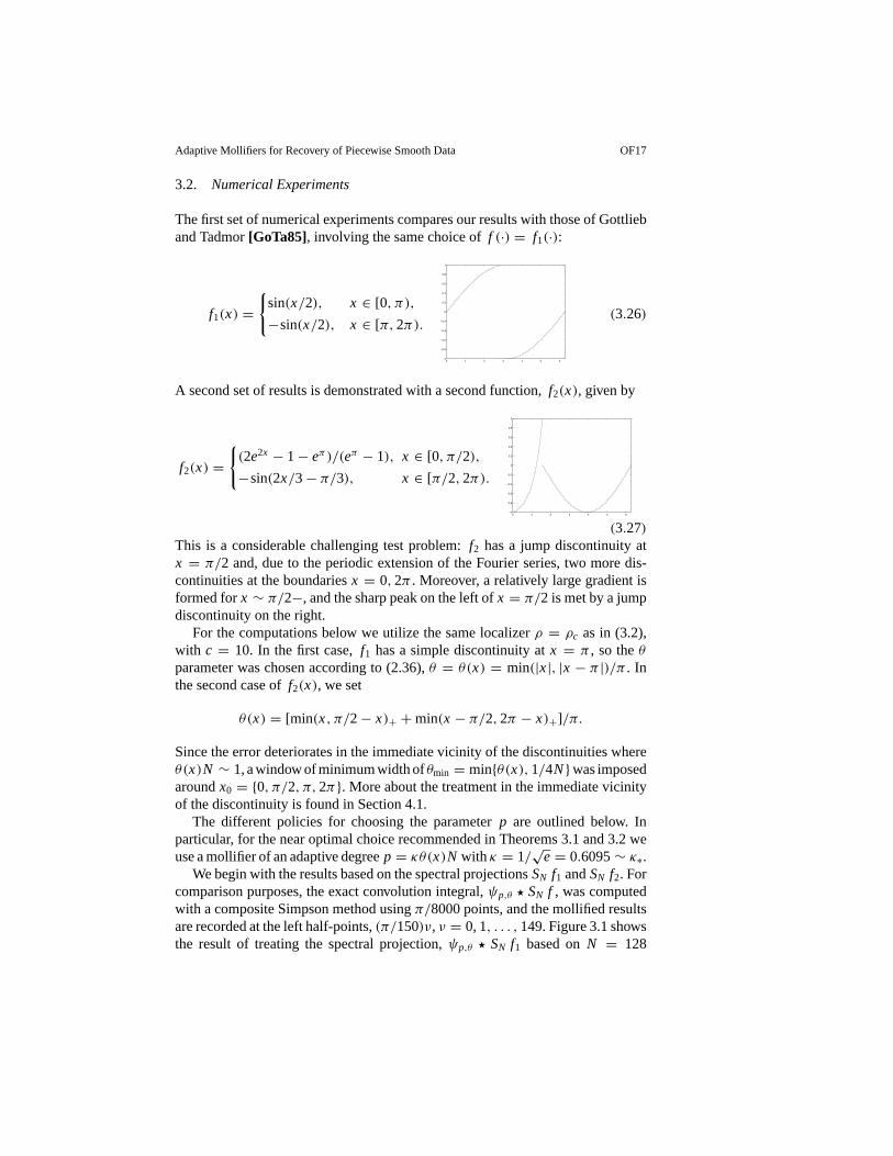
The first set of numerical experiments compares our results with those of Gottlieband Tadmor[GoTa85], involving the same choice off (·) = f1(·):
f1(x) ={
sin(x/2), x ∈ [0, π),
−sin(x/2), x ∈ [π,2π).
0 1 2 3 4 5 6−1
−0.8
−0.6
−0.4
−0.2
0
0.2
0.4
0.6
0.8
1
(3.26)
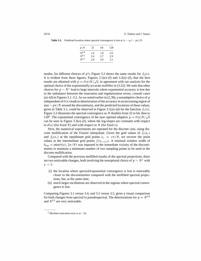
A second set of results is demonstrated with a second function,f2(x), given by
f2(x) ={(2e2x − 1− eπ )/(eπ − 1), x ∈ [0, π/2),
−sin(2x/3− π/3), x ∈ [π/2,2π).
0 1 2 3 4 5 6−1
−0.8
−0.6
−0.4
−0.2
0
0.2
0.4
0.6
0.8
1
(3.27)This is a considerable challenging test problem:f2 has a jump discontinuity atx = π/2 and, due to the periodic extension of the Fourier series, two more dis-continuities at the boundariesx = 0,2π . Moreover, a relatively large gradient isformed forx ∼ π/2−, and the sharp peak on the left ofx = π/2 is met by a jumpdiscontinuity on the right.
For the computations below we utilize the same localizerρ = ρc as in (3.2),with c = 10. In the first case,f1 has a simple discontinuity atx = π , so theθparameter was chosen according to (2.36),θ = θ(x) = min(|x|, |x − π |)/π . Inthe second case off2(x), we set
θ(x) = [min(x, π/2− x)+ +min(x − π/2,2π − x)+]/π.
Since the error deteriorates in the immediate vicinity of the discontinuities whereθ(x)N ∼ 1, a window of minimum width ofθmin = min{θ(x),1/4N}was imposedaroundx0 = {0, π/2, π,2π}. More about the treatment in the immediate vicinityof the discontinuity is found in Section 4.1.
The different policies for choosing the parameterp are outlined below. Inparticular, for the near optimal choice recommended in Theorems 3.1 and 3.2 weuse a mollifier of an adaptive degreep = κθ(x)N with κ = 1/
√e= 0.6095∼ κ∗.
We begin with the results based on the spectral projectionsSN f1 andSN f2. Forcomparison purposes, the exact convolution integral,ψp,θ ? SN f , was computedwith a composite Simpson method usingπ/8000 points, and the mollified resultsare recorded at the left half-points,(π/150)ν, ν = 0, 1, . . . ,149. Figure 3.1 showsthe result of treating the spectral projection,ψp,θ ? SN f1 based onN = 128
OF18 E. Tadmor and J. Tanner
Table 3.1. Predicted location where spectral convergence is lost at|x − x0| ∼ pπ/N.
p\N 32 64 128
N0.8 1.6 1.8 2.0N0.5 2.6 2.7 2.9N0.2 2.9 3.0 3.1
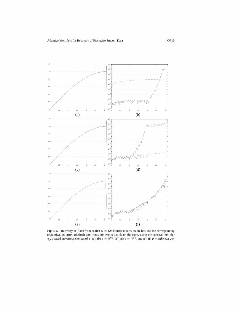
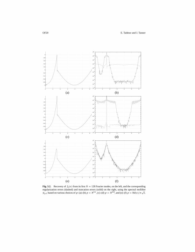
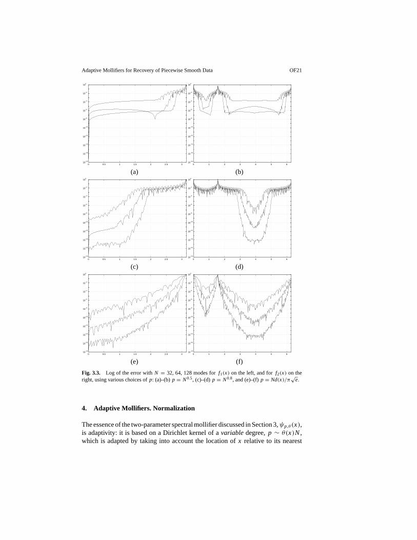
modes, for different choices ofp’s. Figure 3.2 shows the same results forf2(x).It is evident from these figures, Figures 3.1(e)–(f) and 3.2(e)–(f), that the bestresults are obtained withp = θ(x)N/√e, in agreement with our analysis for theoptimal choice of the exponentially accurate mollifier in (3.22). We note that otherchoices forp ∼ Nγ lead to large intervals where exponential accuracy is lost dueto the imbalance between the truncation and regularization errors, consult cases(a)–(d) in Figures 3.1–3.2. As we noted earlier in (2.38), a nonadaptive choice ofpindependent ofθ(x) leads to deterioration of the accuracy in an increasing region ofsize∼ pπ/N around the discontinuity, and the predicted locations of these values,given in Table 3.1, could be observed in Figure 3.1(a)–(d) for the functionf1(x).Figure 3.3 illustrates the spectral convergence asN doubles from 32 to 64, then to1286. The exponential convergence of the near optimal adaptivep = θ(x)N/√ecan be seen in Figure 3.3(e)–(f), where the log-slopes are constants with respectto d(x) (for fixed N) and with respect toN (for fixed x).
Next, the numerical experiments are repeated for the discrete case, using dis-crete mollification of the Fourier interpolant. Given the grid values off1(xν)and f2(xν) at the equidistant grid pointsxν = νπ/N, we recover the pointvalues at the intermediate grid pointsf (xν+1/2). A minimal window width ofθmin = min(θ(x),2π/N) was imposed in the immediate vicinity of the disconti-nuities to maintain a minimum number of two sampling points to be used in thediscrete mollification.
Compared with the previous mollified results of the spectral projections, thereare two noticeable changes, both involving the nonoptimal choice ofp ∼ Nγ withγ < 1:
(i) the location where spectral/exponential convergence is lost is noticeablycloser to the discontinuities compared with the mollified spectral projec-tions, but, at the same time,
(ii) much larger oscillations are observed in the regions where spectral conver-gence is lost.
Comparing Figures 3.1 versus 3.4, and 3.2 versus 3.5, gives a visual comparisonfor both changes from spectral to pseudospectral. The deteriorations forp = N0.8
andN0.5 are very noticeable.
6 Machine truncation error is at−16.
Adaptive Mollifiers for Recovery of Piecewise Smooth Data OF19
0 0.5 1 1.5 2 2.5 30
0.2
0.4
0.6
0.8
1
1.2
0 0.5 1 1.5 2 2.5 310
−18
10−16
10−14
10−12
10−10
10−8
10−6
10−4
10−2
100
(a) (b)
0 0.5 1 1.5 2 2.5 30
0.2
0.4
0.6
0.8
1
1.2
0 0.5 1 1.5 2 2.5 310
−18
10−16
10−14
10−12
10−10
10−8
10−6
10−4
10−2
100
(c) (d)
0 0.5 1 1.5 2 2.5 30
0.2
0.4
0.6
0.8
1
1.2
0 0.5 1 1.5 2 2.5 310
−18
10−16
10−14
10−12
10−10
10−8
10−6
10−4
10−2
100
(e) (f)
Fig. 3.1. Recovery off1(x) from its firstN = 128 Fourier modes, on the left, and the correspondingregularization errors (dashed) and truncation errors (solid) on the right, using the spectral mollifierψp,θ based on various choices ofp: (a)–(b)p = N0.5, (c)–(d)p = N0.8, and (e)–(f)p = Nd(x)/π
√e.
OF20 E. Tadmor and J. Tanner
0 1 2 3 4 5 6
−1
−0.8
−0.6
−0.4
−0.2
0
0.2
0.4
0.6
0.8
1
0 1 2 3 4 5 610
−18
10−16
10−14
10−12
10−10
10−8
10−6
10−4
10−2
100
(a) (b)
0 1 2 3 4 5 6
−1
−0.8
−0.6
−0.4
−0.2
0
0.2
0.4
0.6
0.8
1
0 1 2 3 4 5 610
−18
10−16
10−14
10−12
10−10
10−8
10−6
10−4
10−2
100
(c) (d)
0 1 2 3 4 5 6
−1
−0.8
−0.6
−0.4
−0.2
0
0.2
0.4
0.6
0.8
1
0 1 2 3 4 5 610
−18
10−16
10−14
10−12
10−10
10−8
10−6
10−4
10−2
100
(e) (f)
Fig. 3.2. Recovery off2(x) from its firstN = 128 Fourier modes, on the left, and the correspondingregularization errors (dashed) and truncation errors (solid) on the right, using the spectral mollifierψp,θ based on various choices ofp: (a)–(b)p = N0.5, (c)–(d)p = N0.8, and (e)–(f)p = Nd(x)/π
√e.
Adaptive Mollifiers for Recovery of Piecewise Smooth Data OF21
0 0.5 1 1.5 2 2.5 310
−18
10−16
10−14
10−12
10−10
10−8
10−6
10−4
10−2
100
0 1 2 3 4 5 610
−18
10−16
10−14
10−12
10−10
10−8
10−6
10−4
10−2
100
(a) (b)
0 0.5 1 1.5 2 2.5 310
−18
10−16
10−14
10−12
10−10
10−8
10−6
10−4
10−2
100
0 1 2 3 4 5 610
−18
10−16
10−14
10−12
10−10
10−8
10−6
10−4
10−2
100
(c) (d)
0 0.5 1 1.5 2 2.5 310
−18
10−16
10−14
10−12
10−10
10−8
10−6
10−4
10−2
100
0 1 2 3 4 5 610
−18
10−16
10−14
10−12
10−10
10−8
10−6
10−4
10−2
100
(e) (f)
Fig. 3.3. Log of the error withN = 32, 64, 128 modes forf1(x) on the left, and forf2(x) on theright, using various choices ofp: (a)–(b) p = N0.5, (c)–(d) p = N0.8, and (e)–(f)p = Nd(x)/π
√e.
4. Adaptive Mollifiers. Normalization
The essence of the two-parameter spectral mollifier discussed in Section 3,ψp,θ (x),is adaptivity: it is based on a Dirichlet kernel of avariabledegree,p ∼ θ(x)N,which is adapted by taking into account the location ofx relative to its nearest
OF22 E. Tadmor and J. Tanner
0 0.5 1 1.5 2 2.5 30
0.2
0.4
0.6
0.8
1
1.2
0 0.5 1 1.5 2 2.5 310
−18
10−16
10−14
10−12
10−10
10−8
10−6
10−4
10−2
100
(a) (b)
0 0.5 1 1.5 2 2.5 30
0.2
0.4
0.6
0.8
1
1.2
0 0.5 1 1.5 2 2.5 310
−18
10−16
10−14
10−12
10−10
10−8
10−6
10−4
10−2
100
(c) (d)
0 0.5 1 1.5 2 2.5 30
0.2
0.4
0.6
0.8
1
1.2
0 0.5 1 1.5 2 2.5 310
−18
10−16
10−14
10−12
10−10
10−8
10−6
10−4
10−2
100
(e) (f)
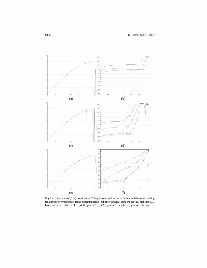
Fig. 3.4. Recovery off1(x) from itsN = 128 equidistant grid values on the left, and the correspondingregularization errors (dashed) and truncation errors (solid) on the right, using the spectral mollifierψp,θ
based on various choices ofp: (a)–(b) p = N0.5, (c)–(d) p = N0.8, and (e)–(f)p = Nd(x)/π√
e.
Adaptive Mollifiers for Recovery of Piecewise Smooth Data OF23
0 1 2 3 4 5 6
−1
−0.8
−0.6
−0.4
−0.2
0
0.2
0.4
0.6
0.8
1
0 1 2 3 4 5 610
−18
10−16
10−14
10−12
10−10
10−8
10−6
10−4
10−2
100
(a) (b)
0 1 2 3 4 5 6
−1
−0.8
−0.6
−0.4
−0.2
0
0.2
0.4
0.6
0.8
1
0 1 2 3 4 5 610
−18
10−16
10−14
10−12
10−10
10−8
10−6
10−4
10−2
100
(c) (d)
0 1 2 3 4 5 6
−1
−0.8
−0.6
−0.4
−0.2
0
0.2
0.4
0.6
0.8
1
0 1 2 3 4 5 610
−18
10−16
10−14
10−12
10−10
10−8
10−6
10−4
10−2
100
(e) (f)
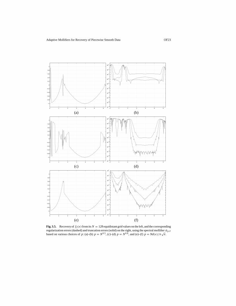
Fig. 3.5. Recovery off2(x) from itsN = 128 equidistant grid values on the left, and the correspondingregularization errors (dashed) and truncation errors (solid) on the right, using the spectral mollifierψp,θ
based on various choices ofp: (a)–(b) p = N0.5, (c)–(d) p = N0.8, and (e)–(f)p = Nd(x)/π√
e.
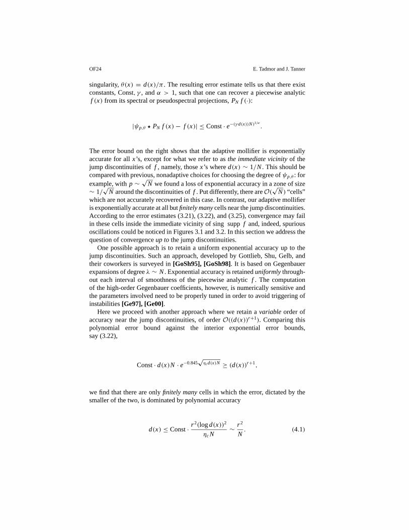
OF24 E. Tadmor and J. Tanner
singularity,θ(x) = d(x)/π . The resulting error estimate tells us that there existconstants, Const, γ , andα > 1, such that one can recover a piecewise analyticf (x) from its spectral or pseudospectral projections,PN f (·):
|ψp,θ ? PN f (x)− f (x)| ≤ Const· e−(γd(x))N)1/α .
The error bound on the right shows that the adaptive mollifier is exponentiallyaccurate for allx’s, except for what we refer to asthe immediate vicinityof thejump discontinuities off , namely, thosex’s whered(x) ∼ 1/N. This should becompared with previous, nonadaptive choices for choosing the degree ofψp,θ : forexample, withp ∼ √N we found a loss of exponential accuracy in a zone of size∼ 1/√
N around the discontinuities off . Put differently, there areO(√
N) “cells”which are not accurately recovered in this case. In contrast, our adaptive mollifieris exponentially accurate at all butfinitely manycells near the jump discontinuities.According to the error estimates (3.21), (3.22), and (3.25), convergence may failin these cells inside the immediate vicinity of sing suppf and, indeed, spuriousoscillations could be noticed in Figures 3.1 and 3.2. In this section we address thequestion of convergenceup tothe jump discontinuities.
One possible approach is to retain a uniform exponential accuracy up to thejump discontinuities. Such an approach, developed by Gottlieb, Shu, Gelb, andtheir coworkers is surveyed in[GoSh95], [GoSh98]. It is based on Gegenbauerexpansions of degreeλ ∼ N. Exponential accuracy is retaineduniformlythrough-out each interval of smoothness of the piecewise analyticf . The computationof the high-order Gegenbauer coefficients, however, is numerically sensitive andthe parameters involved need to be properly tuned in order to avoid triggering ofinstabilities[Ge97], [Ge00].
Here we proceed with another approach where we retain avariable order ofaccuracy near the jump discontinuities, of orderO((d(x))r+1). Comparing thispolynomial error bound against the interior exponential error bounds,say (3.22),
Const· d(x)N · e−0.845√ηcd(x)N ≥ (d(x))r+1,
we find that there are onlyfinitely manycells in which the error, dictated by thesmaller of the two, is dominated by polynomial accuracy
d(x) ≤ Const· r2(logd(x))2
ηcN∼ r 2
N. (4.1)
Adaptive Mollifiers for Recovery of Piecewise Smooth Data OF25
In this approach, the variable order of accuracy suggested by (4.1),r ∼ √d(x)N,is increasing together with the increasing distance away from the jumps or, moreprecisely, together with the number of cells away from the discontinuities, whichis consistent with theadaptivenature of our exponentially accurate mollifieraway from the immediate vicinity of these jumps. The current approach of avariable order of accuracy, which adapted to the distance from the jump dis-continuities, is reminiscent of the Essentially Non Oscillatory (ENO) piecewisepolynomial reconstruction employed in the context of nonlinear conservationlaws[HEOC85], [Sh97].
How do we enforce that our adaptive mollifiers are polynomially accurate inthe immediate vicinity of jump discontinuities? As we argued earlier in (2.11),the adaptive mollifierψp,θ admits spectrally small moments of orderp−s ∼(d(x)N)−s. More precisely, using (3.7), we find, forρ ∈ Gα:
∫ πθ
−πθysψp,θ (y)dy =
∫ π
−π(yθ)sρ(y)Dp(y)dy= Dp ? ((yθ)
sρ)(y)|y=0
= δs0+ Const· θs · e−α(ηp)1/α , p ∼ d(x)N.
Consequently,ψp,θ possesses exponentially small moments at allx’s except inthe immediate vicinity of the jumps wherep ∼ d(x)N ∼ 1, the sameO(1/N)neighborhoods where the previous exponential error bounds fail. This is illustratedin the numerical experiments exhibited in Section 3.2 which show the blurring insymmetric intervals with a width∼ 1/N around each discontinuity. To removethis blurring, we will impose a novelnormalizationso that finitely many momentsof (the projection of)ψp,θ preciselyvanish. As we shall see below, this will regaina polynomial convergence rate of the corresponding finite orderr . We have seenthat the general adaptivity (4.1) requiresr ∼ √d(x)N; in practice, enforcing afixed number of vanishing moments,r ∼ 2,3, will suffice.
4.1. Spectral Normalization. Adaptive Mollifiers in the Vicinity of Jumps
Rather thanψp,θ possessing a fixed number of vanishing moments, as in standardmollification (2.7), we require that its spectral projection,SNψp,θ , possess a unitmass and, sayr vanishing moments,∫ π
−πys(SNψp,θ )(y)dy= δs0, s= 0,1, . . . , r. (4.2)
It then follows that adaptive mollification of the Fourier projection,ψp,θ ? SN f ,recovers the point values off with the desired polynomial orderO(d(x))r .Indeed, noting that for eachx, the function f (x − y) remains smooth in theneighborhood|y| ≤ πθ = d(x) we find, utilizing the symmetry of the spectral
OF26 E. Tadmor and J. Tanner
projection,∫(SN f )g = ∫ f (SNg):
ψp,θ ? SN f (x)− f (x) =∫ πθ
−πθ[ f (x − y)− f (x)](SNψp,θ )(y)dy
=r∑
s=1
(−1)s
s!f (s)(x)
∫ π
−πys(SNψp,θ )(y)dy
+ (−1)r+1
(r + 1)!f (r+1)(·)
∫ π
−πyr+1(SNψp,θ )(y)dy
∼∫ π
−π(SN yr+1)ψp,θ (y)dy≤ Const·
(d(x)+ 1
N
)r+1
.
The last step follows from an upper bound for the spectral projection of monomialsoutlined at the end of this subsection.
To enforce the vanishing moments condition (4.2) on the adaptive mollifier,ψp,θ (·) = (ρ(·)Dp(·/θ))/θ , we take advantage of the freedom we have in choosingthe localizerρ(·). We begin by normalizing
ψ̃p,θ (y) = ψp,θ (y)∫ π−π ψp,θ (z)dz
so that̃ψp,θ has a unit mass, and hence (4.2) holds forr = 0, for∫
SN(ψp,θ )(y)dy= ∫ ψp,θ (y)dy = 1. We note that the resulting mollifier takes the same form asbefore, namely,
ψ̃p,θ (y) := 1
θ(ρ̃cDp)
( y
θ
), (4.3)
where the only difference is associated with the modified localizer
ρ̃c(y) = q0 · ρc(y), q0 = 1∫ π−π ψp,θ (z)dz
. (4.4)
Observe that, in fact, 1/q0 =∫ψp,θ (z)dz≡ ∫ ψp(z)dz= (Dp ? ρc)(0) and that,
with our choice ofp = κ · θ(x)N, we have, in view of (3.7),
ρ̃c(0) = q0 = 1
(Dp ? ρc)(0)= 1+O(ε),
ε ∼ d(x)N · e−2√ηc p, p = κ · θ(x)N,
which is admissible within the same exponentially small error bound we had before,consult (3.11). In other words, we are able to modify the localizerρc(·)→ ρ̃c(·)to satisfy the first-order normalization, (4.2), withr = 0, while the correspondingmollifier, (ρx Dp)θ → (ρ̃cDp)θ , retains the same overall exponential accuracy.Moreover, using evenρ’s implies thatψ(·) is an even function and hence its odd
Adaptive Mollifiers for Recovery of Piecewise Smooth Data OF27
moments vanish. Consequently, (4.2) holds withr = 1, and we end up with thefollowing quadratic error bound in the vicinity ofx (compared with (3.22)):
|ψ̃p,θ (x) ? SN f (x)− f (x)| ≤ Const·(
d(x)+ 1
N
)2
· e−0.845√ηcd(x)N .
In a similar manner, we can enforce higher vanishing moments by propernormal-izationof the localizerρ(·). There is clearly more than one way to proceed—hereis one possibility. In order to satisfy (4.2) withr = 2 we use a prefactor of the formρ̃c(x) ∼ (1+ q2x2)ρc(x). Imposing a unit mass and a vanishing second momentwe may take
ψ̃p,θ (y) = 1
θ(ρ̃cDp)
( y
θ
), ρ̃c(y) ∼ (1+ q2y2)ρc(y),
with the normalized localizer,̃ρc(y), given by
ρ̃c(y) = 1+ q2y2∫ π−π (1+ q2(z/θ)2)ψp,θ (z)dz
ρc(y),
q2 =− ∫ π−π (SNz2)ψp,θ (z)dz∫ π−π (SNz2)(z/θ)2ψp,θ (z)dz
. (4.5)
As before, the resulting mollifier̃ψp,θ is admissible in the sense of satisfyingthe normalization (3.11) within the exponentially small error term. Indeed, since∫
y2ψp,θ (y)dy= (Dp ? (y2ρc(y)))(0) = O(ε), we find
ρ̃c(0) = 1∫ π−π (1+ q2(y/θ)2)ψp,θ (y)dy
= 1
1+ q2 · ε/θ2= 1+ Const· (d(x)N)3 · e−2
√ηc p, p = κ · θ(x)N.
A straightforward computation shows that the unit massψ̃p,θ has a second van-ishing moment∫ π
−πy2(SNψ̃p,θ )(y)dy =
∫ π
−π(SN y2)
(a0+ a2
( y
θ
)2)ψp,θ (y)dy
=∫ π
−π(SN y2)ψp,θ (y)dy
+ q2
∫ π
−π(SN y2)
( y
θ
)2ψp,θ (y)dy= 0. (4.6)
Sinceρ̃c(·) is even, so is the normalized mollifier̃ψ(·), and hence its third momentvanishes yielding a fourth-order convergence rate in the immediate vicinity of thejump discontinuities
|(ψ̃p,θ (x) ? SN f )(x)− f (x)| ≤ Const·(
d(x)+ 1
N
)4
· e−0.845√ηcd(x)N .
OF28 E. Tadmor and J. Tanner
We close this section with the promised
Lemma 4.1[Tao]. The following pointwise estimate holds
|SN(yr )| .
(|y| + 1
N
)r
.
To prove this, we use a dyadic decomposition (similar to the Littlewood–Paleyconstruction) to split
yr =∑k≤0
2krψ(y/2k)
whereψ is a bump function adapted to the set{π/4< |y| < π}.For 2k . 1/N, the usual upperbounds of the Dirichlet kernel tell us that
|SN(ψ(·/2k))(y)| . 2k N/(1+ N|y|).Now suppose 2k & 1/N. In this case we can use the rapid decay of the Fouriertransform ofψ(·/2k), for frequenciesÀ N, to obtain the estimate
‖(1− SN)(ψ(·/2k))‖∞ . (2k N)−100.
In particular, since suppψ ∼ 1, we have|SN(ψ(·/2k))(x)| . 1 when|y| ∼ 2k, and|SN(ψ(·/2k))(y)| . (2k N)−100 otherwise. The desired bound follows by addingtogether all these estimates overk.
4.2. Pseudospectral Normalization. Adaptive Mollifiers in the Vicinity of Jumps
We now turn to the pseudospectral case which will only require evaluations ofdiscrete sums and, consequently, can be implemented with little increase in com-putation time.
Let f ∗ g(x) := ∑ν f (x − yν)g(yν)h denote the (noncommutative) discreteconvolution based on 2N equidistant grid points,yν = νh, h = π/N. Noting thatfor eachx, the functionf (y) remains smooth in the neighborhood|x− y| ≤ πθ =d(x), we find
|ψp,θ ∗ IN f (x)− f (x)| =∣∣∣∣∣∑ν
ψp,θ (x − yν)[ f (yν)− f (x)]h
∣∣∣∣∣=∣∣∣∣∣ r∑
s=1
(−1)s
s!f (s)(x)
∑ν
(x − yν)sψp,θ (x − yν)h
+ (−1)r+1
(r + 1)!f (r+1)(·)
∑ν
(x − yν)r+1ψp,θ (x − yν)h
∣∣∣∣∣≤ Const· (d(x))r+1, Const∼
‖ f ‖Cr+1loc
(r + 1)!,
Adaptive Mollifiers for Recovery of Piecewise Smooth Data OF29
providedψp,θ has its firstr discretemoments vanish
2N−1∑ν=0
(x − yν)sψp,θ (x − yν)h = δs0, s= 0,1,2, . . . , r. (4.7)
Observe that, unlike the continuous case associated with spectral projections,the discrete constraint (4.7) is not translation invariant and hence it requiresx-dependent normalizations. The additional computational effort is minimal, how-ever, due to the discrete summations which are localized in the immediate vicinityof x. Indeed, as a first step, we note the validity of (4.7) forx’s which are awayfrom the immediate vicinity of the jumps off . To this end, we apply the mainexponential error estimate (3.25) forf (·) = (x − ·)s (for arbitrary fixedx), toobtain
2N−1∑ν=0
(x − yν)sψp,θ (x − yν)h = (x − y)s|y=x +O(ε) = δs0+O(ε),
ε ∼ (d(x)N)2 · e−√
Const·d(x)·N . (4.8)
Thus, (4.7) holds modulo exponentially small error for thosex’s which are awayfrom the jumps off , whered(x) À 1/N. The issue now is to enforce discretevanishing moments on the adaptive mollifierψp(x) = ρ(x)Dp(x) in the vicinityof these jumps and, to this end, we take advantage of the freedom we have inchoosing the localizerρ(·). We begin by normalizing
ψ̃p,θ (y) = ψp,θ (y)∑2N−1ν=0 ψp,θ (x − yν)h
,
so thatψ̃p,θ (x− ·) has a (discrete) unit mass, i.e., (4.7) holds withr = 0. We notethat the resulting mollifier takes the same form as before, namely,
ψ̃p,θ (y) := 1
θ(ρ̃cDp)
( y
θ
), (4.9)
and that the only difference is associated with the modified localizer
ρ̃c(y) = q0 · ρc(y), q0 = 1∑2N−1ν=0 ψp,θ (x − yν)h
. (4.10)
By (4.8), thex-dependent normalization factor,q0 = q0(x) is, in fact, an approxi-mate identity
1/q0 =2N−1∑ν=0
ψp,θ (x − yν)h = 1+O(ε), ε ∼ (d(x)N)2 · e−√
Const·d(x)·N,
which shows that the normalized localizer is admissible,|ρ̃(0) − 1| = |q0 −1| ≤ O(ε), within the same exponentially small error bound we had before,
OF30 E. Tadmor and J. Tanner
consult (3.11) with our choice ofp ∼ d(x) · N. In other words, we are ableto modify the localizerρc(·) → ρ̃c(·) to satisfy the first-order normalization,(4.7), with r = 0 required near jump discontinuities, while the correspondingmollifier, (ρx Dp)θ → (ρ̃cDp)θ , retains the same overall exponential accuracyrequired outside the immediate vicinity of these jumps.
Next, we turn to enforcing that the first discrete moment vanishes,∑
ν(x −yν)ψ̃p,θ (x − yν)h = 0 and, to this end, we seek a modified mollifier of the form
ψ̃p,θ (y) = q(y/θ)∑ν q
(x − yνθ
)ψp,θ (x − yν)h
ψp,θ (y), q(y) := 1+ q1y,
with q1 chosen so that the second constraint, (4.7) withr = 1, is satisfied7
q1 = −∑
ν(x − yν)ψp,θ (x − yν)h∑ν
(x − yν)2
θψp,θ (x − yν)h
. (4.11)
Consequently, (4.7) holds withr = 1, and we end up with a quadratic error boundcorresponding to (3.22):
|ψ̃p,θ ∗ IN f (x)− f (x)| ≤ Const· (d(x))2 · e−√
Const·d(x)N .
Moreover, (4.8) implies thatq1 = O(ε) and hence the new normalized localizer isadmissible,ρ̃c(0) = 1+O(ε). In a similar manner we can treat higher momentsusingnormalizedlocalizers,ρ̃c(y) ∼ q(y)ρc(y), of the form
ψ̃p,θ (y) = 1
θ(ρ̃cDp)
( y
θ
),
ρ̃c(y) := 1+ q1y+ · · · + qr yr∑ν q
(x − yνθ
)ψp,θ (x − yν)h
ρc(y). (4.12)
Ther free coefficients ofq(y) = 1+q1y+ · · ·+qr yr are chosen so as to enforce(4.7) so that the firstr discrete moments of̃ψ vanish. This leads to a simpler × r Vandermonde system (outlined at the end of this section) involving thergrid values,{ f (yν)}, in the vicinity of x, |yν − x| ≤ θ(x)π . With our choice ofa symmetric support of sizeθ(x) = d(x)/π , there are preciselyr = 2θπ/h =2Nd(x)/π such grid points in the immediate vicinity ofx, which enable us torecover the intermediate grid values,f (x), with an adaptiveorder, (d(x))r+1,
7 We note, in passing, that̃ρc(·) being even implies that̃ψp,θ (·) is an even function and hence itsodd moments vanish. It follows that the first discrete moment,
∑ν(x− yν)ψp,θ (x− yν)h, vanishes at
the grid pointsx = yµ, and thereforeq1 = 0 there. But otherwise, unlike the similar situation with thespectral normalization,q1 6= 0. The discrete summation inq1, however, involves only finitely manyneighboring values in theθ -vicinity of x.
Adaptive Mollifiers for Recovery of Piecewise Smooth Data OF31
r ∼ Nd(x). As before, this normalization does not affect the exponential accuracyaway from the jump discontinuities, noting thatρ̃(0)c = 1/q0 = 1 + O(ε) inagreement with (3.11). We summarize by stating
Theorem 4.1. Given the equidistant gridvalues, { f (xν)}0≤ν≤2N−1 of a piecewiseanalytic f(·), we want to recover the intermediate values f(x). To this end, weuse the two-parameter family of pseudospectral mollifiers
ψ̃p,θ (y) := 1
θρ̃c
( y
θ
)Dp
( y
θ
), p = 0.5596· θN, c > 0,
whereθ = θ(x) := d(x)/π is the (scaled) distance between x and its nearestjump discontinuity. We setρ̃c(y) := q(y)e(cy2/(y2−π2))1[−π,π ] as the normalizingfactor, with
q(y) = 1+ q1y+ · · · + qr yr∑ν q
(x − yνθ
)ψp,θ (x − yν)h
so that the first r discrete moments ofψ̃p,θ (y) vanish, i.e., (4.7)holds with r ∼Nd(x).
Then there exist constants, Constc andηc, depending solely on the analytic be-havior of f(·) in the neighborhood of x, such that we can recover the intermediatevalues of f(x) with the following exponential accuracy∣∣∣∣∣ πN
2N−1∑ν=0
ψp,θ (x − yν) f (yν)− f (x)
∣∣∣∣∣≤ Constc · (d(x))r+1
(1
e
)0.845√ηcd(x)N
, r ∼ Nd(x). (4.13)
The error bound (4.13) confirms our statement in the introduction of Section 4,namely, theadaptivityof the spectral mollifier, in the sense of recovering the gridvalues in the vicinity of the jumps with an increasing order,Nd(x), is proportionalto their distance from sing suppf . We have seen that the general adaptivity (4.1)requiresr ∼ √d(x)N so that, in practice, enforcing a fixed number of vanishingmoments,r ∼ 2,3, will suffice as a transition to the exponentially error decay inthe interior region of smoothness. We highlight the fact that the modified mollifierψ̃p,θ , normalized by having finitely many (∼ 2,3) vanishing moments, can be con-structed with little increase in computation time and, as we will see in Section 4.3below, it yields greatly improved results near the discontinuities.
We close this section with a brief outline of the construction of ther -order accu-rate normalization factorq(·). To recoverf (x), we seek anr -degree polynomial,q(y) := 1+ q1y + · · · + qr yr , so that (4.7) holds. We emphasize that theqr ’sdepend on the specific pointx in the following manner. Settingzν := x− yν , then
OF32 E. Tadmor and J. Tanner
satisfying (4.7) for thehighermoments of̃ψp,θ , requires∑ν
zsνψ̃p,θ (zν)h = 0, s= 1,2, . . . , r,
and withψ̃p,θ (·) ∼ q(·/θ)ψp,θ (·) we end up with∑ν
zsν
[q(zνθ
)− 1
]ψp,θ (zν)h = −
∑ν
zsνψp,θ (zν), s= 1,2, . . . , r.
Expressed in terms of the discrete moments ofψ :
aα(zν) :=∑ν
(zνθ
)1+αψp,θ (zν), α = 1,2, . . . ,2r,
this amounts to ther × r Vandermonde-like system for{q1, . . . ,qr }:a1(zν) a2(zν) · · · ar (zν)
· · · · · ·· · · · · ·· · · · · ·
ar+1(zν) ar+2(zν) · · · a2r (zν)
q1
···
qr
=−
∑ν zνψp,θ (zν)
···∑
ν zrνψp,θ (zν)
. (4.14)
Finally, we scaleq(·) so that(4.7) holds withs= 0, which led us to the normalizedlocalizer in (4.12).
4.3. Numerical Experiments
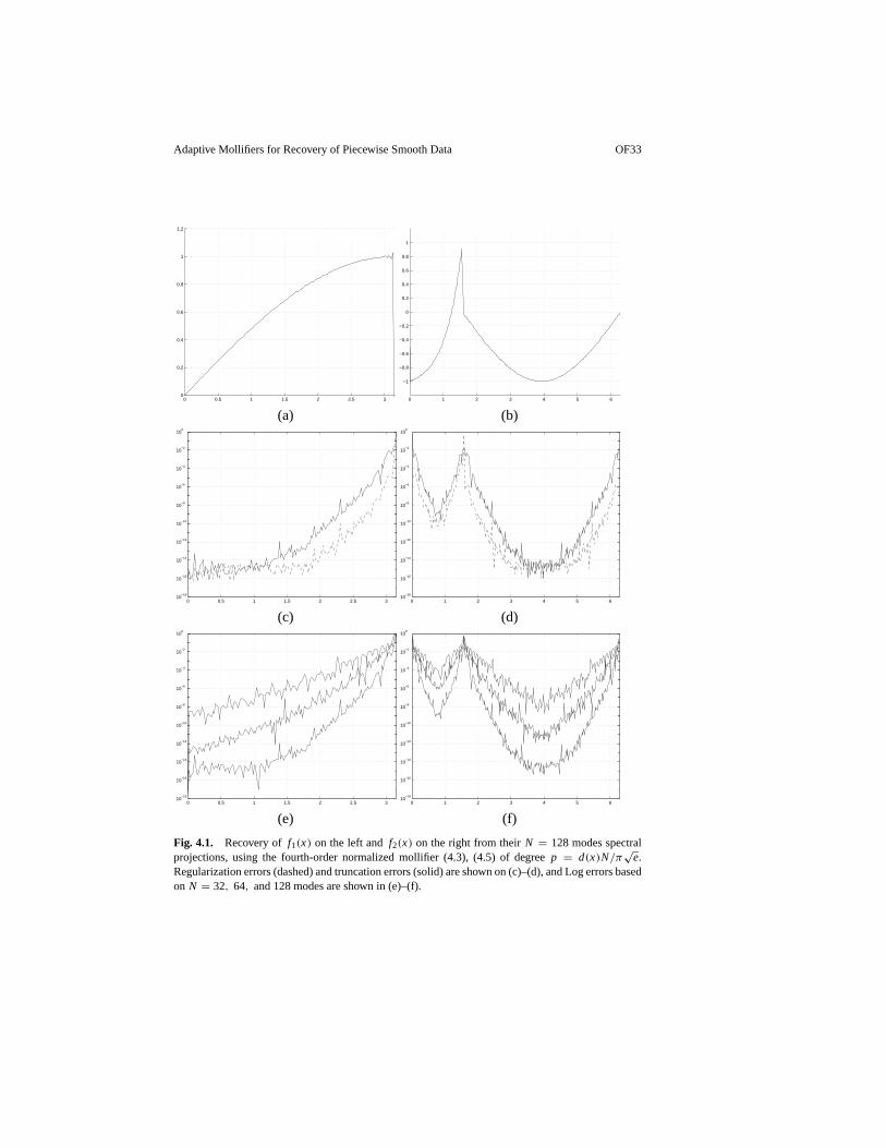
Figure 3.1(d) shows the blurring oscillations near the edges when using the non-normalized adaptive mollifier. To reduce this blurring we will use the normalizedψ̃p,θ for x’s in the vicinity of the jumps whered(x) ≤ 6π/N. The convolutionis computed at the same locations as in Section 3.2, and a minimum windowwidth of θ(x) = min(d(x)/π,2π/N) was imposed. The trapezoidal rule (withspacing ofπ/8000) was used for the numerical integration of(SN y2)ψp,θ (y) and(SN y2)y2ψp,θ (y), required for the computation ofq0 andq2 in Figure 4.1. Fig-ure 4.1(a)–(d) shows the clear improvement near the edges once we utilize thenormalizedψ̃p,θ , while retaining the exponential convergence away from theseedges is illustrated in Figure 4.1(e)–(f).
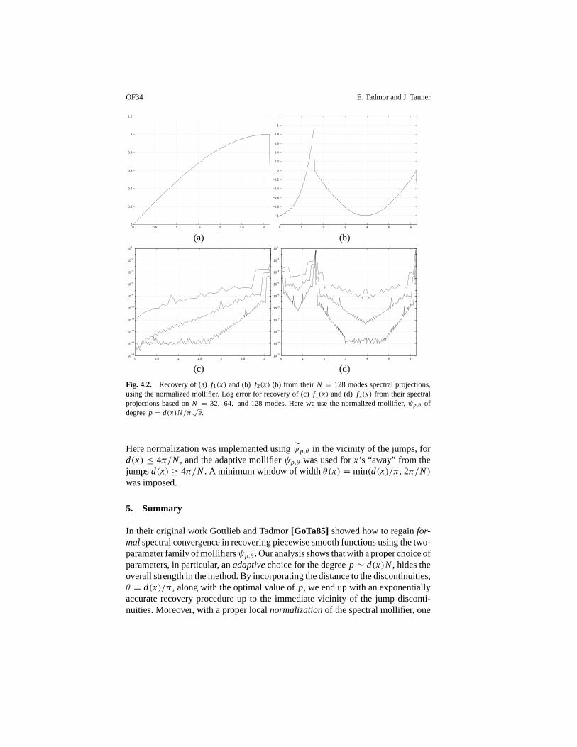
We conclude with the pseudospectral case. TheO(1) error remains in Fig-ure 3.4(d) for the non-normalized mollifier. The normalization of the discretemollifier in Section 4.2 shows that by using̃ψp,θ given in (4.12), with a fourth-degree normalization factorq(·), results in a minimum convergence rate ofd(x)4
in the vicinity of the jumps, and with exponentially increasing order as we moveaway from the jumps. This modification of̃ψp,θ leads to a considerable improve-ment in the resolution near the discontinuity, which can be seen in Figure 4.2.
Adaptive Mollifiers for Recovery of Piecewise Smooth Data OF33
0 0.5 1 1.5 2 2.5 30
0.2
0.4
0.6
0.8
1
1.2
0 1 2 3 4 5 6
−1
−0.8
−0.6
−0.4
−0.2
0
0.2
0.4
0.6
0.8
1
(a) (b)
0 0.5 1 1.5 2 2.5 310
−18
10−16
10−14
10−12
10−10
10−8
10−6
10−4
10−2
100
0 1 2 3 4 5 610
−18
10−16
10−14
10−12
10−10
10−8
10−6
10−4
10−2
100
(c) (d)
0 0.5 1 1.5 2 2.5 310
−18
10−16
10−14
10−12
10−10
10−8
10−6
10−4
10−2
100
0 1 2 3 4 5 610
−18
10−16
10−14
10−12
10−10
10−8
10−6
10−4
10−2
100
(e) (f)
Fig. 4.1. Recovery of f1(x) on the left andf2(x) on the right from theirN = 128 modes spectralprojections, using the fourth-order normalized mollifier (4.3), (4.5) of degreep = d(x)N/π
√e.
Regularization errors (dashed) and truncation errors (solid) are shown on (c)–(d), and Log errors basedon N = 32, 64, and 128 modes are shown in (e)–(f).
OF34 E. Tadmor and J. Tanner
0 0.5 1 1.5 2 2.5 30
0.2
0.4
0.6
0.8
1
1.2
0 1 2 3 4 5 6
−1
−0.8
−0.6
−0.4
−0.2
0
0.2
0.4
0.6
0.8
1
(a) (b)
0 0.5 1 1.5 2 2.5 310
−18
10−16
10−14
10−12
10−10
10−8
10−6
10−4
10−2
100
0 1 2 3 4 5 610
−18
10−16
10−14
10−12
10−10
10−8
10−6
10−4
10−2
100
(c) (d)
Fig. 4.2. Recovery of (a)f1(x) and (b) f2(x) (b) from their N = 128 modes spectral projections,using the normalized mollifier. Log error for recovery of (c)f1(x) and (d) f2(x) from their spectralprojections based onN = 32, 64, and 128 modes. Here we use the normalized mollifier,ψp,θ ofdegreep = d(x)N/π
√e.
Here normalization was implemented usingψ̃p,θ in the vicinity of the jumps, ford(x) ≤ 4π/N, and the adaptive mollifierψp,θ was used forx’s “away” from thejumpsd(x) ≥ 4π/N. A minimum window of widthθ(x) = min(d(x)/π,2π/N)was imposed.
5. Summary
In their original work Gottlieb and Tadmor[GoTa85] showed how to regainfor-malspectral convergence in recovering piecewise smooth functions using the two-parameter family of mollifiersψp,θ . Our analysis shows that with a proper choice ofparameters, in particular, anadaptivechoice for the degreep ∼ d(x)N, hides theoverall strength in the method. By incorporating the distance to the discontinuities,θ = d(x)/π , along with the optimal value ofp, we end up with an exponentiallyaccurate recovery procedure up to the immediate vicinity of the jump disconti-nuities. Moreover, with a proper localnormalizationof the spectral mollifier, one
Adaptive Mollifiers for Recovery of Piecewise Smooth Data OF35
can further reduce the error in the vicinity of these jumps. For the pseudospectralcase, the normalization adds little to the overall computation time. Overall, thisyields a high resolution yet very robust recovery procedure which enables one toeffectively manipulate pointwise values of piecewise smooth data.
Acknowledgment
Research was supported in part by ONR Grant No. N00014-91-J-1076 and NSFGrant No. DMS01-07428.
References
[BL93] R. K. Beatson and W. A. Light, Quasi-interpolation by thin-plate splines on the square,Constr. Approx. 9 (1993), 343–372.
[Ch] E. W. Cheney,Approximation Theory, Chelsea, New York, 1982.[Ge97] A. Gelb, The resolution of the Gibbs phenomenon for spherical harmonics,Math. Comp.
66 (1997), 699–717.[Ge00] A. Gelb, A hybrid approach to spectral reconstruction of piecewise smooth functions,J.
Sci. Comput. 15 (2000), 293–322.[GeTa99] A. Gelb and E. Tadmor, Detection of edges in spectral data,Appl. Comput. Harmonic Anal.
7 (1999), 101–135.[GeTa00a] A. Gelb and E. Tadmor, Enhanced spectral viscosity approximations for conservation laws,
Appl. Numer. Math. 33 (2000), 3–21.[GeTa00b] A. Gelb and E. Tadmor, Detection of edges in spectral data II. Nonlinear enhancement,
SIAM J. Numer. Anal. 38 (2000), 1389–1408.[GoSh95] D. Gottlieb and C.-W. Shu, On the Gibbs phenomenon IV: Recovering exponential accuracy
in a subinterval from a Gegenbauer partial sum of a piecewise analytic function,Math.Comp. 64 (1995), 1081–1095.
[GoSh98] D. Gottlieb and C.-W. Shu, On the Gibbs phenomenon and its resolution,SIAM Rev. 39(1998), 644–668.
[GoTa85] D. Gottlieb and E. Tadmor, Recovering pointwise values of discontinuous data withinspectral accuracy, in Progress and Supercomputing in Computational Fluid Dynamics,Proceedings of1984U.S.–Israel Workshop, Progress in Scientific Computing, Vol. 6 (E. M.Murman and S. S. Abarbanel, eds.), Birkhauser, Boston, 1985, pp. 357–375.
[HEOC85] A. Harten, B. Engquist, S. Osher, and S. R. Chakravarthy, Uniformly high order accurateessentially non-oscillatory schemes, III,J. Comput. Phys. 71 (1982), 231–303.
[Jo] F. John, Partial Differential Equations, 4th ed., Springer-Verlag, New York, 1982.[MMO78] A. Majda, J. McDonough, and S. Osher, The Fourier method for nonsmooth initial data,
Math. Comp. 30 (1978), 1041–1081.[Sh97] C.-W. Shu, Essentially nonoscillatory and weighted essentially nonoscillatory schemes
for hyperbolic conservation laws, inAdvanced Numerical Approximation of NonlinearHyperbolic Equations(A. Quarteroni, ed.). Lecture Notes in Mathematics #1697. Cetraro,Italy, Springer, New York, 1997.
[Ta94] E. Tadmor, Spectral methods for hyperbolic problems, from Lecture Notes Deliv-ered at Ecole Des Ondes, January 24–28, 1994. Available at http://www.math.ucla.edu/˜tadmor/pub/spectral-approximations/Tadmor.INRIA-94.pdf
[Tao] T. Tao, Private communication.