Foundations of Preference Queries
238
Foundations of Preference Queries Jan Chomicki University at Buffalo Jan Chomicki () Preference Queries 1 / 68
Transcript of Foundations of Preference Queries

Foundations of Preference Queries
Jan ChomickiUniversity at Buffalo
Jan Chomicki () Preference Queries 1 / 68

Plan of the course
1 Preference relations
2 Preference queries
3 Preference management
4 Advanced topics
Jan Chomicki () Preference Queries 2 / 68

Part I
Preference relations
Jan Chomicki () Preference Queries 3 / 68

Outline of Part I
1 Preference relationsPreferenceEquivalencePreference specificationCombining preferencesSkylines
Jan Chomicki () Preference Queries 4 / 68

Preference relations
Universe of objects
constants: uninterpreted, numbers,...
individuals (entities)
tuples
sets
Preference relation �binary relation between objects
x � y ≡ x is better than y ≡ x dominates y
an abstract, uniform way of talking about desirability, worth, cost,timeliness,..., and their combinations
preference relations used in queries
Jan Chomicki () Preference Queries 5 / 68

Buying a car
Salesman: What kind of car do you prefer?Customer: The newer the better, if it is the same make. And cheap, too.Salesman: Which is more important for you: the age or the price?Customer: The age, definitely.Salesman: Those are the best cars, according to your preferences, that wehave in stock.Customer: Wait...it better be a BMW.
Jan Chomicki () Preference Queries 6 / 68

Buying a car
Salesman: What kind of car do you prefer?
Customer: The newer the better, if it is the same make. And cheap, too.Salesman: Which is more important for you: the age or the price?Customer: The age, definitely.Salesman: Those are the best cars, according to your preferences, that wehave in stock.Customer: Wait...it better be a BMW.
Jan Chomicki () Preference Queries 6 / 68

Buying a car
Salesman: What kind of car do you prefer?Customer: The newer the better, if it is the same make. And cheap, too.
Salesman: Which is more important for you: the age or the price?Customer: The age, definitely.Salesman: Those are the best cars, according to your preferences, that wehave in stock.Customer: Wait...it better be a BMW.
Jan Chomicki () Preference Queries 6 / 68

Buying a car
Salesman: What kind of car do you prefer?Customer: The newer the better, if it is the same make. And cheap, too.Salesman: Which is more important for you: the age or the price?
Customer: The age, definitely.Salesman: Those are the best cars, according to your preferences, that wehave in stock.Customer: Wait...it better be a BMW.
Jan Chomicki () Preference Queries 6 / 68

Buying a car
Salesman: What kind of car do you prefer?Customer: The newer the better, if it is the same make. And cheap, too.Salesman: Which is more important for you: the age or the price?Customer: The age, definitely.
Salesman: Those are the best cars, according to your preferences, that wehave in stock.Customer: Wait...it better be a BMW.
Jan Chomicki () Preference Queries 6 / 68

Buying a car
Salesman: What kind of car do you prefer?Customer: The newer the better, if it is the same make. And cheap, too.Salesman: Which is more important for you: the age or the price?Customer: The age, definitely.Salesman: Those are the best cars, according to your preferences, that wehave in stock.
Customer: Wait...it better be a BMW.
Jan Chomicki () Preference Queries 6 / 68

Buying a car
Salesman: What kind of car do you prefer?Customer: The newer the better, if it is the same make. And cheap, too.Salesman: Which is more important for you: the age or the price?Customer: The age, definitely.Salesman: Those are the best cars, according to your preferences, that wehave in stock.Customer: Wait...it better be a BMW.
Jan Chomicki () Preference Queries 6 / 68

Applications of preferences and preference queries
1 decision making
2 e-commerce
3 digital libraries
4 personalization
Jan Chomicki () Preference Queries 7 / 68

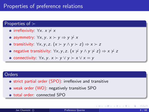
Properties of preference relations
Properties of �irreflexivity: ∀x . x 6� x
asymmetry: ∀x , y . x � y ⇒ y 6� x
transitivity: ∀x , y , z . (x � y ∧ y � z)⇒ x � z
negative transitivity: ∀x , y , z . (x 6� y ∧ y 6� z)⇒ x 6� z
connectivity: ∀x , y . x � y ∨ y � x ∨ x = y
Orders
strict partial order (SPO): irreflexive and transitive
weak order (WO): negatively transitive SPO
total order: connected SPO
Jan Chomicki () Preference Queries 8 / 68

Weak and total orders
Weak order
a b
c d e
f
Total order
a
d
f
Jan Chomicki () Preference Queries 9 / 68

Order properties of preference relations
Irreflexivity, asymmetry: uncontroversial.
Transitivity:
captures rationality of preference
not always guaranteed: voting paradoxes
helps with preference querying
Negative transitivity:
scoring functions represent weak orders
We assume that preference relations are SPOs.
Jan Chomicki () Preference Queries 10 / 68

When are two objects equivalent?
Relation ∼binary relation between objects
x ∼ y ≡ x ′′is equivalent to ′′ y
Several notions of equivalence
equality: x ∼eq y ≡ x = y
indifference: x ∼i y ≡ x � y ∧ y � x
restricted indifference:x ∼r y ≡ ∀z . (x ≺ z ⇔ y ≺ z) ∧ (z ≺ y ⇔ z ≺ x)
Properties of equivalence
equivalence relation: reflexive, symmetric, transitive
equality and restricted indifference (if � is an SPO) are equivalencerelations
indifference is reflexive and symmetric; transitive for WO
Jan Chomicki () Preference Queries 11 / 68

When are two objects equivalent?
Relation ∼binary relation between objects
x ∼ y ≡ x ′′is equivalent to ′′ y
Several notions of equivalence
equality: x ∼eq y ≡ x = y
indifference: x ∼i y ≡ x � y ∧ y � x
restricted indifference:x ∼r y ≡ ∀z . (x ≺ z ⇔ y ≺ z) ∧ (z ≺ y ⇔ z ≺ x)
Properties of equivalence
equivalence relation: reflexive, symmetric, transitive
equality and restricted indifference (if � is an SPO) are equivalencerelations
indifference is reflexive and symmetric; transitive for WOJan Chomicki () Preference Queries 11 / 68

Example
bmw
ford vw mazda
kia
This is a strict partialorder which is not aweak order.
Preference:
bmw � ford, bmw � vwbmw � mazda, bmw � kiamazda � kia
Indifference:
ford ∼i vw, vw ∼i ford,ford ∼i mazda, mazda ∼i
ford,vw ∼i mazda, mazda ∼i
vw,ford ∼i kia, kia ∼i ford,vw ∼i kia, kia ∼i vw
Restricted indifference:
ford ∼r vw, vw ∼r ford
Jan Chomicki () Preference Queries 12 / 68

Not every SPO is a WO
Canonical example
mazda � kia, mazda ∼i vw, kia ∼i vw
Violation of negative transitivity
mazda � vw, vw � kia, mazda � kia
Jan Chomicki () Preference Queries 13 / 68

Preference specification
Explicit preference relations
Finite sets of pairs: bmw � mazda, mazda � kia,...
Implicit preference relations
can be infinite but finitely representable
defined using logic formulas in some constraint theory:
(m1, y1, p1) �1 (m2, y2, p2) ≡ y1 > y2 ∨ (y1 = y2 ∧ p1 < p2)
for relation Car(Make,Year ,Price).
defined using preference constructors (Preference SQL)
defined using real-valued scoring functions: F (m, y , p) = α · y + β · p(m1, y1, p1) �2 (m2, y2, p2) ≡ F (m1, y1, p1) > F (m2, y2, p2)
Jan Chomicki () Preference Queries 14 / 68

Preference specification
Explicit preference relations
Finite sets of pairs: bmw � mazda, mazda � kia,...
Implicit preference relations
can be infinite but finitely representable
defined using logic formulas in some constraint theory:
(m1, y1, p1) �1 (m2, y2, p2) ≡ y1 > y2 ∨ (y1 = y2 ∧ p1 < p2)
for relation Car(Make,Year ,Price).
defined using preference constructors (Preference SQL)
defined using real-valued scoring functions:
F (m, y , p) = α · y + β · p(m1, y1, p1) �2 (m2, y2, p2) ≡ F (m1, y1, p1) > F (m2, y2, p2)
Jan Chomicki () Preference Queries 14 / 68

Preference specification
Explicit preference relations
Finite sets of pairs: bmw � mazda, mazda � kia,...
Implicit preference relations
can be infinite but finitely representable
defined using logic formulas in some constraint theory:
(m1, y1, p1) �1 (m2, y2, p2) ≡ y1 > y2 ∨ (y1 = y2 ∧ p1 < p2)
for relation Car(Make,Year ,Price).
defined using preference constructors (Preference SQL)
defined using real-valued scoring functions: F (m, y , p) = α · y + β · p
(m1, y1, p1) �2 (m2, y2, p2) ≡ F (m1, y1, p1) > F (m2, y2, p2)
Jan Chomicki () Preference Queries 14 / 68

Preference specification
Explicit preference relations
Finite sets of pairs: bmw � mazda, mazda � kia,...
Implicit preference relations
can be infinite but finitely representable
defined using logic formulas in some constraint theory:
(m1, y1, p1) �1 (m2, y2, p2) ≡ y1 > y2 ∨ (y1 = y2 ∧ p1 < p2)
for relation Car(Make,Year ,Price).
defined using preference constructors (Preference SQL)
defined using real-valued scoring functions: F (m, y , p) = α · y + β · p(m1, y1, p1) �2 (m2, y2, p2) ≡ F (m1, y1, p1) > F (m2, y2, p2)
Jan Chomicki () Preference Queries 14 / 68

Logic formulas
The language of logic formulasconstants
object (tuple) attributes
comparison operators: =, 6=, <,>, . . .arithmetic operators: +, ·, . . .Boolean connectives: ¬,∧,∨quantifiers:
∀,∃usually can be eliminated (quantifier elimination)
Jan Chomicki () Preference Queries 15 / 68

Logic formulas
The language of logic formulasconstants
object (tuple) attributes
comparison operators: =, 6=, <,>, . . .arithmetic operators: +, ·, . . .Boolean connectives: ¬,∧,∨quantifiers:
∀,∃usually can be eliminated (quantifier elimination)
Jan Chomicki () Preference Queries 15 / 68

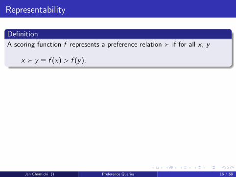
Representability
Definition
A scoring function f represents a preference relation � if for all x , y
x � y ≡ f (x) > f (y).
Necessary condition for representability
The preference relation � is a weak order.
Sufficient condition for representability
� is a weak order
the domain is countable or some continuity conditions are satisfied(studied in decision theory)
Jan Chomicki () Preference Queries 16 / 68

Not every WO can be represented using a scoring function
Lexicographic order in R × R
(x1, y1) �lo (x2, y2) ≡ x1 > x2 ∨ (x1 = x2 ∧ y1 > y2)
Proof1 Assume there is a real-valued function f such that
x �lo y ≡ f (x) > f (y).
2 For every x0, (x0, 1) �lo (x0, 0).
3 Thus f (x0, 1) > f (x0, 0).
4 Consider now x1 > x0.
5 Clearly f (x1, 1) > f (x1, 0) > f (x0, 1) > f (x0, 0).
6 So there are uncountably many nonempty disjoint intervals in R.
7 Each such interval contains a rational number: contradiction with thecountability of the set of rational numbers.
Jan Chomicki () Preference Queries 17 / 68

Not every WO can be represented using a scoring function
Lexicographic order in R × R
(x1, y1) �lo (x2, y2) ≡ x1 > x2 ∨ (x1 = x2 ∧ y1 > y2)
Proof
1 Assume there is a real-valued function f such thatx �lo y ≡ f (x) > f (y).
2 For every x0, (x0, 1) �lo (x0, 0).
3 Thus f (x0, 1) > f (x0, 0).
4 Consider now x1 > x0.
5 Clearly f (x1, 1) > f (x1, 0) > f (x0, 1) > f (x0, 0).
6 So there are uncountably many nonempty disjoint intervals in R.
7 Each such interval contains a rational number: contradiction with thecountability of the set of rational numbers.
Jan Chomicki () Preference Queries 17 / 68

Not every WO can be represented using a scoring function
Lexicographic order in R × R
(x1, y1) �lo (x2, y2) ≡ x1 > x2 ∨ (x1 = x2 ∧ y1 > y2)
Proof1 Assume there is a real-valued function f such that
x �lo y ≡ f (x) > f (y).
2 For every x0, (x0, 1) �lo (x0, 0).
3 Thus f (x0, 1) > f (x0, 0).
4 Consider now x1 > x0.
5 Clearly f (x1, 1) > f (x1, 0) > f (x0, 1) > f (x0, 0).
6 So there are uncountably many nonempty disjoint intervals in R.
7 Each such interval contains a rational number: contradiction with thecountability of the set of rational numbers.
Jan Chomicki () Preference Queries 17 / 68

Not every WO can be represented using a scoring function
Lexicographic order in R × R
(x1, y1) �lo (x2, y2) ≡ x1 > x2 ∨ (x1 = x2 ∧ y1 > y2)
Proof1 Assume there is a real-valued function f such that
x �lo y ≡ f (x) > f (y).
2 For every x0, (x0, 1) �lo (x0, 0).
3 Thus f (x0, 1) > f (x0, 0).
4 Consider now x1 > x0.
5 Clearly f (x1, 1) > f (x1, 0) > f (x0, 1) > f (x0, 0).
6 So there are uncountably many nonempty disjoint intervals in R.
7 Each such interval contains a rational number: contradiction with thecountability of the set of rational numbers.
Jan Chomicki () Preference Queries 17 / 68

Preference constructors [Kie02, KK02]
Good values
Prefer v ∈ S1 over v 6∈ S1.POS(Make,{mazda,vw})
Bad values
Prefer v 6∈ S1 over v ∈ S1.NEG(Make,{yugo})
Explicit preference
Preference encoded by a finitedirected graph.
EXP(Make,{(bmw,ford),...,(mazda,kia)})
Value comparison
Prefer larger/smaller values.HIGHEST(Year)
LOWEST(Price)
Distance
Prefer values closer to v0.
AROUND(Price,12K)
Jan Chomicki () Preference Queries 18 / 68

Preference constructors [Kie02, KK02]
Good values
Prefer v ∈ S1 over v 6∈ S1.
POS(Make,{mazda,vw})
Bad values
Prefer v 6∈ S1 over v ∈ S1.NEG(Make,{yugo})
Explicit preference
Preference encoded by a finitedirected graph.
EXP(Make,{(bmw,ford),...,(mazda,kia)})
Value comparison
Prefer larger/smaller values.HIGHEST(Year)
LOWEST(Price)
Distance
Prefer values closer to v0.
AROUND(Price,12K)
Jan Chomicki () Preference Queries 18 / 68

Preference constructors [Kie02, KK02]
Good values
Prefer v ∈ S1 over v 6∈ S1.POS(Make,{mazda,vw})
Bad values
Prefer v 6∈ S1 over v ∈ S1.NEG(Make,{yugo})
Explicit preference
Preference encoded by a finitedirected graph.
EXP(Make,{(bmw,ford),...,(mazda,kia)})
Value comparison
Prefer larger/smaller values.HIGHEST(Year)
LOWEST(Price)
Distance
Prefer values closer to v0.
AROUND(Price,12K)
Jan Chomicki () Preference Queries 18 / 68

Preference constructors [Kie02, KK02]
Good values
Prefer v ∈ S1 over v 6∈ S1.POS(Make,{mazda,vw})
Bad values
Prefer v 6∈ S1 over v ∈ S1.
NEG(Make,{yugo})
Explicit preference
Preference encoded by a finitedirected graph.
EXP(Make,{(bmw,ford),...,(mazda,kia)})
Value comparison
Prefer larger/smaller values.HIGHEST(Year)
LOWEST(Price)
Distance
Prefer values closer to v0.
AROUND(Price,12K)
Jan Chomicki () Preference Queries 18 / 68

Preference constructors [Kie02, KK02]
Good values
Prefer v ∈ S1 over v 6∈ S1.POS(Make,{mazda,vw})
Bad values
Prefer v 6∈ S1 over v ∈ S1.NEG(Make,{yugo})
Explicit preference
Preference encoded by a finitedirected graph.
EXP(Make,{(bmw,ford),...,(mazda,kia)})
Value comparison
Prefer larger/smaller values.HIGHEST(Year)
LOWEST(Price)
Distance
Prefer values closer to v0.
AROUND(Price,12K)
Jan Chomicki () Preference Queries 18 / 68

Preference constructors [Kie02, KK02]
Good values
Prefer v ∈ S1 over v 6∈ S1.POS(Make,{mazda,vw})
Bad values
Prefer v 6∈ S1 over v ∈ S1.NEG(Make,{yugo})
Explicit preference
Preference encoded by a finitedirected graph.
EXP(Make,{(bmw,ford),...,(mazda,kia)})
Value comparison
Prefer larger/smaller values.
HIGHEST(Year)
LOWEST(Price)
Distance
Prefer values closer to v0.
AROUND(Price,12K)
Jan Chomicki () Preference Queries 18 / 68

Preference constructors [Kie02, KK02]
Good values
Prefer v ∈ S1 over v 6∈ S1.POS(Make,{mazda,vw})
Bad values
Prefer v 6∈ S1 over v ∈ S1.NEG(Make,{yugo})
Explicit preference
Preference encoded by a finitedirected graph.
EXP(Make,{(bmw,ford),...,(mazda,kia)})
Value comparison
Prefer larger/smaller values.HIGHEST(Year)
LOWEST(Price)
Distance
Prefer values closer to v0.
AROUND(Price,12K)
Jan Chomicki () Preference Queries 18 / 68

Preference constructors [Kie02, KK02]
Good values
Prefer v ∈ S1 over v 6∈ S1.POS(Make,{mazda,vw})
Bad values
Prefer v 6∈ S1 over v ∈ S1.NEG(Make,{yugo})
Explicit preference
Preference encoded by a finitedirected graph.
EXP(Make,{(bmw,ford),...,(mazda,kia)})
Value comparison
Prefer larger/smaller values.HIGHEST(Year)
LOWEST(Price)
Distance
Prefer values closer to v0.
AROUND(Price,12K)
Jan Chomicki () Preference Queries 18 / 68

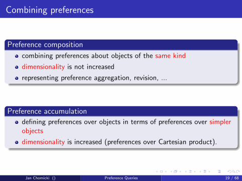
Combining preferences
Preference composition
combining preferences about objects of the same kind
dimensionality is not increased
representing preference aggregation, revision, ...
Preference accumulation
defining preferences over objects in terms of preferences over simplerobjects
dimensionality is increased (preferences over Cartesian product).
Jan Chomicki () Preference Queries 19 / 68

Combining preferences: composition
Boolean composition
x �∪ y ≡ x �1 y ∨ x �2 y
and similarly for ∩.
Prioritized composition
x �lex y ≡ x �1 y ∨ (y �1 x ∧ x �2 y).
Pareto composition
x �Par y ≡ (x �1 y ∧ y �2 x) ∨ (x �2 y ∧ y �1 x).
Jan Chomicki () Preference Queries 20 / 68

Combining preferences: composition
Boolean composition
x �∪ y ≡ x �1 y ∨ x �2 y
and similarly for ∩.
Prioritized composition
x �lex y ≡ x �1 y ∨ (y �1 x ∧ x �2 y).
Pareto composition
x �Par y ≡ (x �1 y ∧ y �2 x) ∨ (x �2 y ∧ y �1 x).
Jan Chomicki () Preference Queries 20 / 68

Combining preferences: composition
Boolean composition
x �∪ y ≡ x �1 y ∨ x �2 y
and similarly for ∩.
Prioritized composition
x �lex y ≡ x �1 y ∨ (y �1 x ∧ x �2 y).
Pareto composition
x �Par y ≡ (x �1 y ∧ y �2 x) ∨ (x �2 y ∧ y �1 x).
Jan Chomicki () Preference Queries 20 / 68

Combining preferences: composition
Boolean composition
x �∪ y ≡ x �1 y ∨ x �2 y
and similarly for ∩.
Prioritized composition
x �lex y ≡ x �1 y ∨ (y �1 x ∧ x �2 y).
Pareto composition
x �Par y ≡ (x �1 y ∧ y �2 x) ∨ (x �2 y ∧ y �1 x).
Jan Chomicki () Preference Queries 20 / 68

Preference composition
Preference relation �1
bmw
ford mazda
kia
Preference relation �2
bmw
ford
mazda
kia
Prioritized composition
bmw
ford
mazda
kia
Pareto composition
bmwford
mazdakia
Jan Chomicki () Preference Queries 21 / 68

Preference composition
Preference relation �1
bmw
ford mazda
kia
Preference relation �2
bmw
ford
mazda
kia
Prioritized composition
bmw
ford
mazda
kia
Pareto composition
bmwford
mazdakia
Jan Chomicki () Preference Queries 21 / 68

Preference composition
Preference relation �1
bmw
ford mazda
kia
Preference relation �2
bmw
ford
mazda
kia
Prioritized composition
bmw
ford
mazda
kia
Pareto composition
bmwford
mazdakia
Jan Chomicki () Preference Queries 21 / 68

Preference composition
Preference relation �1
bmw
ford mazda
kia
Preference relation �2
bmw
ford
mazda
kia
Prioritized composition
bmw
ford
mazda
kia
Pareto composition
bmwford
mazdakia
Jan Chomicki () Preference Queries 21 / 68

Preference composition
Preference relation �1
bmw
ford mazda
kia
Preference relation �2
bmw
ford
mazda
kia
Prioritized composition
bmw
ford
mazda
kia
Pareto composition
bmwford
mazdakia
Jan Chomicki () Preference Queries 21 / 68

Combining preferences: accumulation [Kie02]
Prioritized accumulation: �pr= (�1 & �2)
(x1, x2) �pr (y1, y2) ≡ x1 �1 y1 ∨ (x1 = y1 ∧ x2 �2 y2).
Pareto accumulation: �pa= (�1 ⊗ �2)
(x1, x2) �pa (y1, y2) ≡ (x1 �1 y1 ∧ x2 �2 y2) ∨ (x1 �1 y1 ∧ x2 �2 y2).
Properties
closure
associativity
commutativity of Pareto accumulation
Jan Chomicki () Preference Queries 22 / 68

Skylines
Skyline
Given single-attribute total preference relations �A1 , . . . ,�An for arelational schema R(A1, . . . ,An), the skyline preference relation �sky isdefined as
�sky=�A1 ⊗ �A2 ⊗ · · ·⊗ �An .
Unfolding the definition
(x1, . . . , xn) �sky (y1, . . . , yn) ≡∧i
xi �Aiyi ∧
∨i
xi �Aiyi .
Jan Chomicki () Preference Queries 23 / 68

Skyline in Euclidean space
Two-dimensional Euclidean space
(x1, x2) �sky (y1, y2) ≡ x1 ≥ y1 ∧ x2 > y2 ∨ x1 > y1 ∧ x2 ≥ y2
Skyline consists of �sky -maximal vectors
Jan Chomicki () Preference Queries 24 / 68

Skyline in Euclidean space
Two-dimensional Euclidean space
(x1, x2) �sky (y1, y2) ≡ x1 ≥ y1 ∧ x2 > y2 ∨ x1 > y1 ∧ x2 ≥ y2
Skyline consists of �sky -maximal vectors
Jan Chomicki () Preference Queries 24 / 68

Skyline in Euclidean space
Two-dimensional Euclidean space
(x1, x2) �sky (y1, y2) ≡ x1 ≥ y1 ∧ x2 > y2 ∨ x1 > y1 ∧ x2 ≥ y2
Skyline consists of �sky -maximal vectors
Jan Chomicki () Preference Queries 24 / 68

Skyline properties
Invariance
A skyline preference relation is unaffacted by scaling or shifting in anydimension.
Maxima
A skyline consists of the maxima of monotonic scoring functions.
Skyline is not a weak order
(2, 0) �sky (0, 2), (0, 2) �sky (1, 0), (2, 0) �sky (1, 0)
Jan Chomicki () Preference Queries 25 / 68

Skyline in SQL
Grouping
Designating attributes not used in comparisons (DIFF).
Example
SELECT * FROM Car
SKYLINE Price MIN,
Year MAX,
Make DIFF
Dynamic skylines
dimensions defined using dimension functions g1, . . . , gn
variable query point.
Jan Chomicki () Preference Queries 26 / 68

Skyline in SQL
Grouping
Designating attributes not used in comparisons (DIFF).
Example
SELECT * FROM Car
SKYLINE Price MIN,
Year MAX,
Make DIFF
Dynamic skylines
dimensions defined using dimension functions g1, . . . , gn
variable query point.
Jan Chomicki () Preference Queries 26 / 68

Skyline in SQL
Grouping
Designating attributes not used in comparisons (DIFF).
Example
SELECT * FROM Car
SKYLINE Price MIN,
Year MAX,
Make DIFF
Dynamic skylines
dimensions defined using dimension functions g1, . . . , gn
variable query point.
Jan Chomicki () Preference Queries 26 / 68

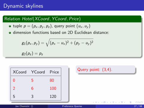
Dynamic skylines
Relation Hotel(XCoord ,YCoord ,Price)
tuple p = (px , py , pz), query point (ux , uy )
dimension functions based on 2D Euclidean distance:
g1(px , py ) =√
(px − ux)2 + (py − uy )2
g2(pz) = pz
XCoord YCoord Price
0 5 80
2 6 100
5 3 120
Query point: (3,4).
Jan Chomicki () Preference Queries 27 / 68

Combining scoring functions
Scoring functions can be combined using numerical operators.
Common scenario
scoring functions f1, . . . , fn
aggregate scoring function: F (t) = E (f1(t), . . . , fn(t))
linear scoring function: Σni=1αi fi
Numerical vs. logical combination
logical combination cannot be defined numerically
numerical combination cannot be defined logically (unless arithmeticoperators are available)
Jan Chomicki () Preference Queries 28 / 68

Part II
Preference Queries
Jan Chomicki () Preference Queries 29 / 68

Outline of Part II
2 Preference queriesRetrieving non-dominated elementsRewriting queries with winnowRetrieving Top-K elementsOptimizing Top-K queries
Jan Chomicki () Preference Queries 30 / 68

Winnow[Cho03]
Winnow
new relational algebra operator ω (other names: Best, BMO [Kie02])
retrieves the non-dominated (best) elements in a database relation
can be expressed in terms of other operators
Definition
Given a preference relation � and a database relation r :
ω�(r) = {t ∈ r | ¬∃t ′ ∈ r . t ′ � t}.
Notation: If a preference relation �C is defined using a formula C , thenwe write ωC (r), instead of ω�C
(r).
Skyline query
ω�sky (r) computes the set of maximal vectors in r (the skyline set).
Jan Chomicki () Preference Queries 31 / 68

Example of winnow
Relation Car(Make,Year ,Price)
Preference relation:
(m, y , p) �1 (m′, y ′, p′) ≡ y > y ′ ∨ (y = y ′ ∧ p < p′).
Make Year Price
mazda 2009 20K
ford 2009 15K
ford 2007 12K
Jan Chomicki () Preference Queries 32 / 68

Example of winnow
Relation Car(Make,Year ,Price)
Preference relation:
(m, y , p) �1 (m′, y ′, p′) ≡ y > y ′ ∨ (y = y ′ ∧ p < p′).
Make Year Price
mazda 2009 20K
ford 2009 15K
ford 2007 12K
Jan Chomicki () Preference Queries 32 / 68

Example of winnow
Relation Car(Make,Year ,Price)
Preference relation:
(m, y , p) �1 (m′, y ′, p′) ≡ y > y ′ ∨ (y = y ′ ∧ p < p′).
Make Year Price
mazda 2009 20K
ford 2009 15K
ford 2007 12K
Jan Chomicki () Preference Queries 32 / 68

Example of winnow
Relation Car(Make,Year ,Price)
Preference relation:
(m, y , p) �1 (m′, y ′, p′) ≡ y > y ′ ∨ (y = y ′ ∧ p < p′).
Make Year Price
mazda 2009 20K
ford 2009 15K
ford 2007 12K
Jan Chomicki () Preference Queries 32 / 68

Computing winnow using BNL [BKS01]
Require: SPO �, database relation r
1: initialize window W and temporary file F to empty2: repeat3: for every tuple t in the input do4: if t is dominated by a tuple in W then5: ignore t6: else if t dominates some tuples in W then7: eliminate them and insert t into W8: else if there is room in W then9: insert t into W
10: else11: add t to F12: end if13: end for14: output tuples from W that were added when F was empty15: make F the input, clear F16: until empty input
Jan Chomicki () Preference Queries 33 / 68

BNL in action
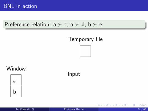
Preference relation: a � c, a � d, b � e.
Window
Temporary file
Input
Jan Chomicki () Preference Queries 34 / 68

BNL in action
Preference relation: a � c, a � d, b � e.
Window
Temporary file
Input
c,e,d,a,b
Jan Chomicki () Preference Queries 34 / 68

BNL in action
Preference relation: a � c, a � d, b � e.
Window
c
Temporary file
Input
e,d,a,b
Jan Chomicki () Preference Queries 34 / 68

BNL in action
Preference relation: a � c, a � d, b � e.
Window
c
e
Temporary file
Input
d,a,b
Jan Chomicki () Preference Queries 34 / 68

BNL in action
Preference relation: a � c, a � d, b � e.
Window
c
e
Temporary file
d
Input
a,b
Jan Chomicki () Preference Queries 34 / 68

BNL in action
Preference relation: a � c, a � d, b � e.
Window
a
e
Temporary file
d
Input
b
Jan Chomicki () Preference Queries 34 / 68

BNL in action
Preference relation: a � c, a � d, b � e.
Window
a
b
Temporary file
d
Input
Jan Chomicki () Preference Queries 34 / 68

BNL in action
Preference relation: a � c, a � d, b � e.
Window
a
b
Temporary file
Input
d
Jan Chomicki () Preference Queries 34 / 68
BNL in action
Preference relation: a � c, a � d, b � e.
Window
a
b
Temporary file
Input
Jan Chomicki () Preference Queries 34 / 68

Computing winnow with presorting
SFS: adding presorting step to BNL [CGGL03]
topologically sort the input:
if x dominates y , then x precedes y in the sorted inputwindow contains only winnow points and can be output after every pass
for skylines: sort the input using a monotonic scoring function, forexample
∏ki=1 xi .
LESS: integrating different techniques [GSG07]
adding an elimination filter to the first external sort pass
combining the last external sort pass with the first SFS pass
average running time: O(kn)
Jan Chomicki () Preference Queries 35 / 68

SFS in action
Preference relation: a � c, a � d, b � e.
Window
Temporary file
Input
Jan Chomicki () Preference Queries 36 / 68

SFS in action
Preference relation: a � c, a � d, b � e.
Window
Temporary file
Input
a,b,c,d,e
Jan Chomicki () Preference Queries 36 / 68

SFS in action
Preference relation: a � c, a � d, b � e.
Window
a
Temporary file
Input
b,c,d,e
Jan Chomicki () Preference Queries 36 / 68

SFS in action
Preference relation: a � c, a � d, b � e.
Window
a
b
Temporary file
Input
c,d,e
Jan Chomicki () Preference Queries 36 / 68

SFS in action
Preference relation: a � c, a � d, b � e.
Window
a
b
Temporary file
Input
d,e
Jan Chomicki () Preference Queries 36 / 68

SFS in action
Preference relation: a � c, a � d, b � e.
Window
a
b
Temporary file
Input
e
Jan Chomicki () Preference Queries 36 / 68

SFS in action
Preference relation: a � c, a � d, b � e.
Window
a
b
Temporary file
Input
Jan Chomicki () Preference Queries 36 / 68

Generalizations of winnow
Iterating winnow
ω0�(r) = ω�(r)
ωn+1� (r) = ω�(r −
⋃1≤i≤n ω
i�(r))
Ranking
Rank tuples by their minimum distance from a winnow tuple:
η�(r) = {(t, i) | t ∈ ωiC (r)}.
k-band
Return the tuples dominated by at most k tuples:
ω�(r) = {t ∈ r | #{t ′ ∈ r | t ′ � t} ≤ k}.
Jan Chomicki () Preference Queries 37 / 68

Preference SQL
The language
basic preference constructors
Pareto/prioritized accumulation
new SQL clause PREFERRING
groupwise preferences
implementation: translation to SQL
Winnow in Preference SQLSELECT * FROM Car
PREFERRING HIGHEST(Year)
CASCADE LOWEST(Price)
Jan Chomicki () Preference Queries 38 / 68

Algebraic laws [Cho03]
Commutativity of winnow with selection
If the formula
∀t1, t2.[α(t2) ∧ γ(t1, t2)]⇒ α(t1)
is valid, then for every r
σα(ωγ(r)) = ωγ(σα(r)).
Under the preference relation
(m, y , p) �C1 (m′, y ′, p′) ≡ y > y ′ ∧ p ≤ p′ ∨ y ≥ y ′ ∧ p < p′
the selection σPrice<20K commutes with ωC1 but σPrice>20K does not.
Jan Chomicki () Preference Queries 39 / 68

Other algebraic laws
Distributivity of winnow over Cartesian product
For every r1 and r2
ωC (r1 × r2) = ωC (r1)× r2
if C refers only to the attributes of r1.
Commutativity of winnow
If ∀t1, t2.[C1(t1, t2)⇒ C2(t1, t2)] is valid and �C1 and �C2 are SPOs, thenfor all finite instances r :
ωC1(ωC2(r)) = ωC2(ωC1(r)) = ωC2(r).
Jan Chomicki () Preference Queries 40 / 68

Semantic query optimization [Cho07b]
Using information about integrity constraints to:
eliminate redundant occurrences of winnow.
make more efficient computation of winnow possible.
Eliminating redundancy
Given a set of integrity constraints F , ωC is redundant w.r.t. F iff Fimplies the formula
∀t1, t2. R(t1) ∧ R(t2)⇒ t1 ∼C t2.
Jan Chomicki () Preference Queries 41 / 68

Integrity constraints
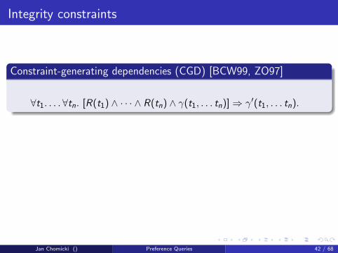
Constraint-generating dependencies (CGD) [BCW99, ZO97]
∀t1. . . .∀tn. [R(t1) ∧ · · · ∧ R(tn) ∧ γ(t1, . . . tn)]⇒ γ′(t1, . . . tn).
CGD entailment
Decidable by reduction to the validity of ∀-formulas in the constrainttheory (assuming the theory is decidable).
Jan Chomicki () Preference Queries 42 / 68
Integrity constraints
Constraint-generating dependencies (CGD) [BCW99, ZO97]
∀t1. . . .∀tn. [R(t1) ∧ · · · ∧ R(tn) ∧ γ(t1, . . . tn)]⇒ γ′(t1, . . . tn).
CGD entailment
Decidable by reduction to the validity of ∀-formulas in the constrainttheory (assuming the theory is decidable).
Jan Chomicki () Preference Queries 42 / 68

Top-K queries
Scoring functions
each tuple t in a relation has numeric scores f1(t), . . . , fm(t) assignedby numeric component scoring functions f1, . . . , fm
the aggregate score of t is F (t) = E (f1(t), . . . , fm(t)) where E is anumeric-valued expression
F is monotone if E (x1, . . . , xm) ≤ E (y1, . . . , ym) whenever xi ≤ yi forall i
Top-K queries
return K elements having top F -values in a database relation R
query expressed in an extension of SQL:
SELECT *
FROM R
ORDER BY F DESC
LIMIT K
Jan Chomicki () Preference Queries 43 / 68

Top-K queries
Scoring functions
each tuple t in a relation has numeric scores f1(t), . . . , fm(t) assignedby numeric component scoring functions f1, . . . , fm
the aggregate score of t is F (t) = E (f1(t), . . . , fm(t)) where E is anumeric-valued expression
F is monotone if E (x1, . . . , xm) ≤ E (y1, . . . , ym) whenever xi ≤ yi forall i
Top-K queries
return K elements having top F -values in a database relation R
query expressed in an extension of SQL:
SELECT *
FROM R
ORDER BY F DESC
LIMIT K
Jan Chomicki () Preference Queries 43 / 68

Top-K sets
Definition
Given a scoring function F and a database relation r , s is a Top-K set if:
s ⊆ r
|s| = min(K , |r |)∀t ∈ s. ∀t ′ ∈ r − s. F (t) ≥ F (t ′)
There may be more than one Top-K set: one is selectednon-deterministically.
Jan Chomicki () Preference Queries 44 / 68

Top-K sets
Definition
Given a scoring function F and a database relation r , s is a Top-K set if:
s ⊆ r
|s| = min(K , |r |)∀t ∈ s. ∀t ′ ∈ r − s. F (t) ≥ F (t ′)
There may be more than one Top-K set: one is selectednon-deterministically.
Jan Chomicki () Preference Queries 44 / 68

Example of Top-2
Relation Car(Make,Year ,Price)
component scoring functions:
f1(m, y , p) = (y − 2005)
f2(m, y , p) = (20000− p)
aggregate scoring function:F (m, y , p) = 1000 · f1(m, y , p) + f2(m, y , p)
Make Year Price Aggregate score
mazda 2009 20000 4000
ford 2009 15000 9000
ford 2007 12000 10000
Jan Chomicki () Preference Queries 45 / 68

Computing Top-K
Naive approaches
sort, output the first K -tuples
scan the input maintaining a priority queue of size K
...
Better approaches
the entire input does not need to be scanned...
... provided additional data structures are available
variants of the threshold algorithm
Jan Chomicki () Preference Queries 46 / 68

Threshold algorithm (TA)[FLN03]
Inputs
a monotone scoring function F (t) = E (f1(t), . . . , fm(t))
lists Si , i = 1, . . . ,m, each sorted on fi (descending) and representing adifferent ranking of the same set of objects
1 For each list Si in parallel, retrieve the current object w in sorted order:
(random access) for every j 6= i , retrieve vj = fj(w) from the list Sj
if d = E (v1, . . . , vm) is among the highest K scores seen so far,remember w and d (ties broken arbitrarily)
2 Thresholding:
for each i , wi is the last object seen under sorted access in Si
if there are already K top-K objects with score at least equal to thethreshold T = E (f1(w1), . . . , fm(wm)), return collected objects sortedby F and terminateotherwise, go to step 1.
Jan Chomicki () Preference Queries 47 / 68

TA in action
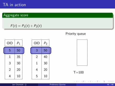
Aggregate score
F (t) = P1(t) + P2(t)
Priority queue
OID P1
5 50
1 35
3 30
2 20
4 10
OID P2
3 50
2 40
1 30
4 20
5 10
Jan Chomicki () Preference Queries 48 / 68
TA in action
Aggregate score
F (t) = P1(t) + P2(t)
Priority queue
T=100
OID P1
5 50
1 35
3 30
2 20
4 10
OID P2
3 50
2 40
1 30
4 20
5 10
Jan Chomicki () Preference Queries 48 / 68

TA in action
Aggregate score
F (t) = P1(t) + P2(t)
Priority queue
5:60
T=100
OID P1
5 50
1 35
3 30
2 20
4 10
OID P2
3 50
2 40
1 30
4 20
5 10
Jan Chomicki () Preference Queries 48 / 68

TA in action
Aggregate score
F (t) = P1(t) + P2(t)
Priority queue
3:80
5:60
T=100
OID P1
5 50
1 35
3 30
2 20
4 10
OID P2
3 50
2 40
1 30
4 20
5 10
Jan Chomicki () Preference Queries 48 / 68
TA in action
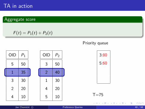
Aggregate score
F (t) = P1(t) + P2(t)
Priority queue
3:80
5:60
T=75
OID P1
5 50
1 35
3 30
2 20
4 10
OID P2
3 50
2 40
1 30
4 20
5 10
Jan Chomicki () Preference Queries 48 / 68

TA in action
Aggregate score
F (t) = P1(t) + P2(t)
Priority queue
3:80
1:65
5:60
T=75
OID P1
5 50
1 35
3 30
2 20
4 10
OID P2
3 50
2 40
1 30
4 20
5 10
Jan Chomicki () Preference Queries 48 / 68

TA in action
Aggregate score
F (t) = P1(t) + P2(t)
Priority queue
3:80
1:65
5:60
2:60
T=75
OID P1
5 50
1 35
3 30
2 20
4 10
OID P2
3 50
2 40
1 30
4 20
5 10
Jan Chomicki () Preference Queries 48 / 68

TA in databases
objects: tuples of a single relation r
single-attribute component scoring functions
sorted list access implemented through indexes
random access to all lists implemented by primary index access to rthat retrieves entire tuples
Jan Chomicki () Preference Queries 49 / 68

TA in databases
objects: tuples of a single relation r
single-attribute component scoring functions
sorted list access implemented through indexes
random access to all lists implemented by primary index access to rthat retrieves entire tuples
Jan Chomicki () Preference Queries 49 / 68

Optimizing Top-K queries [LCIS05]
Goals
integrating Top-K with relational query evaluation and optimization
replacing blocking by pipelining
Example
SELECT *
FROM Hotel h, Restaurant r, Museum mWHERE c1 AND c2 AND c3ORDER BY f1 + f2 + f3LIMIT K
Is there a better evaluation plan than materialize-then-sort?
Jan Chomicki () Preference Queries 50 / 68

Partial ranking of tuples
Model
set of component scoring functions P = {f1, . . . , fm} such thatfi (t) ≤ 1 for all t
aggregate scoring function F (t) = E (f1(t), . . . , fm(t))
how to rank intermediate tuples?
Ranking principle
Given P0 ⊆ P,
FP0(t) = E (g1(t), . . . , gm(t))
where
gi (t) =
fi (t) if fi ∈ P0
1 otherwise
Jan Chomicki () Preference Queries 51 / 68

Relations with rank
Rank-relation RP0
relation R
monotone aggregate scoring function F (the same for all relations)
set of component scoring functions P0 ⊆ P
order:
t1 >RP0t2 ≡ FP0(t1) > FP0(t2)
Jan Chomicki () Preference Queries 52 / 68

Relations with rank
Rank-relation RP0
relation R
monotone aggregate scoring function F (the same for all relations)
set of component scoring functions P0 ⊆ P
order:
t1 >RP0t2 ≡ FP0(t1) > FP0(t2)
Jan Chomicki () Preference Queries 52 / 68

Ranking intermediate results
Operators
rank operator µf : ranks tuples according to an additional componentscoring function f
standard relational algebra operators suitably extended to work onrank-relations
Operator Order
µf (RP0) t1 >µf (RP0) t2 ≡ FP0∪{f }(t1) > FP0∪{f }(t2)
RP1 ∩ SP2 t1 >RP1∩SP2 t2 ≡ FP1∪P2(t1) > FP1∪P2(t2)
Jan Chomicki () Preference Queries 53 / 68

Example
Query
SELECT *
FROM SORDER BY f1 + f2 + f3LIMIT 1
Unranked relation S
A f1 f2 f3
1 0.7 0.8 0.9
2 0.9 0.85 0.8
3 0.5 0.45 0.75
Rank-relation S{f1}
A F{f1}
2 2.9
1 2.7
3 2.5
Jan Chomicki () Preference Queries 54 / 68

Example
Query
SELECT *
FROM SORDER BY f1 + f2 + f3LIMIT 1
Unranked relation S
A f1 f2 f3
1 0.7 0.8 0.9
2 0.9 0.85 0.8
3 0.5 0.45 0.75
Rank-relation S{f1}
A F{f1}
2 2.9
1 2.7
3 2.5
Jan Chomicki () Preference Queries 54 / 68

Example
Query
SELECT *
FROM SORDER BY f1 + f2 + f3LIMIT 1
Unranked relation S
A f1 f2 f3
1 0.7 0.8 0.9
2 0.9 0.85 0.8
3 0.5 0.45 0.75
Rank-relation S{f1}
A F{f1}
2 2.9
1 2.7
3 2.5
Jan Chomicki () Preference Queries 54 / 68

Example
Query
SELECT *
FROM SORDER BY f1 + f2 + f3LIMIT 1
Unranked relation S
A f1 f2 f3
1 0.7 0.8 0.9
2 0.9 0.85 0.8
3 0.5 0.45 0.75
Rank-relation S{f1}
A F{f1}
2 2.9
1 2.7
3 2.5
Jan Chomicki () Preference Queries 54 / 68

Pipelined execution
A f1 f2 f3 F{f1}
2 0.9 0.85 0.8 2.9
1 0.7 0.8 0.9 2.7
3 0.5 0.45 0.75 2.5
IndexScanf1
A F{f1,f2}
2 2.75
1 2.5
3 1.95
µf2
A F{f1,f2,f3}
2 2.55
1 2.4
µf3
Jan Chomicki () Preference Queries 55 / 68

Pipelined execution
A f1 f2 f3 F{f1}
2 0.9 0.85 0.8 2.9
1 0.7 0.8 0.9 2.7
3 0.5 0.45 0.75 2.5
IndexScanf1
A F{f1,f2}
2 2.75
1 2.5
3 1.95
µf2
A F{f1,f2,f3}
2 2.55
1 2.4
µf3
Jan Chomicki () Preference Queries 55 / 68

Pipelined execution
A f1 f2 f3 F{f1}
2 0.9 0.85 0.8 2.9
1 0.7 0.8 0.9 2.7
3 0.5 0.45 0.75 2.5
IndexScanf1
A F{f1,f2}
2 2.75
1 2.5
3 1.95
µf2
A F{f1,f2,f3}
2 2.55
1 2.4
µf3
Jan Chomicki () Preference Queries 55 / 68

Pipelined execution
A f1 f2 f3 F{f1}
2 0.9 0.85 0.8 2.9
1 0.7 0.8 0.9 2.7
3 0.5 0.45 0.75 2.5
IndexScanf1
A F{f1,f2}
2 2.75
1 2.5
3 1.95
µf2
A F{f1,f2,f3}
2 2.55
1 2.4
µf3
Jan Chomicki () Preference Queries 55 / 68

Algebraic laws for rank-relation operators
Splitting for µ
R{f1,f2,...,fm} ≡ µf1(µf2(. . . (µfm(R)) . . .))
Commutativity of µ
µf1(µf2(RP0)) ≡ µf2(µf1(RP0))
Commutativity of µ with selection
σC (µf (RP0)) ≡ µf (σC (RP0))
Distributivity of µ over Cartesian product
µf (RP1 × SP2) ≡ µf (RP1)× SP2 if f refers only to the attributes of R.
Jan Chomicki () Preference Queries 56 / 68

Part III
Preference management
Jan Chomicki () Preference Queries 57 / 68

Outline of Part III
3 Preference managementPreference modification
Jan Chomicki () Preference Queries 58 / 68

Preference modification
Goal
Given a preference relation � and additional preference or indifferenceinformation I, construct a new preference relation �′ whose contentsdepend on � and I.
General postulates
fulfillment: the new information I should be completely incorporatedinto �′
minimal change: � should be changed as little as possible
closure:
order-theoretic properties of � should be preserved in �′ (SPO, WO)finiteness or finite representability of � should also be preserved in �′
Jan Chomicki () Preference Queries 59 / 68

Preference revision [Cho07a]
Setting
new information: revising preference relation �0
composition operator θ: union, prioritized or Pareto composition
composition eliminates (some) preference conflicts
additional assumptions: interval orders
�′= TC (�0 θ �) to guarantee SPO
VW , 2009
VW , 2008
VW , 2007
Kia, 2009
Kia, 2008
Kia, 2007
Jan Chomicki () Preference Queries 60 / 68

Preference contraction [MC08]
Setting
new information: contractor relation CON
�′: maximal subset of � disjoint with CON
VW , 2009
VW , 2008
VW , 2007
VW , 2006
VW , 2005
Jan Chomicki () Preference Queries 61 / 68

Preference contraction [MC08]
Setting
new information: contractor relation CON
�′: maximal subset of � disjoint with CON
VW , 2009
VW , 2008
VW , 2007
VW , 2006
VW , 2005
Jan Chomicki () Preference Queries 61 / 68

Preference contraction [MC08]
Setting
new information: contractor relation CON
�′: maximal subset of � disjoint with CON
VW , 2009
VW , 2008
VW , 2007
VW , 2006
VW , 2005
Jan Chomicki () Preference Queries 61 / 68

Preference contraction [MC08]
Setting
new information: contractor relation CON
�′: maximal subset of � disjoint with CON
VW , 2009
VW , 2008
VW , 2007
VW , 2006
VW , 2005
Jan Chomicki () Preference Queries 61 / 68

Preference contraction [MC08]
Setting
new information: contractor relation CON
�′: maximal subset of � disjoint with CON
VW , 2009
VW , 2008
VW , 2007
VW , 2006
VW , 2005
Jan Chomicki () Preference Queries 61 / 68

Substitutability [BGS06]
Setting
new information: set of indifference pairs
additional preferences are added to convert indifference to restrictedindifference
achieving object substitutability
VW , 2009
VW , 2008
VW , 2007
Kia, 2009
Kia, 2008
Kia, 2007
Jan Chomicki () Preference Queries 62 / 68

Substitutability [BGS06]
Setting
new information: set of indifference pairs
additional preferences are added to convert indifference to restrictedindifference
achieving object substitutability
VW , 2009
VW , 2008
VW , 2007
Kia, 2009
Kia, 2008
Kia, 2007
Jan Chomicki () Preference Queries 62 / 68

Substitutability [BGS06]
Setting
new information: set of indifference pairs
additional preferences are added to convert indifference to restrictedindifference
achieving object substitutability
VW , 2009
VW , 2008
VW , 2007
Kia, 2009
Kia, 2008
Kia, 2007
Jan Chomicki () Preference Queries 62 / 68

Substitutability [BGS06]
Setting
new information: set of indifference pairs
additional preferences are added to convert indifference to restrictedindifference
achieving object substitutability
VW , 2009
VW , 2008
VW , 2007
Kia, 2009
Kia, 2008
Kia, 2007
Jan Chomicki () Preference Queries 62 / 68

Substitutability [BGS06]
Setting
new information: set of indifference pairs
additional preferences are added to convert indifference to restrictedindifference
achieving object substitutability
VW , 2009
VW , 2008
VW , 2007
Kia, 2009
Kia, 2008
Kia, 2007
Jan Chomicki () Preference Queries 62 / 68

Part IV
Advanced topics
Jan Chomicki () Preference Queries 63 / 68

Outline of Part IV
Jan Chomicki () Preference Queries 64 / 68

Prospective research topics
Definability
Given a preference relation �C , how to construct a definition of a scoringfunction F representing �C , if such a function exists?
Extrinsic preference relations
Preference relations that are not fully defined by tuple contents:
x � y ≡ ∃n1, n2. Dissatisfied(x , n1) ∧ Dissatisfied(y , n2) ∧ n1 < n2.
Incomplete preferences
tuple scores and probabilities [SIC08, ZC08]
uncertain tuple scores
disjunctive preferences: a � b ∨ a � c
Jan Chomicki () Preference Queries 65 / 68

Preference modification
beyond revision and contraction: merging, arbitration,...
general parametric framework?
conflict resolution
Variations
preference and similarity: “find the objects similar to one of the bestobjects”
Applications
preference queries as decision components: workflows, event systems
personalization of query results
preference negotiation: applying contraction
Jan Chomicki () Preference Queries 66 / 68

Acknowledgments
Denis MindolinS lawek StaworkoXi Zhang
Jan Chomicki () Preference Queries 67 / 68

Jan Chomicki () Preference Queries 68 / 68

M. Baudinet, J. Chomicki, and P. Wolper.Constraint-Generating Dependencies.Journal of Computer and System Sciences, 59:94–115, 1999.Preliminary version in ICDT’95.
W-T. Balke, U. Guntzer, and W. Siberski.Exploiting Indifference for Customization of Partial Order Skylines.In International Database Engineering and Applications Symposium(IDEAS), pages 80–88, 2006.
S. Borzsonyi, D. Kossmann, and K. Stocker.The Skyline Operator.In IEEE International Conference on Data Engineering (ICDE), pages421–430, 2001.
J. Chomicki, P. Godfrey, J. Gryz, and D. Liang.Skyline with Presorting.In IEEE International Conference on Data Engineering (ICDE), 2003.Poster.
J. Chomicki.
Jan Chomicki () Preference Queries 68 / 68

Preference Formulas in Relational Queries.ACM Transactions on Database Systems, 28(4):427–466, December2003.
J. Chomicki.Database Querying under Changing Preferences.Annals of Mathematics and Artificial Intelligence, 50(1-2):79–109,2007.
J. Chomicki.Semantic optimization techniques for preference queries.Information Systems, 32(5):660–674, 2007.
R. Fagin, A. Lotem, and M. Naor.Optimal Aggregation Algorithms for Middleware.Journal of Computer and System Sciences, 66(4):614–656, 2003.
P. Godfrey, R. Shipley, and J. Gryz.Algorithms and Analyses for Maximal Vector Computation.VLDB Journal, 16:5–28, 2007.
W. Kießling.
Jan Chomicki () Preference Queries 68 / 68

Foundations of Preferences in Database Systems.In International Conference on Very Large Data Bases (VLDB), pages311–322, 2002.
W. Kießling and G. Kostler.Preference SQL - Design, Implementation, Experience.In International Conference on Very Large Data Bases (VLDB), pages990–1001, 2002.
C. Li, K. C-C. Chang, I.F. Ilyas, and S. Song.RankSQL: Query Algebra and Optimization for Relational Top-kQueries.In ACM SIGMOD International Conference on Management of Data,pages 131–142, 2005.
D. Mindolin and J. Chomicki.Maximal Contraction of Preference Relations.In National Conference on Artificial Intelligence, pages 492–497, 2008.
M.A. Soliman, I.F. Ilyas, and K. C-C. Chang.Probabilistic Top-k and Ranking-Aggregate Queries.
Jan Chomicki () Preference Queries 68 / 68

ACM Transactions on Database Systems, 33(3):13:1–13:54, 2008.
X. Zhang and J. Chomicki.On the Semantics and Evaluation of Top-k Queries in ProbabilisticDatabases.In International Workshop on Database Ranking (DBRank). IEEEComputer Society (ICDE Workshops), 2008.
X. Zhang and Z. M. Ozsoyoglu.Implication and Referential Constraints: A New Formal Reasoning.IEEE Transactions on Knowledge and Data Engineering,9(6):894–910, 1997.
Jan Chomicki () Preference Queries 68 / 68