FOUNDATIONS OF ALGEBRAIC GEOMETRY CLASS...

FOUNDATIONS OF ALGEBRAIC GEOMETRY CLASS 21

RAVI VAKIL

CONTENTS

1. Nonsingularity (“smoothness”) of Noetherian schemes 12. The Zariski tangent space 23. The local dimension is at most the dimension of the tangent space 6

This class will meet 8:40-9:55. Please be sure to be on the e-mail list so I can warnyou which days class will take place.

Welcome back! Where we’re going this quarter: last quarter, we established the objectsof study: varieties or schemes. This quarter we’ll be mostly concerned with importantmeans of studying them: vector bundles quasicoherent sheaves and cohomology thereof.As a punchline for this quarter, I hope to say a lot of things about curves (Riemann sur-faces) at the end of the quarter. However, in keeping with the attitude of last quarter, mygoal isn’t to make a beeline for the punchline. Instead we’ll have a scorched-earth policyand try to cover everything between here and there relatively comprehensively. We startwith smoothness nonsingularity of schemes. Then vector bundles locally free sheaves,quasicoherent sheaves and coherent sheaves. Then to line bundles invertible sheaves,and divisors. Then we’ll interpret these for projective schemes in terms of graded mod-ules. We’ll investigate pushing forward and pulling back quasicoherent sheaves. We’llconstruct schemes using these notions, and for example define the notion of a projectivemorphism. We’ll study differentials (e.g. the tangent bundle of smooth schemes, but alsofor singular things). Then we’ll discuss cohomology (both Cech cohomology and derivedfunctor cohomology). Then curves! The punch line for today: Spec Z is a smooth nonsin-gular curve.

1. NONSINGULARITY (“SMOOTHNESS”) OF NOETHERIAN SCHEMES

One natural notion we expect to see for geometric spaces is the notion of when anobject is “smooth”. In algebraic geometry, this notion, called nonsingularity (or regularity,although we won’t use this term) is easy to define but a bit subtle in practice. We will soondefine what it means for a scheme to be nonsingular (or regular) at a point. A point thatis not nonsingular is (not surprisingly) called singular (“not smooth”). A scheme is saidnonsingular if all its points are nonsingular, and singular if one of its points is singular.

Date: Friday, January 11, 2008.

1

The notion of nonsingularity is less useful than you might think. Grothendieck taughtus that the more important notions are properties of morphisms, not of objects, and thereis indeed a “relative notion” that applies to a morphism of schemes f : X → Y that is muchbetter-behaved (corresponding to the notion of submersion in differential geometry). Forthis reason, the word “smooth” is reserved for these morphisms. We will discuss smoothmorphisms in the spring quarter. However, nonsingularity is still useful, especially in(co)dimension 1, and we shall discuss this case (of discrete valuation rings) next day.

2. THE ZARISKI TANGENT SPACE

We begin by defining the notion of the tangent space of a scheme at a point. It willbehave like the tangent space you know and love at “smooth” points, but will also makesense at other points. In other words, geometric intuition at the smooth points guides thedefinition, and then the definition guides the algebra at all points, which in turn lets usrefine our geometric intuition.

This definition is short but surprising. The main difficulty is convincing yourself thatit deserves to be called the tangent space. I’ve always found this tricky to explain, andthat is because we want to show that it agrees with our intuition; but unfortunately, ourintuition is worse than we realize. So I’m just going to define it for you, and later try toconvince you that it is reasonable.

Suppose p is a prime ideal of a ring A, so [p] is a point of Spec A. Then [pAp] is a pointof the scheme Spec Ap. For convenience, we let m := pAp ⊂ Ap =: B. Let k = B/m be theresidue field. Then m/m2 is a vector space over the residue field k: it is an B-module, andelements of m acts like 0. This is defined to be the Zariski cotangent space. The dual isthe Zariski tangent space. Elements of the Zariski cotangent space are called cotangentvectors or differentials; elements of the tangent space are called tangent vectors.

Note that this definition is intrinsic. It doesn’t depend on any specific description ofthe ring itself (such as the choice of generators over a field k, which is equivalent to thechoice of embedding in affine space). Notice that in some sense, the cotangent space ismore algebraically natural than the tangent space. There is a moral reason for this: thecotangent space is more naturally determined in terms of functions on a space, and weare very much thinking about schemes in terms of “functions on them”. This will comeup later.

I’ll give two of plausibility arguments that this is a reasonable definition. Hopefullyone will catch your fancy.

In differential geometry, the tangent space at a point is sometimes defined as the vectorspace of derivations at that point. A derivation is a function that takes in functions nearthe point that vanish at the point, and gives elements of the field k, and satisfies theLeibniz rule

(fg) ′ = f ′g + g ′f.

Translation: a derivation is a map m → k. But m2→ 0, as if f(p) = g(p) = 0, then

(fg) ′(p) = f ′(p)g(p) + g ′(p)f(p) = 0.

2

Thus we have a map m/m2→ k, i.e. an element of (m/m2)∨.

2.A. EXERCISE. Check that this is reversible, i.e. that any map m/m2→ k gives a deriva-

tion. In other words, verify that the Leibniz rule holds.

Here is a second vaguer motivation that this definition is plausible for the cotangentspace of the origin of A

n. Functions on An should restrict to a linear function on the

tangent space. What function does x2 + xy + x + y restrict to “near the origin”? Youwill naturally answer: x + y. Thus we “pick off the linear terms”. Hence m/m2 are thelinear functionals on the tangent space, so m/m2 is the cotangent space. In particular,you should picture functions vanishing at a point (lying in m) as giving functions on thetangent space in this obvious a way.

2.1. Old-fashioned example. Here is an example to help tie this down to earth. Computingthe Zariski-tangent space is actually quite hands-on, because you can compute it just asyou did when you learned multivariable calculus. In A

3, we have a curve cut out byx + y + z2 + xyz = 0 and x − 2y + z + x2y2z3 = 0. (You know enough to check thatthis is a curve, but it is not important to do so.) What is the tangent line near the origin?(Is it even smooth there?) Answer: the first surface looks like x + y = 0 and the secondsurface looks like x − 2y + z = 0. The curve has tangent line cut out by x + y = 0 andx − 2y + z = 0. It is smooth (in the analytic sense). In multivariable calculus, the studentsdo a page of calculus to get the answer, because we aren’t allowed to tell them to just pickout the linear terms.

Let’s make explicit the fact that we are using. If A is a ring, m is a maximal ideal, andf ∈ m is a function vanishing at the point [m] ∈ Spec A, then the Zariski tangent space ofSpec A/(f) at m is cut out in the Zariski tangent space of Spec A (at m) by the single linearequation f (mod m2). The next exercise will force you think this through.

2.B. IMPORTANT EXERCISE (“KRULL’S PRINCIPAL IDEAL THEOREM FOR THE ZARISKITANGENT SPACE”). Suppose A is a ring, and m a maximal ideal. If f ∈ m, show that theZariski tangent space of A/f is cut out in the Zariski tangent space of A by f (mod m2).(Note: we can quotient by f and localize at m in either order, as quotienting and localizing“commute”.) Hence the dimension of the Zariski tangent space of Spec A at [m] is thedimension of the Zariski tangent space of Spec A/(f) at [m], or one less.

Here is another example to see this principle in action: x + y + z2 = 0 and x + y +

x2 + y4 + z5 = 0 cuts out a curve, which obviously passes through the origin. If I askedmy multivariable calculus students to calculate the tangent line to the curve at the origin,they would do a reams of calculations which would boil down to picking off the linearterms. They would end up with the equations x + y = 0 and x + y = 0, which cuts outa plane, not a line. They would be disturbed, and I would explain that this is becausethe curve isn’t smooth at a point, and their techniques don’t work. We on the other handbravely declare that the cotangent space is cut out by x + y = 0, and (will soon) definethis as a singular point. (Intuitively, the curve near the origin is very close to lying in the

3

plane x + y = 0.) Notice: the cotangent space jumped up in dimension from what it was“supposed to be”, not down. We’ll see that this is not a coincidence soon, in Theorem 3.1.

Here is a nice consequence of the notion of Zariski tangent space.

2.2. Problem. Consider the ring A = k[x, y, z]/(xy−z2). Show that (x, z) is not a principalideal.

As dim A = 2 (by Krull’s Principal Ideal Theorem), and A/(x, z) ∼= k[y] has dimension1, we see that this ideal is height 1 (as codimension is the difference of dimensions forfinitely generated k-domains). Our geometric picture is that Spec A is a cone (we candiagonalize the quadric as xy− z2 = ((x+y)/2)2 −((x−y)/2)2 − z2, at least if char k 6= 2),and that (x, z) is a ruling of the cone. (See Figure 1 for a sketch.) This suggests that welook at the cone point.

FIGURE 1. V(x, z) ⊂ Spec k[x, y, z]/(xy − z2) is a ruling on a cone; (x, z)2 isnot (x, z)-primary.

Solution. Let m = (x, y, z) be the maximal ideal corresponding to the origin. ThenSpec A has Zariski tangent space of dimension 3 at the origin, and Spec A/(x, z) has Zariskitangent space of dimension 1 at the origin. But Spec A/(f) must have Zariski tangentspace of dimension at least 2 at the origin by Exercise 2.B.

2.C. EXERCISE. Show that (x, z) ⊂ k[w, x, y, z]/(wz − xy) is a codimension 1 ideal that isnot principal. (See Figure 2 for a sketch.)

2.3. Morphisms and tangent spaces. Suppose f : X → Y, and f(p) = q. Then if wewere in the category of manifolds, we would expect a tangent map, from the tangent

4

FIGURE 2. The ruling V(x, z) on V(wz − xy) ⊂ P3.

space of p to the tangent space at q. Indeed that is the case; we have a map of stalksOY,q → OX,p, which sends the maximal ideal of the former n to the maximal ideal of thelatter m (we have checked that this is a “local morphism” when we briefly discussed local-ringed spaces). Thus n2

→ m2, from which n/n2→ m/m2, from which we have a natural

map (m/m2)∨→ (n/n2)∨. This is the map from the tangent space of p to the tangent space

at q that we sought.

Here are some exercises to give you practice with the Zariski tangent space.

2.D. USEFUL EXERCISE (THE JACOBIAN CRITERION FOR COMPUTING THE ZARISKI TAN-GENT SPACE). Suppose k is an algebraically closed field, and X is a finite type k-scheme.Then locally it is of the form Spec k[x1, . . . , xn]/(f1, . . . , fr). Show that the Zariski tangentspace at the closed point p (with residue field k, by the Nullstellensatz) is given by thecokernel of the Jacobian map kr

→ kn given by the Jacobian matrix

(1) J =

∂f1

∂x1(p) · · · ∂fr

∂x1(p)

... . . . ...∂f1

∂xn(p) · · · ∂fr

∂xn(p)

.

(This is just making precise our example of a curve in A3 cut out by a couple of equations,

where we picked off the linear terms, see Example 2.1 .) You might be alarmed: whatdoes ∂f

∂x1mean?! Do you need deltas and epsilons? No! Just define derivatives formally,

e.g.∂

∂x1

(x21 + x1x2 + x2

2) = 2x1 + x2.

(Hint: Do this first when p is the origin, and consider linear terms, just as in Example 2.1.Note for future reference that you have not yet used the algebraic closure of k. Then inthe general case (with k algebraically closed), “translate p to the origin.”

5

2.E. LESS IMPORTANT EXERCISE (“HIGHER-ORDER DATA”). In an earlier exercise, youcomputed the equations cutting out the three coordinate axes of A

3k. (Call this scheme X.)

Your ideal should have had three generators. Show that the ideal can’t be generated byfewer than three elements. (Hint: working modulo m = (x, y, z) won’t give any usefulinformation, so work modulo m2.)

2.F. EXERCISE. Suppose X is a k-scheme. Describe a natural bijection Mork(Spec k[ε]/(ε2), X)to the data of a point with residue field is k, necessarily a closed point.

2.G. EXERCISE. Find the dimension of the Zariski tangent space at the point [(2, x)] ofZ[2i] ∼= Z[x]/(x2 + 4). Find the dimension of the Zariski tangent space at the point [(2, x)]

of Z[√

−2] ∼= Z[x]/(x2 + 2).

3. THE LOCAL DIMENSION IS AT MOST THE DIMENSION OF THE TANGENT SPACE

We are ready to define nonsingularity. The key idea is contained in the title of thissection.

3.1. Theorem. — Suppose (A, m) is a Noetherian local ring. Then dim A ≤ dimk m/m2.

If equality holds, we say that A is a regular local ring. If a Noetherian ring A is regularat all of its primes, we say that A is a regular ring.

A locally Noetherian scheme X is regular or nonsingular at a point p if the local ringOX,p is regular. It is singular at the point otherwise. A scheme is regular or nonsingularif it is regular at all points. It is singular otherwise (i.e. if it is singular at at least one point).

Proof of Theorem 3.1: Note that m is finitely generated (as A is Noetherian), so m/m2 isa finitely generated (A/m = k)-module, hence finite-dimensional. Say dimk m/m2 = n.Choose a basis of m/m2, and lift them to elements f1, . . . , fn of m. Then by Nakayama’slemma (version 4), (f1, . . . , fn) = m.

We need here one fancy fact that I forgot to say last quarter. Krull’s Principal IdealTheorem states that the codimension of any irreducible component of the locus cut out byone equation is at most one. There is a generalization to an arbitrary number of equations:if A is a Noetherian ring, then any irreducible component of V(f1, . . . , fn) has codimensionat most n. The proof isn’t much harder than Krull, but I haven’t given it to you. Sorry!You can read a proof in Eisenbud (Theorem 10.2, p. 235).

3.A. EXERCISE. Prove this if A is an irreducible variety over a field. (Hint: this isn’t thathard. Use the fact that codimension is the difference of dimensions in this happy case.)

6

In our case, V((f1, . . . , fn)) = V(m) is just the point [m], so the codimension of m isat most n. Thus the longest chain of prime ideals contained in m is at most n + 1. Butthis is also the longest chain of prime ideals in A (as m is the unique maximal ideal), son ≥ dim A. �

3.B. EXERCISE. Show that if A is a Noetherian local ring, then A has finite dimension.(Noetherian rings in general could have infinite dimension, as we saw in an earlier exer-cise.)

In the case of finite type schemes over an algebraically closed field k, the Jacobian crite-rion (Exercise 2.D) gives a hands-on method for checking for singularity at closed points.

3.C. EXERCISE. Suppose k is algebraically closed. Show that the singular closed points ofthe hypersurface f(x1, . . . , xn) = 0 in A

nk are given by the equations f = ∂f

∂x1= · · · = ∂f

∂xn=

0.

3.D. EXERCISE. Suppose k is algebraically closed. Show that A1k and A

2k are nonsingular.

(Make sure to check nonsingularity at the non-closed points! Fortunately you know whatall the points of A

2k are; this is trickier for A

3k.) Show that P

1k and P

2k are nonsingular. (This

holds even if k isn’t algebraically closed, and in higher dimension.)

Let’s apply this technology to an arithmetic situation.

3.E. EASY EXERCISE. Show that Spec Z is a nonsingular curve.

Here are some fun comments: What is the derivative of 35 at the prime 5? Answer: 35

(mod 25), so 35 has the same “slope” as 10. What is the derivative of 9, which doesn’tvanish at 5? Answer: the notion of derivative doesn’t apply there. You’d think that you’dwant to subtract its value at 5, but you can’t subtract “4 (mod 5)” from the integer 9. Also,35 (mod 25) you might think you want to restate as 7 (mod 5), by dividing by 5, but that’smorally wrong — you’re dividing by a particular choice of generator 5 of the maximalideal of Z5 (the 5-adics); in this case, one appears to be staring you in the face, but ingeneral that won’t be true. Follow-up fun: you can talk about the derivative of a functiononly for functions vanishing at a point. And you can talk about the second derivative of afunction only for functions that vanish, and whose first derivative vanishes. For example,75 has second derivative 75 (mod 125) at 5. It’s pretty flat.

3.F. EXERCISE. (This exercise is for those who know about the primes of the Gaussianintegers Z[i].) Note that Z[i] is dimension 1, as Z[x] has dimension 2 (problem set exercise),and is a domain, and x2 + 1 is not 0, so Z[x]/(x2 + 1) has dimension 1 by Krull’s PrincipalIdeal Theorem. Show that Spec Z[i] is a nonsingular curve.

3.G. EXERCISE. Show that there is one singular point of Spec Z[5i], and describe it.

7

Let’s return to more geometric examples.

3.H. EXERCISE (THE EULER TEST FOR PROJECTIVE HYPERSURFACES). There is an analo-gous Jacobian criterion for hypersurfaces f = 0 in P

nk . Suppose k is algebraically closed.

Show that the singular closed points correspond to the locus f = ∂f∂x1

= · · · = ∂f∂xn

= 0. Ifthe degree of the hypersurface is not divisible by the characteristic of any of the residuefields (e.g. if we are working over a field of characteristic 0), show that it suffices to check∂f

∂x1= · · · = ∂f

∂xn= 0. (Hint: show that f lies in the ideal ( ∂f

∂x1, . . . , ∂f

∂xn)). (Fact: this will give

the singular points in general, not just the closed points. I don’t want to prove this, and Iwon’t use it.)

3.I. EXERCISE. Suppose that k is algebraically closed. Show that y2z = x3 − xz2 in P2k is

an irreducible nonsingular curve. (This is for practice.) Warning: I didn’t say char k = 0,so be careful when using the Euler test.

3.J. EXERCISE. Find all the singular closed points of the following plane curves. Here wework over an algebraically closed field.

(a) y2 = x2 + x3. This is called a node.(b) y2 = x3. This is called a cusp.(c) y2 = x4. This is called a tacnode.

(I haven’t given a precise definition of a node, etc.)

3.K. EXERCISE. Show that the twisted cubic Proj k[w, x, y, z]/(wz − xy, wy − x2, xz − y2)is nonsingular. (You can do this by using the fact that it is isomorphic to P

1. I’d prefer youto do this with the explicit equations, for the sake of practice.)

E-mail address: [email protected]

8


RAVI VAKIL

CONTENTS

1. Discrete valuation rings: Dimension 1 Noetherian regular local rings 1

Last day, we discussed the Zariski tangent space, and saw that it was often quite com-putable. We proved the key inequality dim A ≤ dimk m/m2 for Noetherian local rings(A, m). When equality holds, we said that the ring was regular (or nonsingular), and wedefined the notion of (non)singularity for locally Noetherian schemes.

1. DISCRETE VALUATION RINGS: DIMENSION 1 NOETHERIAN REGULAR LOCAL RINGS

The case of dimension 1 is important, because if you understand how primes behavethat are separated by dimension 1, then you can use induction to prove facts in arbitrarydimension. This is one reason why Krull’s Principal Ideal Theorem is so useful.

A dimension 1 Noetherian regular local ring can be thought of as a “germ of a smoothcurve” (see Figure 1). Two examples to keep in mind are k[x](x) = {f(x)/g(x) : x 6 | g(x)}and Z(5) = {a/b : 5 6 | b}.

FIGURE 1. A germ of a curve

The purpose of this section is to give a long series of equivalent definitions of theserings. We will eventually have seven equivalent definitions, (a) through (g).

1.1. Theorem. — Suppose (A, m) is a Noetherian local ring of dimension 1. Then the followingare equivalent.

(a) (A, m) is regular.(b) m is principal.

Date: Monday, January 14, 2008.

1

Here is why (a) implies (b). If A is regular, then m/m2 is one-dimensional. Choose anyelement t ∈ m − m2. Then t generates m/m2, so generates m by Nakayama’s lemma. Wecall such an element a uniformizer. Warning: we need to know that m is finitely generatedto invoke Nakayama — but fortunately we do, thanks to the Noetherian hypothesis.

Conversely, if m is generated by one element t over A, then m/m2 is generated by oneelement t over A/m = k. Note that t /∈ m2, as otherwise m = m2 and hece m = 0 byNakayama’s Lemma. �

We will soon use a useful fact, and we may as well prove it in much more generalitythan we need, because the proof is so short.

1.2. Proposition. — If (A, m) is a Noetherian local ring, then ∩imi = 0.

The geometric intuition for this is that any function that is analytically zero at a point(vanishes to all orders) actually vanishes at that point.

It is tempting to argue that m(∩imi) = ∩im

i, and then to use Nakayama’s lemma toargue that ∩im

i = 0. Unfortunately, it is not obvious that this first equality is true: productdoes not commute with infinite intersections in general.

Proof. Let I = ∩imi. We wish to show that I ⊂ mI; then as mI ⊂ I, we have I = mI, and

hence by Nakayama’s Lemma, I = 0. Fix a primary decomposition of mI. It suffices toshow that q contains I for any q in this primary decomposition, as then I is contained inall the primary ideals in the decomposition of mI, and hence mI. Let p =

√q.

If p 6= m, then choose x ∈ m − p. Now x is not nilpotent in A/q, and hence is not azero-divisor. (Recall that q is primary if and only if in A/q, each zero-divisor is nilpotent.)But xI ⊂ mI ⊂ q, so I ⊂ q.

On the other hand, if p = m, then as m is finitely generated, and each generator is in√q = m, there is some a such that ma ⊂ q. But I ⊂ ma, so we are done. �

1.3. Proposition. — Suppose (A, m) is a Noetherian regular local ring of dimension 1 (i.e.satisfying (a) above). Then A is an integral domain.

Proof. Suppose xy = 0, and x, y 6= 0. Then by Proposition 1.2, x ∈ mi \mi+1 for some i ≥ 0,so x = ati for some a /∈ m. Similarly, y = btj for some j ≥ 0 and b /∈ m. As a, b /∈ m, a andb are invertible. Hence xy = 0 implies ti+j = 0. But as nilpotents don’t affect dimension,(1) dim A = dim A/(t) = dim A/m = dim k = 0,

contradicting dim A = 1. �

1.4. Theorem. — Suppose (A, m) is a Noetherian local ring of dimension 1. Then (a) and (b) areequivalent to:

2

(c) all ideals are of the form mn or 0.

Proof. Assume (a): suppose (A, m, k) is a Noetherian regular local ring of dimension 1.Then I claim that mn 6= mn+1 for any n. Otherwise, by Nakayama’s lemma, mn = 0, fromwhich tn = 0. But A is a domain, so t = 0, from which A = A/m is a field, which can’thave dimension 1, contradiction.

I next claim that mn/mn+1 is dimension 1. Reason: mn = (tn). So mn is generated asas a A-module by one element, and mn/(mmn) is generated as a (A/m = k)-module by 1

element (non-zero by the previous paragraph), so it is a one-dimensional vector space.

So we have a chain of ideals A ⊃ m ⊃ m2 ⊃ m3 ⊃ · · · with ∩mi = (0) (Proposition 1.2).We want to say that there is no room for any ideal besides these, because “each pair is“separated by dimension 1”, and there is “no room at the end”. Proof: suppose I ⊂ A isan ideal. If I 6= (0), then there is some n such that I ⊂ mn but I 6⊂ mn+1. Choose someu ∈ I − mn+1. Then (u) ⊂ I. But u generates mn/mn+1, hence by Nakayama it generatesmn, so we have mn ⊂ I ⊂ mn, so we are done. Conclusion: in a Noetherian local ring ofdimension 1, regularity implies all ideals are of the form mn or (0).

We now show that (c) implies (a). Assume (a) is false: suppose we have a dimension1 Noetherian local domain that is not regular, so m/m2 has dimension at least 2. Chooseany u ∈ m − m2. Then (u, m2) is an ideal, but m ( (u, m2) ( m2. �

1.A. EASY EXERCISE. Suppose (A, m) is a Noetherian dimension 1 local ring. Show that(a)–(c) above are equivalent to:

(d) A is a principal ideal domain.

1.5. Discrete valuation rings. We next define the notion of a discrete valuation ring.Suppose K is a field. A discrete valuation on K is a surjective homomorphism v : K∗

→ Z(homomorphism: v(xy) = v(x) + v(y)) satisfying

v(x + y) ≥ min(v(x), v(y))

except if x + y = 0 (in which case the left side is undefined). (Such a valuation is callednon-archimedean, although we will not use that term.) It is often convenient to say v(0) =∞. More generally, a valuation is a surjective homomorphism v : K∗

→ G to a totallyordered group G, although this isn’t so important to us. (Not every valuation is discrete.Consider the ring of Puisseux series over a field k, K = ∪n≥1k((x1/n)), with v : K∗

→ Q

given by v(xq) = q.)

Examples.

(i) (the 5-adic valuation) K = Q, v(r) is the “power of 5 appearing in r”, e.g. v(35/2) = 1,v(27/125) = −3.

(ii) K = k(x), v(f) is the “power of x appearing in f.”

3

(iii) K = k(x), v(f) is the negative of the degree. This is really the same as (ii), with x

replaced by 1/x.

Then 0 ∪ {x ∈ K∗ : v(x) ≥ 0} is a ring, which we denote Ov. It is called the valuationring of v.

1.B. EXERCISE. Describe the valuation rings in the three examples above. (You will noticethat they are familiar-looking dimension 1 Noetherian local rings. What a coincidence!)

1.C. EXERCISE. Show that 0 ∪ {x ∈ K∗ : v(x) ≥ 1} is the unique maximal ideal of thevaluation ring. (Hint: show that everything in the complement is invertible.) Thus thevaluation ring is a local ring.

An integral domain A is called a discrete valuation ring (or DVR) if there exists adiscrete valuation v on its fraction field K = FF(A) for which Ov = A.

Now if A is a Noetherian regular local ring of dimension 1, and t is a uniformizer (agenerator of m as an ideal, or equivalently of m/m2 as a k-vector space) then any non-zeroelement r of A lies in some mn − mn+1, so r = tnu where u is a unit (as tn generates mn

by Nakayama, and so does r), so FF(A) = At = A[1/t]. So any element of FF(A) can bewritten uniquely as utn where u is a unit and n ∈ Z. Thus we can define a valuationv(utn) = n.

1.D. EXERCISE. Show that v is a discrete valuation.

Thus (a)–(d) implies (e).

Conversely, suppose (A, m) is a discrete valuation ring.

1.E. EXERCISE. Show that (A, m) is a Noetherian regular local ring of dimension 1. (Hint:Show that the ideals are all of the form (0) or In = {r ∈ A : v(r) ≥ n}, and I1 is the onlyprime of the second sort. Then we get Noetherianness, and dimension 1. Show that I1/I2

is generated by the image of any element of I1 − I2.)

Hence we have proved:

1.6. Theorem. — An integral domain A is a Noetherian local ring of dimension 1 satisfying(a)–(d) if and only if

(e) A is a discrete valuation ring.

1.F. EXERCISE. Show that there is only one discrete valuation on a discrete valuation ring.

4

Thus any Noetherian regular local ring of dimension 1 comes with a unique valuationon its fraction field. If the valuation of an element is n > 0, we say that the element has azero of order n. If the valuation is −n < 0, we say that the element has a pole of order n.We’ll come back to this shortly, after dealing with (f) and (g).

1.7. Theorem. — Suppose (A, m) is a Noetherian local ring of dimension 1. Then (a)–(e) areequivalent to:

(f) A is a unique factorization domain,(g) A is integrally closed in its fraction field K = FF(A).

Proof. (a)–(e) clearly imply (f), because we have the following stupid unique factorization:each non-zero element of r can be written uniquely as utn where n ∈ Z≥0 and u is a unit.Also, (f) implies (b), by an earlier easy Proposition, that in a unique factorization domainall codimension 1 prime ideals are principal. (In fact, we could just have (b) ⇐⇒ (f) fromthe harder Proposition we proved, which showed that this property characterizes uniquefactorization domains.)

(f) implies (g), because unique factorization domains are integrally closed in their frac-tion fields (an earlier exercise).

It remains to check that (g) implies (a)–(e). We’ll show that (g) implies (b).

Suppose (A, m) is a Noetherian local domain of dimension 1, integrally closed in itsfraction field K = FF(A). Choose any nonzero r ∈ m. Then S = A/(r) is a Noetherianlocal ring of dimension 0 — its only prime is the image of m, which we denote n to avoidconfusion. Then n is finitely generated, and each generator is nilpotent (the intersectionof all the prime ideals in any ring are the nilpotents). Then nN = 0, where N is themaximum of the nilpotence order of the finite set of generators. Hence there is some n

such that nn = 0 but nn−1 6= 0.

Thus in A, mn ⊆ (r) but mn−1 6⊂ (r). Choose s ∈ mn−1 − (r). Consider x = r/s. Thenx−1 /∈ A, so as A is integrally closed, x−1 is not integral over A.

Now x−1m 6⊂ m (or else x−1m ⊂ m would imply that m is a faithful A[x−1]-module,contradicting an Exercise from the Nakayama section that I promised we’d use). Butx−1m ⊂ A. Thus x−1m = A, from which m = xA, so m is principal. �

(At some point I’d like a different proof using a more familiar version of Nakayama,rather than this version which people might not remember.)

1.8. Geometry of normal Noetherian schemes. Suppose X is a locally Noetherianscheme. Then for any regular codimension 1 points (i.e. any point p where OX,p is aregular local ring of dimension 1), we have a discrete valuation v. If f is any non-zeroelement of the fraction field of OX,p (e.g. if X is integral, and f is a non-zero element ofthe function field of X), then if v(f) > 0, we say that the element has a zero of order v(f),

5

and if v(f) < 0, we say that the element has a pole of order −v(f). (We aren’t yet al-lowed to discuss order of vanishing at a point that is not regular codimension 1. One canmake a definition, but it doesn’t behave as well as it does when have you have a discretevaluation.)

So we can finally make precise the fact that the function (x − 2)2x/(x − 3)4 on A1C

hasa double zero at x = 2 and a quadruple pole at x = 3. Furthermore, we can say that75/34 has a double zero at 5, and a single pole at 2! (What are the zeros and poles ofx3(x + y)/(x2 + xy)3 on A2?)

1.G. EXERCISE. Suppose X is an integral Noetherian scheme, and f ∈ FF(X)∗ is a non-zeroelement of its function field. Show that f has a finite number of zeros and poles. (Hint:reduce to X = Spec A. If f = f1/f2, where fi ∈ A, prove the result for fi.)

Suppose A is an Noetherian integrally closed domain. Then it is regular in codimension1 (translation: all its codimension at most 1 points are regular). If A is dimension 1, thenobviously A is nonsingular.

For example, Spec Z[i] is nonsingular, because it is dimension 1 (proved earlier — e.g. itis integral over Spec Z), and Z[i] is a unique factorization domain. Hence Z[i] is normal, soall its closed (codimension 1) points are nonsingular. Its generic point is also nonsingular,as Z[i] is a domain.

Remark. A (Noetherian) scheme can be singular in codimension 2 and still be normal.For example, you have shown that the cone x2 + y2 = z2 in A3 is normal (an earlierexercise), but it is clearly singular at the origin (the Zariski tangent space is visibly three-dimensional).

But singularities of normal schemes are not so bad. For example, we’ve already seenHartogs’ Theorem for Noetherian normal schemes, which states that you could extendfunctions over codimension 2 sets.

Remark: We know that for Noetherian rings we have implications

unique factorization domain =⇒ integrally closed =⇒ regular in codimension 1.

Hence for locally Noetherian schemes, we have similar implications:

regular in codimension 1 =⇒ normal =⇒ factorial.

Here are two examples to show you that these inclusions are strict.

1.H. EXERCISE. Let A be the subring k[x3, x2, xy, y] ⊂ k[x, y]. (Informally, we allow allpolynomials that don’t include a non-zero multiple of the monomial x.) Show that A is notintegrally closed (hint: consider the “missing x”). Show that it is regular in codimension1 (hint: show it is dimension 2, and when you throw out the origin you get somethingnonsingular, by inverting x2 and y respectively, and considering Ax2 and Ay).

6

1.I. EXERCISE. You have checked that k[w, x, y, z]/(wz − xy) is integrally closed (at leastif k is algebraically closed of characteristic not 2, an earlier exercise). Show that it is nota unique factorization domain. (One possibility is to do this “directly”. This might behard to do rigorously — how do you know that x is irreducible in k[w, x, y, z]/(wz− xy)?Another possibility, faster but less intuitive, is to use the intermediate result that in aunique factorization domain, any height 1 prime is principal, and considering the exercisefrom last day that the cone over a ruling is not principal.)


7


RAVI VAKIL

CONTENTS

1. Valuative criteria for separatedness and properness 1

1. VALUATIVE CRITERIA FOR SEPARATEDNESS AND PROPERNESS

We now come to a topic that I regret bringing up. It is useful in practice, although tobe honest, I’ve never used it myself in any meaningful way, and we will not use it later inthis course. In fairness, I should say that many people love this fact, and the reason I feltcompelled to discuss is was that I feared I would be cast out of the algebraic geometricif I didn’t talk about it. But in retrospect I think you shouldn’t see it soon after seeingseparatedness the first time. In particular, you probably should just ignore this section.

In good circumstances, it is possible to verify separatedness by checking only mapsfrom spectra of discrete valuations rings.

There are two reasons you might like it (even if you never use it). First, it gives use-ful intuition for what separated morphisms look like. Second, given that we understandschemes by maps to them (the Yoneda philosophy), we might expect to understand mor-phisms by mapping certain maps of schemes to them, and this is how you can interpretthe diagram you’ll see soon.

We begin with a valuative criterion that applies in a case that will suffice for the interestsof most people, that of finite type morphisms of Noetherian schemes. We’ll then give amore general version for more general readers.

1.1. Theorem (Valuative criterion for separatedness for morphisms of finite type of Noetherianschemes). — Suppose f : X → Y is a morphism of finite type of Noetherian schemes. Then f

is separated if and only if the following condition holds. For any discrete valuation ring A withfunction field K, and any diagram of the form

(1) Spec K� _

open imm.��

// X

f

��Spec A // Y

Date: Wednesday, January 16, 2008.

1

(where the vertical morphism on the left corresponds to the inclusion A ↪→ K), there is at most onemorphism Spec A → X such that the diagram

(2) Spec K //� _

open imm.��

X

f

��Spec A

≤1

<<x

x

x

x

x

// Y

commutes.

A useful thing to take away from this statement is the intuition behind it. We thinkof Spec A as a “germ of a curve”, and Spec K as the “germ minus the origin”. Then thissays that if we have a map from a germ of a curve to Y, and have a lift of the map awayfrom the origin to X, then there is at most one way to lift the map from the entire germ.In the case where Y is a field, you can think of this as saying that limits of one-parameterfamilies are unique (if they exist).

For example, this captures the idea of what is wrong with the map of the line with thedoubled origin over k: we take Spec A to be the germ of the affine line at the origin, andconsider the map of the germ minus the origin to the line with doubled origin. Thenwe have two choices for how the map can extend over the origin. (I drew pictures here,which I have not yet latexed up: the map of the line with doubled origin to a point; themap of the line with the doubled origin to a line; and the map of the line with doubledorigin to itself. In the first two cases, we could see the valuative criterion failing. In thelast case, it did not fail.)

1.A. EXERCISE. Make this precise: show that map of the line with doubled origin over k

to Spec k fails the valuative criterion for separatedness.

1.2. Note on moduli spaces and the valuative criterion of separatedness. I said a littlemore about separatedness of moduli spaces, for those familiar such objects. Suppose weare interested in a moduli space of a certain kind of object. That means that there is ascheme M with a “universal family” of such objects over M, such that there is a bijectionbetween families of such objects over an arbitrary scheme S, and morphisms S → B. (Onedirection of this map is as follows: given a morphism S → B, we get a family of objectsover S by pulling back the universal family over B.) The separatedness of the modulispace (over the base field, for example, if there is one) can be interpreted as follows. Fixa valuation ring A (or even discrete valuation ring, if our moduli space of of finite type)with fraction field K. We interpret Spec intuitively as a germ of a curve, and we interpretSpec K as the germ minus the “origin” (an analogue of a small punctured disk). Then wehave a family of objects over Spec K (or over the punctured disk), or equivalently a mapSpec K → M, and the moduli space is separated if there is at most one way to fill in thefamily over the origin, i.e. a family over Spec A.

? The rest of this section should be ignored upon first reading.

2

Proof. (This proof is more telegraphic than I’d like. I may fill it out more later. Becausewe won’t be using this result later in the course, you should feel free to skip it, but youmay want to skim it.) One direction is fairly straightforward. Suppose f : X → Y isseparated, and such a diagram (1) were given. suppose g1 and g2 were two morphismsSpec A → X making (2) commute. Then g = (g1, g2) : Spec A → X ×Y X is a morphism,with g(Spec K) contained in the diagonal. Hence as Spec K is dense in Spec A, and g iscontinuous, g(Spec A) is contained in the closure of the diagonal. As the diagonal is closed(the separated hypotheses), g(Spec A) is also contained set-theoretically in the diagonal.As Spec A is reduced, g factors through the induced reduced subscheme structure of thediagonal. Hence g factors through the diagonal:

Spec A // Xδ // X ×Y X,

which means g1 = g2 by our earlier exercise about maps from a reduced schemed to aseparated scheme.

Suppose conversely that f is not separated, i.e. that the diagonal ∆ ⊂ X ×Y X is notclosed. Note that X ×Y X is Noetherian (X is Noetherian, and X ×Y X → X is finite type asit is obtained by base change from the finite type X → Y), As ∆ isn’t a closed subset, thereis a point in ∆ − ∆ and another point in ∆ so that the first (say z) is in the closure of thesecond (say a). (I believe we checked earlier in our discussion of Chevalley’s theorem thatfor Noetherian schemes, a subset is closed if and only if it is closed under specialization.)By the Noetherian condition, there is a maximal chain of closed subsets

a ⊂ b ⊂ · · · ⊂ z

(where a, . . . , z are the generic points). Thus we can find two “adjacent” points (say p andq, so codimq p = 1) such that q ∈ ∆ and p /∈ ∆. Let Q be the scheme obtained by givingthe induced reduced subscheme structure to q. Then p is a codimension 1 point on Q; letA ′ = OQ,p be the local ring of Q at p. Then A ′ is a Noetherian local domain of dimension1. Let A ′′ be the normalization of A. Choose any point p ′′ of Spec A ′′ mapping to p;such a point exists because the normalization morphism Spec A → Spec A ′ is surjective(normalization is an integral extension, hence surjective by the Going-up theorem). NowA ′′ is Noetherian (I need to explain why... if R ↪→ R ′ is an integral extension of rings, thenR is Noetherian if and only if R ′′ is Noetherian, by the going down theorem...). Let A bethe localization of A ′′ at p ′′. Then A is a normal Noetherian local domain of dimension1, and hence a discrete valuation ring. Let K be its fraction field. Then Spec A → X ×Y X

does not factor through the diagonal, but Spec K → X ×Y X does, and we are done. �

With a more powerful invocation of commutative algebra, we can prove a valuativecriterion with much less restrictive hypotheses.

1.3. Theorem: Valuative criterion of separatedness. — Suppose f : X → Y is a quasiseparatedmorphism. Then f is separated if and only if the following condition holds. For any valuationring A with function field K, and any diagram of the form (1), there is at most one morphismSpec A → X such that the diagram (2) commutes.

3

Because I’ve already proved something useful that we’ll never use, I feel no urge toprove this harder fact. The proof of one direction, that separated implies that the criterionholds, is identical. The other direction is similar: get P and Q. Then use an algebra fact.

There is a valuative criterion for properness too. I’ve never used it personally, but itis useful, both directly, and also philosophically. I’ll make statements, and then discusssome philosophy.

1.4. Theorem (Valuative criterion for properness for morphisms of finite type of Noetherian schemes).— Suppose f : X → Y is a morphism of finite type of locally Noetherian schemes. Then f is properif and only if the following condition holds. For any discrete valuation ring A with function fieldK, and or any diagram of the form(3) Spec K

� _

��

// X

f

��Spec A // Y

(where the vertical morphism on the left corresponds to the inclusion A ↪→ K), there is exactlyone morphism Spec A → X such that the diagram(4) Spec K //

� _

��

X

f

��Spec A

<<x

x

x

x

x

// Y

commutes.

Recall that the valuative criterion for separatedness was the same, except that exact wasreplaced by at most.

In the case where Y is a field, you can think of this as saying that limits of one-parameterfamilies always exist, and are unique.

I discussed the moduli interpretation of this criterion.

1.B. EXERCISE. Use the valuative criterion of properness to prove that PnA → Spec A is

proper if A is Noetherian. (This is a difficult way to prove this fact!)

1.5. Theorem (Valuative criterion of properness). — Suppose f : X → Y is a quasiseparated,finite type (hence quasicompact) morphism. Then f is proper if and only if the following conditionholds. For any valuation ring R with function field K, and or any diagram of the form (3), there isexactly one morphism Spec R → X such that the diagram (4) commutes.

Uses: (1) intuition. (2) moduli idea: exactly one way to fill it in (stable curves). (3)motivates the definition of properness for stacks.


4


RAVI VAKIL

CONTENTS

1. Vector bundles and locally free sheaves 12. Toward quasicoherent sheaves: the distinguished affine base 5

Quasicoherent and coherent sheaves are natural generalizations of the notion of a vec-tor bundle. In order to help motivate them, we first discuss vector bundles, and how theycan be interpreted in terms of locally free shaves.

In a nutshell, a free sheaf on X is an OX-module isomorphic to O⊕IX where the sum is

over some index set I. A locally free sheaf X is an OX-module locally isomorphic to a freesheaf. This corresponds to the notion of a vector bundle. A quasicoherent sheaf on X

may be defined as an OX-module which may be locally written as the cokernel of a mapof free sheaves. These definitions are useful for ringed spaces in general. We will insteadstart with two other definitions of quasicoherent sheaf which better highlight the parallelbetween this notion and that of modules over a ring, and make it easy to work with ascheme by considering an affine cover.

1. VECTOR BUNDLES AND LOCALLY FREE SHEAVES

As motivation, we discuss vector bundles on real manifolds. Examples to keep in mindare the tangent bundle to a manifold, and the Mobius strip over a circle.

Arithmetically-minded readers shouldn’t tune out! Fractional ideals of the ring of in-tegers in a number field will turn out to be an example of a “line bundle on a smoothcurve”.

A rank n vector bundle on a manifold M is a fibration π : V → M with the structure ofan n-dimensional real vector space on π−1(x) for each point x ∈ M, such that for everyx ∈ M, there is an open neighborhood U and a homeomorphism

φ : U × Rn

→ π−1(U)


1

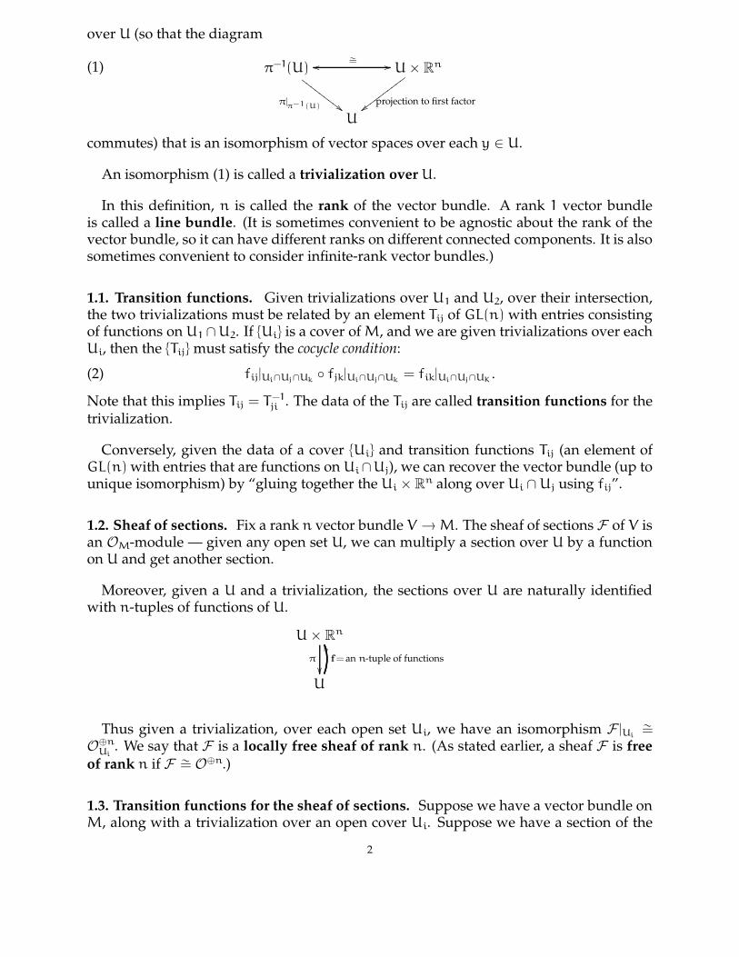
over U (so that the diagram

(1) π−1(U)

π|π−1(U) ##FF

FFFF

FFF

oo∼= // U × R

n

projection to first factor{{ww

wwww

wwww

U

commutes) that is an isomorphism of vector spaces over each y ∈ U.

An isomorphism (1) is called a trivialization over U.

In this definition, n is called the rank of the vector bundle. A rank 1 vector bundleis called a line bundle. (It is sometimes convenient to be agnostic about the rank of thevector bundle, so it can have different ranks on different connected components. It is alsosometimes convenient to consider infinite-rank vector bundles.)

1.1. Transition functions. Given trivializations over U1 and U2, over their intersection,the two trivializations must be related by an element Tij of GL(n) with entries consistingof functions on U1 ∩U2. If {Ui} is a cover of M, and we are given trivializations over eachUi, then the {Tij} must satisfy the cocycle condition:(2) fij|Ui∩Uj∩Uk

◦ fjk|Ui∩Uj∩Uk= fik|Ui∩Uj∩UK

.

Note that this implies Tij = T−1ji . The data of the Tij are called transition functions for the

trivialization.

Conversely, given the data of a cover {Ui} and transition functions Tij (an element ofGL(n) with entries that are functions on Ui ∩Uj), we can recover the vector bundle (up tounique isomorphism) by “gluing together the Ui × R

n along over Ui ∩ Uj using fij”.

1.2. Sheaf of sections. Fix a rank n vector bundle V → M. The sheaf of sections F of V isan OM-module — given any open set U, we can multiply a section over U by a functionon U and get another section.

Moreover, given a U and a trivialization, the sections over U are naturally identifiedwith n-tuples of functions of U.

U × Rn

π

��U

f= an n-tuple of functionsUU

Thus given a trivialization, over each open set Ui, we have an isomorphism F |Ui∼=

O⊕nUi

. We say that F is a locally free sheaf of rank n. (As stated earlier, a sheaf F is freeof rank n if F ∼= O⊕n.)

1.3. Transition functions for the sheaf of sections. Suppose we have a vector bundle onM, along with a trivialization over an open cover Ui. Suppose we have a section of the

2

vector bundle over M. (This discussion will apply with M replaced by any open subset.)Then over each Ui, the section corresponds to an n-tuple functions over Ui, say fi.

1.A. EXERCISE. Show that over Ui ∩ Uj, the vector-valued function fi is related to fj bythe transition functions:

Tijfi = fj

Given a locally free sheaf F with rank n, and a trivializing neighborhood of F (anopen cover {Ui} such that over each Ui, F |Ui

∼= O⊕nUi

as O-modules), we have transitionfunctions Tij ∈ GL(n,O(Ui ∩ Uj)) satisfying the cocycle condition (2). Thus in conclusionthe data of a locally free sheaf of rank n is equivalent to the data of a vector bundle ofrank n.

A rank 1 locally free sheaf is called an invertible sheaf. We’ll see later why it is calledinvertible; but it is still a somewhat heinous term for something so fundamental.

1.4. Locally free sheaves on schemes.

Suitably motivated, we now become rigorous and precise. We can generalize the notionof locally free sheaves to schemes without change. A locally free sheaf of rank n ona scheme X is an OX-module F that is locally trivial of rank n. Precisely, there is anopen cover {Ui} of X such that for each Ui, F |Ui

∼= O⊕nUi

. A locally free sheaf may bedescribed in terms of transition functions: the data of a cover {Ui} of X, and functionsTij ∈ GL(n,O(Ui ∩ Uj)) satisfying the cocycle condition (2). As before, given this data,we can find the sections over any open set U. Informally, they are sections of the freesheaves over each U ∩ Ui that agree on overlaps. More formally, for each i, they are

~si =

si1...

sin

∈ Γ(U ∩ Ui,OX)n, satisfying Tij~si = ~sj on U ∩ Ui ∩ Uj.

You should think of these “as” vector bundles, but just keep in mind that they arenot the “same”, just equivalent notions. We will later define the “total space” of thevector bundle V → X (a scheme over X) in terms of the sheaf version of Spec (precisely,Spec Sym V•). But the locally free sheaf perspective will prove to be more useful. As oneexample: the definition of a locally free sheaf is much shorter than that of a vector bundle.

As in our motivating discussion, it is sometimes convenient to let the rank vary amongconnected components, or to consider infinite rank locally free sheaves.

1.5. Useful constructions.

We now give some useful constructions in the form of a series of exercises. Most willlater generalize readily to quasicoherent sheaves.

1.B. EXERCISE. Suppose s is a section of a locally free sheaf F on a scheme X. Define thenotion of the subscheme cut out by s = 0. (Hint: given a trivialization over an open set

3

U, s corresponds to a number of functions f1, . . . on U; on U, take the scheme cut out bythese functions.)

1.C. EXERCISE. Suppose F and G are locally free sheaves on X of rank m and n respec-tively. Show that Hom(F ,G) is a locally free sheaf of rank mn.

1.D. EXERCISE. If E is a locally free sheaf of rank n, show that E∨ := Hom(E ,O) is also alocally free sheaf of rank n. This is called the dual of E . Given transition functions for E ,describe transition functions for E∨. (Note that if E is rank 1 (i.e. invertible), the transitionfunctions of the dual are the inverse of the transition functions of the original.) Showthat E ∼= E∨∨. (Caution: your argument showing that if there is a canonical isomorphism(F∨)∨ ∼= F better not also show that there is a canonical isomorphism F∨ ∼= F ! We’ll seean example soon of a locally free F that is not isomorphic to its dual. The example willbe the line bundle O(1) on P

1.)

1.E. EXERCISE. If F and G are locally free sheaves, show that F ⊗G is a locally free sheaf.(Here ⊗ is tensor product as OX-modules, defined last quarter) If F is an invertible sheaf,show that F ⊗ F∨ ∼= OX.

1.F. EXERCISE. Recall that tensor products tend to be only right-exact in general. Showthat tensoring by a locally free sheaf is exact. More precisely, if F is a locally free sheaf,and G ′

→ G → G ′′ is an exact sequence of OX-modules, then then so is G ′ ⊗F → G ⊗F →

G ′′ ⊗F .

1.G. EXERCISE. If E is a locally free sheaf, and F and G are OX-modules, show thatHom(F ,G ⊗ E) ∼= Hom(F ⊗ E∨,G).

1.H. EXERCISE AND IMPORTANT DEFINITION. Show that the invertible sheaves on X, upto isomorphism, form an abelian group under tensor product. This is called the Picardgroup of X, and is denoted Pic X. (For arithmetic people: this group, for the Spec of thering of integers R in a number field, is the class group of R.)

1.6. Random concluding remarks.

We define rational and regular sections of a locally free sheaf on a scheme X.

1.I. LESS IMPORTANT EXERCISE. Show that locally free sheaves on Noetherian normalschemes satisfy “Hartogs’ theorem”: sections defined away from a set of codimension atleast 2 extend over that set.

1.7. Remark. Based on your intuition for line bundles on manifolds, you might hope thatevery point has a “small” open neighborhood on which all invertible sheaves (or locallyfree sheaves) are trivial. Sadly, this is not the case. We will eventually see that for the

4

curve y2 − x3 − x = 0 in A2C

, every nonempty open set has nontrivial invertible sheaves.(This will use the fact that it is an open subset of an elliptic curve.)

1.J. EXERCISE (FOR ARITHMETICALLY-MINDED PEOPLE ONLY — I WON’T DEFINE MY TERMS).Prove that a fractional ideal on a ring of integers in a number field yields an invertiblesheaf. Show that any two that differ by a principal ideal yield the same invertible sheaf.Show that two that yield the same invertible sheaf differ by a principal ideal. The classgroup is defined to be the group of fractional ideals modulo the principal ideals. This ex-ercises shows that the class group is (isomorphic to) the Picard group. (This discussionapplies to the ring integers in any global field.)

1.8. The problem with locally free sheaves.

Recall that OX-modules form an abelian category: we can talk about kernels, cokernels,and so forth, and we can do homological algebra. Similarly, vector spaces form an abeliancategory. But locally free sheaves (i.e. vector bundles), along with reasonably naturalmaps between them (those that arise as maps of OX-modules), don’t form an abeliancategory. As a motivating example in the category of differentiable manifolds, considerthe map of the trivial line bundle on R (with co-ordinate t) to itself, corresponding tomultiplying by the co-ordinate t. Then this map jumps rank, and if you try to define akernel or cokernel you will get yourself confused.

This problem is resolved by enlarging our notion of nice OX-modules in a natural way,to quasicoherent sheaves.

OX-modules ⊃ quasicoherent sheaves ⊃ locally free sheavesabelian category abelian category not an abelian category

Similarly, finite rank locally free sheaves will sit in a nice smaller abelian category, thatof coherent sheaves.

quasicoherent sheaves ⊃ coherent sheaves ⊃ finite rank locally free sheavesabelian category abelian category not an abelian category

2. TOWARD QUASICOHERENT SHEAVES: THE DISTINGUISHED AFFINE BASE

Schemes generalize and geometrize the notion of “ring”. It is now time to define thecorresponding analogue of “module”, which is a quasicoherent sheaf.

One version of this notion is that of an OX-module. They form an abelian category, withtensor products.

We want a better one — a subcategory of OX-modules. Because these are the analoguesof modules, we’re going to define them in terms of affine open sets of the scheme. So let’sthink a bit harder about the structure of affine open sets on a general scheme X. I’m goingto define what I’ll call the distinguished affine base of the Zariski topology. This won’t be a

5

base in the sense that you’re used to. (For experts: it is a first example of a Grothendiecktopology.)

The open sets are the affine open subsets of X. We’ve already observed that this formsa base. But forget about that.

We like distinguished open sets Spec Af ↪→ Spec A, and we don’t really understandopen immersions of one random affine open subset in another. So we just remember the“nice” inclusions.

Definition. The distinguished affine base of a scheme X is the data of the affine opensets and the distinguished inclusions.

In other words, we are remembering only some of the open sets (the affine open sets),and only some of the morphisms between them (the distinguished morphisms). For ex-perts: if you think of a topology as a category (the category of open sets), we have de-scribed a subcategory.

We can define a sheaf on the distinguished affine base in the obvious way: we have aset (or abelian group, or ring) for each affine open set, and we know how to restrict todistinguished open sets.

Given a sheaf F on X, we get a sheaf on the distinguished affine base. You can guesswhere we’re going: we’ll show that all the information of the sheaf is contained in theinformation of the sheaf on the distinguished affine base.

As a warm-up, we can recover stalks as follows. (We will be implicitly using only thefollowing fact. We have a collection of open subsets, and some subsets, such that if wehave any x ∈ U, V where U and V are in our collection of open sets, there is some W

containing x, and contained in U and V such that W ↪→ U and W ↪→ V are both in ourcollection of inclusions. In the case we are considering here, this is the key fact that givenany two affine open sets Spec A, Spec B in X, Spec A ∩ Spec B could be covered by affineopen sets that were simultaneously distinguished in Spec A and Spec B. This is a cofinalcondition.)

The stalk Fx is the direct limit lim−→

(f ∈ F(U)) where the limit is over all open setscontained in U. We compare this to lim

−→(f ∈ F(U)) where the limit is over all affine open

sets, and all distinguished inclusions. You can check that the elements of one correspondto elements of the other. (Think carefully about this! It corresponds to the fact that thebasic elements are cofinal in this directed system.)

2.A. EXERCISE. Show that a section of a sheaf on the distinguished affine base is deter-mined by the section’s germs.

2.1. Theorem. —

6

(a) A sheaf on the distinguished affine base Fb determines a unique sheaf F , which whenrestricted to the affine base is Fb. (Hence if you start with a sheaf, and take the sheaf onthe distinguished affine base, and then take the induced sheaf, you get the sheaf you startedwith.)

(b) A morphism of sheaves on a distinguished affine base uniquely determines a morphism ofsheaves.

(c) An OX-module “on the distinguished affine base” yields an OX-module.

This proof is identical to our argument showing that sheaves are (essentially) the sameas sheaves on a base, using the “sheaf of compatible germs” construction. The mainreason for repeating it is to let you see that all that is needed is for the open sets to form acofinal system (or better, that the category of open sets and inclusions we are consideringis cofinal).

For experts: (a) and (b) are describing an equivalence of categories between sheaves onthe Zariski topology of X and sheaves on the distinguished affine base of X.

Proof. (a) Suppose Fb is a sheaf on the distinguished affine base. Then we can definestalks.

For any open set U of X, define the sheaf of compatible germsF(U) := {(fx ∈ Fb

x )x∈U : ∀x ∈ U, ∃Ux with x ⊂ Ux ⊂ U, Fx ∈ Fb(Ux) : Fxy = fy∀y ∈ Ux}

where each Ux is in our base, and Fxy means “the germ of Fx at y”. (As usual, those who

want to worry about the empty set are welcome to.)

This is a sheaf: convince yourself that we have restriction maps, identity, and gluability,really quite easily.

I next claim that if U is in our base, that F(U) = Fb(U). We clearly have a map Fb(U) →

F(U). This is an isomorphism on stalks, and hence an isomorphism by an Exercise fromlast quarter.

2.B. EXERCISE. Prove (b).

2.C. EXERCISE. Prove (c). �


7


RAVI VAKIL

CONTENTS

1. Quasicoherent sheaves 12. Quasicoherent sheaves form an abelian category 5

We began by recalling the distinguished affine base.

Definition. The distinguished affine base of a scheme X is the data of the affine opensets and the distinguished inclusions.

0.1. Theorem. —

(a) A sheaf on the distinguished affine base Fb determines a unique sheaf F , which whenrestricted to the affine base is Fb. (Hence if you start with a sheaf, and take the sheaf onthe distinguished affine base, and then take the induced sheaf, you get the sheaf you startedwith.)

(b) A morphism of sheaves on a distinguished affine base uniquely determines a morphism ofsheaves.

(c) An OX-module “on the distinguished affine base” yields an OX-module.

1. QUASICOHERENT SHEAVES

We now define the notion of quasicoherent sheaf. In the same way that a scheme is de-fined by “gluing together rings”, a quasicoherent sheaf over that scheme is obtained by“gluing together modules over those rings”. We will give two equivalent definitions; eachdefinition is useful in different circumstances. The first just involves the distinguishedtopology.

The first definition is more directly “sheafy”. Given an A-module M, we defined asheaf M on Spec A long ago — the sections over D(f) were Mf.

Definition A. An OX-module F is a quasicoherent sheaf if for every affine open Spec A,

F |Spec A∼= ˜Γ(Spec A,F).

Date: Wednesday, January 23, 2008.

1

(The “wide tilde” is supposed to cover the entire right side Γ(Spec A,F).) This isomor-phism is as sheaves of OX-modules.

Hence by this definition, the sheaves on Spec A correspond to A-modules. Given anA-module M, we get a sheaf M. Given a sheaf F on Spec A, we get an A-module Γ(X,F).These operations are inverse to each other. So in the same way as schemes are obtainedby gluing together rings, quasicoherent sheaves are obtained by gluing together modulesover those rings.

The second definition really focuses on the distinguished affine base, and is reminiscentof the Affine Covering Lemma.

Definition B. Suppose Spec Af ↪→ Spec A ⊂ X is a distinguished open set. Let φ :

Γ(Spec A,F) → Γ(Spec Af,F) be the restriction map. The source of φ is an A-module,and the target is an Af-module, so by the universal property of localization, φ naturallyfactors as:

Γ(Spec A,F)φ

//

((QQQQQQQQQQQQQΓ(Spec Af,F)

Γ(Spec A,F)f

α

66mmmmmmmmmmmmm

An OX-module F is a quasicoherent sheaf if for each such distinguished Spec Af ↪→

Spec A, α is an isomorphism.

Thus a quasicoherent sheaf is the data of one module for each affine open subset (amodule over the corresponding ring), such that the module over a distinguished open setSpec Af is given by localizing the module over Spec A. This will be an easy criterion tocheck.

1.1. Proposition. — Definitions A and B are the same.

Proof. Clearly Definition A implies Definition B. (Recall that the definition of M was interms of the distinguished topology on Spec A.) We now show that Definition B impliesDefinition A. By Definition B, the sections over any distinguished open Spec Af of M onSpec A is precisely Γ(Spec A,M)f, i.e. the sections of ˜Γ(Spec A,M) over Spec Af, and therestriction maps agree. Thus the two sheaves agree. �

We like Definition B because it says that to define a quasicoherent OX-module is thatwe just need to know what it is on all affine open sets, and that it behaves well underinverting a single element.

One reason we like Definition A is that it works well in gluing arguments, as in theproof of the following fact.

2

1.2. Proposition (quasicoherence is an affine-local notion). — Let X be a scheme, and F an OX-module. Then let P be the property of affine open sets that F |Spec A

∼= ˜Γ(Spec A,F). Then P is anaffine-local property.

Before we prove this, we give an exercise to show its utility.

1.A. EXERCISE. Show that locally free sheaves are quasicoherent.

Proof. By the Affine Communication Lemma, we must check two things. Clearly if Spec A

has property P, then so does the distinguished open Spec Af: if M is an A-module, thenM|Spec Af

∼= Mf as sheaves of OSpec Af-modules (both sides agree on the level of distin-

guished open sets and their restriction maps).

We next show the second hypothesis of the Affine Communication Lemma. Supposewe have modules M1, . . . , Mn, where Mi is an Afi

-module, along with isomorphisms φij :

(Mi)fj→ (Mj)fi

of Afifj-modules, satisfying the cocycle condition. We want to construct

an M such that M gives us Mi on D(fi) = Spec Afi, or equivalently, isomorphisms ρi :

Γ(D(fi), M) → Mi, so that the bottom triangle of(1) M

⊗Afi

zzuuuu

uuuu

uu ⊗Afj

$$IIII

IIII

II

Mfi

ρi

∼

||xxxx

xxxx

x ⊗Afj

$$HHHHHH

HHH

Mfj

ρj

∼

""FFFFFFFF⊗Afj

zzvvvv

vvvv

v

Mi

⊗Afi ""FFFF

FFFF

FMfifj;;

∼

{{vvvv

vvvv

v cc

∼

##HHHH

HHHHH

Mj

⊗Afj||xxxx

xxxx

x

(Mi)fj

φij

∼

// (Mj)fi

commutes.

We already know that M should be the sections of F over Spec A, as F is a sheaf.Consider elements of M1 × · · · × Mn that “agree on overlaps”; let this set be M. Then

0 → M → M1 × · · · × Mn → M12 × M13 × · · · × M(n−1)n

is an exact sequence (where Mij = (Mi)fj∼= (Mj)fi

, and the latter morphism is the “dif-ference” morphism). So M is a kernel of a morphism of A-modules, hence an A-module.We are left to show that Mi

∼= Mfi(and that this isomorphism satisfies (1)).

For convenience we assume i = 1. Localization is exact, so(2)0 // Mf1

// M1 × (M2)f1× · · · × (Mn)f1

// M12 × · · · × (M23)f1× · · · × (M(n−1)n)f1

is an exact sequence of Af1-modules.

We now identify many of the modules appearing in (2) in terms of M1. First of all, f1

is invertible in Af1, so (M1)f1

is canonically M1. Also, (Mj)f1∼= (M1)fj

via φij. Hence if

3

i, j 6= 1, (Mij)f1∼= (M1)fifj

via φ1i and φ1j (here the cocycle condition is implicitly used).Furthermore, (M1i)f1

∼= (M1)fivia φ1i. Thus we can write (2) as

(3)0 // Mf1

// M1 × (M1)f2× · · · × (M1)fn

α // (M1)f2× · · · × (M1)fn

× (M1)f2f3× · · · (M1)fn−1fn

By assumption, F |Spec Af1is quasicoherent, so by considering the cover of

Spec Af1= Spec Af1

∪ Spec Af1f2∪ Spec Af1f3

∪ · · · ∪ Spec Af1fn

(which indeed has a “redundant” first term), and identifying sections of F over Spec Af1

in terms of sections over the open sets in the cover and their pairwise overlaps, we havean exact sequence of Af1

-modules

0 // M1// M1 × (M1)f2

× · · · × (M1)fn

β// (M1)f2

× · · · × (M1)fn× (M1)f2f3

× · · · (M1)fn−1fn

which is very similar to (3). Indeed, the final map β of the above sequence is the same asthe map α of (3), so ker α = ker β, i.e. we have an isomorphism M1

∼= Mf1.

Finally, the triangle of (1) is commutative, as each vertex of the triangle can be identifiedas the sections of F over Spec Af1f2

. �

1.B. IMPORTANT EXERCISE. Suppose X is a quasicompact and quasiseparated scheme(i.e. covered by a finite number of affine open sets, the pairwise intersection of whichis also covered by a finite number of affine open sets). Suppose F is a quasicoherentsheaf on X, and let f ∈ Γ(X,OX) be a function on X. Show that the restriction mapresXf⊂X : Γ(X,F) → Γ(Xf,F) (here Xf is the open subset of X where f doesn’t vanish) is pre-cisely localization. In other words show that there is an isomorphism Γ(X,F)f → Γ(Xf,F)

making the following diagram commute.

Γ(X,F)resXf⊂X

//

⊗AAf %%LLLLLLLLLLΓ(Xf,F)

Γ(X,F)f

∼

88rrrrrrrrrr

All that you should need in your argument is that X admits a cover by a finite numberof open sets, and that their pairwise intersections are each quasicompact. (Hint: cover byaffine open sets. Use the sheaf property. A nice way to formalize this is the following.Apply the exact functor ⊗AAf to the exact sequence

0 → Γ(X,F) → ⊕iΓ(Ui,F) → ⊕Γ(Uijk,F)

where the Ui form a finite cover of X and Uijk form an affine cover of Ui ∩ Uj.)

1.C. LESS IMPORTANT EXERCISE. Give a counterexample to show that the above state-ment need not hold if X is not quasicompact. (Possible hint: take an infinite disjoint unionof affine schemes. The key idea is that infinite direct sums do not commute with localiza-tion.)

4

1.D. IMPORTANT EXERCISE (COROLLARY TO EXERCISE 1.B). Suppose π : X → Y is aquasicompact quasiseparated morphism, and F is a quasicoherent sheaf on X. Show thatπ∗F is a quasicoherent sheaf on Y.

1.E. UNIMPORTANT EXERCISE (NOT EVERY OX-MODULE IS A QUASICOHERENT SHEAF).(a) Suppose X = Spec k[t]. Let F be the skyscraper sheaf supported at the origin [(t)],with group k(t) and the usual k[t]-module structure. Show that this is an OX-module thats not a quasicoherent sheaf. (More generally, if X is an integral scheme, and p ∈ X thatis not the generic point, we could take the skyscraper sheaf at p with group the functionfield of X. Except in a silly circumstances, this sheaf won’t be quasicoherent.)(b) Suppose X = Spec k[t]. Let F be the skyscraper sheaf supported at the generic point[(0)], with group k(t). Give this the structure of an OX-module. Show that this is a quasi-coherent sheaf. Describe the restriction maps in the distinguished topology of X.

2. QUASICOHERENT SHEAVES FORM AN ABELIAN CATEGORY

The category of A-modules is an abelian category. Indeed, this is our motivating ex-ample of our notion of abelian category. Similarly, quasicoherent sheaves form an abeliancategory. I’ll explain how.

When you show that something is an abelian category, you have to check many things,because the definition has many parts. However, if the objects you are considering lie insome ambient abelian category, then it is much easier. As a metaphor, there are severalthings you have to do to check that something is a group. But if you have a subset ofgroup elements, it is much easier to check that it forms a subgroup.

You can look at back at the definition of an abelian category, and you’ll see that inorder to check that a subcategory is an abelian subcategory, you need to check only thefollowing things:

(i) 0 is in your subcategory(ii) your subcategory is closed under finite sums

(iii) your subcategory is closed under kernels and cokernels

In our case of{quasicoherent sheaves} ⊂ {OX-modules},

the first two are cheap: 0 is certainly quasicoherent, and the subcategory is closed underfinite sums: if F and G are sheaves on X, and over Spec A, F ∼= M and G ∼= N, thenF ⊕ G = M ⊕ N, so F ⊕ G is a quasicoherent sheaf.

We now check (iii). Suppose α : F → G is a morphism of quasicoherent sheaves.Then on any affine open set U, where the morphism is given by β : M → N, define(ker α)(U) = ker β and (coker α)(U) = coker β. Then these behave well under inversion ofa single element: if

0 → K → M → N → P → 0

5

is exact, then so is0 → Kf → Mf → Nf → Pf → 0,

from which (ker β)f∼= ker(βf) and (coker β)f

∼= coker(βf). Thus both of these definequasicoherent sheaves. Moreover, by checking stalks, they are indeed the kernel andcokernel of α (exactness can be checked stalk-locally ). Thus the quasicoherent sheavesindeed form an abelian category.

2.A. EXERCISE. Show that a sequence of quasicoherent sheaves F → G → H on X isexact if and only if it is exact on each open set in an affine cover of X. (In particular,taking sections over an affine open Spec A is an exact functor from the category of qua-sicoherent sheaves on X to the category of A-modules. Recall that taking sections is onlyleft-exact in general.) In particular, we may check injectivity or surjectivity of a morphismof quasicoherent sheaves by checking on an affine cover.

Warning: If 0 → F → G → H → 0 is an exact sequence of quasicoherent sheaves, thenfor any open set

0 → F(U) → G(U) → H(U)

is exact, and we have exactness on the right is guaranteed to hold only if U is affine. (Toset you up for cohomology: whenever you see left-exactness, you expect to eventuallyinterpret this as a start of a long exact sequence. So we are expecting H1’s on the right,and now we expect that H1(Spec A,F) = 0. This will indeed be the case.)

2.B. EXERCISE (CONNECTION TO ANOTHER DEFINITION). Show that an OX-module Fon a scheme X is quasicoherent if and only if there exists an open cover by Ui such thaton each Ui, F |Ui

is isomorphic to the cokernel of a map of two free sheaves:O⊕I

Ui→ O⊕J

Ui→ F |Ui

→ 0

is exact. We have thus connected our definitions to the definition given at the very startof the chapter.

We then began to discuss module-like constructions for quasicoherent sheaves, and I’veleft these for the next day’s notes, so all of our discussion on that topic is in one place.


6


RAVI VAKIL

CONTENTS

1. Module-like constructions 12. Finiteness conditions on quasicoherent sheaves: finite type quasicoherent

sheaves, and coherent sheaves 33. Coherent modules over non-Noetherian rings ?? 64. Pleasant properties of finite type and coherent sheaves 8

1. MODULE-LIKE CONSTRUCTIONS

In a similar way, basically any nice construction involving modules extends to quasico-herent sheaves.

As an important example, we consider tensor products.

1.A. EXERCISE. If F and G are quasicoherent sheaves, show that F ⊗ G is a quasi-coherent sheaf described by the following information: If Spec A is an affine open, andΓ(Spec A,F) = M and Γ(Spec A,G) = N, then Γ(Spec A,F ⊗ G) = M ⊗ N, and the restric-tion map Γ(Spec A,F⊗G) → Γ(Spec Af,F⊗G) is precisely the localization map M⊗AN →(M⊗A N)f

∼= Mf⊗AfNf. (We are using the algebraic fact that (M⊗R N)f

∼= Mf⊗RfNf. You

can prove this by universal property if you want, or by using the explicit construction.)

Note that thanks to the machinery behind the distinguished affine base, sheafificationis taken care of. This is a feature we will use often: constructions involving quasicoherentsheaves that involve sheafification for general sheaves don’t require sheafification whenconsidered on the distinguished affine base. Along with the fact that injectivity, surjec-tivity, kernels and so on may be computed on affine opens, this is the reason that it isparticularly convenient to think about quasicoherent sheaves in terms of affine open sets.

1.B. EASY EXERCISE. Show that the stalk of the tensor product of quasicoherent sheavesat a point is the tensor product of the stalks.


1

Given a section s of F and a section t of G, we have a section s ⊗ t of F ⊗ G. If eitherF or G is an invertible sheaf, this section is denoted st.

1.1. Tensor algebra constructions.

For the next exercises, recall the following. If M is an A-module, then the tensor algebraT ∗(M) is a non-commutative algebra, graded by Z≥0, defined as follows. T 0(M) = A,Tn(M) = M ⊗A · · · ⊗A M (where n terms appear in the product), and multiplication iswhat you expect. The symmetric algebra Sym∗ M is a symmetric algebra, graded by Z≥0,defined as the quotient of T ∗(M) by the (two-sided) ideal generated by all elements ofthe form x ⊗ y − y ⊗ x for all x, y ∈ M. Thus Symn M is the quotient of M ⊗ · · · ⊗ M

by the relations of the form m1 ⊗ · · · ⊗ mn − m ′1 ⊗ · · · ⊗ m ′

n where (m ′1, . . . , m

′n) is a

rearrangement of (m1, . . . , mn). The exterior algebra ∧∗M is defined to be the quotient ofT ∗M by the (two-sided) ideal generated by all elements of the form x ⊗ y + y ⊗ x forall x, y ∈ M. Thus ∧nM is the quotient of M ⊗ · · · ⊗ M by the relations of the formm1 ⊗ · · · ⊗ mn − (−1)sgn(σ)mσ(1) ⊗ · · · ⊗ mσ(n) where σ is a permutation of {1, . . . , n}. Itis a “skew-commutative” A-algebra. It is most correct to write T ∗

A(M), Sym∗A(M), and

∧∗A(M), but the “base ring” A is usually omitted for convenience. (Better: both Sym

and ∧ are defined by universal properties. For example, SymnA(M) is universal among

modules such that any map of A-modules M⊗n → N that is symmetric in the n entriesfactors uniquely through Symn

A(M).)

1.C. EXERCISE. Suppose F is a quasicoherent sheaf. Define the quasicoherent sheavesSymn F and ∧nF . (One possibility: describe them on each affine open set.) If F is locallyfree of rank m, show that TnF , Symn F , and ∧nF are locally free, and find their ranks.

You can also define the sheaf of non-commutative algebras T ∗F , the sheaf of commuta-tive algebras Sym∗ F , and the sheaf of skew-commutative algebras ∧∗F .

1.D. EXERCISE (POSSIBLE HELP FOR LATER PROBLEMS). Suppose 0 → F ′ → F → F ′′ → 0

is a short exact sequence of locally free sheaves on X. Suppose U = Spec A is an affineopen set where F ′, F ′′ are free, say F ′|Spec A = Aa, F ′′|Spec A = Ab. Show that F is alsofree, and that 0 → F ′ → F → F ′′ → 0 can be interpreted as coming from the tautologicalexact sequence 0 → Aa → Aa+b → Ab → 0. Show that given such an open cover, thetransition matrices of F may be interpreted as block upper-diagonal matrices, where thettop a × a block are transition matrices for F ′, and the bottom b × b blocks are transitionmatrices for F ′′.

1.E. IMPORTANT EXERCISE. Suppose 0 → F ′ → F → F ′′ → 0 is an exact sequence oflocally free sheaves. Show that for any r, there is a filtration of Symr F

Symr F = F0 ⊇ F1 ⊇ · · · ⊇ Fr ⊃ Fr+1 = 0

with subquotients

Fp/Fp+1 ∼= (Symp F ′) ⊗ (Symr−p F ′′).

2

(Possible hint for this, and Exercise 1.G: It suffices to consider a small enough affine openset Spec A, where F ′, F , F ′′ are free, and to show that your construction behaves wellwith respect to localization at an element f ∈ A. In such an open set, the sequence is0 → Ap → Ap+q → Aq → 0 by the Exercise 1.D. Let e1, . . . , en be the standard basis of An,and f1, . . . , fq be the the standard basis of Aq. Let e ′

1, . . . , e ′p be denote the images of e1,

. . . , ep in Ap+q. Let f ′1, . . . , f ′

q be any lifts of f1, . . . , fq to Ap+q. Note that f ′i is well-defined

modulo e ′1, . . . , e ′

p. Note that

Syms F |Spec A∼= ⊕s

i=0 Symi F ′|Spec A ⊗OSpec ASyms−i F ′′|Spec A.

Show that Fp := ⊕si=p Symi F ′|Spec A ⊗OSpec A

Syms−i F ′′|Spec A gives a well-defined (locallyfree) subsheaf that is independent of the choices made, e.g. of the basis e1, . . . , ep (this isin GLp(A)), f1, . . . , fq (this is in GLq(A)), and the lifts f ′

1, . . . , f ′q.)

1.F. EXERCISE. Suppose F is locally free of rank n. Then ∧nF is called the deter-minant (line) bundle or (perhaps better) determinant locally free sheaf. Show that∧rF × ∧n−rF → ∧nF is a perfect pairing for all r.

1.G. EXERCISE. Suppose 0 → F ′ → F → F ′′ → 0 is an exact sequence of locally freesheaves. Show that for any r, there is a filtration of ∧rF :

∧rF = F0 ⊇ F1 ⊇ · · · ⊇ Fr ⊃ Fr+1 = 0

with subquotientsFp/Fp+1 ∼= (∧pF ′) ⊗ (∧r−pF ′′)

for each p. In particular, detF = (detF ′) ⊗ (detF ′′). In fact we only need that F ′′ islocally free.

1.H. EXERCISE (DETERMINANT LINE BUNDLES BEHAVE WELL IN EXACT SEQUENCES).Suppose 0 → F1 → · · · → Fn → 0 is an exact sequence of finite rank locally free sheaveson X. Show that “the alternating product of determinant bundles is trivial”:

det(F1) ⊗ det(F2)∨ ⊗ det(F3) ⊗ det(F4)

∨ ⊗ · · · ∼= OX.

1.2. Torsion-free sheaves (a stalk-local condition). Recall that an A-module M is torsion-free if rm = 0 implies r = 0 or m = 0. An OX-module F is said to be torsion-free if Fp isa torsion-free OX,p-module for all p.

1.I. EXERCISE. Show that if M is a torsion-free A-module, then so is any localization ofM. Hence show that M is a torsion free sheaf on Spec A.

1.J. UNIMPORTANT EXERCISE (TORSION-FREENESS IS NOT AFFINE LOCAL FOR STUPIDREASONS). Find an example on a two-point space showing that M := A might notbe torsion-free on Spec A even though OSpec A = M is torsion-free.

3

2. FINITENESS CONDITIONS ON QUASICOHERENT SHEAVES: FINITE TYPEQUASICOHERENT SHEAVES, AND COHERENT SHEAVES

There are some natural finiteness conditions on an A-module M. I will tell you three.In the case when A is a Noetherian ring, which is the case that almost all of you will evercare about, they are all the same.

The first is the most naive: a module could be finitely generated. In other words, thereis a surjection Ap → M → 0.

The second is reasonable too. It could be finitely presented — it could have a finitenumber of generators with a finite number of relations: there exists a finite presentation

Aq → Ap → M → 0.

The third notion is frankly a bit surprising, and I’ll justify it soon. We say that an A-module M is coherent if (i) it is finitely generated, and (ii) whenenver we have a mapAp → M (not necessarily surjective!), the kernel is finitely generated.

Clearly coherent implies finitely presented, which in turn implies finitely generated.

2.1. Proposition. — If A is Noetherian, then these three definitions are the same.

Before proving this, we take this as an excuse to develop some algebraic background.

2.2. Noetherian conditions for modules. If A is any ring, not necessarily Noetherian, we sayan A-module is Noetherian if it satisfies the ascending chain condition for submodules.Thus for example A is a Noetherian ring if and only if it is a Noetherian A-module.

2.A. EXERCISE. Show that if M is a Noetherian A-module, then any submodule of M isa finitely generated A-module.

2.B. EXERCISE. If 0 → M ′ → M → M ′′ → 0 is exact, show that M ′ and M ′′ areNoetherian if and only if M is Noetherian. (Hint: Given an ascending chain in M, weget two simultaneous ascending chains in M ′ and M ′′. Possible further hint: prove that if

M ′ // Mφ

// M ′′ is exact, and N, N ′ ⊂ M, and N∩M ′ = N ′∩M ′ and φ(N) = φ(N ′),then N = N ′.)

2.C. EXERCISE. Show that if A is a Noetherian ring, then An is a Noetherian A-module.

2.D. EXERCISE. Show that if A is a Noetherian ring and M is a finitely generated A-module, then M is a Noetherian module. Hence by Exercise 2.A, any submodule of afinitely generated module over a Noetherian ring is finitely generated.

4

Proof of Proposition 2.1. As we observed earlier, coherent implies finitely presented im-plies finitely generated. So suppose M is finitely generated. Take any Ap α

// M . Thenker α is a submodule of a finitely generated module over A, and is thus finitely generatedby Exercise 2.D. Thus M is coherent. �

Hence most normal people can think of these three notions as the same thing.

2.3. Proposition. — The coherent A-modules form an abelian subcategory of the category ofA-modules.

The proof in general is given in §3 in a series of short exercises.

Proof if A is Noetherian. Recall from our discussion a few classes ago that we must checkthree things:

(i) The 0-sheaf is coherent.(ii) The category of coherent modules is closed under finite sums.

(iii) The category of coherent modules is closed under kernels and cokernels

The first two are clear. For (iii), suppose that f : M → N is a map of finitely generatedmodules. Then coker f is finitely generated (it is the image of N), and ker f is too (it is asubmodule of a finitely generated module over a Noetherian ring, Exercise 2.D). �

2.E. EASY EXERCISE (ONLY IMPORTANT FOR NON-NOETHERIAN PEOPLE). Show A iscoherent as an A-module if and only if the notion of finitely presented agrees with thenotion of coherent.

2.F. EXERCISE. If f ∈ A, show that if M is a finitely generated (resp. finitely presented,coherent) A-module, then Mf is a finitely generated (resp. finitely presented, coherent)Af-module. (The “coherent” case is the tricky one.)

2.G. EXERCISE. If (f1, . . . , fn) = A, and Mfiis finitely generated (resp. coherent) Afi

-module for all i, then M is a finitely generated (resp. coherent) A-module.

Definition. A quasicoherent sheaf F is finite type (resp. coherent) if for every affineopen Spec A, Γ(Spec A,F) is a finitely generated (resp. coherent) A-module.

Thanks to the affine communication lemma, and the two previous exercises 2.F and 2.G,it suffices to check this on the open sets in a single affine cover.

I want to say a few words on the notion of coherence. I see Proposition 2.3 as a goodmotivation for this definition: it gives a small (in a non-technical sense) abelian categoryin which we can think about vector bundles.

5

There are two sorts of people who should care about the details of this definition (asopposed to working in a Noetherian world and always thinking that coherent equalsfinite type). Complex geometers should care. They consider complex-analytic spaceswith the classical topology. One can define the notion of coherent OX-module in a wayanalogous to this. Then Oka’s theorem states that the structure sheaf is coherent, andthis is very hard.

The second sort of people who should care are the sort of arithmetic people who some-times are forced to consider non-Noetherian rings. For example, the ring of adeles is non-Noetherian.

Warning: it is common in the later literature to incorrectly define coherent as finitelygenerated. Please only use the correct definition, as the wrong definition only causesconfusion. I will try to be scrupulous about this. Besides doing this for the reason ofhonesty, it will also help you see what hypotheses are actually necessary to prove things.And that always helps you remember what the proofs are — and hence why things aretrue.

3. COHERENT MODULES OVER NON-NOETHERIAN RINGS ??

This section is intended for people who might work with non-Noetherian rings, or whootherwise might want to understand coherent sheaves in a more general setting. Read thisonly if you really want to!

Suppose A is a ring. Recall that an A-module M is finitely generated if there is a surjectionAn → M → 0. It is finitely presented if there is a presentation Am → An → M → 0. AndM is coherent if (i) M is finitely generated, and (ii) every map An → M has a finitelygenerated kernel. The reason we like this third definition is that coherent modules forman abelian category.

Here are some quite accessible exercises working out why these notions behave well.Some repeat earlier discussion in order to keep this section self-contained.

3.A. EXERCISE. Show that coherent implies finitely presented implies finitely generated.(This was discussed in the previous section.)

3.B. EXERCISE. Show that 0 is coherent.

Suppose for problems 3.C–3.I that

(1) 0 → M → N → P → 0

is an exact sequence of A-modules. In thise series of problems, we will show that if twoof (1) are coherent, the third is as well, whiich will prove very useful.

6

Hint ?. Here is a hint which applies to several of the problems: try to write

0 // Ap //

��

Ap+q //

��

Aq //

��

0

0 // M // N // P // 0

and possibly use the Snake Lemma.

3.C. EXERCISE. Show that N finitely generated implies P finitely generated. (You willonly need right-exactness of (1).)

3.D. EXERCISE. Show that M, P finitely generated implies N finitely generated. (Possiblehint: ?.) (You will only need right-exactness of (1).)

3.E. EXERCISE. Show that N, P finitely generated need not imply M finitely generated.(Hint: if I is an ideal, we have 0 → I → A → A/I → 0.)

3.F. EXERCISE. Show that N coherent, M finitely generated implies M coherent. (Youwill only need left-exactness of (1).)

3.G. EXERCISE. Show that N, P coherent implies M coherent. Hint for (i):

Aq

��

!!DD

D

D

D

D

D

D

Ap

�� AA

A

A

A

A

A

A

0 // M

��

// N

��

// P //

��>

>

>

>

>

>

>

0

0 0 0

(You will only need left-exactness of (1).)

3.H. EXERCISE. Show that M finitely generated and N coherent implies P coherent. (Hintfor (ii): ?.)

3.I. EXERCISE. Show that M, P coherent implies N coherent. (Hint: ?.)

3.J. EXERCISE. Show that a finite direct sum of coherent modules is coherent.

3.K. EXERCISE. Suppose M is finitely generated, N coherent. Then if φ : M → N is anymap, then show that Im φ is coherent.

7

3.L. EXERCISE. Show that the kernel and cokernel of maps of coherent modules arecoherent.

At this point, we have verified that coherent A-modules form an abelian subcategoryof the category of A-modules. (Things you have to check: 0 should be in this set; it shouldbe closed under finite sums; and it should be closed under taking kernels and cokernels.)

3.M. EXERCISE. Suppose M and N are coherent submodules of the coherent module P.Show that M + N and M ∩ N are coherent. (Hint: consider the right map M ⊕ N → P.)

3.N. EXERCISE. Show that if A is coherent (as an A-module) then finitely presentedmodules are coherent. (Of course, if finitely presented modules are coherent, then A iscoherent, as A is finitely presented!)

3.O. EXERCISE. If M is finitely presented and N is coherent, show that Hom(M, N) iscoherent. (Hint: Hom is left-exact in its first entry.)

3.P. EXERCISE. If M is finitely presented, and N is coherent, show that M⊗N is coherent.

3.Q. EXERCISE. If f ∈ A, show that if M is a finitely generated (resp. finitely presented,coherent) A-module, then Mf is a finitely generated (resp. finitely presented, coherent)Af-module. (Hint: localization is exact.) (This exercise appeared earlier as Exercise 2.F.)

3.R. EXERCISE. Suppose (f1, . . . , fn) = A. Show that if Mfiis finitely generated for all i,

then M is too. (Hint: Say Mfiis generated by mij ∈ M as an Afi

-module. Show that themij generate M. To check surjectivity ⊕i,jA → M, it suffices to check “on D(fi)” for all i.)

3.S. EXERCISE. Suppose (f1, . . . , fn) = A. Show that if Mfiis coherent for all i, then M is

too. (Hint: if φ : A2 → M, then (ker φ)fi= ker(φfi

), which is finitely generated for all i.Then apply the previous exercise.)

3.T. EXERCISE. Show that the ring A := k[x1, x2, . . . ] is not coherent over itself. (Hint:consider A → A with x1, x2, . . . 7→ 0.) Thus we have an example of a finitely presentedmodule that is not coherent; a surjection of finitely presented modules whose kernel isnot even finitely generated; hence an example showing that finitely presented modulesdon’t form an abelian category.

4. PLEASANT PROPERTIES OF FINITE TYPE AND COHERENT SHEAVES

4.A. EXERCISE. Suppose F is a coherent sheaf on X, and G is a quasicoherent sheaf onX. Show that Hom(F ,G). (Hint: Describe it on affine open sets, and show that it be-haves well with respect to localization with respect to f. To show that HomA(M, N)f

∼=

8

HomAf(Mf, Nf), take a presentation Aq → Ap → M → 0, and apply Hom(·, N) and lo-

calize. You will use the fact that p and q are finite.) If further G is coherent, show thatHom(F ,G) is also coherent. Show that Hom is a left-exact functor in both variables.

Recall that Hom(F ,OX) is called the dual of F , and is denoted F∨.

4.B. USEFUL EXERCISE: GEOMETRIC NAKAYAMA. Suppose X is a scheme, and F is afinite type quasicoherent sheaf. Show that if x ∈ U ⊂ X is a neighborhood of x in X

and a1, . . . , an ∈ F(U) so that the images a1, . . . , an ∈ Fx generate F ⊗ k(x), then thereis a neighborhood x ⊂ V ⊂ U of x so that a1|V , . . . , an|V generate F |V . In particular, ifFx ⊗ k(x) = 0, then there exists V such that F |V = 0.

4.C. LESS IMPORTANT EXERCISE. Suppose F and G are finite type sheaves such thatF ⊗ G ∼= OX. Then F and G are both invertible (Hint: Nakayama.) This is the reasonfor the adjective “invertible”: these sheaves are the invertible elements of the “monoid offinite type sheaves”.

4.1. The support of a finite type sheaf is closed. Recall the definition of support of asection of a sheaf, and of a sheaf.

Suppose F is a sheaf of abelian groups (resp. OX-module) on a topological space X

(resp. ringed space (X,OX)). Define the support of a section s of F to be

Supp s = {p ∈ X : sp 6= 0 in Fp}.

I think of this as saying where s “lives”. Define the support of F as

SuppF = {p ∈ X : Fp 6= 0}.

It is the union of “all the supports of sections on various open sets”. I think of this assaying where F “lives”. Caution. This is where the germ(s) are nonzero, not where thevalue(s) are nonzero.

Support is a stalk-local notion, and hence behaves well with respect to restriction toopen sets, or to stalks.

4.D. EXERCISE. The support of a finite type quasicoherent sheaf on a scheme X is aclosed subset. (Hint: Reduce to the case X affine. Choose a finite set of generators of thecorresponding module.) Show that the support of a quasicoherent sheaf need not beclosed. (Hint: If A = C[t], then C[t]/(t − a) is an A-module supported at a. Consider⊕a∈CC[t]/(t−a). Warning: this example won’t work if ⊕ is replaced by

∏, so be careful!)

4.2. Rank of a finite type sheaf at a point.

The rank F of a finite type sheaf at a point p is dimk Fp/mFp where m is the maximalideal corresponding to p. More explicitly, on any affine set Spec A where p = [p] andF(Spec A) = M, then the rank is dimFF(A/p) Mp/pMp. The rank is finite because of the

9

finite type hypothesis. By Nakayama’s lemma (again using the finite type condition), thisis the minimal number of generators of Mp as an Ap-module.

If F is quasicoherent (not necessarily finite type), then Fp/mFp can be interpreted asthe fiber of the sheaf at the point. A section of F over an open set containing p can be saidto take on a value at that point, which is an element of Fp/mFp.

4.E. EXERCISE. Show that at any point, rank(F ⊕ G) = rank(F) + rank(G) and rank(F ⊗

G) = rankF rankG at any point. (Hint: Show that direct sums and tensor products com-mute with ring quotients and localizations, i.e. (M ⊕ N) ⊗R (R/I) ∼= M/IM ⊕ N/IN,(M ⊗R N) ⊗R (R/I) ∼= (M ⊗R R/I) ⊗R/I (N ⊗R R/I) ∼= M/IM ⊗R/I N/IM, etc.)

4.F. EXERCISE. Show that rank(F) is an upper semicontinuous function on X. (Hint:Generators at P are generators nearby.)

Note that this definition of rank is consistent with the notion of rank of a locally freesheaf. In the locally free case, the rank is a (locally) constant function of the point. Theconverse is sometimes true, as is shown in Exercise 4.G below.

4.G. IMPORTANT HARD EXERCISE. (a) If X is reduced, F is coherent, and the rank isconstant, show that F is locally free. (Hint: choose a point p ∈ X, and choose generatorsof the stalk Fp. Let U be an open set where the generators are sections, so we have amap φ : O⊕n

U → F |U. The cokernel and kernel of φ are supported on closed sets by Exer-cise 4.D. Show that these closed subsets don’t include p. Make sure you use the reducedhypothesis!) Thus (as rank is uppersemicontinuous, Exercise 4.F) coherent sheaves arelocally free on a dense open set. Hint: Reduce to the case where X is affine, say Spec A, sothe closed points are dense. Then show it in a neighborhood of a closed point [m]. Choosem1, . . . , mn generators of M/mM, and lift them to elements of M. Then they generate M,by Nakayama’s Lemma. Let φ : An → M with (r1, . . . , rn) 7→

∑rimi. Let K be the

cokernel, which is finitely generated. Then Km = 0 (because ⊗Am is right-exact), so thereis an f ∈ A such that Kf = 0 (take the product of the annihilators of a finite generating setof K). Replace A by Af. We now have that coker φ = 0, and we want to prove ker φ = 0.Otherwise, say (r1, . . . , rn) is in the kernel, with r1 6= 0. As r1 6= 0, there is some p wherer1 /∈ p — here we use the reduced hypothesis. Then r1 is invertible in Ap, so Mp has fewerthan n generators, contradicting the constancy of rank.(b) Show that part (a) can be false without the condition of X being reduced. (Hint:Spec k[x]/x2, M = k.)

You can use the notion of rank to help visualize finite type sheaves, or even quasico-herent sheaves. I drew some pictures in class, but I haven’t figured out yet how to latexthem up.


10


RAVI VAKIL

CONTENTS

1. Quasicoherent sheaves of ideals, and closed subschemes 12. Invertible sheaves (line bundles) and divisors 23. Some line bundles on projective space 24. Effective Cartier divisors “=” invertible ideal sheaves 4

1. QUASICOHERENT SHEAVES OF IDEALS, AND CLOSED SUBSCHEMES

The point of this section is that closed subschemes correspond precisely to quasicoher-ent sheaves of ideals.

Recall that if i : X ↪→ Y is a closed immersion, then we have a surjection of sheaves onY: OY

// // i∗OX . (The i∗ is often omitted, as we are considering the sheaf on X as beinga sheaf on Y.) The sheaf i∗OX is quasicoherent on Y; this is in some sense the definition of“closed subscheme”. The kernel IX/Y is a “sheaf of ideals” in Y: for each open subset ofY, the sections form an ideal in the ring of functions of Y. As quasicoherent sheaves on Y

form an abelian category, IX/Y is a quasicoherent sheaf of ideals.

Conversely, a quasicoherent sheaf of ideals I ↪→ OY defines a closed subscheme. Thiswas stated in slightly different language in Exercise 1. Precisely, I is quasicoherent pre-cisely if, for each distinguished open Spec Af ↪→ Spec A, I(Spec Af) = I(Spec A)f (Defini-tion B of quasicoherent sheaves), and this was one criterion for when ideals in affine opensets define a closed subscheme (Exercise 1). (An example of a non-quasicoherent sheaf ofideals was given in an earlier Exercise.)

We call

(1) 0 → IX/Y → OY → i∗OX → 0

the closed subscheme exact sequence corresponding to X ↪→ Y.

Date: Monday, January 28, 2008. Mild correction Feb. 19 (thanks Nathan!).

1

2. INVERTIBLE SHEAVES (LINE BUNDLES) AND DIVISORS

We next develop some mechanism of understanding invertible sheaves (line bundles)on a given scheme X. Recall that Pic X is the group of invertible sheaves on X. Ourgoal will be to develop convenient and powerful ways of describing and working withinvertible sheaves.

We begin by describing invertible sheaves on projective space (over a field). We thendiscuss sheaves of ideals that happen to be invertible (effective Cartier divisors). Partiallymotivated by this insight that invertible sheaves correspond to “codimension 1 informa-tion”, we will discuss the theory of Weil divisors, and use this to actually compute Pic X

in a number of circumstances.

3. SOME LINE BUNDLES ON PROJECTIVE SPACE

We now describe a family of invertible sheaves on projective space over a field k.

As a warm-up, we begin with the invertible sheaf OP1k(1) on P

1k = Proj k[x0, x1]. (The

subscript P1k refers to the space on which the sheaf lives, and is often omitted when it is

clear from the context.) We describe the invertible sheaf O(1) using transition functions.It is trivial on the usual affine open sets U0 = D(x0) = Spec k[x1/0] and U1 = D(x1 =

Spec k[x0/1]. (We continue to use the convention xi/j for describing coordinates on patchesof projective space.) Thus the data of a section over U0 is a polynomial in x1/0. Thetransition function from U0 to U1 is multiplication by x0/1 = x−1

1/0. The transition function

from U1 to U0 is hence multiplication by x1/0 = x−10/1

.

This information is summarized below:

open cover U0 = Spec k[x1/0] U1 = Spec k[x0/1]

trivialization and transition functions k[x1/0]

×x0/1=x−11/0

--

k[x0/1]

×x1/0=x−10/1

mm

To test our understanding, let’s compute the global sections of O(1). This will be anal-ogous to our hands-on calculation that Γ(P1

k,OP1k) ∼= k. A global section is a polynomial

f(x1/0) ∈ k[x1/0] and a polynomial g(x0/1)ink[x0/1] such that f(1/x0/1)x0/1 = g(x0/1). Alittle thought will show that f must be linear: f(x1/0) = ax1/0 + b, and hence f(x0/1) =

a + bx0/1. Thus

dim Γ(P1k,O(1)) = 2 6= 1 = dim Γ(P1

k,O).

Thus O(1) is not isomorphic to O, and we have constructed our first (proved) example ofa nontrivial line bundle!

2

We next define more generally OP

1k(n) on P

1k. It is defined in the same way, except that

the transition functions are the nth powers of those for O(1).

open cover U0 = Spec k[x1/0] U1 = Spec k[x0/1]

trivialization and transition functions k[x1/0]

×xn0/1

=x−n1/0

--

k[x0/1]×xn

1/0=x−n

0/1

mm

In particular, thanks to the explicit transition functions, we see that O(n) = O(1)⊗n (withthe obvious meaning if n is negative: (O(1)⊗(−n))∨). Clearly also O(m) ⊗O(n) = O(m +

n).

3.A. IMPORTANT EXERCISE. Show that Γ(P1,O(n)) = n + 1 if n ≥ 0, and 0 otherwise.

Long ago, we warned that sheafification was necessary when tensoring OX-modules:if F and G are two OX-modules on a ringed space, then it is not necessarily true thatF(X) ⊗OX(X) G(X) ∼= (F ⊗ G)(X). We now have an example: let X = P

1k, F = O(1),

G = O(−1).

3.B. EXERCISE. Show that if m 6= n, then O(m) 6∼= O(n). Hence conclude that we have aninjection of groups Z ↪→ Pic P

1k given by n 7→ O(n).

It is useful to identify the global sections of O(n) with the homogeneous polynomialsof degree n in x0 and x1, i.e. with the degree n part of k[x0, x1]. Can you see this from yoursolution to Exercise 3.A? We will see that this identification is natural in many ways. Forexample, we will later see that the definition of O(n) doesn’t depend on a choice of affinecover, and this polynomial description is also independent of cover. As an immediatecheck of the usefulness of this point of view, ask yourself: where does the section x3

0 −x0x21

of O(3) vanish? The section x0 + x1 of O(1) can be multiplied by the section x20 of O(2) to

get a section of O(3). Which one? Where does the rational section x40(x1 +x0)/x7

1 of O(−2)

have zeros and poles, and to what order? (We will rigorously define the meaning of zerosand poles shortly, but you should already be able to intuitively answer these questions.)

We now define the invertible sheaf OPmk(n) on the projective space P

mk . On the usual

affine open set Ui = Spec k[x0/i, . . . , xm/i]/(xi/i−1) = Spec Ai, it is trivial, so sections (as anAi-module) are isomorphic to Ai. The transition function from Ui to Uj is multiplicationby xn

i/j = x−nj/i

. Note that these transition functions clearly satisfy the cocycle condition.

Ui = Spec k[x0/i, . . . , xm/i]/(xi/i − 1) Uj = Spec k[x0/j, . . . , xm/j]/(xj/j − 1)

k[x0/i, . . . , xm/i]/(xi/i − 1)

×xni/j

=x−nj/i

//

Spec k[x0/j, . . . , xm/j]/(xj/j − 1)×xn

j/i=x−n

i/j

nn

3

3.C. ESSENTIAL EXERCISE. Show that dimk Γ(Pmk ,OP

mk(n)) =

(

m+n

n

)

.

You will notice that, as in the P1 case, sections of O(m) on P

nk are naturally identified

with forms degree m polynomials in our n + 1 variables. Thus x + y + 2z is a section ofO(1) on P

2. It isn’t a function, but I can say where this section vanishes — precisely wherex + y + 2z = 0.

Also, notice that for fixed n,(

m+n

n

)

is a polynomial in m of degree n for m ≥ 0 (orbetter: for m ≥ −n − 1). This should be telling you that this function “wants to be apolynomial” but has not succeeded. We will later define h0(Pn

k ,O(m)) := Γ(Pnk ,O(m)),

and later still we will define higher cohomology groups, and we will define the Eulercharacteristic χ(Pn

k ,O(m)) :=∑∞

i=0(−1)ihi(Pnk ,O(m)) (cohomology will vanish in degree

higher than n). We will discover the moral that the Euler characteristic is better-behavedthan h0, and so we should now suspect (and later prove) that this polynomial is in factthe Euler characteristic, and the reason that it agrees with h0 for m ≥ 0 because all theother cohomology groups should vanish.

We finally note that we can define O(n) on PmA for any ring A: the above definition

applies without change.

4. EFFECTIVE CARTIER DIVISORS “=” INVERTIBLE IDEAL SHEAVES

In the previous section, we produced a number of interesting invertible sheaves on pro-jective space by explicitly giving transition functions. We now give a completely differentmeans of describing invertible sheaves on a scheme.

Suppose D ↪→ X is a closed subscheme such that corresponding ideal sheaf I is aninvertible sheaf. Then D is called an effective Cartier divisor. Suppose D is an effectiveCartier divisor. Then I is locally trivial; suppose U is a trivializing affine open set Spec A.Then the closed subscheme exact sequence

0 → I → OX → OD → 0

corresponds to0 → I → A → A/I → 0

with I ∼= A as an A-module. Thus I is generated by a single element, say a, and this exactsequence starts as

0 // A×a

// A

As multiplication by a is injective, a is not a zero-divisor. We conclude that D is locallycut out by a single equation, that is not a zero-divisor. This was the definition of effectiveCartier divisor given before. This argument is clearly reversible, so we now have a quicknew definition of effective Cartier divisor (that I is invertible).

4.A. EASY EXERCISE. Show that a is unique up to multiplication by a unit.

4

In the case where X is locally Noetherian, and we can use the language of associatedpoints, we can restate this definition as: D is locally cut out by a single equation, notvanishing at any associated point of X.

We now define an invertible sheaf corresponding to D. The seemingly obvious defini-tion would be to take ID, but instead we define the invertible sheaf O(D) correspondingto an effective Cartier divisor to be the dual: I∨

D . The ideal sheaf itself is sometimes de-noted O(−D). We have an exact sequence

0 → O(−D) → O → OD → 0.

The invertible sheaf O(D) has a canonical section sD: Tensoring 0 → I → O with I∨

gives us O → I∨. (Easy unimportant fact to check: instead of tensoring I → O with I∨,we could have dualized I → O, and we would get the same section.)

4.B. SURPRISINGLY TRICKY EXERCISE. Recall that a section of a locally free sheaf on X

cuts out a closed subscheme of X. Show that this section sD cuts out D.

This construction has a converse.

4.C. EXERCISE. Suppose L is an invertible sheaf, and s is a section that is not locally azero divisor (make sense of this!). Show that s = 0 cuts out an effective Cartier divisor D,and O(D) ∼= L. (Again, if X is locally Noetherian, “not locally a zero divisor” translate to“does not vanish at an associated point”.)

4.D. EXERCISE. Suppose I and J are invertible ideal sheaves (hence corresponding toeffective Cartier divisors, say D and D ′ respectively). Show that IJ is an invertible idealsheaf. (First make sense of this notation!) We define the corresponding Cartier divisor tobe D + D ′. Verify that O(D + D ′) ∼= O(D) ⊗O(D ′).

Thus the effective Cartier divisors form a semigroup. Thus we have a map of semi-groups, from effective Cartier divisors to invertible sheaves with sections not locally zero-divisors (and hence also to the Picard group of invertible sheaves).

Hence we can get a bunch of invertible sheaves, by taking differences of these two. Infact we “usually get them all”! It is very hard to describe an invertible sheaf on a finitetype k-scheme that is not describable in such a way. For example, we will see soon thatthere are none if the scheme is nonsingular or even factorial. We will see later that thereare none if X is quasiprojective. over a field.

We thus have an important correspondence between effective Cartier divisors (closedsubschemes whose ideal sheaves are invertible, or equivalently locally cut out by onenon-zero-divisor, or in the locally Noetherian case locally cut out by one equation notvanishing at an associated point) and ordered pairs (L, s) where L is an invertible sheaf,and s is a section that is not locally a zero-divisor (or in the locally Noetherian case, notvanishing at an associated point). This is an isomorphism of semigroups.

5

An effective Cartier divisor is pure codimension 1 by Krull’s Principal Ideal Theorem.This correspondence of “invertible sheaf with section” with “codimension one informa-tion” is a powerful theme that we will explore further in the next section.


6

FOUNDATIONS OF ALGEBRAIC GEOMETRY CLASSES 28 AND 29

RAVI VAKIL

CONTENTS

1. Invertible sheaves and Weil divisors 1

1. INVERTIBLE SHEAVES AND WEIL DIVISORS

In the previous section, we saw a link between line bundles and codimension 1 infor-mation. We now continue this theme. The notion of Weil divisors will give a great wayof understanding and classifying line bundles, at least on Noetherian normal schemes.Some of what we discuss will apply in more general circumstances, and the expert isinvited to consider generalizations.

For the rest of this section, we consider only Noetherian schemes. We do this becausewe want to discuss codimension 1 subsets, and also have decomposition into irreduciblescomponents.

Define a Weil divisor as a formal sum of codimension 1 irreducible closed subsets of X.In other words, a Weil divisor is defined to be an object of the form

∑

Y ⊂ X codimension 1

nY[Y]

the nY are integers, all but a finite number of which are zero. Weil divisors obviously forman abelian group, denoted Weil X.

For example, if X is a curve (such as the Spec of a Dedekind domain), the Weil divisorsare linear combination of points.

We say that [Y] is an irreducible (Weil) divisor. A Weil divisor is said to be effective ifnY ≥ 0 for all Y. In this case we say D ≥ 0, and by D1 ≥ D2 we mean D1 − D2 ≥ 0. Thesupport of a Weil divisor D is the subset ∪nY 6=0Y. If U ⊂ X is an open set, there is a naturalrestriction map Weil X → Weil U, where

∑nY [Y] 7→

∑Y∩U6=∅

nY[Y ∩ U].

Suppose now that X is regular in codimension 1 (and Noetherian). We add this hypothesisbecause we will use properties of discrete valuation rings. Suppose that L is an invertible

Date: Wednesday, January 30 and Friday, February 1, 2008.

1

sheaf, and s a rational section not vanishing on any irreducible component of X. (Ra-tional sections are given by a section over a dense open subset of X, with the obviousequivalence.) Then s determines a Weil divisor

div(s) :=∑

Y

valY(s)[Y]

called the divisor of zeros and poles. To determine the valuation valY(s) of s along Y,take any open set U containing the generic point of Y where L is trivializable, along withany trivialization over U; under this trivialization, s is a function on U, which thus has avaluation. Any two such trivializations differ by a unit, so this valuation is well-defined.(valY(s) = 0 for all but finitely many Y, by an earlier exercise.) This map gives a grouphomomorphism

div : {(L, s)} → Weil X.

A unit has no poles or zeros, so this descends to a group homomorphism(1) div : {(L, s)}/Γ(X,OX)∗ → Weil X.

1.A. EXERCISE. (a) (divisors of rational functions) Verify that on A1k, div(x3/(x + 1)) =

3[(x)] − [(x + 1)] = 3[0] − [−1].(b) (divisor of a rational sections of a nontrivial invertible sheaf) On P1

k, there is a rationalsection of O(1) “corresponding to” x2/(x + y). Figure out what this means, and calculatediv(x2/(x + y)).

We want to classify all invertible sheaves on X, and this homomorphism (1) will be thekey. Note that any invertible sheaf will have such a rational section (for each irreduciblecomponent, take a non-empty open set not meeting any other irreducible component;then shrink it so that L is trivial; choose a trivialization; then take the union of all theseopen sets, and choose the section on this union corresponding to 1 under the trivializa-tion). We will see that in reasonable situations, this map div will be injective, and ofteneven an isomorphism. Thus by forgetting the rational section (taking an appropriate quo-tient), we will have described the Picard group of all line bundles. Let’s put this strategyinto action.

1.1. Proposition. — If X is normal and Noetherian then the map div is injective.

Proof. Suppose div(L, s) = 0. Then s has no poles. Hence by Hartogs’ lemma for invertiblesheaves, s is a regular section. Now s vanishes nowhere, so s gives an isomorphismOX → L (given by 1 7→ s). �

Motivated by this, we try to find the inverse map to div.

1.2. Important Definition. Suppose D is a Weil divisor. If U ⊂ X is an open subscheme,recall that FF(U) is the field of total fractions of U, i.e. the product of the stalks at theminimal primes of U (in this case that X is normal). If U is irreducible, this is the functionfield. Define FF(U)∗ to be those rational functions not vanishing at any generic point of

2

U, that is, not vanishing on any irreducible component of U. Define the sheaf OX(D) byΓ(U,OX(D)) := {s ∈ FF(U)∗ : div s + D|U ≥ 0}.

The subscript will often be omitted when it is clear from the context. Define a rationalsection sD of OX(D) corresponding to 1 ∈ FF(U)∗.

It may seem more reasonable to consider those s such that div s ≥ D|U. The reason forthe convention we use is the following exercise.

1.B. IMPORTANT EXERCISE. Show that div sD = D.

We connect this to the important example of projective space that we have recentlystudied:

1.C. IMPORTANT EXERCISE. Let D = {x0 = 0} be a hyperplane divisor on Pnk . Show that

O(nD) ∼= O(n). (For this reason, O(1) is sometimes called the hyperplane class in Pic X.)

1.3. Proposition. — Suppose L is an invertible sheaf, and s is a rational section not vanishing onany irreducible component of X. Then there is an isomorphism (L, s) ∼= (O(div s), t), where t isthe canonical rational section described above.

Proof. We first describe the isomorphism O(div s) ∼= L. Over open subscheme U ⊂ X,we have a bijection Γ(U,L) → Γ(U,O(div s)) given by s ′ 7→ s ′/s, with inverse obviouslygiven by t ′ 7→ st ′. Clearly under this bijection, s corresponds to the section 1 in FF(U)∗;this is the section we are calling t. �

We denote the subgroup of Weil X corresponding to divisors of rational functions thesubgroup of principal divisors, which we denote Prin X. Define the class group of X,Cl X, by Weil X/ Prin X. If X is normal, then by taking the quotient of the inclusion (1)by Prin X, we have the inclusion Pic X ↪→ Cl X. This is summarized in the convenientdiagram

div : {(L, s)}/Γ(X,OX)∗

/{(OX,s)}

��

�

�

// Weil X

/Prin X

��

Pic X {L}�

�

// Cl X

This diagram is very important, and although it is short to say, it takes some time to inter-nalize. (If X is Noetherian and regular in codimension 1 but not necessarily normal, thenwe have a similar diagram, except the horizontal maps are not necessarily inclusions.)

We can now compute of Pic X in a number of interesting cases!

1.D. EXERCISE. Suppose that A is a Noetherian domain. Show that A is a Unique Fac-torization Domain if and only if A is integrally closed and Cl Spec A = 0. (One directionis easy: we have already shown that Unique Factorization Domains are integrally closedin their fraction fields. Also, an earlier exercise showed that all codimension 1 primes

3

of a Unique Factorization Domain are principal, so that implies that Cl Spec A = 0. Itremains to show that if A is integrally closed and Cl Spec A = 0, then all codimension1 prime ideals are principal, as this characterizes Unique Factorization Domains. Har-togs’ lemma may arise in your argument.) This is the third important characterization ofunique factorization domains promised long ago.

Hence Cl(Ank ) = 0, so Pic(An

k) = 0 . Geometers will find this believable: “Cn is a con-tractible manifold, and hence should have no nontrivial line bundles”.

Removing subset of X of codimension greater 1 doesn’t change the Class group, as itdoesn’t change the Weil divisor group or the principal divisors.

Removing a subset of codimension 1 changes the Weil divisor group in a controllableway. For example, suppose Z is an irreducible codimension 1 subset of X. Then we clearlyhave an exact sequence:

0 // Z17→[Z]

// Weil X // Weil(X − Z) // 0.

When we take the quotient by principal divisors, we lose exactness on the left, and get:

(2) Z17→[Z]

// Cl X // Cl(X − Z) // 0.

1.E. EASY EXERCISE. Suppose X ↪→ An is an open subset. Show that Pic X = {0}.

For example, let X = Pnk , and Z be the hyperplane x0 = 0. We have

Z → Cl Pnk → Cl An

k → 0

from which Cl Pnk = Z[Z] (which is Z or 0), and Pic Pn

k is a subgroup of this.

By Exercise 1.C, [Z] → O(1). Hence Pic Pnk ↪→ Cl Pn

k is an isomorphism, and Pic Pnk

∼= Z ,with generator O(1). The degree of an invertible sheaf on Pn is defined using this:degO(d) := d.

More generally:

1.4. Proposition. — If X is Noetherian and factorial (all stalks are unique factorization domains)then for any Weil divisor D, O(D) is invertible, and hence the map Pic X → Cl X is an isomor-phism.

Proof. It will suffice to show that [Y] is effective Cartier if Y is any irreducible divisor. Ourgoal is to cover X by open sets so that on each open set U there is a function whose divisoris [Y∩U]. One open set will be X−Y, where we take the function 1. Next, we find an openset U containing an arbitrary x ∈ Y, and a function on U. As OX,x is a unique factorizationdomain, the prime corresponding to 1 is codimension 1 and hence principal (by an earlierExercise). Let f ∈ FF(A) be a generator. Then f is regular at x. f has a finite number of

4

zeros and poles, and through x there is only one 0, notably [Y]. Let U be X minus all theothers zeros and poles. �

I will now mention a bunch of other examples of class groups and Picard groups youcan calculate.

First, notice that you can restrict invertible sheaves on X to any subscheme Y, and thiscan be a handy way of checking that an invertible sheaf is not trivial. For example, ifX is something crazy, and Y ∼= P1, then we’re happy, because we understand invertiblesheaves on P

1. Effective Cartier divisors sometimes restrict too: if you have effectiveCartier divisor on X, then it restricts to a closed subscheme on Y, locally cut out by oneequation. If you are fortunate and this equation doesn’t vanish on any associated pointof Y, then you get an effective Cartier divisor on Y. You can check that the restriction ofeffective Cartier divisors corresponds to restriction of invertible sheaves.

1.5. Fun with hypersurface complements.

1.F. EXERCISE: A TORSION PICARD GROUP. Show that Y is an irreducible degree d hyper-surface of Pn. Show that Pic(Pn − Y) ∼= Z/d. (For differential geometers: this is related tothe fact that π1(P

n − Y) ∼= Z/d.)

As a very explicit example, we can consider the plane minus a conic (n = d = 2).

The next two exercises explore its consequences, and provide us with some exampleswe have been waiting for.

1.G. EXERCISE. Keeping the same notation, assume d > 1 (so Pic(Pn − Y) 6= 0), and letH0, . . . , Hn be the n + 1 coordinate hyperplanes on P

n. Show that Pn − Y is affine, and

Pn − Y − Hi is a distinguished open subset of it. Show that the Pn − Y − Hi form an opencover of Pn − Y. Show that Pic(Pn − Y − Hi) = 0. Then by Exercise 1.D, each Pn − Y − Hi

is the Spec of a unique factorization domain, but Pn −Y is not. Thus the property of beinga unique factorization domain is not an affine-local property — it satisfies only one of thetwo hypotheses of the affine communication lemma.

1.H. EXERCISE. Keeping the same notation as the previous exercise, show that on Pn −Y,

Hi (restricted to this open set) is an effective Cartier divisor that is not cut out by a singleequation. (Hint: Otherwise it would give a trivial element of the class group.)

1.6. Quadric surfaces.

1.I. EXERCISE. Let X = Proj k[w, x, y, z]/(wz − xy), a smooth quadric surface (Figure 1).Show that Pic X ∼= Z⊕Z as follows: Show that if L and M are two lines in different rulings(e.g. L = V(w, x) and M = V(w, y)), then X − L − M ∼= A2. This will give you a surjection

5

Z⊕Z � Cl X. Show that O(L) restricts to O on L and O(1) on M. Show that O(M) restrictsto O on M and O(1) on L. (This is a bit longer to do, but enlightening.)

FIGURE 1. Finding all line bundles on the quadric surface

1.J. EXERCISE. Let X = Spec k[w, x, y, z]/(xy − z2), a cone. show that Pic X = 1, andCl X ∼= Z/2. (Hint: show that the ruling Z = {x = z = 0} generates Cl X by showing thatits complement is isomorphic to A2

k. Show that 2[Z] = div(x) (and hence principal), andthat Z is not principal (an example we did when learning how to use the Zariski tangentspace).

1.7. Nagata’s Lemma ??.

I mentioned earlier that I only know a few ways of checking that a ring is a uniquefactorization domain. Nagata’s Lemma is the last, and least useful.

1.K. EXERCISE. Prove Nagata’s Lemma: Suppose A is a Noetherian domain, x ∈ A anelement such that (x) is prime and A[1/x] is a unique factorization domain. Then A is aunique factorization domain. (Hint: Exercise 1.D. Use the short exact sequence [(x)] →Cl Spec A → Cl A[1/x] → 0 (2) to show that Cl Spec A = 0. Show that A[1/x] is integrallyclosed, then show that A is integrally closed as follows. Suppose Tn + an−1T

n−1 + · · · +a0 = 0, where ai ∈ A, and T ∈ FF(A). Then by integral closure of A[1/x], we have thatT = r/xm, where if m > 0, then r /∈ x. Then we quickly get a contradiction if m > 0.)

This leads to a remarkable algebra fact. Suppose k is an algebraically closed field ofcharacteristic not 2. Let A = k[x1, . . . , xn]/(x2

1 + · · · + x2m) where m ≤ n. When m ≤ 2, we

get some special behavior. (If m = 0, we get affine space; if m = 1, we get a non-reducedscheme; if m = 2, we get a reducible scheme that is the union of two affine spaces.) Ifm ≥ 3, we have verified that Spec A is normal, in an earlier exercise.

In fact, if m ≥ 3, then A is a unique factorization domain unless m = 4. The failure at 4

comes from the geometry of the quadric surface: we have checked that in Spec k[w, x, y, z]/(wx−

6

yz), there is a codimension 1 prime ideal — the cone over a line in a ruling — that is notprincipal.

We already understand success at 3:A = k[x, y, z, w1, . . . , wn−3]/(x2+y2−z2) is a uniquefactorization domain, as it is normal and has class group 0 (as verified above).

1.L. EXERCISE (THE CASE m ≥ 5). Suppose that k is algebraically closed of characteristicnot 2. Show that if m ≥ 3, then A = k[a, b, x1, . . . , xn]/(ab − x2

1 − · · · − x2m) is a unique

factorization domain, by using the Nagata’s Lemma with x = a.E-mail address: [email protected]

7


RAVI VAKIL

CONTENTS

1. The quasicoherent sheaf corresponding to a graded module 12. Invertible sheaves (line bundles) on projective A-schemes 33. Generation by global sections, and Serre’s Theorem 34. Every quasicoherent sheaf on a projective A-scheme arises from a graded

module 6

Today, we will discuss the relationship between quasicoherent sheaves on projectiveA-schemes and graded modules.

1. THE QUASICOHERENT SHEAF CORRESPONDING TO A GRADED MODULE

We now describe quasicoherent sheaves on a projective A-scheme. Recall that a pro-jective A-scheme is produced from the data of Z≥0-graded ring S•, with S0 = A, and S+

finitely generated as an A-module. The resulting scheme is denoted Proj S•.

Let X = Proj S•. Suppose M• is a graded S• module, graded by Z. (While reading thenext section, you may wonder why we don’t grade by Z+. You’ll see that it doesn’t reallymatter either way. The reason to prefer a Z-grading is when we produce an M• from aquasicoherent sheaf on Proj S•.) We define the quasicoherent sheaf M• as follows. Foreach f of positive degree, we define a quasicoherent sheaf M•(f) on the distinguishedopen D(f) = {p : f(p) 6= 0} by

M•(f) := (Mf)0.

The subscript 0 here means “the 0-graded piece”. We have obvious isomorphisms of therestriction of M•(f) and M•(g) to D(fg), satisfying the cocycle conditions. (Think throughthis yourself, to be sure you agree with the word “obvious”!) Then by an earlier problemset problem telling how to glue sheaves, these sheaves glue together to a single sheaf onM• on X. We then discard the temporary notation M•(f).

This is clearly quasicoherent, because it is quasicoherent on each D(f), and quasicoher-ence is local.

Date: Monday, February 4, 2008.

1

1.A. EXERCISE. Show that the stalk of M• at a point corresponding to homogeneousprime p ⊂ S• is isomorphic to the 0th graded piece of (M•)p.

1.B. UNIMPORTANT EXERCISE. Use the previous exercise to give an alternate definitionof M• in terms of “compatible stalks”.

Given a map of graded modules φ : M• → N•, we we get an induced map of sheavesM• → N•. Explicitly, over D(f), the map M• → N• induces M•[1/f] → N•[1/f], whichinduces φf : (M•[1/f])0 → (N•[1/f])0; and this behaves well with respect to restriction tosmaller distinguished open sets, i.e. the following diagram commutes.

(M•[1/f])0

φf//

��

(N•[1/f])0

��

(M•[1/(fg)])0

φfg// (N•[1/(fg)])0.

Thus ∼ is a functor from the category of graded S•-modules to the category of quasicoher-ent sheaves on Proj S•. We shall see that this isn’t quite an isomorphism, but it is close.The relationship is akin to that between presheaves and sheaves, and the sheafificationfunctor.

1.C. EASY EXERCISE. Show that ∼ is an exact functor.

1.D. EXERCISE. Show that if M• and M ′• agree in high enough degrees, then M•

∼=

M ′•. Thus the map from graded S•-modules to quasicoherent sheaves on Proj S• is not a

bijection.

1.E. EXERCISE. Describe a map of S0-modules M0 → Γ(M•, X). (This foreshadows the“saturation map” that takes a graded module to its saturation.)

1.F. EXERCISE. Show that M• ⊗ N•∼= ˜M• ⊗S•

N•. (Hint: describe the isomorphism ofsections over each D(f), and show that this isomorphism behaves well with respect tosmaller distinguished open sets.)

1.1. Graded ideals of S• give closed subschemes of ProjS•. Recall that a graded idealI• ⊂ S• yields a closed subscheme. Proj S•/I• ↪→ Proj S•.

For example, suppose S• = k[w, x, y, z], so Proj S•∼= P3. The ideal I• = (wz − xy, x2 −

wy, y2 − xz) yields our old friend, the twisted cubic.

1.G. EXERCISE. Show that if the functor ∼ is applied to the exact sequence of gradedS•-modules

0 → I• → S• → S•/I• → 0

2

we obtain the closed subscheme exact sequence for Proj S•/I• ↪→ Proj S•.

We will soon see (§4.E) that all closed subschemes of Proj S• arise in this way.

2. INVERTIBLE SHEAVES (LINE BUNDLES) ON PROJECTIVE A-SCHEMES

Suppose that S• is generated in degree 1. By an earlier exercise, this is not a hugeassumption, as we can change the grading by some multiple to arrange that this is thecase. Suppose M• is a graded S•-module. Define the graded module M(n)• so thatM(n)m := Mn+m. Thus the quasicoherent sheaf M(n)• satisfies

Γ(D(f), M(n)•) = (Mf)n

where here the subscript means we take the nth graded piece. (These subscripts are ad-mittedly confusing!)

2.A. IMPORTANT EXERCISE. If S• is generated in degree 1, show that OProjS•(n) is an

invertible sheaf.

2.B. EXERCISE. If S• = k[x0, . . . , xm], so Proj S• = Pmk , show that this definition of O(n)

agrees with our earlier definition involving transition functions.

If F is a quasicoherent sheaf on Proj S•, define F(n) := F ⊗ O(n). This is often calledtwisting F by O(n). More generally, if L is an invertible sheaf, then F ⊗ L is often called“twisting F by L”.

2.C. EXERCISE. Show that M•(n) ∼= M(n)•.

2.D. EXERCISE. Show that O(m + n) ∼= O(m) ⊗O(n).

2.1. Unimportant remark. Even if S• is not generated in degree 1, then by Exercise , Sd•

is generated in degree 1 for some d. In this case, we may define the invertible sheavesO(dn) for n ∈ Z. This does not mean that we can’t define O(1); this depends on S•. Forexample, if S• is the polynomial ring k[x, y] with the usual grading, except without linearterms, then S2• and S3• are both generated in degree 1, meaning that we may define O(2)and O(3). There is good reason to call their “difference” O(1).

3. GENERATION BY GLOBAL SECTIONS, AND SERRE’S THEOREM

3.1. Generated by global sections. Suppose X is a scheme, and F is a OX-module. Wesay that F is generated by global sections at a point p if we can find φ : O⊕I

→ F that issurjective at the stalk of p: φp : O⊕I

p → Fp is surjective. (Some what more precisely, the

3

stalk of F at p is generated by global sections of F . The global sections in question arethe images of the 1’s in |I| factors of O⊕I

p .) We say that F is generated by global sections orglobally generated if it is generated by global sections at all p, or equivalently, if we can wecan find O⊕I

→ F that is surjective. (By our earlier result that we can check surjectivityat stalks, so this is the same as saying that it is surjective at all stalks.) If I can be taken tobe finite, we say that F is generated by a finite number of global sections. We’ll see soonwhy we care.

3.A. EASY EXERCISE. If quasicoherent sheaves F and G are generated by global sectionsat a point p, then so is F ⊗ G. (This exercise is less important, but is good practice.)

3.B. EASY EXERCISE. If F is a finite type sheaf, show that F is generated by globalsections at p if and only if “the fiber of F is generated by global sections at p”, i.e. themap from global sections to the fiber Fp/mFp is surjective, where m is the maximal idealof OX,p. (Hint: Geometric Nakayama.)

3.C. EASY EXERCISE. An invertible sheaf L on X is generated by global sections if andonly if for any point x ∈ X, there is a section of L not vanishing at x. We’ll soon discussclassifying maps to projective space in terms of invertible sheaves generated by globalsections, and we’ll see then why we care about such notions.

3.D. EASY EXERCISE. If F is finite type, and X is quasicompact, show that F is generatedby global sections if and only if it is generated by a finite number of global sections.

3.2. Lemma. — Suppose F is a finite type sheaf on X. Then the set of points where F is generatedby global sections is an open set.

Proof. Suppose F is generated by global sections at a point p. Then it is generated bya finite number of global sections, say m. This gives a morphism φ : O⊕m

→ F , henceimφ ↪→ F . The support of the (finite type) cokernel sheaf is a closed subset not containingp. �

3.E. IMPORTANT EXERCISE (AN IMPORTANT THEOREM OF SERRE). Suppose S0 is a Noe-therian ring, and S• is generated in degree 1. Let F be any finite type sheaf on Proj S•.Show that for some integer n0, for all n ≥ n0, F(n) can be generated by a finite numberof global sections.

I’m going to sketch how you should tackle this exercise, after first telling you the reasonwe will care.

3.3. Corollary. — Any coherent sheaf F on Proj S• can be presented as:⊕finiteO(−n) → F → 0.

4

We’re going to use this a lot! One clue of how this might be useful: we can use this tobuild a resolution of F :

· · · → ⊕O(−n2) → ⊕O(−n1) → F → 0.

We understand the O(n)’s pretty well, so we can use this to prove things about coherentsheaves (such as vector bundles) in general.

This Corollary is false for quasicoherent sheaves in general; consider ⊕m≤0O(m).

Proof. Suppose we have m global sections s1, . . . , sm of F(n) that generate F(n). Thisgives a map

⊕mO // F(n)

given by (f1, . . . , fm) 7→ f1s1 + · · · + fmsm on any open set. Because these global sectionsgenerate F , this is a surjection. Tensoring with O(−n) (which is exact, as tensoring withany locally free is exact) gives the desired result. �

Here is now a hint/sketch for the Serre exercise 3.E.

Suppose deg f = 1. Say F |D(f) = M, where M is a (S•[1/f])0-module, generated by m1,. . . , mn. As these elements generate the module, they clearly generate all the stalks overall the points of D(f). They are sections over this (“big”) distinguished open set D(f). Itwould be wonderful if we knew that they had to be restrictions of global sections, i.e. thatthere was a global section m ′

i that restricted to mi on D(f). If that were always true, thenwe would cover X with a finite number of each of these D(f)’s, and for each of them, wewould take the finite number of generators of the corresponding module. Sadly this isnot true.

However, we will see that fNm “extends”, where m is any of the mi’s, and N is suf-ficiently large. We will see this by (easily) checking first that fNm extends over anotherdistinguished open D(g) (i.e. that there is a section of F(N) over D(g) that restricts tofNm on D(g) ∩ D(f) = D(fg)).

So we’re done, right? Wrong — we still don’t that these extensions on various opensets glue together, and in fact they might not! More precisely: we don’t know that theextension over D(g) and over some other D(g ′) agree on the overlap D(g) ∩ D(g ′) =

D(gg ′). But after multiplying both extensions by fN ′ for large enough N ′, we will see thatthey agree on the overlap. By quasicompactness, we need to to extend over only a finitenumber of D(g)’s, and to make sure extensions agree over the finite number of pairs ofsuch D(g)’s, so we will be done.

Let’s now begin to make this precise. We first investigate what happens on D(g) =

Spec A, where the degree of g is also 1. Say F |D(g)∼= N. Let f ′ = f/g be “the function

corresponding to f on D(g)”. We have a section over D(f ′) on the affine scheme D(g),i.e. an element of Nf ′ , i.e. something of the form n/(f ′)N for some n ∈ N. So then if wemultiply it by f ′N, we can certainly extend it! So if we multiply by a big enough power off, m certainly extends over any D(g).

5

As described earlier, the only problem is, we can’t guarantee that the extensions overD(g) and D(g ′) agree on the overlap (and hence glue to a single extensions). Let’s checkon the intersection D(g) ∩ D(g ′) = D(gg ′). Say m = n/(f ′)N = n ′/(f ′)N ′ where we cantake N = N ′ (by increasing N or N ′ if necessary). We certainly may not have n = n ′,but by the (concrete) definition of localization, after multiplying with enough f ′’s, theybecome the same.

In conclusion: after multiplying with enough f’s, our sections over D(f) extend overeach D(g). After multiplying by even more, they will all agree on the overlaps of any twosuch distinguished affine. Exercise 3.E is to make this precise.

4. EVERY QUASICOHERENT SHEAF ON A PROJECTIVE A-SCHEME ARISES FROM AGRADED MODULE

We have gotten lots of quasicoherent sheaves on Proj S• from graded S•-modules. We’llnow see that we can get them all in this way.

We want to figure out how to “undo” the ∼ construction. When you do the Exercisecomputing the space of global sections of O(m) on Pn

k , you will suspect that in goodsituations,

Mn∼= Γ(ProjS•, M(n)).

Motivated by this, we define

Γn(F) := Γ(ProjS•,F(n)).

Then Γ•(F) is a graded S•-module, and we can dream that Γ•(F)∼ ∼= F . We will see thatthis is indeed the case!

4.A. EXERCISE. Show that Γ• gives a functor from the category of quasicoherent sheaveson Proj S• to the category of graded S•-modules. In other words, show that if F → G is amorphism of quasicoherent sheaves on Proj S•, describe the natural map Γ•(F) → Γ•(G),and show that such natural maps respect the identity and composition.

Note that ∼ and Γ• cannot be inverses, as ∼ can turn two different graded modules intothe same quasicoherent sheaf (see for example Exercise 1.D).

Our initial goal is to show that there is a natural isomorphism Γ•(F) → F , and that thereis a natural map M• → Γ•(M•). The latter map is called the saturation map, although thislanguage isn’t important to us. We will show something better: that ∼ and Γ• are adjoint.

We start by describing the saturation map M• → Γ•(M•). We describe it in degree n.Given an element mn, we seek an element of Γ(ProjS•, M•(n)) = Γ(ProjS•, M(n+•)). Byshifting the grading of M• by n, we can assume n = 0. For each D(f), we certainly havean element of (M[1/f])0 (namely m), and they agree on overlaps, so the map is clear.

6

4.B. EXERCISE. Show that this canonical map need not be injective, nor need it be sur-jective. (Hint: S• = k[x], M• = k[x]/x2 or M• = { polynomials with no constant terms }.)

The natural map Γ•F → F is more subtle, but will have the advantage of being anisomorphism.

4.C. EXERCISE. Describe the natural map Γ•F → F as follows. First describe it overD(f). Note that sections of the left side are of the form m/fn where m ∈ Γn deg fF , andm/fn = m ′/fn ′ if there is some N with fN(fn ′

m − fnm ′) = 0. Show that your mapbehaves well on overlaps D(f) ∩ D(g) = D(fg).

4.D. LONGER EXERCISE. Show that the natural map Γ•F → F is an isomorphism, byshowing that it is an isomorphism over D(f) for any f. Do this by first showing that it issurjective. This will require following some of the steps of the proof of Serre’s theorem(Exercise 3.E). Then show that it is injective.

4.1. Corollary. — Every quasicoherent sheaf arises from this tilde construction.

4.E. EXERCISE. Show that each closed subscheme of Proj S• arises from a graded idealI• ⊂ S•. (Hint: Suppose Z is a closed subscheme of Proj S•. Consider the exact sequence0 → IZ → OProjS•

→ OZ → 0. Apply Γ•, and then ∼.)

4.F. EXERCISE (Γ• AND ∼ ARE ADJOINT FUNCTORS, PART 1). Prove part of the statementthat Γ• and ∼ are adjoint functors, by describing a natural bijection Hom(M•, Γ•(F)) ∼=

Hom(M•,F). For the map from left to right, start with a morphism M• → Γ•(F). Apply∼, and postcompose with the isomorphism Γ•F → F , to obtain

M• → Γ•F → F .

Do something similar to get from right to left. Show that “both compositions are theidentity in the appropriate category”.

4.G. EXERCISE (Γ• AND ∼ ARE ADJOINT FUNCTORS, PART 2) ?. Show that Γ• and ∼ areadjoint.

4.2. Saturated S•-modules. We end with a remark: different graded S•-modules give thesame quasicoherent sheaf on Proj S•, but the results of this section show that there is a“best” (saturated) graded module for each quasicoherent sheaf, and there is a map fromeach graded module to its “best” version, M• → Γ•(M•). A module for which this is anisomorphism (a “best” module) is called saturated. We won’t use this term later.

7

This “saturation” map M• → Γ•(M•) is analogous to the sheafification map, takingpresheaves to sheaves. For example, the saturation of the saturation equals the satura-tion.

There is a bijection between saturated quasicoherent sheaves of ideals on Proj S• andclosed subschemes of Proj S•.


8


RAVI VAKIL

CONTENTS

1. Pushforwards and pullbacks of quasicoherent sheaves 12. Pushforwards of quasicoherent sheaves 13. Pullback of quasicoherent sheaves 2

1. PUSHFORWARDS AND PULLBACKS OF QUASICOHERENT SHEAVES

There are two things you can do with modules and a ring homomorphism B → A. IfM is an A-module, you can create an B-module MB by simply treating it as an B-module.If N is an B-module, you can create an A-module N ⊗B A.

These notions behave well with respect to localization (in a way that we will soon makeprecise), and hence work (often) in the category of quasicoherent sheaves (and indeedalways in the category of modules over ringed spaces, see Remark 3.7, although this willnot concern us here). The two functors are adjoint:

HomA(A ⊗B N, M) ∼= HomB(N, MB)

(where this isomorphism of groups is functorial in both arguments), and we will see thatthis remains true on the scheme level.

One of these constructions will turn into our old friend pushforward. The other will bea relative of pullback, whom I’m reluctant to call an “old friend”.

2. PUSHFORWARDS OF QUASICOHERENT SHEAVES

The main message of this section is that in “reasonable” situations, the pushforward ofa quasicoherent sheaf is quasicoherent, and that this can be understood in terms of one ofthe module constructions defined above. We begin with a motivating example:

2.A. EXERCISE. Let f : Spec A → Spec B be a morphism of affine schemes, and supposeM is an A-module, so M is a quasicoherent sheaf on Spec A. Show that f∗M ∼= MB.(Hint: There is only one reasonable way to proceed: look at distinguished open sets!)

Date: Wednesday, February 6, 2008.

1

In particular, f∗M is quasicoherent. Perhaps more important, this implies that the push-forward of a quasicoherent sheaf under an affine morphism is also quasicoherent. Thefollowing result, proved in an earlier Exercise, generalizes this statement.

2.1. Theorem. — Suppose f : X → Y is a quasicompact quasiseparated morphism, and F is aquasicoherent sheaf on X. Then f∗F is a quasicoherent sheaf on Y.

2.B. EXERCISE. Give an example of a morphism of schemes π : X → Y and a quasico-herent sheaf F on X such that π∗F is not quasicoherent. (Possible answer: Y = A

1, X =

countably many copies of A1. Then let f = t. Xt has a global section (1/t, 1/t2, 1/t3, . . . ),

where the ith entry is the function on the ith component of X. The key point here is thatinfinite direct products do not commute with localization.)

Coherent sheaves don’t always push forward to coherent sheaves. For example, con-sider the structure morphism f : A

1k → Spec k, given by k 7→ k[t]. Then f∗OA1

kis the k[t],

which is not a finitely generated k-module. Under especially good situations, coherentsheaves do push forward. For example:

2.C. EXERCISE. Suppose f : X → Y is a finite morphism of Noetherian schemes. If F isa coherent sheaf on X, show that f∗F is a coherent sheaf. (Hint: Show first that f∗OX isfinite type.)

Once we define cohomology of quasicoherent sheaves, we will quickly prove that ifF is a coherent sheaf on P

nk , then Γ(Pn

k ,F) is a finite-dimensional k-module, and moregenerally if F is a coherent sheaf on Proj S•, then Γ(ProjS•,F) is a coherent A-module(where S0 = A). This is a special case of the fact the “pushforwards of coherent sheaves byprojective morphisms are also coherent sheaves”. We will first need to define “projectivemorphism”! This notion is a generalization of Proj S• → Spec A.

More generally, pushforwards of coherent sheaves by proper morphisms are also co-herent sheaves. I’d like to give a proof of this, at least in the notes, at some point.

3. PULLBACK OF QUASICOHERENT SHEAVES

I find the notion of the pullback of a quasicoherent sheaf to be confusing on first (andsecond) glance. I will try to introduce it in two ways. One is directly in terms of thinkingof quasicoherent sheaves in terms of modules over rings corresponding to affine opensets, and is suitable for direct computation. The other is elegant and functorial in terms ofadjoints, and applies to ringed spaces in general. Both perspectives have advantages anddisadvantages, and it is worth having some experience working with both.

We note here that pullback to a closed subscheme or an open subscheme is often calledrestriction.

2

3.1. Construction/description of the pullback. Let us now define the pullback functorprecisely. Suppose X → Y is a morphism of schemes, and G is a quasicoherent sheaf onY. We will describe the pullback quasicoherent sheaf f∗G on X by describing it as a sheafon a variant of the distinguished affine base. In our base, we will permit only those affineopen sets U ⊂ X such that f(U) is contained in an affine open set of Y. The distinguishedrestriction map will force this sheaf to be quasicoherent.

Suppose U ⊂ X, V ⊂ Y are affine open sets, with f(U) ⊂ V , U ∼= Spec A, V ∼= Spec B.Suppose F |V ∼= N. Then define Γ(U, f∗VF) := A ⊗B N⊗B. Our main goal will be to showthat this is independent of our choice of V .

We begin as follows: we fix an affine open subset V ⊂ Y, and use it to define sectionsover any affine open subset U ⊂ f−1(V). We show that this gives us a quasicoherent sheaff∗VG on f−1(V), by showing that these sections behave well with respect to distinguishedrestrictions. First, note that if D(f) ⊂ U is a distinguished open set, then

Γ(D(f), f∗VF) = N ⊗B Af∼= (N ⊗B A) ⊗A Af = Γ(U, f∗VF) ⊗A Af.

Define the restriction map Γ(U, f∗VF) → Γ(D(f), f∗VF) by

(1) Γ(f∗VF , U) → Γ(f∗VF , U) ⊗A Af

(with α 7→ α ⊗ 1 of course). Thus on the distinguished affine topology of Spec A we havedefined a quasicoherent sheaf.

To sum up: we have defined a quasicoherent sheaf on f−1(V), where V is an affine opensubset of Y.

We want to show that this construction, as V varies over all affine open subsets of Y,glues into a single quasicoherent sheaf on X.

3.A. EXERCISE. Do this. (Possible hint: possibly use the idea behind the affine cover-ing lemma. Begin by showing that the sheaf on f−1(Spec A) restricted to the preimageof the distinguished open subset f−1(Spec Ag) is canonically isomorphic to the sheaf onf−1(Spec Ag). Another possible hint: figure out what the stalks should be, and define it asa sheaf of compatible germs.)

Hence we have described a quasicoherent sheaf f∗G on X whose behavior on affinesmapping to affines was as promised.

3.2. Theorem. —

(1) The pullback of the structure sheaf is the structure sheaf.(2) The pullback of a finite type sheaf is finite type. Hence if f : X → Y is a morphism of locally

Noetherian schemes, then the pullback of a coherent sheaf is coherent. (It is not always truethat the pullback of a coherent sheaf is coherent, and the interested reader can think of acounterexample.)

(3) The pullback of a locally free sheaf of rank r is another such. (In particular, the pullback ofan invertible sheaf is invertible.)

3

(4) (functoriality in the morphism) π∗

1π∗

2F∼= (π2 ◦ π1)

∗F

(5) (functoriality in the quasicoherent sheaf) If π : X → Y, then π∗ is a functor from the cate-gory of quasicoherent sheaves on Y to the category of quasicoherent sheaves on Y. (Henceas a section of a sheaf F on Y is the data of a map OY → F , by (1) and (6), if s : OY → F

is a section of F then there is a natural section π∗s : OX → π∗F of π∗F . The pullback ofthe locus where s vanishes is the locus where the pulled-back section π∗s vanishes.)

(6) (stalks) If π : X → Y, π(x) = y, then there is an isomorphism (π∗F)x∼

// Fy ⊗OY,yOX,x .

(7) (fibers) Pullback of fibers are given as follows: if π : X → Y, where π(x) = y, then

π∗F/mX,xπ∗F ∼= (F/mY,yF) ⊗OY,y/mY,y

OX,x/mX,x

(8) (tensor product) π∗(F ⊗ G) = π∗F ⊗ π∗G

(9) pullback is a right-exact functor

All of the above are interconnected in obvious ways.

In fact much more is true, that you should be able to prove on a moment’s notice, suchas for example that the pullback of the symmetric power of a locally free sheaf is naturallyisomorphic to the symmetric power of the pullback, and similarly for wedge powers andtensor powers.

Most of these are left to the reader. It is convenient to do right-exactness early; it isrelated to right-exactness of ⊗. For the tensor product fact, show that (M⊗SR)⊗(N⊗SR) ∼=(M ⊗ N) ⊗S R, and that this behaves well with respect to localization. The proof of thefiber fact is as follows. (S, n) → (R, m).

S //

��

R

��

S/n // R/m

(N⊗S R)⊗R (R/m) ∼= (N⊗S (S/n))⊗S/n (R/m) as both sides are isomorphic to N⊗S (R/m).

3.B. EXERCISE. Prove the Theorem.

3.C. UNIMPORTANT EXERCISE. Verify that the following is a example showing thatpullback is not left-exact: consider the exact sequence of sheaves on A

1, where p is theorigin:

0 → OA1(−p) → OA1 → Op → 0.

(This is a closed subscheme exact sequence. Algebraically, we have k[t]-modules 0 →

tk[t] → k[t] → k → 0.) Restrict to p.

3.3. Remark. After proving the theorem, you’ll see the importance of right-exactness.Given π : X → Y, if the functor π∗ from quasicoherent sheaves on Y to quasicoherentsheaves on X is also left-exact (hence exact), we will say that π is a flat morphism. This isan incredibly important notion, and we will come back to it later, next quarter.

4

3.4. A second definition, that doesn’t always apply. Suppose π : X → Y is a quasi-compact quasiseparated morphism, so π∗ is a functor from quasicoherent sheaves on X toquasicoherent sheaves on Y. Then π∗ and π∗ are adjoints. More precisely:

3.5. Three more “definitions”. Pullback is left-adjoint of the pushforward. If it exists,then it is unique up to unique isomorphism by Yoneda nonsense. One can thus takethis as a definition of pullback, at least if π is quasicompact and quasiseparated. Thisdefines the pullback up to unique isomorphism. The problem with this is that pullbacksshould exist even without these hypotheses on π. And in any case, any proof by universalproperty requires an explicit construction as well, so we are led once again to our earlierconstructive definition.

3.6. Theorem. — Suppose π : X → Y is a quasicompact, quasiseparated morphism. Then pullbackis left-adjoint to pushforward. More precisely, Hom(π∗G,F) ∼= Hom(G, π∗F).

More precisely still, we describe natural homomorphisms that are functorial in both ar-guments. We show that it is a bijection of sets, but it is fairly straightforward to verify thatit is an isomorphism of groups. Not surprisingly, we will use adjointness for modules.

Proof. Let’s unpack the right side. What’s an element of Hom(G, f∗F)? For every affineV in Y, we get an element of Hom(G(V),F(f−1(V))), and this behaves well with respectto distinguished open sets. Equivalently, for every affine V in Y and U in f−1(V) ⊂ X,we have an element Hom(G(V),F(U)), that behaves well with respect to localization todistinguished open sets on both affines. By the adjoint property, this corresponds to ele-ments of Hom(G(V)⊗OY(V) OX(U),F(U)), which behave well with respect to localization.And that’s the left side. �

3.7. Pullback for ringed spaces ?. (This is actually conceptually important but distractingfor our exposition; we encourage the reader to skip this, at least on the first reading.)Pullbacks and pushforwards may be defined in the category of O-modules over ringedspaces. We define pushforward in the usual way, and then define the pullback of an O-module using the adjoint property. Then one must show that (i) it exists, and (ii) thepullback of a quasicoherent sheaf is quasicoherent.

Here is a construction that always works. Suppose we have a morphism of ringedspaces π : X → Y, and an OY-module G. Then define f∗G = f−1G ⊗f−1OY

OX. We will notshow that this definition is equivalent to ours, but the interested reader is welcome to trythis as an exercise.

3.D. EXERCISE FOR INTERESTED READERS. Show that π∗ and π∗ are adjoint functorsbetween the category of OX-modules and the category of OY-modules. Hint: Justify thefollowing.

HomOX(f−1G ⊗f−1OY

OX,F) = Homf−1OY(f−1G,F)

= HomOY(G, f∗F)

5

The statements of Theorem 3.6 apply in this more general setting.

In particular, by uniqueness of adjointness, this “sheaf-theoretic” definition of pullbackagrees with our scheme-theoretic definition of pullback when π is quasicompact and qua-siseparated. The interested reader may wish to show it in general.

3.E. UNIMPORTANT EXERCISE. Show that the scheme-theoretic definition of pullbackagrees with the sheaf-theoretic definition in terms of O-modules.


6


RAVI VAKIL

CONTENTS

1. Important example: Invertible sheaves and maps to projective schemes 1

1. IMPORTANT EXAMPLE: INVERTIBLE SHEAVES AND MAPS TO PROJECTIVE SCHEMES

Theorem 1.1 will give one reason why line bundles are crucially important: they tell usabout maps to projective space, and more generally, to quasiprojective A-schemes. Giventhat we have had a hard time naming any non-quasiprojective schemes, they tell us aboutmaps to essentially all schemes that are interesting to us.

Before stating the theorem, we begin with some motivation. Recall that the data of amap to A

n corresponds to the choice of n functions, which could be called “coordinatefunctions”. (The case n = 1 was an earlier exercise, and the general case is no harder.)Our goal is to give a similar characterization of maps to P

n. We have already seen thata choice of n + 1 functions on X with no common zeros yields a map to P

n. However,this can’t give all maps to P

n: suppose n > 0 and consider the identity map Pnk → P

nk .

This map can’t be described in terms of n + 1 functions on X with no common zeros, asthe only functions on P

n are constants, so they only maps Pnk → P

nk that can be described

in terms of n functions with no common zeros are constant maps. The resolution of thisproblem is by considering not just functions — sections of the trivial invertible sheaf —but sections of any invertible sheaf.

1.1. Important theorem. — Maps to Pn correspond to n + 1 sections of a line bundle, not all

vanishing at any point (i.e. generated by global sections), modulo global sections of O∗

X.

This is one of those important theorems in algebraic geometry that is easy to prove, butquite subtle in its effect on how one should think. It takes some time to properly digest.

The theorem describes all morphisms to projective space, and hence by the Yonedaphilosophy, this can be taken as the definition of projective space: it defines projectivespace up to unique isomorphism.

Every time you see a map to projective space, you should immediately simultaneouslykeep in mind the invertible sheaf and sections.

Date: Friday, February 8, 2008.

1

Maps to projective schemes can be described similarly. For example, if Y ↪→ P2k is the

curve x22x0 = x3

1−x1x20, then maps from a scheme X to Y are given by an invertible sheaf on

X along with three sections s0, s1, s2, with no common zeros, satisfying s22s0−s3

1+s1s20 = 0.

Here more precisely is the correspondence of Theorem 1.1. If you have n + 1 sections,then away from the intersection of their zero-sets, we have a morphism. Conversely, ifyou have a map to projective space f : X → P

n, then we have n + 1 sections of OPn(1),corresponding to the hyperplane sections, x0, . . . , xn+1. then f∗x0, . . . , f∗xn+1 are sectionsof f∗OPn(1), and they have no common zero.

So to prove this, we just need to show that these two constructions compose to give theidentity in either direction.

Proof. Given n + 1 sections s0, . . . , sn of an invertible sheaf. We get trivializations on theopen sets where each one vanishes. The transition functions are precisely si/sj on Ui∩Uj.We pull back O(1) by this map to projective space, This is trivial on the distinguishedopen sets. Furthermore, f∗D(xi) = D(si). Moreover, si/sj = f∗(xi/xj). Thus starting withthe n + 1 sections, taking the map to the projective space, and pulling back O(1) andtaking the sections x0, . . . , xn, we recover the si’s. That’s one of the two directions.

Correspondingly, given a map f : X → Pn, let si = f∗xi. The map [s0; · · · ; sn] is precisely

the map f. We see this as follows. The preimage of Ui is D(si) = D(f∗xi) = f∗D(xi). Sothe right open sets go to the right open sets. And D(si) → D(xi) is precisely by sj/si =

f∗xj/xi. �

Here is some convenient language. A linear system on a k-scheme X is a k-vector spaceV (usually finite-dimensional), an invertible sheaf L, and a linear map λ : V → Γ(X,L).Such a linear system is often called “V”, with the rest of the data left implicit. If the map λ

is an isomorphism, it is called a complete linear system, and is often written |L|. Given alinear system, any point x ∈ X on which all elements of the linear system V vanish, we saythat x is a base-point of V . If V has no base-points, we say that it is base-point-free. Theunion of base-points is called the base locus. The base locus has a scheme-structure — the(scheme-theoretic) intersection of the vanishing loci of the elements of V (or equivalently,of a basis of V). In this incarnation, it is called the base scheme of the linear system.

A linear system is sometimes called a linear series. I’m not sure of the distinctionbetween these two terms, so I’ll not use this second terminology.

1.A. EXERCISE (AUTOMORPHISMS OF PROJECTIVE SPACE). Show that all the automor-phisms of projective space P

nk correspond to (n + 1) × (n + 1) invertible matrices over

k, modulo scalars (also known as PGLn+1(k)). (Hint: Suppose f : Pnk → P

nk is an auto-

morphism. Show that f∗O(1) ∼= O(1). Show that f∗ : Γ(Pn,O(1)) → Γ(Pn,O(1)) is anisomorphism.)

Exercise 1.A will be useful later, especially for the case n = 1. In this case, these auto-morphisms are called fractional linear transformations.

2

(A question for experts: why did I not state that previous exercise over an arbitrarybase ring A? Where does the argument go wrong in that case?)

Here are some more examples of these ideas in action.

Example 1. Consider the n + 1 functions x0, . . . , xn on An+1 (otherwise known as n +

1 sections of the trivial bundle). They have no common zeros on An − 0. Hence they

determine a morphism An+1 − 0 → P

n. (We’ve talked about this morphism before. Butnow we don’t have to worry about gluing.)

Example 2: the Veronese morphism is |OPn(d)|. Consider the line bundle OPn(m)

on Pn. We’ve checked that the number of sections of this line bundle are

(

n+m

m

)

, andthey correspond to homogeneous degree m polynomials in the projective coordinates forP

n. Also, they have no common zeros (as for example the subset of sections xm0 , xm

1 ,. . . , xm

n have no common zeros). Thus the complete linear system is base-point-free, anddetermines a morphism P

n→ P(n+m

m )−1. This is called the Veronese morphism. Forexample, if n = 2 and m = 2, we get a map P

2→ P

5.

We have checked earlier that this is a closed immersion. How can you tell in general ifsomething is a closed immersion, and not just a map? Here is one way.

1.B. EXERCISE. Suppose π : X → PnA corresponds to an invertible sheaf L on X, and

sections s0, . . . , sn. Show that π is a closed immersion if and only if

(i) each open set Xsiis affine, and

(ii) for each i, the map of rings A[y0, . . . , yn] → Γ(Xsi,O) given by yj 7→ sj/si is surjec-

tive.

Example 3: The rational normal curve. Recall that the image of the Veronese mor-phism when n = 1 is called a rational normal curve of degree m. Our map is P

1→ P

m

given by [x; y] → [xm; xm−1y; · · · ; xym−1; ym].

1.C. EXERCISE. If the image scheme-theoretically lies in a hyperplane of projective space,we say that it is degenerate (and otherwise, non-degenerate). Show that a base-point-free linear system V with invertible sheaf L is non-degenerate if and only if the mapV → Γ(X,L) is an inclusion. Hence in particular a complete linear system is always non-degenerate.

1.D. EXERCISE. Suppose we are given a map π : P1k → P

nk where the corresponding

invertible sheaf on P1k is O(d). (We will later call this a degree d map.) Show that if d < n,

then the image is degenerate. Show that if d = n and the image is nondegenerate, then theimage is isomorphic (via an automorphism of projective space, Exercise 1.A) to a rationalnormal curve.

3

Example 4: The Segre morphism in terms of a linear system. The Segre morphism canalso be interpreted in this way. This is a useful excuse to define some notation. SupposeF is a quasicoherent sheaf on a Z-scheme X, and G is a quasicoherent sheaf on a Z-schemeY. Let πX, πY be the projections from X×Z Y to X and Y respectively. Then F �G is definedto be π∗

XF ⊗ π∗

YG. In particular, OPm×Pn(a, b) is defined to be OPm(a) � OPn(b) (over anybase Z). The Segre morphism P

m × Pn

→ Pmn+m+n corresponds to the complete linear

system for the invertible sheaf O(1, 1).

When we first saw the Segre morphism, we saw (in different language) that this com-plete linear system is base-point-free. We also checked by hand that it is a closed immer-sion, essentially by Exercise 1.B.

1.E. FUN EXERCISE. Show that any map from projective space to a smaller projectivespace is constant (over a field). Hint: show that if m < n then m non-empty hypersurfacesin P

n have non-empty intersection. For this, use the fact that any non-empty hypersurfacein P

nk has non-empty intersection with any subscheme of dimension at least 1.

1.F. EXERCISE. Show that a base-point-free linear system V on X corresponding to L

induces a morphism to projective space X → PV∗ = Proj⊕nL⊗n. The resulting morphism

is often written X|V |

// Pn .


4


RAVI VAKIL

CONTENTS

1. Relative Spec of a (quasicoherent) sheaf of algebras 12. Relative Proj of a sheaf of graded algebras 43. Projective morphisms 7

In these two lectures, we will use universal properties to define two more useful con-structions, Spec of a sheaf of algebras A, and Proj of a sheaf of graded algebras A• on ascheme X. These will both generalize (globalize) our constructions of Spec and Proj ofA-algebras and graded A-algebras. We’ll see that affine morphisms are precisely those ofthe form SpecA → X, and so we’ll define projective morphisms to be those of the formProjA• → X.

1. RELATIVE SPEC OF A (QUASICOHERENT) SHEAF OF ALGEBRAS

Given an A-algebra, B, we can take its Spec to get an affine scheme over Spec A: Spec B →Spec A. We will now see universal property description of a globalization of that notation.Consider an arbitrary scheme X, and a quasicoherent sheaf of algebras A on it. We willdefine how to take Spec of this sheaf of algebras, and we will get a scheme SpecA → X

that is “affine over X”, i.e. the structure morphism is an affine morphism.

You can think of this in two ways. First, and most concretely, for any affine open setSpec A ⊂ X, Γ(Spec A,A) is some A-algebra; call it B. Then above Spec A, Spec A will beSpec B.

Second, it will satisfy a universal property. We could define the A-scheme Spec B bythe fact that maps to Spec B (from an A-scheme Y, over Spec A) correspond to maps ofA-algebras B → Γ(Y,OY). The universal property for SpecA is similar. More precisely,we describe a universal property for the morphism β : SpecA → X along with an iso-morphism φ : A → β∗OSpecA: to each morphism π : Y → X along with a morphism ofOX-modules

α : A → π∗OY,

Date: Monday, February 18 and Wednesday, February 20, 2008.

1

there is a unique map f : Y → SpecA factoring π, i.e. so that the following diagramcommutes

Y

π��

====

====

∃!f// SpecA

β||xx

xxxx

xxx

X

where α is the composition

Aφ

// β∗OSpecA // β∗f∗OY = π∗OY

(For experts: we need to work with OX-modules, and to leave our category of quasicoher-ent sheaves on X, because we only showed that the pushforward of quasicoherent sheavesare quasicoherent for quasicompact quasiseparated morphisms, and we don’t need suchhypotheses here.) This bijection Hom(A → π∗OY) ↔ MorX(Y, SpecA) is natural in Y, i.e.given Y ′ → Y the diagram

Hom(A → π∗OY)

��

oo // MorX(Y, SpecA)

��

Hom(A → π∗OY ′) oo // MorX(Y ′, SpecA)

commutes. By universal property nonsense, this determines SpecA up to unique isomor-phism, assuming of course that it exists.

1.A. EXERCISE. Show that if X is affine, say Spec A, and A = B, where B is an A-algebra,then Spec B → Spec A satisfies this universal property. (Hint: recall that maps to an affinescheme correspond to maps of rings of functions in the opposite direction.) Show thatthis affine construction behaves well with respect to “affine base change”: given a mapg : Spec A ′ → Spec A, then describe a canonical isomorphism Spec g∗A ∼= Spec A ′ ⊗A B.

1.1. Remark. In particular, if p is a point of Spec A, k(p) is the residue field at p, andSpec k(p) → Spec A is the inclusion, then the fiber of Spec B → Spec A is canonicallyidentified (as a scheme) with Spec B ⊗A k(p). This is the motivation for our constructionbelow.

We define SpecA by describing the points, then the topology, and then the structuresheaf. (Experts: where does the quasicoherence of A come in?)

First the points: above the point p ∈ X, the points of SpecA are defined to be the pointsof Spec(A ⊗ k(p)). (For example, take the stalk, and mod out by the maximal ideal. Ortake any affine open neighborhood of p, and apply the construction of Remark 1.1.

We topologize this set as follows. Above the affine open subset Spec A ⊂ X, the pointsare identified with the points of Spec Γ(Spec A,A), by Remark 1.1. We impose that this bean open subset of Spec A, and the topology restricted to this open set is required to be theZariski topology on Spec Γ(Spec A,A).

2

1.B. EXERCISE. Show that this topology is well-defined. In other words, show that ifSpec A and Spec A ′ are affine open subsets of X, then the topology imposed on β−1(Spec A∩Spec A ′) by the construction using Spec A agrees with the topology imposed by Spec A ′.(Some ideas behind the Affine Communication Lemma may be helpful. For example, thisquestion is much easier if Spec A ′ is a distinguished open subset of Spec A.)

Next, we describe the structure sheaf, and the description is precisely what you mightexpect: on β−1(Spec A) ⊂ SpecA, the sheaf is isomorphic to the structure sheaf on Spec Γ(Spec A,A).

1.C. EXERCISE. Rigorously define the structure sheaf. How do you glue these sheaveson small open sets together? Once again, the ideas behind the Affine CommunicationLemma may help.

1.D. EXERCISE. Describe the isomorphism φ : A → β∗OSpecA. Show that given anyπ : Y → X, this construction yields the isomorphism MorX(Y, SpecA) → Hom(A → π∗OY)

via the composition

Aφ

// β∗OSpecA // β∗f∗OY = π∗OY.

1.E. EXERCISE. Show that SpecA satisfies the desired universal property. (Hint: figureout how to reduce to the case X affine, Exercise 1.A.)

We make some quick observations, some verified in exercises. First SpecA can be “com-puted affine-locally on X”.

Second, this gives an important way to understand affine morphisms. Note that SpecA →X is an affine morphism. The “converse” is also true:

1.F. EXERCISE. Show that if f : Z → X is an affine morphism, then we have a naturalisomorphism Z ∼= Spec f∗OZ of X-schemes.

Hence we can recover any affine morphism in this way. More precisely, a morphism isaffine if and only if it is of the form SpecA → X.

1.G. EXERCISE (Spec BEHAVES WELL WITH RESPECT TO BASE CHANGE). Suppose f : Z →X is any morphism, and A is a quasicoherent sheaf of algebras on X. Show that there is anatural isomorphism Z ×X SpecA ∼= Spec f∗A.

An important example of this Spec construction is the total space of a finite rank locallyfree sheaf F , which we define to be Spec Sym• F∨.

3

1.H. EXERCISE. Show that this is a vector bundle, i.e. that given any point p ∈ X, there isa neighborhood p ∈ U ⊂ X such that Spec Sym• F∨|U ∼= A

nU. Show that F is isomorphic to

the sheaf of sections of it.

In particular, if F is a free sheaf of rank n, then Spec Sym∗ F∨ is called AnX, generalizing

our earlier notions of AnA. As the notion of a free sheave behaves well with respect to base

change, so does the notion of AnX, i.e. given X → Y, A

nY ×Y X ∼= A

nX.

Here is one last fact that can be useful.

1.I. EXERCISE. Suppose f : SpecA → X is a morphism. Show that the category of quasi-coherent sheaves on Spec A is “essentially the same as” (i.e. equivalent to) the category ofquasicoherent sheaves on X with the structure of A-modules (quasicoherent A-moduleson X).

The reason you could imagine caring is when X is quite simple, and SpecA is compli-cated. We’ll use this before long when X ∼= P

1, and SpecA is a more complicated curve.

1.J. IMPORTANT EXERCISE: THE TAUTOLOGICAL BUNDLE ON Pn IS O(−1). Define the

subset X ⊂ An+1k × P

nk corresponding to “points of A

n+1k on the corresponding line of P

nk”,

so that the fiber of the map π : X → Pn corresponding to a point l = [x0; · · · ; xn] is the line

in An+1 corresponding to l, i.e. the scalar multiples of (x0, . . . , xn). Show that π : X → P

n

is (the line bundle corresponding to) the invertible sheaf O(−1). (Possible hint: work firstover the usual affine open sets of P

n, and figure out transition functions.) (For this reason,O(−1) is often called the tautological bundle of P

n.)

2. RELATIVE PROJ OF A SHEAF OF GRADED ALGEBRAS

In parallel with Spec, we will define a relative version of Proj, denoted Proj.

Suppose now that S• is a quasicoherent sheaf of graded algebras of X. We require thatS• is locally generated in degree 1 (i.e. there is a cover by small affine open sets, where foreach affine open set, the corresponding algebra is generated in degree 1), and S1 is finitetype. We will define ProjS• by describing a universal property, and the constructing it.

In order to understand the universal property, let’s revisit maps to Proj S• (over a basering A), satisfying the analogous assumptions. Suppose S1 is generated by x1, . . . , xn.Recall that maps from an A-scheme to projective space

Y //

""EEEEE

EEEE

Proj S•

yyssss

ssss

ss

Spec A

correspond to invertible sheaves L on Y and sections s1, . . . , sn,

4

(i) with no common zeros (they are a base-point-free linear system),(ii) satisfying “the same relations as x1, . . . , xn”.

It is helpful to write this map as

Y[s1;··· ;sn]

// Proj S•.

The condition that s1, . . . , sn satisfy the same conditions as x1, . . . , xn can be formalized tosay that there is a map of graded A-algebras

Γ•(Y,L) := ⊕∞i=0Γ(Y,L⊗i) S•

oo

given by xi 7→ si. This will yield a “relative” version of (ii).

We now describe a relative version of (i).

2.1. Definition. Given a morphism π : Y → X, an invertible sheaf L on Y is relativelybase-point-free (with respect to π) if for every point of y ∈ Y, there is an open subsetU ⊂ X and a section s of L above U (s ∈ Γ(π−1(U),L)) such that s(y) 6= 0.

2.A. EASY EXERCISE. If X = Spec A, and L is base-point-free, show that L is relativelybase-point-free.

Thus L is relatively base-point-free if it is “base-point-free over an affine cover X”.

2.B. EXERCISE. Suppose π is quasicompact and quasiseparated (so π∗ sends quasicoher-ent sheaves to quasicoherent sheaves). Show that L is basepoint free if the canonical mapπ∗π∗L → L is surjective.

More generally, if F is a quasicoherent and quasiseparated, we say that a quasicoherentsheaf F on X is relatively generated (with respect to π) if the canonical map π∗π∗F → F

is surjective. We won’t be using this notion.

2.C. EXERCISE. Describe why this is the relative version of generated by global sections.

Having defined relative versions of (i) and (ii) above, we are now ready to define Proj.

2.2. Definition. Suppose S• is a graded quasicoherent sheaf of algebras on a scheme X,locally generated in degree 1. In analogy with Spec, we define

(β : ProjS• → X,O(1), φ : S• → ⊕nβ∗O(n))

by the following universal property. (Here φ is a map of graded sheaves, and is notrequired to be an isomorphism.)

5

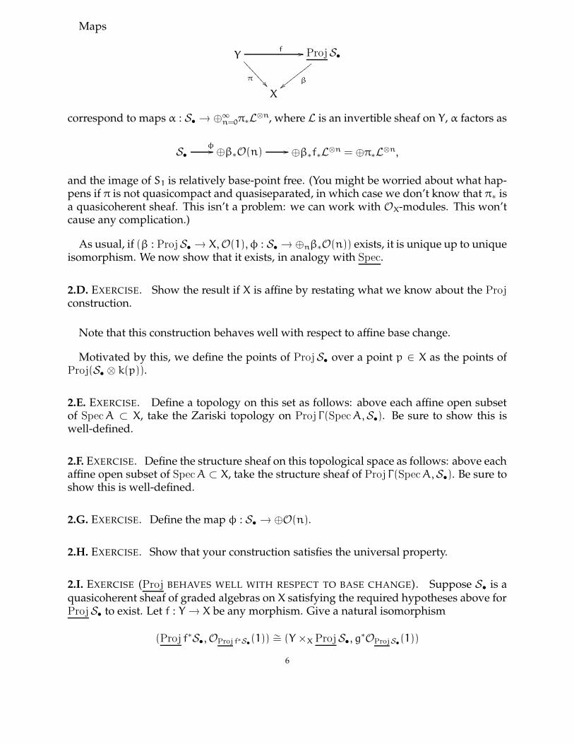
Maps

Yf

//

π��

====

====

ProjS•

β{{xx

xxxx

xxx

X

correspond to maps α : S• → ⊕∞n=0π∗L

⊗n, where L is an invertible sheaf on Y, α factors as

S•

φ// ⊕β∗O(n) // ⊕β∗f∗L

⊗n = ⊕π∗L⊗n,

and the image of S1 is relatively base-point free. (You might be worried about what hap-pens if π is not quasicompact and quasiseparated, in which case we don’t know that π∗ isa quasicoherent sheaf. This isn’t a problem: we can work with OX-modules. This won’tcause any complication.)

As usual, if (β : ProjS• → X,O(1), φ : S• → ⊕nβ∗O(n)) exists, it is unique up to uniqueisomorphism. We now show that it exists, in analogy with Spec.

2.D. EXERCISE. Show the result if X is affine by restating what we know about the Proj

construction.

Note that this construction behaves well with respect to affine base change.

Motivated by this, we define the points of ProjS• over a point p ∈ X as the points ofProj(S• ⊗ k(p)).

2.E. EXERCISE. Define a topology on this set as follows: above each affine open subsetof Spec A ⊂ X, take the Zariski topology on Proj Γ(Spec A,S•). Be sure to show this iswell-defined.

2.F. EXERCISE. Define the structure sheaf on this topological space as follows: above eachaffine open subset of Spec A ⊂ X, take the structure sheaf of Proj Γ(Spec A,S•). Be sure toshow this is well-defined.

2.G. EXERCISE. Define the map φ : S• → ⊕O(n).

2.H. EXERCISE. Show that your construction satisfies the universal property.

2.I. EXERCISE (Proj BEHAVES WELL WITH RESPECT TO BASE CHANGE). Suppose S• is aquasicoherent sheaf of graded algebras on X satisfying the required hypotheses above forProjS• to exist. Let f : Y → X be any morphism. Give a natural isomorphism

(Proj f∗S•,OProj f∗S•(1)) ∼= (Y ×X ProjS•, g

∗OProjS•(1))

6

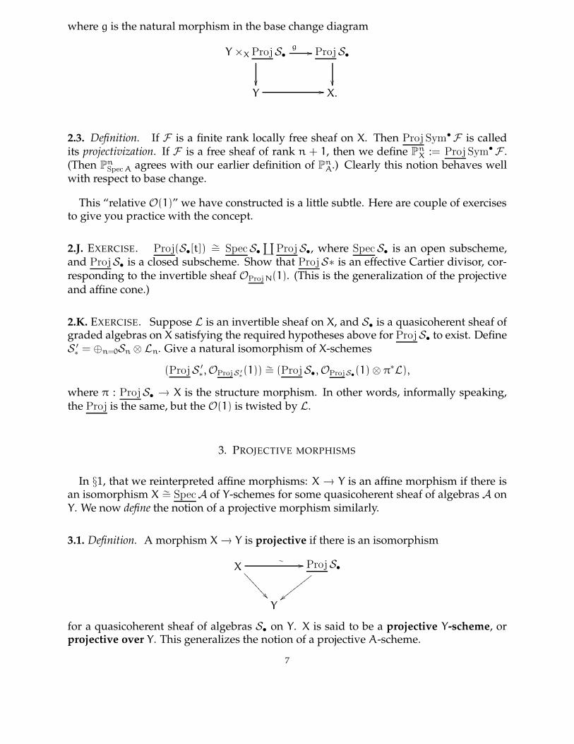
where g is the natural morphism in the base change diagram

Y ×X ProjS•

g//

��

ProjS•

��

Y // X.

2.3. Definition. If F is a finite rank locally free sheaf on X. Then Proj Sym• F is calledits projectivization. If F is a free sheaf of rank n + 1, then we define P

nX := Proj Sym• F .

(Then PnSpec A agrees with our earlier definition of P

nA.) Clearly this notion behaves well

with respect to base change.

This “relative O(1)” we have constructed is a little subtle. Here are couple of exercisesto give you practice with the concept.

2.J. EXERCISE. Proj(S•[t]) ∼= SpecS•

∐ProjS•, where Spec S• is an open subscheme,

and ProjS• is a closed subscheme. Show that ProjS∗ is an effective Cartier divisor, cor-responding to the invertible sheaf OProjN(1). (This is the generalization of the projectiveand affine cone.)

2.K. EXERCISE. Suppose L is an invertible sheaf on X, and S• is a quasicoherent sheaf ofgraded algebras on X satisfying the required hypotheses above for ProjS• to exist. DefineS ′∗ = ⊕n=0Sn ⊗ Ln. Give a natural isomorphism of X-schemes

(ProjS ′∗,OProjS ′

∗(1)) ∼= (ProjS•,OProjS•

(1) ⊗ π∗L),

where π : ProjS• → X is the structure morphism. In other words, informally speaking,the Proj is the same, but the O(1) is twisted by L.

3. PROJECTIVE MORPHISMS

In §1, that we reinterpreted affine morphisms: X → Y is an affine morphism if there isan isomorphism X ∼= SpecA of Y-schemes for some quasicoherent sheaf of algebras A onY. We now define the notion of a projective morphism similarly.

3.1. Definition. A morphism X → Y is projective if there is an isomorphism

X∼

//

��==

====

==ProjS•

||xxxx

xxxx

x

Y

for a quasicoherent sheaf of algebras S• on Y. X is said to be a projective Y-scheme, orprojective over Y. This generalizes the notion of a projective A-scheme.

7

3.2. Warnings. First, notice that O(1), an important part of the definition of Proj, is notmentioned. As a result, the notion of affine morphism is affine-local on the target, but thisnotion is not affine-local on the target. (In nice circumstances it is, as we’ll see later. We’llalso see an example where this is not.)

Second, Hartshorne gives a different definition; we are following the more general def-inition of Grothendieck. These definitions turn out to be the same in nice circumstances.

We now establish a number of properties of projective morphisms.

Note first that projective morphisms are proper. (Reason: properness is local on thebase, and we’ve seen earlier that projective A-schemes are proper over A.) Equivalently(by definition of properness!) they are separated, finite type, and universally closed.

3.A. IMPORTANT EXERCISE: FINITE MORPHISMS ARE PROJECTIVE. Show that finite mor-phisms are projective as follows. Suppose Y → X is finite, and that Y = SpecA where A

is a finite type quasicoherent sheaf on X. Describe a sheaf of graded algebras S• whereS0

∼= OX and Sn∼= A for n > 0. (What is the multiplication in this algebra?) Describe an

X-isomorphism Y ∼= ProjS•.

In particular, closed immersions are projective. We have the sequence of implicationsfor morphisms

closed immersion ⇒ finite ⇒ projective ⇒ proper.

3.B. EXERCISE. Show that a morphism (over Spec k) from a projective k-scheme to aseparated k-scheme is always projective. (Hint: the Cancellation Theorem for propertiesof morphisms.)

3.C. EXERCISE. Show that the property of a morphism being projective is preserved bybase change.

3.D. HARDER EXERCISE. Show that the property of being projective is preserved bycomposition. (Ask me for a hint. The main thing is to figure out a candidate O(1).)

The previous two exercises imply that the property of being projective is preserved byproducts: if f : X → Y and f ′ : X ′ → Y are projective, then so is f × f ′ : X × X ′ → Y × Y ′.


8


RAVI VAKIL

CONTENTS

1. Introduction 12. Definitions and proofs of key properties 53. Cohomology of line bundles on projective space 9

In these two lectures, we will define Cech cohomology and discuss its most importantproperties, although not in that order.

1. INTRODUCTION

As Γ(X, ·) is a left-exact functor, if 0 → F → G → H → 0 is a short exact sequence ofsheaves on X, then

0 → F(X) → G(X) → H(X)

is exact. We dream that this sequence continues off to the right, giving a long exact se-quence. More explicitly, there should be some covariant functors Hi (i ≥ 0) from qua-sicoherent sheaves on X to groups such that H0 = Γ , and so that there is a “long exactsequence in cohomology”.

(1) 0 // H0(X,F) // H0(X,G) // H0(X,H)

// H1(X,F) // H1(X,G) // H1(X,H) // · · ·

(In general, whenever we see a left-exact or right-exact functor, we should hope for this,and in good cases our dreams will come true. The machinery behind this is sometimescalled derived functor cohomology, which we will discuss shortly.)

Before defining cohomology groups of quasicoherent sheaves explicitly, we first de-scribe their important properties. Indeed these fundamental properties are in some waysmore important than the formal definition. The boxed properties will be the importantones.

Date: Friday, February 22 and Monday, February 25, 2008.

1

Suppose X is a separated and quasicompact A-scheme. (The separated and quasicom-pact hypotheses will be necessary in our construction.) For each quasicoherent sheaf Fon X, we will define A-modules Hi(X,F). In particular, if A = k, they are k-vector spaces.

(i) H0(X,F) = Γ(X,F) .

(ii) Each Hi is a covariant functor in the sheaf F extending the usual covariance forH0(X, ·): F → G induces Γ(X,F) → Γ(X,G).

(iii) If 0 → F → G → H → 0 is a short exact sequence of quasicoherent sheaveson X, then we have a long exact sequence (1). The maps Hi(X,F) → Hi(X,G) comefrom covariance, and similarly for Hi(X,G) → Hi(X,G). The connecting homomorphismsHi(x,H) → Hi+1(X,F) will have to be defined.

(iv) If f : X → Y is any morphism, and F is a quasicoherent sheaf on X, then there isa natural morphism Hi(Y, f∗F) → Hi(X,F) extending Γ(Y, f∗F) → Γ(X,F). We will latersee this as part of a larger story, the Leray spectral sequence. If G is a quasicoherent sheafon Y, then setting F := f∗G and using the adjunction map G → f∗f

∗G and covariance of(ii) gives a natural pullback map Hi(Y,G) → Hi(X, f∗G) (via Hi(Y,G) → Hi(Y, f∗f

∗G) →

Hi(X, f∗G)) extending Γ(Y,G) → Γ(X, f∗G). In this way, Hi is a “contravariant functor inthe space”.

(v) If f : X ↪→ Y is an affine morphism, and F is a quasicoherent sheaf on X, the naturalmap of (iv) is an isomorphism: Hi(Y, f∗F)

∼// Hi(X,F) . When f is a closed immer-

sion and Y = PNA , this isomorphism will translate calculations on arbitrary projective

A-schemes to calculations on PnA.

(vi) If X can be covered by n affines, then Hi(X,F) = 0 for i ≥ n for all F . In partic-ular, all higher (i > 0) quasicoherent cohomology groups on affine schemes vanish. Thevanishing of H1 in this case, along with the long exact sequence (iii) implies that Γ is anexact functor for quasicoherent sheaves on affine schemes, something we already knew.It is also true that if dim X = n, then Hi(X,F) = 0 for all i > n and for all F (dimensionalvanishing). We will prove this for quasiprojective A-schemes, but we won’t use this factin general, and hence won’t prove it. (A proof is given in Hartshorne (Thm. III.2.7) forderived functors, and we show in a week or two that this agrees with Cech cohomology.)

(vii) The functor Hi behaves well under direct sums, and more generally under colimits:Hi(X, lim

−→Fj) = lim

−→Hi(X,Fj) .

(viii) We will also identify the cohomology of all O(m) on PnA:

1.1. Theorem. —

• H0(PnA,OP

nA(m)) is a free A-module of rank

(

n+m

n

)

if i = 0 and m ≥ 0, and 0 otherwise.

2

• Hn(PnA,OP

nA(m)) is a free A-module of rank

(

−m−1

−n−m−1

)

if m ≤ −n − 1, and 0 otherwise.• Hi(Pn

A,OPnA(m)) = 0 if 0 < i < n.

We already have shown the first statement in an Essential Exercise (class 27 end ofsection 3).

Theorem 1.1 has a number of features that will be the first appearances of things thatwe’ll prove later.

• The cohomology of these bundles vanish above n ((vi) above)• These cohomology groups are always finitely-generated A-modules. This will be

true for all coherent sheaves on projective A-schemes (Theorem 1.2(i)).• The top cohomology group vanishes for m > −n − 1. (This is a first appearance of

Kodaira vanishing.)• The top cohomology group is one-dimensional for m = −n − 1 if A = k. This is

the first appearance of the dualizing sheaf.• There is a natural duality

Hi(X,O(m)) × Hn−i(X,O(−n − 1 − m)) → Hn(X,O(−n − 1)).

This is the first appearance of Serre duality.

Before proving these facts, let’s first use them to prove interesting things, as motivation.

By an earlier Theorem from last quarter (class 30 Corollary 3.3), for any coherent sheafF on P

nA we can find a surjection O(m)⊕j

→ F , which yields the exact sequence

(2) 0 → G → O(m)⊕j→ F → 0

for some coherent sheaf G. We can use this to prove the following.

1.2. Theorem. — (i) For any coherent sheaf F on a projective A-scheme where A is Noetherian,hi(X,F) is a coherent (finitely generated) A-module.(ii) (Serre vanishing) Furthermore, for m � 0, Hi(X,F(m)) = 0 for all i, even without Noether-ian hypotheses.

A non-Noetherian generalization of the coherence statement is given in Exercise 1.A.

Proof. Because cohomology of a closed scheme can be computed on the ambient space(see (v) above), we may immediately reduce to the case X = P

nA.

3

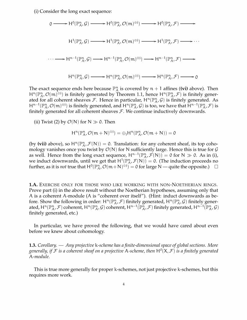
(i) Consider the long exact sequence:

0 // H0(PnA,G) // H0(Pn

A,O(m)⊕j) // H0(PnA,F) //

H1(PnA,G) // H1(Pn

A,O(m)⊕j) // H1(PnA,F) // · · ·

· · · // Hn−1(PnA,G) // Hn−1(Pn

A,O(m)⊕j) // Hn−1(PnA,F) //

Hn(PnA,G) // Hn(Pn

A,O(m)⊕j) // Hn(PnA,F) // 0

The exact sequence ends here because PnA is covered by n + 1 affines ((vi) above). Then

Hn(PnA,O(m)⊕j) is finitely generated by Theorem 1.1, hence Hn(Pn

A,F) is finitely gener-ated for all coherent sheaves F . Hence in particular, Hn(Pn

A,G) is finitely generated. AsHn−1(Pn

A,O(m)⊕j) is finitely generated, and Hn(PnA,G) is too, we have that Hn−1(Pn

A,F) isfinitely generated for all coherent sheaves F . We continue inductively downwards.

(ii) Twist (2) by O(N) for N � 0. Then

Hn(PnA,O(m + N)⊕j) = ⊕jH

n(PnA,O(m + N)) = 0

(by (vii) above), so Hn(PnA,F(N)) = 0. Translation: for any coherent sheaf, its top coho-

mology vanishes once you twist by O(N) for N sufficiently large. Hence this is true for Gas well. Hence from the long exact sequence, Hn−1(Pn

A,F(N)) = 0 for N � 0. As in (i),we induct downwards, until we get that H1(Pn

A,F(N)) = 0. (The induction proceeds nofurther, as it is not true that H0(Pn

A,O(m+N)⊕j) = 0 for large N — quite the opposite.) �

1.A. EXERCISE ONLY FOR THOSE WHO LIKE WORKING WITH NON-NOETHERIAN RINGS.Prove part (i) in the above result without the Noetherian hypotheses, assuming only thatA is a coherent A-module (A is “coherent over itself”). (Hint: induct downwards as be-fore. Show the following in order: Hn(Pn

A,F) finitely generated, Hn(PnA,G) finitely gener-

ated, Hn(PnA,F) coherent, Hn(Pn

A,G) coherent, Hn−1(PnA,F) finitely generated, Hn−1(Pn

A,G)

finitely generated, etc.)

In particular, we have proved the following, that we would have cared about evenbefore we knew about cohomology.

1.3. Corollary. — Any projective k-scheme has a finite-dimensional space of global sections. Moregenerally, if F is a coherent sheaf on a projective A-scheme, then H0(X,F) is a finitely generatedA-module.

This is true more generally for proper k-schemes, not just projective k-schemes, but thisrequires more work.

4

Here is three important consequences. They can also be shown directly, without theuse of cohomology, but with much more elbow grease.

1.B. EXERCISE. Suppose X is a projective integral scheme over an algebraically closedfield. Show that h0(X,OX) = 1. Hint: show that H0(X,OX) is a finite-dimensional k-algebra, and a domain. Hence show it is a field. (For experts: the same argument holdswith the weaker hypotheses where X is proper, geometrically connected, and reducedover an arbitrary field.)

1.C. CRUCIAL EXERCISE (PUSHFORWARDS OF COHERENTS ARE COHERENT). Supposef : X → Y is a projective morphism, and OY is coherent over itself (true in all reasonablecircumstances). Show that the pushforward of a coherent sheaf on X is a coherent sheafon Y.

Finite morphisms are affine (from the definition) and projective (shown earlier, class33/34 Exercise 3.A). We can now show that this is a characterization of finiteness.

1.4. Corollary. — If π : X → Y is projective and affine and OY is coherent, then π is finite.

In fact, more generally, if π is universally closed and affine, then π is finite, by Atiyah-Macdonald Exercise 5.35 (thanks Joe!). We won’t use this, so I won’t explain why.

Proof. By Exercise 1.C, π∗OX is coherent and hence finitely generated. �

1.D. EXERCISE. Suppose 0 → F → G → H → 0 is an exact sequence of coherent sheaveson projective X with F coherent. Show that for n � 0,

0 → H0(X,F(n)) → H0(X,G(n)) → H0(X,H(n)) → 0

is also exact. (Hint: for n � 0, H1(X,F(n)) = 0.)

2. DEFINITIONS AND PROOFS OF KEY PROPERTIES

This section could be read much later; the facts we will use are all stated in the previoussection. However, the arguments aren’t that complicated, so you may feel like readingthis right away. As you read this, you should go back and check off all the facts, to assureyourself that I’ve shown all that I’ve promised.

2.1. Cech cohomology. Cech cohomology in general settings is often defined using alimit over finer and finer covers of a space. In our algebro-geometric setting, the situationis much cleaner, and we can use a single cover.

Suppose X is quasicompact and separated, e.g. X is quasiprojective over A. In particu-lar, X may be covered by a finite number of affine open sets, and the intersection of anytwo affine open sets is also an affine open set (by separatedness, Class 17 Proposition

5

1.2). We’ll use quasicompactness and separatedness only in order to ensure these twonice properties.

Suppose F is a quasicoherent sheaf, and U = {Ui}ni=1 is a finite set of affine open sets

of X covering U. For I ⊂ {1, . . . , n} define UI = ∩i∈IUi, which is affine by the separatedhypothesis. Consider the Cech complex

(3) 0 →

M

|I| = 1

I ⊂ {1, . . . , n}

F(UI) → · · · →

M

|I| = i

I ⊂ {1, . . . , n}

F(UI) →

M

|I| = i + 1

I ⊂ {1, . . . , n}

F(UI) → · · · .

The maps are defined as follows, in terms of the summands. The map from F(UI) →

F(UJ) is 0 unless I ⊂ J, i.e. J = I ∪ {j}. If j is the kth element of J, then the map is (−1)k−1

times the restriction map resUI,UJ.

2.A. EASY EXERCISE (FOR THOSE WHO HAVEN’T SEEN ANYTHING LIKE THE CECH COM-PLEX BEFORE). Show that the Cech complex is indeed a complex, i.e. that the compositionof two consecutive arrows is 0.

Define HiU(U,F) to be the ith cohomology group of the complex (3). Note that if X is

an A-scheme, then HiU(X,F) is an A-module. We have almost succeeded in defining the

Cech cohomology group Hi, except our definition seems to depend on a choice of a coverU .

2.B. EASY EXERCISE. Show that H0U(X,F) = Γ(X,F). (Hint: use the sheaf axioms for F .)

2.C. EXERCISE. Suppose 0 → F1 → F2 → F3 → 0 is a short exact sequence of sheaveson a topological space, and U is an open cover such that on any intersection of opensubsets in U , the sections of F2 surject onto F3. Show that we get a long exact sequence ofcohomology. (Note that this applies in our case!)

2.2. Theorem/Definition. — Recall that X is quasicompact and separated. HiU(U,F) is indepen-

dent of the choice of (finite) cover {Ui}. More precisely,

(*) for all k, for any two covers {Ui} ⊂ {Vi} of size at most k, the maps Hi{Vi}

(X,F) →

Hi{Ui}

(X,F) induced by the natural maps of Cech complexes (3) are isomorphisms.

Define the Cech cohomology group Hi(X,F) to be this group.

The dependence of k in the statement is there because we will prove it by induction onk.

(For experts: maps of complexes inducing isomorphisms are called quasiisomorphisms.We are actually getting a finer invariant than cohomology out of this construction; we aregetting an element of the derived category of A-modules.)

6

Proof. We prove this by induction on k. The base case k = 1 is trivial. We need only provethe result for {Ui}

ni=1 ⊂ {Ui}

ni=0, where the case k = n is assumed known. Consider the

exact sequence of complexes

0

��

0

��

0

��

· · · //

L

|I| = i − 1

0 ∈ I ⊂ {0, . . . , n}

F(UI) //

��

L

|I| = i

0 ∈ I ⊂ {0, . . . , n}

F(UI) //

��

L

|I| = i + 1

0 ∈ I ⊂ {0, . . . , n}

F(UI) //

��

· · ·

· · · //

L

|I| = i − 1

I ⊂ {0, . . . , n}

F(UI) //

��

L

|I| = i

I ⊂ {0, . . . , n}

F(UI) //

��

L

|I| = i + 1

I ⊂ {0, . . . , n}

F(UI) //

��

· · ·

· · · //

L

|I| = i − 1

I ⊂ {1, . . . , n}

F(UI) //

��

L

|I| = i

I ⊂ {1, . . . , n}

F(UI) //

��

L

|I| = i + 1

I ⊂ {1, . . . , n}

F(UI) //

��

· · ·

0 0 0

The bottom two rows are Cech complexes with respect to two covers. We get a long exactsequence of cohomology from this short exact sequence of complexes. Thus we wishto show that the top row is exact. But the ith cohomology of the top row is preciselyHi

{Ui∩U0}i>0(Ui,F) except at step 0, where we get 0 (because the complex starts off 0 →

F(U0) → ⊕nj=1F(U0∩Uj)). So it suffices to show that higher Cech groups of affine schemes

are 0. Hence we are done by the following result. �

2.3. Theorem. — The higher Cech cohomology HiU(X,F) of an affine A-scheme X vanishes (for

any affine cover U , i > 0, and quasicoherent F ).

Serre describes this as a partition of unity argument.

Proof. We want to show that the “extended” complex

(4) 0 → F(X) → ⊕|I|=1F(UI) → ⊕|I|=2F(UI) → · · ·

(where the global sections are appended to the front) has no cohomology, i.e. is exact. Wedo this with a trick.

7

Suppose first that some Ui, say U0, is X. Then the complex is the middle row of thefollowing short exact sequence of complexes

0 // 0 //

��

⊕|I|=1,0∈IF(UI) //

��

⊕|I|=2,0∈IF(UI) //

��

· · ·

0 // F(X) //

��

⊕|I|=1F(UI) //

��

⊕|I|=2F(UI) //

��

· · ·

0 // F(X) // ⊕|I|=1,0/∈IF(UI) // ⊕|I|=2,0/∈IF(UI) // · · ·

The top row is the same as the bottom row, slid over by 1. The corresponding long exactsequence of cohomology shows that the central row has vanishing cohomology. (Topo-logical experts will recognize this as a mapping cone construction.)

We next prove the general case by sleight of hand. Say X = Spec R. We wish to showthat the complex of A-modules (4) is exact. It is also a complex of R-modules, so wewish to show that the complex of R-modules (4) is exact. To show that it is exact, itsuffices to show that for a cover of Spec R by distinguished open sets D(fi) (1 ≤ i ≤ r)(i.e. (f1, . . . , fr) = 1 in R) the complex is exact. (Translation: exactness of a sequence ofsheaves may be checked locally.) We choose a cover so that each D(fi) is contained insome Uj = Spec Aj. Consider the complex localized at fi. As

Γ(Spec A,F)f = Γ(Spec(Aj)f,F)

(as this is one of the definitions of a quasicoherent sheaf), as Uj ∩ D(fi) = D(fi), we are inthe situation where one of the Ui’s is X, so we are done. �

We have now proved properties (i)–(iii) of the previous section.

2.D. EXERCISE (PROPERTY (v)). Suppose f : X → Y is an affine morphism, and Y isa quasicompact and separated A-scheme (and hence X is too, as affine morphisms areboth quasicompact and separated). If F is a quasicoherent sheaf on X, describe a naturalisomorphism Hi(Y, f∗F) ∼= Hi(X,F). (Hint: if U is an affine cover of Y, “f−1(U)” is anaffine cover X. Use these covers to compute the cohomology of F .)

2.E. EXERCISE (PROPERTY (iv)). Suppose f : X → Y is any quasicompact separatedmorphism, F is a quasicoherent sheaf on X, and Y is a quasicompact quasiseparated A-scheme. The hypotheses on f ensure that f∗F is a quasicoherent sheaf on Y. Describe anatural morphism Hi(Y, f∗F) → Hi(X,F) extending Γ(Y, f∗F) → Γ(X,F).

2.F. UNIMPORTANT EXERCISE. Prove Property (vii) of the previous section.

2.4. Useful facts about cohomology for k-schemes.8

2.G. EXERCISE (COHOMOLOGY AND CHANGE OF BASE FIELD). Suppose X is a projectivek-scheme, and F is a coherent sheaf on X. Show that

h0(X,F) = h0(X ×Spec k Spec K,F ⊗k K)

where K/k is any field extension. Here F ⊗k k means the pullback of F to X×Spec k Spec K.Note: the two sides of this equality are dimensions of vector spaces over different fields!(This is useful for relating facts about k-schemes to facts about schemes over algebraicallyclosed fields.)

2.5. Theorem. — Suppose X is a projective k-scheme, and F is a quasicoherent sheaf on X. ThenHi(X,F) = 0 for i > dim X.

In other words, cohomology vanishes above the dimension of X. We will later showthat this is true when X is a quasiprojective k-scheme.

Proof. Suppose X ↪→ PN, and let n = dim X. We show that X may be covered by n affine

open sets. A key Exercise from a couple of months ago shows that there are n effectiveCartier divisors on P

N such that their complements U0, . . . , Un cover X. Then Ui is affine,so Ui ∩ X is affine, and thus we have covered X with n affine open sets. �

Remark. We actually need n affine open sets to cover X, but I don’t see an easy way toprove it. One way of proving it is by showing that the complement of an affine set isalways pure codimension 1.

3. COHOMOLOGY OF LINE BUNDLES ON PROJECTIVE SPACE

We will finally prove the last promised basic fact about cohomology, property (viii) of§1, Theorem 1.1.

We saw earlier (Essential Exercise in class 27, end of section 3, and the ensuing discus-sion) that H0(Pn

A,OPnA(m)) should be interpreted as the homogeneous degree m polyno-

mials in x0, . . . , xn (with A-coefficients). Similarly, Hn(PnA,OP

nA(m)) should be interpreted

as the homogeneous degree m Laurent polynomials in x0, . . . , xn, where in each mono-mial, each xi appears with degree at most −1.

Proof of Theorem 1.1. As stated above, we showed the H0 case earlier.

Rather than consider O(m) for various m, we consider them all at once, by consideringF = ⊕mO(m).

We take the standard cover U0 = D(x0), . . . , Un = D(xn) of PnA. Notice that if I ⊂

{1, . . . , n}, then F(UI) corresponds to the Laurent monomials where each xi for i /∈ I

appears with non-negative degree.

We first consider the Hn statement. Hn(PnA,F) is the cokernel of the surjection

⊕ni=0F(U{1,...,n}−{i}) → FU{1,...,n}

9

i.e.⊕n

i=0A[x0, . . . , xn, x−10 , . . . , ^x−1

i , . . . x−1n ] → A[x0, . . . , xn, x−1

0 , . . . , x−1n ].

This cokernel is precisely as described.

We last consider the Hi statement (0 < i < n). (Strangely, the vanishing of these Hi isthe hardest part of the Theorem.) We prove this by induction on n. The cases n = 0 and 1

are trivial. Consider the exact sequence of quasicoherent sheaves:

0 // F×xn

// F // F ′ // 0

where F ′ is analogous sheaf on the hyperplane xn = 0 (isomorphic to Pn−1A ). (This exact

sequence is just the direct sum over all m of the exact sequence

0 // OPnA(m − 1)

×xn// OP

nA(m) // O

Pn−1A

(m) // 0 ,

which in turn is obtained by twisting the closed subscheme exact sequence

0 // OPnA(−1)

×xn// OP

nA

// OP

n−1A

// 0

by OPnA(m).)

The long exact sequence in cohomology yields

0 // H0(PnA,F)

×xn// H0(Pn

A,F) // H0(Pn−1A ,F ′)

// H1(PnA,F)

×xn// H1(Pn

A,F) // H1(Pn−1A ,F ′)

. . . // Hn−1(PnA,F)

×xn// Hn−1(Pn

A,F) // Hn−1(Pn−1A ,F ′)

// Hn(PnA,F)

×xn// Hn(Pn

A,F) // 0

.

We will now show that this gives an isomorphism

(5) ×xn : Hi(PnA,F)

∼// Hi(Pn

A,F)

for 0 < i < n. The inductive hypothesis gives us this except for i = 1 and i = n−1, wherewe have to be more careful. For the first, note that H0(Pn

A,F) // H0(Pn−1A ,F ′) is sur-

jective: this map corresponds to taking the set of all polynomials in x0, . . . , xn, and settingxn = 0. The last is slightly more subtle: Hn−1(Pn−1

A ,F ′) → Hn(PnA,F) is injective, and cor-

responds to taking a Laurent polynomial in x0, . . . , xn−1 (where in each monomial, eachxi appears with degree at most −1) and multiplying by x−1

n , which indeed describes thekernel of Hn(Pn

A,F)×xn

// Hn(PnA,F) . (This is a worthwhile calculation! See Exercise 3.A

below.) We have thus established (5) above.

We will now show that the localization Hi(PnA,F)xn

= 0. (Here’s what we mean bylocalization. Notice Hi(Pn

A,F) is naturally a module over A[x0, . . . , xn] — we know how

10

to multiply by elements of A, and by (5) we know how to multiply by xi. Then we localizethis at xn to get an A[x0, . . . , xn]xn

-module.) This means that each element α ∈ Hi(PnA,F)

is killed by some power of xi. But by (5), this means that α = 0, concluding the proof ofthe theorem.

Consider the Cech complex computing Hi(PnA,F). Localize it at xn. Localization and

cohomology commute (basically because localization commutes with operations of tak-ing quotients, images, etc.), so the cohomology of the new complex is Hi(Pn

A,F)xn. But

this complex computes the cohomology of Fxnon the affine scheme Un, and the higher

cohomology of any quasicoherent sheaf on an affine scheme vanishes (by Theorem 2.3which we’ve just proved — in fact we used the same trick there), so Hi(Pn

A,F)xn= 0 as

desired. �

3.A. EXERCISE. Verify that Hn−1(Pn−1A ,F ′) → Hn(Pn

A,F) is injective (likely by verifyingthat it is the map on Laurent monomials we claimed above).


11


RAVI VAKIL

CONTENTS

1. Application of cohomology: Hilbert polynomials and functions, Riemann-Roch, degrees, and arithmetic genus 1

1. APPLICATION OF COHOMOLOGY: HILBERT POLYNOMIALS AND FUNCTIONS,RIEMANN-ROCH, DEGREES, AND ARITHMETIC GENUS

We have now seen some powerful uses of Cech cohomology, to prove things aboutspaces of global sections, and to prove Serre vanishing. We will now see some classicalconstructions come out very quickly and cheaply.

In this section, we will work over a field k. Define hi(X,F) := dimk Hi(X,F).

Suppose F is a coherent sheaf on a projective k-scheme X. Define the Euler character-istic

χ(X,F) :=

dim X∑

i=0

(−1)ihi(X,F).

We will see repeatedly here and later that Euler characteristics behave better than indi-vidual cohomology groups. As one sign, notice that for fixed n, and m ≥ 0,

h0(Pnk ,O(m)) =

(

n + m

m

)

=(m + 1)(m + 2) · · · (m + n)

n!.

Notice that the expression on the right is a polynomial in m of degree n. (For laterreference, notice also that the leading coefficient is mn/n!.) But it is not true that

h0(Pnk ,O(m)) =

(m + 1)(m + 2) · · · (m + n)

n!

for all m — it breaks down for m ≤ −n − 1. Still, you can check that

χ(Pnk ,O(m)) =

(m + 1)(m + 2) · · · (m + n)

n!.

So one lesson is this: if one cohomology group (usual the top or bottom) behaves well ina certain range, and then messes up, likely it is because (i) it is actually the Euler char-acteristic which is behaving well always, and (ii) the other cohomology groups vanish inthat range.

Date: Wednesday, February 27, 2008.

1

In fact, we will see that it is often hard to calculate cohomology groups (even h0), butit can be easier calculating Euler characteristics. So one important way of getting a holdof cohomology groups is by computing the Euler characteristics, and then showing thatall the other cohomology groups vanish. Hence the ubiquity and importance of vanishingtheorems. (A vanishing theorem usually states that a certain cohomology group vanishesunder certain conditions.) We will see this in action when discussing curves.

The following exercise shows another way in which Euler characteristic behaves well:it is additive in exact sequences.

1.A. EXERCISE. Show that if 0 → F → G → H → 0 is an exact sequence of coherentsheaves on X, then χ(X,G) = χ(X,F) + χ(X,H). (Hint: consider the long exact sequencein cohomology.) More generally, if

0 → F1 → · · · → Fn → 0

is an exact sequence of sheaves, show thatn∑

i=1

(−1)iχ(X,Fi) = 0.

1.1. The Riemann-Roch Theorem for line bundles on a nonsingular projective curve.Suppose L is an invertible sheaf on a projective curve C over k. We tentatively define thedegree of L as follows. Let s be a non-zero rational section on C. Let D be the divisor ofzeros and poles of s:

D :=∑

p∈C

vp(s)[p]

Then define degL := deg D =∑

vp(s) deg p. Here deg p is the degree of the residue fieldof OC at p, i.e. dim kOp = deg p. It isn’t yet clear degL is well-defined: a priori it dependson the choice of s. Nonetheless you should prove the following.

1.B. EXERCISE: THE RIEMANN-ROCH THEOREM FOR LINE BUNDLES ON A NONSINGULARPROJECTIVE CURVE. Show that

χ(C,L) = degL + χ(C,OC).

Here is a possible hint. Suppose p ∈ C is a closed point of C, of degree d. Then twistingthe closed exact sequence

0 → OC(−p) → OC → Op → 0

by L (as ⊗L is an exact functor) we obtain0 → L(−p) → L → Op → 0

(where we are using a non-canonical isomorphism L|p ∼= OC|p = Op). Use the additivityof χ in exact sequences to show that the result is true for L if and only if it is true forL(−p). The result is also clearly true for L = O. Then argue by “induction” that it is truefor all L.

2

In particular, degL is well-defined!

1.C. EXERCISE. If L and M are two line bundles on a nonsingular projective curve C,show that degL⊗M = degL + degM. (Hint: choose rational sections of L and M.)

In fact we could have defined the degree of a line bundle L on a nonsingular projectivecurve C to be χ(C,L)−χ(C,OC). Then Riemann-Roch would be true by definition; but wewould still want to relate this notion of degree to the classical notion of zeros and poles,which we would do by the argument in the previous paragraph. Otherwise, for example,Exercise 1.C isn’t obvious from the cohomological definition.

Definition. Suppose C is a reduced projective curve (pure dimension 1, over a field k).If L is a line bundle on C, define degL = χ(C,L) − χ(C,OC). If C is irreducible, and F isa coherent sheaf on C, define the rank of F , denoted rankF , to be its rank at the genericpoint of C.

1.D. EASY EXERCISE. Show that the rank is additive in exact sequences: if 0 → F → G →H → 0 is an exact sequence of coherent sheaves, show that rankF − rankG + rankH = 0.

Definition. Define

(1) degF = χ(C,F) − (rankF)χ(C,OC).

If F is a line bundle, we can drop the hypothesis of irreducibility in the definition.

This generalizes the notion of the degree of a line bundle on a nonsingular curve.

1.E. EASY EXERCISE. Show that degree is additive in exact sequences.

The statement (1) is often called Riemann-Roch for coherent sheaves (or vector bundles)on a projective curve.

If F is a coherent sheaf on X, define the Hilbert function of F :

hF(n) := h0(X,F(n)).

The Hilbert function of X is the Hilbert function of the structure sheaf. The ancientswere aware that the Hilbert function is “eventually polynomial”, i.e. for large enough n,it agrees with some polynomial, called the Hilbert polynomial (and denoted pF(n) orpX(n)). This polynomial contains lots of interesting geometric information, as we willsoon see. In modern language, we expect that this “eventual polynomiality” arises be-cause the Euler characteristic should be a polynomial, and that for n � 0, the highercohomology vanishes. This is indeed the case, as we now verify.

1.2. Theorem. — If F is a coherent sheaf on a projective k-scheme X ↪→ Pnk , χ(X,F(m)) is a

polynomial of degree equal to dim SuppF . Hence by Serre vanishing (Theorem 1.2(ii) in the class3

35/36 notes), for m � 0, h0(X,F(m)) is a polynomial of degree dim SuppF . In particular, form � 0, h0(X,OX(m)) is polynomial with degree = dim X.

Here OX(m) is the restriction or pullback of OPnk(1). Both the degree of the 0 polynomial

and the dimension of the empty set is defined to be −1. In particular, the only coherentsheaf Hilbert polynomial 0 is the zero-sheaf.

Proof. Define pF(m) = χ(X,F(m)). We will show that pF(m) is a polynomial of thedesired degree.

Step 1. Assume first that k is infinite. (This is one of those cases where even if youare concerned with potentially arithmetic questions over some non-algebraically closedfield like Fp, you are forced to consider the “geometric” situation where the base field isalgebraically closed.)

F has a finite number of associated points. Then there is a hyperplane x = 0 (x ∈

Γ(X,O(1))) missing this finite number of points. (This is where we use the algebraic clo-sure, or more precisely, the infinitude of k.)

Then the map F(−1)×x

// F is injective (on any affine open subset, F corresponds toa module, and x is not a zero-divisor on that module, as it doesn’t vanish at any associatedpoint of that module). Thus we have a short exact sequence

(2) 0 → F(−1) → F → G → 0

where G is a coherent sheaf.

1.F. EXERCISE. Show that Supp G = SuppF ∩ V(x).

Hence dim Supp G = dim SuppF − 1 by Krull’s Principal Ideal Theorem unless F = 0

(in which case we already know the result, so assume this is not the case).

Twisting (2) by O(m) yields

0 → F(m − 1) → F(m) → G(m) → 0

Euler characteristics are additive in exact sequences, from which pF(m) − pF(m − 1) =

pG(m). Now pG(m) is a polynomial of degree dim SuppF − 1.

The result follows from a basic fact about polynomials.

1.G. EXERCISE. Suppose f and g are functions on the integers, f(m + 1) − f(m) = g(m)

for all m, and g(m) is a polynomial of degree d ≥ 0. Show that f is a polynomial of degreed + 1.

Step 2: k finite.4

1.H. EXERCISE. Complete the proof using Exercise 2.G from the notes from class 35/36(on cohomology and change of base field), using K = k.

�

Definition. pF(m) was defined in the above proof. If X ⊂ Pn is a projective k-scheme,define pX(m) := pOX

(m).

Example 1. pPn(m) =(

m+n

n

)

, where we interpret this as the polynomial (m + 1) · · · (m +

n)/n!.

Example 2. Suppose H is a degree d hypersurface in Pn. Then from the closed sub-scheme exact sequence

0 → OPn(−d) → OPn → OH → 0,

we havepH(m) = pPn(m) − pPn(m − d) =

(

m + n

n

)

−

(

m + n − d

n

)

.

1.I. EXERCISE. Show that the twisted cubic (in P3) has Hilbert polynomial 3m + 1.

1.J. EXERCISE. Find the Hilbert polynomial for the dth Veronese embedding of Pn (i.e.the closed immersion of Pn in a bigger projective space by way of the line bundle O(d)).

From the Hilbert polynomial, we can extract many invariants, of which two are par-ticularly important. The first is the degree. Classically, the degree of a complex projectivevariety of dimension n was defined as follows. We slice the variety with n generally cho-sen hyperplane. Then the intersection will be a finite number of points. The degree isthis number of points. Of course, this requires showing all sorts of things. Instead, wewill define the degree of a projective k-scheme of dimension n to be leading coefficient of theHilbert polynomial (the coefficient of mn) times n!.

Using the examples above, we see that the degree of Pn in itself is 1. The degree of thetwisted cubic is 3.

1.K. EXERCISE. Show that the degree is always an integer. Hint: by induction, show thatany polynomial in m of degree k taking on only integral values must have coefficient ofmk an integral multiple of 1/k!. Hint for this: if f(x) takes on only integral values and isof degree k, then f(x + 1) − f(x) takes on only integral values and is of degree k − 1.

1.L. EXERCISE. Show that the degree of a degree d hypersurface is d (preventing anotational crisis).

1.M. EXERCISE. Suppose a curve C is embedded in projective space via an invertiblesheaf of degree d. In other words, this line bundle determines a closed immersion. Show

5

that the degree of C under this embedding is d (preventing another notational crisis).(Hint: Riemann-Roch, Exercise 1.B.)

1.N. EXERCISE. Show that the degree of the dth Veronese embedding of Pn is dn.

1.O. EXERCISE (BEZOUT’S THEOREM). Suppose X is a projective scheme of dimensionat least 1, and H is a degree d hypersurface not containing any associated points of X.(For example, if X is a projective variety, then we are just requiring H not to contain anyirreducible components of X.) Show that deg H ∩ X = d deg X.

This is a very handy theorem! For example: if two projective plane curves of degree m

and degree n share no irreducible components, then they intersect in mn points, countedwith appropriate multiplicity. The notion of multiplicity of intersection is just the degreeof the intersection as a k-scheme.

We trot out a useful example we have used before: let k = Q, and consider the parabolax = y2. We intersect it with the four lines, x = 1, x = 0, x = −1, and x = 2, and see thatwe get 2 each time (counted with the same convention as with the last time we saw thisexample).

If we intersect it with y = 2, we only get one point — but that’s of course because thisisn’t a projective curve, and we really should be doing this intersection on P2

k — and inthis case, the conic meets the line in two points, one of which is “at ∞”.

]

1.P. EXERCISE. Show that the degree of the d-fold Veronese embedding of Pn is dn

in a different way (from Exercise 1.N) as follows. Let vd : Pn → PN be the Veroneseembedding. To find the degree of the image, we intersect it with n hyperplanes in PN

(scheme-theoretically), and find the number of intersection points (counted with multi-plicity). But the pullback of a hyperplane in PN to Pn is a degree d hypersurface. Performthis intersection in Pn, and use Bezout’s theorem (Exercise 1.O).

There is another nice important of information residing in the Hilbert polynomial. No-tice that pX(0) = χ(X,OX), which is an intrinsic invariant of the scheme X, which does notdepend on the projective embedding.

Imagine how amazing this must have seemed to the ancients: they defined the Hilbertfunction by counting how many “functions of various degrees” there are; then they no-ticed that when the degree gets large, it agrees with a polynomial; and then when theyplugged 0 into the polynomial — extrapolating backwards, to where the Hilbert functionand Hilbert polynomials didn’t agree — they found a magic invariant!

Now we can finally see a nonsingular curve over an algebraically closed field that isprovably not P1! Note that the Hilbert polynomial of P1 is (m+1)/1 = m+1, so χ(OP1) =

6

1. Suppose C is a degree d curve in P2. Then the Hilbert polynomial of C is

pP2(m) − pP2(m − d) = (m + 1)(m + 2)/2 − (m − d + 1)(m − d + 2)/2.

Plugging in m = 0 gives us −(d2 − 3d)/2. Thus when d > 2, we have a curve that cannotbe isomorphic to P1! (I think I gave you an earlier exercise that there is a nonsingulardegree d curve.)

Now from 0 → OP2(−d) → OP2 → OC → 0, using h1(OP2(d)) = 0, we have thath0(C,OC) = 1. As h0 − h1 = χ, we have

h1(C,OC) = (d − 1)(d − 2)/2.

Motivated by geometry, we define the arithmetic genus of a scheme X as 1−χ(X,OX). Thisis sometimes denoted pa(X). In the case of nonsingular complex curves, this correspondsto the topological genus. For irreducible reduced curves (or more generally, curves withh0(X,OX) ∼= k), pa(X) = h1(X,OX). (In higher dimension, this is a less natural notion.)

We thus now have examples of curves of genus 0, 1, 3, 6, 10, . . . (corresponding to degree1 or 2, 3, 4, 5, . . . ).

This begs some questions, such as: are there curves of other genera? (We’ll see soonthat the answer is yes.) Are there other genus 1 curves? (Not if k is algebraically closed,but yes otherwise.) Do we have all the curves of genus 3? (Almost all, but not quite.) Dowe have all the curves of genus 6? (We’re missing most of them.)

Caution: The Euler characteristic of the structure sheaf doesn’t distinguish betweenisomorphism classes of nonsingular projective schemes over algebraically closed fields— for example, P1 × P1 and P2 both have Euler characteristic 1, but are not isomorphic —Pic P2 ∼= Z while Pic P1 × P1 ∼= Z ⊕ Z.

Important Remark. We can restate the Riemann-Roch formula for curves (Exercise 1.B)as:

h0(C,L) − h1(C,L) = degL − pa + 1.

This is the most common formulation of the Riemann-Roch formula.

If C is a nonsingular irreducible projective complex curve, then the correspondingcomplex-analytic object, a compact Riemann surface, has a notion called the genus g, whichis the number of holes. It turns out that g = pa in this case, and for this reason, we willoften write g for pa when discussing nonsingular (projective irreducible) curves, over anyfield.

1.3. Complete intersections. We define a complete intersection in Pn as follows. Pn is acomplete intersection in itself. A closed subscheme Xr ↪→ Pn of dimension r (with r < n)is a complete intersection if there is a complete intersection Xr+1, and Xr is an effectiveCartier divisor in class OXr+1

(d).

7

1.Q. EXERCISE. Show that if X is a complete intersection of dimension r in Pn, thenHi(X,OX(m)) = 0 for all 0 < i < r and all m. Show that if r > 0, then H0(Pn,O(m)) →H0(X,O(m)) is surjective. (Hint: long exact sequences.)

Now Xr is the divisor of a section of OXr+1(m) for some m. But this section is the

restriction of a section of O(m) on Pn. Hence Xr is the scheme-theoretic intersection ofXr+1 with a hypersurface. Thus inductively Xr is the scheme-theoretic intersection of n−r

hypersurfaces. (By Bezout’s theorem, Exercise 1.O, deg Xr is the product of the degree ofthe defining hypersurfaces.)

1.R. EXERCISE (COMPLETE INTERSECTIONS ARE CONNECTED). Show that complete in-tersections of positive dimension are connected. (Hint: show h0(X,OX) = 1.)

1.S. EXERCISE. Find the genus of the intersection of 2 quadrics in P3. (We get curves ofmore genera by generalizing this! At this point we need to worry about whether thereare any nonsingular curves of this form. We can check this by hand, but later Bertini’sTheorem will save us this trouble.)

1.T. EXERCISE. Show that the rational normal curve of degree d in Pd is not a completeintersection if d > 2. (Hint: If it were the complete intersection of d − 1 hypersurfaces,what would the degree of the hypersurfaces be? Why could none of the degrees be 1?)

1.U. EXERCISE. Show that the union of 2 distinct planes in P4 is not a complete intersec-tion. Hint: it is connected, but you can slice with another plane and get something notconnected (see Exercise 1.R).

This is another important scheme in algebraic geometry that is an example of manysorts of behavior. We will see more of it later!


8


RAVI VAKIL

CONTENTS

1. A useful very general fact from homological algebra 12. Higher direct image sheaves 13. Fun applications of the higher pushforward 4

1. A USEFUL VERY GENERAL FACT FROM HOMOLOGICAL ALGEBRA

Here is a fact that is very useful, because it applies in so many situations.

1.A. IMPORTANT EXERCISE IN ABSTRACT NONSENSE. Suppose F : A → B is a covariantadditive functor from one abelian category to another. Suppose C• is a complex in A.

(a) Describe a natural morphism FH•→ H•F.

(b) If F is exact, show that the morphism of (a) is an isomorphism.

If this makes your head spin, you may prefer to think of it in the following specificcase, where both A and B are the category of A-modules, and F is · ⊗ N for some fixedN-module. Your argument in this case will translate without change to yield a solution toExercise 1.A. If ⊗N is exact, then N is called a flat A-module.

For example, localization is exact, so S−1A is a flat A-algebra for all multiplicative setsS. Thus taking cohomology of a complex of A-modules commutes with localization —something you could verify directly.

2. HIGHER DIRECT IMAGE SHEAVES

Cohomology groups were defined for X → Spec A where the structure morphism isquasicompact and separated; for any quasicoherent F on X, we defined Hi(X,F). We’llnow define a “relative” version of this notion, for quasicompact and separated mor-phisms π : X → Y: for any quasicoherent F on X, we’ll define Riπ∗F , a quasicoherentsheaf on Y.

Date: Friday, February 29, 2008.

1

We have many motivations for doing this. In no particular order:

(1) It “globalizes” what we did before.(2) If 0 → F → G → H → 0 is a short exact sequence of quasicoherent sheaves on X,

then we know that 0 → π∗F → π∗G → π∗H is exact, and higher pushforwards willextend this to a long exact sequence.

(3) We’ll later see that this will show how cohomology groups vary in families, espe-cially in “nice” situations. Intuitively, if we have a nice family of varieties, and afamily of sheaves on them, we could hope that the cohomology varies nicely infamilies, and in fact in “nice” situations, this is true. (As always, “nice” usuallymeans “flat”, whatever that means.)

All of the important properties of cohomology described earlier will carry over to thismore general situation. Best of all, there will be no extra work required.

In the notation Rjf∗F for higher pushforward sheaves, the “R” stands for “right derivedfunctor”, and corresponds to the fact that we get a long exact sequence in cohomologyextending to the right (from the 0th terms). Later this year, we will see that in goodcircumstances, if we have a left-exact functor, there is be a long exact sequence going offto the right, in terms of right derived functors. Similarly, if we have a right-exact functor(e.g. if M is an A-module, then ⊗AM is a right-exact functor from the category of A-modules to itself), there may be a long exact sequence going off to the left, in terms of leftderived functors.

Suppose π : X → Y, and F is a quasicoherent sheaf on X. For each Spec A ⊂ Y, we haveA-modules Hi(π−1(Spec A),F). We will show that these patch together to form a quasi-coherent sheaf. We need check only one fact: that this behaves well with respect to takingdistinguished open sets. In other words, we must check that for each f ∈ A, the natu-ral map Hi(π−1(Spec A),F) → Hi(π−1(Spec A),F)f (induced by the map of spaces in theopposite direction — Hi is contravariant in the space) is precisely the localization ⊗AAf.But this can be verified easily: let {Ui} be an affine cover of π−1(Spec A). We can computeHi(π−1(Spec A),F) using the Cech complex. But this induces a cover Spec Af in a naturalway: If Ui = Spec Ai is an affine open for Spec A, we define U ′

i = Spec(Ai)f. The resultingCech complex for Spec Af is the localization of the Cech complex for Spec A. As tak-ing cohomology of a complex commutes with localization (as discussed in Exercise 1.A),we have defined a quasicoherent sheaf on Y by one of our definitions of quasicoherentsheaves by Definition 2’ of a quasicoherent sheaf.

Define the ith higher direct image sheaf or the ith (higher) pushforward sheaf to bethis quasicoherent sheaf.

2.1. Theorem. —

(a) R0π∗F is canonically isomorphic to π∗F .(b) Riπ∗ is a covariant functor from the category of quasicoherent sheaves on X to the category

of quasicoherent sheaves on Y, and a contravariant functor in Y-schemes X.2

(c) (the long exact sequence of higher pushforward sheaves) A short exact sequence0 → F → G → H → 0 of sheaves on X induces a long exact sequence

0 // R0π∗F// R0π∗G

// R0π∗H//

R1π∗F// R1π∗G

// R1π∗H// · · ·

of sheaves on Y.(d) (projective pushforwards of coherent are coherent) If π is a projective morphism and OY is

coherent on Y (this hypothesis is automatic for Y locally Noetherian), and F is a coherentsheaf on X, then for all i, Riπ∗F is a coherent sheaf on Y.

Proof. Because it suffices to check each of these results on affine open sets, they all followfrom the analogous statements in Cech cohomology. �

The following result is handy, and essentially immediate from our definition.

2.A. EXERCISE. Show that if π is affine, then for i > 0, Riπ∗F = 0.

Remark. This is in fact a characterization of affineness. Serre’s criterion for affinenessstates that if f is quasicompact and separated, then f is affine if and only if f∗ is an exactfunctor from the category of quasicoherent sheaves on X to the category of quasicoherentsheaves on Y. exact on the category of quasicoherent sheaves (EGA II.5.2). We won’t usethis fact.

2.B. EXERCISE (HIGHER PUSHFORWARDS AND COMMUTATIVE DIAGRAMS). (a) Supposef : Z → Y is any morphism, and π : X → Y as usual is quasicompact and separated.Suppose F is a quasicoherent sheaf on X. Let

Wf ′

//

π ′

��

X

π

��

Zf

// Y

is a fiber diagram. Describe a natural morphism f∗(Riπ∗F) → Riπ ′

∗(f ′)∗F of sheaves on

Z. (Hint: Exercise 1.A.)(b) If f : Z → Y is an affine morphism, and for a cover Spec Ai of Y, where f−1(Spec Ai) =Spec Bi, Bi is a flat A-algebra, and the diagram in (a) is a fiber square, show that the naturalmorphism of (a) is an isomorphism. (You can likely generalize this immediately, but thiswill lead us into the concept of flat morphisms, and we’ll hold off discussing this notionfor a while.)

A useful special case of (a) if the following.

2.C. EXERCISE. Show that if y ∈ Y, there is a natural morphism Hi(Y, f∗F)y → Hi(f−1(y),F |f−1(y)).(Hint: if you take a complex, and tensor it with a module, and take cohomology, there is

3

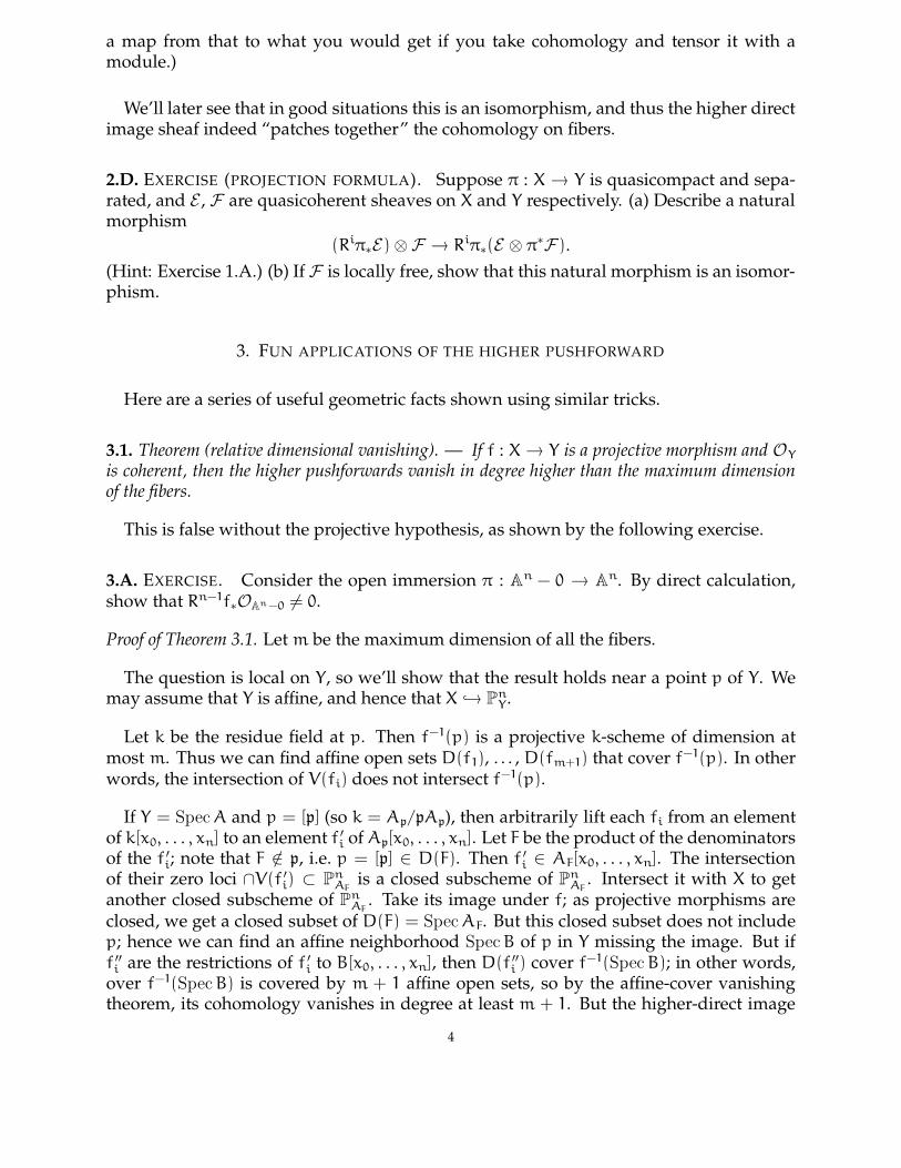
a map from that to what you would get if you take cohomology and tensor it with amodule.)

We’ll later see that in good situations this is an isomorphism, and thus the higher directimage sheaf indeed “patches together” the cohomology on fibers.

2.D. EXERCISE (PROJECTION FORMULA). Suppose π : X → Y is quasicompact and sepa-rated, and E , F are quasicoherent sheaves on X and Y respectively. (a) Describe a naturalmorphism

(Riπ∗E) ⊗F → Riπ∗(E ⊗ π∗F).

(Hint: Exercise 1.A.) (b) If F is locally free, show that this natural morphism is an isomor-phism.

3. FUN APPLICATIONS OF THE HIGHER PUSHFORWARD

Here are a series of useful geometric facts shown using similar tricks.

3.1. Theorem (relative dimensional vanishing). — If f : X → Y is a projective morphism and OY

is coherent, then the higher pushforwards vanish in degree higher than the maximum dimensionof the fibers.

This is false without the projective hypothesis, as shown by the following exercise.

3.A. EXERCISE. Consider the open immersion π : An − 0 → A

n. By direct calculation,show that Rn−1f∗OAn−0 6= 0.

Proof of Theorem 3.1. Let m be the maximum dimension of all the fibers.

The question is local on Y, so we’ll show that the result holds near a point p of Y. Wemay assume that Y is affine, and hence that X ↪→ P

nY .

Let k be the residue field at p. Then f−1(p) is a projective k-scheme of dimension atmost m. Thus we can find affine open sets D(f1), . . . , D(fm+1) that cover f−1(p). In otherwords, the intersection of V(fi) does not intersect f−1(p).

If Y = Spec A and p = [p] (so k = Ap/pAp), then arbitrarily lift each fi from an elementof k[x0, . . . , xn] to an element f ′

i of Ap[x0, . . . , xn]. Let F be the product of the denominatorsof the f ′

i; note that F /∈ p, i.e. p = [p] ∈ D(F). Then f ′

i ∈ AF[x0, . . . , xn]. The intersectionof their zero loci ∩V(f ′

i) ⊂ PnAF

is a closed subscheme of PnAF

. Intersect it with X to getanother closed subscheme of P

nAF

. Take its image under f; as projective morphisms areclosed, we get a closed subset of D(F) = Spec AF. But this closed subset does not includep; hence we can find an affine neighborhood Spec B of p in Y missing the image. But iff ′′

i are the restrictions of f ′

i to B[x0, . . . , xn], then D(f ′′

i ) cover f−1(Spec B); in other words,over f−1(Spec B) is covered by m + 1 affine open sets, so by the affine-cover vanishingtheorem, its cohomology vanishes in degree at least m + 1. But the higher-direct image

4

sheaf is computed using these cohomology groups, hence the higher direct image sheafRif∗F vanishes on Spec B too. �

3.B. IMPORTANT EXERCISE. Use a similar argument to prove semicontinuity of fiber di-mension of projective morphisms: suppose π : X → Y is a projective morphism where OY iscoherent. Show that {y ∈ Y : dim f−1(y) > k} is a Zariski-closed subset. In other words, thedimension of the fiber “jumps over Zariski-closed subsets”. (You can interpret the casek = −1 as the fact that projective morphisms are closed.) This exercise is rather importantfor having a sense of how projective morphisms behave!

Here is another handy theorem, that is proved by a similar argument. We know thatfinite morphisms are projective, and have finite fibers. Here is the converse.

3.2. Theorem (projective + finite fibers = finite). — Suppose π : X → Y is such that OY iscoherent. Then π is projective and finite fibers if and only if it is finite. Equivalently, π is projectiveand quasifinite if and only it is finite.

(Recall that quasifinite = finite fibers + finite type. But projective includes finite type.)

It is true more generally that proper + quasifinite = finite.

Proof. We show it is finite near a point y ∈ Y. Fix an affine open neighborhood Spec A ofy in Y. Pick a hypersurface H in P

nA missing the preimage of y, so H ∩ X is closed. (You

can take this as a hint for Exercise 3.B!) Let H ′ = π∗(H ∩ X), which is closed, and doesn’tcontain y. Let U = Spec R − H ′, which is an open set containing y. Then above U, π

is projective and affine, so we are done by the Corollary from last day (that projective +affine = finite). �

Here is one last potentially useful fact.

3.C. EXERCISE. Suppose f : X → Y is a projective morphism, with O(1) the invertiblesheaf on X. Suppose Y is quasicompact and OY is coherent. Let F be coherent on X. Showthat

(a) f∗f∗F(n) → F(n) is surjective for n � 0. (First show that there is a natural mapfor any n! Hint: by adjointness of f∗ with f∗.) [Should I relate this to fact 1.A?]Translation: for n � 0, F(n) is relatively generated by global sections.

(b) For i > 0 and n � 0, Rif∗F(n) = 0.E-mail address: [email protected]

5


RAVI VAKIL

CONTENTS

1. The Tor functors 12. From Tor to derived functors in general 4

We’ll conclude this quarter by discussing derived functor cohomology, which was in-troduced by Grothendieck in his celebrated Tohoku article. For quasicoherent sheaves onquasicompact separated schemes, derived functor will agree with Cech cohomology. Fur-thermore, Cech cohomology will suffice for most of our purposes, and is quite down toearth and computable. But derived functor cohomology is worth seeing for a number ofreasons. First of all, it generalizes readily to a wide number of situations. Second, it willeasily provide us with some useful notions, such as Ext-groups and the Leray spectralsequence.

But to be honest, we won’t use it much for the rest of the course, so feel free to just skimthese notes, and come back to them later.

1. THE TOR FUNCTORS

We begin with a warm-up: the case of Tor. This is a hands-on example. But if youunderstand it well, you will understand derived functors in general. Tor will be useful toprove facts about flatness, which we’ll discuss later. Tor is short for “torsion”. The reasonfor this name is that the 0th and/or 1st Tor-group measures common torsion in abeliangroups (aka Z-modules).

If you have never seen this notion before, you may want to just remember its properties,which are natural. But I’d like to prove everything anyway — it is surprisingly easy.

The idea behind Tor is as follows. Whenever we see a right-exact functor, we alwayshope that it is the end of a long-exact sequence. Informally, given a short exact sequence,

Date: Monday, March 10, 2008.

1

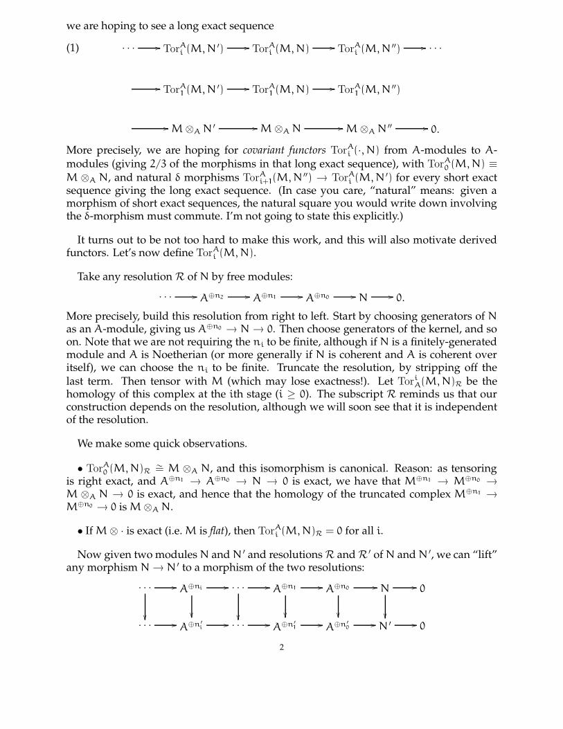
we are hoping to see a long exact sequence

(1) · · · // TorAi (M, N ′) // Tor

Ai (M, N) // Tor

Ai (M, N ′′) // · · ·

// TorA1 (M, N ′) // Tor

A1 (M, N) // Tor

A1 (M, N ′′)

// M ⊗A N ′ // M ⊗A N // M ⊗A N ′′ // 0.

More precisely, we are hoping for covariant functors TorAi (·, N) from A-modules to A-

modules (giving 2/3 of the morphisms in that long exact sequence), with TorA0 (M, N) ≡

M ⊗A N, and natural δ morphisms TorAi+1(M, N ′′) → Tor

Ai (M, N ′) for every short exact

sequence giving the long exact sequence. (In case you care, “natural” means: given amorphism of short exact sequences, the natural square you would write down involvingthe δ-morphism must commute. I’m not going to state this explicitly.)

It turns out to be not too hard to make this work, and this will also motivate derivedfunctors. Let’s now define Tor

Ai (M, N).

Take any resolution R of N by free modules:· · · // A⊕n2 // A⊕n1 // A⊕n0 // N // 0.

More precisely, build this resolution from right to left. Start by choosing generators of N

as an A-module, giving us A⊕n0→ N → 0. Then choose generators of the kernel, and so

on. Note that we are not requiring the ni to be finite, although if N is a finitely-generatedmodule and A is Noetherian (or more generally if N is coherent and A is coherent overitself), we can choose the ni to be finite. Truncate the resolution, by stripping off thelast term. Then tensor with M (which may lose exactness!). Let Tor

iA(M, N)R be the

homology of this complex at the ith stage (i ≥ 0). The subscript R reminds us that ourconstruction depends on the resolution, although we will soon see that it is independentof the resolution.

We make some quick observations.

• TorA0 (M, N)R ∼= M ⊗A N, and this isomorphism is canonical. Reason: as tensoring

is right exact, and A⊕n1→ A⊕n0

→ N → 0 is exact, we have that M⊕n1→ M⊕n0

→

M ⊗A N → 0 is exact, and hence that the homology of the truncated complex M⊕n1→

M⊕n0→ 0 is M ⊗A N.

• If M ⊗ · is exact (i.e. M is flat), then TorAi (M, N)R = 0 for all i.

Now given two modules N and N ′ and resolutions R and R ′ of N and N ′, we can “lift”any morphism N → N ′ to a morphism of the two resolutions:

· · · //

��

A⊕ni //

��

· · · //

��

A⊕n1 //

��

A⊕n0 //

��

N

��

// 0

· · · // A⊕n ′

i// · · · // A⊕n ′

1// A⊕n ′

0// N ′ // 0

2

Here we are using the freeness of A⊗ni : if a1, . . . , aniare generators of A⊗ni , to lift the

map b : A⊗ni→ A⊗n ′

i−1 to c : A⊗ni→ A⊗n ′

i , we arbitrarily lift b(ai) from A⊗n ′

i−1 to A⊗n ′

i ,and declare this to be c(ai).

Denote the choice of lifts by R → R ′. Now truncate both complexes (remove columnN → N ′) and tensor with M. Maps of complexes induce maps of homology, so we havedescribed maps (a priori depending on R → R ′)

TorAi (M, N)R → Tor

Ai (M, N ′)R ′.

We say two maps of complexes f, g : C∗ → C ′∗ are homotopic if there is a sequence of

maps w : Ci → C ′i+1 such that f − g = dw + wd. Two homotopic maps give the same map

on homology. (Exercise: verify this if you haven’t seen this before.)

1.A. CRUCIAL EXERCISE. Show that any two lifts R → R ′ are homotopic.

We now pull these observations together.

(1) We get a covariant functor from TorAi (M, N)R → Tor

Ai (M, N ′)R ′ , independent of

the lift R → R ′.(2) Hence for any two resolutions R andR ′ we get a canonical isomorphism Tor

Ai (M, N)R ∼=

Tor1i (M, N)R ′. Here’s why. Choose lifts R → R ′ and R ′

→ R. The compositionR → R ′

→ R is homotopic to the identity (as it is a lift of the identity map N → N).Thus if fR→R ′ : Tor

Ai (M, N)R → Tor

1i (M, N)R ′ is the map induced by R → R ′, and

similarly fR ′→R is the map induced by R → R ′, then fR ′

→R ◦ fR→R ′ is the identity,and similarly fR→R ′ ◦ fR ′

→R is the identity.(3) Hence the covariant functor doesn’t depend on the resolutions!

Finally:(4) For any short exact sequence we get a long exact sequence of Tor’s (1). Here’s why:given a short exact sequence, choose resolutions of N ′ and N ′′. Then use these to get aresolution for N in the obvious way (see below; the map A⊕(n ′

0→n ′′

0)→ N is the composi-

tion A⊕n ′

0 → N ′→ N along with any lift of An ′′

0 → N ′′ to N) so that we have a short exact

3

sequence of resolutions

0

��

0

��

0

��

· · · // A⊕n ′

1

��

// A⊕n ′

0

��

// N ′

��

// 0

· · · // A⊕(n ′

1+n ′′

1)

��

// A⊕(n ′

0+n ′′

0)

��

// N

��

// 0

· · · // A⊕n ′′

1

��

// A⊕n ′′

0

��

// N ′′

��

// 0

0 0 0

Then truncate (removing the right column 0 → N ′→ N → N ′′

→ 0), tensor with M

(obtaining a short exact sequence of complexes) and take cohomology, yielding a longexact sequence.

We have thus established the foundations of Tor!

Note that if N is a free module, then TorAi (M, N) = 0 for all M and all i > 0, as N has

the trivial resolution 0 → N → N → 0 (it is “its own resolution”).

1.B. EXERCISE. Show that the following are equivalent conditions on an A-module M.

(i) M is flat(ii) Tor

Ai (M, N) = 0 for all i > 0 and all A-modules N,

(iii) TorA1 (M, N) = 0 for all A-modules N.

2. FROM TOR TO DERIVED FUNCTORS IN GENERAL

2.1. Projective resolutions. We used very little about free modules in the above constructionof Tor; in fact we used only that free modules are projective, i.e. those modules M suchthat for any surjection M ′

→ M ′′, it is possible to lift any morphism M → M ′′ to M → M ′.This is summarized in the following diagram.

M

""E

E

E

E

E

E

E

E

exists��

�

�

M ′ // // M ′′

Equivalently, Hom(M, ·) is an exact functor (Hom(M, ·) is always left-exact for any M).More generally, the same idea yields the definition of a projective object in any abeliancategory. Hence (i) we can compute Tor

Ai (M, N) by taking any projective resolution of

N, and (ii) TorAi (M, N) = 0 for any projective A-module N.

4

2.A. INTERESTING EXERCISE: DERIVED FUNCTORS CAN BE COMPUTED USING ACYCLICRESOLUTIONS. Show that you can also compute derived functor cohomology using flatresolutions, i.e. by a resolution

· · · → F2 → F1 → F0 → N → 0

by flat A-modules. Hint: show that you can construct a double complex

...

��

...

��

...

��

...

��

· · · // A⊕n2,1

��

// A⊕n1,1

��

// A⊕n0,1

��

// A⊕n1

��

// 0

· · · // A⊕n2,0

��

// A⊕n1,0

��

// A⊕n0,0

��

// A⊕n0

��

// 0

· · · // F2// F1

// F0// N // 0

where the rows and columns are exact. Do this by constructing the A⊕?? inductively fromthe bottom left. Tensor the double complex with M, to obtain a new double complex.Remove the bottom row, and the right-most nonzero column. Use a spectral sequenceargument to show that (i) the double complex has homology equal to Tor, and (ii) the ho-mology of the double complex agrees with the homology of the free resolution (truncated)tensored with M.

You will notice in the solution to the above exercise that what mattered was that flatmodules had no higher Tor’s (Exercise 1.B). This will later directly generalize to the state-ments that derived functors can be computed with acyclic resolutions (“acyclic” means “nohigher (co)homology”).

2.2. Derived functors of right-exact functors.

The above description was low-tech, but immediately generalizes drastically. All weare using is that M⊗A is a right-exact functor. In general, if F is any right-exact covariantfunctor from the category of A-modules to any abelian category, this construction willdefine a sequence of functors LiF (called left-derived functors of F) such that L0F = F andthe Li’s give a long-exact sequence. We can make this more general still. We say that anabelian category has enough projectives if for any object N there is a surjection onto itfrom a projective object. Then if F is any right-exact functor from an abelian category withenough projectives to any abelian category, then F has left-derived functors.

2.B. UNIMPORTANT EXERCISE. Show that an object P is projective if and only if everyshort exact sequence 0 → A → B → P → 0 splits.

2.C. EXERCISE. The notion of an injective object in an abelian category is dual to thenotion of a projective object. (a) State precisely the definition of an injective object. (b)Define derived functors for (i) covariant left-exact functors (these are called right-derived

5

functors), (ii) contravariant left-exact functors (also called right-derived functors), and(iii) contravariant right-exact functors (these are called left-derived functors), making ex-plicit the necessary assumptions of the category having enough injectives or projectives.

2.3. Notation. If F is a right-exact functor, its (left-)derived functors are denoted LiF (i ≥ 0,with L0F = F). If F is a left-exact functor, its (right-) derived functors are denoted RiF.


6

SPECTRAL SEQUENCES: FRIEND OR FOE?

RAVI VAKIL

Spectral sequences are a powerful book-keeping tool for proving things involving com-plicated commutative diagrams. They were introduced by Leray in the 1940’s at the sametime as he introduced sheaves. They have a reputation for being abstruse and difficult.It has been suggested that the name ‘spectral’ was given because, like spectres, spectralsequences are terrifying, evil, and dangerous. I have heard no one disagree with thisinterpretation, which is perhaps not surprising since I just made it up.

Nonetheless, the goal of this note is to tell you enough that you can use spectral se-quences without hesitation or fear, and why you shouldn’t be frightened when they comeup in a seminar. What is different in this presentation is that we will use spectral sequenceto prove things that you may have already seen, and that you can prove easily in otherways. This will allow you to get some hands-on experience for how to use them. Wewill also see them only in a “special case” of double complexes (which is the versionby far the most often used in algebraic geometry), and not in the general form usuallypresented (filtered complexes, exact couples, etc.). See chapter 5 of Weibel’s marvelousbook for more detailed information if you wish. If you want to become comfortable withspectral sequences, you must try the exercises.

For concreteness, we work in the category vector spaces over a given field. However,everything we say will apply in any abelian category, such as the category ModA of A-modules.

0.1. Double complexes.

A first-quadrant double complex is a collection of vector spaces Ep,q (p, q ∈ Z), whichare zero unless p, q ≥ 0, and “rightward” morphisms d

p,q> : Ep,q

→ Ep,q+1 and “upward”morphisms d

p,q∧

: Ep,q→ Ep+1,q. In the superscript, the first entry denotes the row number,

and the second entry denotes the column number, in keeping with the convention formatrices, but opposite to how the (x, y)-plane is labeled. The subscript is meant to suggestthe direction of the arrows. We will always write these as d> and d∧ and ignore thesuperscripts. We require that d> and d∧ satisfying (a) d2

> = 0, (b) d2∧

= 0, and one morecondition: (c) either d>d∧ = d∧d> (all the squares commute) or d>d∧ + d∧d> = 0 (theyall anticommute). Both come up in nature, and you can switch from one to the other byreplacing d

p,q∧

with dp∧(−1)q. So I’ll assume that all the squares anticommute, but that

you know how to turn the commuting case into this one. (You will see that there is nodifference in the recipe, basically because the image and kernel of a homomorphism f

equal the image and kernel respectively of −f.)

Date: Tuesday, March 12, 2008. Updated version later Tuesday afternoon.

1

Ep+1,qd

p+1,q> // Ep+1,q+1

anticommutes

Ep,q

dp,q

∧

OO

dp,q> // Ep,q+1

dp,q+1∧

OO

There are variations on this definition, where for example the vertical arrows go down-wards, or some different subset of the Ep,q are required to be zero, but I’ll leave thesestraightforward variations to you.

From the double complex we construct a corresponding (single) complex E• with Ek =

⊕iEi,k−i, with d = d> + d∧. In other words, when there is a single superscript k, we mean

a sum of the kth antidiagonal of the double complex. The single complex is somtimescalled the total complex. Note that d2 = (d> + d∧)2 = d2

> + (d>d∧ + d∧d>) + d2∧

= 0, soE• is indeed a complex.

The cohomology of the single complex is sometimes called the hypercohomology ofthe double complex. We will instead use the phrase “cohomology of the double complex”.

Our initial goal will be to find the cohomology of the double complex. You will seelater that we secretly also have other goals.

A spectral sequence is a recipe for computing some information about the cohomologyof the double complex. I won’t yet give the full recipe. Surprisingly, this fragmentary bitof information is sufficent to prove lots of things.

0.2. Approximate Definition. A spectral sequence with rightward orientation is asequence of tables or pages >E

p,q0 , >E

p,q1 , >E

p,q2 , . . . (p, q ∈ Z), where >E

p,q0 = Ep,q, along

with a differential

>dp,qr : >Ep,q

r → >Ep+r,q−r+1

with >dp,qr ◦ >dp,q

r = 0, along with an isomorphism of the cohomology of >dr at >Ep,q (i.e.ker >dp,q

r / im >dp−r,q+r−1r ) with >E

p,qr+1.

The orientation indicates that our 0th differential is the rightward one: d0 = d>. Theleft subscript “>” is usually omitted.

2

The order of the morphisms is best understood visually:(1) •

•

•

•d0

//

d1

OOd2

WW//

/

/

/

/

/

/

/

/

/

/

/

/

d3

ZZ55

5

5

5

5

5

5

5

5

5

5

5

5

5

5

5

5

5

5

5

5

5

5

•

(the morphisms each apply to different pages). Notice that the map always is “degree 1”in the grading of the single complex E•.

The actual definition describes what E•,•r and d•,•

r actually are, in terms of E•,•. We willdescribe d0, d1, and d2 below, and you should for now take on faith that this sequencecontinues in some natural way.

Note that Ep,qr is always a subquotient of the corresponding term on the 0th page E

p,q0 =

Ep,q. In particular, if Ep,q = 0, then Ep,qr = 0 for all r, so Ep,q

r = 0 unless p, q ∈ Z≥0. Notice

also that for any fixed p, q, once r is sufficiently large, Ep,qr+1 is computed from (E•,•

r , dr)

using the complex0

Ep,qr

dp,qr

YY33

3

3

3

3

3

3

3

3

3

3

3

0

dp+r,q−r−1r

YY33

3

3

3

3

3

3

3

3

3

3

3

and thus we have canonical isomorphismsEp,q

r∼= E

p,qr+1

∼= Ep,qr+2

∼= · · ·

We denote this module Ep,q∞

.

We now describe the first few pages of the spectral sequence explicitly. As stated above,the differential d0 on E•,•

0 = E•,• is defined to be d>. The rows are complexes:• // • // •

The 0th page E0: • // • // •

• // • // •

3

and so E1 is just the table of cohomologies of the rows. You should check that thereare now vertical maps d

p,q1 : E

p,q1 → E

p+1,q1 of the row cohomology groups, induced by

d∧, and that these make the columns into complexes. (We have “used up the horizontalmorphisms”, but “the vertical differentials live on”.)

• • •

The 1st page E1: •

OO

•

OO

•

OO

•

OO

•

OO

•

OO

We take cohomology of d1 on E1, giving us a new table, Ep,q2 . It turns out that there

are natural morphisms from each entry to the entry two above and one to the left, andthat the composition of these two is 0. (It is a very worthwhile exercise to work outhow this natural morphism d2 should be defined. Your argument may be reminiscent ofthe connecting homomorphism in the Snake Lemma 0.5 or in the long exact sequence incohomology arising from a short exact sequence of complexes, Exercise 0.D. This is nocoincidence.)

• • •

The 2nd page E2: • • •

• •

VV..

.

.

.

.

.

.

.

.

.

.

.

.

.

•

VV..

.

.

.

.

.

.

.

.

.

.

.

.

.

This is the beginning of a pattern.

Then it is a theorem that there is a filtration of Hk(E•) by Ep,q∞

where p + q = k. (Wecan’t yet state it as an official Theorem because we haven’t precisely defined the pagesand differentials in the spectral sequence.) More precisely, there is a filtration

(2) E0,k∞

�

�E1,k−1∞ // ?

�

�E2,k−2∞ // · · · �

� Ek,0// Hk(E•)

where the quotients are displayed above each inclusion. (I always forget which way thequotients are supposed to go, i.e. whether Ek,0 or E0,k is the subobject. One way of re-membering it is by having some idea of how the result is proved.)

We say that the spectral sequence >E•,•• converges to H•(E•). We often say that >E•,•

2 (orany other page) abuts to H•(E•).

Although the filtration gives only partial information about H•(E•), sometimes one canfind H•(E•) precisely. One example is if all Ei,k−i

∞are zero, or if all but one of them are zero

(e.g. if Ei,k−ir has precisely one non-zero row or column, in which case one says that the

spectral sequence collapses at the rth step, although we will not use this term). Anotherexample is in the category of vector spaces over a field, in which case we can find thedimension of Hk(E•). Also, in lucky circumstances, E2 (or some other small page) alreadyequals E∞.

4

0.A. EXERCISE: INFORMATION FROM THE SECOND PAGE. Show that H0(E•) = E0,0∞

= E0,02

and

0 // E0,12

// H1(E•) // E1,02

d1,02 // E0,2

2// H2(E•).

0.3. The other orientation.

You may have observed that we could as well have done everything in the opposite di-rection, i.e. reversing the roles of horizontal and vertical morphisms. Then the sequencesof arrows giving the spectral sequence would look like this (compare to (1)).

(3) •

•

OO

//

''O

O

O

O

O

O

O

O

O

O

O

O

O

O

%%J

J

J

J

J

J

J

J

J

J

J

J

J

J

J

J

J

J

J

J

J

J

J

J

•

•

•

This spectral sequence is denoted ∧E•,•• (“with the upwards orientation”). Then we would

again get pieces of a filtration of H•(E•) (where we have to be a bit careful with the orderwith which ∧Ep,q

∞corresponds to the subquotients — it in the opposite order to that of (2)

for >Ep,q∞

). Warning: in general there is no isomorphism between >Ep,q∞

and ∧Ep,q∞

.

In fact, this observation that we can start with either the horizontal or vertical mapswas our secret goal all along. Both algorithms compute information about the same thing(H•(E•)), and usually we don’t care about the final answer — we often care about theanswer we get in one way, and we get at it by doing the spectral sequence in the otherway.

0.4. Examples.

We’re now ready to see how this is useful. The moral of these examples is the following.In the past, you may have proved various facts involving various sorts of diagrams, whichinvolved chasing elements around. Now, you’ll just plug them into a spectral sequence,and let the spectral sequence machinery do your chasing for you.

0.5. Example: Proving the Snake Lemma. Consider the diagram

0 // D // E // F // 0

0 // A //

α

OO

B //

β

OO

C

γ

OO

// 0

5

where the rows are exact and the squares commute. (Normally the Snake Lemma is de-scribed with the vertical arrows pointing downwards, but I want to fit this into my spec-tral sequence conventions.) We wish to show that there is an exact sequence

(4) 0 → ker α → ker β → ker γ → im α → im β → im γ → 0.

We plug this into our spectral sequence machinery. We first compute the cohomologyusing the rightwards orientation, i.e. using the order (1). Then because the rows are exact,E

p,q1 = 0, so the spectral sequence has already converged: Ep,q

∞= 0.

We next compute this “0” in another way, by computing the spectral sequence usingthe upwards orientation. Then ∧E•,•

1 (with its differentials) is:

0 // im α // im β // im γ // 0

0 // ker α // ker β // ker γ // 0.

Then ∧E•,•2 is of the form:

0

''N

N

N

N

N

N

N

N

N

N

N

N

N

N 0

''N

N

N

N

N

N

N

N

N

N

N

N

N

N

N

0

''N

N

N

N

N

N

N

N

N

N

N

N

N

N

N ??

''N

N

N

N

N

N

N

N

N

N

N

N

N

N ?

''N

N

N

N

N

N

N

N

N

N

N

N

N

N

N ? 0

0 ? ?

''N

N

N

N

N

N

N

N

N

N

N

N

N

N

N ??

''N

N

N

N

N

N

N

N

N

N

N

N

N

N 0

0 0

We see that after ∧E2, all the terms will stabilize except for the double-question-marks —all maps to and from the single question marks are to and from 0-entries. And after ∧E3,even these two double-quesion-mark terms will stabilize. But in the end our complexmust be the 0 complex. This means that in ∧E2, all the entries must be zero, except forthe two double-question-marks, and these two must be the isormorphic. This means that0 → ker α → ker β → ker γ and im α → im β → im γ → 0 are both exact (that comes fromthe vanishing of the single-question-marks), and

coker(ker β → ker γ) ∼= ker(imα → im β)

is an isomorphism (that comes from the equality of the double-question-marks). Takentogether, we have proved the exactness of (4), and hence the Snake Lemma!

Spectral sequences make it easy to see how to generalize results further. For example,if A → B is no longer assumed to be injective, how would the conclusion change?

6

0.6. Example: the Five Lemma. Suppose

(5) F // G // H // I // J

A //

α

OO

B //

β

OO

C

γ

OO

// D //

δ

OO

E

ε

OO

where the rows are exact and the squares commute.

Suppose α, β, δ, ε are isomorphisms. We’ll show that γ is an isomorphism.

We first compute the cohomology of the total complex using the rightwards orientation(1). We choose this because we see that we will get lots of zeros. Then >E•,•

1 looks like this:

? 0 0 0 ?

?

OO

0

OO

0

OO

0

OO

?

OO

Then >E2 looks similar, and the sequence will converge by E2, as we will never get anyarrows between two non-zero entries in a table thereafter. We can’t conclude that thecohomology of the total complex vanishes, but we can note that it vanishes in all butfour degrees — and most important, it vanishes in the two degrees corresponding to theentries C and H (the source and target of γ).

We next compute this using the upwards orientation (3). Then ∧E1 looks like this:

0 // 0 // ? // 0 // 0

0 // 0 // ? // 0 // 0

and the spectral sequence converges at this step. We wish to show that those two questionmarks are zero. But they are precisely the cohomology groups of the total complex thatwe just showed were zero — so we’re done!

The best way to become comfortable with this sort of argument is to try it out yourselfseveral times, and realize that it really is easy. So you should do the following exercises!

0.B. EXERCISE: THE SUBTLE FIVE LEMMA. By looking at the spectral sequence proofof the Five Lemma above, prove a subtler version of the Five Lemma, where one of theisomorphisms can instead just be required to be an injection, and another can instead justbe required to be a surjection. (I am deliberately not telling you which ones, so you cansee how the spectral sequence is telling you how to improve the result.)

0.C. EXERCISE. If β and δ (in (5)) are injective, and α is surjective, show that γ is injective.State the dual statement (whose proof is of course essentially the same).

0.D. EXERCISE. Use spectral sequences to show that a short exact sequence of complexesgives a long exact sequence in cohomology.

7

0.E. EXERCISE (THE MAPPING CONE). Suppose µ : A•→ B• is a morphism of complexes.

Suppose C• is the single complex associated to the double complex A•→ B•. (C• is called

the mapping cone of µ.) Show that there is a long exact sequence of complexes:

· · · → Hi−1(C•) → Hi(A•) → Hi(B•) → Hi(C•) → Hi+1(A•) → · · · .

(There is a slight notational ambiguity here; depending on how you index your doublecomplex, your long exact sequence might look slightly different.) In particular, we willuse the fact that µ induces an isomorphism on cohomology if and only if the mappingcone is exact.

You are now ready to go out into the world and use spectral sequences to your heart’scontent!

0.7. ?? Complete definition of the spectral sequence, and proof.

You should most definitely not read this section any time soon after reading the intro-duction to spectral sequences above. Instead, flip quickly through it to convince yourselfthat nothing fancy is involved.

We consider the rightwards orientation. The upwards orientation is of course a trivialvariation of this.

0.8. Goals. We wish to describe the pages and differentials of the spectral sequenceexplicitly, and prove that they behave the way we said they did. More precisely, we wishto:

(a) describe Ep,qr ,

(b) verify that Hk(E•) is filtered by Ep,k−p∞

as in (2),(c) describe dr and verify that d2

r = 0, and(d) verify that E

p,qr+1 is given by cohomology using dr.

Before tacking these goals, you can impress your friends by giving this short descrip-tion of the pages and differentials of the spectral sequence. We say that an element of E•,•

is a (p, q)-strip if it is an element of ⊕l≥0Ep+l,q−l (see Fig. 1). Its non-zero entries lie on a

semi-infinite antidiagonal starting with position (p, q). We say that the (p, q)-entry (theprojection to Ep,q) is the leading term of the (p, q)-strip. Let Sp,q ⊂ E•,• be the submoduleof all the (p, q)-strips. Clearly Sp,q ⊂ Ep+q, and S0,k = Ek.

Note that the differential d = d∧ +d> sends a (p, q)-strip x to a (p, q+ 1)-strip dx. If dx

is furthermore a (p + r, q + r + 1)-strip (r ∈ Z≥0), we say that x is an r-closed (p, q)-strip.

We denote the set of such Sp,qr (so for example S

p,q0 = Sp,q, and S0,k

0 = Ek). An element of

8

. . . 0 0 0 0

0 ∗p+2,q−2 0 0 0

0 0 ∗p+1,q−1 0 0

0 0 0 ∗p,q 0

0 0 0 0 0p−1,q+1

FIGURE 1. A (p, q)-strip (in Sp,q ⊂ Ep+q). Clearly S0,k = Ek.

Sp,qr may be depicted as:

. . . // ?

∗p+2,q−2

OO

// 0

∗p+1,q−1

OO

// 0

∗p,q //

OO

0

0.9. Preliminary definition of Ep,qr . We are now ready to give a first definition of Ep,q

r ,which by construction should be a subquotient of Ep,q = E

p,q0 . We describe it as such by

describing two submodules Yp,qr ⊂ Xp,q

r ⊂ Ep,q, and defining Ep,qr = Xp,q

r /Yp,qr . Let Xp,q

r

be those elements of Ep,q that are the leading terms of r-closed (p, q)-strips. Note thatby definition, d sends (r − 1)-closed Sp−(r−1),q+(r−1)−1-strips to (p, q)-strips. Let Yp,q

r be theleading ((p, q))-terms of the differential d of (r−1)-closed (p−(r−1), q+(r−1)−1)-strips(where the differential is considered as a (p, q)-strip).

We next give the definition of the differential dr of such an element x ∈ Xp,qr . We take

any r-closed (p, q)-strip with leading term x. Its differential d is a (p + r, q − r + 1)-strip,and we take its leading term. The choice of the r-closed (p, q)-strip means that this is not awell-defined element of Ep,q. But it is well-defined modulo the (r−1)-closed (p+1, r+1)-strips, and hence gives a map Ep,q

r → Ep+r,q−r+1r .

This definition is fairly short, but not much fun to work with, so we will forget it, andinstead dive into a snakes’ nest of subscripts and superscripts.

9

We begin with making some quick but important observations about (p, q)-strips.

0.F. EXERCISE. Verify the following.

(a) Sp,q = Sp+1,q−1 ⊕ Ep,q.(b) (Any closed (p, q)-strip is r-closed for all r.) Any element x of Sp,q = S

p,q0 that is a

cycle (i.e. dx = 0) is automatically in Sp,qr for all r. For example, this holds when x

is a boundary (i.e. of the form dy).(c) Show that for fixed p, q,

Sp,q0 ⊃ S

p,q1 ⊃ · · · ⊃ Sp,q

r ⊃ · · ·

stabilizes for r � 0 (i.e. Sp,qr = S

p,qr+1 = · · · ). Denote the stabilized module Sp,q

∞.

Show Sp,q∞

is the set of closed (p, q)-strips (those (p, q)-strips annihilated by d, i.e.the cycles). In particular, S0,k

r is the set of cycles in Ek.

0.10. Defining Ep,qr .

Define Xp,qr := Sp,q

r /Sp+1,q−1r−1 and Y := dS

p−(r−1),q+(r−1)−1

r−1 /Sp+1,q−1r−1 .

Then Yp,qr ⊂ Xp,q

r by Exercise 0.F(b). We define

(6) Ep,qr =

Xp,qr

Yp,qr

=Sp,q

r

dSp−(r−1),q+(r−1)−1

r−1 + Sp+1,q−1r−1

We have completed Goal 0.8(a).

You are welcome to verify that these definitions of Xp,qr and Yp,q

r and hence Ep,qr agree

with the earlier ones of §0.9 (and in particular Xp,qr and Yp,q

r are both submodules of Ep,q),but we won’t need this fact.

0.G. EXERCISE: Ep,k−p∞

GIVES SUBQUOTIENTS OF Hk(E•). By Exercise 0.F(c), Ep,qr stabilizes

as r → ∞. For r � 0, interpret Sp,qr /dS

p−(r−1),q+(r−1)−1

r−1 as the cycles in Sp,q∞

⊂ Ep+q modulothose boundary elements of dEp+q−1 contained in Sp,q

∞. Finally, show that Hk(E•) is indeed

filtered as described in (2).

We have completed Goal 0.8(b).

0.11. Definition of dr.

We shall see that the map dr : Ep,qr → Ep+r,q−r+1 is just induced by our differential d.

Notice that d sends r-closed (p, q)-strips Sp,qr to (p + r, q − r + 1)-strips Sp+r,q−r+1, by the

definition “r-closed”. By Exercise 0.F(b), the image lies in Sp+r,q−r+1r .

0.H. EXERCISE. Verify that d sends

dSp−(r−1),q+(r−1)−1

r−1 + Sp+1,q−1r−1 → dS

(p+r)−(r−1),(q−r+1)+(r−1)−1

r−1 + S(p+r)+1,(q−r+1)−1

r−1 .

10

(The first term on the left goes to 0 from d2 = 0, and the second term on the left goes tothe first term on the right.)

Thus we may define

dr : Ep,qr =

Sp,qr

dSp−(r−1),q+(r−1)−1

r−1 + Sp+1,q−1r−1

→

Sp+r,q−r+1r

dSp+1,q−1r−1 + S

p+r+1,q−rr−1

= Ep+r,q−r+1r

and clearly d2r = 0 (as we may interpret it as taking an element of Sp,q

r and applying d

twice).

We have accomplished Goal 0.8(c).

0.12. Verifying that the cohomology of dr at Ep,qr is E

p,qr+1. We are left with the unpleasant job

of verifying that the cohomology of

(7) Sp−r,q+r−1r

dSp−2r+1,q−3r−1

+Sp−r+1,q+r−2r−1

dr // Sp,qr

dSp−r+1,q+r−2r−1

+Sp+1,q−1r−1

dr // Sp+r,q−r+1r

dSp+1,q−1r−1

+Sp+r+1,q−rr−1

is naturally identified withS

p,qr+1

dSp−r,q+r−1r + S

p+1,q−1r

and this will conclude our final Goal 0.8(d).

Let’s begin by understanding the kernel of the right map of (7). Suppose a ∈ Sp,qr is

mapped to 0. This means that da = db+c, where b ∈ Sp+1,q−1r−1 . If u = a−b, then u ∈ Sp,q,

while du = c ∈ Sp+r+1,q−rr−1 ⊂ Sp+r+1,q−r, from which u is r-closed, i.e. u ∈ S

p,qr+1. Hence

a = b + u + x where dx = 0, from which a − x = b + c ∈ Sp+1,q−1r−1 + S

p,qr+1. However,

x ∈ Sp,q, so x ∈ Sp,qr+1 by Exercise 0.F(b). Thus a ∈ S

p+1,q−1r−1 + S

p,qr+1. Conversely, any

a ∈ Sp+1,q−1r−1 + S

p,qr+1 satisfies

da ∈ dSp+r,q−r+1r−1 + dS

p,qr+1 ⊂ dS

p+r,q−r+1r−1 + S

p+r+1,q−rr−1

(using dSp,qr+1 ⊂ S

p+r+1,q−r0 and Exercise 0.F(b)) so any such a is indeed in the kernel of

Sp,qr →

Sp+r,q−r+1r

dSp+1,q−1r−1 + S

p+r+1,q−rr−1

.

Hence the kernel of the right map of (7) is

ker =S

p+1,q−1r−1 + S

p,qr+1

dSp−r+1,q+r−2r−1 + S

p+1,q−1r−1

.

Next, the image of the left map of (7) is immediately

im =dSp−r,q+r−1

r + dSp−r+1,q+r−2r−1 + S

p+1,q−1r−1


p+1,q−1r−1

=dSp−r,q+r−1

r + Sp+1,q−1r−1


p+1,q−1r−1

11

(as Sp−r,q−r+1r contains S

p−r+1,q+r−1r−1 ).

Thus the cohomology of (7) is

ker / im =S

p+1,q−1r−1 + S

p,qr+1

dSp−r,q+r−1r + S

p+1,q−1r−1

=S

p,qr+1

Sp,qr+1 ∩ (dS

p−r,q+r−1r + S

p+1,q−1r−1 )

where the equality on the right uses the fact that dSp−r,q+r+1r ⊂ S

p,qr+1 and an isomorphism

theorem. We thus must showSp,q

r+1 ∩ (dSp−r,q+r−1r + Sp+1,q−1

r−1 ) = dSp−r,q+r−1r + Sp+1,q−1

r .

However,S

p,qr+1 ∩ (dSp−r,q+r−1

r + Sp+1,q−1r−1 ) = dSp−r,q+r−1

r + Sp,qr+1 ∩ S

p+1,q−1r−1

and Sp,qr+1 ∩ S

p+1,q−1r−1 consists of (p, q)-strips whose differential vanishes up to row p + r,

from which Sp,qr+1 ∩ S

p+1,q−1r−1 = Sp,q

r as desired.

This completes the explanation of how spectral sequences work for a first-quadrantdouble complex. The argument applies without significant change to more general situa-tions, including filtered complexes.


12

FOUNDATIONS OF ALGEBRAIC GEOMETRY CLASS...

Documents

Transcript of FOUNDATIONS OF ALGEBRAIC GEOMETRY CLASS...