using me 2 interpreting profiles using me 2 interpreting profiles.
ROBERT J. SHILLER JOHN Y. CAMPBELL KERMIT L. SCHOENHOLTZ Yale University
Forward Rates and Future Policy: Interpreting the Term Structure
of Interest Rates
INTEREST RATES of all maturities have tended to increase in the past few years when the level of the MI measure of the money stock announced on Fridays has been unexpectedly large. Conversely, interest rates have tended to fall when the announcement has been surprisingly small. Even very long-term interest rates, such as thirty-year government bond yields, respond to the money surprises. The response of short- and long- term interest rates has been sufficiently dramatic to attract considerable attention from market analysts and academic economists. '
We acknowledge helpful discussions with Dale Ballou, Paul Boltz, Carlos F. Diaz- Alejandro, Robert L. Hetzel, Kenneth Kopecky, William C. Melton, William D. Nordhaus, V. Vance Roley, Steve Ross, and participants in seminars at Yale, the University of Pennsylvania, and the National Bureau of Economic Research. We also thank Data Resources, Inc., Salomon Brothers, Money Market Services, Inc., and the Federal Reserve Board for providing data. This research was supported by the National Science Foundation under grant SES-8105837.
1. See Bradford Cornell, "Money Supply Announcements and Interest Rates: Another View," Journal of Business, vol. 56 (January 1983), pp. 1-23; Charles Engel and Jeffrey A. Frankel, "Why Money Announcements Move Interest Rates: An Answer from the Foreign Exchange Market, " Working Paper (University of California at Berkeley, January 1982); Donald A. Nichols, John H. Small, and Charles E. Webster, "Why Interest Rates Rise When An Unexpectedly Large Money Stock Is Announced," American Economic Review, vol. 73 (June 1983), pp. 383-88; V. Vance Roley, "The Response of Short-Term Interest Rates to Weekly Money Announcements, " Working Paper 1001 (National Bureau of Economic Research, October 1982); and Thomas Urich and Paul Wachtel, "The Effects of Inflation and Money Supply Announcements on Interest Rates" (New York University, Graduate School of Business, August 1982).
173

174 Brookings Papers on Economic Activity, 1:1983
In the same period there has been a general perception that long-term interest rates have been "too high." What seems to be meant by this is that long-term rates are unusually high given the recent behavior of short-term interest rates (and other variables, such as inflation, which may affect long-term rates). We confirm that long-term rates in the past two years have been substantially higher than those predicted using a term-structure equation like those commonly found in macroeconometric models.2
We are concerned in this paper with basic methods of interpreting these and similar term-structure phenomena. Our purpose is to deter- mine whether a simple theory, without major modification, can be used to explain the observed behavior of longer-term yields. The most important of such "simple theories" is the expectations theory of the term structure, which confines attention to the forecasting process for short-term interest rates.
The expectations model has been used as a workhorse for many policy discussions. While practitioners have incorporated risk factors in the form of a constant or even a slowly moving risk premium, they have not focused on changes in risk as the primary interpretation of interest rate phenomena. Thus changes in the shape of the term structure are still understood to reflect a changed outlook for future interest rates relative to current rates. According to the model, even though policy authorities can accurately control short-term rates, the authorities affect long-term rates only insofar as they influence a long weighted average of present and expected future short-term rates.
The simple expectations theory, in combination with the hypothesis of rational expectations, has been rejected many times in careful econ- ometric studies.3 But the theory seems to reappear perennially in policy
2. See table 2. The equation is similar to the one estimated in Modigliani and Shiller, which has since been used as a structural equation in the MIT-Pennsylvania-Social Science Research Council (MPS) model of the United States economy. See Franco Modigliani and Robert J. Shiller, "Inflation, Rational Expectations and the Term Structure of Interest Rates," Economica, vol. 40 (February 1973), pp. 12-43. Their equation was motivated by the idea that distributed lags on short-term interest rates and inflation rates might represent expectations of the long-run path of future interest rates.
3. For example, Lars Peter Hansen and Thomas J. Sargent, "Exact Linear Rational Expectations Models: Specification and Estimation," Staff Report 71 (Federal Reserve Bank of Minneapolis, September 1981); Richard Roll, The Behavior of Interest Rates (Basic Books, 1970); Thomas J. Sargent, "A Note on Maximum Likelihood Estimation of the Rational Expectations Model of the Term Structure, " Journal of Monetary Economics,

R. J. Shiller, J. Y. Campbell, and K. L. Schoenholtz 175
discussions as if nothing had happened to it. It is uncanny how resistant superficially appealing theories in economics are to contrary evidence. We are reminded of the Tom and Jerry cartoons that precede feature films at movie theatres. The villain, Tom the cat, may be buried under a ton of boulders, blasted through a brick wall (leaving a cat-shaped hole), or flattened by a steamroller. Yet seconds later he is up again plotting his evil deeds.
Apparently those who are interested in practical policy discussions believe there is an element of truth to the theory that survives all the attacks. Our major objective here is to help the reader formulate an opinion about the usefulness of the simple expectations model. For this purpose we compare the model with an alternative, which we call the "tail-wags-dog" theory. This says that long-term interest rates may overreact to information relevant only to short-term rates.4
In the following section we develop a linear analytical framework in which the simple expectations model of the term structure can be embedded. Linear approximations have long played a pivotal role in studies of the term structure. Nonetheless, such linearized models have never been given a complete and unified development. We take the opportunity here to fill this void by deriving new general linearized expressions for forward rates and holding-period yields. We examine the accuracy of the linearized expressions for the recent period of higher interest rate volatility. Since the linearization effectively assumes that "duration" (defined below) is constant, we also look at the effects of changing duration on the predictive power of a term-structure equation.
We go on to evaluate the linearized expectations model as a descrip- tion of the observed behavior of interest rates and attempt to improve
vol 5 (January 1979), pp. 133-43, and "Rational Expectations and the Term Structure of Interest Rates," Journal of Money, Credit and Banking, vol. 4 (February 1972), pp. 74- 97; and Robert J. Shiller, "The Volatility of Long-Term Interest Rates and Expectations Models of the Term Structure," Journal of Political Economy, vol. 87 (December 1979), pp. 1190-1219.
4. Such a theory has been proposed in Amos Tversky and Daniel Kahneman, "Judgment under Uncertainty: Heuristics and Biases," Science, vol. 185 (September 1974), pp. 1124-31. In summarizing experiments by psychologists, Tversky and Kahneman stated that subjects showed "insensitivity to reliability of the evidence" and "unwarranted confidence" in their predictions. Predictions were made based on "representativeness" or similarity, with little regard for statistical evidence. The authors thought the experiments suggested that "even when predictability is nil," investors would react to "information [seemingly] relevant to profit."

176 Brookings Papers on Economic Activity, 1:1983
on this model by taking account of time-varying risk premiums. Finally, we use the linearized expectations model to interpret the effects of money-stock announcements on long-term bond rates. The linearized model enables us to specify more accurately than has been done before how the effect of money surprises is distributed across forward rates at various horizons and maturities. In addition, the model allows us to ask whether the response of forward rates has been appropriate or whether the market has over- or underreacted to the announcements. Thus we can compare the simple expectations theory with a model of the tail- wags-dog variety in which long-term rates overreact to money announce- ments.
A Linearized Model of the Term Structure of Interest Rates
The basic notion that long-term interest rates are related to expecta- tions of future short-term interest rates has presented model builders with some technical difficulties. We outline here a way of dealing with these difficulties that has the advantages of simplicity, generality, time consistency, and direct applicability to familiar data. The approach, which is a generalization of earlier work, consists of linearized approxi- mate expressions for holding-period yields and forward rates and a model that relates these linearized expressions.' The approach is intended to be the simplest possible general formalization of the various intuitive ideas we regularly use to interpret interest rate data.
Expectations theories of the term structure of interest rates have several basic forms. In one form, long-term interest rates are represented as an average of expected future short-term interest rates. In another, forward rates equal the expectations of the corresponding future interest rates. Forward rates, defined formally below, are the future interest rates implicit in the term structure on a given date. In yet another form, expected short-term holding period yields of long-term bonds equal today's short-term interest rate. The holding-period yield, also defined formally below, is the total return (coupon and capital gain) to buying a long-term bond and then selling at the end of the holding period. The
5. For earlier work see Shiller, "The Volatility of Long-Term Interest Rates," and "Alternative Tests of Rational Expectations Models: The Case of the Term Structure," Journal of Econometrics, vol. 16 (May 1981), pp. 71-87.

R. J. Shiller, J. Y. Campbell, and K. L. Schoenholtz 177
technical problem that has confronted model builders is that, if mathe- matical expectations are taken to represent market expectations, so long as there is uncertainty about future interest rates these models contradict each other. Moreover, none of the models is time consistent-that is, independent of the time period chosen for analysis. This problem, which has to do with "Jensen's inequality," is described by Cox, Ingersoll, and Ross.6 Our approach approximates all the models by one simple time-consistent model.
Our approach here is more practically oriented than that of most theorists who have considered the modeling difficulties. We want our model to apply to yield data as it is conventionally reported rather than to the returns on the "pure discount" bonds that are analyzed by theorists. Actual bonds with maturities beyond one year almost always carry coupons that, for longer maturities, account for most of the value of the bond. The yields of these bonds cannot be compared with the pure discount forward rates computed by McCulloch and others.7
To understand the importance of coupons, one should consider our first version of the expectations model, which sets the long-term rate as an average of future short-term rates. The standard linearized expecta- tions model for discount bonds expresses the yield on an i-period discount bond as an unweighted average of expected future yields on i one-period discount bonds. This model can be described as having a "flat" weighting scheme. The model we outline below for coupon bonds expresses the yield on an i-period coupon bond as a weighted average of expected future one-period rates, with rates further in the future given less weight. The reason for this declining weighting scheme is that part of the value of a coupon bond is derived from coupon payments that will be made in the near future. The coupon bond can be considered as a package of discount bonds, only one of which has the full maturity of the coupon bond.
Our model is written
(1) R,i) = E W(k)EtR MO k=O
6. John Cox, Jonathan E. Ingersoll, and Stephen A. Ross, "A Re-examination of Traditional Hypotheses about the Term Structure of Interest Rates," Journal of Finance, vol. 36 (September 1981), pp. 769-99.
7. J. Huston McCulloch, "Measuring the Term Structure of Interest Rates," Journal of Business, vol. 44 (January 1971), pp. 19-31.
178 Brookings Papers on Economic Activity, 1:1983
where W(k) = gk(l -g)I(1 - gi), 0 < g < 1. Here, Rfi) is the yield to maturity on an i-period bond at time t; Et denotes mathematical expec- tation conditional on publicly available information at time t; W(k) (k =
0,.. ., i - 1) are weights; and g is a constant discount factor.8 We write the discount rate associated with it as R; then g = 1/(1 + R). For expositional simplicity, we have left out any risk premium, although we modify this equation for empirical work by adding to the right-hand side a risk-premium term, Vi, which depends only on i and which is constant through time.9 With this simplification the i-period rate is a weighted average of expected one-period rates. As described intuitively above, the weights decline monotonically in k and sum to 1.0 [W(O) + W(1) + * + W(i - 1) = 1]. The weighting structure is of the truncated exponential or truncated Koyck variety. For large k (very long-term bonds) the truncation is so far in the future that we can disregard it, and for perpetuities (i = infinity), there is no truncation.
Equation 1 can most easily be understood by use of Macaulay's concept of duration, which is intended as a better measure than the time until maturity of how "long" a bond is.10 The duration of an i-period bond, which pays a coupon each period, with yield to maturity R is defined by
Di= (gci + 2g2c, + * + igic, + igi)1(gc, + g2c, + * + gic, + gi),
where g = 1/(1 + R), ci is the coupon rate of the bond (as a fraction of the principal repaid at maturity), and the denominator is the price of the bond as a fraction of par. Thus the duration of a pure discount bond is its time until maturity but the duration of a coupon bond is less than its time to maturity, reflecting the coupon payments that are made earlier. The higher the level of interest rate for a given maturity i the more the future is discounted and thus the shorter is the duration. We speak here
8. As in Shiller, "The Volatility of Long-Term Interest Rates," and "Alternative Tests of Rational Expectations Models." In the expressions in the text, interest rate is quoted as a rate per period, not percent. Thus, for example, if the time period is monthly and the one-year Treasury bill rate is 6 percent, then RF'2) = 0.005. In the tables, however, rates are percent per year. In all expressions parentheses are used to distinguish superscripts from exponents.
9. The constant risk premium is from Hicks. See J. R. Hicks, Value and Capital (Oxford: Clarendon Press, 1939).
10. Frederick R. Macaulay, Some Theoretical Problems Suggested by the Movements of Interest Rates, Bond Yields, and Stock Prices in the United States Since 1856 (National Bureau of Economic Research, 1938).

R. J. Shiller, J. Y. Campbell, and K. L. Schoenholtz 179
of the duration of an i-period bond as that of a par bond of maturity i- that is, a bond whose coupon rate, ci, is R. Then from Macaulay's formula with ci = R we have
(2) Di = (1 - gi)l(l - g) O c i.
It follows that the model in equation 1 makes the i-period yield, R(i)t equal to the present value, discounted by R, of future one-period rates over the maturity of the bond divided by the duration Di. 1I Alternatively, equation 1 may be described as setting the i-period rate equal to a duration-weighted average of expected future interest rates of any maturities that cover the period from t to t + i.
The above model is a good approximation to the various expectations models of the term structure if interest rates are not so variable that nonlinearities become important. That is, we suppose RW lies in the vicinity of R for all i and t and that the bonds carry coupons in periods t + 1, t + 2, . . ., t + i at a rate (coupon over principal), ci, which is in the vicinity of R. We denote aj-period holding yield for an i-period bond (i > J) as Hfi-J). This is the yield (expressed as a rate per period) from buying an i period bond at time t and selling it at time t + j when the bond has become an i - j period bond. The holding-period yield is computed as the yield to maturity of an asset for which one pays the price of an i-period bond at time t, receives the coupons of the i-period bond, and is finally paid the principal at time t + j (the principal being the price of the bond at time t + j). The holding-period yield depends, therefore, on ROl), RKi+J),P and the coupon on the bond. However, if the implicit expression for Hfi-') is linearized around R for all arguments of the expression-in other words, if we take a Taylor expansion of Hti j) in terms of R?), RKi)JJA, and ci around R truncated after the linear term-we obtain a simple approximate holding period yield,
=DiR) - (Di - Dj)RyiVy) (3) h~~J) = 0 <j
where Di and Dj are the i- and j-period durations given by equation 2. Note that the coupon rate drops out of the expression altogether. In the
11. The mean of the distribution W(k) defined in equation 1 is g/(l - g) - ig/(l - gi). For large i this mean is approximately equal to Di - 1.0. The difference of 1.0 arises because the summation in equation 1 is from zero to i - 1 rather than from 1 to i. For small i the mean is approximately (Di - 1)/2.

180 Brookings Papers on Economic Activity, 1:1983
implicit formula for holding-period yields the coupon effects are of second order. Also note that equation 3 is homogeneous of degree 1 in R't) and RKi+-J), that is, the constant term drops out of the expression. This expression generalizes those that have been obtained in earlier work. When the holding period is one period long (j = 1), the expression reduces by substitution of equation 2 into 3 to that in Shiller.12 As R approaches zero the bonds become discount bonds, Di approaches j, and we obtain
- i - (j) R (i hfi i) = i Ryi) - i j t tJ
The m-period forward rate applying to period t + n is computed from the term structure of interest rates at time t. If we can both borrow and lend at the rates given in the term structure, it is possible to arrange a portfolio that guarantees for us a price of a bond at time t + n maturing at time t + m + n. The procedure is to buy at time t an m + n period bond and to issue bonds of maturities 1, 2, 3, ... , n so that the total value of the portfolio at time t is zero, and so that the value of the stream of payments on issued bonds exactly equals the coupon received on the m + n period bond over all intervening periods, t + 1, t + 2, ... t + n - 1. The net effect, then, will be to lock in a contract to lend at time t + n, receive coupons from t + n + 1 until t + m + n, and be paid back att + m + n.
The yield to maturity on this m-period loan will be called the n-period ahead, m-period forward rate, Fn, m). This forward rate can be computed from R(m+n) and R(1") as well as all other rates, R , . . ., R("- 1), and coupons, cl, c2, . . ., cn,, cn, C,i+m, of the various bonds. If, however, one linearizes the complicated implicit expression for the forward rate around R for all the arguments, a simple linearized approximation, f nm) to the forward rate, F;n, m), results in
(4) n,rn) Dm + -D 0 < m, 0 n,
D7n + 11 Dn
where Dm+n and Dn are durations of bonds maturing in m + n periods and n periods, as given by equation 2. This expression depends only on Rftm +n) and Rin), and not on Ri 1) Ri2) , . . ., 9Ri11- 1) , nor on cl, C2, . . ., Cn - ,,
12. Shiller, "The Volatility of Long-Term Interest Rates."

R. J. Shiller, J. Y. Campbell, and K. L. Schoenholtz 181
Cn cn + m. The effect of these yields and coupons is again of second order and drops out of a linearization. Note also that when m = 1, so that the forward rate is a one-period rate, by using equation 2 this expression reduces to that in Shiller.13 As R approaches zero, the bonds become discount bonds, Dm + n approaches m + n, D,, approaches n, and we obtain
f(,nr) (m + n)R0't'l+) - nRi'I 0 < m, 0 ? n, m
which for m = 1 is the conventional linear approximation. 14
The model in equation 1 then implies
(5) Ethfti = R,j O <; < i
(6) f(n m) = EtR(%), 0 < m, 0 ? n.
Thus the expected linearized holding-period yields on all bonds for all holding intervals are equal to the corresponding spot rates; and linearized forward rates for all future time periods and all maturities equal the corresponding expected spot rates. Moreover, either equation 5 or 6 implies equation 1-that is, subject to the linearizations of forward rates and holding-period yields, all versions of the expectations theory of the term structure can be reconciled.
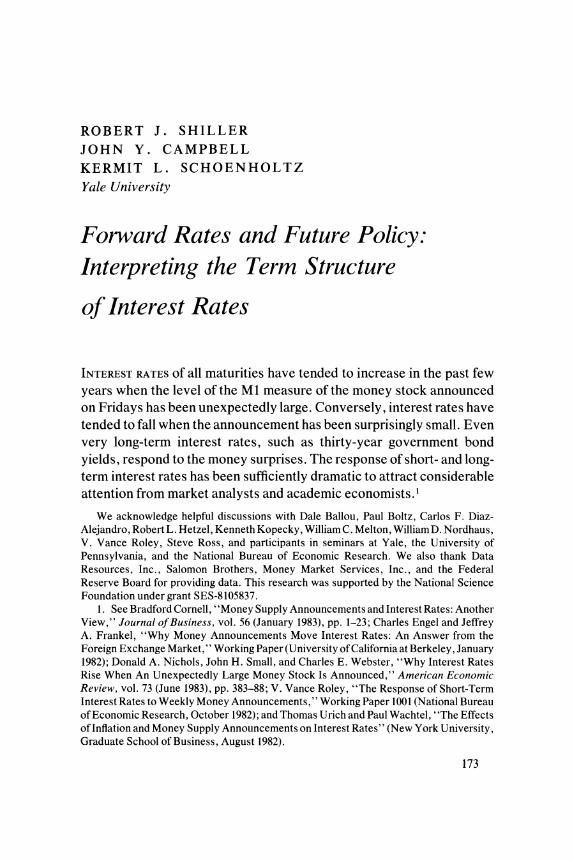
Of course, knowing the quality of the linear approximation is important in judging how well the models have been unified by the linearization. The recent increased variability of interest rates has slightly diminished the accuracy of the linearization. Table 1 shows some data on the quality of approximation over the recent period of volatile interest rates. The point of linearization is generally the mean level of interest rates over the sample period, but in rows 4 and 6 it is varied to the minimum and maximum of the three-month Treasury bill rate over the sample. 15 This change has little effect on the one-year ahead, one-year forward rate or
13. Shiller, "Alternative Tests of Rational Expectations Models." 14. For example, see Roll, The Behavior of Interest Rates. 15. It might be thought desirable to linearize around the current level of the long-term
interest rate at each moment of time. This would produce closer approximations to true holding-period yields or forward rates. But such an approach is not compatible with a linear time-consistent expectations model of the term structure. Therefore we work with a time-invariant point of linearization throughout this paper, although the point chosen does depend on the particular sample period.
0
a- a- q CA o mo aN N ?? o8t n ,- k c
vC
k ) - -) N o ) " N t b o "C
0 -: 0i 0 00 00 O - l sl -l
0
Cu~~~~~~~~~~~~~~~~~~~~~~
t~~~~~ I" I0 r
0
U ? vC~~~~~~~~~~~~~~~~~ ~~~~~ 2
.o
00 l- - 0 V) - o o 0 E X > N v ~~~oo oo oo oo oo oo oo Ntsou
3~~~~~~~~~~~~~~~~~~~~~~~~~~~~ -s
00 00 00 00 0000\00
O~~~~~C ON ONv ON v B ^ O
Cu~~~~~~~~~~~~~~~~~~~~~~~~~~~~~~~~~~~~~~~~~~~~C C o t
O 4 <u)t ? ? 000 00 00 00 1 00 00 " 00 00 X 00 00 00 "C 0
o i > '< * t) t1t 1 t t l ~ )~l ~l l3u ~~00 00 (- 00 cc cc m0 w
N I t- ,.,- <s _e se s
su ~~ . . . . . . . . .oo . u . ov . ..
z > (t O;( (
o sv Q Q~O ON ON ON ON-<
-~~~~~~~~~~~~~~~~~~~z
CU~~~~~~~~~~~~~~~~~~~~~~~~~~~~~~~~~~~~~~~~~~~~C n ts cts c t ) c s c
H t N N <, <, t t t w 4 < < 2 ? ? ~~~~~~~~~~~~~~~~~~~~~~~~~~~~~~~~C" E ;tY
R. J. Shiller, J. Y. Campbell, and K. L. Schoenholtz 183
the accuracy of the linearization. It has somewhat greater effect on the linearized twenty-year ahead, ten-year yield. 16
One important implication of equation 6 for our purposes is that the sequence of linearized forward rates, (fin, m),f(n
- 1ml),fin- 2,m) R(m))
is a martingale, that is, each element in the sequence equals the expected value conditional on information at that time from the subsequent element. However, contrary to a popular misconception, the theory does not imply that long-term interest rates themselves are martingales or random walks. That is, the bond rate today in general does not equal today's expectation of the bond rate in future periods. The term structure contains a prediction of change in the long-term rate, and in fact in this paper we use the predicted change to test the expectations theory.
The martingale property of forward rates implies that the change, f(n,n) - fin-s,m), over any time interval, s, of linearized forward rates applying to a particular time, t + n, should depend only on information available between t and t + s and not on information available before t. If both s and n are very small relative to m, then f(n,m) - finj -sm) is
approximately the same as R(m) - Rim). Hence the model does imply that over very short intervals long-term bond rates are approximate martingales, and that it may be appropriate to test the model by regressing changes in interest rates over very short intervals on lagged information.
Because of the martingale property, the m-period interest rate can be regarded as the sum of uncorrelatedrandom variables, which are changes in forward rates. Thus
R';m) = (R'tm)- ffl,m)) + (fftlm) - f(2,m)) + (ff2q) - f3,mt)) +
According to the expectations theory, if some information variable such as the money-supply announcements can explain changes in forward rates well, it can explain interest rates also. If a particular money-stock announcement has an effect on forward rates on a given day, we do not expect the subsequent changes in forward rates to offset this impact.
It is easier to test whether the money-supply announcements have an effect than to test whether any effect is subsequently offset. By concen-
16. Varying the point of linearization is equivalent to altering the assumed duration of long-term bonds. Ando and Kennickell have recently emphasized that the change in the level of interest rates has altered the duration, and thus the behavior, of long-term rates given the path of expected future short-term rates. See Albert Ando and Arthur Kennickell, "A Reappraisal of the Phillips Curve and the Term Structure of Interest Rates" (University of Pennsylvania, 1983). We use the linearized model to evaluate this argument below.

C0
ON t S @ .E0 NN>>t N ooN C .0o
O ~~~~~~~~~~~~~~~~~~~~~~~~~~~~~~~~-t a-, O ~~~~~~~~~~~~~~~~C. - cn ON 0, kr C) kr ? N uC
_4 > S Ma U O O O O O 6 6 "It (7 bN b tNo H.
0 0~~~~~~~~~~~~~~~~~~ z 00~~~~~~~~~~~~~~~~~~~~~
1u) +n rs c<^SXXX?v 0 0 0000 v *
1~~~~~~~~~~~~~~~7~~~~~~~
08 S
sv>oO oNON 0 N 00NO
r a, N O ^ O > U-e ,t ,t m m O t C . W t O k O O O O X > V) ^ ̂ O. 00 00 ? ^ C\ ^
z U000 00 1i0 e v) . - 00o
= Cd
r~~~~~~~~~~~~~~~~~~~~~~~~~~~~~~C ~ ~ ~ ~ ~ ~ ~ ~ ~ ~ ~ ~ ~ C ~~~~ ~~00 00
E~~~~~~~- (7 " On 1, O
,t 00 v) ,C ,C O ?mOX
X~~~~~~~~~~~~~~~~~~~~~~~~~~~~c v) c
0
"~~~~ ~~~~. ~ . '
-(: - Q = 0 i
O~~~~~I C\ C\ C\ CL\ ?\ CN C\ C\ C\ C\ C\ C\ C\
Cu ~~~~~~~~~~~cd0C
X . U Q o Q <: 2'.
n S m a m a 0 <rs~~~~~~~~~~~~~~~~~~~~~~~~~~~~~~~~~~~~~~~~~~~~~~~~~~~~~~~0c
Cu Cq-o o S.
Cu~~~~~~~~~~~~~~~~~~~~~~~~~~
~~~ 000 ~~~~~~~~~O0 :5~~~~~0
Cu~~~~~~~~~~~~~~~~~~~~~~~~~~ Cu~~~~~~~~~~~~~~~~~~~~~~~~~~~~~~~~~~~~~~~~~~~~~~~~~~~~~~~C
0 9 ~~~~~~~~~~~~~~~~~~~~~~~~~~~~~~~~~~~~~~~ ONON~~~~~~~~~~~~~~~~~~~~~~~~~~~~~~~~~~~0C Cu~~~~~~~~\ C
R. J. Shiller, J. Y. Campbell, and K. L. Schoenholtz 185
trating on a very small interval of time, s, such as one day during which a money-supply announcement is made, it is possible to form a powerful test against the null hypothesis that money-supply announcements have no effect. Assessments of such announcement effects, often called event studies in finance, are very popular because they often produce signifi- cant results. They make sense if one really believes that the variable in question is a martingale.
However, lacking information about when the effect might be offset, it does not make sense to single out any short interval of time over which subsequent changes in forward rates might be compared with past money-stock innovations. A reasonable way of ascertaining whether the effect of money-stock movements is merely transient would be to regress the sum of all the changes in forward rates between t - n and t (that is, R'm) - f(n,m)) on the money-stock innovation made known at t - n; we do this below. The problem is that for all except the smallest n, the variance of R(m) - ftn,m) is much higher than the variance of the overnight change in the forward rate. Thus such a test will have very little power.
Effects of Changing Duration on the Behavior of Long-Term Bond Rates
Most term-structure equations intended to explain long-term interest rates build in some way on the idea that the long-term rate reflects expected future short-term rates. Table 2 reports econometric estimates for a standard equation that assume, in accordance with the linear expectations model, that the long-term bond rate is a weighted sum of forward rates equal to expected future spot rates. The expectations of future short-term rates themselves are taken to depend on a linear function of current and lagged values of inflation and short-term rates; hence the term-structure equations are linear.
As noted at the beginning of this paper, the standard equation, estimated from 1955:1 to 1979:3, has not performed well in recent years. The equation underpredicts the long-term rate from 1980:2 to the end of 1982, and the forecast errors in most quarters are far outside a confidence interval of two standard deviations.
The predictive performance of such an equation could deteriorate for any of several reasons, even assuming the validity of the underlying

186 Brookings Papers on Economic Activity, 1:1983
linear expectations model: (1) the forecasting rule for short-term rates used by the market could change; (2) the weights used to transform forward rates into the long-term bond rate could change; or (3) the risk or liquidity premium separating forward rates from expected spot rates could vary.
Ando and Kennickell have recently studied the term-structure equa- tion of the MIT-Pennsylvania-Social Science Research Council (MPS) model, which is quite similar to our standard model.17 Since 1977 this equation also has displayed a deterioration in fit and in the past two years has underpredicted the long-term rate in the same way as the equation of table 2. Ando and Kennickell attribute the decline in fit to the second of the three factors mentioned above. They argue that higher interest rates have reduced the duration of long-term bonds, so that a twenty- year bond rate today might behave as a ten-year bond rate once did. Thus they interpret the change as a shift in the relation between long- term bond rates and forward one-period rates, rather than as a shift in risk premiums or in the parameters of the forecasting equation for one- period rates. Indeed, there has been a significant reduction in duration. From equation 2 we observe that an increase in interest rates from 4 percent to 12 percent decreases the duration of a twenty-five-year bond from sixteen years to nine years.
Ando and Kennickell reestimate the MPS equation for the sample period from 1955:3 to 1981:4 and allow for a distributed lag on short- term interest rates whose coefficients depend on short-term rates in such a way that the distributed lag is shortened when short-term rates are high. This equation fits recent observations with standard errors of only 10 to 20 basis points and has been entered in the MPS model in place of the old equation for the long-term rate.
Although the shorter distributed lag with more recent observations suggests that the decline in fit is due to the decline in duration, there is a more direct test of this effect. We derive a duration-corrected equation for forecasting the twenty-year bond rate out of sample in the following way. Linearized forward rates, fli>->i -i>- ) (i = 1, 2, . . ., 6), are calculated from the observed term structure in the estimation period for maturities io, il, i2,. . ., i6 of 0, 12, 24, 36, 60, 120, and 240 months. The duration-corrected rate can then be obtained by recombining these forward rates using a different R appropriate to the forecast period.
17. Ibid.

R. J. Shiller, J. Y. Campbell, and K. L. Schoenholtz 187
Using the table 2 sample period, 1955:1 to 1979:3, we linearized about the mean of the twenty-year bond rate, 5.4 percent. Then we recon- structed a duration-corrected twenty-year bond rate, R,(240), by using as a new point of linearization, R = 12.4 percent, the mean twenty-year bond rate from 1979:4 to 1982:4. Thus
R,(240) =- (D -Dx)ij- 1 ij- ij- 1) R I~~ (D' -D' )f(ii1 --)
240 J=1
where D' are computed usingR = 12.4 percent. We reestimated the same term-structure equation with R,(2403 in place
of Ri240)D240, making no other changes in the procedure, and used this to predict Ri240) out of sample.18
The results of our procedure are reported in the last two columns of the bottom part of table 2. The duration-corrected equation does perform better in predicting Ri240) out of sample than the uncorrected equation; its average prediction error in 1981 and 1982 is 120 basis points as compared with 165 basis points for the original equation. In the worst quarter, 1981:4, the duration correction reduces the underprediction by 53 basis points.
Nevertheless, it is clear that the change in duration is insufficient to explain the recent behavior of long-term interest rates. This is not surprising given the fact that the term structure has not consistently had a steep downward slope in the past three years. A downward slope is necessary if a reduction in duration, which places greater weight on near-term forward rates, is to raise the forecast of the long-term rate. Thus the change in the behavior of long-term bond rates must be due in part to a change in the relation of current and lagged short-term rates to forward rates. Such a change could occur either because of a shift in the market's forecasting "rule" for short-term interest rates, or because of risk effects on forward rates given expected future spot rates.
Evaluating the Linearized Expectations Model
In this section we discuss the performance of the simple expectations model of the term structure when allowance is made for a risk premium 18. Note that if we had used the same R to compute D and D', then R,240) would equal R,(240), and we would have obtained the same result as from the straightforward estimation of the table 1 equation. Also note that the above expression follows formally from equations 1, 2, and 6 if one uses R' in place of R.

188 Brookings Papers on Economic Activity, 1:1983
that is constant through time for each maturity. As we have noted, this model is widely used to interpret the behavior of financial markets. Expectations models have been extensively tested. The tests typically ignore the presence of coupons and hence assume a flat weighting scheme. For an obligation issued with a maturity of no more than a year there are generally no coupons, so a flat weighting scheme is entirely appropriate. For a bond with short maturity, the decay of the weighting scheme in equation 1 is sufficiently small that the difference between W(k) in that equation and a flat weighting scheme, W(k) = I/i, k = 0, 1, ..., i - 1, is relatively unimportant. Empirical work on an expectations model regarding long maturities (ten, twenty, or thirty years), on the other hand, is relatively scarce, and for these maturities a flat weighting scheme would be highly inappropriate.
Rather than survey the extensive literature on the term structure, we instead offer some simple tests of the predictive content of the simple expectations model. Does a term structure that, after correcting for a constant liquidity premium, slopes upward for a higher maturity actually portend higher interest rates for the future? Does the value of the term structure in predicting future interest rates depend on how far in the future one is looking? The answer to these simple questions has not been emphasized in the empirical literature on the term structure. 19 We show here that changes in interest rates do not bear a positive relation to the predicted change and that, as Macaulay first noted, long-term rates tend to move in the opposite direction from the predicted change.20
Our tests can be expressed in this simple form because we begin by constructing linearized forward rates. According to the theory, these embodv the market's exnectntionn of future interest rates: thuis hv uisinc
19. Much of this literature has, in effect, asked whether a secular increase in short- term rates has been matched by a similar increase in long-term rates. The most common test of the model is to regress a spot rate on an appropriately dated forward rate. But this test has low power against the plausible alternative hypothesis that both short- and long- term interest rates have followed comparable trends. The question noted in the text was studied by Shiller ("The Volatility of Long-Term Interest Rates"), but for long-term rates only. We have not been able to find any careful evaluation of this question in the literature, except in a few brief responses to that paper.
20. Macaulay did not document this fact oremphasize it. He thought his more important observation was the low correlation between forward rates and subsequent spot rates. He did note: "the yields of bonds of the highest grade should fall during a period in which short-term rates are higher than the yields of the bonds and rise during a period in which short-term rates are lower. Now experience is more nearly the opposite." (Macaulay, Movements of Interest Rates, p. 33.)

R. J. Shiller, J. Y. Campbell, and K. L. Schoenholtz 189
them we avoid the need to impose and test complicated cross-equation restrictions on vector autoregressive systems, including a short- and long-term interest rate.21
Our tests, which involve three- and six-month Treasury bill rates and the thirty-year Treasury bond yield, use all data available for the first of the month in series form from Salomon Brothers but do not make use of additional daily data within the month.22 We checked our data against analogous data available for a shorter interval of time from the Federal Reserve Board. Earlier studies have not generally exploited richer data sources and in many cases have used inferior data (for example, annual averages when observations at points of time are appropriate). Some studies have used dataon individual bond issues, which therefore provide more observations, and others have explored the term structure in other countries. It should be kept in mind, however, that not all of these additional data are valuable. Markets for most individual bonds are "thin," and there are significant institutional and legal differences across countries. Our sample of U.S. Treasury-issue yields avoids these diffi- culties. We mention as a final caveat that some studies have identified anomalous features of the data that we ignore. For example, Roll claims that forward rate changes have fat-tailed probability distributions, which can lead to spuriously significant t-statistics in a regression analysis.23
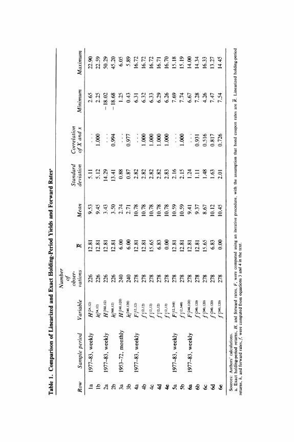
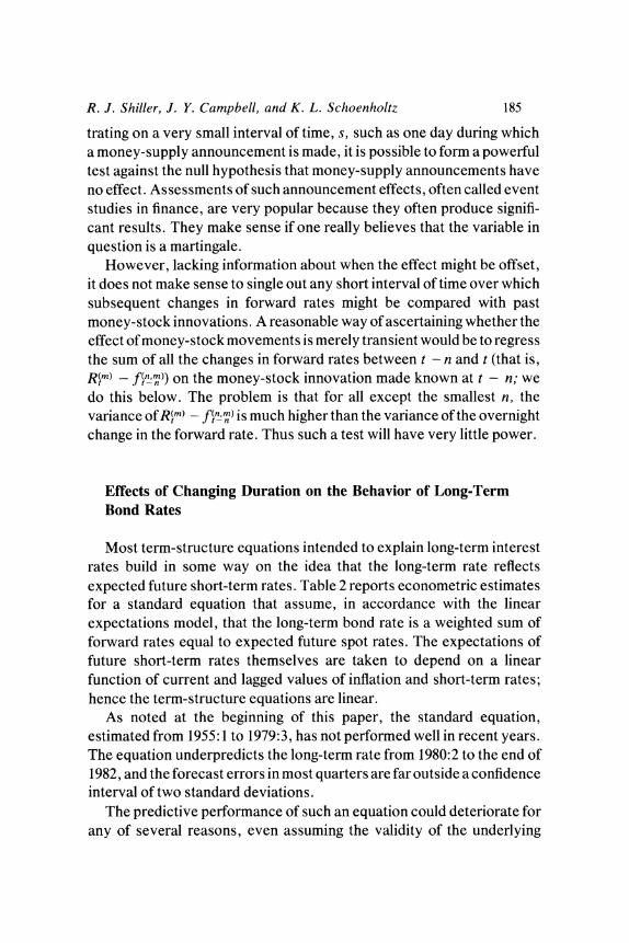
It is important to distinguish tests of the model based on short maturities from tests based on longer maturities. It is plausible that the expectations theory might work better for the shorter maturities. We look first at its value in predicting short-term rates. Figure 1 presents a scatter diagram with data on quarterly changes, 1959:1 to 1982:3, in three-month Treasury bill rates, R3) - R'>3), on the vertical axis and the predicted change, F(3 3) - R(3), implied by the three- and six-month bill rates on the horizontal axis. Measurements are for the first trading day of March, June, September, and December. Our model, which includes
21. Hansen and Sargent, "Exact Linear Expectations Models," and Sargent, "A Note," have used the cross-equation approach. The former paper imposes all the restrictions implied by the expectations theory and rejects the model. However, it is not clear how to interpret the rejection of cross-equation restrictions; Hansen and Sargent state that the expectations model may still be a good forecaster of changes in interest rates. (See note 55 below.)
22. Salomon Brothers, An Analytical Record of Yields and Yield Spreads (New York, 1983).
23. Roll, The Behavior of Interest Rates.
Figure 1. Actual versus Predicted Change in Short-Term Rate, 1959:1-1982:3a Actual change (percentage points)
5 1980:3
4-
3
1979.4
2 a 1980:2
19814 / * /
11981:2 *: * */ Estimated relation 0 l
0 1981:1 1982:
0 01982: @1 98:
,4. . . 1980:4
-l1 / . .* 1982:1 /
Theoretical relation
-2 (actual= predicted)
3 ~~~~~~~~~~~~~1982:2
4-4
-5 @1981:3
1980:1
-4 -3 -2 -1 0 1 2 3 4 Predicted change (percentage points)
Source: Authors' calculations as described in the text, based on data from Salomon Brothers, An Analytical Record of Yields and Yield Spreads (New York, 1983).
a. Quarterly data, ninety-five observations, from the first day of March, June, September, and December. The short-term rate is the three-month Treasury bill rate; the predicted change from the term structure is the three-month ahead, three-month forward rate minus the current three-month rate. The forward rate is computed from the current three- and six-month rates. The predicted change is computed without allowing for a constant risk premium and thus is, by our model, the true predicted change plus a constant. The estimated relation is reported in table 3, row 1.
R. J. Shiller, J. Y. Campbell, and K. L. Schoenholtz 191
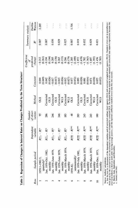
the assumption that expectations are rational, implies that the error terms are uncorrelated in a regression of R(323 - RQ3) on a constant and on 13 3,3) - R(3), and that the slope coefficient is 1.0. The intercept reflects a constant risk premium.24 The dashed line shown is drawn through the sample mean with a slope of 1.0. The estimated regression line (from row 1 of table 3) is the solid line with a negative slope and is almost five standard deviations from 1.0.
We did not attempt to correct for heteroscedasticity over the full sample period because the recent increase in the volatility of interest rates is extreme and does not represent the continuation of a historical trend.25 However, we did adopt a method suggested by Hansen and Hodrick, which allows us to use the full sample of monthly data by correcting the error term for serial correlation.26 Our application of this corrected ordinary least squares estimation method for the period from January 1959 to October 1982 is reported in row 2 of table 3. The use of monthly rather than quarterly data has little effect on the point estimates but does increase their precision. All other results in table 3, with the exception of row 6, are based on monthly data.
To test the conjecture that the expectations model might perform better in the period before the introduction of new Federal Reserve
24. The intercept is important, for note that F(3'3) - RQ3) is, with one important exception, always positive or near zero. If we did not take account of the risk premium, the model would be obviously wrong, as the term structure would nearly always predict increases in interest rates. Before testing the model we must therefore add the risk premium term, Vi, which was mentioned above in connection with equation 1, but was omitted in the text only for expositional simplicity.
25. Glejser suggests a simple method for correcting for error variance which follows a steady time trend. See H. Glejser, "A New Test for Heteroskedasticity," Journal of the American Statistical Association, vol. 64 (March 1969), pp. 316-23. The absolute values of the residuals from a preliminary regression are regressed on both a constant and time; the reciprocals of the fitted values are used as weights in a second regression. Mishkin has applied this method to an earlier sample period. See Frederic S. Mishkin, "Efficient- Markets Theory: Implications for Monetary Policy," BPEA, 3:1978, pp. 707-52, and A Rational Expectations Approach to Macroeconomics: Testing Policy Ineffectiveness and Efficient-Markets Models (University of Chicago, 1983). For the full sample, 1959-82, we found that this method gave almost all the weight to two or three early observations and therefore produced highly erratic results.
26. See Lars Peter Hansen and Robert J. Hodrick, "Forward Exchange Rates as Optimal Predictors of Future Spot Rates: An Econometric Analysis," Journal of Political Economy, vol. 88 (October 1980), pp. 829-53. Quarterly changes in interest rates overlap when sampled monthly. Therefore the error term follows a third-order moving average process, and the estimated coefficient standard errors must take this into account.
S > b O o < ~~~C) > C) C> C
0
C o o 8 o o o
?> c; o ; o; o ,oooooo;
= U t t t N w_ _ N N > t~~~~~~~~~~~~~k) C'sNo ->o t
Su~ ~ ~~~~I c- kO O OOOO OC kO en O O ,
L oY~~~~~~~~~~~~~~~~~~~~~~~~~~~~~~~, Yo 0o
;0 U) Cs
X _, X S:: ON 00 "t 00 Io t ?? "t It ??0
= % > 4 cs cs cs _ _ =, 8 ct~~~~~~~~~~~~~~~~~~~~~~~~~~~~~~~~~~~~~~~~~~~~~~~~~~~~~~~~~~~~'
V Qk
O 8 n~~~~~~~~~~~~~~~~~~~~~~~~~~~~~~~~~~~~~~~~~~~~C X _ _ _ i S i 3 i E <~~~~~~~~~~~~~~~~~~~~~~~~~~~~~~~~~~C
Y =:, ffi < <- <- <- ea: < ? < _ < vl Q~~~~~~~~~~~~~~~t
X o ~~~~ ~~CN CN CN C h Y CN
n
o - N < t tn ? > oo
~~~~~~~~~Crso:Z L} C
F t _ U) Y = e D Q~~~~~~~~~~~~C
R. J. Shiller, J. Y. Campbell, and K. L. Schoenholtz 193
operating procedures in October 1979, we shortened our sample and repeated our regression tests with and without a heteroscedasticity correction (rows 3 and 4 of table 3). The negative slope for the entire sample period is due primarily to recent observations. When we drop these observations, the slope coefficient becomes positive; but it is insignificantly different from zero and significantly different from 1.0.27
This result is not altered by further shortening of the sample period to exclude the unusual period of volatile interest rates in 1974-75 (row 5).28
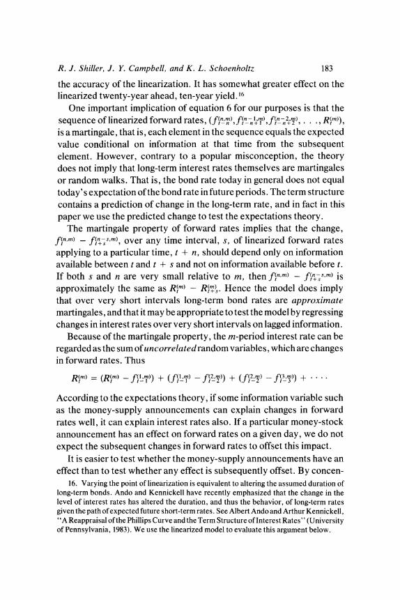
The situation is, if anything, worse for long-term bond rates. Figure 2 shows a scatter diagram with changes over a six-month interval in thirty- year, or 360-month, bond yields, RQ60) - R(360), on the vertical axis and on the horizontal axis the predicted change, f(6,354) - Ri360)), implied by the 360-month yield and the six-month yield at the beginning of the six- month period. The R used to compute the linearized forward rates was 6.65 percent a year. Once again, the model implies that the error terms are serially uncorrelated in a regression of R(160) - Ri360) on a constant and f6,154) - M160), and the theoretical slope coefficient is 1.0.29 Thus a simple regression test is an appropriate way to test for market efficiency with long-term bonds. Such a test may be regarded as a "forward- filtered" test, as defined by Hayashi and Sims, of the model of equa-
27. The estimated coefficient resembles the coefficient in a similar regression by Hamburger and Platt (their equation 5). However, these authors inexplicably conclude in favor of the expectations model. See Michael J. Hamburger and Elliott N. Platt, "The Expectations Hypothesis and the Efficiency of the Treasury Bill Market," Review of Economics and Statistics, vol. 57 (May 1975), pp. 190-99.
28. More favorable results for the simple expectations model were found in Shiller, using data on six- and twelve-month 1.5 percent Treasury notes (Series EA and EO) and a slightly earlier sample. (Shiller, "Alternative Tests of Rational Expectations Models.") The more favorable results were not due to the slightly different sample or to the slightly different maturities. Using regression diagnostic procedures described by Belsley, Kuh, and Welsch, it was found that the results in that paper were heavily influenced by the 1970- I and 1970-11 observations. See David A. Belsley, Edwin Kuh, and Roy E. Welsch, Regression Diagnostics: Identifying Influential Data and Sources of Collinearity (Wiley, 1980). As confirmed by the Commercial and Financial Chronicle for those dates, the yields on these Treasury notes were behaving erratically at that time. As noted in Shiller, quantities of the Treasury notes outstanding fell below $100 million after 1969, and the "thin" markets made price data less reliable. (Shiller, "Alternative Tests of Rational Expectations Models.") When the same regressions in that paper were run truncating the sample at 1969-II, they confirmed the negative results for the expectations theory reported here.
29. We approximated here by ignoring the difference between R'354' and R'360'.

Figure 2. Actual versus Predicted Change in Long-Term Rate, 1959-82a
Actual change (percentage points)
a 1980.2
1981:1 a
Estimated relation 1982:1 *
1981:2- * . _ ; '. .*
0 -~ ~ ~ ~ ~ ~~~~~~00 Theoretical relation 0 * 1 9 80. (actual = predicted)
2-1
-3 0 1982:2
-0.20 -0.15 -0.10 -0 05 0.00 0.05 0.10 0.15 Predicted change (percentage points)
Source: Same as figure 1. a. Semiannual data, 1959-82, forty-eight observations from the first day of January and July. The long-term rate
is the thirty-year Treasury bond rate; the predicted change from the term structure is the six-month ahead, thirty- year linearized forward rate minus the current thirty-year rate. The forward rate is computed from the current six- month and thirty-year rates. Predicted change is computed without allowing for a constant risk premium and thus is, by our model, the true predicted change plus a constant. The estimated relation is reported in table 3, row 6.
R. J. Shiller, J. Y. Campbell, and K. L. Schoenholtz 195
tion 1.30 However, it is possible that other tests, such as the "volatility tests" developed by Shiller in his 1979 paper, may have more power. Shown are a dashed line drawn through the sample mean with a slope of 1.0 and a solid line for the regression. As in the case of the short-term rates, the results of the test do not support the theory: when long-term rates are predicted to rise, they in fact tend to go down.
The predicted six-month change in the thirty-year bond rate is approximately the spread between the thirty-year bond yield and the six-month rate, divided by the duration (measured in six-month intervals) of a thirty-year bond minus 1.0. The magnitude of the estimated coeffi- cient thus depends on the R used to compute duration. If, for example, we had chosen R = 3 percent rather than 6.65 percent, the duration given by equation 2 would rise from fourteen to twenty years, and the estimated coefficient would be multiplied by 20/14 = 1.43. But changing the duration used could never change the sign of the coefficient.
The variance of the predicted change in long-term rates in figure 2 is much smaller than the variance of the actual change, so the probability of rejecting the hypothesis that the slope is 1.0 if the slope term is actually zero (in statistical terms, the power) is low. The horizontal axis in the figure had to be drawn on a different scale than the vertical (as shown by the flatter appearance of the dashed line). Had they been on the same scale, the scatter of points would be so close together horizontally that they would be indistinguishable.
The estimated coefficients for thirty-year bond rates in table 3 are always negative; but reflecting the low power of the tests, they have extremely large standard errors. Nevertheless, our use of monthly data gives the estimates some additional precision, and we are able to reject at the 4.5 percent confidence level the hypothesis that the coefficient is 1.0 in row 8. This regression corrects for moving-average errors but does not correct for heteroscedasticity; when we perform weighted least squares we still reject at the 5.5 percent level in row 9. These results confirm for a shorter but more frequently sampled period the regression tests reported in Shiller.3"
The standard deviation of the actual change in interest rates is about
30. Fumio Hayashi and Christopher Sims, "Nearly Efficient Estimation of Time Series Models with Predetermined, but not Exogenous, Instruments," Econometrica, vol. 51 (May 1983), pp. 783-98.
31. Shiller, "Volatility of Long-Term Interest Rates."

196 Brookings Papers on Economic Activity, 1:1983
two and a half times the standard deviation of the predicted change for the short-term interest rates in figure 1 and about fourteen times the standard deviation of the predicted change for the long-term interest rates in figure 2. Thus under the null hypothesis that the true slope coefficient is 1.0, the R2 of the regressions ought to be small: about 1/[(2.5)2] = 0.16 for the short-term rate regression, about 1/[(14)2] =
0.005 for the long-term. At least for the short-term rate regression the R2 value is large enough that a test of the null hypothesis against an alternative that R2 equals zero should have some power.
Under the null hypothesis, the standard deviation of the estimated coefficients in an ordinary least squares regression should be about 2.5/[N(0 5)] for the short-term rate regressions and 14/[N(0 5)] for the long- term rate regressions, where N is the number of observations. There are ninety-five observations in figure 1 and forty-eight observations in figure 2, implying standard errors of roughly 0.25 and 2.0, respectively. Thus we easily reject the short rate regression at conventional levels because there is no apparent relation between actual and predicted changes. We also reject at this level for the long-term rate regressions that use the more numerous monthly observations; for these regressions the esti- mated coefficients are decidedly negative.
To summarize these results, the sample evidence is not for the hypothesis that the slope of the term structure correctly forecasts future changes in interest rates. This behavior of long-term bond rates has straightforward implications for optimal financing decisions of corpora- tions and individuals who are concerned purely with expected returns. According to the expectations theory, such investors should be indiffer- ent about investing "long" or "short." The results suggest, contrary to the theory, that the six-month returns to holding bonds are higher than on bills when the bond rate is relatively high. For example, row 8 of table 3 implies that such an investor would prefer to buy thirty-year Treasury bonds rather than six-month Treasury bills whenever the thirty-year yield exceeds the six-month yield by 75 basis points or more.
From 1959 to 1982, such a risk-neutral investor would have been long approximately 45 percent of the time. The slope of the term structure is a sufficiently good predictor of excess returns to overcome the fact that average returns on long-term bonds have been lower than on short-term bonds. The current spread of over 200 basis points makes long invest- ments preferable by a considerable margin. By this reasoning, companies

R. J. Shiller, J. Y. Campbell, and K. L. Schoenholtz 197
should delay long financing until long-term rates fall relative to short- term rates, and householders should not switch from floating to fixed rate mortgages until this occurs.32 It is perhaps surprising only to students of the expectations theory that this is what a naive person might have done without the guidance of a sophisticated model.33
Of course, the participants in the bond market may well be concerned with risk as well as with expected returns, and our rejection of the simple expectations theory could be attributed to variations in risk premiums that are so large as to destroy any information in the term structure about future interest rates. Such an explanation is in closer accordance with current theoretical predispositions than one that points to "irrational" markets. However, lacking any theoretical restrictions on the variation in risk premiums, these hypotheses cannot be distinguished.
Two approaches might preserve the relevance of the expectations model by embedding it in a more general theory. One possibility is to specify a time-varying risk premium in terms of observed data, a method we employ below. Another is to suppose that the risk premium moves slowly enough that extremely short-term movements in yields (as between trading days before and after a money announcement) can still be understood in terms of a simple expectations model. We have no tangible evidence, of course, that the risk premiums do not move from one day to the next.
Time-Varying Risk, Variability of Interest Rates, and Credit Volume
Systematic differences between the long-term rate and the expected value of future short-term rates have been given many names: risk premium, liquidity premium, habitat effect, market segmentation effect,
32. This prescription is valid only if our results for government securities carry over to private debt.
33. Some economists have offered suggestions for corporate financing that are designed to achieve tax savings, but these depend crucially on the expectations theory of the term structure. For example, Roger Gordon argues that corporations should issue short-term debt when short-term rates are high to accelerate tax deductible interest payments. See Roger H. Gordon, "Interest Rates, Inflation, and Corporate Financial Policy," BPEA, 2:1982, pp. 461-88. Our results suggest it is not surprising that few corporate treasurers heed such advice.
~~- - - 0 0~~~~~~t- - 00 -
Cq~ ~ ~ ~~~~~~C
S N ? ^ F o X NNCN W
000 00ONWC 0 00
000000 ~~~.C00 ma,00
tc 00 00 0r ~ t-0r1 z
m On .3 1 m CN CN O *1 *t cn r- "
N
t. ~ ~ ~ - -- . -o? . .
on un V on on on o o
C) Cq C) I) C ) )
o U m0 0 0 0
0
CN CN~~~~~O Cq o o o ooooooN 0 ON ON ONO ̂ O O O
N. - NN 0C
E ~ ~ O ON QZQZQ
X~~~~~~~~~~~~~~~~~~~~~~~0 O
cnC6
V s s w
m~~~~~ > < _ e R t -_ .
0 ~ ~ - t.5ON I)O I) N I ~ \0O \0O 1
E b U ?_ ?_ ?_ e_ e_ e+ e+ i+ s0) &
*E~~c t t N t 0..tt
Pw~~~~~~~~~~~~~~~~~~i c 0

R. J. Shiller, J. Y. Campbell, and K. L. Schoenholtz 199
and so on. Here we model changes in this discrepancy as reflecting changing levels of uncertainty. Suppose we add a risk premium term, Vit, to the model in equation 1. The one-period excess holding return on an i-period bond, hfi I) - RM, then equals DiVi, - (Di - 1) E,Vi ,+I plus noise unforecastable at time t. By regressing the difference between h(i, l and RM') on observable and relevant variables, we can then estimate the risk premium. If i = 2, then Vi1,t+1 is zero by definition and the value of the excess holding return predicted by the regression divided by D2 (or roughly 2) may be regarded as an estimated V2,. This method of estimating the risk premium was proposed by Kessel.34 If i is very large and if Vit = EtVi 1,t+ I is assumed, the value predicted by the regression is itself an estimate of Vit.
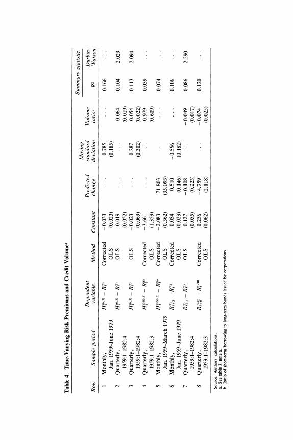
A number of earlier studies of the term structure have used an eight- quarter moving standard deviation of the three-month Treasury bill yield as an ad hoc measure of time-varying risk.35 Row 1 of table 4 shows that this variable is indeed significant in predicting excess three-month returns on six-month Treasury bills for the sample period, 1959-79. We found that the moving standard deviation was much less successful in predicting excess returns on long-term bonds (perhaps because of the much higher variance of these returns and their persistent tendency to be negative during 1959-79). Therefore we do not report regressions with this variable for long-term bond returns.
The moving standard deviation proxy for risk is not derived from any well-articulated economic theory. In fact, the basic message of standard finance models is that it is not the volatility of asset returns but their covariance with other asset returns or underlying factors that determines their "riskiness." Further, the empirical results are not robust. The risk variable becomes much less significant if the sample period is extended to include the last three years or if a simple moving standard deviation
34. Reuben A. Kessel, The Cyclical Behavior of the Term Structure of Interest Rates (National Bureau of Economic Research and Columbia University Press, 1965). Kessel in fact used the difference between the forward rate and the subsequent spot rate as the dependent variable in his regression, but inspection of equations 3 and 4 shows that this difference is a constant multiple of the excess holding return.
35. This tradition seems to have started with Modigliani and Shiller, "Inflation." The variable has also been used by, among others, Ando and Kennickell, "A Reappraisal"; by Jones and Roley in David S. Jones and V. Vance Roley, "Rational Expectations, the Expectations Hypothesis and Treasury Bill Yields: An Econometric Analysis," Working Paper 869 (National Bureau of Economic Research, June 1982); and by Mishkin, A Rational Expectations Approach.
200 Brookings Papers on Economic Activity, 1:1983
is replaced by a predictor of the variance of the innovation in the three- month bill rate.
The conceptual inadequacy of the standard variable that is thought to measure time variations in risk suggests that it may be worth seeking alternatives. It is widely believed that the volume of short- and long- term debt issue, the level of rates, and the shape of the yield curve are all jointly determined. Economists have long argued about the merits of "preferred habitat" theories in which borrowers and lenders, because of their particular needs, prefer to enter the market at different maturi- ties. The belief that excess return may be required to induce investors to move from their preferred habitat is itself a basis for policymakers to believe that they may be able to twist the yield curve by government debt management. Recently Friedman and Roley have pursued research programs based on the premise that supply and demand curves for debt are econometrically identifiable.36 They have sought to isolate factors that shift one curve without affecting the other.
Our more modest goal here is to see if a volume variable that measures the relative amount of activity in the short end of the market compared to the long end helps to predict risk premiums as we have defined them. In row 2 of table 4 we regress excess returns on six-month bills on the previous quarter's ratio of short borrowing to long financing by U.S. corporations.37 This volume ratio may be related to market perceptions of the risk in longer-term bonds but can show either a positive or a negative relation to the risk premium, depending on whether borrowers or lenders are more adversely affected. The volume ratio is indeed a significant predictor of excess returns for 1959-82, and if it is included in a regression along with the moving standard deviation (row 3), we find that the volume ratio dominates the conventional measure of risk.
36. See especially Benjamin M. Friedman, "Financial Flow Variables and the Short- Run Determination of Long-Term Interest Rates," Journal of Political Economy, vol. 85 (August 1977), pp. 661-89, and "Substitution and Expectation Effects on Long-Term Borrowing Behavior and Long-Term Interest Rates," Journal of Money, Credit and Banking, vol. 11 (May 1979), pp. 131-50; and V. Vance Roley, "The Determinants of the Treasury Security Yield Curve," Journal of Finance, vol. 36 (December 1981), pp. 1103- 26, and "Asset Substitutability and the Impact of Federal Deficits," Working Paper 1082 (National Bureau of Economic Research, February 1983).
37. These data are ultimately derived from the U.S. flow-of-funds accounts, but were aggregated for us by Salomon Brothers. Following the flow-of-funds convention, short borrowing is of maturity less than one year, and long financing is all other borrowing.

R. J. Shiller, J. Y. Campbell, and K. L. Schoenholtz 201
However, it is not significant over the shorter and earlier sample period, 1959-79. The volume ratio is significant only at the 10 percent level in predicting excess returns on long-term bonds (row 4).38
The fitted values from these regressions give our best estimates of risk premiums. How do these estimates change over time? Consider row 1 of table 4. The moving standard deviation of annualized three-month bill rates averaged 70 basis points over the twenty-year period from 1959 to 1979. In 1979-82 it increased from about 140 basis points in early 1979 to a high of over 250 basis points in late 1981 and in 1982. According to the regression of table 4, row 1, this implies that the expected excess holding return on six-month bills was 55 basis points higher than the previous average in 1979, and 140 basis points higher in 1982. Adjusting for duration, this means that the risk premium in the six-month bill rate was about 27.5 basis points higher in 1979 and 70 basis points higher in 1982 than in the previous twenty years.
For long-term bond rates the moving standard deviation proxy for risk is less successful. An alternative is to treat the spread between the six-month and thirty-year rates as a risk proxy and ask what risk premium was implied by the maximum 1982 spread of 2.5 percent. The answer to this question is contained in the regression of table 4, row 5. There excess holding returns on thirty-year bonds are regressed on the pre- dicted change in thirty-year rates. This predicted change variable is just the spread divided by the duration of a thirty-year bond (which in the 1959-79 sample period averaged 13.5 years or 27 six-month time units) minus one. The coefficient of 71, divided by 26, implies that on average when the spread is 1 percent, the risk premium in the long-term rate is 2.7 percent. Given the 1982 maximum spread of 2.5 percent, our regression suggests that the risk premium peaked at 6.8 percent. The very large values of the estimated risk premiums seem implausible, but of course they are necessary if we are to interpret the term structure in these terms. The risk premium must move enough to explain the perverse behavior of the term structure in predicting future long-term interest rates.
Finally, we can ask whether the risk variables of this section improve the expectations model as might be hoped. Rows 6, 7, and 8 of table 4
38. Our success with this crude measure of relative volume by maturity suggests that policymakers would benefit from more frequent and accurate collection of data summariz- ing credit volume.

202 Brookings Papers on Economic Activity, 1:1983
represent rows 3, 1, and 6, respectively, from table 3 with risk variables added.39 We hoped that the addition of these variables would bring the coefficient of the predicted change closer to 1.0. In fact, the coefficient is only slightly closer to 1.0 for the short-term rate and farther from 1.0 for the long-term rate.
Money Announcements and the Term Structure of Interest Rates
The tendency for interest rates to rise suddenly after an announcement of an unexpectedly large money stock has been widely noted. Some have interpreted this effect of a surprise money announcement as implying that expansionary monetary policy actually raises interest rates through its anticipated effect on inflation rather than lowering them through a liquidity effect as traditional Keynesian theory would predict. In this section we describe the money-surprise effect and also refine the interpretation of it. We argue, for example, that it is quite wrong to interpret the response to money surprises as disproving the Keynesian liquidity effect on interest rates.
Figure 3 displays on the vertical axis the change in a short-term interest rate plotted against, on the horizontal axis, the surprise in the money stock for each week between February 1980 and February 1983. To calculate the money-surprise variable one needs a measure of the actual and the expected money stock. The money stock selected corre- sponds to the unrevised narrow measure of money emphasized by the Federal Reserve (MIB, renamed MI in January 1982). The money-stock announcement occurred in our sample on Fridays at 4:10 p.m. The expected money measure employed is the Tuesday median forecast of the money stock from the weekly market survey of Money Market Services, Inc. In the figure the money surprise is the difference between the actual and expected money stocks.
Several authors, including Cornell and Roley, have sought to evaluate the efficiency of the Money Market Services forecast.40 They have shown that the forecast is efficient with respect to information sets
39. Slight sample changes were necessitated by the quarterly measurement of the volume ratio.
40. Cornell, "Money Supply Announcements," and Roley, "The Response of Short- Term Interest Rates."

Figure 3. The Money-Announcement Effect, February 1980 to February 1983
Change in interest rate, in basis points 200
150
100 * 0
00 ~ **
50- Estimated relation
0
..0e
-50 0
.0
-100 _
- 150 -5 0 5
Money surprise, in $ billions Source: Authors' calculations as described in the text, with data from the Board of Governors of the Federal
Reserve System and Money Market Services, Inc. a. Weekly data, with some weeks omitted because of holidays; 132 observations from 1980 (eighth week) to 1983
(fourth week). The interest rate is the three-month Treasury bill rate. Its change is measured from 3:30 p.m. on Friday to 3:30 p.m. on Monday. The money-surprise variable is the difference between the money stock announced on Friday, in $ billions, and the previous Tuesday's median forecast of the money stock from the weekly survey conducted by Money Market Services, Inc. Also shown is the regression line reported in table 5, row 3.

204 Brookings Papers on Economic Activity, 1:1983
containing the lagged forecasts and current and lagged interest rates. In addition, it generates a lower root mean squared error in prediction than an (ARIMA) model based on observed money stocks. We do not reproduce these tests but we can confirm that there is no significant serial correlation in the forecast errors.
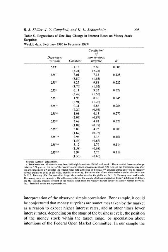
The vertical axis displays the change in the three-month Treasury bill interest rate in basis points from Friday at 3:30 p.m. until Monday at 3:30 p.m. The diagonal line is a simple regression through the observa- tions. The regression portrayed in this figure is found in row 3 of table 5, which also shows the results for yields ranging from the federal funds rate (denoted FF) to the thirty-year Treasury bond yield. The coefficient of the money surprise is measured in basis points per $ billion surprise, with the standard deviations in parentheses. It is apparent from the table that the money announcement has a significant, albeit declining, effect throughout the entire term structure.41 This reconfirms the work of other authors for our more recent data sample.
Previous authors have stressed the statistical significance of these results. However, the R2 values in the table 5 regressions do not exceed 0.286; money surprises explain only a small fraction of the changes in interest rates from Friday to Monday. Furthermore, the sample variance of interest rates from Friday to Monday for our sample from August 1980 to July 1983 is only one-third of the weekly variance in interest rates (measured from either Friday to Friday or Monday to Monday). Hence if the yields approximate a random walk over the week, the regressions explain only 3 to 10 percent of the weekly movement in the rates. It is only by concentrating the period of observation closely around the announcement that results of this magnitude can be obtained. This is an example of the general problem with event studies discussed above. Because R2 is so low, the theory does not explain much of what is happening; moreover, there is room for a wide variety of explanations involving unobserved variables, which might significantly alter the
41. An alternative measure of the money-stock forecast error suggested by Roley was also employed. This involves regressing the Money Market Services, Inc., forecast error on the change in the three-month interest rate from Tuesday to Friday (to account for new information available between the forecast and the money-stock announcement) and to use the residuals from this regression as the exogenous variable in the table 5 regression. Because the results closely approximate the regressions displayed in table 5, we do not report them.
R. J. Shiller, J. Y. Campbell, and K. L. Schoenholtz 205
Table 5. Regressions of One-Day Change in Interest Rates on Money-Stock Surprises Weekly data, February 1980 to February 1983a
Coefficient of
Dependent money-stock variable Constant surprise R2
AFF - 1.12 7.86 0.086 (5.21) (2.25)
AR"M 7.01 7.13 0.128 (3.80) (1.63)
AR(3) 4.25 9.88 0.222 (3.76) (1.62)
AR(6) 6.11 9.32 0.228 (3.49) (1.50)
AR(12) 1.96 8.16 0.245 (2.91) (1.26)
,5,R(24) 0.31 6.86 0.286 (2.20) (0.95)
A_R(36) 1.08 6.13 0.275 (2.03) (0.87)
A-R(60) 2.68 4.83 0.227 (1.82) (0.78)
AR(84) 2.80 4.22 0.209 (1.67) (0.72)
AR(120) 2.96 3.36 0.161 (1.56) (0.67)
AR(240) 3.12 2.79 0.114 (1.58) (0.68)
AR(360) 2.94 2.75 0.119 (1.53) (0.66)
Source: Authors' calculations. a. Data based on 132 observations from 1980 (eighth week) to 1983 (fourth week). The A symbol denotes a change
between 3:30 p.m. on the day of the weekly money-stock announcement and 3:30 p.m. on the first trading day after the announcement; FF denotes the federal funds rate at the end of the day; RQJ) denotes annualized yield to maturity in basis points on bond or bill with j months to maturity. For maturities of less than twelve months, the yields are for U.S. Treasury bills. For maturities longer than twelve months, the yields are for U.S. Treasury notes and bonds. The money surprise variable is the difference between the money stock announced on Friday in billions of dollars and the Tuesday median forecast of the money stock from the weekly market survey of Money Market Services, Inc. Standard errors are in parentheses.
interpretation of the observed simple correlation. For example, it could be conjectured that money surprises are sometimes taken by the market as a reason to expect higher interest rates, and at other times lower interest rates, depending on the stage of the business cycle, the position of the money stock within the target range, or speculation about intentions of the Federal Open Market Committee. In our sample the
206 Brookings Papers on Economic Activity, 1:1983
former circumstance might simply have occurred more frequently than the latter.42
Other research on the money-announcement phenomenon has ex- amined a number of questions that we have left aside. For example, Roley has examined the change in Federal Reserve policy in October 1979, and has found that the money-announcement effect was much weaker and less significant before that date. We would like to be able to determine whether the effect weakened in late 1982 due to a policy shift toward stabilizing the federal funds rate, but we do not yet have sufficient data. Roley has also examined potential nonlinearities such as the effect of money-stock innovations that lie outside the identified target bounds of the Federal Reserve for monetary growth. Urich and Wachtel also examined the effect of price-index announcements on interest rates but found relatively weak effects.43
The results above showing that money surprises have a significant impact on long-term bond rates do not indicate whether this simply reflects the effect on the current short-term rate in equation 1 or whether forward rates further in the future are also affected. In table 6 we estimate the effect of money surprises on forward rates (calculated according to equation 4). Hardouvelis examined the same effect in a recent unpub- lished paper but, in the absence of a formula for calculating the forward rate on coupon-carrying bonds, treated the yields on Treasury issues as pure discount bonds."4 As can be seen from equation 4, this places
42. The effect of the money-stock innovation might seem even less impressive when one considers Grossman's observation that there has been virtually zero correlation between initially announced weekly money-stock changes and the final, revised data on changes in the money stock. See Jacob Grossman, "The 'Rationality' of Money Supply Expectations and the Short-Run Response of Interest Rates to Monetary Surprises," Journal of Money, Credit and Banking, vol. 13 (November 1981), pp. 409-24. Maravall and Pearce found that preliminary data on two-month growth rates of MI gave wrong signals as to whether MI growth rates were in the tolerance range of the Federal Open Market Committee 40 percent of the time. See Agustin Maravall and David A. Pearce, "Errors in Preliminary Money Stock Data and Monetary Aggregate Targeting," Special Studies Paper 152 (Board of Governors of the Federal Reserve System, 1980). However, they attributed the versions primarily to changing seasonal factors. Since the Census X-1 1 program used to deseasonalize data is publicly known, there is still good reason to believe that the forecast errors represent genuine errors in predicting the money supply before deseasonalization.
43. Urich and Wachtel, "Effects of Inflation and Money Supply Announcements." 44. Gikas Hardouvelis, "Market Perceptions of Federal Reserve Policy and the Weekly
Monetary Announcements, " Working Paper (University of California at Berkeley, 1982).
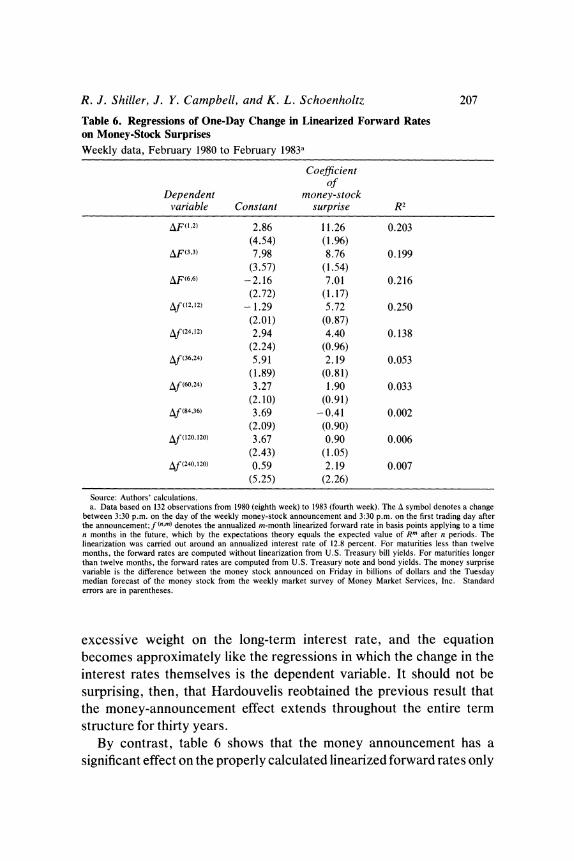
R. J. Shiller, J. Y. Campbell, and K. L. Schoenholtz 207
Table 6. Regressions of One-Day Change in Linearized Forward Rates on Money-Stock Surprises Weekly data, February 1980 to February 1983a
Coefficient of
Dependent money-stock variable Constant surprise R2
AF(1,2) 2.86 11.26 0.203 (4.54) (1.96)
A&F(3,3) 7.98 8.76 0.199 (3.57) (1.54)
AF(6,6) --2.16 7.01 0.216 (2.72) (1.17)
Af (12,12) - 1.29 5.72 0.250 (2.01) (0.87)
Af (24,12) 2.94 4.40 0.138 (2.24) (0.96)
Af(36,24) 5.91 2.19 0.053 (1.89) (0.81)
Af(60,24) 3.27 1.90 0.033 (2.10) (0.91)
Af(84,36) 3.69 -0.41 0.002 (2.09) (0.90)
Af (120, 120) 3.67 0.90 0.006 (2.43) (1.05)
Af(240,120) 0.59 2.19 0.007 (5.25) (2.26)
Source: Authors' calculations. a. Data based on 132 observations from 1980 (eighth week) to 1983 (fourth week). The A symbol denotes a change
between 3:30 p.m. on the day of the weekly money-stock announcement and 3:30 p.m. on the first trading day after the announcement; f (n,m) denotes the annualized m-month linearized forward rate in basis points applying to a time n months in the future, which by the expectations theory equals the expected value of R- after n periods. The linearization was carried out around an annualized interest rate of 12.8 percent. For maturities less than twelve months, the forward rates are computed without linearization from U.S. Treasury bill yields. For maturities longer than twelve months, the forward rates are computed from U.S. Treasury note and bond yields. The money surprise variable is the difference between the money stock announced on Friday in billions of dollars and the Tuesday median forecast of the money stock from the weekly market survey of Money Market Services, Inc. Standard errors are in parentheses.
excessive weight on the long-term interest rate, and the equation becomes approximately like the regressions in which the change in the interest rates themselves is the dependent variable. It should not be surprising, then, that Hardouvelis reobtained the previous result that the money-announcement effect extends throughout the entire term structure for thirty years.
By contrast, table 6 shows that the money announcement has a significant effect on the properly calculated linearized forward rates only

;::
a ~~~~~~~~~~~~2 2
4) V -
S~~~~~~~~~~~~~~~~~~~~~~~~~~~~~~~~~~~~~~~~~0 V X b
tos,~~~~~~~~~~~~~~~,
O .77? . 0 .-=e; S a 0 i . -x _ C y ] F Q~~~~~~~~~~~~~~~~~~~~~~~~I -a
0
| ,., : ,'.::t'2 = g
S ~ ~ ~ ~ ~ ~ ~ ~ ~ ~ ~ ~ ~ ~ ~ ~ ~ ~ ~~~~~4 NidS > '= i ;\L,\ ie,\ .\ R i = .E~~~~~~ ::s T~~~~~~~~~~~~~~~~~~~~~~02SA 4, a ,
UZ t 2 2 As -est~~~~~~~~~~~~~~~4 E~~~~~~~~~~~~~~~~~~~~~~~~~~- 4) eXE
; ? o u o u o u ~~0 X

R. J. Shiller, J. Y. Campbell, and K. L. Schoenholtz 209
as far as the five-year ahead, two-year rate.45 Indeed, the explanatory power of the regression, as measured by R2, tapers off significantly after the two-year ahead, one-year rate. These results are displayed in figure 4, in which the horizontal axis measures years from the present and the vertical axis represents the forward rate changes in basis points per $ billion surprise. The horizontal segments in the heavy line correspond to the forward rates beginning at the left end of the segment and extending to the right end. The shaded area identifies a two-standard-deviation bandwidth on either side of the point estimate of the effect. The display begins with the one-month Treasury bill rate and shows all subsequent forward rates for the twenty-year ahead, ten-year rate.
How is one to interpret this money-surprise effect? It is instructive first to consider the effect of money surprises on the shortest interest rate, the federal funds rate. This requires an awareness of some basic institutional facts about the current regime of monetary control. Under the system of lagged reserve accounting, banks must hold reserves in a given statement week (Wednesday to Wednesday) to cover their deposits of two weeks earlier.46 This lag is the same as the delay in reporting the level of Ml. Furthermore, banks can hold their reserves on any day of the statement week so long as the average over the week is at least at the required level (and subject to the constraint that random shocks should not exhaust their reserve account at the Federal Reserve).
On any day the federal funds rate may be thought of as the price of bank reserves on that day. If we disregard excess reserves (which are generally small), the aggregate demand schedule for reserves on Wednes- day, the last day of the statement week, is vertical.47 Demand for reserves
45. Once again, the standard errors appear in parentheses. The notation DF (60,24) refers to the change in the sixty-month ahead, twenty-four month rate from Friday at 3:30 p.m. to the following Monday at 3:30 p.m. For maturities up to twelve months the forward rates are computed without the linearization from Treasury-bill yields. For maturities of twelve months or more the forward rates are computed from Treasury note and bond yields, using a point of linearization of 12.8 percent. The results of table 6 are not greatly affected if the forward rates are computed with the current thirty-year bond rate at each point in time as the point of linearization.
46. This system is scheduled to be replaced by contemporaneous reserve accounting in 1984. As shown below, this change will alter the response of the federal funds rate to money-stock announcements.
47. This also ignores the possible effects of a provision allowing banks to carry excess reserves forward or to make up a reserve deficiency the following week. Such carry-over is limited to 2 percent of a bank's required reserves.

210 Brookings Papers on Economic Activity, 1:1983
is completely inelastic because it is determined by reserve requirements arising from deposits of two weeks earlier and by the fraction of reserve requirements already fulfilled on earlier days of the statement week. Demand for reserves over any portion of the statement week ending on Wednesday is completely inelastic for the same reason.
The supply schedule for aggregate reserves is determined by the Federal Reserve because it is the only source of aggregate reserves. The federal funds rate may be regarded as a proxy for the total cost of borrowing from the Federal Reserve. The funds rate is then the discount rate plus the nonpecuniary costs ("frowns") that are imposed by the monetary authority on borrowers at the discount window. The supply schedule is upward sloping since the frowns increase with the amount borrowed.
The intersection of the vertical demand schedule and the upward sloping supply schedule for reserves determines the federal funds rate independently of the current demand for money. Indeed some have argued that, under lagged reserve accounting, the stock of money this week is determined only by the public demand for money at the current funds rate, since banks' supply schedule for money is infinitely elastic at this funds rate.48
At the beginning of the statement week individual banks are interested in forecasting the federal funds rate in the last portion of the week. They could profit from being able to predict, say, an increase in the funds rate, since they average their reserves over the week in fulfilling their reserve requirements and they could plan to hold required reserves early in the week and lend reserves later. But early in the statement week these banks know neither the position of the demand curve for aggregate reserves nor the position of the supply curve for aggregate reserves at the end of the week. The position of the demand curve is uncertain in part because, while each bank knows its own deposits, it does not know the aggregate deposits from two weeks earlier against which the banking system must hold reserves this week. The position of the supply curve is unknown, even though banks may have some idea about its slope, because they do not know this week's aggregate nonborrowed reserves.
The announcement of the money stock from two weeks earlier, which
48. Robert L. Hetzel, "The October 1979 Regime of Monetary Control and the Behavior of the Money Supply in 1980," Journal of Money, Credit and Banking, vol. 14 (May 1982), pp. 234-51.

R. J. Shiller, J. Y. Campbell, and K. L. Schoenholtz 211
occurs in the middle of the statement week, then carries information about aggregate required reserves and the position of the reserve demand curve for the remainder of the statement week. If the money stock in any week is determined by demand, the money surprise this week is a surprise only about the demand for money two weeks earlier, and not about the supply of money at that time. But the money surprise carries information about the current supply curve for reserves. Since the federal funds rate is observed continually, the height of the intersection of current reserve demand and supply curves is known before the announcement, and thus information about one curve is also information about the other. A similar point was made by Nichols, Small, and Webster in the context of a rather different model.49
It is hard to be more precise about the behavior of the federal funds rate over the statement week without becoming involved in more intricacies than are appropriate for this paper. A properly specified rational expectations model of the federal funds market (and the market is one for which rational expectations seem most appropriate) would have to provide detailed sources of information unfolding over the statement week: for example, the level of reserves from a week ago, announced on Friday. The model would also have to take account of the role of the federal funds rate in aggregating the private information of individual banks about their own reserve requirements.
We think, though, that this discussion lends plausibility to several important points. First, the rise in the funds rate in response to a positive money surprise provides no evidence that a decision of the Federal Reserve to increase reserves will raise short-term interest rates. Second, the money surprise is information both that the demand for money two weeks ago was higher than expected and that Federal Reserve policy is now more expansionary than expected. Third, the increase in the funds rate may reflect nothing more than an expected scramble for reserves at the end of the statement week. Finally, the funds rate should follow an approximate random walk over the statement week. If the funds rate deviated systematically from a random walk, for example, if it were persistently higher on any day of the week, then fewer banks would want to hold reserves on that day. Since aggregate reserves cannot be reduced (except to the extent that the banking system borrows less
49. See Nichols, Small, and Webster, "Why Interest Rates Rise."
212 Brookings Papers on Economic Activity, 1:1983
at the discount window), such a situation cannot be an equilibrium.50 If the funds rate is indeed a random walk, information received on Friday that the rate will be higher on Wednesday should cause it to increase immediately.
Examination of the federal funds rate on a daily basis from January 1977 to February 1983 leads to some doubt about the random walk hypothesis. If we partition the sample into three parts, with the central subsample running from October 1979 to May 1982, we observe changes in the behavior of the funds market. Over the central subsample there is a strong tendency for lagged changes in yields to have a significantly positive effect on subsequent changes within the same statement week. This effect is less marked in the end subsamples. Furthermore, over an eighteen-month period beginning in October 1979 the sample means on individual days of the week differed significantly and by as much as 80 basis points. The funds rate tended to be high on Fridays and low on Wednesdays.51
This evidence against the random-walk character of the funds rate may arise from the fact that the period immediately following October 1979 was a learning period in which the behavior of the funds rate was not well established; or it may be that some consideration of risk is essential to the model.
The behavior of forward interest rates is far more difficult to model convincingly than is the behavior of the funds rate. There are too many possible explanations of the response to money announcements for any of them to be compelling.52 The temptation, of course, is to interpret the behavior of forward rates by using the expectations theory of the term structure. For example, Nichols, Small, and Webster observed that a
50. This argument does not depend on lagged reserve accounting. 51. The behavior of the funds rate also suggests that changes have been made in
Federal Reserve policy during the period. For example, the standard deviation of rate changes from Friday to Monday rises from 0.085 in the earliest subsample to 0.695 in the central sample and falls once again to 0.242 in the most recent period. This would suggest that interest rate intervention has been restored after an experimental period of reserve targeting. Our analysis of the money-announcement effect on the funds rate is based on the assumption of reserve targeting.
52. These explanations include the expected inflation effect, as in Cornell, "Money Supply Announcements"; the liquidity effect, in Nichols, Small, and Webster, "Why Interest Rates Rise"; an eclectic combination of the two, in Hardouvelis, "Market Perceptions"; and changes in risk premiums caused by uncertainty about Federal Reserve policy after a large money surprise, in Cornell, "Money Supply Announcements."

R. J. Shiller, J. Y. Campbell, and K. L. Schoenholtz 213
money-stock innovation may carry information about both demand and supply shocks and claimed that the effects on longer-term interest rates depend on the relative persistence of these shocks. However, we have seen that the simple expectations theory of the term structure is really of no value.
Many people have suspected that the movement of forward rates is determined in another way-namely, by market overreaction to money- stock surprises. There may be no good reason for distant forward rates to respond to money surprises, and they may respond just because the market habitually moves forward rates in tandem with the funds rate. This would be an example of the tail-wags-dog theory discussed at the beginning of this paper.
Tests can be conducted, as noted above, to check whether market overreaction has occurred in our sample period; such tests are reported in table 7. The market has overreacted if the response of the interest rate to a money-stock surprise is offset later, that is, if the interest rate tends to return to its previous level. There are two main types of regression in table 7. Rows 2 through 4 project changes in forward or spot rates over a week on the preceding money surprise. The expectations theory implies that changes in forward rates should not be predictable on the basis of lagged information; this should also be approximately true for changes in spot rates measured over short intervals. Rows 5 through 7 regress realized forecast errors on the last money surprise known to the market at the time the forecast was made. The expectations theory implies, once again, that such forecast errors are unpredictable. The regression of row 1 of table 7 tests whether the federal funds rate response to a money surprise is reversed by the end of the statement week, that is, whether thc funds rate is a random walk with respect to the information in the money-stock surprise.53
It should not be surprising that, as previously described, these tests offer low power and negligible results. Perhaps most curious is the regression in row 5, which implies that, if anything, the market under- reacts to the information in the money announcement. That is, while the
53. In contrast to the other tables, the t-statistics (not the standard errors) appear in parentheses. Standard errors are not reported since the dependent variable follows a fourth order, moving-average process. However, because the regression can be reversed to eliminate serial correlation, the t-statistic correctly indicates the presence or absence of a significant relation between money surprises and subsequent forecast errors.

214 Brookings Papers on Economic Activity, 1:1983
Table 7. Regression of Forecast Errors on Previous Money-Stock Surprises Longest weekly sample in period, February 1980 to February 1983a
Coefficient of
Dependent Number of money-stock variable observations Constant surprise R2
AFF, 132 -20.01 2.98 0.003 (-1.75) (0.61)
AR(3) 124 -8.42 0.21 0.000 (-1.71) (0. I0)
AiF(3,3) 124 -11.78 - 3.09 0.013 (-2.03) (-1.25)
AR(6) 124 -9.04 -1.16 0.003 (-2.11) (-0.64)
RI+3 - Ft 110 -223.75 26.63 0.034 (-6.85) (1.95)
RI6- Ft 103 - 149.35 14.23 0.008 (-4.15) (0.91)
R(1+12 - R 88 10.02 - 12.21 0.006 (0.23) (-0.71)
Source: Authors' calculations. a. Data are for the period from 1980 (eighth week) to 1983 (fourth week). The variable AFF, is the change in the
federal funds rate between the day after the money-stock announcement and the last day of the statement week. ARi3), AFi3,3), and ARi6) are the changes in these variables between the day after the money announcement and the day of the following money announcement. The expression R() j - F(iJ1 is the j month rate j months after the money announcement minus its forecast in the forward rate on the day after the money announcement. The numbers in parentheses are t-statistics.
three-month ahead, three-month forward rate rises by 8.8 basis points immediately following a $1 billion money-stock surprise, the three- month spot rate prevailing three months from now will rise by another 26.6 basis points according to our results.54 However, given the low significance and conflicting signs of the coefficients in the other tests of table 7, we do not wish to exaggerate the importance of this regression.
Although we have not had much success in explaining the response of longer-term interest rates to money innovations, we still have priors on the impact effect of a Federal Reserve decision to ease monetary policy by increasing nonborrowed reserves and holding them at the higher level until the end of the statement week, without announcing
54. Thus note that tables 6 and 7 together yield estimates of the response of interest rates to a lagged money surprise. Conrad performed a regression similar to that of row 5 of table 7 as well as analogous regressions for shorter maturities and horizons (down to n and m of one week). He concluded as we did that, while the coefficients are not generally significant, the market appeared to underreact to the announcement. See William Conrad, "Treasury Bill Market Response to Money Stock Announcements before and after the Change in Federal Reserve Operating Procedures" (Board of Governors of the Federal Reserve System, November 1982).

R. J. Shiller, J. Y. Campbell, and K. L. Schoenholtz 215
any policy change. For this purpose we do not need a complete theory of the determination of interest rates. We know enough about the institutions of the federal funds market to realize that the funds rate would fall by the end of the statement week.
One might think that this predictable policy effect on the federal funds rate would lead to a predictable effect on the long-term interest rate. It is consistent with both the expectations theory and the tail-wags-dog theory to say that the market predictably communicates a portion of the change in the funds rate to the long-term rate. In fact, a weekly regression (from January 1977 to July 1983, using 266 observations) of the change from Friday to Monday in the thirty-year Treasury bond yield on the change from Friday to Monday in the federal funds rate had an R2 of only 0.08. Many other factors besides the funds rate influence the long- term rate, so that even overnight there is virtually no relation between the two. Without knowing the overnight effect on the long-term rate, it is harder yet to specify the longer-run impact.
Conclusions
Economics, the saying goes, consists of theories that are not borne out by the data and of observed empirical regularities for which there is no theory. This saying must refer only to simple theories because there is always an abundance of complicated theories to fit any given data set. A pessimist might say that our paper is further confirmation of this epigram. The simple theory that the slope of the term structure can be used to forecast the direction of future changes in the interest rate seems worthless. Of course, some version of the expectations theory ought to appear in the data if the Federal Reserve were to create a large and predictable pattern of short-term rates. We merely claim that the theory is useless for interpreting the data provided by recent history and that forecasting interest rates using the slope of the term structure will only be successful if there is a break in the historical interest rate pattern.55
55. This conclusion stands in contrast to Hansen and Sargent, who note: "for purposes of unconditional forecasting, it may be wise to use a vector moving average constrained by even a false null hypothesis that economizes on the number of parameters to be estimated. In this sense, the [simple expectations] model-constrained results . . . could be useful for forecasting even if one respects the evidence which our procedures have turned up against the term structure restrictions." (Hansen and Sargent, "Exact Linear Rational Expectations Models," pp. 50-51.)
216 Brookings Papers on Economic Activity, 1:1983
We postulated a simple alternative to the expectations theory, a tail- wags-dog theory, which asserts that long-term interest rates tend to overreact to current information. Although we did not construct an explicit theory, we did perform some regressions that do not appear to support such a theory. We still think that some psychological theory may be superior to the simple expectations theory.
We have also seen that the expectations theory can be partially salvaged if plausible measures of time-varying risk premiums are intro- duced. This modification of the expectations theory must explain changes in the slope of the term structure primarily by changes in the risk premium. Our risk measures include a moving standard deviation of short-term rates and a variable representing relative volumes issued of different maturities. The problem is that such risk proxies are rather arbitrary and achieve only a small improvement in the predictive power of the expectations theory. Alternatively, the expectations theory could be useful in explaining very short-run changes in the term structure if risk premiums are slow-moving, but we have no evidence that this is the case.
The phenomenon that we documented here with the use of new linearized expressions-that forward rates several years out respond to money-stock surprises-is an empirical regularity for which theories are potentially too numerous (though we think there is a single plausible explanation for the response of the federal funds rate). The traditional Keynesian theory of interest rate determination is one possible frame- work within which the money-announcement effect can be explained, and the theory is not discredited by this effect. In fact, we believe that the authors who argue that the money-announcement effect is a paradox for which it is hard to find an explanation overrate the phenomenon. The low R2 in the regression indicates that the market responds in different ways on different days to the same money surprise, but responds positively to a surprise slightly more often. One can make up many different stories that might explain this behavior. We tested whether the response of forward interest rates was rational, although such tests are inherently weak. We found in testing one tail-wags-dog theory with three- and six-month Treasury bill rates that the market, if anything, underreacted to surprises.
Despite our skepticism, the analysis helps to interpret the recent behavior of interest rates. We find that effects of changed duration help

R. J. Shiller, J. Y. Campbell, and K. L. Schoenholtz 217
explain why the long-term rate is more closely aligned with the short- term rate than it was in earlier years. At times when the short-term rate has recently risen, observers who are unaware of this change may be misled into thinking that the long-term rate is too high. Even correcting for this, long-term bond rates have been unusually high in the past three years. Increases in risk premiums probably account for a substantial part of this increase. Thus if one wished to maximize expected short- term return on investment without regard for risk, our results suggest that long-term bonds would currently be preferable to short-term bonds.
Comments and Discussion
Laurence Weiss: A question on a recent Chicago money-core exami- nation was "Give two reasons why a positive money surprise announce- ment will raise interest rates. Give two reasons why it will lower interest rates. " The correct answer sorts out two sets of issues. First, at a specific point in time does an increase in money lower interest rates through a Keynesian liquidity preference channel or does it raise nominal interest rates to accommodate the ensuing inflation through the Fischer effect? Second, does a positive monetary surprise indicate an increase or a decrease in future money demand relative to money supply? Combining the two theoretical models with the two possible Federal Reserve reaction functions yields the desired four possibilities.
This paper by Shiller, Campbell, and Schoenholtz cuts in half the number of possibilities that are empirically relevant; they establish with reasonable certainty that an announcement of a positive money surprise raises current nominal rates of all debt maturities. Furthermore, they estimate that a surprise money announcement raises implicit forward future short-term rates over time horizons up to seven years. They are hesitant to go further and leave it to the reader to interpret what the results imply about the validity of existing monetary theories or the conduct of Federal Reserve policy. They also fail to deliver on their implicit promise of analyzing what, if anything, changed in October 1979.
The data these authors utilize is rich in its possibilities to distinguish among alternative theories. Here is a piece of "news" that is as clear as possible in a nonexperimental context; it is quantifiable, regularly timed, and related to direct expectational data. Tracing the comovements among such news and current and future interest rates, money, and prices
218

R. J. Shiller, J. Y. Campbell, and K. L. Schoenholtz 219
would be revealing in a number of ways. This paper goes a step in that direction, but there are better techniques for characterizing these inter- actions. Unrestricted vector autoregressions, which utilize both the actual and predicted money stock and actual interest rates, are ideally suited to answering the question of how money surprises affect the "best guesses" of future variables. If the authors believe in a particular theory linking the current term structure to future short-term rates, this could be imposed as rather complicated cross-equation restrictions on the vector autoregressions. I believe, however, both on the basis of the reported results and unpublished work by my colleague Lars Hansen, that such restrictions would be overwhelmingly rejected by data. I do not pretend to have an explanation for this rejection, but would be reluctant to rely too heavily on statistical inferences from theories so obviously at odds with the data. Hence I would generally prefer to see the results from unrestricted autoregressions.
Nevertheless, despite my reservations about the authors' methodol- ogy, I tend to believe their results have a bearing on the implications of surprise money announcements for future nominal rates. Robert Litter- man has informed me that post-October 1979 money innovations-which are not quite the same as surprises, but which are likely to be closely related-have a positive contemporaneous correlation with nominal rate innovations and lead to a persistent positive effect on future short-term rates, reaching a maximum for the Federal Reserve funds rate about eight weeks ahead. Furthermore, this is consistent with a Federal Reserve reaction policy that constrains future nominal money growth to be consistent with longer-run monetary targets; future money growth rates respond negatively to money innovations. In addition, both these findings appear to be sensitive to the selected time period. In the pre- October 1979 period, money-supply innovations had a much less pro- nounced relation to either current or future nominal rates or future nominal money. Hence there is evidence to corroborate that the Federal Reserve did, in fact, change its operating procedure in October 1979.
What is less clear, however, is whether any of this has implications for real economic activity. In short, I would like to see if money-supply announcement surprises have any effect on the expected real rate, as opposed to nominal rates. I realize that there are significant data limitations for linking up nominal rates and prices over short time- horizons. However, there are significant short-run changes in prices

220 Brookings Papers on Economic Activity, 1:1983
closely related to changes in the short-run interest rate. For example, in Litterman-Weiss it is shown that, although there is a significant positive relation between money and nominal interest rate innovations, there is also a strongly negative relation between money and expected real rates. 1 This arises because of the strongly positive correlation between money and expected inflation innovations, even for forecast horizons as short as a month. These findings appeared to be surprisingly consistent across the several samples studied. Thus there is ample evidence to suggest that interest rates respond to money announcements because such news is relevant for predicting subsequent inflation.
I do not know if this result is sensitive to the October 1979 break. In general, I am skeptical about treating announcements of policy changes as structural breaks. As far as I can determine, there were not any new scientific advances about the conduct of monetary policy at that time, nor were there any obvious changes in the incentive structure of policymakers. There was heightened apprehension during this period, however, about the level of current and future inflation rates. Hence I believe policy responds to anticipations of future events more than it alters what actually happens. Granted this is a difficult proposition to refute. The data in this paper could possibly be used to change my views, but the authors have not yet done so.
I thought the most interesting part of the paper was the attempt to explain the failure of the pure expectations hypothesis-that is, to explain why expected holding-period yields at a point in time on bonds of different maturities are different. Since the empirical work presented is admittedly an exercise in data mining, unrestricted vector autoregressions would be a better technique for discovering whether differences in expected returns have any interesting comovements with other economic vari- ables. Besides the proxies for risk defined in the paper, my own favorite candidate for explaining departures from the pure expectation hypothesis would be some measure of distribution of liquid asset holdings across firms and households. Although the theoretical model that underlies this intuition has yet to be formulated, it has become clear on the basis of several empirical studies of asset prices and returns that models based on a "representative agent" playing a game against nature do not fare
1. Robert B. Litterman and Laurence Weiss, "Money, Real Interest Rates, and Output: A Reinterpretation of Postwar U.S. Data," Working Paper 1077 (National Bureau of Economic Research, 1983).

R. J. Shiller, J. Y. Campbell, and K. L. Schoenholtz 221
very well. Such models make sense as an aggregative description only if agents can ensure against individual specific risks completely. When this is not viable, because of the usual moral hazard and adverse selection considerations, agents utilize financial assets for intermediating trade. This implies that agents differ in their tolerance for different kinds of risk. This type of cross-sectional heterogeneity may not be captured by the usual aggregate. I have no direct evidence that such heterogeneity can explain the term structure. But I suspect that it is a more promising approach than theories of partial rationality or other mysticism about which these authors make vague rumblings.
General Discussion
Shiller responded to Weiss's questions about the statistical method- ology in the paper. He argued that the technique in the paper, which used explicit expectations data and observed interest rates over the shortest possible interval around each money announcement, was more useful than vector autoregressions for studying the effects of money announcements. He also observed that, by adjusting for the effect of coupon payments on effective yields and by using enough data to calculate holding period yields explicitly, the single equation regression techniques used in the paper are appropriate for testing all the implica- tions of the expectations theory.
Albert Wojnilower commented on institutional factors that have affected the term structure of interest rates during the period analyzed in the paper. In the early part of the period, Treasury bills were the only short-term marketable instrument available in large quantity. Market participants who wanted to buy short-term instruments were relatively disadvantaged at that point. As short-term securities have become more broadly available, one would expect their relative yield to rise. He also pointed out that the term structure of rates has differed, even at a single point in time, in the corporate and government securities markets.
Wojnilower expressed the belief that systematic bias in the forecasts of market participants is not as implausible as most economists think. He reported that he had been making interest forecasts for more than twenty years, that his forecast for 1982 was the first one for that span of years that was not too low, and that he is widely reputed to make

222 Brookings Papers on Economic Activity, 1:1983
predictions that are higher than most forecasters. However, Laurence Weiss observed that an ex post systematic error is not necessarily surprising. A bias that could be predicted from information readily available at the time would be. Wojnilower also thought it unlikely that the same hypothesis about interest rate forecasts would explain market behavior over the entire period analyzed because market participants themselves changed their hypotheses about what affected interest rates during that time.
Benjamin Friedman offered two explanations for the changing term structure of interest rates in the past. First, a changing structure of term premiums has been required to equilibrate evolving risk distributions associated with different securities in the market. This has occurred because of both an evolution in market participants' subjective risk assessment and changes in the objective environment determining actual outcomes. Second, because of the heterogeneity of preferences of market participants and constraints that they face, the marginal investor plays a crucial role at any point in time, and the identity of this investor has changed both cyclically and secularly. In this connection, Wojnilower noted the importance of the tax situation of the marginal investor, which varies a great deal, even month to month, depending on the volume of new issues.
Friedman questioned whether one would expect the federal funds rate to follow a random walk. Quite apart from consideration of risk, individual banks are large enough to possess some monopoly power in the funds markets. It might be in the interests of alarge bank to manipulate the funds rate so as to profit from sympathetic movements of exchange rates or longer-term interest rates. Kermit Schoenholtz responded that manipulation of the funds rate could not be successful if it were predictable and thus would not violate the random-walk hypothesis. Wojnilower said that, although he did not know whether attempts are made to move the funds rate, he had seen market participants attribute unusual funds rate movements to manipulation by others. William Brainard observed that the random walk used to characterize the behavior of the federal funds rate over the week should allow for drift. He noted that banks holding their required reserves at the end of a week rather than at the beginning postpone the loss of interest on these reserves, so that there should be an upward drift in the funds rate over the week to equilibrate the markets.
Friedman took strong issue with Weiss's skepticism that anything
R. J. Shiller, J. Y. Campbell, and K. L. Schoenholtz 223
fundamental had changed in October 1979. The main change at about that date was the identity of the Federal Reserve chairman as well as Federal Reserve policies with respect to targeting the money supply. In view of this, Friedman was surprised that anyone would doubt the existence of a major change in the regime at that time. Weiss responded that market participants foresaw the eventual unraveling of the new policy, so what happened on that date was neither very influential nor very exciting. Wojnilower pointed out that the market "foresaw" the unraveling of policy several times. The difficulty is that the unraveling did not occur until after it had been predicted several times. Once it did occur it probably led to a greater change of practice and intensity of interest rate effect than any prediction.
Martin Neil Baily posed a more fundamental question. The paper implies that the Federal Reserve has the power to determine the federal funds rate through its market activities. But the scope of those activities seems very small in relation to the scale of their effects. A few billion dollars of operations seem to move the interest rate not only across the country, but throughout the world. This is particularly puzzling in an era when the banking system and the financial system more generally have been deregulated. In view of that, as well as the fact that there are a number of close substitutes for the asset controlled by the Federal Reserve, it is striking that the monetary authority retains its ability to manipulate the federal funds market so as to control the level of the whole term structure of rates.
William Nordhaus made a related point. He suggested that the outstanding result in the paper was the finding that money-announcement surprises affect forward rates up to five to seven years in the future. Effects on rates that far in the future cannot be explained simply by referring to the supply of and demand for federal funds. There must be something else happening in addition to the bidding up and down of the funds rate so that banks can meet their weekly reserve requirements. John Campbell argued that the announcements can be interpreted as surprises not only to market participants but also to Federal Reserve officials. The Federal Reserve can be expected to respond in certain ways depending on the way in which it is surprised. Market participants will then foresee some future path of interest rates following from that Federal Reserve response pattern. The problem in attempting to model this process is that theory does not suggest restrictions on the possible responses.