Forward Contracts, Market Structure, and the

Welfare Effects of Mergers∗

Nathan H. Miller†

Georgetown UniversityJoseph U. Podwol‡

U.S. Department of Justice

October 4, 2017

Abstract

We examine how forward contracts affect economic outcomes undergeneralized market structures. In the model, forward contracts disciplinethe exercise of market power by making profit less sensitive to changesin output. This impact is greatest in markets with intermediate levelsof concentration. Mergers reduce the use of forward contracts in equi-librium and, in markets that are sufficiently concentrated, this amplifiesthe adverse effects on consumer surplus. Additional analyses of mergerprofitability and collusion are provided. Throughout, we illustrate andextend the theoretical results using Monte Carlo simulations. The resultshave practical relevance for antitrust enforcement.

Keywords: forward contracts; hedging; mergers; antitrust policyJEL classification: L13; L41; L44

∗This paper subsumes an earlier working paper titled “Forward Contracting and the Wel-fare Effects of Mergers” (2013). We thank Jeff Lien and Jeremy Verlinda for valuable com-ments and Jan Bouckaert and Louis Kaplow for helpful discussions. The views expressedherein are entirely those of the authors and should not be purported to reflect those of theU.S. Department of Justice.†Georgetown University, McDonough School of Business, 37th and O Streets NW, Wash-

ington, DC 20057. Email: nhm27@georgetown.edu.‡U.S. Department of Justice, Antitrust Division, Economic Analysis Group, 450 5th St.

NW, Washington, DC 20530. Part of this research was conducted while I was the VictorKramer fellow at Harvard Law School, Cambridge, MA. Email: joseph.podwol@usdoj.gov.

1

1 Introduction

A long-standing result in the theoretical literature is that forward markets can

increase output and lower prices in imperfectly competitive industries (Allaz and

Vila (1993)). Underlying the result is that forward sales discipline the exercise of

market power in the spot market by making profit less sensitive to the changes in

output. Little attention has been played, however, to the role of competition in

determining the magnitude of these effect—the existing literature is developed

almost exclusively using models of symmetric duopoly. In the present study,

we examine the effects of forward markets under generalized market structures,

and obtain results that are of practical relevance to antitrust authorities.

Our model features an oligopolistic industry in which firms sell a homoge-

neous product and compete through their choices of quantities. Competition

happens first in one or more contract markets, and later in a spot market. Fol-

lowing Perry and Porter (1985), firms have heterogeneous marginal cost sched-

ules that reflect their respective capacities. The model can incorporate any

arbitrary number of firms and any combination of capacities, and thereby facil-

itates an analysis of market structure. Thus, we bring together two established

theoretical literatures: one on strategic forward contracts (e.g., Allaz and Vila

(1993)), and the other on the effects of horizontal mergers with homogeneous

products (e.g., Perry and Porter (1985); Farrell and Shapiro (1990)).

We establish that the presence of forward markets weakly increases aggregate

output in equilibrium, relative to a Cournot benchmark, regardless of market

structure. Forward markets allow firms to make strategic commitments, and

the ensuing competition for Stackleberg leadership increases output relative to

a Cournot baseline. This effect is largest for intermediate levels of market con-

centration, and converges to zero as market structure approaches the limit cases

of monopoly and perfect competition. The non-monotonicity arises because in-

creasing the number of firms intensifies the competition for Stackleberg leader-

ship and thereby pushes the industry toward a perfectly competitive equilibrium

faster than would be the case under Cournot competition. However, there are

diminishing returns: firms do not sell output for less than their marginal cost,

regardless of their forward position. As the number of firms grows large, compet-

itive outcomes are obtained with or without forward markets. A simple Monte

Carlo experiment suggests that, with a single period of forward contracting, the

increase in consumer surplus is maximized at a Hirshmann-Herfindahl Index

(HHI) of around 0.30, corresponding roughly to a three firm oligopoly. The

2

increase in total surplus is maximized at an HHI around 0.40.

These results suggest that the presence of forward markets has nuanced

implications for merger analysis. Indeed, we establish that forward contracting

exacerbates the loss of consumer surplus caused by mergers if the market is

sufficiently concentrated, but mitigates loss otherwise. This can be understood

as the combination of two forces. First, forward contracts discipline the exercise

of market power, which would be sufficient to mitigate output loss if firms’

forward contracting practices were to remain unchanged post-merger. However,

mergers also lessen the competition for Stackleberg leadership, thereby softening

the constraint on the exercise of market power. The latter effect dominates if the

market is sufficiently concentrated. Returning to Monte Carlo experimentation,

forward markets tend to amplify consumer surplus loss if the post-merger HHI

exceeds 0.40, roughly between a symmetric tripoply and duopoly levels.

While it is difficult to obtain general analytical results on the profitability of

mergers in our setting, the Monte Carlo experiments we conduct have the strik-

ing feature that every merger considered is privately profitable in the presence

of forward markets. To motivate this numerical result, we point out that merg-

ers are not profitable in Cournot models with constant marginal costs except in

the case of merger to monopoly (Salant, Switzer and Reynolds (1983)). With

increasing marginal cost schedules, some mergers are profitable, but many still

are not (Perry and Porter (1985)). Thus our finding is somewhat novel. We

demonstrate analytically that it stems from the merging firm’s ability to influ-

ence the output of its rivals through forward commitments: consolidation damps

the incentives for all firms to hedge, and the output expansion by non-merging

is mitigated sufficiently to bring about profitability.

Our final set of results pertain to collusion. Liski and Montero (2006) show

that the presence of a forward market can reduce the critical discount rate

necessary to sustain collusion in the case of symmetric duopoly. We advance the

literature by considering how this relationship depends on industry structure,

namely changes in the number of firms. We find that, (i) the presence of a

forward market decreases the critical discount rate relative to Cournot; and (ii)

this effect is more pronounced for small N . This suggests that it is more likely

that, in the presence of a forward market, firms will switch from competition to

collusion in response to an increase in concentration.

One limitation of our model is that it does not incorporate risk aversion.

However, Allaz (1992) shows that risk-hedging and strategic motives can coexist

in equilibrium, with each contributing to an expansion of output relative to the

3

Cournot benchmark. The mechanisms that we identify extend to that setting

cleanly. Further, we anticipate that many of our results also would extend to

models in which forward contracts exist only to hedge risk (e.g., Eldor and Zilcha

(1990)); the basis being that if the exercise of market power is relatively more

profitable, but for some limiting constraint, then firms have relatively stronger

incentives to relax the constraint. Thus, for instance, one might expect firms in

less competitive industries to bear somewhat more risk. This principle applies

well beyond models of forward contracting; the dynamic price signaling game

of Sweeting and Tao (2016) is one recent example that shares a core intuition

with our own research.

This study blends the literatures on horizontal mergers and strategic for-

ward contracting. In the former literature, Perry and Porter (1985) introduce

the concept of capital stocks to model mergers among Cournot competitors as

making the combined firm larger instead of merely reducing the number of firms.

McAfee and Williams (1992) solve for the equilibrium strategies under any ar-

bitrary allocation of capital stocks. Farrell and Shapiro (1990) allow for fully

general cost functions which incorporate the possibility of merger-specific cost

efficiencies, and also develop the usefulness of examining “first-order” impact of

mergers. Jaffe and Wyle (2013) apply the first-order approach to study merger

effects under a general model of competition that nests conjectural variations,

Cournot, and Bertrand as special cases. The solution techniques that we employ

extend the methodologies developed in these articles.

The seminal article on strategic forward contracting is Allaz and Vila (1993).

The main result developed is that as the number of contracting stages increases

in a model of duopoly, total output approaches the perfectly competitive level.

The subsequent literature has gone in a number of directions. Hughes and

Kao (1997) and Ferreira (2006) consider the importance of the assumption that

contracts are observable to the market. Green (1999) extends the model to

markets in which firms submit supply schedules. Mahenc and Salanie (2004)

analyze the impact of forward contracting when firms compete via differentiated

products Bertrand in the spot market. Ferreira (2003) explores equilibria of

the game with infinitely many contracting rounds. Liski and Montero (2006)

consider the role of forward contracting in sustaining collusive outcomes. All of

these studies suggest that the extent to which our results are applicable in real-

world settings will depend on a number of features of the industry in question.

Empirical evidence on the importance of forward contracting is presented in

Wolak (2000), Bushnell (2007), Bushnell, Mansur and Saravia (2008), Hortacsu

4

and Puller (2008) and Brown and Eckert (2016).

Among the aforementioned studies, the closest to our research are Bushnell

(2007) and Brown and Eckert (2016). Bushnell (2007) examines the welfare

impact of a forward market for a symmetric N -firm oligopoly with a single round

of forward contracting. The model is calibrated to a number of deregulated

electricity markets in order to ascertain the impact of forward markets on prices

and output. Mergers are not examined. Brown and Eckert allow firms to have

heterogeneous capital stocks as we do, but the focus is primarily empirical and

as a result, they do not analytically solve for the equilibrium with an arbitrary

number of contracting rounds and heterogeneous firms as we do.

The paper proceeds as follows. Section 2 describes the model of multistage

quantity competition and solves for equilibrium strategies using backward in-

duction. Section 3 analyzes the welfare impact of forward contracting, showing

that the welfare impact of a forward market is non-monotonic in concentration.

Section 4 formally models the welfare impacts of mergers highlighting how the

results differ from the baseline model of Cournot competition. Section 5 pro-

vides an extension to collusion and Section 6 concludes with a discussion of the

applicability of our results.

2 Model

2.1 Overview

We consider a modified Cournot model that features T contracting stages. The

model is a variant of Allaz and Vila (1993) but we allow for an arbitrary num-

ber of producers with heterogeneous production technologies as in McAfee and

Williams (1992). In each of T periods prior to production, firms can contract

at a set price to buy or sell output to be delivered at time t = 0. Denote each of

these contracting stages as T, . . . , t, . . . , 1 such that stage t occurs t periods be-

fore production. Following the conclusion of each contracting stage, contracted

quantities are observed by all market participants and are taken into account in

the subgame that follows. At t = 0, production takes place, contracts are set-

tled, and producers compete via Cournot to sell any residual output in the spot

market. The solution concept is Subgame Perfect Nash Equilibrium (“SPE”).

Formally, let f ti denote the quantity contracted by producer i ∈ {1, . . . , N}in stage t, and let qti =

∑Tτ=t+1 f

τi denote the producer’s forward position

at the beginning of period t. Forward contracts in stage t are agreed upon

5

taking as given the forward price, P t, and the vector of forward positions, qt =

{qt1, ..., qtN}, and with knowledge of the corresponding subgame equilibrium that

follows. At t = 0, each producer sells qsi in the spot market taking into account

the vector of forward positions q0 ={q01 , ..., q

0N

}and given other producers’

output. This determines the producer’s output, qi, as the sum of its contracted

and spot sales. Producers are “short” in the spot market if q0i > 0. Total

output is the sum of all firms’ output and is denoted Q =∑i qi. Buyers

are passive entities and are represented by the linear inverse demand schedule

P (Q) = a− bQ, for a, b > 0.

Each producer i is characterized by its capital stock, ki, a proxy for its

productive capacity. Total costs are Ci (qi) = cqi + eq2i /2ki, so that marginal

costs, C ′i (qi) = c+ eqi/ki, are increasing in output but decreasing in the capital

stock. As a result, firms with greater capital stocks will have higher market

shares owing to this cost advantage. We assume a > c ≥ 0 to ensure that gains

to trade exist. The parameter e is binary (e ∈ {0, 1}) and allows the model to

nest constant marginal costs as a special case.

2.2 Spot market subgame

Solutions are obtained via backward induction: first considering the output deci-

sions of producers in the spot market, given any vector of contracted quantities,

and then considering the contract market. The spot price is determined by total

output, Q(q0), which is itself a function of the vector of forward positions, q0.

Producer i chooses its output, qi (the sum of forward and spot market quanti-

ties), taking as given q0 as well as the vector of other producers’ output, q−i,

to maximize the profit function,

πsi(qi; q

0,q−i)

= P(Q(q0,q−i

)) (qi(q0,q−i

)− q0i

)− Ci

(qi(q0,q−i

)).

Suppressing dependence on q0 and q−i, the first-order condition implies that

P (Q) +(qi − q0i

)P ′ (Q) = C ′i (qi) . (1)

If the producer holds a short position (i.e. q0i > 0), then the inclusion of q0i in

equation (1) says that, relative to Cournot, revenue is less sensitive to output

because selling an additional unit has no effect on the price received from forward

sales. This amounts to an outward shift in the firm’s marginal revenue function,

6

holding fixed the output of other producers.1 If competing producers increase

their output relative to Cournot due to their own forward positions, this will

cause i’s marginal revenue function to shift back somewhat.

We derive closed-form expressions for equilibrium price and quantities by

making use of the following terms:

βi =bki

bki + e, B =

∑i

βi, B−i =∑j 6=i

βj , F0 =

∑i

βiq0i , F

0−i =

∑j 6=i

βjq0j ,

Proposition 1 In the spot market subgame with vector of forward positions,

q0, there exists a unique Nash equilibrium in which price, total output and

individual firms’ output are given by:

P(q0)

= c+a− c1 +B

− bF 0

1 +B

Q(q0)

=

(a− cb

)B

1 +B+

F 0

1 +B

qi(q0)

=

(a− cb

)βi

1 +B+

βi1 +B

[(1 +B−i) q

0i − F 0

−i]

All proofs are in the Appendix. The above values have been expressed so

as to illustrate the differences between the multi-stage model of competition

considered here and a baseline model of Cournot competition without forward

contracts in which q0i = F 0−i = F 0 = 0. In Cournot, total output is increasing

while price is decreasing in B. A larger value of B corresponds to conditions

typically associated with a more competitive industry: a larger number of firms,

holding fixed capital stock per firm; greater capacity (i.e. capital stock) per firm,

holding fixed the number of firms; and a more symmetric distribution of capacity

among firms.

If F 0, a weighted average of producers’ forward positions, is positive (i.e.

producers are short on net) then price is lower and total quantity is higher

than under Cournot. This foreshadows the results obtained below. A given

producer’s quantity may be higher or lower than the Cournot baseline, depend-

ing on how its forward position compares to that of other producers. One

could imagine a producer would want to contract a large share of its produc-

1Anderson and Sundaresan (1984) use this very argument to show that given a shortforward position, a monopolist will necessarily increase output relative to Cournot. They relyon risk aversion to explain why a monopolist would hold a short position in the first place.

7

tive capacity to become a Stackelberg leader. However, since other producers

are employing the same strategy, each must adjust its output to the contracted

quantities of its rivals. We will be able to say more about which of these forces

dominates after deriving the equilibrium in the contract market.

2.3 Contract market

The contract market consists of speculators and producers. Speculators serve

to take the opposite side of any long or short position of the producers subject

to the constraint that the trade cannot be unprofitable ex ante. Producers

take the contract price as given and simultaneously choose quantities. Suppose

further that there are at least two speculators. With perfect information about

the future, the resulting spot price is known as are all prices and quantities

in subsequent contracting rounds, conditional on equilibrium (pure) strategies.

Perfect foresight along with competition among speculators rules out any price

other than the resulting spot price. Therefore, we require that the period-τ

contract price, P τ , satisfy, P τ = · · · = P 1 = P (Q (qτ )), where Q (qτ ) is total

output conditional on period-τ forward positions, qτ , given equilibrium behavior

in what follows. We refer to this as the “no arbitrage” condition.2 Finally, we

assume no discounting of profits.3

Consider then producer i’s decision of how much to supply (or demand) in

the contract market. Taking as given qτ and q−i, producer i chooses fτi to

maximize its profit function,4

πi (fτi ; qτ ,q−i) = P τfτi +

τ−1∑t=1

P tf ti + P (Q)(qi − q0i

)− Ci (qi)

= P (Q) (qi − qτi )− Ci (qi)

The first line on the right-hand side says that the producer takes into account

that transactions in the current period affect prices and quantities in subsequent

contracting periods as well as in the spot market. The second line on the right-

hand side follows from the no-arbitrage condition. This shows that when the

producer believes that all subsequent forward prices will adjust to the rationally

2The issue of commitment arises in that given a fixed number of contracting periods, a firmwould always wish to to increase its contracting opportunities so as to disadvantage its rivals.Our results require that contracting frictions limit firms to a finite number of contractingperiods.

3Including a discount rate changes nothing as shown by Liski and Montero (2006).4We suppress dependence on qτ and q−i for readability.

8

anticipated spot price, it need only be concerned with how its decision today

affects the spot price.

The first-order condition implies that,

P (Q) + (qi − qτi ) (1 +Rτi )P ′ (Q) = C ′i (qi) , (2)

where Rτi ≡∑j 6=i

∂qj∂fτi

/ ∂qi∂fτi. The interpretation of Rτi is as follows: if producer i

takes an action in stage τ that increases its output by one unit, Rτi is the quantity

response from all other producers. This term may be thought of as a conjectural

variation, albeit one that is derived endogenously from equilibrium play. In a

Cournot game with “Nash conjectures” (McAfee and Williams (1992)), this

term is zero. But when competition spills across multiple periods as in the

current setting, each producer recognizes that a marginal increase in its own

short position, will reduce the amount competing firms produce. This creates

an incentive for each firm to expand output beyond its Cournot level.

We derive Rτi recursively, relying on equilibrium behavior.

Lemma 1 The conjectural variation in stage 1 with respect to producer i’s out-

put as derived from Nash equilibrium behavior in the subgame beginning in stage

0 is,

R1i = − B−i

1 +B−i.

For any τ ≥ 1, define µτi = βi1+βiRτi

and Mτ−i =

∑j 6=i µ

τj . The conjectural

variation in stage τ + 1 with respect to producer i’s output as derived from SPE

behavior in the subgame beginning in stage τ is,

Rτ+1i = −

Mτ−i

1 +Mτ−i.

We can use Lemma 1 to show how the firm’s problem is impacted by the

presence of a forward market. It is evident that the marginal revenue curve

facing firm i in the contract market as expressed in equation (2) is flatter in

own output than it would be under Cournot. Since 1 + Rτi < 1, a marginal

increase in firm i’s contracted quantity does not reduce the price by as much as it

would under Cournot because other firms respond by reducing their own output.

Holding all other firms’ output fixed at their Cournot levels and assuming no

forward position in period τ (i.e., qτi = 0), the inclusion of 1+Rτi in equation (2)

pivots firm i’s marginal revenue curve up from the vertical axis, which suggests

9

firm i will increase output relative to Cournot. As we saw in the spot market

subgame, incorporating a short position shifts the firm’s marginal revenue curve

outward, thereby reinforcing this effect. However, if the same incentives facing

firm i lead other firms to increase their output relative to Cournot, firm i’s

marginal revenue curve shifts down because quantities are strategic substitutes.

This shift curbs firm i’s incentive to increase output relative to Cournot and may

even decrease it if other firms increase their output by a large enough amount.

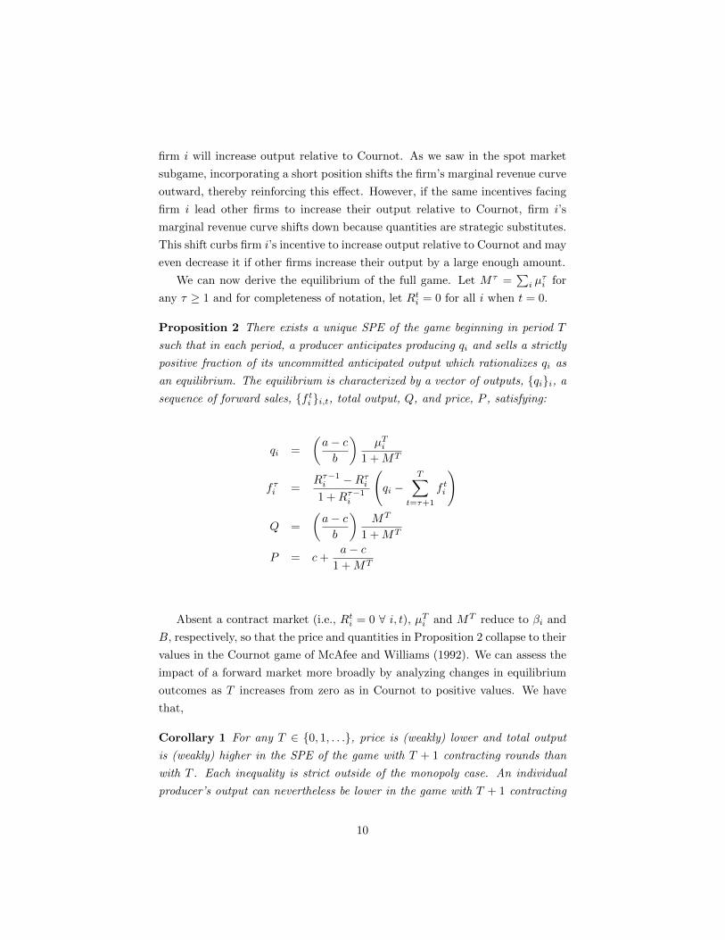
We can now derive the equilibrium of the full game. Let Mτ =∑i µ

τi for

any τ ≥ 1 and for completeness of notation, let Rti = 0 for all i when t = 0.

Proposition 2 There exists a unique SPE of the game beginning in period T

such that in each period, a producer anticipates producing qi and sells a strictly

positive fraction of its uncommitted anticipated output which rationalizes qi as

an equilibrium. The equilibrium is characterized by a vector of outputs, {qi}i, a

sequence of forward sales, {f ti }i,t, total output, Q, and price, P , satisfying:

qi =

(a− cb

)µTi

1 +MT

fτi =Rτ−1i −Rτi1 +Rτ−1i

(qi −

T∑t=τ+1

f ti

)

Q =

(a− cb

)MT

1 +MT

P = c+a− c

1 +MT

Absent a contract market (i.e., Rti = 0 ∀ i, t), µTi and MT reduce to βi and

B, respectively, so that the price and quantities in Proposition 2 collapse to their

values in the Cournot game of McAfee and Williams (1992). We can assess the

impact of a forward market more broadly by analyzing changes in equilibrium

outcomes as T increases from zero as in Cournot to positive values. We have

that,

Corollary 1 For any T ∈ {0, 1, . . .}, price is (weakly) lower and total output

is (weakly) higher in the SPE of the game with T + 1 contracting rounds than

with T . Each inequality is strict outside of the monopoly case. An individual

producer’s output can nevertheless be lower in the game with T + 1 contracting

10

rounds relative to T if its capital stock is sufficiently small relative to that of its

competitors.

Allaz and Vila (1993) provide a special case of this result for a symmetric

two-firm oligopoly. When firms are symmetric, our model shows that all firms

increase their output as T increases, as they do in Allaz and Vila (1993). Corol-

lary 1 shows that this may no longer be the case when firms are asymmetric.

This result suggests that the introduction of a forward market may increase

concentration as measured by output, even as it improves welfare.

The impact of the forward market on output can be substantial. Consider

the special case of constant marginal cost (e = 0) and a single contracting stage

(T = 1). In this case, βi = 1 so that hi = N−1N , µ1

i = N , and M1 = N2. The

presence of a forward market increases output by 140 percent when N = 2 and

by nearly 600 percent when N = 6. These increases would be somewhat smaller

if marginal costs were instead increasing (e = 1) and larger with multiple rounds

of contracting (T > 1).

3 Market Structure and Welfare

We now examine the role of market structure in evaluating the impact of a for-

ward market on welfare. Whereas Allaz and Vila (1993) showed that welfare can

span duopoly-Cournot to perfect competition levels as the number of contract-

ing rounds increases, our focus is on how the welfare impact of a forward market

is influenced by market structure. As such, we treat T as fixed, determined by

the particulars of the industry.5

3.1 Market structure and hedge rates

The welfare impact of a forward market is related to the fraction of each firm’s

output that is contracted in the forward market, i.e. its “hedge rate.” The

following result aids the understanding of this relationship.

Lemma 2 Given equilibrium strategies within the SPE of the (T + 1)-stage

game, the hedge rate can be expressed as hi ≡ q0iqi

= |RTi | =MT−i

1+MT−i

.

The result is fairly general in that the first equality, hi = |RTi |, does not

rely on the shape of the demand or cost functions. It follows from the fact

5Bushnell (2007) discusses the institutional details of forward sales within wholesale elec-tricity.

11

that a firm, when deciding how much to supply on the contract market, takes

into account that a marginal increase in supply will be met by a decrease in its

competitors’ sales in subsequent periods. Thus, while a marginal increase in con-

tracted supply on its own causes the price to decline, the corresponding decrease

in competitors’ outputs partially offsets this. The optimum equates marginal

revenue across each of T + 1 stages much in the way that a third-degree price

discriminating monopolist equates marginal revenue across customer segments.

A firm’s hedge rate depends at a first order on the amount of capital stock

controlled by its competitors as well as the distribution of capital stock among

them.6 Competitors with larger capital stocks produce more irrespective of

hedging, so their response to firm i’s contracted quantity will be larger. At the

same time, because larger firms make less efficient use of their capital stocks,

firm i’s hedge rate is larger when the capital stocks of its competitors are more

symmetrically distributed.7 The upshot is that the structural conditions which

lead a firm to sell a larger fraction of its output in the contract market are the

same conditions that lead to greater output in the baseline Cournot model.

As a further illustration, consider the perfectly symmetric case (i.e., βi = β

for all i). The (common) hedge rate when T = 1 is,

h(1) =(N − 1)β

1 + (N − 1)β. (3)

That h(1) is larger for larger values of N suggests that from a welfare perspec-

tive, a forward market is not a perfect substitute for a competitive industry

structure because forward contracting is more prevalent when the industry is

more competitive. This interpretation continues to hold for larger values of T .

To see this, we have from Lemmas 1 and 2 that the hedge rate when T = 2 is,

h(2) = H(h(1)

)≡ (N − 1)β

1 +(N − 1− h(1)

)β. (4)

Since H is monotonically increasing in h(1) and larger for larger values of N , it

follows that iteration T − 1, h(T ) = HT−1 (h(1)) (where the superscript T − 1

6In the game with T = 1 contracting stages, a firm’s hedge rate, hi = B−i/(1 + B−i),depends only on the capital stocks of its competitors. But when T > 1, the hedge rate dependson µT−i, each of which depends on firm i’s capital stock through its influence on every otherfirm’s hedge rate. The effect of βi on h−i is of a second-order magnitude, however.

7Each βi is concave in capital due to increasing marginal costs. Thus, firms with largercapital stocks produce less per unit of capital than smaller firms. Note that if marginal costsare constant (d = 0) then βi = 1 ∀i.

12

reflects the number of iterations), is also larger for larger values of N . Note that

in the case of monopoly (N = 1), the hedge rate is zero for any T as forward

contracting has no strategic impact.

3.2 Hedge rates and welfare

In Proposition 1, we saw that total output is increasing in F 0, a weighted-

average of forward positions. Lemma 2 showed that a firm’s contracted output

is increasing in its hedge rate, which itself is a function of market structure.

In particular, when the market structure is more competitive—e.g., there are

more firms or capital is distributed more symmetrically among a given number

of firms—hedge rates are higher. This suggests that a forward market creates

an additional channel through which market structure affects welfare.

To formalize this point, we first consider the industry-average Lerner In-

dex, which summarizes the degree to which market output diverges from per-

fect competition and hence is useful as a proxy for consumer and total sur-

plus (Shapiro (1989)). Let si = qi/Q denote firm i’s market share and let

ε = − (∂Q/∂P ) (P/Q) denote the absolute price elasticity of demand.

Lemma 3 Given a vector of hedge rates h, the Lerner Index derived from firms

optimizing subject to h equals

LI (h) ≡∑i

(P − C ′iP

)si =

∑i

s2iε

(1− hi)

Lemma 3 shows that each firm’s price-cost margin percentage is a product of

two terms, the typical Cournot term, s2i /ε, and a term reflecting the importance

of forward contracting, (1− hi). The LI can be evaluated at the SPE hedge

rates, but it also holds for an arbitrary vector of hedge rates, keeping in mind

that si and ε are themselves functions of the hedge rates. As hedge rates increase

uniformly from zero to unity, price-cost margins and hence consumer and total

surplus, span the Cournot outcome at one extreme and perfect competition

at the other. Again holding T fixed, the structural conditions that give rise to

larger hedge rates are the same conditions that give rise to competitive outcomes

in the absence of forward contracting.8

8When T becomes large, hedge rates approach unity and outcomes become competitiveeven under industry structures that look very non-competitive. Allaz and Vila (1993) showedthat, in a symmetric duopoly, as T → ∞, output approaches the perfectly competitive level.

13

3.3 Concentration and welfare

The results already established are sufficient to determine that forward mar-

kets have the greatest impact on outcomes in markets characterized by some

intermediate level of competition/concentration. The (T + 1)-stage model is

equivalent to the baseline model of Cournot competition in the monopoly case

(Corollary 1), and both models converge to perfect competition as market shares

approach zero (Lemma 3). Thus, if forward markets lower price and increase

output (Corollary 1) then the magnitude of these effects must be maximized in

markets with firms that have market shares bounded strictly by zero and unity.

We present the result using both consumer surplus (CS) and total surplus

(TS) as measures of welfare. These can be expressed as functions of total output

and the average price-cost margin:9

CS =b

2Q2

TS =Q

2

[a− c+

∑i

si

(P − C

′

i

)](5)

Let ρCS denote the ratio of consumer surplus in the SPE of (T + 1)-stage model

to consumer surplus in Cournot, holding constant all model parameters. Let

ρTS denote the analogous ratio with respect to total surplus.

Next, we define what it means for concentration to decrease from monopoly

at one extreme to the limiting case of perfect competition. Assume that there

is an infinite number of potential producers, but that at any time, there are

only a finite number whose capital stocks are strictly positive. We will then

consider transfers of capital among a subset of potential producers, N, that

reduces the absolute difference in capital between every producer in N. Suppose

that a transfer changes the capital allocation from k to k′ where ki and k′i are

elements of k and and k′, respectively. Following Waehrer and Perry (2003), an

equalizing transfer is such that: (i) |ki − kj | >∣∣k′i − k′j∣∣ for every i, j ∈ N; (ii)∑

i∈N ki =∑i∈N k′i; and (iii) kl = k′l for all l /∈ N. With respect to mergers, the

pre-merger allocation of capital can be recovered from the post-merger allocation

via an equalizing transfer.

We model perfect competition as the limiting case, of all allocations in which

all firms with positive capital stocks are symmetric, as the number of such firms

goes to infinity. A symmetric equalizing transfer is an equalizing transfer moving

9Derivations are in the Appendix.

14

from k to k′ in which: i) k′i = k′j for every i, j ∈ N ; and ii) k′i < ki for every

i, j ∈ N . The industry approaches perfect competition from any arbitrary initial

allocation of capital through a sequence of symmetric equalizing transfers.

Proposition 3 If k is the monopoly allocation, then any equalizing transfer

from k increases ρCS and ρTS. For any allocation k other than the monopoly

allocation, there exists an allocation k, such that any symmetric equalizing trans-

fer to k causes ρCS and ρTS to decline.

Proposition 3 is one of our core results. The idea is that when markets are suf-

ficiently concentrated, a small decrease in concentration increases welfare more

in the presence of a forward market. A large enough decrease in concentration

from an intermediate allocation can increase welfare relatively more in the ab-

sence of a forward market. In the remainder of this section, we use numerical

techniques to illustrate how forward markets have the greatest impact on welfare

with intermediate levels of competition/concentration.

We first compare the welfare statistics obtained with T = 1 rounds of forward

contracting to those obtained in Cournot equilibrium (T = 0). To do so, we

create data on 9,500 “industries,” evenly split between N = 1, 2, . . . , 20. For

each industry, we calibrate the structural parameters of the model (a, b, c,

k) such that Cournot equilibrium exactly matches randomly-allocated market

shares, an average margin, and normalizations on price and total output.10 We

then obtain the welfare statistics that arise in Cournot equilibrium and with a

single round of forward contracting.

Figure 1 summarizes the results. In each panel, the vertical axis provides the

ratio of surplus with forward contracting to surplus with Cournot. The horizon-

tal axes shows the Herfindahl-Hirschman index (“HHI”). The HHI is the sum

of squared market shares, which attains a maximum of unity in the monopoly

extreme and asymptotically approaches zero as the market approaches perfect

competition. The HHI is an appealing statistic due to its well-known theoretical

connection to welfare in the baseline Cournot model; it also features prominently

in the Merger Guidelines of the U.S. Department of Justice and Federal Trade

Commission.11 In the graphs, each dot represents a single industry, and the

lines provide nonparametric fits of the data.

As shown, consumer surplus and total surplus are greater with forward con-

tracting than with Cournot (because all dots exceed unity). Further, consistent

10We normalize P = Q = 100 and use an average margin of 0.40.11Notice that when all hi = 0, LI = HHI/ε.

15

1

1.05

1.1

1.15

1.2

1.25

1.3

Perfo

rman

ce R

elat

ive

to C

ourn

ot

0 .1 .2 .3 .4 .5 .6 .7 .8 .9 1HHI

Consumer Surplus

.4

.5

.6

.7

.8

.9

1

0 .1 .2 .3 .4 .5 .6 .7 .8 .9 1HHI

Producer Surplus

1

1.01

1.02

1.03

1.04

1.05

1.06

0 .1 .2 .3 .4 .5 .6 .7 .8 .9 1HHI

Total Surplus

Figure 1: Welfare Statistics with Heterogeneous Capital Stocks

with Corollary 1, the impact of a forward market is greatest at intermediate

levels of competition.12 The gain in consumer surplus is maximized at an HHI

around 0.30, which corresponds roughly to a symmetric three firm oligopoly.

The gain in total surplus is maximized at an HHI around 0.40, between the

symmetric triopoly and duopoly levels. The figure also shows that forward

markets diminish producer surplus, particularly in non-concentrated markets.

It is also possible to compare the welfare statistics that arise with forward

contracts to those obtained with perfect competition. This is especially tractable

in the special case of symmetric firms and constant marginal costs (e = 0). The

12As there is not a one-to-one correspondence between HHI and consumer or total surplus,we view these results as illustrative. The advantage to using HHI to measure concentrationis that it offers a complete ordering of any two capital allocations and hence allows us toplot the results. In the following section, we analyze a more theoretically-robust measure ofconcentration that does not offer a complete concentration-ordering of allocations.

16

expressions in (5) can be presented as functions of the common hedge rate:

CS(h(T )) =(a− c)2

2

(N

N + 1− h(T )

)2

TS(h(T )) =(a− c)2

2

(N

N + 1− h(T )− 1

2

(N

N + 1− h(T )

)2)

The analogous expressions with perfect competition are CS(1) = TS(1) =12 (a− c)2. Thus, the levels of consumer surplus and of total surplus with for-

ward contracts, relative to perfect competition, are free of the demand and cost

parameters and depend only on the number of firms and the hedge rate. This

holds for any given hedge rate, including the SPE rates h(T ).

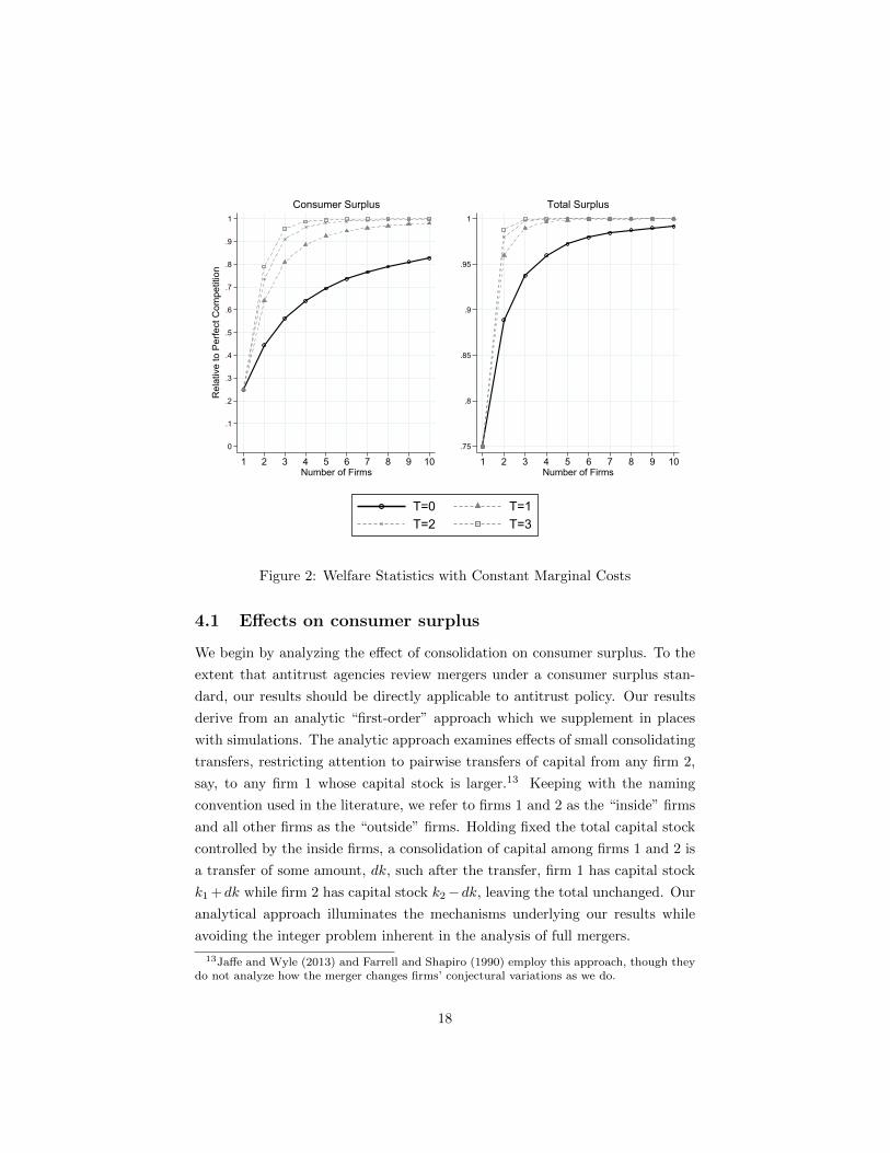
Figure 2 plots the ratios CS(h(T ))/CS(1) andW (h(T ))/W (1) for T = 0, . . . , 3.

Again, T = 0 corresponds to Cournot competition and h(0) = 0. The horizontal

axis in each panel is the number of firms (N = 1, ..., 10) which, under symmetry,

is a sufficient statistic for concentration. As shown, consumer surplus and total

surplus increase with N under Cournot equilibrium; in the limit as N → ∞these welfare statistics approach the perfectly competitive level. Incorporating

each round of contracting adds curvature to the relationship between surplus

and the number of firms, such that surplus approaches the perfectly competi-

tive level faster as N grows large. The “gap” between surplus with Cournot and

surplus with forward contracts is largest for intermediate N , again consistent

with Proposition 3. Lastly, the figure is highly suggestive that forward mar-

kets amplify the impacts of market structure changes (e.g., mergers) on welfare

in concentrated markets, but diminish impacts otherwise. We provide a more

sophisticated analytical treatment of capital transfers in the next section.

4 Mergers

In this section, we analyze the welfare impacts of consolidation, which we treat

as the transfer of capital stock from small to large firms. Mergers are inherently

consolidating regardless of whether the larger or smaller firm is the acquirer

because the merged firm’s capital stock will be larger than either of the merging

firms’. Our interest extends beyond mergers to partial acquisitions as many real-

world applications involve the sale of individual plants. Even when evaluating

full mergers, antitrust authorities must often consider whether and to what

extent a partial divestiture might offset the anticompetitive harm.

17

0

.1

.2

.3

.4

.5

.6

.7

.8

.9

1R

elat

ive

to P

erfe

ct C

ompe

titio

n

1 2 3 4 5 6 7 8 9 10Number of Firms

Consumer Surplus

.75

.8

.85

.9

.95

1

1 2 3 4 5 6 7 8 9 10Number of Firms

Total Surplus

T=0 T=1T=2 T=3

Figure 2: Welfare Statistics with Constant Marginal Costs

4.1 Effects on consumer surplus

We begin by analyzing the effect of consolidation on consumer surplus. To the

extent that antitrust agencies review mergers under a consumer surplus stan-

dard, our results should be directly applicable to antitrust policy. Our results

derive from an analytic “first-order” approach which we supplement in places

with simulations. The analytic approach examines effects of small consolidating

transfers, restricting attention to pairwise transfers of capital from any firm 2,

say, to any firm 1 whose capital stock is larger.13 Keeping with the naming

convention used in the literature, we refer to firms 1 and 2 as the “inside” firms

and all other firms as the “outside” firms. Holding fixed the total capital stock

controlled by the inside firms, a consolidation of capital among firms 1 and 2 is

a transfer of some amount, dk, such after the transfer, firm 1 has capital stock

k1 +dk while firm 2 has capital stock k2−dk, leaving the total unchanged. Our

analytical approach illuminates the mechanisms underlying our results while

avoiding the integer problem inherent in the analysis of full mergers.

13Jaffe and Wyle (2013) and Farrell and Shapiro (1990) employ this approach, though theydo not analyze how the merger changes firms’ conjectural variations as we do.

18

Extrapolating to larger transfers such as full mergers involves integrating

over these first-order effects. When first-order effects are insufficient to evaluate

larger transfers or otherwise are aided by additional illustration, we provide

simulations of full mergers. We restrict attention to a single round of forward

contracting (T = 1) to simplify the mathematics, and remove the corresponding

superscripts as appropriate. Because consumer surplus is increasing in total

output (from (5)), any transfer of capital that reduces the equilibrium output

reduces consumer surplus. Formally, the change in consumer surplus due to a

consolidating transfer of capital is,

dCS = b · dQ =a− c

(1 +M)2

∑i

dµi.

We can deconstruct the output effect into two components, a structural effect

(SE), which measures the change in output holding each firm’s hedge rate fixed,

and a hedging effect (HE), which measures the incremental change in output

due to changes in how the new structure changes firms’ conjectural variations.

Keeping in mind that µi = βi1+βiRi

(Lemma 1), we have that,

dµi =

(µiβi

)2dβi − µ2

i · dRi if i = 1, 2

−µ2i · dRi if i 6= 1, 2

Collecting the dβi terms and the dRi terms, respectively, the change in consumer

surplus is, dCS = SE +HE, where,

SE ≡ a− c(1 +M)

2

[(µ1

β1

)2

dβ1 +

(µ2

β2

)2

dβ2

]< 0

HE ≡ − a− c(1 +M)

2

∑i

µ2i · dRi < 0

This deconstruction allows us to state the following proposition.

Proposition 4 All consolidating transfers reduce consumer surplus in the pres-

ence of a forward market. The loss of consumer surplus due to a consolidating

transfer is mitigated if each firm’s hedge rate remains fixed at its pre-transfer

value.

That consolidation leads to lower output should not be surprising as the

result holds within the baseline model of Cournot competition. What it inter-

19

esting is that the reduction is output is magnified when firms adjust their hedge

rates in response to consolidation as they do in the SPE of the two-stage game.

This follows from the fact that SE,HE < 0. The strategic effect is negative for

the standard reasons: The capital transfer leads the inside firms to reduce out-

put, while outside firms react by expanding their output. The total expansion

across all outside firms only partially offsets the output reduction by the inside

firms, leading to a net decrease in industry output.14 The hedging effect is neg-

ative due to how the capital transfer affects firms’ conjectures about competitor

responses to a change in their contracted quantity. Outside firms anticipate that

the inside firms will be less responsive to their contracted quantities on the basis

that the inside firms produce less overall. At the same time, the inside firms

have less incentive to contract since there is less productive capacity outside

their control. This reduces the amount of forward contracting in equilibrium

and thereby weakens a constraint on the exercise of market power.

It is natural to ask whether the effect of consolidation is more pronounced

within the two-stage game relative to the baseline Cournot game.

Proposition 5 There exists a capital allocation k such that the reduction in

consumer surplus due to consolidation is greater within the SPE of the two-

stage model than in Cournot. There exists a capital allocation k′ that is less

concentrated than k under the transfer principle such that the reduction in con-

sumer surplus due to consolidation is greater in Cournot than in the SPE of the

two-stage model.

Proposition 5 says that the welfare effects of consolidating transfers within

the two-stage model are greater than Cournot in industries that are sufficiently

concentrated and smaller than Cournot in industries that are unconcentrated.

The reason why contracting doesn’t always lead to a greater reduction in con-

sumer surplus is that consumer surplus depends on the pre-transaction hedge

rate. Within the two-stage model, the effect of a change in structure on each

firm’s output is proportional to its pre-transaction output. As a result, the

structural effect is damped relative to Cournot, substantially so when the in-

dustry is fairly unconcentrated. Recall from Section 3.1 that hedge rates decline

in concentration. It follows that as the capital stock becomes more concentrated,

hedge rates decline and each firm’s output in the two-stage game converges to

its output in the Cournot game. Proposition 5 establishes what amounts to

14See Farrell and Shapiro (1990) for this result in Cournot oligopoly.

20

a threshold level of concentration where the hedging effect exactly offsets the

greater structural effect within Cournot.

We revisit the Monte Carlo experiments to illustrate and extend the analyses

beyond first-order effects to full mergers.15 We create data on 9,000 industries

evenly split between N = 2, 3, . . . , 20, and calibrate the structural parameters

of the model to match randomly-allocated market shares, an average margin

of 0.40, and normalizations on price and total output. We then simulate eco-

nomic outcomes using the obtained structural parameters under the alternative

assumption of Cournot competition (T = 0). Finally, to simulate mergers, we

combine the capital stocks of the first and second firm of each industry and

recompute equilibria both with the two-stage model and with Cournot.

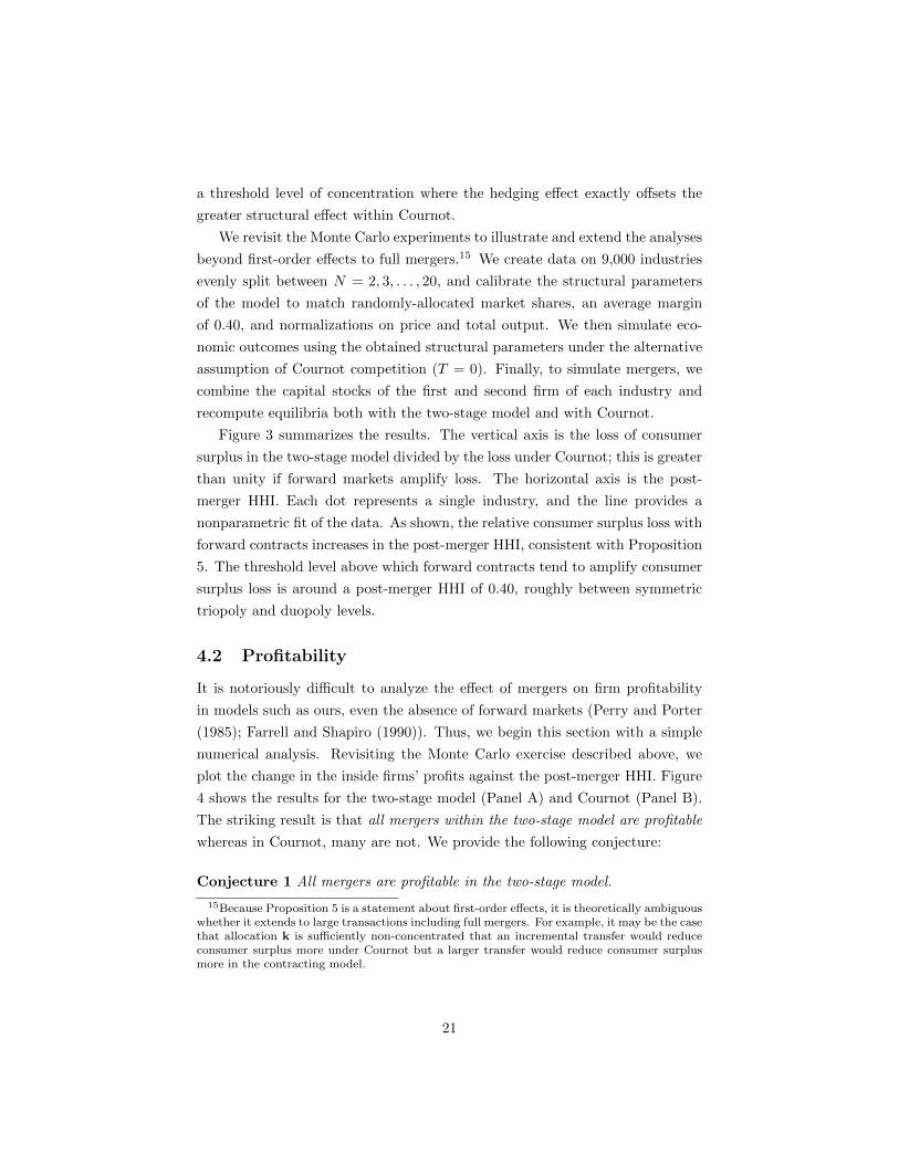
Figure 3 summarizes the results. The vertical axis is the loss of consumer

surplus in the two-stage model divided by the loss under Cournot; this is greater

than unity if forward markets amplify loss. The horizontal axis is the post-

merger HHI. Each dot represents a single industry, and the line provides a

nonparametric fit of the data. As shown, the relative consumer surplus loss with

forward contracts increases in the post-merger HHI, consistent with Proposition

5. The threshold level above which forward contracts tend to amplify consumer

surplus loss is around a post-merger HHI of 0.40, roughly between symmetric

triopoly and duopoly levels.

4.2 Profitability

It is notoriously difficult to analyze the effect of mergers on firm profitability

in models such as ours, even the absence of forward markets (Perry and Porter

(1985); Farrell and Shapiro (1990)). Thus, we begin this section with a simple

numerical analysis. Revisiting the Monte Carlo exercise described above, we

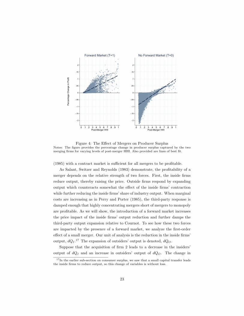
plot the change in the inside firms’ profits against the post-merger HHI. Figure

4 shows the results for the two-stage model (Panel A) and Cournot (Panel B).

The striking result is that all mergers within the two-stage model are profitable

whereas in Cournot, many are not. We provide the following conjecture:

Conjecture 1 All mergers are profitable in the two-stage model.

15Because Proposition 5 is a statement about first-order effects, it is theoretically ambiguouswhether it extends to large transactions including full mergers. For example, it may be the casethat allocation k is sufficiently non-concentrated that an incremental transfer would reduceconsumer surplus more under Cournot but a larger transfer would reduce consumer surplusmore in the contracting model.

21

0

.5

1

1.5

2

Con

sum

er S

urpl

us L

oss

Rel

ativ

e to

Cou

rnot

0 .1 .2 .3 .4 .5 .6 .7 .8 .9 1Post-Merger HHI

Figure 3: Relative Consumer Surplus Loss with Forward MarketsNotes: The vertical axis provides the percentage change in consumer surplus with forwardmarkets divided by the percentage change without forward markets, given the same param-eterization. Values above unity represent the effects of mergers for which forward marketsamplify consumer surplus loss. The horizontal axis provides the post-merger HHI. The lineprovides a nonparametric fit of the data.

This may help offer a more complete response to the “merger paradox.”

Salant, Switzer and Reynolds (1983) examined the incentive to merge within a

symmetric model of Cournot competition with constant marginal cost. They

find that pairwise mergers are not profitable unless they form a monopoly. It

is difficult to explain the prevalence of mergers in light of this result, hence

the paradox.16 Perry and Porter (1985) argue that the failure to explain the

profitability of mergers is actually a misconception since the mergers are not

well-defined conceptually when firms can produce seemingly infinite quantities

at a constant marginal cost. They propose a model of capital stocks, the same

model we have adopted, and find that smaller mergers can indeed be profitable

even when firms compete on quantities. Yet many mergers within their frame-

work are unprofitable. Figure 4 suggests that supplementing Perry and Porter

16Deneckere and Davidson (1985) alter the assumption that firms compete on quantity andshow that mergers are always profitable when firms offer differentiated products and competeon price. The conflicting result arises because prices are strategic complements. In that case,an increase in the inside firms’ prices is met by an increase in the prices of outside firms,hence mergers are profitable. But the assumption that products are differentiated may notbe applicable in many settings such as the sale of commodities or wholesale electricity.

22

-.2

-.15

-.1

-.05

0

.05

.1

.15

.2Pe

rcen

tage

Cha

nge

in P

rofit

0 .1 .2 .3 .4 .5 .6 .7 .8 .9 1Post-Merger HHI

Forward Market (T=1)

-.2

-.15

-.1

-.05

0

.05

.1

.15

.2

0 .1 .2 .3 .4 .5 .6 .7 .8 .9 1Post-Merger HHI

No Forward Market (T=0)

Figure 4: The Effect of Mergers on Producer SurplusNotes: The figure provides the percentage change in producer surplus captured by the twomerging firms for varying levels of post-merger HHI. Also provided are lines of best fit.

(1985) with a contract market is sufficient for all mergers to be profitable.

As Salant, Switzer and Reynolds (1983) demonstrate, the profitability of a

merger depends on the relative strength of two forces. First, the inside firms

reduce output, thereby raising the price. Outside firms respond by expanding

output which counteracts somewhat the effect of the inside firms’ contraction

while further reducing the inside firms’ share of industry output. When marginal

costs are increasing as in Perry and Porter (1985), the third-party response is

damped enough that highly concentrating mergers short of mergers to monopoly

are profitable. As we will show, the introduction of a forward market increases

the price impact of the inside firms’ output reduction and further damps the

third-party output expansion relative to Cournot. To see how these two forces

are impacted by the presence of a forward market, we analyze the first-order

effect of a small merger. Our unit of analysis is the reduction in the inside firms’

output, dQI .17 The expansion of outsiders’ output is denoted, dQO.

Suppose that the acquisition of firm 2 leads to a decrease in the insiders’

output of dQI and an increase in outsiders’ output of dQO. The change in

17In the earlier sub-section on consumer surplus, we saw that a small capital transfer leadsthe inside firms to reduce output, so this change of variables is without loss.

23

insiders’ profits is,

dπI = {[P + (1 +RI)QIP′ − C ′I ] + [dQO/dQI −RI ]QIP ′ + g/dQI}dQI (6)

where: C ′I is the slope of the inside firms’ marginal cost function evaluated at

the pre-merger output; RI is the inside firms’ period-1 conjecture; and g (> 0)

is the cost savings incurred by the inside firms upon rationalizing output across

their combined capital assets. Since dQI < 0, dπI > 0 if and only if the term

in curly brackets is negative. We consider each of its components in turn.

Because insiders reduce their output in equilibrium, it must be the case that

at the pre-merger equilibrium output, its marginal cost exceeds its marginal

revenue. From the inside firms’ period-1 first-order condition, we see that this

is equivalent to [P + (1 +RI)QIP′ − C ′I ] < 0. Since the pre-merger output

puts the insiders on the downward sloping portion of πI with respect to QI , a

small decrease in QI increases profit by − [P + (1 +RI)QIP′ − C ′I ]. Since this

term is decreasing in RI , and since hedge rates decline due to consolidation (an

implication of Proposition 4), it must be that this incremental profit is larger

than it would be if hedge rates were kept constant or were constrained to be

zero in the case of Cournot.

This incremental gain must be weighted against the effect on profit due to

output expansion by outsiders, − [dQO/dQI −RI ]QIP ′. The term inside the

square brackets is the net output response from outsiders due to the merger.

To derive this, consider the solution for firm j’s problem in the contract market

(where we have assumed T = 1),

P (Q) + qj (1 +Rj)P′ (Q) = C ′j (qj) (7)

Differentiating both sides of (7) with respect to Q−j =∑k 6=j qk, we obtain,

dqjdQ−j

≡ rj = − µj1 + µj

(8)

This is the firm’s reaction function ignoring the intertemporal effects of hedging.

From dqj = rjdQ−j , we have that, dqj (1 + rj) = rj (dqj + dQ−j) = rjdQ, or

equivalently,

dqj = −(

rj1 + rj

)dQ = −µjdQ (9)

Summing (9) over all j ∈ O, we have that, dQO = −M−IdQ = −M−I (dQO + dQI),

24

or equivalently,dQ0

dQI= − M−I

1 +M−I(10)

Expression (10) is the gross change in outsiders’ output to a given change in

insiders’ output, irrespective of intertemporal effects of hedging. However, since

some of this response was already internalized by the inside firms pre-merger

via Stackleberg considerations, the net impact of the merger is an expansion of

− [dQO/dQI −RI ].Notice that from (10), −dQO/dQI is equivalent to the inside firms’ hedge

rate in the game with T = 2 rounds of contracting, h(2)I . It follows that the net

output expansion is equal to h(2)I −h

(1)I . In contrast, it is straightforward to show

that the output expansion under Cournot is −BI/ (1 +BI) which is equivalent

to h(1)I . Since hedge rates converge to unity as the number of contracting rounds

increase, we have that h(2)I − h

(1)I < h

(1)I so that it is indeed the case that the

output expansion is damped by forward trading. Furthermore, as the number

of contracting rounds becomes large, the output expansion vanishes entirely.

5 Collusion

We now investigate collusion in the presence of forward markets. We place the

model into a standard repeated-game setting with an infinite number of trading

periods indexed t = 0, 1, 2, . . . . In each period, firms simultaneously sell output

in a spot market and contract for output up to T periods ahead. The discount

factor is δ. Following Liski and Montero (2006), which examines the case of

duopoly, we impose constant marginal costs and hence symmetry in order to

improve the tractability of the incentive compatibility constraints. We advance

the literature primarily by considering an arbitrary number of firms, N .

We focus on a particular set of strategies under which firms collectively pro-

duce the monopoly output, Qm = (a − c)/2, in each period. Let f t,t+τi denote

the quantity contracted by firm i during period t for delivery τ = 1, 2, . . . , T

periods later. Along the collusive path, firms trade in the forward market ac-

cording to f t,t+1i = xQm/N and f t,t+τi = 0 for all τ > 1 and trade in the spot

market according to qsi = (1 − x)Qm/N . We consider x ∈ [−1, 1] so that firms

can be long (x < 0) or short (x > 0) in the spot market. The choice of x feeds

into the incentive compatibility constraints that we develop below. If any firm

deviates from this collusive path, then competition in all subsequent periods re-

verts to the strategies defined by Proposition 2, albeit adjusted in some periods

25

to account for the impact of the deviation on future spot markets.

Because some fraction, x, of sales are already committed in any given period,

the present value of collusion takes the form

V c(δ, x) = (1− x)πm +δ

1− δπm (11)

where πm = (a−c)2/4N is the per-firm monopoly profit. The value of deviation

is more complicated. Suppose the deviation occurs in period t. In the period-t

spot market, firm i (the deviating firm) expands production relative to the collu-

sive level. It also signs forward contracts which allow it to obtain a Stackleberg

leadership position in spot markets in periods t + τ , for τ ∈ {1, 2, . . . , T}. In

the first of these periods, τ = 1, competitors’ contracts are fixed according to

the collusive strategy. Competitors choose their output for the period t+1 spot

market that best respond to firm i’s deviation and to forward positions taken

under the collusive strategy. For spot markets τ ∈ {2, . . . , T} periods ahead,

competitors choose forward quantities in periods t+1 through t+τ−1 as well as

spot quanitities in period t+τ which best respond to firm i’s deviation. In light

of Corollary 1, the punishment is more severe in spot markets further ahead.

For spot markets τ > T periods ahead, firm i obtains no Stackleberg leadership

position and all firms play according to the equilibrium of Proposition 2. Let

πd,τ denote the deviating firm’s profit τ periods post-deviation. We have that,

πd,τ =

πm (N+1−x)2

4N if τ = 0

πm(1− N−1

2N x)2

if τ = 1

πm N1+(N−1)µτ if τ ∈ [2, T ]

πm 4NµT

(1+MT )2if τ > T

(12)

where µτ and MT are as defined in Proposition 2.

We now provide the main theoretical result of the section:

Proposition 6 The aforementioned collusive strategies constitute a SPE if δ ≥δ(x), where for x ∈ [−1, 1], δ(x) solves,

V c(δ, x)

πm=πd,0

πm+ δ

(πd,1

πm

)+

T∑τ=2

δτ(πd,τ

πm

)+δT+1

1− δ

(πd,T+1

πm

)(13)

The demand and cost parameters, a and c, cancel in equation (13) and thus do

26

.3

.4

.5

.6

.7

.8

Crit

ical

Dis

coun

t Rat

e

2 3 4 5 6 7 8 9 10Number of Firms

CournotOptimal Strategies (x=x*)

Figure 5: Effect of Forward Markets on Critical Discount Rates

not affect the critical discount rate.

Of particular interest is how the critical discount rate changes with N . To

make progress, we use numerical techniques to calculate the “optimal” collusive

strategy, x∗(N,T ), that minimizes the critical discount rate as a function of

N and T , and obtain the corresponding critical discount rates. Figure 5 plots

results for the case of T = 1. As one might expect, the critical discount rate

δ(x∗(N, 1)) increases with N , such that collusion becomes more difficult to sus-

tain. For comparison, we also plot the critical discount rate under Cournot,

which also increases with N . It is apparent that (i) forward markets decreases

the critical discount rate relative to Cournot; and (ii) this effect is more pro-

nounced for small N . This suggests that it is more likely that, in the presence

of a forward market, firms will switch from competition to collusion in response

to an increase in concentration. These results are robust to T > 1 in all of

the numerical specifications we have explored: a large T discourages deviation

by making punishment harsher, but encourages deviation by providing a longer

period of Stackleberg leadership. The net effect appears to be small.

The relationship shown in Figure 5 derives from the “hedging effect” identi-

fied in Section 4, whereby consolidation leads firms to reduce forward sales under

the strategies described by Proposition 2, thereby providing an additional boost

to profits. Under Cournot, the critical discount rate decreases in concentration

because greater concentration causes the incremental gain from deviation rel-

ative to cooperation to decline at a greater rate than the incremental gain of

27

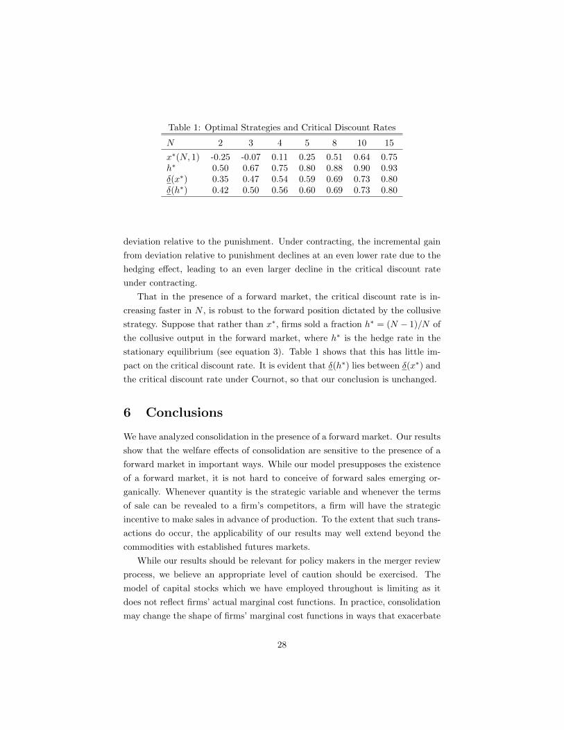
Table 1: Optimal Strategies and Critical Discount Rates

N 2 3 4 5 8 10 15

x∗(N, 1) -0.25 -0.07 0.11 0.25 0.51 0.64 0.75h∗ 0.50 0.67 0.75 0.80 0.88 0.90 0.93δ(x∗) 0.35 0.47 0.54 0.59 0.69 0.73 0.80δ(h∗) 0.42 0.50 0.56 0.60 0.69 0.73 0.80

deviation relative to the punishment. Under contracting, the incremental gain

from deviation relative to punishment declines at an even lower rate due to the

hedging effect, leading to an even larger decline in the critical discount rate

under contracting.

That in the presence of a forward market, the critical discount rate is in-

creasing faster in N , is robust to the forward position dictated by the collusive

strategy. Suppose that rather than x∗, firms sold a fraction h∗ = (N − 1)/N of

the collusive output in the forward market, where h∗ is the hedge rate in the

stationary equilibrium (see equation 3). Table 1 shows that this has little im-

pact on the critical discount rate. It is evident that δ(h∗) lies between δ(x∗) and

the critical discount rate under Cournot, so that our conclusion is unchanged.

6 Conclusions

We have analyzed consolidation in the presence of a forward market. Our results

show that the welfare effects of consolidation are sensitive to the presence of a

forward market in important ways. While our model presupposes the existence

of a forward market, it is not hard to conceive of forward sales emerging or-

ganically. Whenever quantity is the strategic variable and whenever the terms

of sale can be revealed to a firm’s competitors, a firm will have the strategic

incentive to make sales in advance of production. To the extent that such trans-

actions do occur, the applicability of our results may well extend beyond the

commodities with established futures markets.

While our results should be relevant for policy makers in the merger review

process, we believe an appropriate level of caution should be exercised. The

model of capital stocks which we have employed throughout is limiting as it

does not reflect firms’ actual marginal cost functions. In practice, consolidation

may change the shape of firms’ marginal cost functions in ways that exacerbate

28

or mitigate harm from mergers.

We have also assumed the strategic variable to be quantity. In wholesale

electricity markets, spot prices are determined based on price-quantity sched-

ules submitted by firms. In the supply-function equilibrium model of Klemperer

and Meyer (1989), supply functions can be strategic substitutes or complements.

Mahenc and Salanie (2004) study strategic complements in the context of dif-

ferentiated Bertrand spot market competition and find that forward contracting

increases spot market prices. We are aware of no studies that analyze the effect

of mergers within this context. If consolidation lessens the incentive to contract

in advance, then harm from consolidation is mitigated relative to our results.

Finally, we have assumed that all agents have perfect foresight so that the

only motive for firms to sell in the contract market is to influence spot market

competition. As we do not believe this to be the case in practice, our assumption

of perfect foresight was made for the sake of tractability. Allaz (1992) and

Hughes and Kao (1997) show that when foresight is imperfect and firms are risk

averse, equilibrium hedge rates are higher than in the perfect-foresight case.

How hedge rates change in response to a merger in this setting has not been

explored to our knowledge. However, it is conceivable that our basic findings

would still obtain. Consolidation, by increasing market power, increases the

value to the merged firm of withholding output. To the extent that forward

contracting even for the sake of hedging risk comes at the expense of exercising

market power, mergers may well limit the incentive for firms to forward contract.

We leave this issue and the other issues posed in this section to future research.

29

References

Allaz, Blaise, “Oligopoly, Uncertainty and Strategic Forward Transactions,”

International Journal of Industrial Organization, 1992, 10, 297–308.

and Jean-Luc Vila, “Cournot Competition, Forward Markets and Effi-

ciency,” Journal of Economic Theory, 1993, 59, 1–16.

Anderson, Ronald and Mahadevan Sundaresan, “Futures Markets and

Monopoly,” in RW Anderson, ed., The Industrial Organization of Futures

Markets, Lexington: D.C. Heath, 1984, pp. 75–112.

Brown, David P. and Andrew Eckert, “Electricity Market Mergers with

Endogenous Forward Contracting,” 2016. working paper.

Bushnell, James, “Oligopoly Equilibria in Electricity Contract Markets,”

Journal of Regulatory Economics, 2007, 32 (3), 225–245.

, Erin Mansur, and Celeste Saravia, “Vertical Relationships, Market

Structure and Competition: An Analysis of the U.S. Restructured Elec-

tricity Markets,” American Economic Review, 2008, 99 (1), 237–266.

Deneckere, Raymond and Carl Davidson, “Incentives to Form Coalitions

with Bertrand Competition,” The RAND Journal of Economics, 1985, 16

(4), 473–486.

Eldor, Rafael and Itzhak Zilcha, “Oligopoly, Uncertain Demand, and For-

ward Markets,” Journal of Economics and Business, 1990, 42 (1), 17–26.

Farrell, Joseph and Carl Shapiro, “Horizontal Mergers: An Equilibrium

Analysis,” American Economic Review, 1990, 80 (1), 107–126.

Ferreira, Jose Louis, “Strategic Interaction Between Futures and Spot Mar-

kets,” Journal of Economic Theory, 2003, 108, 141–151.

, “The Role of Observability in Futures Markets,” Topics in Theoretical

Economics, 2006, 6 (1). Article 7.

Green, Richard, “The Electricity Contract Market in England and Wales,”

Journal of Industrial Economics, 1999, 47 (1), 107–124.

Hortacsu, Ali and Steven Puller, “Understanding Strategic Bidding in

Multi-Unit Auctions: A Case Study of the Texas Electricity Spot Mar-

ket,” RAND Journal of Economics, 2008, 39 (1), 86–114.

30

Hughes, John S. and Jennifer L. Kao, “Strategic Forward Contracting and

Observability,” International Journal of Industrial Organization, 1997, 16,

121–133.

Jaffe, Sonia and E. Glen Wyle, “The First-Order Approach to Merger

Analysis,” American Economic Journal: Microeconomics, 2013, 5 (4), 188–

218.

Klemperer, Paul D. and Margaret A. Meyer, “Supply Function Equilibria

in Oligopoly under Uncertainty,” Econometrica, 1989, 57 (6), 1243–1277.

Liski, Matti and Juan-Pablo Montero, “Forward Trading and Collusion in

Oligopoly,” Journal of Economic Theory, 2006, 131 (1), 212 – 230.

Mahenc, P. and F. Salanie, “Softening Competition Through Forward Trad-

ing,” Journal of Economic Theory, 2004, 116, 282–293.

McAfee, R. Preston and Michael A. Williams, “Horizontal Mergers and

Antitrust Policy,” The Journal of Industrial Economics, 1992, 40 (2), 181–

187.

Perry, Martin K. and Robert H. Porter, “Oligopoly and the Incentive for

Horizontal Merger,” American Economic Review, 1985, 75 (1), 219–227.

Salant, Stephen W., Sheldon Switzer, and Robert J. Reynolds, “Losses

from Horizontal Merger: The Effects of an Exogenous Change in Industry

Structure on Cournot-Nash Equilibrium,” Quarterly Journal of Economics,

1983, 98, 185–200.

Shapiro, Carl, “Theories of Oligopoly Behavior,” in R. Schmalensee and

R. Willig, eds., Handbook of Industrial Organization vol 1, New York: El-

sevier Science Publishers, 1989, chapter 6, pp. 330–414.

Sweeting, Andrew and Xuezhen Tao, “Dynamic Oligopoly Pricing with

Asymmetric Information: Implications for Mergers,” 2016. working paper.

Waehrer, Keith and Martin K. Perry, “The Effects of Mergers in Open

Auction Markets,” RAND Journal of Economics, 2003, 34 (2), 287–304.

Wolak, Frank, “An Empirical Analysis of the Impact of Hedge Contracts

on Bidding Behavior in a Competitive Electricity Market,” International

Economic Journal, 2000, 14 (2), 1–39.

31

Appendices

A Proofs

A.1 Proof of Proposition 1

Fixing the price at a candidate equilibrium value, P , and using the definitionof βi given in the text, we can express equation (1) as,

qi =

(ki

bki + d

)(P − c) +

(bki

bki + d

)q0i

=βib

(P − c) + βiq0i

Using the definitions of B and F 0 from the text, we can express total outputas,

Q =∑i

qi =B

b(P − c) + F 0

Substituting the identity Q = (a− P ) /b into the left-hand side of the aboveexpression yields

a− Pb

=B

b(P − c) + F 0

It is straightforward to solve the above for the equilibrium value of P , which wethen plug into the above expressions for qi and Q to obtain their equilibriumvalues.

A.2 Proof of Lemma 1

Consider t = 1. From the expression of qi in Proposition 1, we have that,

∂qi∂f1i

=βi (1 +B−i)

1 +B. (A.1)

From the same expression of qi, we also have that,

∂qj∂f1i

= − βiβj1 +B

.

so that ∑j 6=i

∂qj∂f1i

= −βiB−i1 +B

. (A.2)

Using (A.1) and (A.2), we have that,

R1i ≡

∑j 6=i

∂qj∂f1i

/∂qi∂f1i

= − B−i1 +B−i

32

Now consider any t = τ > 1. Fixing price at some candidate equilibrium, P ,and using the definition of µτi from the statement of the lemma, we can expressequation (2) as,

qi = µτi

(P − cb

)+ µτi (1 +Rτi ) qτi (A.3)

Define the following terms:

F τ =∑i

µτi (1 +Rτi ) qτi , Fτ−i =

∑j 6=i

µτj(1 +Rτj

)qτj

We can then express total output as,

Q =∑i

qi = Mτ

(P − cb

)+ F τ (A.4)

Substituting Q = (a− P ) /b into the above yields,

a− Pb

= Mτ

(P − cb

)+ F τ (A.5)

It is straightforward to solve the above expression for the equilibrium value ofP , which we then plug into (A.3) to obtain,

qi (qτ ) =

(a− cb

)µτi

1 +Mτ+

µτi1 +Mτ

[(1 +Mτ

−i)

(1 +Rτi ) qτi − F τ−i]

(A.6)

Differentiating qi (qτ ) with respect to the firm’s own forward position yields,

∂qi (qτ )

∂fτi=µτi (1 +Rτi )

1 +Mτ

(1 +Mτ

−i)

(A.7)

Differentiating with respect to another firm’s position yields,

∂qj (qτ )

∂fτi=µτi (1 +Rτi )

1 +Mτµτ

so that, ∑j 6=i

∂qj (qτ )

∂fτi=µτi (1 +Rτi )

1 +MτMτ−i (A.8)

Using (A.7) and (A.8), we have that,

Rτ+1i ≡

∑j 6=i

∂qj

∂fτ+1i

/∂qi

∂fτ+1i

= −Mτ−i

1 +Mτ−i

33

A.3 Proof of Proposition 2

Set τ = T in equation (A.5). By construction, FT = 0 since T is the first periodin which forward contracts are bought or sold and FT has been defined as toreflect sales that occurred prior to period T . Solving (A.5) for P , we have,

P = c+a− c

1 +MT(A.9)

Set τ = T in equation (A.4), where again, FT = 0 by construction. Substitutingin expression (A.9) for P in equation (A.4), we have,

Q =

(a− cb

)MT

1 +MT

Finally, set τ = T in equation (A.6), whereby qTi = FT−i = 0. We have,

qi =

(a− cb

)µTi

1 +MT(A.10)

We now proceed to characterize the firm’s forward sales. In equilibrium, itmust be that case that for any period τ > 1, qi (qτ ) = qi

(qτ−1

). In other words

period-τ behavior cannot cause firm i to deviate from its strategy; if it did, thenthe strategy was not an equilibrium to begin with. Since the firm’s marginalcost in equation (2) is the same regardless of τ , so too is its marginal revenue.

Equating marginal revenue between periods T − 1 and T , while using thefact that, qTi = 0 and qT−1i = fTi , we have,(

qi − fTi) (

1 +RT−1i

)= qi

(1 +RTi

)It follows that the firm’s contracted quantity in period T is,

fTi =

(RT−1i −RTi1 +RT−1i

)qi,

where qi is the equilibrium value from equation (A.10). It’s uncommitted outputat the beginning of period T − 1 is,

qi − fTi =1 +RTi

1 +RT−1i

(A.11)

Continuing in this manner, we equate marginal revenue between periods T − 1and T − 2, so that,(

qi − fTi − fT−1i

) (1 +RT−1i

)=(qi − fTi

) (1 +RT−1i

)

34

The firm’s contracted quantity in period T − 1 is,

fT−1i =RT−2i −RT−1i

1 +RT−2i

(qi − fTi

),

where qi − fTi is the value from equation (A.11). Continuing in this manner,the expression for the firm’s forward quantities is true by induction.

A.4 Proof of Corollary 1

Let Q(t) denote total output in a game with t rounds of forward contracting.Further, let M (t) ≡ MT when there are t rounds of forward contracting. Tocomplete the notation, suppose that M (0) = B. From Proposition 2, we havethat Q(t) > Q(t−1) if and only if M (t) > M (t−1).

We can construct any MT recursively beginning with R1i as given in Lemma

1. R1i feeds into µ1

i , which feeds into M1−i, which feeds into R2

i and so on.

Claim 1 Outside the monopoly case, R1i ∈ (−1, 0) and Rt+1

i < Rti regardless ofT .

Proof. Outside the monopoly case, B−i > 0 for every i. It is obvious then thatR1i = −B−i/(1 +B−i) ∈ (−1, 0). Suppose by way of induction that Rti > Rt−1i

regardless of the number of contracting rounds in the game. If Rti > Rt−1i , thenµti > µt−1i , which implies M t

−i > M t−1−i . This implies that,

Rt+1i = −

M t−i

1 +M t−i

< −M t−1−i

1 +M t−1−i

= Rti

irrespective of T .RTi > RT−1i implies that µTi > µT−1i . From this we have that, MT > MT−1,

where it is evident that M t = M (t) regardless of the number of contractingrounds in the game. Since output is higher with more round of forward con-tracting, it is mechanically true that price is lower.

In the monopoly case, B−i = 0 for the only producer i with strictly positivecapital stock. It follows that R1

i = 0, which implies µ1i = βi, which implies

M1 = B. Continuing in this manner, it is evident that for any t, M t = M t−1 =· · · = B, so that total output and hence price are invariant to the number ofcontracting rounds.

By Proposition 2, an individual producer’s output is greater with T = 1round of forward contracting if and only if,

µ1i

1 +M1>

βi1 +B

After manipulating terms, this is equivalent to,

βi >1

R1i

(1 +B−i1 +M1

−i− 1

)

35

The right-hand side of the above expression is bounded above zero in all butthe monopoly case. Therefore, when there are at least three firms, the right-hand side remains bounded above zero even as βi → 0. It follows that for βisufficiently close to zero, the condition fails.

A.5 Proof of Lemma 2

It was established in the proof of Proposition 2 that a producer’s marginalrevenue is equal across each period. Equating its period-T marginal revenuewith its period-0 marginal revenue, we have,

qi(1 +RTi

)= qi − q0i

Rearranging terms, we have that,

q0iqi

=∣∣RTi ∣∣

A.6 Proof of Lemma 3

The solution to the producer’s problem in period T is characterized by a mod-ified version of equation (2) in which τ = T and qTi = 0 for all i. Rearrangingterms, we have,

P − C ′iP

= −qiPP ′ (Q)

(1 +RTi

)= −Q

PP ′ (Q) si (1− hi)

=si (1− hi)

ε

where the second line uses the result of Lemma 2 that hi = RTi and uses thesubstitution, qi = siQ. The third line uses the definition of demand elasticity,ε. Pre-multiplying by si then summing over all i obtains the result.

A.7 Derivation of consumer and total surplus

Consumer surplus is social surplus net of expenditures, so that,

CS =

∫ Q

0

(a− bx− P ) dx = (a− P )Q− b

2Q2 =

b

2Q2.

Total surplus is social surplus net of costs, so that,

TS =

∫ Q

0

(a− bx) dx−∑i

Ci = aQ− b

2Q2 −

∑i

Ci (A.12)

36

By construction, Ci = cqi + q2i /2ki, which implies that marginal cost is of the

form, C′

i = c+ qi/ki. It follows that,

∑i

Ci =∑i

qi

[c+

1

2

(C′

i − c)]

=1

2

[(c+ P )Q−

∑i

qi

(P − C

′

i

)]

Substituting qi = Qsi and P = c+ bQ/M (from Proposition 2), we have,

∑i

Ci =Q

2

[2c+

b

MQ−

∑i

si

(P − C

′

i

)](A.13)

Combining (A.12) and (A.13), we have,

TS =Q

2

[2 (a− c)− b (1 +M)

MQ+

∑i

si

(P − C

′

i

)](A.14)

Finally, from Proposition 2, b(1+M)Q/M = a−c. Substituting this into (A.14)yields the desired expression.

A.8 Proof of Proposition 3

The proof relies on the following being true: 1) ρCS = ρTS = 1 in the monopolycase; 2) ρCS > 1 and ρTS > 1 in all allocations of capital other than monopoly;and 3) ρCS → 1 and ρTS → 1 in the limit of an infinite sequence of symmetricequalizing transfers. The first of these has already been shown in Corollary 1.We turn now to the second result.

Because output is higher in the presence of a forward market outside themonopoly case (Corollary 1), so too is consumer surplus (i.e., ρCS > 1). Thesame is not necessarily true with respect to total surplus when firms are asym-metric. There are two cases to consider. If all firms expand output in thepresence of a forward market, then since price exceeds marginal cost, total sur-plus is necessarily higher. Alternatively, if some firms reduce output, Corollary1 showed that only small firms do so. It follows that since total output is higherin the presence of a forward market, the reduction in output by smaller firms ismore than offset by the output expansion of large firms. Since larger firms aremore efficient, total surplus is higher.

The third result derives from (2). Rearranging terms in (2), we have that inperiod T , each firm chooses qi to solve, (P − C ′i)/P = si(1 − hi)/ε. Applyingan infinite sequence of symmetric equalizing transfers, si → 0 so that P = cregardless of hi.

A.9 Proof of Proposition 4

The proof proceeds in two parts, first showing that the structural effect is neg-ative, then showing that the hedging effect is negative. That both effects are

37

negative is sufficient to show that the transfer reduces consumer surplus. Thatthe hedging effect alone is negative is sufficient to say that the reduction inconsumer surplus is mitigated absent the hedging effect.

Lemma 4 SE ≡ a−c(1+M)2

[(µ1

β1

)2dβ1 +

(µ2

β2

)2dβ2

]≤ 0

Proof. Using,

dβ1 = be

(β1bk1

)2

dk (A.15)

and,

dβ2 = −be(β2bk2

)2

dk = −(β2bk2

)2(β1bk1

)−2dβ1 (A.16)

SE can be expressed as,

SE =a− c

(1 +M)2

[(µ1

β1

)2

−(µ2

β2

)2(β2bk2

)2(β1bk1

)−2]dβ1

Since dβ1 > 0, it is sufficient to show that the square-bracketed term is nonpos-itive. This reduces to, (

µ1

bk1

)2

−(µ2

bk2

)2

≤ 0

Using difference-of-squares (i.e. x2 − y2 = (x+ y) (x− y)), it is sufficient that

µ1

bk1− µ2

bk2≤ 0,

or equivalently,µ1k2 − µ2k1 ≤ 0

By construction, k1 ≥ k2. We can define δ ≥ 0 such that k2 ≡ k1 − δ. Theabove inequality simplifies to,

(µ1 − µ2) k1 − µ1δ ≤ 0 (A.17)

Using the identity,

µi =βi

1 + βiRi=

βi (1 +B − βi)(1 +B) (1− βi) + β2

i

(A.18)

we have that,

(µ1 − µ2) k1 =(1 +B) (1 +B − β1 − β2) (β1 − β2) k1

[(1 +B) (1− β1) + β21 ] [(1 +B) (1− β2) + β2

2 ]

=(1 +B) (1 +B − β1 − β2)β1 (1− β2) δ

[(1 +B) (1− β1) + β21 ] [(1 +B) (1− β2) + β2

2 ]

38

If δ = 0, then condition (A.17) holds trivially. If δ > 0, condition (A.17) reducesto, 1 +B > β1, which is true by construction.

Lemma 5 HE ≡ − a−c(1+M)2

∑i µ

2i dRi ≤ 0

Proof. We have that,

dRi = − dB−i

(1 +B−i)2 ,

where,

dB−i =

dβ2 if i = 1

dβ1 if i = 2

dβ1 + dβ2 if i > 2

It follows that,

HE

(a− c

(1 +M)2

)−1= [dβ1 + dβ2]

∑j 6=1,2

(µj

1 +B−j

)2

+

[(µ1

1 +B−1

)2

dβ2 +

(µ2

1 +B−2

)2

dβ1

]

It suffices to show that each of the square-bracketed terms are negative. Fromequations (A.15) and (A.16) we have that,

dβ1 + dβ2 =

[1−

(β2bk2

)2(β1bk1

)−2]dβ1

=

[(β1bk1

)2

−(β2bk2

)2](

β1bk1

)−2dβ1

=

[β1bk1− β2bk2

](β1bk1

+β2bk2

)(β1bk1

)−2dβ1

= −(β2δ

bk1k2

)(β1bk1

+β2bk2

)(β1bk1

)−2dβ1

≤ 0

This term is proportional to the reduction in consumer surplus in the baselineCournot model. In the current setting, because the transfer will lead to areduction in output among the inside firms, they will be less responsive toforward sales of outside firms.

Finally, we have that,

39

(µ1

1 +B−1

)2

dβ2 +

(µ2

1 +B−2

)2

dβ1

=

[(µ2

1 +B−2

)2(β2bk2

)−2−(

µ1

1 +B−1

)2(β1bk1

)−2](β2bk2

)2

dβ1

Due to difference-of-squares, it is sufficient that,(µ2

1 +B−2

)(β2bk2

)−1−(

µ1

1 +B−1

)(β1bk1

)−1≤ 0

Using equation (A.18), this is equivalent to,[(1 +B) (1− β1) + β2

1

]k2 +

[(1 +B) (1− β2) + β2

2

]k1 ≤ 0

Using the identity, k2 = k1 − δ, this reduces to,

− (1 +B − β1 − β2)β1 (1− β2) δ −[(1 +B) (1− β1) + β2

1

]δ ≤ 0,

which is true by construction.From Lemmas 4-5, we have that dCS = SE + HE < 0, which establishes

the first argument of the proposition. The second argument is that HE < 0which is shown by Lemma 5.

A.10 Proof of Proposition 5

In Cournot, the change in consumer surplus due to a consolidating transfer is,

dCS0 =a− c

(1 +B)2 (dβ1 + dβ2)

Lemma 6 dCS0 ≤ SECS ≤ 0. The first inequality is strict in all but themonopoly case. The second inequality is strict as long as k1 > k2.

Proof. It is sufficient to show that in all but the monopoly case,(µ1

β1

)2>(

µ2

β2

)2. Using equation (A.18), this expression reduces to

(1 +B) (B − β1 − β2) + β1β2 > 0 (A.19)

which is true by construction. In the monopoly case, µi = βi for all i, so thatdCS0 = SE.

From Lemma 6, the loss of consumer surplus is larger under Cournot if thehedging effect is sufficiently small. Consider that in a highly unconcentratedindustry, hi ' 1 for every i. It follows that in such an industry, a small change

40

in industry structure will have a negligible impact on each firm’s hedge rateso that HE ' 0. It follows that there exists a highly unconcentrated industrystructure such that dCS0 < SE +HE.

We now show that the inequality is flipped in highly concentrated industries.Consider the limiting structure as all capital is consolidated in firm 1. Let κdenote the fraction of industry capital held by firm 1.

Lemma 7 limκ→1 SE = limκ→1 ∆CS0 < 0.

Proof. In the limit as κ → 1, βj → 0 for all j 6= 1 so that B → β1. From(A.18), we have that,

limκ→1

(µ1

β1

)=

1

(1 +B) (1−B) +B2= 1

and

limκ→1

(µ2

β2

)=

1 +B

1 +B= 1.

It follows that,

limκ→1

SE = limκ→1

dCS0 = limκ→1

(dβ1 + dβ2)

=

(1

(bk1 + e)2 −

1

e2

)be · dk < 0

Meanwhile, since limκ→1HE = − bBe · dk < 0, it follows that there existhighly concentrated indsutry structures such that dCS0 > SE +HE.

A.11 Proof of Proposition 6

Let V d (δ, x) denote the present value of the most profitable deviation. It followsthat the collusive strategy constitutes a SPE if V c (δ, x) ≥ V d (δ, x). In whatfollows, we derive the profit terms in expression (12).

τ = 0 : Prior to the opening of the spot market in period t (the period inwhich deviation takes place), each firm has a forward position of xQm/N fromcontracts signed in period t−1 under the collusive strategy. Firm i’s spot-marketdeviation solves,

πd,0 = max

(a− xQm − N − 1

N(1− x)Qm − q − c

)q

Because the monopoly output is Qm = (a− c)/2, the deviation output is,

qd,0 =(a− c)2

4N(N + 1− x)

41

It follows that,

πd,0 =(a− c)2

4N

(N + 1− x)2

4N

= πm(N + 1− x)

2

4N(A.20)

which denotes the profit from production in period t.τ = 1 : Under the collusive strategy, the quantity traded by all firms j 6= i

in period t for production to be delivered in period t+ 1 is f t,t+1 = xQm/N . Indetermining the optimal deviation in the market for one-period forward quantity,firm i takes into account that rival firms will detect deviations in period t and willbegin the punishment phase in the period t+ 1 spot market. Using Proposition1, firm i’s output and the spot-market price in period t + 1 given that firm ideviates to forward quantity fd,1 are,

qd,1 =a− c+Nfd,1 − (N − 1) f t,t+1

1 +N

P d,1 = c+a− c+Nfd,1 − (N − 1) f t,t+1

1 +N

In period t, firm i chooses fd,1 to solve,

πd,1 = max(P d,1 − c

)qd,1

The optimal deviation satisfies,

fd,1 =(a− c) (N − 1) [2N − (N − 1)x]

4N2

It follows that,

πd,1 =(a− c)2

4N

(1− (N − 1)x

2N

)2

= πm(

1− (N − 1)x

2N

)2

(A.21)

τ ∈ {2, . . . ,T} : Suppose firm i’s deviation involves trading fd,τ in period tfor production to be delivered τ periods ahead. After the deviation is detected,there are τ − 1 forward openings and one spot opening in which firm i can bepunished. We need then to solve for a Stackleberg equilibrium in which firm ichooses fd,τ followed by τ trading rounds in which all players play stationarySPE strategies. To do this, we follow the proof of Proposition 2 while requiringF t′

= 0 for all t′ > τ and F τ = µτ (1 +Rτ ) fd,τ . We have that firm i’s output

42

and the spot price in period t+ τ are,

qd,τ =µτ (a− c) + [1 + (N − 1)µτ ]F τ

1 +Mτ

P d,1 = c+a− c− F τ

1 +Mτ

The optimal choice of fd,τ satisfies,

πd,τ = max(P d,τ − c

)qd,τ

The solution requires that,

F τ = (a− c)(

1 + (N − 2)µτ

2 [1 + (N − 1)µτ ]

)It follows that,

πd,τ =(a− c)2

4N

N

1 + (N − 1)µτ

= πmN

1 + (N − 1)µτ(A.22)

τ > T : For spot markets more than T periods ahead, firm i gains no Stackle-berg advantage, so price and quantity are derived from the symmetric stationarySPE derived in Proposition 2. It follows that,

πd,T+1 =(a− c)2

4N

4NµT

(1 +MT )2

= πm4NµT

(1 +MT )2 (A.23)

Using (A.20) - (A.23), we have that,

V d (δ, x) = πd,0 + δπd,1 +

T∑τ=2

δτπd,τ +δT+1

1− δπd,T+1

The result is immediate from the definition of δ(x).

43