Formulation of a Well-Posed Stokes-Brinkman Problem with a...

Formulation of a Well-Posed Stokes-Brinkman

Problem with a Permeability Tensor

Kannanut Chamsri

Department of Mathematics King Mongkut’s Institute of Technology Ladkrabang

Bangkok 10520, Thailand

E-mail address: [email protected]

Abstract—We consider a slow flow with incompressible

viscous fluid flowing through two different domains: a porous

medium and adjacent free-fluid region. With the slow flow

problem the Stokes equation is employed in this study. To match

the shear stress at free-fluid/porous-medium interface and to

have a flexibility to make choice of boundary conditions at the

interface, we apply Brinkman equations in the porous medium

domain. A mixed finite element method is used to discretize the

model to obtain a weak Stokes-Brinkman formulation. We

establish the continuity of the bilinear form and then provide the well-posedness of the discrete problem of the Stokes-Brinkman

equation when permeability coefficient is considered to be an n-

dimensional tensor. This result can also be applied to a free

boundary problem as long as the boundary conditions at the

interface is in the Sobolev space 1/2 .H

Keywords— Well-posedness; Stokes-Brinkman; Permeability

tensor; Moving solid phases; Finite element; Porous media

I. INTRODUCTION

The approximation of velocity of fluid flow through a

porous medium and adjacent free fluid region is important in

several applications such as fluid flow through natural rice

field [1] which is one of classical examples that fluid is moved

by a pressure gradient. In this research we consider a model

that fluid is moved by self-propelled solid phases such as

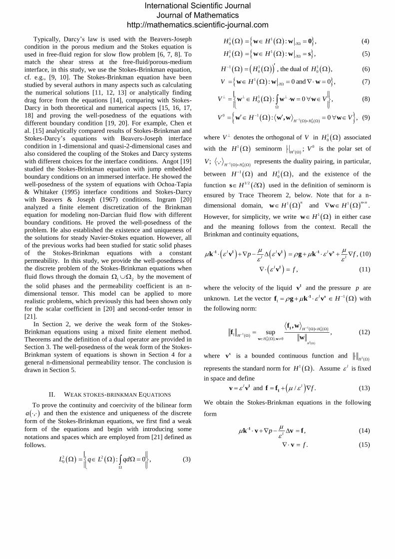
animal hair. The configuration showing the geometry of our

model is illustrated in Figure 1. It displays an ideal cell of

moving solid phases in domain 1 and free-fluid region

2

resides above 1.

Fig. 1. A snapshot of a cell of a free-fluid region resides above the porous medium.

A model using an upscaling technique is employed so that we

do not have to consider the motion of each individual moving

solid phases but rather what all solid phases do collectively

and can be viewed as a porous medium with the self-propelled

solid phase. We employ the coupled Stokes-Brinkman system

[2, 3]:

l l

lp

-1 l l

k v vl

lf

-1 s

g k v , (1)

l lv ,f (2)

where / 1 ;l l lf sv is a dynamic viscosity;

-1k is the inverse of the permeability tensor; l is the

porosity; lv and s

v are the velocities of the liquid and solid

phases, respectively; p is the pressure; 0.5T

l l ld v v

is the rate of deformation tensor; is the fluid density; g is

the gravity; l is the material time derivative of the porosity

with respect to the solid phase, / .l l lt sv The

introduction of an effective viscosity parameter, / ,l in the

additional term of Darcy’s law within the Brinkman equation

allows the matching of the stress between the two domains.

Without the inverse of the permeability term,

l l -1 l sk v v and the source term ,f the Brinkman

equation becomes the Stokes equation. With divergence-free

condition, this is the case in 2 while the Brinkman equation

with the nondivergence form (2) is used in 1. The system of

equations is derived from Hybrid Mixture Theory (HMT) [4,

5], which is an upscaling method. The derivation of the

momentum equation can be found in [2] while the derivation

of the conservation of mass, equation (2), used in this problem

is in [3, 5]. In this work, we present the existence and

uniqueness of the Stokes-Brinkman equations for the

numerical problem when the permeability coefficient is an

n-dimensional tensor.

International Scientific Journal Journal of Mathematics

http://mathematics.scientific-journal.com

Typically, Darcy’s law is used with the Beavers-Joseph

condition in the porous medium and the Stokes equation is

used in free-fluid region for slow flow problem [6, 7, 8]. To

match the shear stress at the free-fluid/porous-medium

interface, in this study, we use the Stokes-Brinkman equation,

cf. e.g., [9, 10]. The Stokes-Brinkman equation have been

studied by several authors in many aspects such as calculating

the numerical solutions [11, 12, 13] or analytically finding

drag force from the equations [14], comparing with Stokes-

Darcy in both theoretical and numerical aspects [15, 16, 17,

18] and proving the well-posedness of the equations with

different boundary condition [19, 20]. For example, Chen et

al. [15] analytically compared results of Stokes-Brinkman and

Stokes-Darcy’s equations with Beavers-Joseph interface

condition in 1-dimensional and quasi-2-dimensional cases and

also considered the coupling of the Stokes and Darcy systems

with different choices for the interface conditions. Angot [19]

studied the Stokes-Brinkman equation with jump embedded

boundary conditions on an immersed interface. He showed the

well-posedness of the system of equations with Ochoa-Tapia

& Whitaker (1995) interface conditions and Stokes-Darcy

with Beavers & Joseph (1967) conditions. Ingram [20]

analyzed a finite element discretization of the Brinkman

equation for modeling non-Darcian fluid flow with different

boundary conditions. He proved the well-posedness of the

problem. He also established the existence and uniqueness of

the solutions for steady Navier-Stokes equation. However, all

of the previous works had been studied for static solid phases

of the Stokes-Brinkman equations with a constant

permeability. In this study, we provide the well-posedness of

the discrete problem of the Stokes-Brinkman equations when

fluid flows through the domain 1 2 by the movement of

the solid phases and the permeability coefficient is an n-

dimensional tensor. This model can be applied to more

realistic problems, which previously this had been shown only

for the scalar coefficient in [20] and second-order tensor in

[21].

In Section 2, we derive the weak form of the Stokes-

Brinkman equations using a mixed finite element method.

Theorems and the definition of a dual operator are provided in

Section 3. The well-posedness of the weak form of the Stokes-

Brinkman system of equations is shown in Section 4 for a

general n-dimensional permeability tensor. The conclusion is

drawn in Section 5.

II. WEAK STOKES-BRINKMAN EQUATIONS

To prove the continuity and coercivity of the bilinear form

,a and then the existence and uniqueness of the discrete

form of the Stokes-Brinkman equations, we first find a weak

form of the equations and begin with introducing some

notations and spaces which are employed from [21] defined as

follows.

2

0L 2 : 0 ,q L qd

(3)

1

0H 1 : ,H w w 0 (4)

1

sH 1 : ,H w w s (5)

1H 1 1

0 0, the dual of ,H H

(6)

V 1 : 0 and 0 ,H w w w (7)

V 1

0 : 0 ,H V

w w w w (8)

0V 1 1

0

1 : 0 ,H H

H V

w w ,w w (9)

where V denotes the orthogonal of V in 1

0H associated

with the 1H seminorm 1

0;H

V

is the polar set of

1 10

; ,H H

V represents the duality pairing, in particular,

between 1H and 1

0 ,H and the existence of the

function 1/2H s used in the definition of seminorm is

ensured by Trace Theorem 2, below. Note that for a n-

dimensional domain, 1 nH w and 1 .

n nH

w

However, for simplicity, we write 1H w in either case

and the meaning follows from the context. Recall the

Brinkman and continuity equations,

l l

lp

-1 l l

k v v ,l

lf

-1 s

g k v (10)

l lv ,f (11)

where the velocity of the liquid lv and the pressure p are

unknown. Let the vector 1

l -1 sf g k v 1H with

the following norm:

1 10

1

10

1

1, 0

sup ,

H

H H

HH

1

w w

f ,wf

w (12)

where sv is a bounded continuous function and

1H

represents the standard norm for 1 .H Assume l is fixed

in space and define l l

v v and / .l f 1

f f (13)

We obtain the Stokes-Brinkman equations in the following

form

l

p

-1k v v , f (14)

v .f (15)



Define the linear and bilinear functionals

,a v w : ,l

-1

v w k v w (16)

,b qv ,q

v (17)

1c w 1 1

01, ,

lH Hf

f w w (18)

2c q .fq

(19)

Then, the weak formulation of (14) and (15) can be expressed

as follows.

Problem 1. (Weak Stokes-Brinkman) Find 1

sH v and

2

0p L such that

1

0 ,H w , ,pa bv w w 1 ,c w (20)

2

0 ,q L ,b pv 2 .c q (21)

III. Preliminary definition and theorems

In this section, we present selected definitions, lemmas and

theorems required to use in the proof of the well-posedness of

the weak form of our model to make this paper self-contained

though they are provided in several places such as [20] and

[21] while the definitions of Sobolev norm, seminorm and

weak derivative are based on [22]. We first introduce the

direct and inverse trace theorem for 1H as follows [23].

Theorem 2. (Direct and Inverse Trace Theorem for 1H )

There exist positive constants K and K such that, for each

1 ,H w its trace on belongs to 1/2H and

1/2 1 .H H

K

w w Conversely, for each given function

1/2 ,H s there exists a function 1H s

v such that

its trace on coincides with s and

1 1/2 .H H

K

s

v s (22)

This theorem ensures that if 1/2 ,H s then there

exists 1H s

v such that the trace of s

v on is .s The

following formulation will be used in the proof of the

Theorem 8.

Theorem 3. 1

0 0! V H v such that 0 .f

sv v

Proof. The proof of this theorem is provided in [21].

Next theorem states that the divergence operator is an

isomorphism between 2

0L and ,V and the

Ladyzhenskaya-Babuška-Brezzi (LBB) condition, which is

required for the stability of a mixed finite element method, is

mentioned [24, 25].

Theorem 4. Let be connected. Then

1) the operator grad is an isomorphism of 2

0L onto 0 ,V

2) the operator div is an isomorphism of V onto 2

0 .L

Moreover, there exists 0 such that

2

10 1 20

,inf sup 0

q L HH L

b q

q

w

w

w (23)

and for any 2

0 ,q L there exists a unique

1

0V H v satisfying

1 2

1 .H L

q

v (24)

Note that the equation (23) is known as the LBB condition

[25]. We next state the definition of linear operators and their

dual operator and then rewrite the Problem 1 in the form of the

linear operator. This simple change allows us to prove the

existence and uniqueness of the pressure term. Recall that the

dual spaces of 2

0L and 1H are 2

0L

and 1

0 ,H

respectively, i.e., 2 2

0 0L L

and 1 1

0 .H H

Definition 5. Let 1, H v w and 2

0 .q L Define

linear operators 1 1

0:A H H and 1 2

0 0:B H L

by

1 10

, :H H

A v w ,a v w , 1

0, H v w (25)

1 20 0

, :H L

B q

v ,b q v , 1 2

0 0, .H q L v (26)

Let 2 1

0 ;B L H L be the dual operator of ,B i.e.

, , :B q q B v v , ,b q v 1 2

0 0, .H q L v (27)

With these operators, Problem 1 is equivalently written in the

form:

Problem 6. Find 1 2

0,sH p L v such that

A B p v f in 1H (28)

B fv in 2

0 .L (29)



IV. WELL-POSEDNESS OF THE STOKES-BRINKMAN

PROBLEM

Even though Ingram [20] and [21] proved the well-

posedness of the Stokes-Brinkman problem, it was for only

with a constant and second-tensor permeability, respectively.

Here we generalize the result of the discrete equations when

k is an n-dimensional tensor. To present the well-posedness

of the Stokes-Brinkman equations, we first show that the

linear and bilinear functionals (16)-(19) are continuous and

,a is coercive. Then we use these properties to show the

existence and uniqueness of the equations in Theorem 8

below.

Theorem 7. The linear functionals 1 2, c c qw and

bilinear functionals , , ,a b are continuous and ,a

is coercive, i.e.,

1

2, c H

a C

w w w (30)

where min / , ;c k kC C C is a positive number. In

particular,

1 2 11 ,

H L Hc n f

1w f w

1 ,H w (31)

2 22 ,

L Lc q f q

2 ,q L (32)

1 2, ,

H Lb q n q

v v 1 ,H v

2 ,q L (33)

1 1, ,a H H

a C

v w v w 1 ,H v

1 ,H w (34)

where n is the dimensional number and

1

1 ,max / , max .l

a i j n ijC n k

Proof. Since the linearity of 1c w and 2c q and bilinearity

of ,a v w and ,b qv are obvious and the continuities of

1 2,c c qw and ,b qv have been shown in [21], we next

show ,a v w is continuous. To prove the continuity of

,a v w for an n-dimensional domain, we first introduce

Young’s inequality: / /p qab a p b q where , 0,a b

, 0p q and 1/ 1/ 1p q which is often used

below, write vectors v and w in component forms:

1 2, ,..., nv v vv and 1 2, ,..., nw w ww and consider

2

2

L -1

k v

2

1

1 1

n n

ij j

i j

k v

1

21 1 1

1 1 1

2n n n n

ij j ij ik j k

i j j k j

k v k k v v d

1

21 2

1 ,1 1

max 2n n n

ij k j ki j n

k j k j

n k v v v d

21

1 ,

12 22

1 1

max iji j n

n n n

k j k

k j k j

n k

v v v d

22 1 2

1 ,1

maxn

ij ki j n

k

n k v d

2

2 22 1

1 ,max ,ij Li j n

n k

v (35)

where Young’s inequality is applied to the third inequality.

We then employ the inequality (35) to complete the proof of

the continuity of ,a v w as follows.

,a v w :l

-1

v w k v w

:l

-1

v w k v w

2 2 22l L L LL

-1

v w k v w

2 2

2 2

1

1 ,max

l L L

ij L Li j nn k

v w

v w

1 1 ,a H HC

v w

where 1

1 ,max / , maxl

a iji j n

C n k

and (35) is employed to

the third inequality.

Before proving the coercivity of the bilinear form , ,a w w

we first consider, for n-dimensions,

-1k w w

11 2 1

1 1

2 .n n n

ii i ij i j

i i j i

k w k w w

(36)

Since in our problem -1k is positive definite, the diagonal

entries of -1k are positive numbers, which imply that the first

term of the right-hand side of (36) is a positive number. We

now focus on the second term 1

1

1

2 .n n

ij i j

i j i

k w w

Note that if

1 0ij i jk w w for all i and ,j it’s easy to see that

-1k w w 1 2 1 2 2

11 1 1

minn n n

ii i ii i k ii n

i i i

k w k w C w

where



1

1min .k ii

i nC k

If there exist r and s such that 1 0,rs r sk w w

we have two possible cases.

Case 1. 1 0rsk and 0.r sw w

Thus, 1 1 1 2 22 2 ,rs r s rs r s rs r sk w w k w w k w w

where Young’s inequality is applied at the inequality.

Without lose of generality, let .r s Thus,

-1k w w

11 2 1

1 1

2n n n

ii i ij i j

i i j i

k w k w w

11 2 1

1 1

1 2 1

1

2

2

n n n

ii i ij i j

i i j ii r i r

n

rr r ri r i

i r

k w k w w

k w k w w

11 2 1

1 1

1 2 1

11

1 2 2 1

2

2 ...

... 2

n n n

ii i ij i j

i i j ii r i r

rr r r rr r

rs r s rn r n

k w k w w

k w k w w

k w w k w w

11 2 1

1 1,

1 1 2 1 1 2

1 1

1 11 1

1 1

11

2

2 ... 2

2 ... 2

n n n

ii i ij i j

i i j ii r s i r

rr rs r ss rs s

r r r sr r r s

r s rn r nr s

k w k w w

k k w k k w

k w w k w w

k w w k w w

2

1

,n

k i

i

C w

where

1 1 1 1min , , min ,k k k k rr rs ss rsC d b b k k k k

and 1

1,

min .k iii n

i r s

d k

Note that 0kb because -1k is a

diagonally dominant matrix. Therefore,

2

1

.n

k i

i

C w

-1k w w

Case2. 1 0rsk and 0.r sw w

Since -1k is bounded, 0bC such that 1 .rs bk C

Thus, 1 2 22 2 .rs r s b r s b r sk w w C w w C w w

Thus, -1k w w

11 2 1

1 1

2n n n

ii i ij i j

i i j i

k w k w w

11 2 1

1 1

1 2 1

1

2

2

n n n

ii i ij i j

i i j ii r i r

n

rr r ri r i

i r

k w k w w

k w k w w

11 2 1 1 2

1 1

1 2 2 1

11

2

2 ... ... 2

n n n

ii i ij i j rr r

i i j ii r i r

r r b r s rn r nr r

k w k w w k w

k w w C w w k w w

11 2 1 1 2

1 1,

1 2 1 1

1 11 1

1 1

11

2

2 ... 2

2 ... 2

n n n

ii i ij i j rr b r

i i j ii r s i r

ss b s r r r sr r r s

r s rn r nr s

k w k w w k C w

k C w k w w k w w

k w w k w w

2

1

,n

k i

i

C w

where

1 1min , , min , 0k r r r rr b ss bC d b b k C k C

and 1

1,

min .k iii n

i r s

d k

Therefore, 2

1

.n

k i

i

C w

-1k w w

From all of the cases above, we have

2

1

0, .n

k k i

i

C C w

-1k w w (37)

Integrating (36) both sides, we obtain

2

22

1

.n

k i k Li

C w C

-1

k w w w (38)

Hence, the coercivity of the bilinear form

,a w w :l

-1

w w k w w

2 2

2 2

kl L LC

w w

1

2,c H

C

w

where min / , .c kC C We now ready to prove the existence and uniqueness of the

Stokes-Brinkman equations. Though the following theorem

have been shown in [20] and [21], we state here in the full

form of completeness.

Theorem 8. (Well-posedness of the Stokes-Brinkman

equations) Assume that 1

1 ,H f 2, f L f and

1/2 .H s There exists a unique 1 2

0,sH p L v

satisfying Problem 1, equations (20)-(21). Moreover,

1 1 2 11

1ˆ1a

H H L H

c c

Cn f

C C

v f v (39)

where 0ˆ sv v v and

2 1 2 11

1 1.alL H L H

p n f C

f v (40)

where is the constant in (23).



Proof. We note that the proof of the inequalities (39) and (40)

are provided in [21]. Here we show the existence and

uniqueness of the velocity by using Lax-Milgram theorem

while the well-posedness of the pressure are shown in the

second part by employing Theorem 4 and the definition of

linear operators and their dual operators.

Restrict 1 2

1 , ,H f L f f and 1/2 .H s

From Theorem 3, we let 0

ˆ . s

v v v For any ,Vw let

1ˆ , .F c a w w v w Since 1c is linear and ,a is

bilinear, F is linear. Moreover, the continuities of 1c

and ,a imply that F is continuous. By employing Lax-

Milgram theorem, there exists a unique 1

0V H v such

that , .a Fv w w Define . s 0

v v v v Because

1

0 ,V H 0

v and 1

0 , .V H v v s Since

Vv and , .f f 0 s

v v v We now have

1

sH v satisfying the continuity equation.

Next we show that v is unique. Since

1ˆ, ,a F c a v w w w v w and ˆ , v v v ,a v w

1 .c w Let 1

v and 2

v satisfy 1,a c1

v w w and

1, .a c2

v w w Then , 0a 1 2

v v w for any .Vw

Thus, , 0.a 1 2 1 2

v v v v Therefore 0 ,a 1 2 1 2

v v v v

1

20.c H

C

1 2

v v Since 10, 0.c H

C

1 2

v v

Then 1 2v = v in the 1H -norm.

To show that there exists 2

0p L satisfying Problem 1

or 6, we define 1F such that 1 1, .F cw w Since

1ˆ, , ,a c a v w w v w 1

ˆ, , 0c a a w v w v w or

1ˆF A A v v 0, in operator notation, 0

1ˆ .F A A V v v

Let 2 0

0: .B L V From Theorem 4 and the

isomorphic property, there exists a unique 2

0p L such

that 1 1

ˆB p F A A F A v v v or 1.A B p F v

V. CONCLUSION

In this study, we employ the macroscale Stokes-Brinkman

equation for coupled free-fluid/porous-medium viscous flow

using Hybrid Mixture Theory and nondimensionalization.

The system of equations is established for the porous medium

containing moving solid phases such as hairlike structure. We

show that the bilinear form ,a is continuous and coercive

for n-dimensional permeability coefficient while it is

presented in [20] only for a constant coefficient and in [21] for

a second-order tensor. We also present the existence and

uniqueness of the Stokes-Brinkman system of equations

although this is provided in [21]. Numerical solutions of this

model using a mixed finite element method will be provided

in future work.

ACKNOWLEDGMENT

This research was supported by a grant from KMITL

Research Fund (KMITL Fund)

REFERENCES

[1] S. A. Mattis, C. N. Dawson, C.E. Kees, W. Farthing, “Numerical

Modeling of Drag for Flow through Vegetated Domains and Porous Structures”, Advances in Water Resources 39, 2012, pp. 44-59.

[2] K. Chamsri, “N-Dimensional Stokes-Brinkman Equations using a Mixed Finite Element Method”, Australian Journal of Basic and Applied Science 8(11), Soecial 2014, pp.30-36.

[3] T. F. Weinstein, Three-Phase Hybrid Mixture Theory for Swelling Drug Delivery Systems, Ph.D. thesis, University of Colorado Denver, 2005.

[4] L. S. Bennethum, J. H. Cushman, “Multiphase, Hybrid Mixture Theory for Swelling Systems-I: Balance Laws”, International Journal of Engineering Science 34(2), 1996, pp. 125-145.

[5] T. F. Weinstein, L. S. Bennethum, “On the Derivation of the Transport Equation for Swelling Porous Materials with Finite Deformation”, International Journal of Engineering Science, 2006.

[6] T. Arbogast, D. S. Brunson, “A Computational Method for Approximating a Darcy-Stokes System Governing a Vuggy Porous Medium”, Computaional Geosciences 11, 2007, pp. 207-218.

[7] N. S. Hanspal, A. N. Waghode, V. Nassehi, R. J. Wakeman, “Numerical Analysis of Coupled Stokes/Darcy Flows in Industrial Filtrations”, Transport in Porous Media 64, 2006, pp. 73-101.

[8] W. J. Layton, F. Schieweek, I. Yotov, “Coupling Fluid Fluid Flow with Porous Media Flow”, SIAM Journal on Numerical Analysis 40, 2003, pp. 2195-2218.

[9] N. S. Martys, J. G. Hagedorn, “Multiscale Modeling of Fluid Transport in Heterogeneous Materials using Discrete Boltzmann Methods”, Materials and Structures 35, 2002, p. 650-659.

[10] G. Neale, W. Nader, “Practical Significance of Brinkman’s Extension of Darcy’s Law: Coupled Parallel Flows within a Channel and a Bounding Porous Medium”, Canadian Journal of Chemical Engineering 52, 1974, p.475-478.

[11] W. R. Hwang, S. G. Advani, “Numerical simulations of Stokes-Brinkman equations for permeability prediction of dual scale fibrous porous media”, Physics of Fluids 22, 2010.

[12] O. Iliev, Z. Lakdawala, V. Starikovicius, “On a numerical subgrid upscaling algorithm for Stokes-Brinkman equations”, Computers and Mathematics with Applications 65, 2013, pp. 435-448.

[13] N. S. Martys, “Improved Approximation of the Brinkman Equation using a Lattice Boltzmann Method”, Physics of Fluids 13, 2001, pp. 1807-1810.

[14] V. A. Kirsh, “Stokes Flow in Periodic Systems of Parallel Cylinders with Porous Permeabla Shells”, Colloid Journal 68, 2006, pp. 173-181.

[15] N. Chen, M. Gunzburger, X. Wang, “Asymptotic Analysis of the Differences between the Stokes-Darcy System with Different Interface Conditions and the Stoke-Brinkman System”, Journal of Mathematical Analysis and Applications 368, 2010, pp. 658-676.

[16] X. Xu, S. Zhang, “A New Divergence-Free Interpolation Operator with Applications to the Darcy-Stoke-Brinkman Equation”, Society for Industrial and Applied Mathematics 32, 2010, pp. 855-874.

[17] M. Chandesris, D. Jamet, “Boundary Conditions at a Fluid-Porous Interface: An a Priori Estimation of the Stress Jump Coefficients”, International Journal of Heat and Mass Transfer 50, 2007, pp. 3422-3436.

[18] H. Tan, K. M. Pillai, “Finite Element Implementation of Stress-Jump and Stress-Continuity Conditions at Porous-Medium”, Clear-Fluid Interface, Computers&Fluids 38, 2009, pp. 1118-1131.

[19] P. Angot, “On the well-posed coupling between free fluid and porous viscous flows”, Preprint submitted to Applied Mathematics Letters (REVISED VERSION), 2009.



[20] R. Ingram, “Finite Element Approximation of Nonsolenoidal, Viscous Flows around Porous and Solid Obstacles”, The SIAM Journal on Numerical Analysis 49, 2011, pp. 491-520.

[21] K. Chamsri, Modeling the Flow of PCL Fluid due to the Movement of Lung Cilia, Ph.D. thesis, University of Colorado Denver, 2012.

[22] S. C. Brenner, L. R. Scott, The Mathematical Theory of Finite Element Methods, Springer-Verlag, 1994.

[23] E. G. Dyakonov, S. McCormick, Optimization in Solving Elliptic Problems, CRC Press, 1995.

[24] V. Girault, P. Raviart, Finite Element Methods for Navier-Stokes Equations Theory and Algorithms, Springer-Verlag, 1986.

[25] F. Brezzi, M. Fortin, Mixed and Hybrid Finite Element Methods, Springer-Verlag, 1991.



Formulation of a Well-Posed Stokes-Brinkman Problem with a...

Documents

Transcript of Formulation of a Well-Posed Stokes-Brinkman Problem with a...