Formulation, General Features and Global Calibration of a ...

RESEARCH ARTICLE

Formulation, General Features and GlobalCalibration of a Bioenergetically-ConstrainedFishery ModelDavid A. Carozza¤a*, Daniele Bianchi¤b, Eric D. Galbraith¤c¤d

Department of Earth and Planetary Sciences, McGill University, Montreal, Quebec, Canada

¤a Current address: Department of Mathematics, Universite du Quebec àMontreal, Montreal, Canada¤b Current address: Department of Atmospheric and Oceanic Sciences, University of California, LosAngeles, Los Angeles, United States of America¤c Current address: Institucio Catalana de Recerca i Estudis Avancats (ICREA), 08010 Barcelona, Spain¤d Current address: Institut de Ciència i Tecnologia Ambientals (ICTA) and Department of Mathematics,Universitat Autonoma de Barcelona, 08193 Barcelona, Spain* [email protected]

Abstract

Human exploitation of marine resources is profoundly altering marine ecosystems, while cli-

mate change is expected to further impact commercially-harvested fish and other species.

Although the global fishery is a highly complex system with many unpredictable aspects, the

bioenergetic limits on fish production and the response of fishing effort to profit are both rela-

tively tractable, and are sure to play important roles. Here we describe a generalized, cou-

pled biological-economic model of the global marine fishery that represents both of these

aspects in a unified framework, the BiOeconomic mArine Trophic Size-spectrum (BOATS)

model. BOATS predicts fish production according to size spectra as a function of net primary

production and temperature, and dynamically determines harvest spectra from the biomass

density and interactive, prognostic fishing effort. Within this framework, the equilibrium fish

biomass is determined by the economic forcings of catchability, ex-vessel price and cost per

unit effort, while the peak harvest depends on the ecosystem parameters. Comparison of a

large ensemble of idealized simulations with observational databases, focusing on historical

biomass and peak harvests, allows us to narrow the range of several uncertain ecosystem

parameters, rule out most parameter combinations, and select an optimal ensemble of

model variants. Compared to the prior distributions, model variants with lower values of the

mortality rate, trophic efficiency, and allometric constant agree better with observations. For

most acceptable parameter combinations, natural mortality rates are more strongly affected

by temperature than growth rates, suggesting different sensitivities of these processes to cli-

mate change. These results highlight the utility of adopting large-scale, aggregated data

constraints to reduce model parameter uncertainties and to better predict the response of

fisheries to human behaviour and climate change.

PLOS ONE | DOI:10.1371/journal.pone.0169763 January 19, 2017 1 / 28

a1111111111a1111111111a1111111111a1111111111a1111111111

OPENACCESS

Citation: Carozza DA, Bianchi D, Galbraith ED(2017) Formulation, General Features and GlobalCalibration of a Bioenergetically-ConstrainedFishery Model. PLoS ONE 12(1): e0169763.doi:10.1371/journal.pone.0169763

Editor: Vanesa Magar, Centro de InvestigacionCientifica y de Educacion Superior de EnsenadaDivision de Fisica Aplicada, MEXICO

Received: June 1, 2016

Accepted: December 21, 2016

Published: January 19, 2017

Copyright: © 2017 Carozza et al. This is an openaccess article distributed under the terms of theCreative Commons Attribution License, whichpermits unrestricted use, distribution, andreproduction in any medium, provided the originalauthor and source are credited.

Data Availability Statement: All data files areavailable from the Zenodo database at http://dx.doi.org/10.5281/zenodo.53934. We provide theMATLAB functions, fisheries data, model forcingdata (net primary production and temperature),and model output required to generate the figuresand do calculations. The plot and analysis script iswritten in MATLAB version R2012a.

Funding: This research was supported by theSocial Sciences and Humanities Research Councilof Canada through a Joseph-Armand Bombardier

http://crossmark.crossref.org/dialog/?doi=10.1371/journal.pone.0169763&domain=pdf&date_stamp=2017-01-19






http://creativecommons.org/licenses/by/4.0/

http://dx.doi.org/10.5281/zenodo.53934

http://dx.doi.org/10.5281/zenodo.53934

Introduction

Global oceanic wild fish harvest grew at a tremendous rate over the 20th century, increasingby approximately a factor of four between 1950 and 1990 [1]. As a result, biomass has beendepleted relative to its pristine state [2, 3], altering ecosystem structures worldwide, with col-lapses documented in between 7 and 25% of fisheries [4, 5]. Anthropogenic climate change isaltering primary production and temperature distributions worldwide [6], with impacts on theranges of various marine species [7, 8], and on their growth, mortality, reproduction, andrecruitment rates [9, 10]. Meanwhile, rapid and ongoing changes in fishing technology [11],the demand for fish products [12], and regulation frameworks are driving changes in the dis-tribution and intensity of fishing effort. Given future projections of increasing human popula-tion, and consequent pressure on food resources, it is critical to develop improved predictiveunderstanding of how fisheries will evolve with interacting environmental and human drivers.

Numerical models of fishery-human interactions that can be coupled to representations ofthe environment, often called end-to-end models, have been extremely helpful to shed light onthese issues [13, 14]. However, most of these models are designed primarily in order to studyinternal ecosystem dynamics, and often include complex parameterizations that are challengingto quantify, such as feeding relationships [15]. In addition, most of these models are designed torepresent the present-day community in a specific region, and therefore lack the generality andflexibility required to represent long-term structural changes such as those caused by new inva-sive species, climate-driven range shifts [7], or fishing-driven evolution [16]. The incompleteview provided by a patchwork of regional models also hampers studies of global food security,given the development of globally interwoven fishing fleets and fish-trading since the 1950’s.

Alternative ecological models that are structurally simpler, founded on macroecologicalprinciples, and appropriate for a global range of conditions, have recently begun to allow thedirect prediction of fish biomass from environmental variables [17–23]. However, most ofthese models were designed to study fish, rather than fishing. As a result, fish harvests are gen-erally prescribed in these models, rather than treating the fishing effort as an interactive com-ponent, which limits the consideration of economic factors such as changes in fishingtechnology, market conditions, and regulatory regimes. Furthermore, an extensive explorationof parameter uncertainty is challenging for most of these models due to complexity and/orcomputational cost, and the simulated fish species may not be equivalent to those harvested,making direct comparisons with observed historical harvest records difficult.

Here we describe the economic component and general characteristics of the BiOeconomicmArine Trophic Size-spectrum model (BOATS), a computationally-efficient model whichdirectly couples a size spectrum model of fish biomass with an interactive economic model on aspatially-resolved global grid. The ecological model, which is described in detail in [24], focuseson a small number of robust bioenergetic principles of marine ecosystems that are of direct rele-vance for fisheries and environmental change, predicting the growth of all commercially-har-vested marine consumers, which we refer to as ‘fish’. The simulated fish spectrum is coupleddirectly to a prognostic model of fishing effort, at the same grid scale, that evolves over time inresponse to the local bioeconomically-determined profit. Because BOATS was designed toinclude only fundamental processes and relatively few parameters, parameter uncertainty canbe addressed in a robust and comprehensive way by using a Monte Carlo approach. As dis-cussed below, this allows us to select global parameter combinations that agree with observa-tions at the scale of the Large Marine Ecosystems (LMEs), rather than being locally-tuned. Weshow that, after optimization, the ensemble has a high degree of skill, making it suitable forstudies of first-order interactions between climate, the marine ecosystem and humans. We alsopoint out the most important implications of the remaining parameter uncertainty.

Formulation, General Features and Global Calibration of a Bioenergetically-Constrained Fishery Model


Canada Graduate Scholarship (SSHRC, www.sshrc-crsh.gc.ca/home-accueil-eng.aspx), by theMarine Environmental Observation Prediction andResponse Network (MEOPAR, http://meopar.ca)for a doctoral fellowship and operational support,the Birks Family Foundation for a doctoral bursary(http://birksfamilyfoundation.ca), the friends ofCaptain O.E. LeRoy and the Department of Earthand Planetary Sciences for a LeRoy MemorialFellowship in Earth and Planetary Sciences (www.mcgill.ca/eps/home). This research was alsosupported by the Canada Foundation for Innovation(CFI, www.innovation.ca) and Compute Canada(www.computecanada.ca) for computinginfrastructure. This project has received fundingfrom the European Research Council (ERC) underthe European Union’s Horizon 2020 research andinnovation programme (grant agreement No682602). The funders had no role in study design,data collection and analysis, decision to publish, orpreparation of the manuscript.

Competing Interests: The authors have declaredthat no competing interests exist.

http://www.sshrc-crsh.gc.ca/home-accueil-eng.aspx

http://www.sshrc-crsh.gc.ca/home-accueil-eng.aspx

http://meopar.ca

http://birksfamilyfoundation.ca

http://www.mcgill.ca/eps/home

http://www.mcgill.ca/eps/home

http://www.innovation.ca

http://www.computecanada.ca

Materials and Methods

Model description

Overview. The guiding principles during the development of the BiOeconomic mArineTrophic Size-spectrum (BOATS) model were: 1. To maintain general applicability to a broadrange of marine ecosystems and fisheries; 2. To include sufficient ecological complexity to rep-resent the fundamental dynamics of commercial fish biomass production, but remain simpleenough to be easily interpretable; 3. To minimize the number of uncertain parameters; 4. Toinclude a dynamical representation of fishing activity in the same framework as the ecosystem;5. To enable long-term projections of the coupled natural-social system with robust and simpleexternal forcings.

Fig 1 gives a schematic representation of the model. Biomass production is determined bythe energy supplied from photosynthesis [25], the life history of individuals according to tem-perature-dependent growth and mortality rates [26, 27], and stock-productivity-dependentrecruitment [28]. Feeding relationships are not explicit, a simplifying assumption motivatedby the diversity of marine life and predatory strategies, and the heterogeneity of species inter-relationships in different regions. Life history is resolved in terms of growth from juveniles toreproductively-mature individuals, through a continuous spectrum of size.

Fig 1. Schematic diagram of the main modules, components, and processes of the BOATS model.

doi:10.1371/journal.pone.0169763.g001



The model is deterministic, discretized on a 2-dimensional spatial grid (representing thevertically-integrated ecosystem), and steps forward in time from a set of initial conditions. Themodel can include an arbitrary number of size spectra, each of which represents a ‘super-organism’ that exists in all grid cells at all times. There is no simulation of horizontal move-ment by fish or fishing boats, so that each cell is independent (that is, no interaction with othercells). Although this ignores the life history aspects of larval transport and migration, such asimportant environmental contrasts between spawning grounds and adult feeding grounds[29], these were determined to be difficult problems when considering all types of commercialspecies, and resolving movement would incur a large computational burden [21]. Fishingeffort is interactively determined in each grid cell, and evolves over time as a function of theharvest in that grid cell, dependent on globally-constant economic forcings. In the following,we refer to globally-constant scalars that determine the behavior of a model but do not varyduring or between simulations as ‘parameters’, and to a model with a particular set of parame-ters as a ‘model variant’. Prescribed quantities that influence the model behaviour and mayvary during or between simulations are referred to as ‘forcings’ (which may be globally homog-enous, or locally variable), while model state variables are referred to as ‘variables’. Keyassumptions are summarized in Table 1.

Below, we elaborate on details of the model. First, we present a brief overview of the ecosys-tem module formulation and equations, and refer the reader to [24] for a full description. Sec-ond, we describe the dynamic determination of fishing effort. Third, we discuss the allocationof effort over the size spectra, representing the selectivity of fishing gear.

Ecological module. BOATS resolves an arbitrary number of size spectra that are definedby their asymptotic sizes and, together, are defined as the sum of all consumers (includingboth finfish and invertebrates) that were commercially harvested before the year 2006. Herewe discretize the commercial species among three spectra, which we refer to as small, medium,and large groups, referring to their asymptotic size.

Table 1. Key model assumptions.

Essential Present version (could be changed)

Ecosystem

Mass is the ecological organizing variable Community represented by 3 spectra with different asymptotic sizes

Biomass individual flux follows the McKendrick-von Foersterequation

No movement of fish between grid cells

Asymptotic size is the spectrum-defining trait Implicit feeding relationships

Production dependent on NPP, T, and stock-dependentrecruitment

Fish spawn continuously

Individual fish growth cannot exceed a physiological upper limit Potentially-commercial species aggregated by size (finfish andinvertebrates)

Economics

Fishing effort is the fundamental economic variable Open access (no management)

Technology determines catchability Local effort varies with the profitability of fishing at that point

Effort and biomass determine harvest through catchability Harvest is linear in effort and biomass

Selectivity function determines the size-structure of harvest No movement of fishing vessels between grid cells

Fleet dynamics parameter is globally constant

Cost per unit effort is globally constant

Price is globally constant, and does not vary by group or size

Catchability is globally constant, but is varied over time

doi:10.1371/journal.pone.0169763.t001



The evolution of biomass in each group spectrum is represented using the McKendrick-von Foerster model [30, 31],

@

@tfk à � @

@mgkfk á

gkfk

m� Lkfk; Ö1Ü

where m is the individual fish mass, t is time, fk (gwB m−2 g−1, where gwB are grams of wet bio-mass) is the biomass spectrum of group k, γk (g s−1) the group growth rate, and Λk (s−1) thegroup natural mortality rate.

Fish biomass growth rates are limited by a production spectrum that estimates the energy(here assumed to be equivalent to biomass) that can be provided to any given size through tro-phic transfer from primary production ξP,k (g s−1) [18, 25, 32], and are also limited by allome-tric estimates of the rates at which individual fish can grow ξVB,k (g s−1) [28, 33, 34].Underlying the simulated biomass spectra are the calculated flows of biomass energy fromphotosynthesis to fish via the trophic transfer, which we express as

xP;k à�C;kpm

fk; Ö2Ü

where π (gwB m−2 g−1 s−1) is the spectrum of energy from primary production available toeach individual of size m that depends on the trophic scaling τ as the exponent of a power lawdependence, and ϕC,k is the fraction of primary production allocated to a commercial group k[18, 25, 32]. Furthermore, we assume that the flow of biomass energy from small to large fish,which occurs as individuals grow according to empirical allometric rules, cannot exceed amaximum physiological rate

xVB;k à Amb � kam; Ö3Ü

where b (unitless) is the allometric scaling constant, A (g s−1) is the allometric growth rate, andka (s−1) is the mass specific investment in activity [28, 33, 34]. The allometric growth rate A isthe product of a temperature-independent rate A0 (g1−b s−1) and a van’t Hoff–Arrhenius(exponential) temperature dependence aA(T) which is set by the growth activation energy ofmetabolism ωa,A (eV) parameter [25].

The realized input energy to growth and reproduction in each size class, ξI (g s−1), is theminimum of ξP and ξVB. This implies that, given an excess of food, individual fish will grow asfast as biologically possible, given their temperature-dependent metabolism. If, instead, theproduction of food at a given location is insufficient to fully feed the existing biomass, this pro-duction will be equally partitioned among all individuals and will limit growth rates. Whenthere is no harvest applied, primary production, and thus ξP, generally limits growth over thebiomass spectrum.

The natural mortality rate Λk is based on an empirical relationship that depends on theindividual and asymptotic mass, and is first order in fish biomass, according to

Lk à lm�hmháb�11;k ; Ö4Ü

where h is the mortality allometric scaling and m1,k is the asymptotic mass of group k [26, 27].The component of the mortality rate that is independent of mass, λ, is proportional to

ez1 A0alÖTÜ, where z1 is the mortality rate parameter and aλ(T) the temperature dependence ofmortality, which, as with growth, takes the van’t Hoff–Arrhenius functional form and is set bythe mortality activation energy of metabolism parameter ωa,λ (eV).



Recruitment forms the bottom boundary condition to Eq (1), and is written as

fkÖm0ÜgkÖm0Ü à RP;kRe;k

RP;k á Re;k: Ö5Ü

where Re,k is the potential generation of new recruits from egg production, itself a function of1. the primary production and the fish biomass that is able to reproduce and 2. the fraction oflarvae that survive to the recruit size m0 [34], whereas RP,k is the potential flux of primary pro-duction input to juvenile fish.

The model is forced with two-dimensional, global, monthly climatological fields of net pri-mary production and temperature (S1 and S2 Figs). A schematic of BOATS, illustrating themain modules, components, and processes, is presented in Fig 1, and the full set of biologicalmodel parameters are presented in S1 Table.

The determination of fishing effort. Harvest depends upon fish biomass and the fishingeffort. Here, we interpret effort as the combined inputs used in the fishing process [35], essen-tially fuel, labour and the construction and maintenance of fishing fleets, and we express it inenergy units of W m−2 (1 W = 1 J s−1). This choice facilitates comparison with the global effortdatabase of [1, 36]. Effort of this type is often described as ‘nominal effort’, and is defined hereas being independent of fishing technology.

The allocation of fishing effort, that is, the dynamics of fleets of fishing vessels, involves bio-logical, social, and economic aspects that depend on numerous variables that operate on a vari-ety of timescales [37, 38]. In order to provide a first step in prognostic modeling of theseinteractions in a simple yet robust way, we couple the Gordon-Schaeffer open-access fisherieseconomics model [39, 40] to our ecological model [24] in a discrete, temporally-resolvedframework. This open-access model assumes an absence of regulation, so that fishermen tendto individually seek the greatest total harvest [39, 41], which ultimately leads to overharvestand to the tragedy of the commons [42, 43]. Although this is not an economically or biologi-cally optimal outcome, it is common, given the difficulty in establishing property rights overliving marine resources. Although management has made great advances in effectively coun-teracting this tendency in some fisheries, particularly since the 1990s [44, 45], the open-accessresult has historically dominated, and remains a cause of overfishing in many open-ocean andcoastal fisheries [46]. Subsidies can also shift behaviour from the open-access solution,although wherever subsidies are capacity-building they often exacerbate the open-access prob-lem [47].

In open-access fisheries, fishermen seek to maximize their individual harvests, and so aredriven by average instead of marginal profit [39]. Effort in a fish group k, Ek(t) (W m−2), there-fore evolves in time as a linear function of the average profit (profit per unit effort), as

ddt

EkÖtÜ à keâaverage profitäk àkeârevenuek � costkä

EkÖtÜ; Ö6Ü

where κe (W2 m−2 $−1) is the fleet dynamics parameter [48] that determines the timescale atwhich a change in average profit affects effort, and revenue and cost are in units of $ m−2 s−1.The fleet dynamics parameter κe is set so that the adjustment of effort to changes in profit isapproximately 10 years, since fleets adjust to changes in biomass on roughly decadal timescales[49–51]. Although the entry of effort into fisheries often occurs at a faster rate than exit, partic-ularly when subsidies are applied, for simplicity we assume here that both rates are the same.

We assume that harvest is linear in both biomass and effort, and so for a given level of har-vesting technology, a fixed amount of effort always catches the same fraction of biomass [40].The ecological model discretizes biomass along a size spectrum, and so we define an analagous



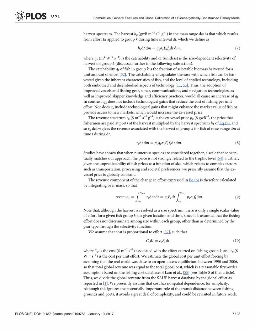
harvest spectrum. The harvest hk (gwB m−2 s−1 g−1) in the mass range dm is that which resultsfrom effort Ek applied to group k during time interval dt, which we define as

hkdt dm à qkskEkfkdt dm; Ö7Ü

where qk (m2 W−1 s−1) is the catchability and σk (unitless) is the size-dependent selectivity ofharvest on group k (discussed further in the following subsection).

The catchability qk of fish in group k is the fraction of selectable biomass harvested for aunit amount of effort [52]. The catchability encapsulates the ease with which fish can be har-vested given the inherent characteristics of fish, and the level of applied technology, includingboth embodied and disembodied aspects of technology [11, 53]. Thus, the adoption ofimproved vessels and fishing gear, sonar, communications, and navigation technologies, aswell as improved skipper knowledge and efficiency practices, would all cause an increase of qk.In contrast, qk does not include technological gains that reduce the cost of fishing per uniteffort. Nor does qk include technological gains that might enhance the market value of fish orprovide access to new markets, which would increase the ex-vessel price.

The revenue spectrum rk ($ m−2 s−1 g−1) is the ex-vessel price pk ($ gwB−1, the price thatfishermen are paid at port) of the harvest multiplied by the harvest spectrum hk of Eq (7), andso rk dtdm gives the revenue associated with the harvest of group k for fish of mass range dm attime t during dt,

rkdt dm à pkqkskEkfkdt dm: Ö8Ü

Studies have shown that when numerous species are considered together, a scale that concep-tually matches our approach, the price is not strongly related to the trophic level [54]. Further,given the unpredictability of fish prices as a function of size, which relates to complex factorssuch as transportation, processing and societal preferences, we presently assume that the ex-vessel price is globally constant.

The revenue component of the change in effort expressed in Eq (6) is therefore calculatedby integrating over mass, so that

revenuek àZ m1;k

m0

rkdm dt à qkEkdtZ m1;k

m0

pkskfkdm: Ö9Ü

Note that, although the harvest is resolved as a size spectrum, there is only a single scalar valueof effort for a given fish group k at a given location and time, since it is assumed that the fishingeffort does not discriminate among size within each group, other than as determined by thegear type through the selectivity function.

We assume that cost is proportional to effort [37], such that

Ckdt à ckEkdt; Ö10Ü

where Ck is the cost ($ m−2 s−1) associated with the effort exerted on fishing group k, and ck ($W−1 s−1) is the cost per unit effort. We estimate the global cost per unit effort forcing byassuming that the real world was close to an open-access equilibrium between 1990 and 2006,so that total global revenue was equal to the total global cost, which is a reasonable first-orderassumption based on the fishing cost database of Lam et al., [55] (see Table 5 of that article).Thus, we divide the global revenue from the SAUP harvest database by the global effort asreported in [1]. We presently assume that cost has no spatial dependence, for simplicity.Although this ignores the potentially-important role of the transit distance between fishinggrounds and ports, it avoids a great deal of complexity, and could be revisited in future work.



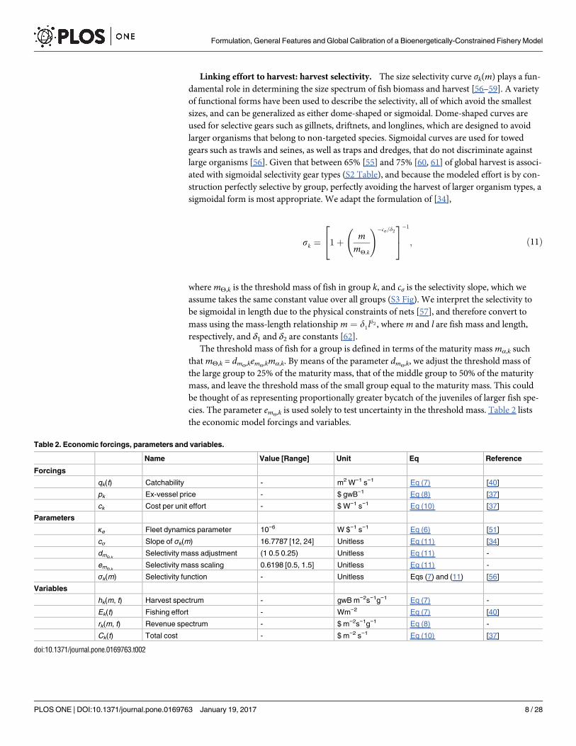
Linking effort to harvest: harvest selectivity. The size selectivity curve σk(m) plays a fun-damental role in determining the size spectrum of fish biomass and harvest [56–59]. A varietyof functional forms have been used to describe the selectivity, all of which avoid the smallestsizes, and can be generalized as either dome-shaped or sigmoidal. Dome-shaped curves areused for selective gears such as gillnets, driftnets, and longlines, which are designed to avoidlarger organisms that belong to non-targeted species. Sigmoidal curves are used for towedgears such as trawls and seines, as well as traps and dredges, that do not discriminate againstlarge organisms [56]. Given that between 65% [55] and 75% [60, 61] of global harvest is associ-ated with sigmoidal selectivity gear types (S2 Table), and because the modeled effort is by con-struction perfectly selective by group, perfectly avoiding the harvest of larger organism types, asigmoidal form is most appropriate. We adapt the formulation of [34],

sk à 1á mmY;k

!�cs=d224

35�1

; Ö11Ü

where mΘ,k is the threshold mass of fish in group k, and cσ is the selectivity slope, which weassume takes the same constant value over all groups (S3 Fig). We interpret the selectivity tobe sigmoidal in length due to the physical constraints of nets [57], and therefore convert to

mass using the mass-length relationship m à d1ld2 , where m and l are fish mass and length,respectively, and δ1 and δ2 are constants [62].

The threshold mass of fish for a group is defined in terms of the maturity mass mα,k suchthat mΘ,k = dmΘ,kemΘ,kmα,k. By means of the parameter dmΘ,k, we adjust the threshold mass ofthe large group to 25% of the maturity mass, that of the middle group to 50% of the maturitymass, and leave the threshold mass of the small group equal to the maturity mass. This couldbe thought of as representing proportionally greater bycatch of the juveniles of larger fish spe-cies. The parameter emΘ,k is used solely to test uncertainty in the threshold mass. Table 2 liststhe economic model forcings and variables.

Table 2. Economic forcings, parameters and variables.

Name Value [Range] Unit Eq Reference

Forcings

qk(t) Catchability - m2 W−1 s−1 Eq (7) [40]

pk Ex-vessel price - $ gwB−1 Eq (8) [37]

ck Cost per unit effort - $ W−1 s−1 Eq (10) [37]

Parameters

κe Fleet dynamics parameter 10−6 W $−1 s−1 Eq (6) [51]

cσ Slope of σk(m) 16.7787 [12, 24] Unitless Eq (11) [34]

dmΘ,kSelectivity mass adjustment (1 0.5 0.25) Unitless Eq (11) -

emΘ,kSelectivity mass scaling 0.6198 [0.5, 1.5] Unitless Eq (11) -

σk(m) Selectivity function - Unitless Eqs (7) and (11) [56]

Variables

hk(m, t) Harvest spectrum - gwB m−2s−1g−1 Eq (7) -

Ek(t) Fishing effort - Wm−2 Eq (7) [40]

rk(m, t) Revenue spectrum - $ m−2s−1g−1 Eq (8) -

Ck(t) Total cost - $ m−2 s−1 Eq (10) [37]




Assessment of parameter uncertainty and calibration

In order to evaluate uncertain model parameter values, we compare model simulations withtwo primary sources of global data. The first is stock assessment data as compiled in the RAMLegacy database [63]. These data provide an estimate of fish biomass, which is extremely use-ful; however, for most ecosystems, the stock assessments do not include the entirety of har-vested species, limiting their comparability to BOATS. Therefore, we also make use of globalcatch data, described in greater detail below, as reconstructed by the Sea Around Us Project(SAUP) [60, 61].

Because the harvest depends on economic as well as ecological forcings, there are multipleeconomic and ecological combinations that can produce the same harvest in a given region.On its own, this could lead to an intractable problem, with too many degrees of freedom. How-ever, we can take advantage of the fact that there is a maximum rate of fish production that anecosystem can achieve at any given location. Because of the historical increase of fishing inten-sity, most ecosystems are presently either close to this peak value (fully exploited), or havepassed it and gone into decline (over-exploited) or collapse [64]. We identify the observed

maximum multi-year harvest for each LME (which we denote as lHobsLMEmax, where l = 1, . . ., 66

is an index for the LMEs) as an estimate of the peak fish that can be produced by the ecosystemwhen subjected to a transient increase of fishing intensity. Although most of these estimateswill individually include uncertainties on the order of a factor of two, arising from uncertaintyin catch reconstructions [65], the large number of LMEs and their global distribution shouldprovide sufficient sampling to compensate these errors.

To evaluate the full uncertainty range of model parameters, including interactions betweenthe parameters, we used a Monte Carlo approach [66]. This involved first determining a proba-bility distribution for each parameter of interest, and then randomly generating over 10,000values for each parameter from each distribution (Fig 2). In order to compare with the

observed harvest peaks, lHobsLMEmax, we ran a transient simulation for each parameter combina-

tion, gradually increasing catchability over 200 years. In the following, we describe the simula-tions, the data, and the comparison between them.

Transient simulations with increasing catchability. The parameters considered in theMonte Carlo simulations are presented in Table 3, and further detailed in S1 Table. We con-sider the parameters that have the strongest influence on model biomass, as detailed in the fulldescription of the ecological module [24]. For each parameter, we reviewed the literature forstatistically-estimated ranges of values and their probability distributions. When such a statisti-cal range was not available, we used the literature to inform the parameter choices assuming auniform probability distribution.

For each parameter set, we first spin up the model with a 100-year simulation at a low andconstant level of catchability (1 × 10−5 m2 W−1 s−1), which is designed to result in negligibleharvests that are consistent with that set of parameters. To span an appropriate range of catch-ability values, following the first 100 years of constant catchability, we increase catchability by5% per year for 200 years. This rate of increase ensures that each simulation will produce apeak harvest under all parameter combinations, and is broadly consistent with estimates oftechnological increase [53].

Observational data. Under intense harvest, the harvest to biomass ratio reflects the abilityof a standing stock to produce harvestable biomass each year. We obtained harvest and bio-mass data from the RAM Legacy stock assessment database [63], and used them to calculateharvest to biomass ratios (H:B hereafter). Stock assessments, by their nature, target individualspecies in particular geographic regions. Because BOATS represents all commercial species, itsresults can only be compared with stock assessments when they represent a significant fraction



Fig 2. Schematic diagram of the Monte Carlo simulation procedure and selection of ensemble members.


Table 3. Monte Carlo simulation parameter summary results. MC Distribution is the sampling distribution of each parameter used in the Monte Carlo simu-lation, whereX (p1, p2) represents the probability distribution (N for normal, U for uniform), and p1 and p2 represent the mean and standard deviation of theparameter, respectively. Opt. refers to the subset of optimized Monte Carlo simulations, N.O. to the subset of non-optimized simulations, SD refers to the stan-dard deviation, and KS p-value is the p-value of the 2-sample Kolmogorov-Smirnov test applied to the optimized and non-optimized sets.

Parameter Name Sampling Distribution Mean Opt. Mean N.O. SD Opt. SD N.O. KS p-value

ωa,A Growth activation energy N (0.45, 0.09) 0.41 0.44 0.08 0.09 2.77 × 10−4

ωa,λ Mortality activation energy N (0.45, 0.09) 0.47 0.45 0.08 0.09 0.05

b Allometric scaling exponent U(0.7, 0.05) 0.65 0.70 0.03 0.05 1.47 × 10−16

A0 Allometric growth constant N (0.46, 0.5) 4.42 4.47 0.48 0.50 0.18

α Trophic efficiency U(0.13, 0.04) 0.15 0.13 0.03 0.04 1.04 × 10−11

β Predator to prey mass ratio U(5000, 2500) 5484 4991 2357 2507 0.08

τ Trophic scaling log(α)/log(β) −0.22 −0.25 0.02 0.04 5.27 × 10−17

kE Eppley constant N (0.0631, 0.009) 0.06 0.06 0.01 0.01 0.34

Π* Nutrient concentration N (0.37, 0.1) 0.35 0.37 0.09 0.10 0.06

ζ1 Mortality constant N (0.55, 0.57) 0.01 0.55 0.40 0.57 9.48 × 10−18

h Allometric mortality scaling N (0.54, 0.09) 0.49 0.54 0.08 0.09 4.39 × 10−5

se Egg survival fraction U(0.025, 0.014) 0.02 0.03 0.01 0.01 0.22

emΘ,k Selectivity position scaling U(1, 0.288) 0.88 1.00 0.29 0.29 8.89 × 10−7

cσ Selectivity slope U(18, 3.46) 17.8 18.0 3.46 3.47 0.84




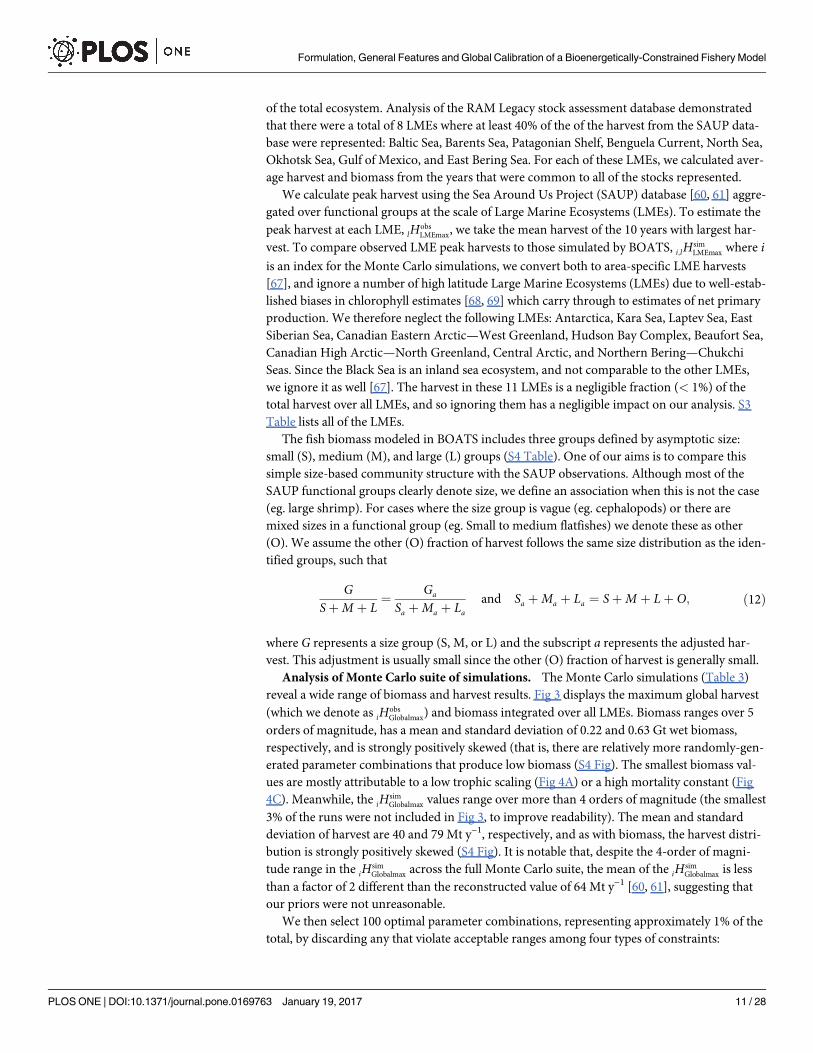
of the total ecosystem. Analysis of the RAM Legacy stock assessment database demonstratedthat there were a total of 8 LMEs where at least 40% of the of the harvest from the SAUP data-base were represented: Baltic Sea, Barents Sea, Patagonian Shelf, Benguela Current, North Sea,Okhotsk Sea, Gulf of Mexico, and East Bering Sea. For each of these LMEs, we calculated aver-age harvest and biomass from the years that were common to all of the stocks represented.

We calculate peak harvest using the Sea Around Us Project (SAUP) database [60, 61] aggre-gated over functional groups at the scale of Large Marine Ecosystems (LMEs). To estimate the

peak harvest at each LME, lHobsLMEmax, we take the mean harvest of the 10 years with largest har-

vest. To compare observed LME peak harvests to those simulated by BOATS, i;lHsimLMEmax where i

is an index for the Monte Carlo simulations, we convert both to area-specific LME harvests[67], and ignore a number of high latitude Large Marine Ecosystems (LMEs) due to well-estab-lished biases in chlorophyll estimates [68, 69] which carry through to estimates of net primaryproduction. We therefore neglect the following LMEs: Antarctica, Kara Sea, Laptev Sea, EastSiberian Sea, Canadian Eastern Arctic—West Greenland, Hudson Bay Complex, Beaufort Sea,Canadian High Arctic—North Greenland, Central Arctic, and Northern Bering—ChukchiSeas. Since the Black Sea is an inland sea ecosystem, and not comparable to the other LMEs,we ignore it as well [67]. The harvest in these 11 LMEs is a negligible fraction (< 1%) of thetotal harvest over all LMEs, and so ignoring them has a negligible impact on our analysis. S3Table lists all of the LMEs.

The fish biomass modeled in BOATS includes three groups defined by asymptotic size:small (S), medium (M), and large (L) groups (S4 Table). One of our aims is to compare thissimple size-based community structure with the SAUP observations. Although most of theSAUP functional groups clearly denote size, we define an association when this is not the case(eg. large shrimp). For cases where the size group is vague (eg. cephalopods) or there aremixed sizes in a functional group (eg. Small to medium flatfishes) we denote these as other(O). We assume the other (O) fraction of harvest follows the same size distribution as the iden-tified groups, such that

GSáM á L

à Ga

Sa áMa á Laand Sa áMa á La à SáM á Lá O; Ö12Ü

where G represents a size group (S, M, or L) and the subscript a represents the adjusted har-vest. This adjustment is usually small since the other (O) fraction of harvest is generally small.

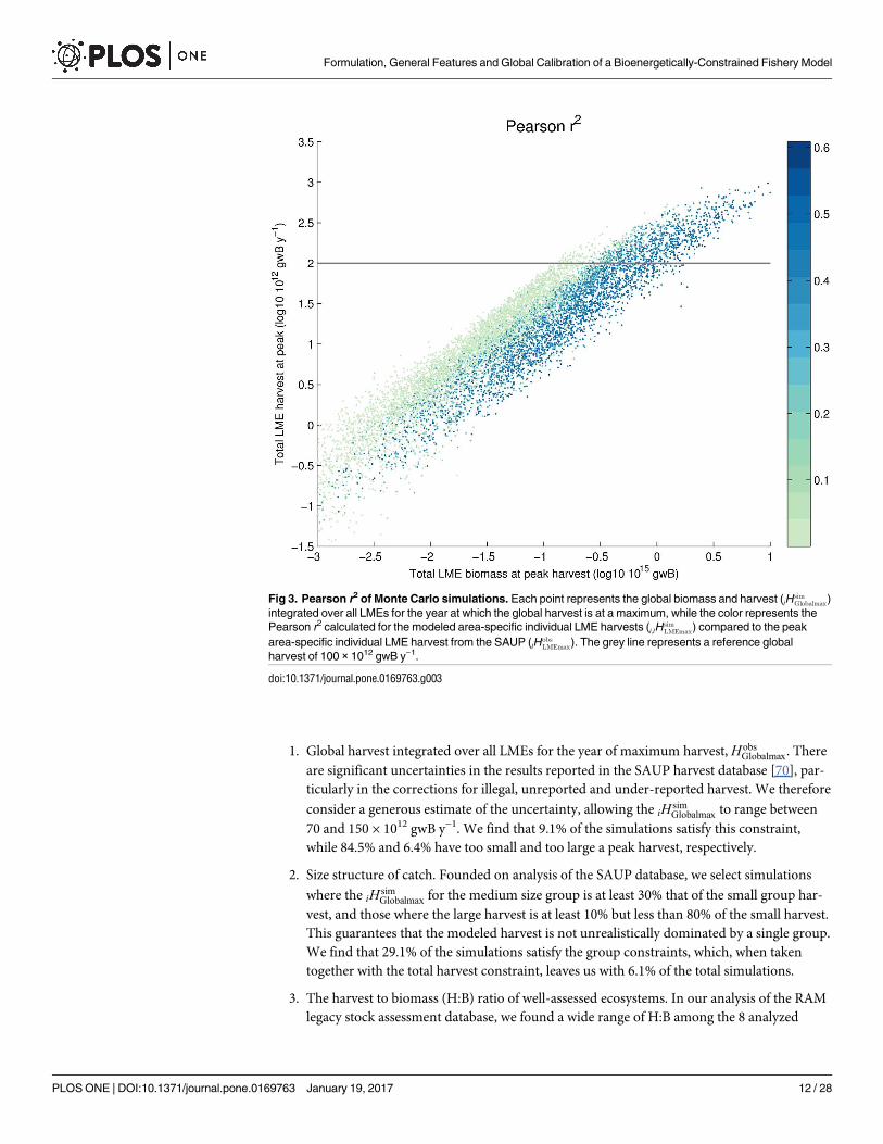
Analysis of Monte Carlo suite of simulations. The Monte Carlo simulations (Table 3)reveal a wide range of biomass and harvest results. Fig 3 displays the maximum global harvest

(which we denote as iHobsGlobalmax) and biomass integrated over all LMEs. Biomass ranges over 5

orders of magnitude, has a mean and standard deviation of 0.22 and 0.63 Gt wet biomass,respectively, and is strongly positively skewed (that is, there are relatively more randomly-gen-erated parameter combinations that produce low biomass (S4 Fig). The smallest biomass val-ues are mostly attributable to a low trophic scaling (Fig 4A) or a high mortality constant (Fig4C). Meanwhile, the iHsim

Globalmax values range over more than 4 orders of magnitude (the smallest

3% of the runs were not included in Fig 3, to improve readability). The mean and standarddeviation of harvest are 40 and 79 Mt y−1, respectively, and as with biomass, the harvest distri-bution is strongly positively skewed (S4 Fig). It is notable that, despite the 4-order of magni-tude range in the iHsim

Globalmax across the full Monte Carlo suite, the mean of the iHsimGlobalmax is less

than a factor of 2 different than the reconstructed value of 64 Mt y−1 [60, 61], suggesting thatour priors were not unreasonable.

We then select 100 optimal parameter combinations, representing approximately 1% of thetotal, by discarding any that violate acceptable ranges among four types of constraints:



1. Global harvest integrated over all LMEs for the year of maximum harvest,HobsGlobalmax. There

are significant uncertainties in the results reported in the SAUP harvest database [70], par-ticularly in the corrections for illegal, unreported and under-reported harvest. We therefore

consider a generous estimate of the uncertainty, allowing the iH simGlobalmax to range between

70 and 150 × 1012 gwB y−1. We find that 9.1% of the simulations satisfy this constraint,while 84.5% and 6.4% have too small and too large a peak harvest, respectively.

2. Size structure of catch. Founded on analysis of the SAUP database, we select simulations

where the iH simGlobalmax for the medium size group is at least 30% that of the small group har-

vest, and those where the large harvest is at least 10% but less than 80% of the small harvest.This guarantees that the modeled harvest is not unrealistically dominated by a single group.We find that 29.1% of the simulations satisfy the group constraints, which, when takentogether with the total harvest constraint, leaves us with 6.1% of the total simulations.

3. The harvest to biomass (H:B) ratio of well-assessed ecosystems. In our analysis of the RAMlegacy stock assessment database, we found a wide range of H:B among the 8 analyzed

Fig 3. Pearson r2 of Monte Carlo simulations. Each point represents the global biomass and harvest (iHsimGlobalmax)

integrated over all LMEs for the year at which the global harvest is at a maximum, while the color represents thePearson r2 calculated for the modeled area-specific individual LME harvests (i;lH

simLMEmax) compared to the peak

area-specific individual LME harvest from the SAUP (lHobsLMEmax). The grey line represents a reference global

harvest of 100 × 1012 gwB y−1.




Fig 4. Summary results of Monte Carlo simulations. Horizontal and vertical axes as in Fig 3. Circle colorrepresents (A) Trophic scaling τ, (B) Allometric growth scaling constant b, or (C) Mortality constant ζ1. Thegrey line represents a reference global harvest of 100 × 1012 gwB y−1.




LMEs, but in all cases, it was less than 0.4 y−1. We apply this constraint by calculating the

modeled H:B at peak harvest (i;lH simLMEmax) at each of the 8 LMEs. 74.2% of the Monte Carlo

simulations satisfy this H:B constraint when applied to the 8 LMEs. Taken together with theprior two constraints, we arrive at 3.9% of the simulations. Although there is great potentialto use improved stock assessment data in the future, for the present work we only apply theupper limit on the feasible H:B of these 8 LMEs.

4. The relative productivity of LMEs. We rank the remaining simulations by calculating the

correlation between the modeled peak harvest of each LME (i;lH simLMEmax) and the recon-

structed peak LME harvest from the SAUP (lHobsLMEmax). Because the LMEs span a wide

range of NPP and temperature, analyzing the simulated distribution of harvest among theLMEs provides a powerful means by which to evaluate model sensitivity to these two criticalinput variables. We consider the Pearson product-moment correlation coefficient r (plottedas r2), of the harvest per unit area in each LME, but also the log10 transformed harvest perunit area [67] (not shown), as well as Spearman’s rank correlation rs. We find a wide rangeof correlation values from among the members of the Monte Carlo suite, but there are clearpatterns of improving correlation with increasing biomass within the range of acceptableharvest which is consistent over the three correlation techniques considered (Fig 3). Fromamong the simulations with acceptable total harvest, the r2 ranges from close to zero to0.59, whereas Spearman’s rs ranges from −0.42 to 0.76. We select the best-correlated 1% ofthe total simulations, corresponding to an r2 larger than 0.45.

Table 3 summarizes the results of the analysis, and presents the mean of the optimized (col-umn Mean Opt.) and non-optimized (column Mean N.O.) parameter values, as well as theirstandard deviations (columns SD Opt. and SD N.O.). Fig 5 shows the transient time series oftotal LME fish biomass, harvest, and effort for the optimized set. Total LME harvest steadilyincreases until it reaches a peak, beyond which a sufficient portion of the global ocean becomesrecruitment-limited and harvest begins to fall. All simulations show a monotonic decrease ofbiomass as catchability increases, since the selectable biomass is progressively reduced towardsa limit, the critical biomass, that is discussed in the next section. This occurs in an increasingnumber of grid cells as greater catchability allows fishing to become profitable. Effort followsthe same general pattern as harvest, but consistently lags it. The timescale of biomass and effortchange is set mostly by the timescale of technology change, yet effort also responds with thetimescale of adjustment to revenue changes (the fleet dynamics parameter κe) which delays thechange of effort relative to biomass and harvest changes (Eq (13)). We overlay the optimizedensemble of simulated harvests in Fig 5B with two versions of the reconstructed SAUP harvest(black line [60, 61], red line [71]), assuming that year 1950 of the SAUP harvest corresponds toyear 100 of the 300-year transient simulation (when catchability begins to increase). Bothreconstructions show the same general trend as the simulated transient simulations over thehistorical period, and the red line (which attempts to correct for illegal and unreported catch)is close to the median of the simulations. Although the highest simulated values are possiblyover-estimates of the global potential fish production, it is useful to include these variants inthe ensemble given that their parameter combinations may represent aspects of the ecosystemsrealistically, even though they allow too much harvest.

Results and Discussion

The critical fish biomass

In considering the fundamental dynamics that arise from the BOATS formulation, we arrive ata useful observation regarding the equilibrium solution of Eq (6) for the evolution of effort.



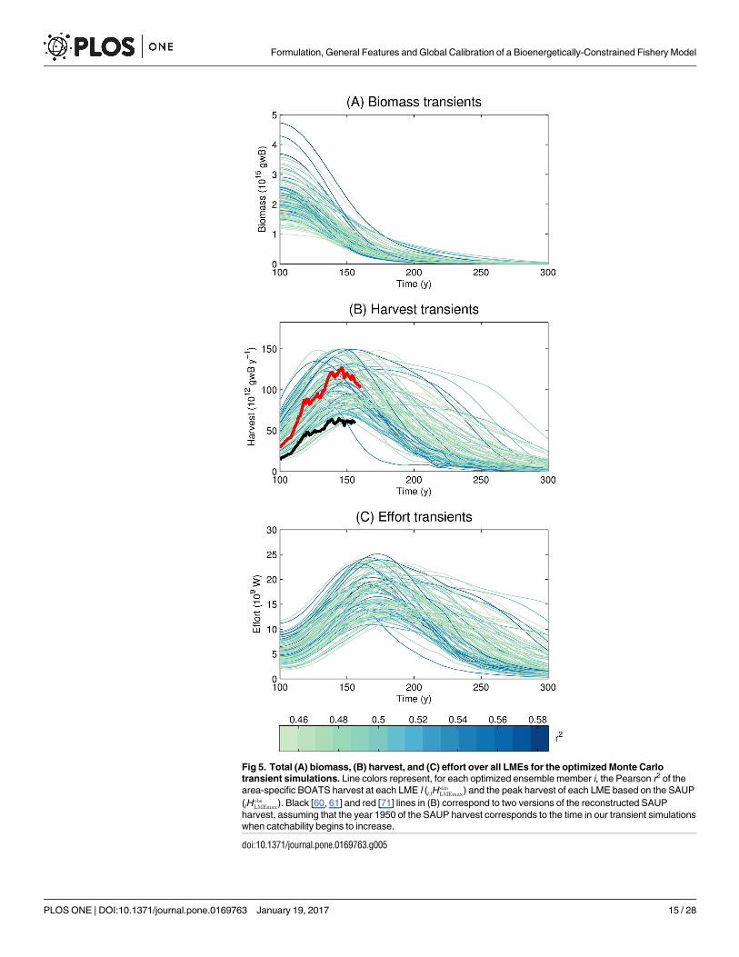
Fig 5. Total (A) biomass, (B) harvest, and (C) effort over all LMEs for the optimized Monte Carlotransient simulations. Line colors represent, for each optimized ensemble member i, the Pearson r2 of thearea-specific BOATS harvest at each LME l (i;lH

simLMEmax) and the peak harvest of each LME based on the SAUP

(lHobsLMEmax). Black [60, 61] and red [71] lines in (B) correspond to two versions of the reconstructed SAUP

harvest, assuming that the year 1950 of the SAUP harvest corresponds to the time in our transient simulationswhen catchability begins to increase.




We begin with the equations for revenue and cost, Eqs (9) and (10), respectively, and applythem to Eq (6) to find that

ddt

Ek à ke qk

Z m1;k

m0

pkskfkdm� ck

!: Ö13Ü

Further assuming that price does not depend on mass, we can write the equilibrium solutionof Eq (13) as Z m1;k

m0

skfkdm à ck

pkqkà Fcrit

k : Ö14Ü

This states that the selectable biomass (the quantity on the left hand side) of group k is, atsteady state, determined solely by the ratio of economic parameters, ck/pkqk. This ratio can alsobe interpreted as a critical threshold, which we refer to as Fcrit

k , which determines the biomass

density that is required at any given grid point in order for harvest to be profitable. If the equi-librium biomass ignoring harvest is less than Fcrit

k , then harvest cannot be profitable and there

will be no harvest at equilibrium. In this case, the biomass will be controlled by primary pro-duction and temperature, by means of Eq (1). Alternatively, if the selectable group biomassexceeds Fcrit

k , harvest will occur, driving the selectable biomass to asymptotically approach Fcritk ,

while the unselectable portion of the biomass will continue to be driven by primary productionand temperature.

The exclusive dependence of Fcritk on economic parameters is an important consequence of

the open access assumption used in the present version of the BOATS model. Although itwould not be expected to hold true in the real world, given for example the movement of fish,multi-species fisheries, and the lack of steady-state, it is a useful simplifying concept forexplaining the first-order tendencies of fish biomass in the absence of effective management.

General characteristics of the optimized bio-economic model

In order to illustrate the basic characteristics of the coupled model, we use the parameter com-bination that gives the highest correlation (r2) between modeled and observed harvests at thescale of LMEs. While we initially focus on results with this single set of model parameters forclarity, it is preferable to use an ensemble of optimal models, in order to better span theuncertainty.

The predictive ability of this model variant can be assessed by comparing the correlation ofthe SAUP harvest with the primary production used to force the model (Fig 6A), the simulatedunharvested LME biomass by LME (Fig 6B), and the modeled harvest (Fig 6C). We find thatNPP alone explains 32% of the variability in the SAUP harvest, similar to prior works [72],while unharvested model biomass explains 54%, and modeled harvest explains 59%. All corre-lations have a p-value<0.01. Thus, the inclusion of the interactive economics provides animprovement to the prediction of harvest, even though it did not introduce additional parame-ters into the optimization procedure.

Fig 7 illustrates some aspects of the model by focusing on a single model grid point in theEast Bering Sea LME (64˚N, 165˚W). A detailed description of the ecological model at this siteis provided in [24], and showed that the slope of modeled biomass spectra is consistent withobservations for a wide range of temperature and NPP values. Here, harvest alters the slopeand intercept of biomass spectra (Fig 7A), truncating the large ends of the spectra, consistentwith other modeling studies [73]. The truncation occurs because larger fish must grow fromsmaller fish, and so larger fish are affected both by direct harvesting and the reduction in



Fig 6. SAUP reconstructed harvest as described by primary production, modelled unharvestedbiomass, and modelled harvest at the LME scale. Correlations are for the model variant from the MonteCarlo simulation that best represents the SAUP database. The circle color represents the averagetemperature of the LME, whereas the number represents the LME number (S3 Table). All quantities areplotted in log10 space to improve readability. r2 is the squared Pearson product-moment correlationcoefficient, and rs is Spearman’s rank correlation. All 6 correlations have a p-value<0.01. (A) NPP vs. SAUPharvest. (B) Modelled unharvested biomass vs. SAUP harvest. (C) Modelled harvest at peak harvest state vs.SAUP harvest. The black line is the identity line (1:1 line).




Fig 7. Steady state biomass (A) and harvest (B) size spectra. Black solid, dashed, and dot-dashed curvesrepresent unharvested small, medium, and large groups, respectively, whereas grey curves representharvested spectra. Thick curves represent total biomass and harvest spectra. Curves are equilibriumsolutions of simulations for a site in the East Bering Sea LME (64˚N, 165˚W) forced with annual average netprimary production and temperature using a timestep of 15 days.




growth from smaller fish. Moreover, the loss of large, spawning individuals results in a reducedproduction of eggs and so a reduction in recruitment (Eq (5)) and juvenile biomass. Harvestspeak near the threshold size mΘ (Fig 7B), and decline both at smaller sizes (because of sharplydecreasing selectivities), and at larger sizes (because of rapidly decreasing biomasses andgrowth rates).

It is worth noting that, at low harvest and high biomass, the input energy from the transferof primary production to fish ξP (Eq (2)) is partitioned across a larger number of individual,and is generally the limiting factor for growth. On the other hand, at high harvest and low bio-mass, the same energy from primary production is partitioned to a smaller number of individ-uals, increasing their potential growth rates, to the point at which growth becomes limited bythe maximum physiological rate, expressed by ξVB. Thus, all else being equal, increasing har-vest and decreasing biomass determines a transition from productivity-limited to physiologi-cally-limited growth in the model.

Fig 8 illustrates the impact of NPP (ranging from 500 to 3000 mg C m−2 d−1) and catchabil-ity (ranging from 10−5 to 10−3 m2 W−1 s−1) on biomass and harvest. Each harvest (Fig 8A) andfraction of prisitine biomass remaining (Fig 8B) value is the equilibrium result of a 1000-yearsimulation using a 15-day timestep and constant forcing of annually-averaged NPP and tem-perature. For low catchability and low NPP (and hence low unharvested biomass), harvest iszero (0.01 gwB m−2 y−1 contour in Fig 8A) because the fishery is not profitable (Eq (14)). Withincreasing catchability or increasing NPP, we eventually surpass the Fcrit

k limit for a profitable

fishery, and arrive at positive harvest. For a given level of NPP, increasing catchability initiallyresults in rising harvest, until the peak is reached, after which further increases of catchabilitydeplete the ability of the population to produce biomass due to stock-limitation of recruitment[74]. As a result, there is a peak equilibrium harvest for every value of NPP. For high catchabil-ity, both harvest and the fraction of pristine biomass approach zero (0.01 gwB m−2 y−1 and0.001 contours at the right of Fig 8A and 8B, respectively).

Insights on uncertain parameters

We use the two-sample Kolmogorov-Smirnov test (Table 3, column KS p-value) to comparethe distributions of the optimized and non-optimized parameters to determine if they are gen-erated from the same distribution ([75], p. 428-441). For 7 parameters, we find no differencein the distributions that generate the optimized and non-optimized simulations. However, forthe remaining 6 parameters, there is a clear statistical difference (that is, small p-values). Prom-inent differences are in the mortality parameters z1 (Fig 4C) and h, that have significantlylower means and standard deviations. The difference between the optimized and non-opti-mized mortality rate z1 is particularly strong. This indicates that, in our model, only the lowerrange of possible mortality rates [26] can reproduce the present-day global peak harvest distri-butions. The optimized mean value of the allometric scaling parameter, b, which we assumefollows a uniform distribution ranging from 0.61 to 0.78, is 0.65, that is, indistinguishablefrom the 2/3 value that is widely used in the literature [76], but somewhat smaller than the0.75–0.79 value of other studies [25, 77]. We also find a preferred trophic efficiency of 0.15, sta-tistically higher than that of the sampling distribution, and encouragingly close to the value of0.15 that is widely applied. The activation energy of metabolism for mortality, ωa,λ, is not sta-tistically different from the sampling distribution, but that for growth ωa,A is, with a statisticallysignificant lower mean. This lends support to the idea that growth and mortality rates are notsubject to the same temperature dependence [78], and suggests that mortality may be moresensitive to temperature variations than growth.



The ensemble optimization reveals that acceptable parameter combinations have significantcorrelations between some model parameters. Some of these correlations, including the twostrongest ones, are shown in Fig 9. The mortality constant, z1, and the allometric scaling ofmortality, h, are negatively correlated in the ensemble (Pearson correlation coefficient r =−0.82, p-value<0.01) and compensate each other so that a high mortality constant is balancedby a weak size-dependence (low h) of mortality (Fig 9A). We also find a positive correlation(r = 0.68, p-value<0.01) between the mortality constant and the trophic scaling (Fig 9B)

Fig 8. Model sensitivity to NPP and catchability q. (A) Total harvest and (B) Fraction of pristine biomassremaining as functions of NPP and q.




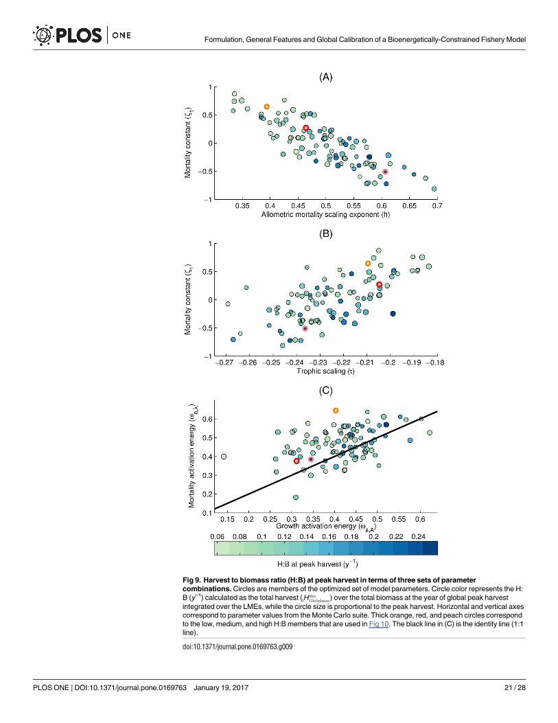
Fig 9. Harvest to biomass ratio (H:B) at peak harvest in terms of three sets of parametercombinations. Circles are members of the optimized set of model parameters. Circle color represents the H:B (y−1) calculated as the total harvest (iH

simGlobalmax) over the total biomass at the year of global peak harvest

integrated over the LMEs, while the circle size is proportional to the peak harvest. Horizontal and vertical axescorrespond to parameter values from the Monte Carlo suite. Thick orange, red, and peach circles correspondto the low, medium, and high H:B members that are used in Fig 10. The black line in (C) is the identity line (1:1line).




suggesting that higher mortalities can be balanced by increased energy transfer to large sizeclasses. Finally, we highlight a positive correlation (r = 0.41, p-value<0.01) between the activa-tion energies of growth and mortality (Fig 9C), which control the temperature dependence ofthese rates. This covariation indicates that, in order to maintain harvests in agreement withobservations, temperature-driven increases in mortality need to be balanced by concurrentincreases in growth rates. As noted above, the temperature dependence of mortality generallyexceeds the temperature dependence of growth, with 80% of the optimized ensemble lyingabove the 1:1 line.

Fig 9 also highlights the impact of several fundamental model parameters on simulated H:B. Low mortality constants, high allometric growth exponents, and high growth rate constantstend to occur with high H:B (r between z1, b, and A0, respectively, with H:B are −0.49, 0.65,and 0.30, p-value<0.01). Across the 105 members of the optimized Monte Carlo set, the H:Bcalculated for the global peak harvest (calculated by taking the ratio of total harvest over theLMEs, iHsim

Globalmax, to the total biomass over the LMEs) varies by approximately a factor of 5,

indicating that between 5 and 25% of the standing stock of biomass is harvested every year atthe peak. This range indicates that, within the limits allowed by the observational constraints,similar harvest can be sustained by substantially different levels of biomass.

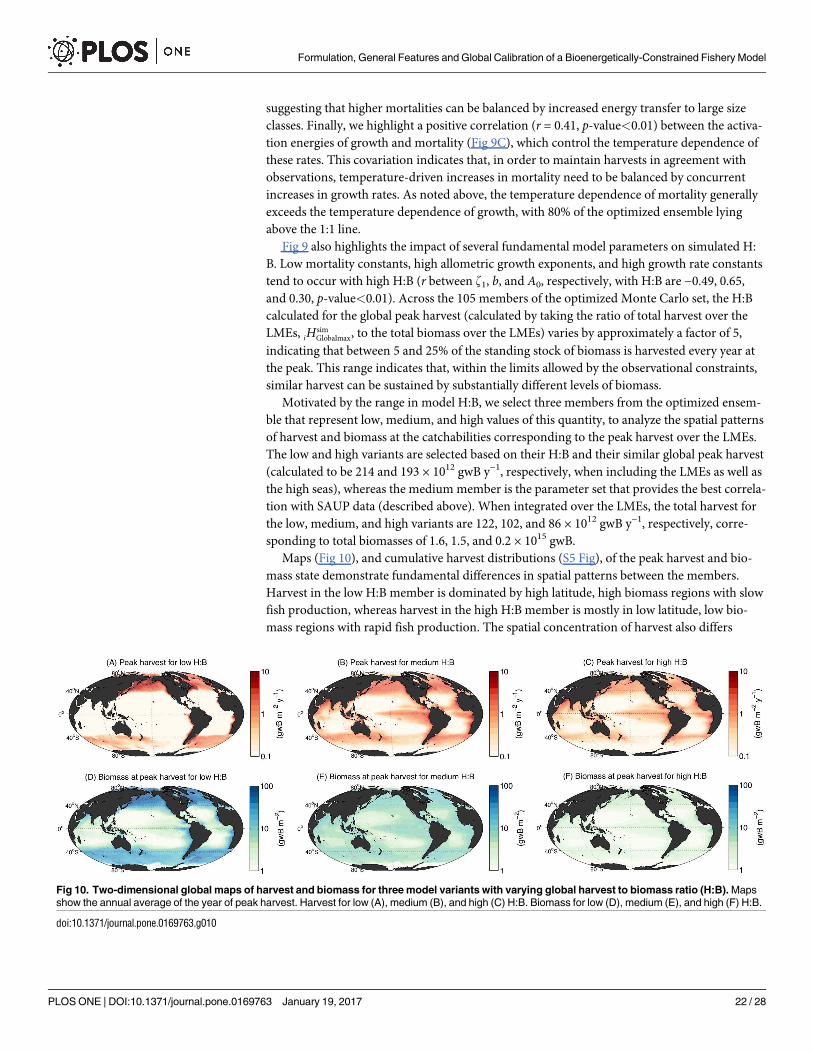
Motivated by the range in model H:B, we select three members from the optimized ensem-ble that represent low, medium, and high values of this quantity, to analyze the spatial patternsof harvest and biomass at the catchabilities corresponding to the peak harvest over the LMEs.The low and high variants are selected based on their H:B and their similar global peak harvest(calculated to be 214 and 193 × 1012 gwB y−1, respectively, when including the LMEs as well asthe high seas), whereas the medium member is the parameter set that provides the best correla-tion with SAUP data (described above). When integrated over the LMEs, the total harvest forthe low, medium, and high variants are 122, 102, and 86 × 1012 gwB y−1, respectively, corre-sponding to total biomasses of 1.6, 1.5, and 0.2 × 1015 gwB.

Maps (Fig 10), and cumulative harvest distributions (S5 Fig), of the peak harvest and bio-mass state demonstrate fundamental differences in spatial patterns between the members.Harvest in the low H:B member is dominated by high latitude, high biomass regions with slowfish production, whereas harvest in the high H:B member is mostly in low latitude, low bio-mass regions with rapid fish production. The spatial concentration of harvest also differs

Fig 10. Two-dimensional global maps of harvest and biomass for three model variants with varying global harvest to biomass ratio (H:B). Mapsshow the annual average of the year of peak harvest. Harvest for low (A), medium (B), and high (C) H:B. Biomass for low (D), medium (E), and high (F) H:B.




dramatically, with over 60% of harvest taking place at locations with high harvest rates (above3 gwB m−2 y−1) in the low H:B member, whereas harvest is much more widely distributed inthe high H:B member, with only about 25% of harvest taking place at location with high har-vest rates. Because of important differences in the model sensitivity to temperature (Fig 9C),contrasting projections of climate change impacts in low versus high latitude ecosystems [79],as well as potentially different resilience of low and high biomass conditions to overfishing, itwill be important to further constrain the uncertainty in H:B.

The significant variability of H:B among the 100-member ensemble arises in part from thegenerous ranges of observational uncertainty applied in the parameter optimization. Expand-ing and strengthening the observational constraints, for example from stock assessmentsaggregated at the LME scale, will further narrow the uncertainty in model parameters, andreduce the ensemble range of H:B. Future work should therefore strive to find stronger con-straints on harvest and biomass, such as by focusing on a subset of the best-studied LMEs.

Conclusion

The BOATS model represents the first-order features of global fish biomass and economic har-vest using fundamental concepts of macroecology, life-history, and resource economics in aunified spatially-resolved framework. The economic module of BOATS is directly coupled tothe biophysical model by means of the fishing effort, which responds dynamically to net profitsat the grid scale. Given the complex nature of real-world ecosystems and of the social and eco-nomic processes that determine fishing effort and harvest, the ability of BOATS to explain asignificant amount of the global spatial variability in harvest is promising, and makes it suitablefor exploratory global studies of fisheries dynamics that include both human and environmen-tal forcings.

A distinctive feature of this work is the use of a Monte Carlo approach to parse the uncer-tainty in the model parameters and to determine which parameter sets generate the best repre-sentations of present-day harvest from the Sea Around Us Project database. We find thatalthough most parameter combinations among the probability distributions of our priors areunable to produce the observed fish harvest, the central values of the distributions are associ-ated with a global harvest that is reasonably close to observations. By discarding unacceptableparameter combinations using a series of catch and biomass criteria, we arrive at an optimalensemble of about 100 parameter combinations that perform well, while still retaining a sub-stantial degree of parameter uncertainty. These optimal parameter combinations tend toinclude rates of natural mortality among the lower range of the sampling distribution, a resultthat deserves further attention given that natural mortality rates are difficult to constrain fromobservations. We also find that the temperature dependence of mortality is most often greaterthan the temperature dependence of fish growth, which has important implications in a warm-ing ocean. Realistic global harvests can be achieved by parameter combinations that result indifferent biomass distributions, and range from solutions dominated by slowly-growing abun-dant biomass in high latitudes and coastal regions, to solutions dominated by fast-growing lowbiomasses in low-latitudes and open-ocean waters. These remaining uncertainties allow apotential range of responses of the global fishery to human and climate-driven perturbations,which could be further narrowed down by considering improved biomass-based observationalconstraints.

Supporting Information

S1 Fig. Annual average net primary production (mg C m−2 d−1) forcing applied in BOATS.(PDF)



http://www.plosone.org/article/fetchSingleRepresentation.action?uri=info:doi/10.1371/journal.pone.0169763.s001

S2 Fig. Annual average 75-meter average temperature (˚C) forcing applied in BOATS.(PDF)

S3 Fig. Harvest selectivity σk by group.(PDF)

S4 Fig. Histograms of LME-integrated biomass and harvest from the Monte Carlo suite.(PDF)

S5 Fig. Cumulative fraction of global harvest integrated over all grid cells with a harvestrate less than a threshold harvest rate for low, medium, and high harvest to biomass ratio(H:B) model variants.(PDF)

S1 Table. Ecological model parameters.(PDF)

S2 Table. Gear types in terms of selectivity functional form (S = sigmoidal, G = gaussian,O = other) and percentage of global harvest (Table 3 of [55]).(PDF)

S3 Table. Large Marine Ecosystem numbers and names.(PDF)

S4 Table. Partitioning of SAUP functional groups into small (S), medium (M), large (L),and other (O) size groups.(PDF)

Acknowledgments

We acknowledge and thank the Sea Around Us Project; Pauly D. and Zeller D. (Editors), 2015.Sea Around Us Concepts, Design and Data (seaaroundus.org). We thank Ammar Adenwalafor assistance in analyzing the RAM Legacy Database, and thank Elizabeth Fulton for com-ments on an earlier version of this manuscript that were a part of the external review of DAC’sdoctoral thesis. Computational infrastructure was provided by the Canadian Foundation forInnovation (www.innovation.ca).

Author Contributions

Conceptualization: DAC DB EDG.

Data curation: DAC DB.

Formal analysis: DAC.

Funding acquisition: EDG DAC.

Investigation: DAC.

Methodology: DAC DB EDG.

Project administration: EDG.

Resources: EDG.

Software: DAC DB.

Supervision: EDG.











http://www.innovation.ca

Validation: DAC DB.

Visualization: DAC EDG.

Writing – original draft: DAC.

Writing – review & editing: DAC DB EDG.

References1. Watson RA, Cheung WWL, Anticamara JA, Sumaila RU, Zeller D, Pauly D. Global marine yield halved

as fishing intensity redoubles. Fish and Fisheries. 2013; 14(4):493–503. doi: 10.1111/j.1467-2979.2012.00483.x

2. Myers RA, Worm B. Rapid worldwide depletion of predatory fish communities. Nature. 2003; 423(6937):280–283. doi: 10.1038/nature01610 PMID: 12748640

3. McCauley DJ, Pinsky ML, Palumbi SR, Estes JA, Joyce FH, Warner RR. Marine defaunation: Animalloss in the global ocean. Science. 2015; 347(6219):1255641. doi: 10.1126/science.1255641 PMID:25593191

4. Mullon C, Freon P, Cury P. The dynamics of collapse in world fisheries. Fish and Fisheries. 2005; 6(2):111–120. doi: 10.1111/j.1467-2979.2005.00181.x

5. Branch TA, Jensen OP, Ricard D, YE Y, Hilborn R. Contrasting global trends in marine fishery statusobtained from catches and from stock assessments. Conservation Biology. 2011;

6. Doney SC, Ruckelshaus M, Emmett Duffy J, Barry JP, Chan F, English CA, et al. Climate ChangeImpacts on Marine Ecosystems. Annual Review of Marine Science. 2012; 4(1):11–37. doi: 10.1146/annurev-marine-041911-111611 PMID: 22457967

7. Pinsky ML, Worm B, Fogarty MJ, Sarmiento JL, Levin SA. Marine Taxa Track Local Climate Velocities.Science. 2013; 341(6151):1239–1242. doi: 10.1126/science.1239352 PMID: 24031017

8. Poloczanska ES, Brown CJ, Sydeman WJ, Kiessling W, Schoeman DS, Moore PJ, et al. Global imprintof climate change on marine life. Nature Climate Change. 2013; 3(10):919–925. doi: 10.1038/nclimate1958

9. Brander K. Impacts of climate change on fisheries. Journal of Marine Systems. 2010; 79(3-4):389–402.doi: 10.1016/j.jmarsys.2008.12.015

10. Sumaila UR, Cheung WWL, Lam VWY, Pauly D, Herrick S. Climate change impacts on the biophysicsand economics of world fisheries. Nature Climate Change. 2011; 1(9):449–456. doi: 10.1038/nclimate1301

11. Squires D, Vestergaard N. Technical Change and The Commons. Review of Economics and Statistics.2013; 95(5):1769–1787. doi: 10.1162/REST_a_00346

12. Mullon C, Guillotreau P, Galbraith ED, Fortilus J, Chaboud C, Bopp L, et al. Exploring future scenariosfor the global supply chain of tuna. Deep Sea Research Part II: Topical Studies in Oceanography. 2016;p. –.

13. Fulton EA. Approaches to end-to-end ecosystem models. Journal of Marine Systems. 2010; 81:171–183. doi: 10.1016/j.jmarsys.2009.12.012

14. Griffith GP, Fulton EA. New approaches to simulating the complex interaction effects of multiple humanimpacts on the marine environment. ICES Journal of Marine Science. 2014; 71(4):764–774. doi: 10.1093/icesjms/fst196

15. Kearney KA, Stock C, Aydin K, Sarmiento JL. Coupling planktonic ecosystem and fisheries food webmodels for a pelagic ecosystem: Description and validation for the subarctic Pacific. Ecological Model-ling. 2012; 237-238:43–62. doi: 10.1016/j.ecolmodel.2012.04.006

16. Jørgensen C, Enberg K, Dunlop ES, Arlinghaus R, Boukal DS, Brander K, et al. Ecology: ManagingEvolving Fish Stocks. Science. 2007; 318(5854):1247–1248. doi: 10.1126/science.1148089 PMID:18033868

17. Maury O, Faugeras B, Shin YJ, Poggiale JC, Ben Ari T, Marsac F. Modeling environmental effects onthe size-structured energy flow through marine ecosystems. Part 1: The model. Progress in Oceanogra-phy. 2007; 74(4):479–499. doi: 10.1016/j.pocean.2007.05.002

18. Jennings S, Melin F, Blanchard JL, Forster RM, Dulvy NK, Wilson RW. Global-scale predictions of com-munity and ecosystem properties from simple ecological theory. Proceedings of the Royal Society B:Biological Sciences. 2008; 275(1641):1375–1383. doi: 10.1098/rspb.2008.0192 PMID: 18348964



http://dx.doi.org/10.1111/j.1467-2979.2012.00483.x

http://dx.doi.org/10.1111/j.1467-2979.2012.00483.x

http://dx.doi.org/10.1038/nature01610

http://www.ncbi.nlm.nih.gov/pubmed/12748640

http://dx.doi.org/10.1126/science.1255641


http://dx.doi.org/10.1111/j.1467-2979.2005.00181.x

http://dx.doi.org/10.1146/annurev-marine-041911-111611

http://dx.doi.org/10.1146/annurev-marine-041911-111611




http://dx.doi.org/10.1038/nclimate1958


http://dx.doi.org/10.1016/j.jmarsys.2008.12.015



http://dx.doi.org/10.1162/REST_a_00346

http://dx.doi.org/10.1016/j.jmarsys.2009.12.012

http://dx.doi.org/10.1093/icesjms/fst196

http://dx.doi.org/10.1093/icesjms/fst196

http://dx.doi.org/10.1016/j.ecolmodel.2012.04.006



http://dx.doi.org/10.1016/j.pocean.2007.05.002

http://dx.doi.org/10.1098/rspb.2008.0192


19. Cheung WWL, Lam VWY, Sarmiento JL, Kearney K, Watson R, Zeller D, et al. Large-scale redistribu-tion of maximum fisheries catch potential in the global ocean under climate change. Global Change Biol-ogy. 2010; 16(1):24–35. doi: 10.1111/j.1365-2486.2009.01995.x

20. Blanchard JL, Jennings S, Holmes R, Harle J, Merino G, Allen JI, et al. Potential consequences of cli-mate change for primary production and fish production in large marine ecosystems. PhilosophicalTransactions of the Royal Society B: Biological Sciences. 2012; 367(1605):2979–2989. doi: 10.1098/rstb.2012.0231 PMID: 23007086

21. Watson JR, Stock CA, Sarmiento JL. Exploring the role of movement in determining the global distribu-tion of marine biomass using a coupled hydrodynamic—Size-based ecosystem model. Progress inOceanography. 2014;

22. Jennings S, Collingridge K. Predicting Consumer Biomass, Size-Structure, Production, Catch Potential,Responses to Fishing and Associated Uncertainties in the World’s Marine Ecosystems. PLoS ONE.2015; 10(7):1–28. doi: 10.1371/journal.pone.0133794 PMID: 26226590

23. Christensen V, Coll M, Buszowski J, Cheung WWL, Frolicher T, Steenbeek J, et al. The global ocean isan ecosystem: simulating marine life and fisheries. Global Ecology and Biogeography. 2015; 24(5):507–517. doi: 10.1111/geb.12281

24. Carozza DA, Bianchi D, Galbraith ED. The ecological module of BOATS-1.0: a bioenergetically con-strained model of marine upper trophic levels suitable for studies of fisheries and ocean biogeochem-istry. Geoscientific Model Development. 2016; p. 1545–1565.

25. Brown JH, Gillooly JF, Allen AP, Savage VM, West GB. Toward a metabolic theory of ecology. Ecology.2004; 85(7):1771–1789. doi: 10.1890/03-9000

26. Gislason H, Daan N, Rice JC, Pope JG. Size, growth, temperature and the natural mortality of marinefish. Fish and Fisheries. 2010; 11(2):149–158. doi: 10.1111/j.1467-2979.2009.00350.x

27. Charnov EL, Gislason H, Pope JG. Evolutionary assembly rules for fish life histories. Fish and Fisheries.2012; 14(2):213–224. doi: 10.1111/j.1467-2979.2012.00467.x

28. Andersen KH, Beyer JE. Size structure, not metabolic scaling rules, determines fisheries referencepoints. Fish and Fisheries. 2013;

29. Lehodey P, Senina I, Murtugudde R. A spatial ecosystem and populations dynamics model (SEAPO-DYM) – Modeling of tuna and tuna-like populations. Progress in Oceanography. 2008; 78(4):304–318.doi: 10.1016/j.pocean.2008.06.004

30. McKendrick AG. Applications of mathematics to medical problems. Proceedings of the Edinburgh Math-ematical Society. 1926; 3:98–130. doi: 10.1017/S0013091500034428

31. von Foerster H. Some remarks on changing populations. In: Stohlman F Jr, editor. The Kinetics of Cellu-lar Proliferation. New York: Grune and Stratton; 1959.

32. Ernest SKM, Enquist BJ, Brown JH, Charnov EL, Gillooly JF, Savage VM, et al. Thermodynamic andmetabolic effects on the scaling of production and population energy use. Ecology Letters. 2003; 6(11):990–995. doi: 10.1046/j.1461-0248.2003.00526.x

33. von Bertalanffy L. Problems of Organic Growth. Nature. 1949; 163(4135):156–158. doi: 10.1038/163156a0 PMID: 18107581

34. Hartvig M, Andersen KH, Beyer JE. Food web framework for size-structured populations. Journal of the-oretical Biology. 2011; 272(1):113–122. doi: 10.1016/j.jtbi.2010.12.006 PMID: 21146543

35. Rothschild BJ. An exposition on the definition of fishing effort. Fishery Bulletin. 1972; 70(3):671–679.

36. Anticamara JA, Watson R, Gelchu A, Pauly D. Global fishing effort (1950–2010): Trends, gaps, andimplications. Fisheries Research. 2011; 107(1-3):131–136. doi: 10.1016/j.fishres.2010.10.016

37. Smith VL. Economics of production from natural resources. The American Economic Review. 1968; 58(3):409–431.

38. Branch TA, Hilborn R, Haynie AC, Fay G, Flynn L, Griffiths J, et al. Fleet dynamics and fishermenbehavior: lessons for fisheries managers. Canadian Journal of Fisheries and Aquatic Sciences. 2006;63(7):1647–1668. doi: 10.1139/f06-072

39. Gordon H Scott. The Economic Theory of a Common-Property Resource: The Fishery. Journal of Politi-cal Economy. 1954; 62(2):124–142. doi: 10.1086/257497

40. Schaefer MB. Some aspects of the dynamics of populations important to the management of the com-mercial marine fisheries. Bulletin of the Inter-American Tropical Tuna Commission. 1954; 1(2):27–56.

41. Clark CW. Mathematical Bioeconomics: The Optimal Management of Renewable Resources, SecondEdition. New York, NY, USA: John Wiley & Sons, Inc.; 1990.

42. Hardin G. The tragedy of the commons. The population problem has no technical solution; it requires afundamental extension in morality. Science. 1968; 162(859):1243. PMID: 5699198



http://dx.doi.org/10.1111/j.1365-2486.2009.01995.x

http://dx.doi.org/10.1098/rstb.2012.0231



http://dx.doi.org/10.1371/journal.pone.0133794


http://dx.doi.org/10.1111/geb.12281

http://dx.doi.org/10.1890/03-9000

http://dx.doi.org/10.1111/j.1467-2979.2009.00350.x

http://dx.doi.org/10.1111/j.1467-2979.2012.00467.x

http://dx.doi.org/10.1016/j.pocean.2008.06.004

http://dx.doi.org/10.1017/S0013091500034428

http://dx.doi.org/10.1046/j.1461-0248.2003.00526.x

http://dx.doi.org/10.1038/163156a0

http://dx.doi.org/10.1038/163156a0


http://dx.doi.org/10.1016/j.jtbi.2010.12.006


http://dx.doi.org/10.1016/j.fishres.2010.10.016

http://dx.doi.org/10.1139/f06-072

http://dx.doi.org/10.1086/257497


43. Dietz T, Ostrom E, Stern PC. The Struggle to Govern the Commons. Science. 2003; 302(5652):1907–1912. doi: 10.1126/science.1091015 PMID: 14671286

44. Wilen JE. Renewable Resource Economists and Policy: What Differences Have We Made? Journal ofEnvironmental Economics and Management. 2000; 39(3):306–327. doi: 10.1006/jeem.1999.1110

45. Caddy JF, Cochrane KL. A review of fisheries management past and present and some future perspec-tives for the third millennium. Ocean & coastal management. 2001; 44(9):653–682. doi: 10.1016/S0964-5691(01)00074-6

46. Costello C, Lynham J, Lester SE, Gaines SD. Economic Incentives and Global Fisheries Sustainability.Annual Review of Resource Economics. 2010; 2(1):299–318. doi: 10.1146/annurev.resource.012809.103923

47. Sumaila UR, Khan AS, Dyck AJ, Watson R, Munro G, Tydemers P, et al. A bottom-up re-estimation ofglobal fisheries subsidies. Journal of Bioeconomics. 2010; 12(3):201–225. doi: 10.1007/s10818-010-9091-8

48. Seijo J, Defeo O, Salas S. Fisheries bioeconomics. Theory, modelling and management. FAO FisheriesTechnical Paper, Rome, FAO. 1998;(368).

49. Holley JF, Marchal P. Fishing strategy development under changing conditions: examples from theFrench offshore fleet fishing in the North Atlantic. ICES Journal of Marine Science. 2004; 61(8):1410–1431. doi: 10.1016/j.icesjms.2004.08.010

50. Vermard Y, Marchal P, Mahevas S, Thebaud O. A dynamic model of the Bay of Biscay pelagic fleet sim-ulating fishing trip choice: the response to the closure of the European anchovy (Engraulis encrasicolus)fishery in 2005. Canadian Journal of Fisheries and Aquatic Sciences. 2008; 65(11):2444–2453. doi: 10.1139/F08-147

51. Rochet MJ, Daurès F, Trenkel VM, Walters C. Capacity management, not stock status or economics,drives fleet dynamics in the Bay of Biscay ecosystem on a decadal time scale. Canadian Journal ofFisheries and Aquatic Sciences. 2012; 69(4):695–710. doi: 10.1139/f2012-002

52. Arreguın-Sanchez F. Catchability: a key parameter for fish stock assessment. Reviews in Fish Biologyand Fisheries. 1996; 6(2):221–242. doi: 10.1007/BF00182344

53. Pauly D, Palomares MD. An empirical equation to predict annual increases in fishing efficiency. Fisher-ies Centre University of British Columbia, Working Paper Series 2010-07. 2010;.

54. Sethi SA, Branch TA, Watson R. Global fishery development patterns are driven by profit but not trophiclevel. Proceedings of the National Academy of Sciences. 2010; 107(27):12163–12167. doi: 10.1073/pnas.1003236107

55. Lam VWY, Sumaila UR, Dyck A, Pauly D, Watson R. Construction and first applications of a global costof fishing database. ICES Journal of Marine Science. 2011; 68(9):1996–2004. doi: 10.1093/icesjms/fsr121

56. Millar RB, Fryer RJ. Estimating the size-selection curves of towed gears, traps, nets and hooks.Reviews in Fish Biology and Fisheries. 1999; 9(1):89–116. doi: 10.1023/A:1008838220001

57. Rochet MJ, Collie JS, Jennings S, Hall SJ. Does selective fishing conserve community biodiversity?Predictions from a length-based multispecies model. Journal of the Fisheries Board of Canada. 2011;68(3):469–486.

58. Law R, Plank MJ, Kolding J. On balanced exploitation of marine ecosystems: results from dynamic sizespectra. ICES Journal of Marine Science. 2012; 69(4):602–614. doi: 10.1093/icesjms/fss031

59. Garcia SM, Kolding J, Rice J, Rochet MJ, Zhou S, Arimoto T, et al. Reconsidering the Consequences ofSelective Fisheries. Science. 2012; 335(6072):1045–1047. doi: 10.1126/science.1214594 PMID:22383833

60. Watson R, Revenga C, Kura Y. Fishing gear associated with global marine catches. FisheriesResearch. 2006; 79(1-2):97–102. doi: 10.1016/j.fishres.2006.01.013

61. Pauly D. The Sea Around Us Project: Documenting and Communicating Global Fisheries Impacts onMarine Ecosystems. AMBIO: A Journal of the Human Environment. 2007; 36(4):290–295. doi: 10.1579/0044-7447(2007)36%5B290:TSAUPD%5D2.0.CO;2

62. Froese R, Thorson JT, Reyes RB Jr. A Bayesian approach for estimating length-weight relationships infishes. Journal of Applied Ichthyology. 2013; 30(1):78–85. doi: 10.1111/jai.12299

63. Ricard D, Minto C, Jensen OP, Baum JK. Examining the knowledge base and status of commerciallyexploited marine species with the RAM Legacy Stock Assessment Database. Fish and Fisheries. 2011;13(4):380–398. doi: 10.1111/j.1467-2979.2011.00435.x

64. Hilborn R, Branch TA, Ernst B, Magnusson A, Minte-Vera CV, Scheuerell MD, et al. STATE OF THEWORLD’S FISHERIES. Annual Review of Environment and Resources. 2003; 28(1):359–399. doi: 10.1146/annurev.energy.28.050302.105509





http://dx.doi.org/10.1006/jeem.1999.1110

http://dx.doi.org/10.1016/S0964-5691(01)00074-6

http://dx.doi.org/10.1016/S0964-5691(01)00074-6

http://dx.doi.org/10.1146/annurev.resource.012809.103923

http://dx.doi.org/10.1146/annurev.resource.012809.103923

http://dx.doi.org/10.1007/s10818-010-9091-8

http://dx.doi.org/10.1007/s10818-010-9091-8

http://dx.doi.org/10.1016/j.icesjms.2004.08.010

http://dx.doi.org/10.1139/F08-147

http://dx.doi.org/10.1139/F08-147

http://dx.doi.org/10.1139/f2012-002

http://dx.doi.org/10.1007/BF00182344

http://dx.doi.org/10.1073/pnas.1003236107

http://dx.doi.org/10.1073/pnas.1003236107

http://dx.doi.org/10.1093/icesjms/fsr121

http://dx.doi.org/10.1093/icesjms/fsr121

http://dx.doi.org/10.1023/A:1008838220001

http://dx.doi.org/10.1093/icesjms/fss031




http://dx.doi.org/10.1579/0044-7447(2007)36%5B290:TSAUPD%5D2.0.CO;2

http://dx.doi.org/10.1579/0044-7447(2007)36%5B290:TSAUPD%5D2.0.CO;2

http://dx.doi.org/10.1111/jai.12299

http://dx.doi.org/10.1111/j.1467-2979.2011.00435.x

http://dx.doi.org/10.1146/annurev.energy.28.050302.105509

http://dx.doi.org/10.1146/annurev.energy.28.050302.105509

65. Piroddi C, Gristina M, Zylich K, Greer K, Ulman A, Zeller D, et al. Reconstruction of Italy’s marine fisher-ies removals and fishing capacity, 1950–2010. Fisheries Research. 2015; 172:137–147. doi: 10.1016/j.fishres.2015.06.028

66. Robert CP, Casella G. Monte Carlo Statistical Methods. New York, NY, USA: Dordrecht: Springer Sci-ence+Business Media New York; 2004. doi: 10.1007/978-1-4757-4145-2

67. Friedland KD, Stock C, Drinkwater KF, Link JS, Leaf RT, Shank BV, et al. Pathways between PrimaryProduction and Fisheries Yields of Large Marine Ecosystems. PLoS ONE. 2012; 7(1):e28945. doi: 10.1371/journal.pone.0028945 PMID: 22276100

68. Gregg WW, Casey NW. Sampling biases in MODIS and SeaWiFS ocean chlorophyll data. RemoteSensing of Environment. 2007; 111(1):25–35. doi: 10.1016/j.rse.2007.03.008

69. Johnson R, Strutton PG, Wright SW, McMinn A, Meiners KM. Three improved satellite chlorophyll algo-rithms for the Southern Ocean. Journal Of Geophysical Research-Oceans. 2013; 118:1–10. doi: 10.1002/jgrc.20270

70. Cressey D. Fisheries: eyes on the ocean. Nature. 2015; 519:280–281. PMID: 25788078

71. Pauly D, Zeller D. Catch reconstructions reveal that global marine fisheries catches are higher thanreported and declining. Nature Communications. 2016; 7:10244. doi: 10.1038/ncomms10244 PMID:26784963

72. Chassot E, Bonhommeau S, Dulvy N. Global marine primary production constrains fisheries catches.Ecology Letters. 2010; 13:495–505. doi: 10.1111/j.1461-0248.2010.01443.x PMID: 20141525

73. Blanchard JL, Jennings S, Law R, Castle MD, McCloghrie P, Rochet MJ, et al. How does abundancescale with body size in coupled size-structured food webs? Journal of Animal Ecology. 2009; 78(1):270–280. doi: 10.1111/j.1365-2656.2008.01466.x PMID: 19120607

74. Myers RA. Stock and recruitment: generalizations about maximum reproductive rate, density depen-dence, and variability using meta-analytic approaches. ICES Journal of Marine Science. 2001; 58(5):937–951. doi: 10.1006/jmsc.2001.1109

75. Conover WJ. Practical Nonparametric Statistics, Third Edition. New York, NY, USA: John Wiley &Sons, Inc.; 1999.

76. Kooijmann SALM. Dynamic Energy Mass Budgets in Biological Systems. Cambridge: Cambridge Uni-versity Press; 2000.

77. Clarke A, Johnston NM. Scaling of metabolic rate with body mass and temperature in teleost fish. Jour-nal of Animal Ecology. 1999; 68(5):893–905. doi: 10.1046/j.1365-2656.1999.00337.x

78. Rall BC, Brose U, Hartvig M, Kalinkat G, Schwarzmuller F, Vucic-Pestic O, et al. Universal temperatureand body-mass scaling of feeding rates. Philosophical Transactions of the Royal Society B: BiologicalSciences. 2012; 367(1605):2923–2934. doi: 10.1098/rstb.2012.0242

79. Bopp L, Resplandy L, Orr JC, Doney SC, Dunne JP, Gehlen M, et al. Multiple stressors of ocean eco-systems in the 21st century: projections with CMIP5 models. Biogeosciences. 2013; 10(10):6225–6245. doi: 10.5194/bg-10-6225-2013





http://dx.doi.org/10.1007/978-1-4757-4145-2




http://dx.doi.org/10.1016/j.rse.2007.03.008

http://dx.doi.org/10.1002/jgrc.20270

http://dx.doi.org/10.1002/jgrc.20270


http://dx.doi.org/10.1038/ncomms10244


http://dx.doi.org/10.1111/j.1461-0248.2010.01443.x


http://dx.doi.org/10.1111/j.1365-2656.2008.01466.x


http://dx.doi.org/10.1006/jmsc.2001.1109

http://dx.doi.org/10.1046/j.1365-2656.1999.00337.x


http://dx.doi.org/10.5194/bg-10-6225-2013

Formulation, General Features and Global Calibration of a ...

Documents

Transcript of Formulation, General Features and Global Calibration of a ...