Formality of cyclic cochains - core.ac.uk · Section4recalls the definition ... For the special...

Available online at www.sciencedirect.com

Advances in Mathematics 231 (2012) 624–650www.elsevier.com/locate/aim

Formality of cyclic cochains

Thomas Willwachera,∗, Damien Calaqueb

a Department of Mathematics, Harvard University, One Oxford Street, 02138 Cambridge, MA, USAb Department of Mathematics, ETH Zurich, Ramistrasse 101, 8092 Zurich, Switzerland

Received 25 January 2012; accepted 15 April 2012Available online 29 June 2012

Communicated by Michel Van den Bergh

Abstract

We prove M. Kontsevich’s Cyclic Formality Conjecture. This conjecture is the cyclic analog of theFormality Theorem for Hochschild chains. Concretely, it states that the differential graded Lie algebraof polydifferential cyclic cochains of the algebra of smooth functions on a manifold M is L∞-quasi-isomorphic to the second term in the spectral sequence computing its cohomology. As an application, wecan classify all closed star products on M .c⃝ 2012 Elsevier Inc. All rights reserved.

MSC: 16E45; 53D55; 53C15; 18G55

Keywords: Formality; Cyclic cohomology; Deformation quantization

1. Introduction

In his famous paper [9], M. Kontsevich has shown the following theorem (all notions will bedefined below).

Theorem 1 (M. Kontsevich’s Formality Theorem). Let M be a smooth manifold. Then there isan L∞-quasi-isomorphism of differential graded Lie algebras

U K : (T •+1poly (M), 0, [·, ·]S)→ (D•+1

poly(M), dH , [·, ·]G)

between the polyvector fields on M and the polydifferential Hochschild complex of C∞(M).

∗ Corresponding author.E-mail addresses: [email protected] (T. Willwacher), [email protected] (D. Calaque).

0001-8708/$ - see front matter c⃝ 2012 Elsevier Inc. All rights reserved.doi:10.1016/j.aim.2012.04.032

http://www.elsevier.com/locate/aim

http://dx.doi.org/10.1016/j.aim.2012.04.032

http://www.elsevier.com/locate/aim

mailto:[email protected]

mailto:[email protected]

http://dx.doi.org/10.1016/j.aim.2012.04.032

T. Willwacher, D. Calaque / Advances in Mathematics 231 (2012) 624–650 625

The most well-known application of this theorem is the classification of all star products onM , i.e., the solution to the deformation quantization problem. We refer the reader to [7,9] formore details and additional applications.

Let now M be an oriented d-dimensional manifold with volume form ω ∈ Ωd(M). Thevolume form defines a degree −1 operator divω on the Lie algebra of polyvector fields, that iscompatible with the Schouten bracket [·, ·]S . Furthermore there is a natural action of the cyclicgroup of order n+1 on Dn

poly(M), generated by Ψ → σΨ , such that for any compactly supportedfunctions a0, . . . , an

Ma0(σΨ)(a1, . . . , an)ω = (−1)n

M

anΨ(a0, a1, . . . , an−1)ω. (1)

One can see that the subcomplex of invariants (D•poly(M))σ is closed under the Gerstenhaber

bracket and hence also under the Hochschild differential. The cohomology of this subcomplexis the (polydifferential) cyclic cohomology of C∞(M). M. Kontsevich conjectured the followingvariant of his theorem, which will be proven in the present paper.1

Theorem 2 (Cyclic Formality Conjecture). Let M be an orientable manifold and ω an arbitraryvolume form. Then there is an L∞-quasi-isomorphism of differential graded Lie algebras

U cycM : (T •+1

poly (M)[u], u divω, [·, ·]S)→ ((D•+1poly(M))

σ , dH , [·, ·]G).

Here u is a formal parameter of degree +2.

1.1. The idea of the proof

The most important step in the proof is the construction of U cycM in the local case M = Rd .

Theorem 3. Let ω be a constant volume form on Rd . Then there is an L∞-quasi-isomorphismof differential graded Lie algebras

U cyc: (T •+1poly (R

d)[u], u divω, [·, ·]S)→ ((D•+1poly(R

d))σ , dH , [·, ·]G).

In addition, Proposition 25 will show that it satisfies properties allowing for globalization.2 Themorphism U cyc will be defined through a sum of graphs, more precisely Kontsevich graphs,possibly with tadpoles (edges connecting a vertex to itself). To each tadpole edge ( j, j), oneassociates a weight one-form ηz j as defined in Eq. (11), and for each power of the formalparameter u one adds one copy of a two-formϖz j defined in Eq. (12). Otherwise the constructionis the same as in the Hochschild case.

A different formula has been proposed by Shoikhet [11], involving graphs with “dashedpairs”. We show that our formula agrees with Shoikhet’s for divergence free polyvector fields,hence proving B. Shoikhet’s Conjecture 1.

1 This conjecture was published by Shoikhet [11], who first attempted to solve it.2 These are essentially properties (P1)–(P5) of Kontsevich; see [9], Section 7. The globalization procedure in our case

does not differ significantly from that in the Hochschild case.

626 T. Willwacher, D. Calaque / Advances in Mathematics 231 (2012) 624–650

1.2. Structure of the paper

In Section 2 we recall the basic notions of Hochschild and cyclic cohomology. Section 3 statesour sign conventions regarding L∞-algebras and L∞-morphisms. Section 4 recalls the definitionof Kontsevich’s morphism and defines U cyc. In Section 5 we essentially show that U cyc is well-defined. In Section 6, Theorem 3 is proven using Stokes’ Theorem. In Section 7, Theorem 2 isderived from this result. Section 8 compares the leading order of our morphism to B. Shoikhet’scyclic HKR morphism. Section 9 treats the classification of closed star products.

2. Hochschild and cyclic cohomology

2.1. Polyvector fields

Let M be a smooth manifold. The algebra of polyvector fields on M , T •poly(M), is the algebra

of smooth sections of ∧• T M . There is Lie bracket [·, ·]S on T •+1poly (M), the Schouten bracket,

extending the Lie derivative and making T •poly(M) a Gerstenhaber algebra. More concretely,

[v1 ∧ · · · ∧ vm, w1 ∧ · · · ∧ wn]S

=

mi=1

nj=1

(−1)i+ j vi , w j∧ v1 ∧ · · · ∧ vi ∧ · · · ∧ vm ∧ w1 ∧ · · · ∧ w j ∧ · · · ∧ wn .

For the special case M = Rd with standard coordinates xi 1≤i≤d we also introduce the notation

γ1 • γ2 = −

di=1

([xi , γ1]S) ∧ ([∂i , γ2]S).

With this definition [γ1, γ2]S = (−1)k1−1(γ1 • γ2 + (−1)k1k2γ2 • γ1) for all γ1 ∈ T k1poly(M) and

γ2 ∈ T k2poly(M).

Assume now that M is oriented, with volume form ω. Contraction with ω defines anisomorphism T •poly(M) → Ωd−•(M). The divergence operator divω on T •poly(M) is defined asthe pull-back of the de Rham differential d on Ω•(M) under this isomorphism. In the particularcase of M = Rd and ω a constant volume form,

divω γ = −d

i=1

xi , [∂i , γ ]S

S .

One can check that divω is a derivation with respect to the Schouten bracket, i.e.,

divω [γ1, γ2]S = [divω γ1, γ2]S + (−1)k1−1 [γ1, divω γ2]S .

2.2. The polydifferential Hochschild complex

The Hochschild cochain complex of a unital algebra A is, as a graded vector space,

C•(A) = Hom(A⊗•, A).

The fundamental operations on this space are the insertions j , defined such that

(φ j ψ)(a1, . . . , ak+l−1) = φ(a1, . . . , a j−1, ψ(a j , . . . , a j+k−1), a j+k, . . . , ak+l−1)


for φ ∈ Ck(A), ψ ∈ C l(A) and a1, . . . , ak+l−1 ∈ A. Using these operations, one can define apre-Lie (but non-associative) product

φ ψ =

kj=1

(−1)( j−1)(l−1)φ j ψ

and a Lie bracket, the Gerstenhaber bracket

[φ,ψ]G := φ ψ − (−1)(k−1)(l−1)ψ φ.

The multiplication and unit of A define canonical elements m ∈ C2(A), 1 ∈ C0(A). Using m,one can define the Hochschild differential dH on C•(A) as

dHφ = [m, φ]G .

Furthermore, m and 1 endow C•(A) with the structure of a co-simplicial module with faceand degeneracy maps

diφ =

m 2 φ for i = 0φ i m for i = 1, . . . , km 1 φ for i = k + 1

siφ = φ i+1 1 for i = 0, . . . , k − 1.

Note that the differential

δ =

k+1i=0

(−1)i di = (−1)k+1dH

defined canonically on any co-simplicial module differs from dH by a (conventional) sign.The cohomology of (C•(A), dH ) is the (algebraic) Hochschild cohomology of A. From

now on, let A = C∞(M), the algebra of interest in this paper. Unfortunately, in this caseit is not known how to compute the algebraic Hochschild cohomology. Hence we will focuson the subcomplex D•poly(M) ⊂ C•(A) of polydifferential operators, i.e., those Hochschild

cochains which are differential operators in each argument.3 All operations above are easilychecked to restrict to this subcomplex. The cohomology of D•poly(M) is called the polydifferentialHochschild cohomology and is computed by a variant of the Hochschild–Kostant–RosenbergTheorem, for a proof see [9], Section 4.6.1.1.

Theorem 4. The map

ΦHKR: (T •poly(M), 0)→ (D•poly(M), dH )

v1 ∧ · · · ∧ vn →

f1 ⊗ · · · ⊗ fn →

1n!

σ∈Σn

ni=1

vσ(i)( fn−i+1)

(2)

is a quasi-isomorphism of complexes. Here Σn is the symmetric group of order n.

3 Alternatively, one may take the subcomplexes of continuous or of support preserving Hochschild cochains, whichare both quasi-isomorphic to D•poly(M).


2.3. Cyclic cohomology

For M an orientable manifold with volume form ω, we already defined the action of the cyclicgroup on a polydifferential operator in Eq. (1). This action, together with the face and degeneracymaps di , si from above, endows D•poly(M) with the structure of a (co-)cyclic module, as defined(up to dualization) in Section 2.5 of J.-L. Loday’s book [10]. We can hence apply the standardmachinery of cyclic cohomology theory to D•poly(M). In particular, the Hochschild differentialdH restricts to an endomorphism of the space of invariants under the cyclic action (D•poly(M))

σ .More generally, there is the following result (see [11], Lemma 1.3.2).

Proposition 5. The space of invariants (D•poly(M))σ is closed under the Gerstenhaber bracket.

In particular, the standard commutative product is a cyclically invariant cochainm ∈ (D2

poly(M))σ , and hence the invariance of (D•poly(M))

σ under dH follows once again.

Definition 6. The complex

((D•poly(M))σ , dH )

is called the polydifferential cyclic cochain complex of A = C∞(M). Its cohomology is calledthe polydifferential cyclic cohomology of A.

The cyclic analog of the HKR Theorem 4 has been proven by Shoikhet [11]. The resultis that the cohomology of (D•poly(M))

σ is the same as the cohomology of the complex(T •poly(M)[u], u divω), where u is a formal parameter of degree 2. To describe the cyclic HKRquasi-isomorphism, we need some more notation. Let N be the operator defined on Dn

poly as

N =n

j=0

σ j .

The cyclic symmetrization operator is then Σ := 1n+1 N . Furthermore, defined as in [10], Section

2.2.5, the operator

d[2] =

0≤i< j≤n+2

(−1)i+ j d j di .

The cyclic periodicity map is S := 1(n+2)(n+1)d

[2]. Then the cyclic HKR quasi-isomorphism is

defined as4

ΦcycHKR: (T •poly(M)[u], u divω)→ ((D•poly(M))

σ , dH )

urγ → Σ SrΦHKR(γ ). (3)

Theorem 7 (Shoikhet [11]). The morphism ΦcycHKR is a quasi-isomorphism of complexes.

Remark 8. The definition of the divergence operator in the last subsection and the cyclic actionin the present one required the choice of a volume form ω, and hence orientability of M . This

4 Our presentation here differs a bit from that in [11]. We leave it to the reader to check that our morphism ΦcycHKR

indeed agrees with Shoikhet’s ϕcyclHKR.


requirement can be relaxed. Indeed, one notices that (i) the definitions of divω and the action areboth purely local and (ii) they depend on ω only modulo multiplication of ω by a constant. Itfollows that it is sufficient to pick a nonvanishing section ω± of the bundle ∧d T ∗M/±, whichalways exists. All constructions in the paper, except the one in Remark 35, can be performed inthis more general setting. However, we will stick to the orientable case to simplify notations.

3. L∞ algebras

Let V be a graded vector space. We denote the symmetric algebra by S•V =

n≥0 V⊗n/I ,where I is the two-sided ideal generated by relations x ⊗ y − (−1)|x ||y|y ⊗ x . The product willbe denoted by⊙. For example, the expressions x1⊙· · ·⊙ xn := [x1⊗· · ·⊗ xn] generate Sn V asa vector space. Let S+V :=

n≥1 Sn V , with grading given by |x1 ⊙ · · · ⊙ xn| =

j |x j |.

This space carries the structure of a graded cocommutative coalgebra without counit, withcomultiplication given by

∆(x1 ⊙ · · · ⊙ xn) =

I⊔J=[n]|I |,|J |≥1

ϵ(I, J )i∈I

xi ⊗j∈J

x j .

Here ϵ(I, J ) is the sign of the “shuffle” permutation bringing the elements of I and Jcorresponding to odd x’s into increasing order. Note that ϵ(I, J ) implicitly depends on thedegrees of the x’s.

Definition 9. Let (C,∆), (C′,∆′) be graded coalgebras. A linear map F ∈ Homk(C, C′) is calleddegree k morphism of coalgebras if ∆′ F = (F ⊗ F) ∆. A linear map Q ∈ Homk(C, C) iscalled a degree k coderivation on C if ∆ Q = (Q ⊗ 1+ 1⊗ Q) ∆. Here we use the Koszulsign rule, e.g., (1⊗ Q)(x ⊗ y) = (−1)k|x |x ⊗ Qy etc.

Any coderivation Q on S+V (coalgebra morphism F : S+V → S+W ) is uniquelydetermined by its composition with the projection S+V → S1V = V (S+W → S1W = W ).The restriction to Sn V of this composition will be denoted by Qn ∈ Hom(Sk V, V ) (Fn ∈

Hom(Sk V,W )) and called the n-th “Taylor coefficient” of Q (F ).

Definition 10. An L∞-algebra structure on a graded vector space g• is a degree 1 coderivationQ on S+(g•+1) such that Q2

= 0. A morphism of L∞ algebras F : (g, Q) → (g′, Q′) is adegree 0 coalgebra morphism F : S+(g•+1)→ S+((g′)•+1) such that F Q = Q′F .

In components, the L∞-relations readI⊔J=[n]|I |,|J |≥1

ϵ(I, J )Q|J |+1

Q|I |

i∈I

xi

⊙

j∈J

x j

= 0.

All L∞-algebras in this paper will be of the following type.

Example 11. Let (g, d, [·, ·]) be a differential graded Lie algebra. Then the assignmentsQ1(x) = dx , Q2(x, y) = (−1)|x | [x, y], Qn = 0 for n = 3, 4, . . . define an L∞-algebrastructure on g. To see this, calculate

Q1(Q2(x ⊙ y))+ Q2(Q1(x)⊙ y)+ (−1)|x ||y|Q2(Q1(y)⊙ x)

= (−1)|x |d [x, y]− (−1)|x | [dx, y]+ (−1)|x ||y|+|y|+1 [dy, x]

= (−1)|x |

d [x, y]− [dx, y]− (−1)|x |+|x ||y|+|y|+1+(|x |+1)|y| [x, dy]= 0.


Here and everywhere in the paper |x | is the degree w.r.t. the grading on the coalgebra, i.e.,x ∈ g|x |+1.

Example 12. An L∞-morphism F between DGLAs g, g′ has to satisfy the relations

Q′1 Fn(x1 ⊙ · · · ⊙ xn)+12

I⊔J=[n]|I |,|J |≥1

ϵ(I, J )Q′2

F|I |

i∈I

xi

⊙ F|J |

j∈J

x j

=

ni=1

ϵ(i, 1, . . . , i, . . . , n)Fn(Q1(xi )⊙ x1 ⊙ · · · ⊙ xi ⊙ · · · ⊙ xn)

+12

ni= j

ϵ(i, j, . . . , i, . . . , j, . . . , n)Fn−1

× (Q2(xi ⊙ x j )⊙ x1 ⊙ · · · ⊙ xi ⊙ · · · ⊙ x j ⊙ · · · xn). (4)

Here the factor ϵ(i, j, 1, . . . , i, . . . , j, . . . , n) is the sign of the permutation on the odd x’s thatbrings xi and x j to the left.

3.1. Special case: Tpoly(M) and (Dpoly(M))σ

We consider here the special case g = (Tpoly(M)[u], u div, [·, ·]S), g′ = ((Dpoly(M))σ , dH ,

[·, ·]G) and M = Rd .Let x1, . . . , xn ∈ Tpoly(M)[u] and denote |x j | = k j . Then

12

I⊔J=[n]|I |,|J |≥1

ϵ(I, J )Q′2

F|I |

i∈I

xi

⊙ F|J |

j∈J

x j

=12

I⊔J=[n]|I |,|J |≥1

ϵ(I, J )(−1)|kI |

F|I |

i∈I

xi

F|J |

j∈J

x j

− (−1)(|kI |+1)(|kJ |+1)F|J |

j∈J

x j

F|I |

i∈I

xi

=12

I⊔J=[n]|I |,|J |≥1

ϵ(I, J )(−1)|kI |

F|I |

i∈I

xi

F|J |

j∈J

x j

− (−1)(|kI |+1)(|kJ |+1)+|kI ||kJ |−|kI |+|kJ |F|I |

i∈I

xi

F|J |

j∈J

x j

=

I⊔J=[n]|I |,|J |≥1

ϵ(I, J )(−1)|kI |F|I |

i∈I

xi

F|J |

j∈J

x j

where we use the shorthand |kI | =

i∈I ki and switched the summation variables I and J forthe second equality. Note that since dH = [m, ·]G , we can absorb the first term of (4) into thisexpression merely by admitting I, J = ∅ in the sum and defining F0 := m.


On the polyvector field side

12

ni= j

ϵ(i, j, 1, . . . , i, . . . , j, . . . , n)Fn−1

× (Q2(xi ⊙ x j )⊙ x1 ⊙ · · · ⊙ xi ⊙ · · · ⊙ x j ⊙ · · · xn)

= −12

ni= j

ϵ(i, j, 1, . . . , i, . . . , j, . . . , n)

×Fn−1((xi • x j + (−1)ki k j x j • xi )⊙ x1 ⊙ · · · ⊙ xi ⊙ · · · ⊙ x j ⊙ · · · xn)

= −

ni= j

ϵ(i, j, 1, . . . , i, . . . , j, . . . , n)Fn−1

× ((xi • x j )⊙ x1 ⊙ · · · ⊙ xi ⊙ · · · ⊙ x j ⊙ · · · xn).

Hence the conditions (4) for F to be an L∞-morphism can be rewritten as

ni=1

(−1)

i−1r=1

krFn(x1 ⊙ · · · ⊙ u div xi ⊙ · · · ⊙ xn)

−

ni= j

ϵ(i, j, 1, . . . , i, . . . , j, . . . , n)Fn−1

× ((xi • x j )⊙ x1 ⊙ · · · ⊙ xi ⊙ · · · ⊙ x j ⊙ · · · ⊙ xn)

=

I⊔J=[n]

ϵ(I, J )(−1)|kI |F|I |

i∈I

xi

F|J |(

j∈J

x j ). (5)

Remark 13. Note that we can replace all⊙’s in the above formula by⊗’s, and the reader shouldnot be worried if this happens soon. In fact, the ⊙’s are merely a reminder that the functions Fnon V⊗n are symmetric, i.e., vanish on the ideal I (intersected with V⊗n).

4. Kontsevich and cyclic morphism

4.1. Kontsevich morphism

In [9] Kontsevich constructed an L∞ quasi-isomorphism

U K : T •+1poly (M)→ D•+1

poly(M).

In this subsection we recall his construction for M = Rd , slightly adapted to simplify laterproofs. The morphism can be expressed as a sum over graphs. Denote by U K

m the m-th Taylorcomponent of U K . It is given on polyvector fields γ1, . . . , γm ∈ T •+1

poly by

U Km (γ1 ⊗ · · · ⊗ γm)(a1, . . . , an) =

Γ∈G(m,n)

wΓ DΓ (γ1 ⊗ · · · ⊗ γm; a1, . . . , an).

The sum is over all Kontsevich graphs with m type I and n + 1 type II vertices.


Definition 14. The set G(m, n), m, n ∈ N0 of Kontsevich graphs consists of directed graphs Γsuch that

1. The vertex set of Γ is

V (Γ ) = 1, . . . ,m ∪ 0, . . . , n

where the vertices 1, . . . ,m will be called the type I vertices and the vertices 0, . . . , n thetype II vertices.

2. Every edge e = (v,w) ∈ E(Γ ) starts at a type I vertex, i.e., v ∈ 1, . . . ,m.3. For each type I vertex j , there is an ordering given on

Star( j) = ( j, w) | ( j, w) ∈ E(Γ ), w ∈ V (Γ ).

This ordering is considered part of the data.4. There are no double edges, i.e., edges ( j, w) occurring twice in E(Γ ).5. There are no tadpoles, i.e., edges of type ( j, j).6. No edge ends at the vertex 0.

The function DΓ (γ1⊗· · ·⊗γm; a1, . . . , an) is defined as follows. Let, in standard coordinateson Rd ,

γ j = γi1...ik jj ∂i1 · · · ∂ik j

. (6)

Here the implicit sum runs over all indices i1, . . . , ik j = 1, . . . , d . Denote by e j1 , e j

2 , . . . theedges in Γ starting at vertex j in the order as given in the data defining a Kontsevich graph. Letf v1 , f v2 , . . . be the edges ending at vertex v in an arbitrary order. Then

DΓ (γ1 ⊗ . . .⊗ γm; a1, . . . , an)

=

ϕ:E(Γ )→[d]

mj=1

(∂ϕ( f j

1 )∂ϕ( f j

2 )· · · γ

ϕ(e j1 )ϕ(e

j2 )···

j )

nk=1

(∂ϕ( f k

1 )∂ϕ( f k

2 )· · · ak) (7)

where the sum runs over all maps ϕ from the edge set of Γ to the set 1, . . . , d.Let us next define the weight wΓ of Γ ∈ G(n,m). It is an integral of a certain differential

form over a compact manifold with corners, the configuration space CΓ .

wΓ =

CΓ

ωΓ . (8)

Let D = z ∈ C | |z| < 1 be the unit disk and

Conf (m, n) =

(z1, . . . , zm, z0, . . . , zn) ∈ Dm

× (∂D)n+1| zi = z j∀i = j,

0 < argz1

z0< . . . < arg

zn

z0< 2π

.

We will understand points in Conf (m, n) as embeddings of the vertex set V (Γ ) into the diskD; see Fig. 1. The configuration space CΓ is the quotient of Conf (m, n) by the automorphismgroup of the unit disk P SU (1, 1), suitably compactified.

CΓ = (Conf (m, n)/P SU (1, 1))− .


Fig. 1. A Kontsevich graph in G(4, 3), embedded into the unit disk.

For the description of the compactification, we refer to [9], Section 5. We put on Conf (m, n) theorientation defined by the form

Ω = dx1 ∧ dy1 ∧ · · · ∧ dxm ∧ dym ∧ dφ0 ∧ dφn ∧ · · · ∧ dφ1

where zk = xk + iyk and zk = exp(2π iφk). We put on CΓ the induced orientation.5

The differential form ωΓ that is integrated over configuration space can be expressed as aproduct of one-forms, one for each edge in Γ .

ωΓ =

nj=1

( j,v)∈E(Γ )

α( j, v).

Here the one-form is defined as α( j, v) = dθ(z j , zv, z0) where

dθ(z, w, x) =1

2πd arg

(w − z)(1− zx)

(1− zw)(x − z)

(9)

is the differential of the hyperbolic angle between the hyperbolic straight lines (z, x) and (z, w),increasing in the counterclockwise direction (see Fig. 2). The ordering of the forms within thewedge products is such that forms corresponding to edges with source vertex j stand on the leftof those with source vertex j + 1, and according to the order given on the stars for edges havingthe same source vertex.

Remark 15. As we have written it, all the differential forms above are actually defined onConf (m, n). But one can check that they are SU (1, 1)-basic, descend to the quotient, and extendto the compactification CΓ .

Remark 16. Note that the form dθ(z, w, x) satisfies dθ(z, w, x) = dθ(z, w, x ′) + dθ(z, x ′, x)for any x ′ ∈ D \ z. This is very important.

Remark 17. Note that in our conventions the “usual” factor

j1

|Star( j)|! in the definition (8) ofwΓ is missing. To compensate, the sum in (6) runs over all sets of indices, not just ordered sets.

5 We mean the orientation on CΓ defined by the form ιt ιs ιhΩ where h is the counterclockwise rotation generator, sthe generator of scalings in the upper halfplane model of the hyperbolic disk, and t the generator of right translations ofthe halfplane.


Fig. 2. Geometric meaning of Kontsevich’s angle forms.

Note also that due to the summation over orderings of each star, it is unnecessary to require that

the tensor γi1...ik jj occurring in (6) is antisymmetric. In fact, one could define DΓ (. . .) also on

non-antisymmetric tensors γi1...ik jj . This fact will be helpful later.

4.2. Cyclic Kontsevich morphism

In this section we define the cyclic variant

U cyc:Tpoly(M)[u], u divω, [, ]S

→

(D•poly(M))

σ , dH , [, ]G

of Kontsevich’s morphism for M = Rd and ω a constant volume form. The Taylor componentsare

U cycn (ur1γ1 ⊗ · · · ⊗ urmγm)(a1, . . . , an)

=

Γ∈Gex(m,n)

wΓ (r1, . . . , rm)DΓ (γ1 ⊗ . . .⊗ γm; a1, . . . , an).

Here, the sum is over all extended Kontsevich graphs, which are by definition just Kontsevichgraphs with tadpoles.

Definition 18. An extended Kontsevich graph is a graph satisfying the requirements ofDefinition 14, except possibly the no-tadpole-property (5). We call the set of such graphs with mtype I and n+1 type II vertices Gex(m, n). For a graph Γ ∈ Gex(m, n), we call the set of verticeswith tadpoles Tp(Γ ) ⊂ V (Γ ).

The polydifferential operator DΓ on the right is defined by exactly the same formula (7) as inthe Kontsevich case. Essentially, this amounts to inserting the divergences of polyvector fields attadpole vertices, and ignoring the tadpoles otherwise.

Also as before, the weightwΓ (r1, . . . , rm) is computed as an integral over configuration space

wΓ (r1, . . . , rm) =

CΓ

ωΓ (r1, . . . , rm). (10)


However, the weight form ωΓ (r1, . . . , rm) is defined slightly differently, and in particulardepends on the u-degrees r1, . . . , rm of the polyvector fields inserted. Concretely

ωΓ =

nj=1

ϖ r jz j ∧

( j,v)∈E(Γ )

α( j, v)

with the following definitions.

• To a tadpole edge, we associate the one-form α( j, j) := ηz j .• The non-closed one-form ηz is defined as follows:

ηz =

ni=0

θ(z, zi+1, z i )dθ(z, z i , z0) =

0≤i< j≤n

σ j dσi . (11)

Here the function σi := θ(z, zi+1, z i ) taking values in [0, 1] is defined as in (9), but with thedifferentials omitted. It is a well defined smooth function, since both zi+1 and z i lie on theboundary of the disk.• The form ϖz j is the closed two-form:

ϖz = −dηz =

ni=0

dθ(z, z i , z0) ∧ dθ(z, zi+1, z i ) =

0≤i< j≤n

dσi dσ j . (12)

Note that the forms ηz and ϖz depend on all z i , though we do not make this dependenceexplicit to simplify the notation.

One can summarize the above construction of U cyc sloppily by saying that one takesKontsevich’s morphism on Tpoly(M) and extend it to Tpoly(M)[u] in the following manner.

1. Replace all u’s by ϖz’s.2. Allow tadpole graphs and assign the weight forms ηz to the tadpole edges.

Remark 19. The Kontsevich weight forms α( j, ν), j = ν are anti-invariant under reflections ofthe configuration space. This property is not shared by the form ηz above. This is not importantfor the present work. However, if one prefers an anti-invariant form, one may take instead

ηz = ηz +12

ni=0

σi dσi .

5. U cyc is cyclically invariant

It still has to be shown that the morphism U cyc takes values in the cyclically invariantpolydifferential operators, as was claimed in its definition.

Proposition 20. The pre-L∞-morphism U cyc constructed in the last section takes values in thecyclically invariant subspace (D•poly(M))

σ⊂ D•poly(M).

Remark 21. The special case of the proposition, with all polyvector fields divergence free andnon u-dependent was shown in [8].


Fig. 3. Graphical illustration of the integration by parts occurring in the proof of Proposition 20. The functions a0, a1, a2correspond to the vertices 0, 1, 2.

Proof. To prove the proposition, we need to show that the functionals

A⊗(n+1)c → R

(a0, . . . , an) →

M

a0 U cycn (u j1γ1 ⊗ · · · ⊗ u jmγm)(a1, . . . , an)ω

are cyclically invariant. Concretely, the term on the right isΓ∈Gex(m,n)

wΓ ( j1, . . . , jm)

Rda0 DΓ (γ1 ⊗ · · · ⊗ γm; a1, . . . , an)ω.

Under the integral sign, integrate by parts all derivatives stemming from tadpole edges.Schematically, this is shown in Fig. 3. We obtain the expression

Γ∈Gex(m,n)

wΓ ( j1, . . . , jm)(−1)|T p(Γ )|Γ ′

Rd

DΓ ′(γ1 ⊗ · · · ⊗ γm; a0, . . . , an)ω

where the second sum is over all graphs Γ ′ obtainable from Γ by replacing every tadpole edge(i, i) with an edge (i, ν) to some other vertex ν = i .6 Let us call these additional edges the“marked edges”. Note that if there is already an edge (i, ν) present in Γ , then the right hand sidevanishes due to antisymmetry of the polyvector fields. This allows to rewrite the sums again

Γ∈Gex(m,n)

Γ ′(−1)|Tp(Γ )|wΓ ( j1, . . . , jm) (· · ·) =

Γ∈Gmarked(m,n)

wΓ ( j1, . . . , jm) (· · ·)

where the sum on the right runs over all graphs (without tadpoles), but with an arbitrary subsetof its edges marked. Here the weight wΓ ( j1, . . . , jm) of a marked graph is defined as in formula(10), except that to every marked edge (i, ν) we associate the weight form −ηzi .

In the sum of graphs on the right, two vertices i and ν can be connected by either a marked ora non-marked edge, the terms in (· · ·) being the same in both cases. The associated weight formsare either α(i, ν) or −ηzi . Hence it is clear that one can rewrite the sum one last time

Γ∈G(m,n)

wΓ ( j1, . . . , jm) (· · ·)

6 In particular, it is allowed that ν = 0. One obtains graphs as in Definition 14, except that the condition (6) of thatdefinition is not required to hold. Strictly speaking, for such graphs we did not define the symbol DΓ ′ (· · ·). However,the extension of (7) is straightforward.


where now the sum runs over all Kontsevich graphs (without tadpoles or marking), and theweights wΓ ( j1, . . . , jm) (· · ·) are defined as before, but using the weight forms

α(i, ν) = α(i, ν)− ηzi

associated to an edge (i, ν). Concretely, these new weight forms are

α(i, ν) = dθ(zi , zν, z0)−

nj=0

θ(zi , z j+1, z j )dθ(zi , zν, z0)

=

nj=0

θ(zi , z j+1, z j )(dθ(zi , zν, z0)− dθ(zi , zν, z0))

=

nj=0

θ(zi , z j+1, z j )dθ(zi , zν, z j ).

Here we used the fact thatn

j=0 θ(zi , z j+1, z j ) = 1 and Remark 16. To finish the proof, note

that the new weight forms are invariant under cyclic interchanges of the labels 0, . . . , n on thetype II vertices. Also, such a relabeling changes the orientation of the configuration space CΓ

by a factor (−1)n , which is exactly the factor required by Eq. (1). Hence the above functional isindeed cyclically invariant.

6. Proof of Theorem 3

In this section we will prove Theorem 3. There are two things left to be shown.

1. The morphism U cyc is a quasi-isomorphism. This will follow from B. Shoikhet’s work andthe fact that on divergence free vector fields our morphism agrees with his.

2. It is an L∞-morphism of DGLAs. The proof is a typical “Kontsevich–Stokes-proof”. Theonly unusual thing is that we have a non-vanishing “bulk” term due to the non-closedness ofηz , which will provide the differential u divω on the polyvector field side. This trick has beeninvented by Cattaneo and Felder [2].

We apologize in advance that Sections 6.2 and 6.3 are quite technical, cluttered with signs andprobably hard to read. We advise the reader to familiarize himself with Kontsevich’s proof [9]before reading these sections.

6.1. It is a quasi-isomorphism

This is a direct consequence of the following proposition and Theorem 7.

Proposition 22. On the Lie sub-algebra (Tpoly(M))div[u] of divergence free polyvector fields,the morphism U cyc agrees with Shoikhet’s morphism C from [11], up to signs due to differentconventions.

Proof. Shoikhet’s morphism contains a sum of graphs with dashed pairs. He associates to adashed pair at the i-th vertex and j-th position a factor α(i, j)∧α(i, j + 1) into the weight form.Summing over all j we get just our form ϖzi .

Alternatively, one can compute the first order U cyc1 directly and show it to be equal to the

cyclic HKR morphism (3). This will be done in Section 8.


Remark 23. The above proposition, together with Theorem 3 also shows Conjecture 1 of [11]to be true.

6.2. Quadratic relations between weights

The proof of U cyc being an L∞-morphism will closely follow M. Kontsevich’s proof of hisformality theorem. In fact, we will sometimes allow ourselves to be sketchy and point out onlythe differences. Kontsevich’s idea was to derive quadratic relations between weights of graphsusing Stokes’ Theorem:

CΓ

dωΓ ( j1, . . . , jm) =∂CΓ

ωΓ ( j1, . . . , jm). (13)

In the Kontsevich case, the left hand side is always zero due to closedness of the weight forms.In our case however, the left hand side can be nonzero, if the graph Γ contains a tadpole. Moreprecisely, the left hand side equals

CΓ

dωΓ ( j1, . . . , jn) = −

i∈T p(Γ )

(−1)

i−1r=0

kr+s(i,i) CΓ

ωΓ−(i,i)( j1, . . . , ji + 1, . . . , jm)

= −

i∈T p(Γ )

(−1)

i−1r=0

kr+s(i,i)wΓ−(i,i)( j1, . . . , ji + 1, . . . , jm)

where the sum is over all vertices i that have a tadpole, and the graph Γ − (i, i) is the graphobtained by removing the tadpole at i . The number s(i, j) is the position of the edge (i, j) inthe ordering on Star(i), minus 1. For example, if the edge (i, i) is first in the ordering, thens(i, i) = 0. The sign in front of the sum over i is due to the fact that dηz = −ϖz . The numberskr equal |Star(r)|. Note also that configuration spaces do not depend on the edges and henceCΓ = CΓ−(i,i).

Now consider the right hand side of (13). As in the Kontsevich case, the codimension oneboundary strata of CΓ are indexed by subsets of the vertex set of Γ , which collapse to a point,possibly on the boundary of the disk. Each of these boundary strata has the form CΓ1 × CΓ2 ,for Γ2 a graph formed by the collapsing vertices and Γ1 the graph obtained by replacing thosevertices by one vertex. We denote the projections onto the left and right factors by π1 and π2.There are two cases to consider.

1. A set J ⊂ [m] of type I vertices, with m2 := |J | ≥ 2 collapses within the interior of the disk.The graph Γ2 in this case has no type II vertices.7

2. A set J ⊂ [m] of type I vertices, with m2 := |J | ≥ 0 and a set of type II verticesl, . . . , l + n2 − 1, l ≥ 1 collapse to a point on the boundary. We explicitly include herethe case of m2 ≥ 1, n2 = 0. This corresponds to type I vertices approaching the boundaryaway from the type II vertices. In this case l = 1, 2, . . . , n+ 1 shall (also) denote the position(in the graph Γ1) of the newly formed type II vertex. The graph Γ2 in this case is obtained bydeleting all non-collapsing vertices except 0.

7 For the definition of the configuration space of a graph without type II vertices, we refer to [9]. This is the only placewhere we need it.


The complement of J in the set of type I vertices will always be denoted by I := [m] \ J , withcardinality m1 := m − m2 = |I |. Consider the two cases above separately: (1) Note that for zone of the points collapsing, the forms ϖz and ηz are basic w.r.t. the projection π1. Hence theydo not spoil Kontsevich’s argument (Lemma 6.6 in [9]) that the contribution of such a stratumvanishes unless m2 = 2. In this case the two vertices have to be connected by exactly one edgeby dimensionality reasons, and the integral over CΓ2 is 1. Introducing new notation, the integralover this stratum yields a contribution

−ϵ(i, j, 1, . . . , i, . . . , j, . . . ,m)(−1)s(i, j)wΓ ( ji + j j , j1, . . . , ji , . . . , j j , . . . , jm)

where i, j are the two (simply) connected vertices collapsing and Γ is the graph obtained by (i)renumbering the vertices such that vertices i and j become 1 and 2 and (ii) contracting the edge(1, 2). The sign ϵ(i, j, 1, . . . , i, . . . , j, . . . ,m) coming from the renumbering is defined similarlyto that in Eq. (4). The ordering on Star(1) of Γ is such that the edges coming from vertex i ofΓ stand before those coming from vertex j . The sign in front comes from the orientations of thespaces involved; see [1], Lemma I.2.1.

(2) Let us denote the inclusion CΓ1 × CΓ2 → CΓ by ι. It was shown in [1], Lemma I.2.2,that ι changes orientations by a factor (translated into our nomenclature, sign and orientationconventions) |ι| = (−1)(l+1)(n2+1)+n2+n . The differential form ωΓ (r1, . . . , rm) is equal to theform ϵ(I, J )ωΓI,J (rI , rJ ), where ΓI,J is the graph obtained by renumbering the type I verticessuch that those in I stand to the left of those in J . The sign ϵ(I, J ) is again defined as in Section 3.The symbol rI is short for ri1 , ri2 , . . . , rim1

where I = i1, . . . , im1 and i1 < · · · < im1 . Similarlyfor jJ .

We next claim that ι∗ωΓI,J (rI , rJ ) = π∗

1ωΓ1(rI )∧π∗

2ωΓ2(rJ ). The novelty here in comparisonto the Kontsevich case is the possible occurrence of forms ϖz and ηz . Assume first that the pointz is not collapsing to the boundary and recall that

ϖz =

0≤i< j≤n

dσi ∧ dσ j

in the notation of Eq. (11). When the vertices l, . . . , l + n2 − 1 collapse, the anglesσl , . . . , σl+n2−2 go to zero and drop out of the sum. The remaining terms form exactly the ϖz ofΓ1. A similar argument holds for

ηz =

0≤i< j≤n

σ j dσi .

Next suppose that z is one of the vertices in J approaching the boundary. Since all σ j areSU (1, 1)-invariant, we can as well suppose that the vertices of Γ2 do not collapse, but insteadthe complement, i.e. all vertices in I and the type II vertices l + n2, . . . , n, 0, . . . , l − 1 collapseto a point on the boundary. Then the same argument as before shows that ϖz and ηz become theϖz and ηz of Γ2.

Hence we compute∂Γ ′CΓ

ωΓ (r1, . . . , rm) = |ι|

CΓ1×CΓ2

ι∗ωΓ (r1, . . . , rm)

= (−1)(l+1)(n2+1)+n2+nϵ(I, J )

CΓ/Γ ′

ωΓ1(rI )

CΓ2

ωΓ ′(rJ )

.


Let us summarize the result of this subsection. Introduce the notation(Γ1,Γ2)≺Γ

to designatethe sum over all possible J, l, n2 as described above in case (2), where within the sum we assumeΓ1,Γ2, I, J, l and n2 to be defined as above.

Proposition 24. Let Γ be a Kontsevich graph with m type I vertices and r1, . . . , rm be non-negative integers. Then, with the notations from above

−

i∈T p(Γ )

(−1)

i−1r=0

kr+s(i,i)wΓ−(i,i)( j1, . . . , ji + 1, . . . , jm)

= −

(i, j)∈E(Γ )( j,i)∈E(Γ )

(−1)s(i, j)ϵ(i, j, 1, . . . , i, . . . , j, . . . ,m)wΓ

× (ri + r j , r1, . . . , ri , . . . , r j , . . . , rm)

+

(Γ1,Γ2)≺Γ

(−1)(l+1)(n2+1)+n2+nϵ(I, J )wΓ1(rI )wΓ2(rJ ).

6.3. It is an L∞-morphism

We want to show that (5) holds for F = U cyc. Each of the three terms occurring has arepresentation in terms of graphs. The first term on the left can be identified with the sum

mi=1

Γ

(−1)

i−1r=1

krwΓ (r1, . . . , ri + 1, . . . , rm)DΓ (γ1 ⊗ · · · ⊗ div γi ⊗ · · · ⊗ γm)

=

mi=1

Γ

(−1)

i−1r=1

krwΓ (r1, . . . , ri + 1, . . . , rm)

s(i,i)

(−1)s(i,i)DΓ+(i,i)(γ1 ⊗ · · · ⊗ γm)

=

mi=1

Γ

i∈T p(Γ )

(−1)

i−1r=1

kr+s(i,i)wΓ−(i,i)(r1, . . . , ri + 1, . . . , rm)DΓ (γ1 ⊗ · · · ⊗ γm)

=

Γ

i∈T p(Γ )

(−1)

i−1r=1

kr+s(i,i)wΓ−(i,i)(r1, . . . , ri + 1, . . . , rm)DΓ (γ1 ⊗ · · · ⊗ γm).

Here we substituted xi = uri γi into (5). In the second line a tadpole edge (i, i) is added to Γ andput at the s(i, i) + 1st position in the ordering on Star(i). The sum on the right is over all suchpossible positions, s(i, i) = 0, . . . , |Star(i)| − 1. For the third line, we changed the summationvariable Γ , the new summation runs over all Γ with a tadpole at vertex i .

The second term on the left of (5) can be identified withn

i= j

Γ

ϵ(i, j, . . . , i, . . . , j, . . . ,m)wΓ (ri + r j , r1, . . . , ri , . . . , r j , . . . , rm)

× DΓ ((γi • γ j )⊗ γ1 ⊗ · · · ⊗ γi ⊗ · · · ⊗ γ j ⊗ · · · γn)

=

Γ

ni= j

ϵ(i, j, . . . , i, . . . , j, . . . ,m)(−1)kiwΓ (ri + r j , r1, . . . , ri , . . . , r j , . . . , rm)


×

Γ ′

′(−1)s(i, j)DΓ ′(γ1 ⊗ · · · ⊗ γm)

=

Γ

(i, j)∈E(Γ )

(−1)s(i, j)ϵ(i, j, . . . , i, . . . , j, . . . ,m)wΓ

× (ri + r j , r1, . . . , ri , . . . , r j , . . . , rm)DΓ (γ1 ⊗ · · · ⊗ γm).

=

Γ

(i, j)∈E(Γ )( j,i)∈E(Γ )

(−1)s(i, j)ϵ(i, j, . . . , i, . . . , j, . . . ,m)wΓ

× (ri + r j , r1, . . . , ri , . . . , r j , . . . , rm)DΓ (γ1 ⊗ · · · ⊗ γm).

The sum over Γ ′ in the third line is over graphs obtained from Γ by the following procedure.

1. Insert an additional type I vertex, and renumber the vertices such that (i) the new vertex isvertex j and (ii) the vertex 1 of Γ becomes vertex i in Γ ′. Since the numbering of vertices isirrelevant for the definition of DΓ ′ , this renumbering does not produce any additional sign.

2. Reconnect zero or more edges ending at vertex i to vertex j , i.e., apply the Leibniz rule. Theredoes not occur a sign either.

3. Reconnect the k j last (in the ordering on Star(i)) edges starting at i such that they start at j ,maintaining their relative ordering.

4. Add an extra edge (i, j). Make it the s(i, j) + 1st in the ordering on Star(i), wheres(i, j) = 0, 1, . . . , |Star(i)| − 1.

To see the first equality, note that by Remark 17 we are allowed to replace the antisymmetrictensor γi • γ j by its non-antisymmetrized version − [xr , γi ]S ⊗

∂r , γ j

S . The resulting term

DΓ ((− [xr , γi ]S ⊗∂r , γ j

S)⊗ γ1 ⊗ · · · ⊗ γi ⊗ · · · ⊗ γ j ⊗ · · · γn)

is equal to the sumΓ ′(−1)s(i, j)DΓ ′(γ1 ⊗ · · · ⊗ γm).

For the second equality, we changed the summation variables. Here Γ is the graph obtainedfrom Γ in the same manner as in Section 6.2. Note that we dropped here graphs containing adouble edge (i, j) since they do not contribute due to antisymmetry of the γ ’s. Note also that inthis sum, there may be graphs containing an edge (i, j) as well as an edge ( j, i). More precisely,these graphs come from applying the Leibniz rule to a tadpole edge. For the third equality, weused that all those graphs cancel. Concretely, if there is such a pair of edges, the (i, j)-term inthe sum over edges cancels with the (i ′, j ′) = ( j, i)-term. The relative sign of the two terms isa (−1)ki k j from the ϵ(. . .), times a (−1)(k j−1)ki+ki−1 from permuting the weight forms of theedges of vertices i and j appropriately. Hence the total relative sign is −1. This computation isreminiscent of the calculation showing that divω intertwines with the Schouten bracket.

The term on the right hand side of (5) isI⊔J=[n]

ϵ(I, J )(−1)|kI |Γ1,Γ2

wΓ1(rI )wΓ2(rJ )DΓ1(γI ) DΓ2(γJ )

=

I⊔J=[n]

ϵ(I, J )(−1)|kI |Γ1,Γ2

wΓ1(rI )wΓ2(rJ )

n1l=1

(−1)(l+1)(n2+1)DΓ1(γI ) l DΓ2(γJ )

=

I⊔J=[n]

ϵ(I, J )(−1)|kI |Γ1,Γ2

wΓ1(rI )wΓ2(rJ )


×

ΓI,J

′(−1)(l+1)(n2+1)DΓI,J (γ1 ⊗ · · · ⊗ γn)

=

Γ

(Γ1,Γ2)≺Γ

ϵ(I, J )(−1)|kI |+(l+1)(n2+1)wΓ1(rI )wΓ2(rJ )DΓ (γ1 ⊗ · · · ⊗ γm).

Here the sum over ΓI,J in the third line is over all graphs that can be obtained by inserting thegraph Γ2 into one of the type II vertices 1, . . . , n1 of Γ1 and reconnecting the edges ending atthat type II vertex in any possible way to vertices of Γ2. The number l in the third line records thetype II vertex at which Γ2 is inserted. In the last line, we again changed summation variables. Thenumbers l and n2 here are as in Section 6.2. To proceed further, note that by dimension countingonly those wΓ1 are (possibly) nonzero, for which |kI | + 2 = 2m1 + n − n2 + 1. Hence

(−1)|kI |+(l+1)(n2+1)= (−1)n−n2+1+(l+1)(n2+1)

= −(−1)(l+1)(n2+1)+n−n2 .

Comparing this to the quadratic weight relations of Proposition 24, one sees that the threesummands sum up to 0. Hence Theorem 3 is proven.

7. Globalization—by Damien Calaque

7.1. Properties of U cyc

Before proving the cyclic formality conjecture for an arbitrary smooth manifold M in the nextsubsection, we need to prove a certain number of properties of U cyc suitable for the globalization.

Proposition 25. The L∞-quasi-isomorphism U cyc has the following properties:

• it can be defined for Rdformal as well;

• U cyc1 (γ ) = γ for any divergence free vector field γ ∈ (T 1

poly(Rd))div;

• U cycn (γ1, . . . , γn) = 0 for any n ≥ 2 and any vector fields γ1, . . . , γn ∈ T 1

poly(Rd);

• U cycn (γ, α2, . . . , αn) = 0 for any n ≥ 2, any divergence free linear vector field γ ∈ sld(R) ⊂

T 1poly(R

d) and any elements α2, . . . , αn ∈ Tpoly(Rd)[u].

Proof. The first property is immediate from the definition of U cyc.The second property follows from the fact that γ is divergence free. Therefore the graph

consisting of a single tadpole does not contribute and the only remaining graph is the one with asingle edge, going from the type only I vertex to the type II vertex 1.

For degree reason, the third property is non-trivial only for n = 2. Then observe that theweight of a graph with only one vertex 0 of the second type and at least one tadpole is zero(since in this case the form η vanishes). Therefore U cyc

2 (γ1, γ2) = U2(γ1, γ2) = 0 (U beingKontsevich’s L∞-morphism).

The last property follows from the fact that γ is divergence free (therefore there is no tadpoleattached to its corresponding vertex) and from Kontsevich’s vanishing lemma for vertices withexactly one incoming and one outgoing edges.

In the rest of the section we follow closely [4] (see also [6,5]) which we adapt to the contextof the cyclic formality. We assume the reader is familiar with the methods therein.


7.1.1. Recollection about Dolgushev–Fedosov resolutionsWe will consider differential forms with values in the following (graded) sheaves from

[4,6,5]:

• the sheaf O of fiberwisely formal functions on T M ;• the sheaf T •poly of fiberwisely formal polyvector fields tangent to the fibers;• the sheaf D•poly of fiberwisely formal polydifferential operators tangent to the fibers;• the sheaf A• of fiberwisely formal differential forms tangent to the fibers.

All these sheaves are acted upon by the (sheaf of) Lie algebra T := T 1poly.

Now consider a torsion free connection∇ on M with values in the tangent bundle and we let Bbe any of the four previously mentioned sheaves. Let us introduce local coordinates (x1, . . . , xd)

and write (y1, . . . , yd), yi:= dx i , for the corresponding fiberwise coordinates on T M . Recall

from [6] that one can construct a differential D∇ on Ω•(B•) of the form

D∇ = dx i ∂

∂x i +

A − dx iΓ ki j y j ∂

∂yk − dx i ∂

∂yi =:Q

·, (14)

where Γ ki j are Christoffel symbols of ∇ and A ∈ Ω(M, T ), with the following properties.

• D∇ respects all the algebraic structures on B. E.g. the (fiberwise) Schouten–Nijenhuis producton T •poly, the (fiberwise) Gerstenhaber bracket and the Hochschild differential on D•poly, thenatural (fiberwise) pairing between Tpoly and A, the (fiberwise) de Rham differential on A.• The cohomology of D∇ is concentrated in degree zero:

– H•Ω(M,O), D∇

= C∞(M) as algebras;

– H•Ω(M, Tpoly), D∇

= Tpoly(M) as graded Lie algebras;

– H•Ω(M,Dpoly), D∇

= Dpoly(M) as DG Lie algebras;

– H•Ω(M,A), D∇

= Ω(M) as DG algebras.

Moreover, one can produce an explicit isomorphism

λ : B• −→ Ω0(M,B•) ∩ ker(D∇),

of algebras (resp. DG algebras, graded Lie algebras, DG Lie algebras), with B being C∞(M)(resp. Ω(M), Tpoly M , Dpoly M) if B is O (resp. A, Tpoly, Dpoly).

The resulting injective quasi-isomorphism (of DG algebras or DG Lie algebras)

B• −→ Ω•(M,B•)

is called the Dolgushev–Fedosov resolution of B•, and we still denote it λ.

Explicit formulæLet us now describe explicitly the construction of A and λ.We start by defining the linear operator κ : Ω(M,B) → Ω(M,B) being

1k + l

yi∂

∂x i , ·

on k-forms with values in sections of B that are l-polynomial in the fibers if k + l > 0 (andzero otherwise). It follows from a straightforward computation that κ is a chain homotopy for


δ := dx i ∂∂yi ·:

δ κ + κ δ(s) = s − s|yi=dx i=0

∀s ∈ Ω(M,B)

,

and κ κ = 0.Following [4] (see also [6,5]), one defines A recursively as follows:

A := κ

−

12

dx i∧ dx j Ri j

lk yy ∂

∂yl + dx i

∂A

∂x i −

Γ k

i j y j ∂

∂yk , A

f+

12[A, A] f

,

(15)

where Ri jlk is the curvature tensor of ∇. This way, A is such that κ(A) = 0 and A ≡ 0 mod |y|2.

Moreover, it is the unique such.We define λ similarly for B = Dpoly M (remark that in the cases under consideration there is

a canonical identification between the space B and the space of sections of B that are constant inthe fibers8). For any section s0 of B, λ(s0) is defined as the unique section s of B defined by thefollowing recursive relation:

s := s0 + κ

dx i

∂s

∂x i − Γ ki j y j ∂

∂yk · s

+ A · s

. (16)

7.2. Dolgushev–Fedosov resolutions in the cyclic context

Let ω be the volume form on M and define ω := λ(ω). We then have an operatordiv := div fω : T •poly −→ T •−1poly

obtained as the composed map

T •poly⟨ω,·⟩−→ An−•−1 d f

dR−→ An−• ⟨ω,·⟩−1

−→ T •−1poly .

Lemma 26. λdivω(α)

= div

λ(α)

for any α ∈ Tpoly M.

Proof. This is a direct consequence of the fact that λ is a morphism of DG algebras (see above)and the obvious fact that λ respects the pairing between polyvectors and forms.

From now and in the rest of the section we assume that∇ preserves the volume form ω (i.e. thecovariant derivative of ω w.r.t. ∇ vanishes). Let us write ω in coordinates:

ω = g(x1, . . . , xd)dx1∧ · · · ∧ dxd .

Proposition 27. Under the above assumption,ω = g(x1, . . . , xd)dy1∧ · · · ∧ dyd

(i.e. λ(ω) = ω), and thus div is the divergence operator defined by the standard volume form inthe fibers.

Moreover div(A) = 0, and thus div commutes with D∇ (locally, div(Q) = 0).

8 It simply maps ∂

∂x i to ∂

∂yi and dx i to dyi . The case of (poly)differential operators is more intricate.


Proof. The first statement of the proposition directly follows from the recursive definition (16)for λ(ω). For the second statement, consider the part of the flatness equation D∇ω = 0 that isof linear or higher order in the fiberwise coordinates y j . Since ω is fiberwise constant, this partreads L Aω = 0, where L denotes the Lie derivative. This is equivalent to saying that div(A) = 0.

Finally, the last statement follows from div

dx i ∂∂yi

= 0 and the fact that ∇ preserves the

volume form.

Therefore the u-linear extension of λ defines a quasi-isomorphism of DGLAsTpoly(M)[u], u divω, [·, ·]S

−→

ΩM, Tpoly[u]

, D∇ + udiv, [·, ·] fS

. (17)

Moreover, λ also commutes with the cyclic shift operator σ : λσ = σ fλ, and it follows from

Proposition 27 that D∇ preserves (Dpoly(M))σ . Therefore, λ restricts to a quasi-isomorphism ofDGLAs

(Dpoly(M))σ , dH, [·, ·]G

−→

ΩM, (Dpoly)cyc

, D∇ + d f

H , [·, ·]fG

, (18)

where (Dpoly)cyc is the graded subspace of Dpoly consisting of elements P such that

σ f P= P.

7.2.1. Proof of Theorem 2Take (Uα, ρα) a partition of unity with Uα being open coordinate charts of M . Let us first

apply fiberwisely the cyclic formality L∞-quasi-isomorphism over Uα , and then consider itsΩ(Uα), ddR

-linear extension:

U cyc,α:

Ω

Uα, Tpoly[u], dx i ∂

∂x i + udiv, [·, ·] fSN

−→

Ω

Uα, (Dpoly)cyc

, dx i ∂

∂x i + dH, [·, ·]fG

.

Let Qα ∈ Ω1(Uα, T 0poly) be the restriction of Q to Uα , expressed in coordinates.

Remark 28. Let us remind to the reader that Q is NOT a tensor (and a fortiori a vector fieldvalued one-form), but that Qα and Qβ differ by a linear vector field (valued one-form) onUα ∩Uβ .

It follows from (14) and D∇ D∇ = 0 that Qα is a Maurer–Cartan element:

dx i ∂Qα

∂x i +12[Qα, Qα]

fSN = 0.

Since Qα is a divergence free vector field (valued one-form) then

Qα :=

n≥1

1n!

U cyc,αn (Qα, . . . , Qα) = Qα,

and thus the structure maps

(U cyc,αQα

)n(s1, . . . , sn) :=k≥0

1k!

U cyc,α(Qα, . . . , Qα ktimes

, s1, . . . , sn)


Fig. 4. Generic graphs in G1,n . The vertices at infinity (i.e., 0) are not drawn. In the case depicted j1 = 1, j2 = 2,j3 = 5, j4 = 6. Both graphs have vanishing weight.

define an L∞-quasi-isomorphism U cyc,αQα

Ω

Uα, Tpoly[u], dx i ∂

∂x i + Qα · +udiv, [·, ·] fSN

−→

Ω

Uα, (Dpoly)cyc

, dx i ∂

∂x i + Qα · +dH, [·, ·]fG

.

We then construct an L∞-quasi-isomorphism U cyc∇:=α ραU cyc,α

QαΩ

M, Tpoly[u], D∇ + udiv, [·, ·] fSN

−→

Ω

M, (Dpoly)cyc

, D∇ + dH, [·, ·]

fG

.

A priori, U cyc∇

is not well-defined. But since Qα and Qβ differ by a linear vector field (valued one-form) on intersections which is divergence free, then thanks to the last property of Proposition 25there is no ambiguity in the definition of U cyc

∇.

Finally, we obtained a chain of L∞-quasi-isomorphisms

Tpoly(M)[u]λ−→ Ω

M, Tpoly[u]

U cyc∇−→ Ω

M, (Dpoly)cyc

λ←−(Dpoly(M))

σ . (19)

Henceforth we have proved Theorem 2.

8. Computation of the first order

In this section we show that the first Taylor coefficient of our (local) morphism U cyc agreeswith the cyclic HKR map (3). In the following M = Rd (or Rd

formal) and ω is a constant volumeform.

Proposition 29. U cyc1 = Φcyc

HKR.

For the proof, we need to compute

U cyc1 (urγ ) ∈ (Dk+2r

poly (M))σ

for a k-vector field γ and r = 0, 1, . . . The only types of graphs contributing are depicted inFig. 4. Let us call them “no-tadpole type” (left) and “tadpole type” (right).

Lemma 30. Let Γ ∈ G1,n be a no-tadpole type graph, and let j1 < j2 < · · · < jk be the indicesof the type II vertices hit by arrows. If the numbers j1, j2 − j1, . . . , jk − jk−1, n + 1− jk are all


odd, then

wΓ (r) =(−1)(k+2r−1)(k+2r)/2r !

(k + 2r)!.

Otherwise wΓ (r) = 0.

Proof. A simple computation.

Corollary 31. The joint contribution of the no-tadpole type graphs to U cyc1 (urγ ) is the

expression

SrΦHKR(γ ).

Proof. The terms in ΦHKR(γ ) can be depicted as a no-tadpole type graph for r = 0. The actionof S in graphical terms corresponds to the insertion of a pair of type II vertices not hit by arrows(up to a prefactor). Such a pair has been called “dashed pair” in [11]. The resulting graphsexactly correspond to the no-tadpole graphs with non-vanishing weight. It remains to comparethe numerical prefactors. The prefactor contributed by the Sr is (−1)r r !

(k+2r)···(k+1) . The prefactor from

ΦHKR(γ ) is (−1)k(k−1)/2

k! . Their product equals wΓ .

By a similar analysis and introducing some more notations one can compute the contributionof the tadpole type graphs. However, we will see that the following observation suffices to proveProposition 29.

Lemma 32. The contribution of the tadpole type graphs to U cyc1 (urγ ) lies in the kernel of the

cyclic symmetrization operator Σ (cf. Section 2.3).

Proof. Let X be the contribution of the tadpole type graphs to U cyc1 (urγ ). We want to show that

(k + 2r + 1)Σ X = N X =k+2rj=0

σ j X = 0.

By an analysis as in Section 5, one can see that σ j X can be written as a sum over graphs, withthe only difference to X being that the tadpole edge gets assigned the weight form

η − dθ(z1, z0, z j ) =k<l

σldσk −k< j

dσk .

Performing the sum over j from the symmetrization, the tadpole weight form becomesj

k<l

σldσk −

j

k< j

dσk .

Multiplying the right summand by 1 =

l σl and renaming the summation variables one seesthat this expression equals

j

k<l

(σl − σ j )dσk .

Note that, by symmetry reasons,∆(σl − σ j )dVol(∆) = 0


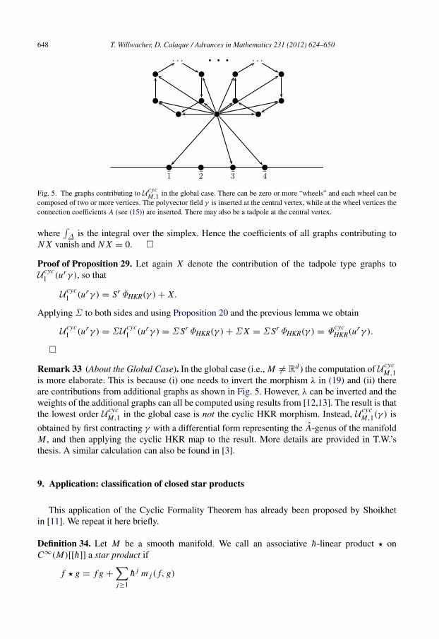
Fig. 5. The graphs contributing to U cycM,1 in the global case. There can be zero or more “wheels” and each wheel can be

composed of two or more vertices. The polyvector field γ is inserted at the central vertex, while at the wheel vertices theconnection coefficients A (see (15)) are inserted. There may also be a tadpole at the central vertex.

where∆ is the integral over the simplex. Hence the coefficients of all graphs contributing to

N X vanish and N X = 0.

Proof of Proposition 29. Let again X denote the contribution of the tadpole type graphs toU cyc

1 (urγ ), so that

U cyc1 (urγ ) = SrΦHKR(γ )+ X.

Applying Σ to both sides and using Proposition 20 and the previous lemma we obtain

U cyc1 (urγ ) = Σ U cyc

1 (urγ ) = Σ SrΦHKR(γ )+ Σ X = Σ SrΦHKR(γ ) = ΦcycHKR(u

rγ ).

Remark 33 (About the Global Case). In the global case (i.e., M = Rd ) the computation of U cycM,1

is more elaborate. This is because (i) one needs to invert the morphism λ in (19) and (ii) thereare contributions from additional graphs as shown in Fig. 5. However, λ can be inverted and theweights of the additional graphs can all be computed using results from [12,13]. The result is thatthe lowest order U cyc

M,1 in the global case is not the cyclic HKR morphism. Instead, U cycM,1(γ ) is

obtained by first contracting γ with a differential form representing the A-genus of the manifoldM , and then applying the cyclic HKR map to the result. More details are provided in T.W.’sthesis. A similar calculation can also be found in [3].

9. Application: classification of closed star products

This application of the Cyclic Formality Theorem has already been proposed by Shoikhetin [11]. We repeat it here briefly.

Definition 34. Let M be a smooth manifold. We call an associative h-linear product ⋆ onC∞(M)[[h]] a star product if

f ⋆ g = f g +j≥1

h j m j ( f, g)


for bidifferential operators m j and all f, g ∈ C∞(M). Two star products ⋆, ⋆′ are gaugeequivalent if there is a formal series of differential operators

D = 1+j≥1

h j D j

such that f ⋆g = D−1(D( f ) ⋆′ D(g)) for all f, g ∈ C∞(M). Let now M be oriented with volumeform ω. The star product ⋆ is closed if for any three compactly supported f, g, h ∈ C∞c (M)

Mf (g ⋆ h)ω =

M

g(h ⋆ f )ω.

Two closed star products ⋆, ⋆′ are called gauge equivalent if there is a D as above such thatf ⋆ g = D−1(D( f ) ⋆′ D(g)) and

Mf gω =

M

D( f )D(g)ω

for all f, g ∈ C∞c (M).

Remark 35. Note that we do not require the constant function 1 to be a unit to the deformedalgebra. However, it is easy to show that a unit 1 = 1 + O(h) still exists. Furthermore, thefunctional

tr : f →

Mf 1ω

defines a trace on the compactly supported subalgebra, i.e., tr( f ⋆ g) = tr(g ⋆ f ) for f, g (or atleast one of them) compactly supported.

Definition 36. A formal series of degree 1 elements of T •+1poly [u]

π =j≥1

h j (π j + u f j )

is called formal unimodular Poisson structure if u divπ + 12 [π, π]S = 0. Two such π , π ′ are

gauge equivalent if there is a formal series of vector fields

ξ =j≥1

h j ξ j

such that

π ′ = eadξπ + u1− eadξ

adξdiv ξ

where adξ (·) := [ξ, ·]S .

The above notions of gauge equivalence define equivalence relations on the sets of closedstar products and formal unimodular Poisson structures. There is a map Φ between the two sets,mapping a formal unimodular Poisson structure π to the (closed) star product ⋆ such that

f ⋆ g = f g +j≥1

1j !

U cycM, j (π ⊙ · · · ⊙ π)( f, g).


Theorem 37. The map Φ is a bijection between the set of gauge equivalence classes of formalunimodular Poisson structures and the set of gauge equivalence classes of closed star products.

Proof. Kontsevich has shown in [9] that an L∞-quasi-isomorphism between DGLAs g → g′

induces in the above manner a bijection between the gauge equivalence classes of solutions tothe Maurer–Cartan equations in the pro-nilpotent Lie algebras hg[[h]] and hg′[[h]]. Applyingthis to g = Tpoly(M)[u] and g′ = (Dpoly(M))σ yields the result.

Acknowledgments

This paper is a part of T. W.’s Ph.D. thesis, written at ETH Zurich. T. W. is very grateful tohis advisor Giovanni Felder for his support and teaching, and for reading the manuscript andproviding valuable comments.

T. W. was partially supported by the Swiss National Science Foundation (grant 200020-105450). The research of D. C. was fully supported by the European Union thanks to a MarieCurie Intra-European Fellowship (contract number MEIF-CT-2007-042212).

References

[1] D. Arnal, D. Manchon, M. Masmoudi, Choix des signes pour la formalite de M. Kontsevich, Pacific J. Math. 203(1) (2002) 23–66. arXiv:math/0003003.

[2] A.S. Cattaneo, G. Felder, Effective batalin-vilkovisky theories, equivariant configuration spaces and cyclic chains,in: A.S. Cattaneo, A. Giaquinto, P. Xu (Eds.), Higher Structures in Geometry and Physics: in honor of MurrayGerstenhaber and Jim Stasheff, in: Progress in Mathematics, vol. 287, Birkhauser, Boston, 2011, pp. 111–137.

[3] A.S. Cattaneo, G. Felder, T. Willwacher, The character map in deformation quantization, 2011. arXiv:0906.3122.[4] V. Dolgushev, Covariant and equivariant formality theorems, Adv. Math. 191 (2005) 147. arXiv:math/0307212.[5] V. Dolgushev, A proof of Tsygan’s formality conjecture for an arbitrary smooth manifold, Ph.D. Thesis, MIT, 2005.

arXiv:math/0504420.[6] V. Dolgushev, A formality theorem for Hochschild chains, Adv. Math. 200 (1) (2006) 51–101.[7] V. Dolgushev, D. Tamarkin, B. Tsygan, Formality theorems for Hochschild complexes and their applications, Lett.

Math. Phys. 90 (1) (2009) 103–136.[8] G. Felder, B. Shoikhet, Deformation quantization with traces, Lett. Math. Phys. 53 (1) (2000) 75–86.

arXiv:math/0002057.[9] M. Kontsevich, Deformation quantization of Poisson manifolds, Lett. Math. Phys. 66 (3) (2003) 157–216.

[10] J.-L. Loday, Cyclic homology, in: Grundlehren der Mathematischen Wissenschaften (Fundamental Principles ofMathematical Sciences), vol. 301, Springer-Verlag, Berlin, 1992.

[11] B. Shoikhet, On the cyclic formality conjecture, 1999. arxiv:math/9903183.[12] M. Van den Bergh, The Kontsevich weight of a wheel with spokes pointing outward, Algebr. Represent. Theory 12

(2009) 443–479. http://dx.doi.org/10.1007/s10468-009-9161-6.[13] T. Willwacher, A counterexample to the quantizability of modules, Lett. Math. Phys. 81 (3) (2007) 265–280.

arXiv:0706.0970.

http://arxiv.org/math/0003003

http://arxiv.org/0906.3122





http://dx.doi.org/doi:10.1007/s10468-009-9161-6

http://arxiv.org/0706.0970

Formality of cyclic cochains - core.ac.uk · Section4recalls the definition ... For the special...

Documents

Transcript of Formality of cyclic cochains - core.ac.uk · Section4recalls the definition ... For the special...