Lecture Notes For

Formal Languages and Automata

Gordon J. PaceDecember 1997

Department of Computer Science & A.I.Faculty of ScienceUniversity of Malta

Contents

1 Introduction and Motivation 51.1 Introduction . . . . . . . . . . . . . . . . . . . . . . . . . . . . 51.2 Grammar Representation . . . . . . . . . . . . . . . . . . . . . 71.3 Discussion . . . . . . . . . . . . . . . . . . . . . . . . . . . . . 101.4 Exercises . . . . . . . . . . . . . . . . . . . . . . . . . . . . . . 11

2 Languages and Grammars 132.1 Introduction . . . . . . . . . . . . . . . . . . . . . . . . . . . . 132.2 Alphabets and Strings . . . . . . . . . . . . . . . . . . . . . . 132.3 Languages . . . . . . . . . . . . . . . . . . . . . . . . . . . . . 15

2.3.1 Exercises . . . . . . . . . . . . . . . . . . . . . . . . . . 162.4 Grammars . . . . . . . . . . . . . . . . . . . . . . . . . . . . . 17

2.4.1 Exercises . . . . . . . . . . . . . . . . . . . . . . . . . . 212.5 Properties and Proofs . . . . . . . . . . . . . . . . . . . . . . . 21

2.5.1 A Simple Example . . . . . . . . . . . . . . . . . . . . 222.5.2 A More Complex Example . . . . . . . . . . . . . . . . 232.5.3 Exercises . . . . . . . . . . . . . . . . . . . . . . . . . . 26

2.6 Summary . . . . . . . . . . . . . . . . . . . . . . . . . . . . . 27

3 Classes of Languages 283.1 Motivation . . . . . . . . . . . . . . . . . . . . . . . . . . . . . 283.2 Context Free Languages . . . . . . . . . . . . . . . . . . . . . 28

3.2.1 Definitions . . . . . . . . . . . . . . . . . . . . . . . . . 283.2.2 Context free languages and the empty string . . . . . . 293.2.3 Derivation Order and Ambiguity . . . . . . . . . . . . 353.2.4 Exercises . . . . . . . . . . . . . . . . . . . . . . . . . . 38

3.3 Regular Languages . . . . . . . . . . . . . . . . . . . . . . . . 403.3.1 Definitions . . . . . . . . . . . . . . . . . . . . . . . . . 41

2

3.3.2 Properties of Regular Grammars . . . . . . . . . . . . 413.3.3 Exercises . . . . . . . . . . . . . . . . . . . . . . . . . . 443.3.4 Properties of Regular Languages . . . . . . . . . . . . . 45

3.4 Conclusions . . . . . . . . . . . . . . . . . . . . . . . . . . . . 52

4 Finite State Automata 534.1 An Informal Introduction . . . . . . . . . . . . . . . . . . . . . 53

4.1.1 A Different Representation . . . . . . . . . . . . . . . . 544.1.2 Automata and Languages . . . . . . . . . . . . . . . . 554.1.3 Automata and Regular Languages . . . . . . . . . . . . 56

4.2 Deterministic Finite State Automata . . . . . . . . . . . . . . 594.2.1 Implementing a DFSA . . . . . . . . . . . . . . . . . . 634.2.2 Exercises . . . . . . . . . . . . . . . . . . . . . . . . . . 64

4.3 Non-deterministic Finite State Automata . . . . . . . . . . . . 644.4 Formal Comparison of Language Classes . . . . . . . . . . . . 67

4.4.1 Exercises . . . . . . . . . . . . . . . . . . . . . . . . . . 76

5 Regular Expressions 785.1 Definition of Regular Expressions . . . . . . . . . . . . . . . . 785.2 Regular Grammars and Regular Expressions . . . . . . . . . . 805.3 Exercises . . . . . . . . . . . . . . . . . . . . . . . . . . . . . . 845.4 Conclusions . . . . . . . . . . . . . . . . . . . . . . . . . . . . 85

6 Pushdown Automata 876.1 Stacks . . . . . . . . . . . . . . . . . . . . . . . . . . . . . . . 876.2 An Informal Introduction . . . . . . . . . . . . . . . . . . . . . 886.3 Non-deterministic Pushdown Automata . . . . . . . . . . . . . 896.4 Pushdown Automata and Languages . . . . . . . . . . . . . . 93

6.4.1 From CFLs to NPDA . . . . . . . . . . . . . . . . . . . 936.4.2 From NPDA to CFGs . . . . . . . . . . . . . . . . . . 96

6.5 Exercises . . . . . . . . . . . . . . . . . . . . . . . . . . . . . . 101

7 Minimization and Normal Forms 1037.1 Motivation . . . . . . . . . . . . . . . . . . . . . . . . . . . . . 1037.2 Regular Languages . . . . . . . . . . . . . . . . . . . . . . . . 105

7.2.1 Overview of the Solution . . . . . . . . . . . . . . . . . 1057.2.2 Formal Analysis . . . . . . . . . . . . . . . . . . . . . . 1067.2.3 Constructing a Minimal DFSA . . . . . . . . . . . . . 111

3

7.2.4 Exercises . . . . . . . . . . . . . . . . . . . . . . . . . . 1157.3 Context Free Grammars . . . . . . . . . . . . . . . . . . . . . 116

7.3.1 Chomsky Normal Form . . . . . . . . . . . . . . . . . . 1167.3.2 Greibach Normal Form . . . . . . . . . . . . . . . . . . 1207.3.3 Exercises . . . . . . . . . . . . . . . . . . . . . . . . . . 1257.3.4 Conclusions . . . . . . . . . . . . . . . . . . . . . . . . 126

4

Chapter 1

Introduction and Motivation

1.1 Introduction

What is a language? Whether we restrict our discussion to natural languagessuch as English or Maltese, or whether we also discuss artificial languagessuch as computer languages and mathematics, the answer to the questioncan be split into two parts:

Syntax: An English sentence of the form:

〈noun-phrase〉 〈verb〉 〈noun-phrase〉

(such as The cat eats the cheese) has a correct structure (assumingthat the verb is correctly conjugated). On the other hand, a sentenceof the form 〈adjective〉 〈verb〉 (such as red eat) does not make sensestructurally. A sentence is said to be syntactically correct if it is builtfrom a number of components which make structural sense.

Semantics: Syntax says nothing about the meaning of a sentence. In facta number of syntactically correct sentences make no sense at all. Theclassic example is a sentence from Chomsky:

Colourless green ideas sleep furiously

Thus, at a deeper level, sentences can be analyzed semantically to checkwhether they make any sense at all.

5

In mathematics, for example, all expressions of the form x/y are usuallyconsidered to be syntactically correct, even though 10/0 usually correspondsto no meaningful semantic interpretation.

In spoken natural language, we regularly use syntactically incorrect sen-tences, even though the listener usually manages to ‘fix’ the syntax andunderstand the underlying semantics as meant by the speaker. This is par-ticularly evident in baby-talk. At least babies can be excused, however poetshave managed to make an art out of it!

There was a poet from ZejtunWhose poems were strange, out-of-tune,Correct metric they had,The rhyme wasn’t that bad,But his grammar sometimes like baboon.

For a more accomplished poet and author, may I suggest you read one of thepoems in Lewis Carroll’s ‘Alice Through the Looking Glass’, part of whichgoes:

’Twas brillig, and the slithy tovesDid gyre and gimble in the wabe:All mimsy were the borogoves,And the mome raths outgrabe.

In computer languages, a compiler generates errors of a syntactic nature.Semantic errors appear at run-time when the computer is interpreting thecompiled code.

In this course we will be dealing with the syntactic correctness of languages.Semantics shall be dealt with in a different course.

However, splitting the problem into two, and choosing only one thread tofollow, has not made the solution much easier. Let us start by listing anumber of properties which seem evident:

• a number of words (or symbols or whatever) are used as the basicbuilding blocks of a language. Thus in mathematics, we may havenumbers whereas in English we would have English words.

• certain sequences of the basic symbols are allowed (are valid sentencesin the language) whereas others are not.

6

This characterizes completely what a language is: a set of sequences of sym-bols. So for example, English would be the set:

{The cat ate the mouse, I eat, . . .}Note that this set is infinite (The house next to mine is red, The house next tothe one next to mine is red, The house next to the one next to the one next tomine is red, etc are all syntactically valid English sentences), however, it doesnot include certain sequences of words (such as But his grammar sometimeslike baboon).

Enlisting an infinite set is not the most pleasant of jobs. Furthermore, thisalso creates a paradox. Our brains are of finite size, so how can they containan infinite language? The solution is actually rather simple: the languageswe are mainly interested in can be generated from a finite number of rules.Thus, we need not remember whether I eat is syntactically valid, but wementally apply a number of rules to deduce its validity.

Languages with which we are concerned are thus a finite set of basic sym-bols, together with a finite set of rules. These rules, the grammar of thelanguage, allow us to generate sequences of the basic symbols (usually calledthe alphabet). Sequences we can generate are syntactically correct sentencesof the languages, whereas ones we cannot are syntactically incorrect.

Valid Pascal variable names can be generated from the letters and numbers(‘A’ to ‘Z’, ‘a’ to ‘z’ and ‘0’ to ‘9’) and the underscore symbol (‘ ’). A validvariable name starts with a letter and may then follow with any number ofsymbols from the alphabet. Thus, I_am_not_a_variable is a valid variablename, whereas 25_lettered_variable_name is not.

The next problem to deal with is the representation of language’s gram-mar. Various solutions have been proposed and tried out. Some are simplyincapable of describing certain desirable grammars. Of the more generalrepresentations some are better suited than others to be used in certain cir-cumstances.

1.2 Grammar Representation

Computer language manuals usually use the BNF (Backus-Naur Form) no-tation to describe the syntax of the language. The grammar of the variablenames as described earlier can be given as:

7

〈letter〉 ::= a | b | . . . z | A | B | . . . Z〈number〉 ::= 0 | 1 | . . . 9〈underscore〉 ::= _〈misc〉 ::= 〈letter〉 | 〈number〉 | 〈underscore〉〈end-of-var〉 ::= 〈misc〉 | 〈misc〉〈end-of-var〉〈variable〉 ::= 〈letter〉 | 〈letter〉〈end-of-var〉

The rules are read as definitions. The ‘::=’ symbol is the definition sym-bol, the | symbol is read as ‘or’ and adjacent symbols denote concatenation.Thus, for example, the last definition states that a string is a valid 〈variable〉if it is either a valid 〈letter〉 or a valid 〈letter〉 concatenated with a valid〈end-of-var〉. The names in angle brackets (such as 〈letter〉) do not appearin valid strings but may be used in the derivation of such strings. For this rea-son, these are called non-terminal symbols (as opposed to terminal symbolssuch as a and 4).

Another representation frequently used in computing especially when de-scribing the options available when executing a program looks like:

cp [-r] [-i] 〈file-name〉 〈file-name〉|〈dir-name〉

This partially describes the syntax of the copy command in UNIX. It saysthat a copy command starts with the string cp. It may then be followedby -r and similarly -i (strings enclosed in square brackets are optional). Afilename is then given followed by a file or directory name (| is choice).

Sometimes, this representation is extended to be able to represent more usefullanguages. A string followed by an asterisk is used to denote 0 or morerepetitions of that string, and a string followed by a plus sign used to denote1 or more repetitions. Bracketing may also be used to make precedence clear.Thus, valid variable names may be expressed by:

a|b . . . Z (a|b . . . Z|_|0|1| . . . 9)*

Needless to say, it quickly becomes very complicated to read expressionswritten in this format.

Another standard way of expressing programming language portions is byusing syntax diagrams (sometimes called ‘railroad track’ diagrams). Belowis a diagram taken from a book on standard C to define a postfix operator.

8

--

expression

expression

++

][

,

( )

name

name

.

->

Even though you probably do not have the slightest clue as to what a postfixoperator is, you can deduce from the diagram that it is either simply ++,or −−, or an expression within square brackets, or a list of expressions inbrackets or a name preceded by a dot or by ->. The definition of expressionsand names would be similarly expressed. The main strength of such a systemis ease of comprehension of a given grammar.

Another graphical representation uses finite state automata. A finite stateautomaton has a number of different named states drawn as circles. Labeledarrows are also drawn starting from and ending in states (possibly the same).One of the states is marked as the starting state (where computation starts),whereas a number of states are marked as final states (where computationmay end). The initial state is marked by an incoming arrow and the finalstates are drawn using two concentric circles. Below is a simple example ofsuch an automaton:

a

b

b

TS

The automaton starts off from the initial state and, upon receiving an input,moves along an arrow originating from the current state whose label is thesame as the given input. If no such arrow is available, the machine may beseen to ‘break’. Accepted strings are ones for which, when given as inputto the machine, result in a computation starting from the initial state andending in a terminal state without breaking the machine. Thus, in our ex-ample above b is accepted, as is ab and aabb. If we denote n repetitions of astring s by sn, we notice that the set of strings accepted by the automaton

9

is effectively:

{anbm | n ≥ 0 ∧m ≥ 1}

1.3 Discussion

These different notations give rise to a number of interesting issues which wewill discuss in the course of the coming lectures. Some of these issues are:

• How can we formalize these language definitions? In other words, wewill interpret these definitions mathematically in order to allow us toreason formally about them.

• Are some of these formalisms more expressive than others? Are therelanguages expressible in one but not another of these formalisms?

• Clearly, some of the definitions are simpler to implement as a computerprogram than others. Can we define a translation of a grammar fromone formalism to another, thus enabling us to implement grammarsexpressed in a difficult-to-implement notation by first translating theminto an alternative formalism?

• Clearly, even within the same formalism, certain languages can be ex-pressed in a variety of ways. Can we define a simplifying procedurewhich simplifies a grammar (possibly as an aid to implementation?)

• Again, given that some languages can be expressed in different waysin the same formalism, is there some routine way by which we cancompare two grammars and deduce their (in)equality?

On a more practical level, at the end of the course you should have a betterinsight into compiler writing. At least, you will be familiar with the syntaxchecking part of a compiler. You should also understand the inner workingsof LEX and YACC (standard compiler writing tools).

10

1.4 Exercises

1. What strings of type 〈S 〉 does the following BNF specification accept?

〈A〉 ::= a〈B〉 | a〈B〉 ::= b〈A〉 | b〈S 〉 ::= 〈A〉 | 〈B〉

2. What strings are accepted by the following finite state automaton?

1

00

1

+

- 1

00

1

’’N N N N1 1

3. A palindrome is a string which reads front-to-back the same as back-to-front. For example anna is a palindrome, as is madam. Write aBNF notation which accepts exactly all those palindromes over thecharacters a and b.

4. The correct (restricted) syntax for write in Pascal is as follows:

The instruction write is always followed by a parameter-list enclosedwithin brackets. A parameter-list is a comma-separated list of param-eters, where each parameter is either a string in quotes or a variablename.

(a) Write a BNF specification of the syntax

(b) Draw a syntax diagram

(c) Draw a finite state automaton which accept correct write state-ments (and nothing else)

5. Consider the following BNF specification portion:

〈exp〉 ::= 〈term〉 | 〈exp〉×〈exp〉 | 〈exp〉÷〈exp〉〈term〉 ::= 〈num〉 | . . .

An expression such as 2×3×4 can be accepted in different ways. Thisbecomes clear if we draw a tree to show how the expression has beenparsed. The two different trees for 2× 3× 4 are given below:

11

num num

num

num

x

x

2

3 4 2 3

4

x

x

term

exp

exp

exp

expexp

termtermnum

exp

term

num

term

term

exp exp

exp

exp

Clearly, different acceptance routes may have different meanings. Forexample (1 ÷ 2) ÷ 2 = 0.25 6= 1 = 1 ÷ (2 ÷ 2). Even though we arecurrently oblivious to issues regarding the semantics of a language, weidentify grammars in which there are sentences which can be acceptedin alternative ways. These are called ambiguous grammars.

In natural language, these ambiguities give rise to amusing misinter-pretations.

Today we will discuss sex with Margaret Thatcher

In computer languages, however, the results may not be as amusing.Show that the following BNF grammar is ambiguous by giving an ex-ample with the relevant parse trees:

〈program〉 ::= if 〈bool〉 then 〈program〉| if 〈bool〉 then 〈program〉 else 〈program〉

|...

12

Chapter 2

Languages and Grammars

2.1 Introduction

Recall that a language is a (possibly infinite) set of strings. A grammar toconstruct a language can be defined in terms of two pieces of information:

• A finite set of symbols which are used as building blocks in the con-struction of valid strings, and

• A finite set of rules which can be used to deduce strings. Strings ofsymbols which can be derived from the rules are considered to be stringsin the language being defined.

The aim of this chapter is to formalize the notions of a language and agrammar. By defining these concepts mathematically we then have the toolsto prove properties pertaining to these languages.

2.2 Alphabets and Strings

Definition: An alphabet is a finite set of symbols. We normally use variableΣ for an alphabet. Individual symbols in the alphabet will normally berepresented by variables a and b.

Note that with each definition, I will be including what I will normally useas a variable for the defined term. Consistent use of these variable namesshould make proofs easier to read.

13

Definition: A string over an alphabet Σ is simply a finite list of symbolsfrom Σ. Variables normally used are s, t, x and y.

The set of all strings over an alphabet Σ is usually written as Σ∗.

To make the expression of strings easier, we write their components withoutseparating commas or surrounding brackets, Thus, for example, [h, e, l, l, o]is usually written as hello.

What about the empty list? Since the empty string simply disappears whenusing this notation, we use symbol ε to represent it.

Definition: Juxtaposition of two strings is the concatenation of the twostrings. Thus:

stdef= s ++ t

This notation simplifies considerably the presentation of strings: Concate-nating hello with world is written as helloworld, which is precisely the resultof the concatenation!

Definition: A string s raised to a numeric power n (sn) is simply the cate-nation of n copies of s. This can be defined by:

s0 def= ε

sn+1 def= ssn

Definition: The length of a string s, written as |s|, is defined by:

|ε| def= 0

|ax| def= 1 + |x|

Note that a ∈ Σ and x ∈ Σ∗.

Definition: String s is said to be a prefix of string t, if there is some stringw such that t = sw.

Similarly, string s is said to be a postfix of string t, if there is some string wsuch that t = ws.

14

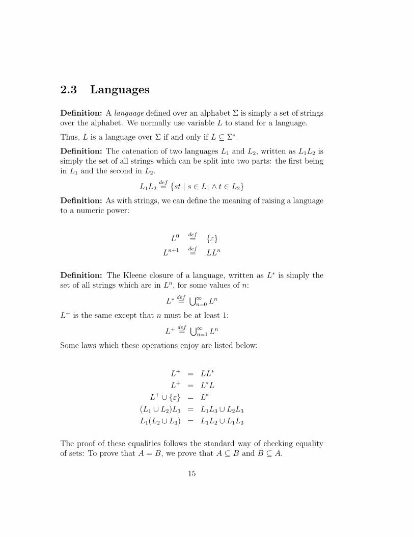
2.3 Languages

Definition: A language defined over an alphabet Σ is simply a set of stringsover the alphabet. We normally use variable L to stand for a language.

Thus, L is a language over Σ if and only if L ⊆ Σ∗.

Definition: The catenation of two languages L1 and L2, written as L1L2 issimply the set of all strings which can be split into two parts: the first beingin L1 and the second in L2.

L1L2def= {st | s ∈ L1 ∧ t ∈ L2}

Definition: As with strings, we can define the meaning of raising a languageto a numeric power:

L0 def= {ε}

Ln+1 def= LLn

Definition: The Kleene closure of a language, written as L∗ is simply theset of all strings which are in Ln, for some values of n:

L∗ def=

⋃∞n=0 Ln

L+ is the same except that n must be at least 1:

L+ def=

⋃∞n=1 Ln

Some laws which these operations enjoy are listed below:

L+ = LL∗

L+ = L∗L

L+ ∪ {ε} = L∗

(L1 ∪ L2)L3 = L1L3 ∪ L2L3

L1(L2 ∪ L3) = L1L2 ∪ L1L3

The proof of these equalities follows the standard way of checking equalityof sets: To prove that A = B, we prove that A ⊆ B and B ⊆ A.

15

Example: Proof of L+ = LL∗

x ∈ LL∗

⇔ definition of L∗

x ∈ L∞⋃

n=0

Ln

⇔ definition of concatenation

x = x1x2 ∧ x1 ∈ L ∧ x2 ∈∞⋃

n=0

Ln

⇔ definition of union

x = x1x2 ∧ x1 ∈ L ∧ ∃m ≥ 0 · x2 ∈ Lm

⇔ predicate calculus

∃m ≥ 0 · x = x1x2 ∧ x1 ∈ L ∧ x2 ∈ Lm

⇔ definition of concatenation

∃m ≥ 0 · x ∈ LLm

⇔ definition of Lm+1

∃m ≥ 0 · x ∈ Lm+1

⇔ ∃m ≥ 1 · x ∈ Lm

⇔ definition of union

x ∈∞⋃

n=1

Ln

⇔ definition of L+

x ∈ L+

2.3.1 Exercises

1. What strings do the following languages include:

(a) {a}{aa}∗

(b) {aa, bb}∗ ∩ ({a}∗ ∪ {b}∗)(c) {a, b, . . . z}{a, b, . . . z, 0, . . . 9}∗

2. What are L∅ and L{ε}?

16

3. Prove the four unproven laws of language operators.

4. Show that the laws about catenation and union do not apply to cate-nation and intersection by finding a counter-example which shows that(L1 ∩ L2)L3 6= L1L3 ∩ L2L3.

2.4 Grammars

A grammar is a finite mechanism which we will use to generate potentiallyinfinite languages.

The approach we will use is very similar to BNF. The strings we generate willbe built from symbols in a particular alphabet. These symbols are sometimesreferred to as terminal symbols. A number of non-terminal symbols will beused in the computation of a valid string. These appear in our BNF grammarswithin angle brackets. Thus, for example, in the following BNF grammar,the alphabet is {a, b}1 and the non-terminal symbols are {〈W 〉, 〈A〉, 〈B〉}.〈W 〉 ::= 〈A〉 | 〈B〉〈A〉 ::= a〈A〉 | ε〈B〉 ::= b〈B〉 | ε

The BNF grammar is defining a number of transition rules from a non-terminal symbol to strings of terminal and non-terminal symbols. We choosea more general approach, where transition rules transform a non-empty stringinto another (potentially empty) string. These will be written in the form:from → to. Thus, the above BNF grammar would be represented by thefollowing set of transitions:

{W → A|B, A → aA|ε, B → bB|ε}Note that any rule of the form α → β|γ can be transformed into two rules ofthe form α → β and α → γ.

Only one thing remains. If we were to be given the BNF grammar justpresented, we would be unsure as to whether we are to accept strings whichcan be derived from 〈A〉 or from 〈B〉 or from 〈W 〉. It is thus necessary tospecify which non-terminal symbols derivations are to start from.

Definition: A phrase structure grammar is a 4-tuple 〈Σ, N, S, P 〉 where:

1Actually any set which includes both a and b but not any non-terminal symbols

17

Σ is the alphabet over which the grammar generates strings.N is a set of non-terminal symbols.S is one particular non-terminal symbol.P is a relation of type (Σ ∪N)+ × (Σ ∪N)∗.

It is assumed that Σ ∩N = ∅.Variables for non-terminals will be represented by uppercase letters and amixture of terminal and non-terminal symbols will usually be represented bygreek letters. G is usually used as a variable ranging over grammars.

The BNF grammar already given can thus be formalized to the phrase struc-ture grammar G = 〈Σ, N, S, P 〉, where:

Σ = {a, b}N = {W, A, B}S = W

P = { W → A,W → B,A → aA,A → ε,B → bB,B → ε }

We still have to formalize what we mean by a particular string being gener-ated by a certain grammar.

Definition: A string β is said to derive immediately from a string α ingrammar G, written α ⇒G β, if we can apply a production rule of G on asubstring of α obtaining β. Formally:

α ⇒G βdef= ∃α1, α2, α3, γ ·

α = α1α2α3 ∧β = α1γα3 ∧α2 → γ ∈ P

Thus, for example, in the grammar we obtained from the BNF specification,we can prove that:

18

S ⇒G aA

S ⇒G bB

aaaA ⇒G aaa

aaaA ⇒G aaaaA

SAB ⇒G SB

But not that:

S ⇒G a

A ⇒G a

SAB ⇒G aAAB

B ⇒G B

In particular, even though A ⇒G aA ⇒G a, it is not the case that A ⇒G a.With this in mind, we define the following relational closures of ⇒G:

α0⇒G β

def= α = β

αn+1⇒ G β

def= ∃γ · α ⇒G γ ∧ γ

n⇒G β

α∗⇒G β

def= ∃n ≥ 0 · α n⇒G β

α+⇒G β

def= ∃n ≥ 1 · α n⇒G β

It can thus be proved that:

S∗⇒G a

A∗⇒G a

SAB∗⇒G aAAB

B∗⇒G B

although it is not the case that B+⇒G B.

19

Definition: A string α ∈ (N∪Σ)∗ is said to be in sentential form in grammarG if it can be derived from S, the start symbol of G. S(G) is the set of allsentential forms in G:

S(G)def= {α : (N ∪ Σ)∗ | S ∗⇒G α}

Definition: Strings in sentential form built solely from terminal symbols arecalled sentences.

These definitions indicate clearly what we mean by the language generatedby a grammar G. It is simply the set of all strings of terminal symbols whichcan be derived from the start symbol in any number of steps.

Definition: The language generated by grammar G, written as L(G) is theset of all sentences in G:

L(G)def= {x : Σ∗ | S +⇒G x}

Proposition: L(G) = S(G) ∩ Σ∗

For example, in the BNF example, we should now be able to prove that thelanguage described by the grammar is the set of all strings of the form an

and bn, where n ≥ 0.

L(G) = {an | n ≥ 0} ∪ {bn | n ≥ 0}

Now consider the alternative grammar G′ = 〈Σ′, N ′, S ′, P ′〉:

Σ′ = {a, b}N ′ = {W, A, B}S ′ = W

P ′ = { W → A,W → B,W → ε,A → a,A → Aa,aAa → a,B → bB,B → b }

20

With some thought, it should be obvious that L(G) = L(G′). This gives riseto a convenient way of comparing grammars — by comparing the languagesthey produce.

Definition: The grammars G1 and G2 are said to be equivalent if theyproduce the same language: L(G1) = L(G2).

2.4.1 Exercises

1. Show how aaa can be derived in G.

2. Show two alternative ways in which aaa can be derived in G′.

3. Give a grammar which produces only (and all) palindromes over thesymbols {a, b}.

4. Consider the alphabet Σ = {+, =, ·}. Repetitions of · are used to rep-resent numbers (·n corresponding to n). Define a grammar to produceall valid sums such as · ·+· = · · ·.

5. Define a grammar which accepts strings of the form anbncn (and noother strings).

2.5 Properties and Proofs

The main reason behind formalizing the concept of languages and grammarswithin a mathematical framework is to allow formal reasoning about theseentities.

A number of different techniques are used to prove different properties. How-ever, basically all proofs use induction in some way or another.

The following examples attempt to show different techniques as used in proofsof different properties or grammars. It is however, very important that otherexamples are tried out to experience the ‘discovery’ of a proof, which theseexamples cannot hope to convey.

21

2.5.1 A Simple Example

We start off with a simple grammar and prove what the language generatedby the grammar actually contains.

Consider the phrase structure grammar G = 〈Σ, N, S, P 〉, where:

Σ = {a}N = {B}S = B

P = {B → ε | aB}

Intuitively, this grammar includes all, and nothing but a sequences. How dowe prove this?

Theorem: L(G) = {an|n ≥ 0}

Proof: Notice that we are trying to prove the equality of two sets. In otherwords, we want to prove two statements:

1. L(G) ⊆ {an|n ≥ 0}, or that all sentences are of the form an,

2. {an|n ≥ 0} ⊆ L(G), or that all strings of the form an are generated bythe grammar.

Proof of (1): Looking at the grammar, and using intuition, it is obvious thatall sentential forms are of the form: anB or an.

This is formally proved by induction on the length of derivation. In otherwords, we prove that any sentential form derived in one step is of the desiredform, and that, if any sentential form derived in k steps takes the given form,so should any sentential form derivable in k + 1 steps. By induction we thenconclude that derivations of any length have the given structure.

Consider B1⇒G α. From the grammar, α is either ε = a0 or aB, both of

which have the desired structure.

Assume that all derivations of length k result in the desired format. Now

consider a k + 1 length relation: Bk+1⇒G β.

22

But this implies that Bk⇒G α

1⇒G β, where, by induction, α is either of theform anB or an. Clearly, we cannot derive any β from an, and if α =anBthen β =an+1B or β =an+1 both of which have the desired structure.

Hence, by induction, S(G) ⊆ {an, anB | n ≥ 0}. Thus:

x ∈ L(G)

⇔ x ∈ S(G) ∧ x ∈ Σ∗

⇒ x ∈ {an, anB | n ≥ 0} ∧ x ∈ a∗

⇔ x ∈ a∗

which completes the proof of (1).

Proof of (2): On the other hand, we can show that all strings of the formanB are derivable in zero or more steps from B.

The proof once again relies on induction, this time on n.

Base Case (n = 0): By definition of zero step derivations B0⇒G B. Hence

B∗⇒G B.

Inductive case: Assume that the property holds for n = k: B∗⇒G akB.

But akB1⇒G ak+1B, implying that B

∗⇒G ak+1B.

Hence, by induction, for all n, B∗⇒G anB. But anB ⇒G an. By definition

of derivations: B+⇒G an Thus, if x = an then x ∈ L(G):

{an|n ≥ 0} ⊆ L(G)�

Note: The proof for (1) can be given in a much shorter, neater way. Simplynote that L(G) ⊆ Σ∗. But Σ = {a}. Thus, L(G) ⊆ {a}∗ = {an | n ≥ 0}.The reason for giving the alternative long proof is to show how induction canbe used on the length of derivation.

2.5.2 A More Complex Example

As a more complex example, we will now treat a palindrome generatinggrammar. To reason formally, we need to define a new operator, the reversalof a string, written as sR. This is defined by:

23

εR def= ε

(ax)R def= xRa

The set of all palindromes over an alphabet Σ can now be elegantly writtenas: {wwR | w ∈ Σ∗} ∪ {wawR | a ∈ Σ∧w ∈ Σ∗}. We will abbreviate this setto PalΣ.

The grammar G′ = 〈Σ′, N ′, S ′, P ′〉, defined below, should (intuitively)generate exactly the set of palindromes over {a, b}:

Σ = {a, b}N = {B}S = B

P = { B → a,B → b,B → ε,B → aBa,B → bBb }

Theorem: The language generated by G′ includes all palindromes: PalΣ ⊆L(G′).

Proof: If we can prove that all strings of the form wBwR (w ∈ Σ∗) arederivable in one or more steps from S, then, using the production rule B → ε,we can generate any string from the first set in one or more productions:

B∗⇒G′ wBwR ⇒′

G wwR

Similarly, using the rules B → a and B → b, we can generate any string inthe second set.

Now, we must prove that all wBwR are in sentential form. The proof proceedsby induction on the length of string w.

Base case |w| = 0: By definition of∗⇒G′ , B

∗⇒G′ B = εBεR.

Inductive case: Assume that for any terminal string w of length k, B∗⇒G′

wBwR.

24

Given a string w′ of length k + 1, w′ = wa or w′ = wb, for some string w oflength k. Hence, by the inductive hypothesis: B

∗⇒G′ wBwR.

Consider the case for w′ = wa. Using the production rule B → aBa:

B∗⇒G′ wBwR ⇒′

G waBawR = w′Bw′R

Hence B∗⇒G′ w′Bw′R, completing the proof.

�

Theorem: Furthermore, the grammar generates only palindromes.

Proof: If we now prove that all sentential forms have the structure wBwR

or wwR or wcwR (where w ∈ Σ∗ and c ∈ Σ), recall that L(G) = S(G) ∩ Σ∗.Thus, it can then be proved that LG ⊆ {wwR | w ∈ Σ∗} ∪ {wcwR | c ∈Σ ∧ w ∈ Σ∗} = PalΣ.

To prove that all sentential forms are in one of the given structures, we useinduction on the length of the derivation.

Base case (length 1): If B1⇒G′ α, α takes the form of one of: ε, a, b, aBa,

bBb, all of which are in the desired form.

Inductive case: Assume that all derivations of length k result in an expressionof the desired form.

Now consider a derivation k+1 steps long. Clearly, we can split the derivationinto two parts, one k steps long, and one last step:

Bk⇒G′ α

1⇒G′ β

Using the inductive hypothesis, α must be in the form of wBwR or wwR orwcwR. The last two are impossible, since otherwise there would be no laststep to take (the production rules all transform a non-terminal which is notpresent in the last two cases). Thus, α = wBwR for some string of terminalsw.

From this α we get only a limited number of last steps, forcing β to be:

• wwR

• wawR

• wbwR

• waBawR = (wa)B(wa)R

25

• wbBbwR = (wb)B(wb)R

All of which are in the desired format. Thus, any derivation k + 1 steps longproduces a string in one of the given forms. This completes the induction,proving that that all sentential forms have the structure wBwR, wwR orwcwR, which completes the proof.

�

2.5.3 Exercises

1. Consider the following grammar:

G = 〈Σ, N, S, P 〉, where:

Σ = {a, b}N = {S, A, B}P = { S → AB,

A → ε | aA,B → b | bB }

Prove that L(G) = {anbm|n ≥ 0, m > 0}

2. Consider the following grammar:

G = 〈Σ, N, S, P 〉, where:

Σ = {a, b}N = {S, A, B}P = { S → aB | A,

A → bA | S,B → bS | b }

Prove that:

(a) Prove that any string in L(G) is at least two symbols long.

26

(b) For any string x ∈ L(G), x always ends with a b.

(c) The number of occurances of b in a sentence in the language gen-erated by G is not less than the number of occurances of a.

2.6 Summary

The following points should summarize the contents of this part of the course:

• A language is simply a set of finite strings over an alphabet.

• A grammar is a finite means of deriving a possibly infinite languagefrom a finite set of rules.

• Proofs about languages derived from a grammar usually use inductionover one of a number of variables, such as length of derivation, lengthof string, number of occurances of a symbol in the string, etc.

• The proofs are quite simple and routine once you realize how inductionis to be used. The bulk of the time taken to complete a proof is takenup sitting at a table, staring into space and waiting for inspiration. Donot get discouraged if you need to dwell on a problem for a long timeto find a solution. Practice should help you speed up inspiration.

27

Chapter 3

Classes of Languages

3.1 Motivation

The definition of a phrase structure grammar is very general in nature. Im-plementing a language checking program for a general grammar is not a triv-ial task and can be very inefficient. This part of the course identifies someclasses of languages which we will spend the rest of the course discussing andproving properties of.

3.2 Context Free Languages

3.2.1 Definitions

One natural way of limiting grammars is to allow only production rules whichderive a string (of terminals and non-terminals) from a single non-terminalsymbol. The basic idea is that in this class of languages, context information(the symbols surrounding a particular non-terminal symbol) does not matterand should not change how a string evolves. Furthermore, once a terminalsymbol is reached, it cannot evolve any further. From these restrictions,grammars falling in this class are called context free grammars. An obviousquestion arising from the definition of this class of languages is: does it in factreduce the set of languages produced by general grammars? Or conversely,can we construct a context free grammar for any language produced by aphrase structure grammar? The answer is negative. Certain languages, pro-duced by a phrase structure grammar cannot be generated by a context free

28

grammar. An example of such a language is {anbncn | n ≥ 0}. It is beyondthe scope of this introductory course to prove the impossibility of construct-ing a context free grammar which recognizes this language, however you cantry your hand at showing that there is a phrase structure grammar whichgenerates this language.

Definition: A phrase structure grammar G = 〈Σ, N, P, S〉 is said to bea context free grammar if all the productions in P are in the form: A → α,where A ∈ N and α ∈ (Σ ∪N)∗.

Definition: A language L is said to be a context free language if there is acontext free grammar G such that L(G) = L.

Note that the constraints placed on BNF grammars are precisely those placedon context free languages. This gives us an extra incentive to prove propertiesabout this class of languages, since the results we obtain will immediatelybe applicable to a large number of computer language grammars alreadydefined1.

3.2.2 Context free languages and the empty string

Productions of the form α → ε are called ε-productions. It seems like awaste of effort to produce strings which then disappear into thin air! Thisseems to present one way of limiting context free grammars — by disallowingε-productions. But are we limiting the set of languages produced?

Definition: A grammar is said to be ε-free if it has no ε-productions exceptpossibly for S → ε (where S is the start symbol), in which case S does notappear on the right hand side of any rule.

Note that some texts define ε-free to imply no ε-productions at all.

Consider a language which includes the empty string. Clearly, there mustbe some rule which results in the empty string (possibly S → ε). Thus,certain languages cannot, it seems, be produced by a grammar which has noε-productions. However, as the following results show, the loss is not that

1This is, up to a certain extent, putting the carriage before the horse. When the BNFnotation was designed, the basic properties of context free grammars already known. Still,people all around the world continue to define computer language grammars in terms ofthe BNF notation. Implementing parsers for such grammars is made considerably easierby knowing some basic properties of context free languages.

29

great. For any context free language, there is an ε-free context free grammarwhich generates the language.

Lemma: For any context free grammar with no ε-productions G: G =〈Σ, N, P, S〉, we can construct a context free grammar G′ which is ε-freesuch that L(G′) = L(G) ∪ {ε}.Strategy: To prove the lemma we construct grammar G′. The new grammaris identical to G except that it starts off from a new start S ′ for which thereare two new production rules. S ′ → ε produces the desired empty string andS ′ → S guarantees that we also generate all the strings in G. G′ is obviouslyε free and it is intuitively obvious that it also generates L(G).

Proof: Define grammar G′ = 〈Σ, N ′, P ′, S ′〉 such that

N ′ = N ∪ {S ′} (where S ′ /∈ N)

P ′ = P ∪ {S ′ → ε, S ′ → S}

Clearly, G′ satisfies the constraints that it is an ε free context free grammarsince G itself is an ε free context free grammar. We thus need to prove thatL(G′) = L(G) ∪ {ε}.Part 1: L(G′) ⊆ L(G) ∪ {ε}.

Consider x ∈ L(G′). By definition, S ′ +⇒G′ x and x ∈ Σ∗.

By definition, S ′ +⇒G′ x if, either:

• S ′ 1⇒G′ x, which by case analysis of P ′ and the condition x ∈ Σ∗,implies that x = ε. Hence x ∈ L(G) ∪ {ε}.

• S ′ n+1⇒ G′ x, where n ≥ 1. This in turn implies that:

S ′ 1⇒G′ αn⇒G′ x

By case analysis of P ′, α = S. Furthermore, in the derivation Sn⇒G′ x,

S ′ does not appear (can be checked by induction on length of deriva-tion). Hence, it uses only production rules in P which guarantees thatS

n⇒G x (n ≥ 1).

Thus x ∈ L(G) ∪ {ε}.

30

Hence, x ∈ L(G′) ⇒ x ∈ L(G)∪{ε}, which is what is required to prove thatL(G′) ⊆ L(G) ∪ {ε}.Part 2: L(G) ∪ {ε} ⊆ L(G′)

This result follows similarly. If x ∈ L(G) ∪ {ε}, then either:

• x ∈ L(G) implying that S+⇒G x. But, since P ⊆ P ′, we can deduce

that:

S ′ ⇒′G S

+⇒G′ x

Implying that x ∈ L(G′).

• x ∈ {ε} implies that x = ε. From the definition of G′, S ′ ⇒′G ε, hence

ε ∈ L(G′).

Hence, in both cases, x ∈ L(G′), completing the proof.�

Example: Given the following grammar G, produce a new grammar G′

which satisfies L(G) ∪ {ε} = L(G′). G = 〈Σ, N, P, S〉 where:

Σ = {a, b}N = {S, A, B}P = { S → A | B | AB,

A → a | aA,B → b | bB }

Using the method used in the lemma just proved, we can write G′ = 〈Σ, N ∪{S ′}, P ′, S ′〉, where P ′ = P ∪ {S ′ → S | ε}, which is guaranteed to satisfythe desired property.

G′ = 〈Σ, N ′, P ′, S ′〉N ′ = {S ′, S, A, B}P ′ = { S ′ → ε | S,

S → A | B | AB,A → a | aA,B → b | bB }

31

Theorem: For any context free grammar G = 〈Σ, N, P, S〉, we canconstruct a context free grammar G′ with no ε-productions such that L(G′) =L(G) \ {ε}.

Strategy: Again we construct grammar G′ to prove the claim. The strategywe use is as follows:

• we copy all non-ε-productions from G to G′.

• for any non-terminal N which can become ε, we copy every rule inwhich N appears on the right hand side both with and without N .

Thus, for example, if A+⇒G ε, and there is a rule B → AaA in P , then we

add productions B → Aa, B → aA, B → AaA and B → a to P ′.

Clearly G′ satisfies the property of having no ε-productions, as required.However, the proof of equivalence (modulo ε) of the two languages is stillrequired.

Proof: Define G′ = 〈Σ, N, P ′, S〉, where P ′ is defined to be the union ofthe following sets of production rules:

• {A → α | α 6= ε, A → α ∈ P} — all non-ε-production rules in P .

• If Nε is defined to be the set of all non-terminal symbols from which εcan be derived (Nε = {A | A ∈ N, A

∗⇒G ε}), then we take the pro-duction rules in P and remove arbitrarily any number of non-terminalswhich are in Nε (making sure we do not end up with a ε-production).

By definition, G′ is ε-free. What is still left to prove is that L(G′) = L(G) \{ε}.

It suffices to prove that: For every x ∈ Σ∗ \ {ε}, S+⇒G x if and only if

S+⇒G′ x and that ε /∈ L(G′).

To prove the second statement we simply note that, to produce ε, the lastproduction must be an ε-production, of which G′ does not have any.

To prove the first, we start by showing that for every non-terminal A, x ∈Σ∗ \ {ε}, A

+⇒G x if and only if A+⇒G′ x. The desired result is simply a

special case (A = S) which would then complete the proof of the theorem.

32

Proof that A+⇒G x implies A

+⇒G′ x:

Proof by strong induction on the length of the derivation.

Base case: A1⇒G x. Thus, A → x ∈ P and also in P ′ (since it is not an

ε-production). Hence, A+⇒G′ x.

Assume it holds for any production taking up to k steps. We now need to

prove that Ak+1⇒G x implies A

+⇒G′ x.

But if Ak+1⇒G x then A

1⇒G X1 . . . Xnk⇒G x. x can also be split into n parts

(x = x1 . . . xn, some of which may be ε) such that Xi∗⇒G xi.

Now consider all non-empty xi: x = xλ1 . . . xλm . Since the productionsof these strings all take up to k steps, we can deduce from the inductive

hypothesis that: Xλi

+⇒G′ xλi. Since all the remaining non-terminals can

produce ε, we have a production rule (of the second type) in P ′: A →Xλ1 . . . Xλm .

Hence A ⇒′G Xλ1 . . . Xλm

+⇒G′ xλ1 . . . xλm = x, completing the induction.

Since all such productions take up to k steps, we can deduce from the induc-

tive principle that: Xi+⇒G′ xi for every non-empty xi.

Proof that A+⇒G′ x implies A

+⇒G x:�

Corollary: For any context free grammar G, we can construct an ε-freecontext free grammar G′ such that L(G′) = L(G).

Proof: The result follows immediately from the lemma and theorem justproved. From G, we can construct an context free grammar G′′ with noε-productions such that L(G′′) = L(G) \ {ε} (by theorem).

Now, if ε /∈ L(G), we have L(G′′) = L(G), hence G′ is defined to be G′′.Note that G′′ contains no ε-productions and is thus ε-free.

If ε ∈ L(G), using the lemma, we can produce a grammar G′ from G′′ suchthat L(G′) = L(G′′) ∪ {ε}, where G′ is ε-free. It can now be easily shownthat L(G′) = L(G).

�

Example: Construct an ε-free context free grammar and which generatesthe same language as G = 〈Σ, N, P, S〉:

33

Σ = {a, b}N = {S, A, B}P = { S → aA | bB | AabB,

A → ε | aA,B → ε | bS }

Using the method as described in the theorem, we construct a context freeG′ with no ε-productions such that L(G′) = L(G) \ {ε}. From the theorem,G′ = 〈Σ, N, P ′, S〉, where P ′ is the union of:

• The productions in P which are not ε-productions:

{S → aA | bB | AabB, A → aA, B → bS}

• Of the three non-terminals, A+⇒G ε and B

+⇒G ε, but ε cannot be de-rived from S (S immediately produces a terminal symbol which cannotdisappear since G is a context free grammar). We now rewrite all therules in P leaving out combinations of A and B:

{S → a | b | Aab | abB, A → a}

From the result of the theorem, L(G′) = L(G) \ {ε}. But ε /∈ L(G). Hence,L(G) \ {ε} = L(G). The result we need is G′:

G′ = 〈Σ, N, P ′, S〉Σ = {a, b}N = {S, A, B}P ′ = { S → a | b | aA | bB |

abB | Aab | AabB,A → a | aA,B → bS }

Example: Construct an ε-free context free grammar and which generatesthe same language as G = 〈Σ, N, P, S〉:

34

Σ = {a, b}N = {S, A, B}P = { S → A | B | ABa,

A → ε | aA,B → bS }

Using the theorem just proved, we will first define G′ which satisfies L(G′) =L(G) \ {ε}.

G′ def= 〈Σ, N, P ′, S〉 where P ′ is defined to be the union of:

• The non-ε-producing rules in P : {S → A | B | ABa, A → aA, B →bS}.

• The non-terminal symbols which can produce ε are A, S (S ⇒G A ⇒G

ε). Clearly B cannot produce ε. We now add all rules in P leavingout instances of A and S (which, in the process do not become ε-productions): {S → Ba, A → a, B → b}.

P ′ = { S → A | B | ABa | Ba,A → a | aA,B → b | bS }

However, ε ∈ L(G). We thus need to produce a context free grammar G′′

whose language is exactly that of G′ together with ε. Using the method fromthe lemma, we get G′′ = Σ, N ∪{S ′}, P ′′, S ′〉 where P ′′ = P ′∪{S → ε | S}.By the result of the theorem and lemma, G′′ is the grammar requested.

3.2.3 Derivation Order and Ambiguity

It has already been noted in the first set of exercises, that certain contextfree grammars are ambiguous, in the sense that for certain strings, more thanone derivation tree is possible.

The syntax tree is constructed as follows:

35

1. Draw the root of the tree with the initial non-terminal S written insideit.

2. Choose one leaf node with any non-terminal A written inside it.

3. Use any production rule (once) to derive a string α from A.

4. Add a child node to A for every symbol (terminal or non-terminal) inα, such that the children would read left-to-right α.

5. If there are any non-terminal leaves left, jump back to instruction 2.

Reading the terminal symbols from left to right gives the derived string x.The tree is called the syntax tree of x.

The sequence of production rules as used in the construction of the syntaxtree of x corresponds to a particular derivation of x from S. If the intermedi-ate trees during the construction read (as before, left to right) α1, α2, . . .αn,this would correspond to the derivation S ⇒G α1 ⇒G . . . ⇒G αn ⇒G x. Asthe forthcoming examples show, different syntax trees correspond to differentderivations, but different derivations may have a common syntax tree.

For example, consider the following grammar:

Gdef= 〈{a, b}, {S, A}, P, S〉

Pdef= {S → SA | AS | a, A → a | b}

Now consider the following two possible derivations of aab:

S ⇒G AS

⇒G ASA

⇒G ASb

⇒G aSb

⇒G aab

36

S ⇒G AS

⇒G ASA

⇒G aSA

⇒G aSb

⇒G aab

If we draw the derivation trees for both, we discover that they are, in factequivalent:

A

ba

S A

S

a

S

However, now consider another derivation of aab:

S ⇒G SA

⇒G SAA

⇒G aAA

⇒G aAb

⇒G aab

This has a different parse tree:

S

a

S A

a

b

S A

37

Hence G is an ambiguous grammar.

Thus, every syntax tree can be followed in a multitude of ways (as shown inthe previous example). A derivation is said to be a leftmost derivation if allderivation steps are done on the first (leftmost) non-terminal. Any tree thuscorresponds to exactly one leftmost derivation.

The leftmost derivation related to the first syntax tree of x is:

S ⇒G AS

⇒G aS

⇒G aSA

⇒G aaA

⇒G aab

while the leftmost derivation related to the second syntax tree of x is:

S ⇒G SA

⇒G SAA

⇒G aAA

⇒G aaA

⇒G aab

Since every syntax tree can be traversed left to right, and every leftmostderivation has a syntax tree, we can say that a grammar is ambiguous ifthere is a string x which has at least 2 distinct leftmost derivations.

3.2.4 Exercises

1. Given the context free grammar G:

G = 〈Σ, N, P, S〉

Σ = {a, b}

38

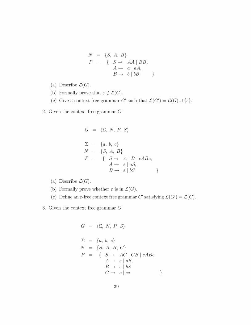
N = {S, A, B}P = { S → AA | BB,

A → a | aA,B → b | bB }

(a) Describe L(G).

(b) Formally prove that ε /∈ L(G).

(c) Give a context free grammar G′ such that L(G′) = L(G) ∪ {ε}.

2. Given the context free grammar G:

G = 〈Σ, N, P, S〉

Σ = {a, b, c}N = {S, A, B}P = { S → A | B | cABc,

A → ε | aS,B → ε | bS }

(a) Describe L(G).

(b) Formally prove whether ε is in L(G).

(c) Define an ε-free context free grammar G′ satisfying L(G′) = L(G).

3. Given the context free grammar G:

G = 〈Σ, N, P, S〉

Σ = {a, b, c}N = {S, A, B, C}P = { S → AC | CB | cABc,

A → ε | aS,B → ε | bSC → c | cc }

39

(a) Formally prove whether ε is in L(G).

(b) Define an ε-free context free grammar G′ satisfying L(G′) = L(G).

4. Give four distinct leftmost derivations of aaa in the grammar G definedbelow. Draw the syntax trees for these derivations.

Gdef= 〈{a, b}, {S, A}, P, S〉

Pdef= {S → SA | AS | a, A → a | b}

5. Show that the grammar below is ambiguous:

Gdef= 〈{a, b}, {S, A,B}, P, S〉

Pdef= { S → SA | AS | B,

A → a | b,B → b }

3.3 Regular Languages

Context free grammars are a convenient step down from general phrase struc-ture grammars. The popularity of the BNF notation indicates that thesegrammars are generally enough to describe the syntactic structure of generalprogramming languages. Furthermore, as we will see later, computationwise,these grammars can be conveniently parsed.

However, using the properties of context free grammars for certain languagesis like cracking a nut with a sledgehammer. If we were to define a simplersubset of grammars which is still general enough to include these smallerlanguages, we would have stronger results about this subset than we wouldhave about context free grammars, which might mean more efficient parsing.

Context free grammars limit what can appear on the left hand side of a parserule to a bare minimum (a single non-terminal symbol). If we are to simplifygrammars by placing further constraints on the production rules it has to be

40

on the right hand side of these rules. Regular grammars place exactly sucha constraint: Every rule must produce either a single terminal symbol, or asingle terminal symbol followed by a single non-terminal.

The constraints on the left hand side of production rules is kept the same,implying that every regular grammar is also a context free one. Again, wehave to ask the question: is every context free language also expressible bya regular grammar? In other words, is the class of context free languagesjust the same as the class of regular languages? The answer is once againnegative. {anbn | n ≥ 0} is a context free language (find the grammar whichgenerates it) but not a regular grammar.

3.3.1 Definitions

Definition: A phrase structure grammar G = 〈Σ, N, P, S〉 is said to be aregular grammar if all the productions in P are in on of the following forms:

• A → ε, where A ∈ N

• A → a, where A ∈ N and a ∈ Σ

• A → aB, where A, B ∈ N and a ∈ Σ

Note: This definition does not exclude multiple rules for a single non-terminal. Recall that, for example, A → a | aA is shorthand for the twoproduction rules A → a and A → aA. Both these rules are allowed inregular grammars, and thus so is A → a | aA.

Definition: A language L is said to be a regular language if there is a regulargrammar G such that L(G) = L.

3.3.2 Properties of Regular Grammars

Proposition: Every regular language is also a context free language.

Proof: If L is a regular language, there is a regular grammar G whichgenerates it. But every production rule in G has the form A → α whereA ∈ N . Thus, G is a context free grammar. Since G generates L, L is acontext free language.

41

�

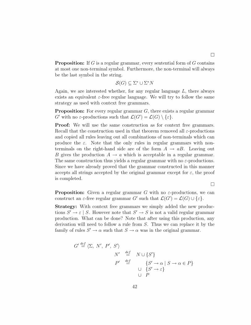
Proposition: If G is a regular grammar, every sentential form of G containsat most one non-terminal symbol. Furthermore, the non-terminal will alwaysbe the last symbol in the string.

S(G) ⊆ Σ∗ ∪ Σ∗N

Again, we are interested whether, for any regular language L, there alwaysexists an equivalent ε-free regular language. We will try to follow the samestrategy as used with context free grammars.

Proposition: For every regular grammar G, there exists a regular grammarG′ with no ε-productions such that L(G′) = L(G) \ {ε}.Proof: We will use the same construction as for context free grammars.Recall that the construction used in that theorem removed all ε-productionsand copied all rules leaving out all combinations of non-terminals which canproduce the ε. Note that the only rules in regular grammars with non-terminals on the right-hand side are of the form A → aB. Leaving outB gives the production A → a which is acceptable in a regular grammar.The same construction thus yields a regular grammar with no ε-productions.Since we have already proved that the grammar constructed in this manneraccepts all strings accepted by the original grammar except for ε, the proofis completed.

�

Proposition: Given a regular grammar G with no ε-productions, we canconstruct an ε-free regular grammar G′ such that L(G′) = L(G) ∪ {ε}.Strategy: With context free grammars we simply added the new produc-tions S ′ → ε | S. However note that S ′ → S is not a valid regular grammarproduction. What can be done? Note that after using this production, anyderivation will need to follow a rule from S. Thus we can replace it by thefamily of rules S ′ → α such that S → α was in the original grammar.

G′ def= 〈Σ, N ′, P ′, S ′〉

N ′ def= N ∪ {S ′}

P ′ def= {S ′ → α | S → α ∈ P}

∪ {S ′ → ε}∪ P

42

It is not difficult to prove the equivalence between the two grammars.�

Theorem: For every regular grammar G, there exists an equivalent ε-freeregular grammar G′.

Proof: We start by producing a regular grammar G′′ with no ε-productionssuch that L(G′′) = L(G) \ {ε} as done in the first proposition.

Clearly, if ε was not in the original language L(G) we now have an equivalentε-free regular grammar. If it was we use the construction in the secondproposition to add ε to the language.

�

Thus, in future discussions, we can freely discuss ε-free regular languageswithout having limited the scope of the discourse.

Example: Consider the regular grammar G:

Gdef= 〈Σ, N, P, S〉

Σdef= {a, b}

Ndef= {S, A, B}

Pdef= { S → aB | bA

A → b | bSB → a | aS }

Construct a regular grammar G′ such that L(G) ∪ {ε} = L(G′).

Using the method prescribed in the proposition, we construct a grammar G′

which starts off from a new state S ′, and can do everything G can do plusevolve from S ′ to the empty string (S ′ → ε) or to anything S can evolve to(S ′ → aB | bA):

G′ def= 〈Σ, N ′, P ′, S ′〉

N ′ def= {S ′, S, A, B}

P ′ def= { S ′ → aB | bA | ε

S → aB | bAA → b | bSB → a | aS }

43

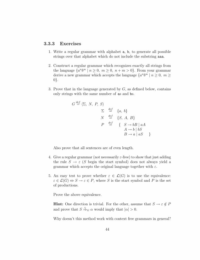
3.3.3 Exercises

1. Write a regular grammar with alphabet a, b, to generate all possiblestrings over that alphabet which do not include the substring aaa.

2. Construct a regular grammar which recognizes exactly all strings fromthe language {anbm | n ≥ 0, m ≥ 0, n + m > 0}. From your grammarderive a new grammar which accepts the language {anbm | n ≥ 0, m ≥0}.

3. Prove that in the language generated by G, as defined below, containsonly strings with the same number of as and bs.

Gdef= 〈Σ, N, P, S〉

Σdef= {a, b}

Ndef= {S, A, B}

Pdef= { S → bB | aA

A → b | bSB → a | aS }

Also prove that all sentences are of even length.

4. Give a regular grammar (not necessarily ε-free) to show that just addingthe rule S → ε (S begin the start symbol) does not always yield agrammar which accepts the original language together with ε.

5. An easy test to prove whether ε ∈ L(G) is to use the equivalence:ε ∈ L(G) ⇔ S → ε ∈ P , where S is the start symbol and P is the setof productions.

Prove the above equivalence.

Hint: One direction is trivial. For the other, assume that S → ε /∈ P

and prove that S+⇒G α would imply that |α| > 0.

Why doesn’t this method work with context free grammars in general?

44

3.3.4 Properties of Regular Languages

The language classes enjoy certain properties, some of which will be founduseful in proofs presented later in the course. This part of the course alsohelps to increase exposure to inductive proof techniques.

Both classes of languages defined so far are closed under union, catenationand Kleene closure. In other words, for example, given two regular languagesL1 and L2, their union L1∪L2, their catenation L1L2 and their Kleene closureL1

∗ are also regular languages. Similarly for two context free languages.

Here we will prove the result for regular languages since we will need it laterin the course. Closure of context free grammars will be treated in the secondyear course CSM 206 Language Hierarchies and Algorithmic Complexity.

The proofs are all by construction, which is another reason for their discus-sion. After understanding these proofs, for example, anyone can go out andmechanically construct a regular grammar accepting strings in either of twolanguages already specified using a regular grammar.

Theorem: If L is a regular grammar, so is L∗.

Strategy: The idea is to copy the production rules of a regular grammarwhich generates L and, for every rule in the form A → a (A ∈ N , a ∈ Σ)add also the rule A → aS, where S is the start symbol. Since S now appearson the right hand side of some rules, we leave out S → ε.

This way we have a grammar to generate L∗ \ {ε}. Since ε ∈ L∗, we thenadd ε by using the lemma in section 3.3.2.

Proof: Since L is a regular language, there must be a regular grammar Gsuch that L = L(G). We start off by defining a regular grammar G+ whichgenerates L∗ \ {ε}.Since ε ∈ L∗, we then use the lemma given in section 3.3.2 to construct aregular grammar G∗ from G+ such that:

L(G∗) = L(G+) ∪ {ε}= (L∗ \ {ε}) ∪ {ε}= L∗

which will complete the proof.

45

If G = 〈Σ, N, P, S〉, we define G+ as follows:

G+ def= 〈Σ, N, P+, S〉

P+ def=

P \ {S → ε}∪ {A → aS | A → a ∈ P, A ∈ N, a ∈ Σ}

We now need to show that L(G+) = L(G)∗ \ {ε}.

Proof of part 1: L(G+) ⊆ L(G)∗ \ {ε}

Assume that x ∈ L(G+). We prove by induction on the number of timesthat the new rules (P+ \ P ) were used in the derivation of x in G+.

Base case: If zero applications of the new rules appeared in S+⇒G+ x, S

+⇒G

x. Furthermore, there are no rules in G+ which allow x to be ε. Hence,L(G)∗ \ {ε}.

Inductive case: Assume that the result holds for derivations using the new

rules k times. Now consider x such that S+⇒G+ x, where the new rules have

been used k + 1 times.

If the last new rule used was A → aS, we can rewrite the derivation as:

S+⇒G+ sA ⇒+

G saS+⇒G+ saz = x

(Recall that all non-terminal sentential forms in a regular language must beof the form sA where s ∈ Σ∗ and A ∈ N)

Since no new rules have been used in the last part of the derivation: saS+⇒G

saz = x. Since all rules are applied exclusively to non-terminals: S+⇒G z

Furthermore, S+⇒G+ sA ⇒G sa is a valid derivation which uses only k

occurances of the new rules. Hence, by the inductive hypothesis: sa ∈L(G)∗ ⊆ {ε}.

Since x = saz x ∈ L(G)(L(G)∗ ⊆ {ε}) which implies that x ∈ L(G)∗ ⊆ {ε},completing the inductive proof.

Proof of part 2: L(G)∗ \ {ε} ⊆ L(G+)

Assume x ∈ L(G)∗ \ {ε}, then x ∈ L(G)n for some value of n ≥ 1. We provethat x ∈ L(G+) by induction on n.

46

Base case (n = 1): x ∈ L(G). Thus S+⇒G x. But since all the rules of G

are in G+, S+⇒G+ x. Hence x ∈ L(G+). Note that if S → ε appeared in P ,

S could not appear on the right hand side of rules, and hence if it was usedin the derivation of x, it must have been used immediately, implying thatx = ε.

Inductive case: Assume that all strings in L(G)k are in L(G+). Now considerx ∈ L(G)k+1. By definition, x = st where s ∈ L(G)k and t ∈ L(G).

By the induction hypothesis, s ∈ L(G+) which means that S+⇒G+ s. But if

the last rule applied was A → a: S∗⇒G+ wA ⇒+

G wa = s.

S∗⇒G+ wA ⇒+

G waS+⇒G+ wat = st

Hence x = st ∈ L(G+), completing the induction.�

Example: Consider grammar G which generates all sequences of a sand-wiched between an initial and final b:

G = 〈{a, b}, {S, A}, P.S〉P = {S → bA, A → aA | b}

To construct a new regular grammar G∗ such that L(G∗) = (L(G))∗, weapply the method used in Kleene’s theorem: we first copy all productionsfrom P to P ′ and, for every production of the form A → a in P (a is aterminal symbol), we also add the production A → aA to P ′, obtaininggrammar G′ in the process:

G′ = 〈{a, b}, {S, A}, P ′.S〉P = {S → bA, A → aA | b | bS}

Now we add ε to the language of G′ to obtain G∗:

G∗ = 〈{a, b}, {S∗, S, A}, P ′.S∗〉P = { S∗ → bA | ε

S → bA,A → aA | b | bS }

47

Theorem: If L1 and L2 are both regular languages, then so is their cate-nation L1L2.

Strategy: We do not give a proof but just the construction. The proof isnot too difficult and you should find it good practice!

Let Li be generated by regular grammar Gi = 〈Σi, Ni, Pi, Si〉. We assumethat the non-terminal symbols are disjoint, otherwise we rename them. Theidea is to start off from the start symbol of G1, but upon termination (theuse of A → a) we start G2 (by replacing the rule A → a by A → aS2).

The regular grammar generating L1L2 is given by 〈Σ1∪Σ2, N1∪N2, P, S1〉,where P is defined by:

Pdef= {A → aB | A → aB ∈ P1}

∪ {A → aS2 | A → a ∈ P1}∪ P2 \ {S2 → ε}

This assumes that both languages are ε-free. If S1 → ε ∈ P1, we add to theproductions P , the set {S1 → α | S2 → α ∈ P2}. If S2 → ε ∈ P2, we add{A → a | A → a ∈ P1} to P . If both have an initial ε-production, we addboth sets.

Example: Consider the following two regular grammars:

G1 = 〈{a}, {S, A}, P1.S〉P1 = {S → aA | a, A → aS | a}

G2 = 〈{b}, {S, B}, P2.S〉P2 = {S → bB | b, B → bS | b}

Clearly, G1 just generates strings composed of an arbitrary number of aswhereas G2 does the same but with bs. If we desire to define a regulargrammar generating strings of as or bs (but not a mixture of both), we needa grammar G which satisfies:

L(G) = L(G1) ∪ L(G2)

Using the last theorem we can obtain such a grammar mechanically.

48

First note that grammars G1 and G2 have a common non-terminal symbolS. To avoid problems, we rename the S in G1 to S1 (similarly in G2).

We can now simply apply the method and define:

G = 〈{a, b}, {S1, S2, A,B, S∪}, P, S∪〉P now contains all transitions in P1 and P2 (except empty ones which we donot have) and extra transitions from the new start symbol S∪ to strings α(where we have a rule Si → α in Pi):

P = { S∪ → aA | bB | a | bS1 → aA | a,S2 → bB | b,A → aA | aB → aB | b }

Theorem: If L1 and L2 are both regular languages, then so is their unionL1 ∪ L2.

Strategy: Again, we do not give a proof but just a construction.

Let Li be generated by regular grammar Gi = 〈Σi, Ni, Pi, Si〉. Again,we assume that the non-terminal symbols are disjoint, otherwise, we renamethem. The idea is to start off from a new start symbol which may evolve likeeither S1 or S2. We do not remove the rules for S1 and S2, since they mayappear on the right hand side.

The regular grammar generating L1∪L2 is given by 〈Σ1∪Σ2, N1∪N2, P, S〉,where P is defined by:

Pdef= {S → α | S1 → α ∈ P1}

∪ {S → α | S2 → α ∈ P2}∪ P1

∪ P2

Example: These construction methods allow us to calculate grammars forcomplex languages from simpler ones, hence reducing or doing away withcertain proofs altogether. This is what this example tries to demonstrate.

49

Suppose that we need a regular grammar which recognizes exactly thosestrings built up from sequences of double letters, over the alphabet {a, b}.Hence, aabbaaaa is acceptable, whereas aabbbaa is not. The language canbe expressed as the set: {aa, bb}∗.

But it is trivial to prove that: {aa, bb} is the same as {aa} ∪ {bb}, where{aa} = {a}{a} (and similarly for {bb}). We have thus decomposed ourspecification into:

({a}{a} ∪ {b}{b})∗

Note that all the operations (catenation, Kleene closure, union) are closedunder the set of regular languages. The only remaining job is to obtain aregular grammar for the language {a} and {b}, which is trivial.

Let Ga be the grammar producing {a}.

Ga = 〈{a}, {S}, {S → a.S〉

Similarly, we can define Gb. The proof that L(Ga) = {a} is trivial.

Using the regular language catenation theorem, we can now construct a gram-mar to recognize {a}{a}:

Gaa = 〈{a}, {S, A}, {S → aA, A → a}, S〉

From Gaa and Gbb we can now construct a regular grammar which recog-nizes the union of the two languages.

G∪ = 〈{a, b}, {S, S1, S2.A, B}, P∪.S〉P∪ = { S → aA | bB,

S1 → aA,S2 → bB,A → a,B → b }

Finally, from this we generate a grammar which recognizes the language(L(G∪))

∗. This is done in two steps: by first defining G+, and then addingε to the language:

G+ = 〈{a, b}, {S, S1, S2.A, B}, P+, S〉

50

P+ = { S → aA | bB,S1 → aA,S2 → bB,A → a | aS,B → b | bS }

G∗ = 〈{a, b}, {Z, S, S1, S2.A, B}, P ∗, Z〉P ∗ = { Z → ε | aA | bB,

S → aA | bB,S1 → aA,S2 → bB,A → a | aS,B → b | bS }

Note that by construction:

L(G∗)

= (L(G∪))∗

= (L(Gaa) ∪ L(Gbb))∗

= (L(Ga)L(Ga) ∪ L(Gb)L(Gb))∗

= ({a}{a} ∪ {b}{b})∗

= ({aa} ∪ {bb})∗

= ({aa, bb})∗

Exercises

Consider the following two regular grammars:

G1 = 〈{a, b, c}, {S, A}, P1, S〉P1 = { S → aS | bS | aA | bA,

A → cA | c }G2 = 〈{a, b, c}, {S, A}, P2.S〉

P1 = { S → cS | cA,A → aA | bA | a | b }

51

Let L1 = L(G1) and L2 = L(G2). Using the construction methods describedin this chapter, construct a regular grammars to recognize the following lan-guages:

1. L1 ∪ L2

2. L1L2

3. L∗1

4. L1(L∗2)

Prove that ∀w : Σ∗ · w ∈ L1 ⇔ wR ∈ L2.

3.4 Conclusions

Regular languages and context free languages provide apparently sensibleways of classifying general phrase structure grammars. The motivations forchoosing these subsets should become clearer in the chapters that follow.The next chapter proves some properties of these language classes. We theninvestigate a number of means of defining grammars as alternatives to usinggrammars. For each new method we relate the set of languages recognizedwith the classes we have defined.

52

Chapter 4

Finite State Automata

4.1 An Informal Introduction

Current State

Input Tape

Read Head

Imagine a simple machine, an automaton, which can be in one of a finitenumber of states and can sequentially read input off a tape. Its behaviour isdetermined by a simple algorithm:

1. Start off from a pre-determined starting state and from the beginningof the tape.

2. Read in the next value off the tape.

3. Depending on the current state and the value just read determine thenext state (via some internal table).

4. If the current state is a terminal one (from an internal list of terminalstates) the machine may stop.

5. Advance the tape by one position.

53

6. Jump back to instruction 2.

But why are finite state automata and formal languages combined in onecourse? The short discussion in the introduction should be enough to answerthis question: we can define the language accepted by a machine to be thosestrings which, when put on the input tape, may cause the automaton toterminate. Note that if an automaton reads a symbol for which it has noaction to perform in the current state, it is assumed to ‘break’ and the stringis rejected.

4.1.1 A Different Representation

In the introduction, automatons were drawn in a more abstract, less ‘realistic’way. Consider the following diagram:

S

b

b

B

a

ac

c

cF

A

Every labeled circle is a state of the machine, where the label is the nameof the state. If the internal transition table says that from a state A andwith input a, the machine goes to state B, this is represented by an arrowlabeled a going from the circle labeled A to the circle labeled B. The initialstate from which the automaton originally starts is marked by an unlabeledincoming arrow. Final states are drawn using two concentric circles ratherthan just one.

Imagine that the machine shown in the previous diagram were to be giventhe string aac. The machine starts off in state S with input a. This sends themachine to state A, reading input a. Again, this sends the machine to stateA, this time reading input c, which sends it to state F . The input string hasfinished, and the automaton has ended in a final state. This means that thestring has been accepted.

54

Similarly, with input string bcc the automaton visits these states in order:S, B, F , F . Since after finishing with the string, the machine has ended ina terminal state, we conclude that bcc is also accepted.

Now consider the input a. Starting from S the machine goes to A, wherethe input string finishes. Since A is not a terminal state a is not an acceptedstring.

Alternatively consider any string starting with c. From state S, there isno outgoing arrow labeled c. The machine thus ‘breaks’ and thus c is notaccepted.

Finally consider the string aca. The automaton goes from S (with input a)to A (with input c) to F (with input a). Here, the machine ‘breaks’ and thestring is rejected. Note that even though the machine broke in a terminalstate the string is not accepted.

4.1.2 Automata and Languages

Using this criterion to determine which strings are accepted and which arenot, we can identify the set of strings accepted and call it the ‘language’generated by the automaton. In other words, the behaviour of the automatonis comparable to that of a grammar, in that it identifies a set of strings.

The language intuitively accepted by the automaton depicted earlier is:

{ancm | n,m ≥ 1} ∪ {bncm | n, m ≥ 1}

This (as yet informal) description for languages accepted by automata raisesa number of questions which we will answer in this course.

• How can the concept of automata be formalized to allow rigorous proofsof their properties?

• What is the set of languages which can be accepted by automata. Isit as general (or even more general) than the set of languages whichcan be generated from phrase structure grammars, or is it more limitedand can manage only context free or regular languages (or possibly evenless)?

55

4.1.3 Automata and Regular Languages

Recall the definition of regular grammars. All productions were of the formA → a or A → aB. Recall also that all sentential forms had exactly onenon-terminal. What if we associate a state with every non terminal?

Every rule of the form A → aB means that non-terminal (state) A can evolveto B with input a. It would appear in the automaton as:

A Ba

Rules of the form A → a mean that non-terminal (state) A can terminatewith input a. This would appear in the automaton as:

aA #

The starting state would simply be the initial non-terminal.

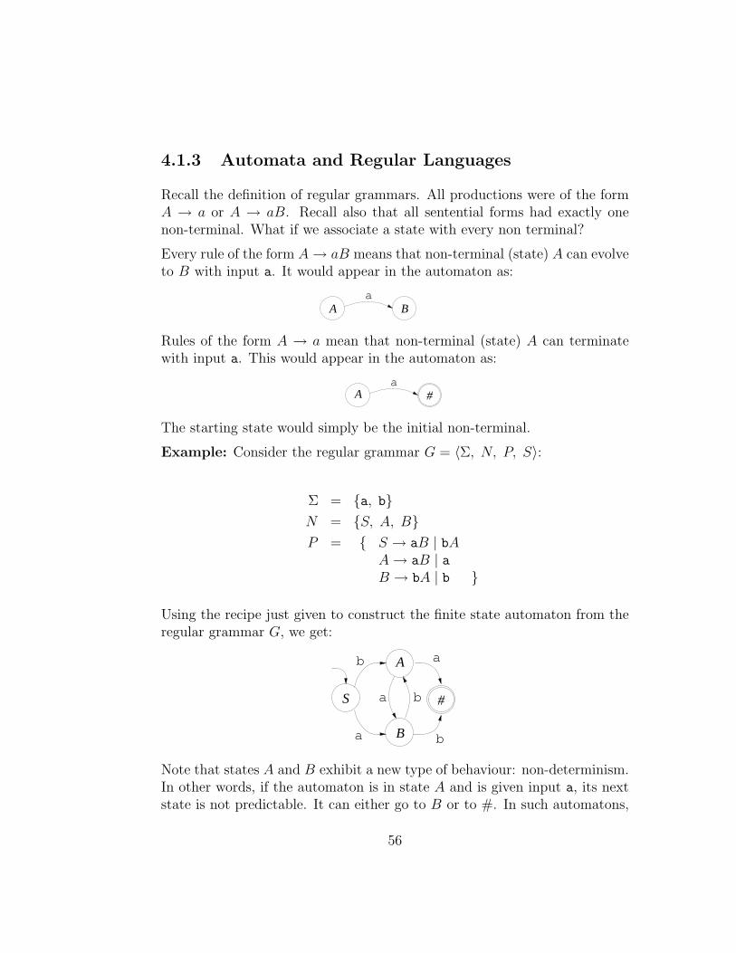
Example: Consider the regular grammar G = 〈Σ, N, P, S〉:

Σ = {a, b}N = {S, A, B}P = { S → aB | bA

A → aB | aB → bA | b }

Using the recipe just given to construct the finite state automaton from theregular grammar G, we get:

S

B

Ab a

ba

ba #

Note that states A and B exhibit a new type of behaviour: non-determinism.In other words, if the automaton is in state A and is given input a, its nextstate is not predictable. It can either go to B or to #. In such automatons,

56

a string would be accepted if there is at least one path of execution whichends in a terminal state.

Thus, intuitively at least, it seems that every regular grammar has a corre-sponding automaton with the same language, making automatons at least asexpressive as regular grammars. Are they more expressive than that? Thenext couple of examples address this problem.

S

b

b

B

a

a

A a

b

#

Consider the finite state automaton above. Let us define a grammar suchthat the non-terminal symbols are the states.

Thus, we have a grammar G = 〈Σ, N, P, S〉, where Σ = {a, b} andN = {S, A, B, #}. What about the production rules?

Clearly, the productions S → aA | bB are in P . Similarly, so are A → aAand B → bB. What about the rest of the transitions? Clearly, once from Athe machine goes to # it has no alternative but to terminate. Thus we addA → a and similarly for B, B → b. The resulting grammar is thus:

Σ = {a, b}N = {S, A, B, #}P = { S → aA | bB

A → aA | aB → bB | b }

However, sometimes things may not be so clear. Consider:

57

S

b

b

B

a

ac

c

c

A

C

Using the same strategy as before, we construct grammar G = 〈Σ, N, P, S〉,where Σ = {a, b, c} and N = {S, A, B, C}. As for the production rules,some are rather obvious to construct:

S → aA | bBA → aA

B → bB

What about the rest? Using the same design principle as for the rules justgiven, we also give:

A → cC

B → cC

C → cC

However, C may also terminate without requiring any further input. Thiscorresponds to C → ε, where C stops getting any further input and termi-nates (no more non-terminals).

Note that all the production rules we construct, except for the ε-productions,are according to the restrictions placed for regular grammars. However, wehave already identified a method for generating a regular grammar in caseswhen we have ε-productions:

1. Notice that in P , ε is derivable from the non-terminal C only.

2. We now construct the grammar G′ where we copy all rules in P butwhere we also copy the rules which use C without it:

58

S → aA | bBA → aA | cC | cB → bB | cC | cC → cC | c

3. The grammar is now regular. (Note that in some cases it may havebeen necessary modify this grammar, had we ended with one in whichwe have the rule S → ε and S also appears on the right hand side ofsome rules)

Thus it seems possible to associate a regular grammar with every automaton.This informal reasoning thus suggests that automata are exactly as expressiveas regular grammars. That is what we now set out to prove.

4.2 Deterministic Finite State Automata

We start by formalizing deterministic finite state automata. This is the classof all automata as already informally discussed, except that we do not allownon-deterministic edges. In other words, there may not be more that oneedge leaving any state with the same label.

Definition: A deterministic finite state automaton M , is a 5-tuple:

M = 〈K, T, t, k1, F 〉K is a finite set of statesT is the finite input alphabett is the partial transition function which, given a state and

an input, determines the new state: K × T → Kk1 is the initial state (k1 ∈ K)F is the set of final (terminal) states (F ⊆ K)

Note that t is partial, in that it is not defined for certain state, input combi-nations.

Definition: Given a transition function t (type K × T → K), we define itsstring closure t∗ (type K × T ∗ → K) as follows:

59

t∗(k, ε)def= k

t∗(k, as)def= t∗(t(k, a), s) where a ∈ T and s ∈ T ∗

Intuitively, t∗(k, s) returns the last state reached upon starting the machinefrom state k with input s.

Proposition: t∗(A, xy) = t∗(t∗(A, x), y) where x, y ∈ T ∗.

Definition: The set of strings (language) accepted by the deterministic finitestate automaton M is denoted by T (M) and is the set of terminal strings x,which, when M is started from state k1 with input x, it finishes in one of thefinal states. Formally it is defined by:

T (M)def= {x | x ∈ T ∗, t∗(k1, x) ∈ F}

Definition: Two deterministic finite state automata M1 and M2 are said tobe equivalent if they accept the same language: T (M1) = T (M2).

Example: Consider the automaton depicted below:

BS

a

b

a

A

Formally, this is M = 〈K, T, t, S, F 〉 where:

K = {S, A, B}T = {a, b}t = {(S, a) → A, (A, a) → B, (A, b) → S}

F = {B}

We now prove that every string of the form a(ba)na (where n ≥ 0) is gener-ated by M .

We require to prove that {a(ba)na | n ≥ 0} ⊆ T (M)

We first prove that t∗(S, a(ba)n) = A by induction on n.

Base case (n = 0): t∗(S, a) = t(S, a) = A.

60

Inductive case: Assume that t∗(S, a(ba)k) = A.

t∗(S, a(ba)k+1)= t∗(S, a(ba)kba)= t∗(t∗(S, a(ba)k), ba) by property of t∗= t∗(A, ba) by inductive hypothesis= A by applying t∗

Completing the induction. Hence, for any n:

t∗(S, a(ba)na) = t(t∗(S, a(ba)n), a) = t(A, a) = B ∈ F

Hence a(ba)na ∈ T (M).

Proposition: For any deterministic finite state automaton M , we can con-struct an equivalent finite state automaton M ′ with a total transition func-tion.

Strategy: We add a new dummy state ∆ (and is not a final state) to whichall previously ‘missing’ arrows point.

Proof: Define deterministic finite state machine M ′ as follows: M ′ = 〈K ∪{∆}, T, t′, k1, F 〉 where t′(k, x) = t(k, x) whenever t(k, x) is defined,t′(k, x) = ∆ otherwise.

Part 1: T (M) ⊆ T (M ′)

Consider x ∈ T (M). This implies that t∗(k1, x) ∈ F . But by definition,whenever t∗ is defined, so is t′∗. Furthermore they give the same value, andthus t′∗(k1, x) = t∗(k1, x) ∈ F . Hence x ∈ T (M ′).

Part 2: T (M ′) ⊆ T (M)

We start by proving, by induction on the length of x that, if t′∗(A, x) ∈ Fthen t∗(A, x) ∈ F .

Base case (|x| = 0): Implies that A ∈ F and x = ε. Hence t∗(A, x) ∈ F .

Inductive case: Assume that the argument holds for |x| = k. Now considerx = ay, where |x| = k + 1 and a ∈ T .

Notice that t′∗(A, ay) = t′∗(t′(A, a), y). Hence, by induction hypothesis

t∗(t′(A, a), y) ∈ A. But t′(A, a) 6= ∆ (otherwise t∗ would not be defined on

it), and therefore t(A, a) = t′(A, a).

Therefore, t∗(t(A, a), y) ∈ A, implying that t∗(A, ay) ∈ A completing theinduction.

61

Therefore, by this result t′∗(k1, x) ∈ F implies that t∗(k1, x) ∈ F . Hencex ∈ T (M ′) implies that x ∈ T (M), completing the proof.

�

Example: Consider the automaton given in the previous example.

BS

a

b

a

A

We can define a automaton M ′ with a total transition function equivalent toM by using the method just prescribed in the previous theorem.

Formally, this would be M ′ = 〈K ′, T, t′, S, F 〉 where:

K ′ = {S, A, B, ∆}T = {a, b}t′ = { (S, a) → A,

(S, b) → ∆,(A, a) → B,(A, b) → S,(B, a) → ∆,(B, b) → ∆,(∆, a) → ∆,(∆, b) → ∆ }

F = {B}

This can be visually represented by:

BS

a

b

a

A

∆b

b

a

ab

62

4.2.1 Implementing a DFSA

Given the transition function of a finite state automaton, we can draw up atable of state against input symbol and fill in the next state.

a a . . .

A t(A, a) t(B, a) . . .B t(A, b) t(B, b) . . ....

......

. . .

Combinations of state against input for which the transition function is un-defined, are left empty.

Example: Consider the following automaton:

S

B

Ab

a

ba #

c

c

The transition function of this automaton is:

a b c

S B AA B #B A ##

Adding a dummy state ∆ to make the transition function total is verystraightforward:

a b c

S B A ∆A B ∆ #B ∆ A ## ∆ ∆ ∆∆ ∆ ∆ ∆

Visually, the automaton with a total transition function would look like:

63

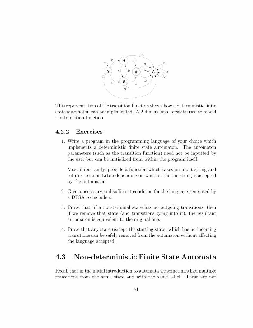
S

B

Ab

a

ba #

a

b

c

c

cb

c

a

b

c

a

∆

This representation of the transition function shows how a deterministic finitestate automaton can be implemented. A 2-dimensional array is used to modelthe transition function.

4.2.2 Exercises

1. Write a program in the programming language of your choice whichimplements a deterministic finite state automaton. The automatonparameters (such as the transition function) need not be inputted bythe user but can be initialized from within the program itself.

Most importantly, provide a function which takes an input string andreturns true or false depending on whether the the string is acceptedby the automaton.

2. Give a necessary and sufficient condition for the language generated bya DFSA to include ε.

3. Prove that, if a non-terminal state has no outgoing transitions, thenif we remove that state (and transitions going into it), the resultantautomaton is equivalent to the original one.

4. Prove that any state (except the starting state) which has no incomingtransitions can be safely removed from the automaton without affectingthe language accepted.

4.3 Non-deterministic Finite State Automata

Recall that in the initial introduction to automata we sometimes had multipletransitions from the same state and with the same label. These are not

64

deterministic finite state automata since we had defined a transition function,and thus we can have only one value for the application t(A, a). How can wegeneralize the concept of automata to allow for non-determinism?

Definition: A non-deterministic finite state automaton M is a 5-tuple〈K, T, t, k1, F 〉, where:

K is a finite set of states in which the automaton can resideT is the input alphabett1 ∈ K is the initial stateF ⊆ K is the set of final states

t is a total function from state and input to a set of states. (K × T → PK).

The set of states t(A, a) defines all possible new states if the machine readsan input a in state A. If no transition is possible, for such a state, inputcombination t(A, a) = ∅.

Example: Consider the non-deterministic automaton depicted below:

S

b

b

B

a

a

A a

b

C

This would formally be encoded as non-deterministic finite state automatonM = 〈{S, A,B,C}, {a, b}, t, S, {C}〉, where t is:

t = { (S, a) → {A},(S, b) → {B},(A, a) → {A, C},(A, b) → ∅,(B, a) → ∅,(B, b) → {B, C},(C, a) → ∅,(C, b) → ∅ }

65

Definition: The extension of a transition function to take sets of statest : PK × T → PK, is defined by:

t(S, a)def=

⋃k∈S

t(k, a)

Example: In the previous example, imagine the machine has received inputa in state A. Clearly, the new state is either A or C. Where would themachine now reside if we received another input a?

t({A, C}, a)= t(A, a) ∪ t(C, a)

= {A, C} ∪ ∅= {A, C}

Definition: As before, we can now define t∗, the string closure of t:

t∗(S, ε)def= S

t∗(S, as)def= t∗(t(S, a), s) where a ∈ T and s ∈ T ∗

Definition: A non-deterministic finite state automaton M is said to accepta terminal string s, if, starting from the initial state with input s, it mayreach a final state: t∗(k1, s) ∩ F 6= ∅.Definition: The language accepted by a non-deterministic finite state au-tomaton M , is the set of all strings (in T ∗) accepted by M :

T (M)def= {s | s ∈ T ∗, t∗(k1, s) ∩ F 6= ∅}

How does the class of languages accepted by non-deterministic finite stateautomata compare with those accepted by the deterministic variety, and withthose generated by context-free or regular grammars? Thus is what we nowset out to discuss.

66

4.4 Formal Comparison of Language Classes

Implementation of a non-deterministic finite state automaton using a com-puter language is not as simple as writing one for a deterministic automaton.The cells in the transition table would have to hold lists of states, rather thanjust one state. Checking whether a string is accepted or not is also not assimple, since a ‘wrong’ transition early on could mean that a terminal stateis not reached and to make sure that a string is not accepted would meanhaving to search through all the possibilities exhaustively.

This seems to indicate that non-determinism adds complexity. Does thismean, however, that there are languages which a non-deterministic finitestate automaton can accept but for which there is no deterministic finitestate automaton which accepts them? The next two theorems prove thatthis is not the case, and that (surprise, surprise!) for every non-deterministicfinite state automaton, there is a deterministic finite state automaton whichaccepts the same language (and vice-versa).

Theorem: Every language recognizable by a deterministic finite state au-tomaton is also recognizable by a non-deterministic finite state automaton.

Proof: Given a DFSA M = 〈K, T, t, k1, F 〉, build an equivalent DFSAM ′ = 〈K ′, T ′, t′, k′1, F ′〉, but in which the transition function is total.

We now define a NFSA M ′′ = 〈K ′, T ′, t′′, k′1, F ′〉, where t′′ = {(A, a) →{B} | (A, a) → B ∈ t′}.

We claim that the languages generated by M ′ and M ′′ are, in fact, identical.This can be proved by showing that the range of t′′∗ is in fact singleton setsand that t′′∗(A, a) = {B} ⇔ t′∗(A, a) = B. This is easily provable by inductionand will not be done here.

Now, consider x ∈ T (M ′). This is implies that t′∗(A, x) = B and B ∈ F .Hence, by the above reasoning, t′′∗(A, x) = {B} and {B} ∈ F , which in turnimplies that t′′∗(A, x) ∩ F 6= ∅. Thus, x ∈ T (M ′′).

Conversely, if x ∈ T (M ′′), t′′∗(A, x) ∩ F 6= ∅. But t′′∗(A, x) = {B}, whichimplies that {B} ∩ F 6= ∅, that is B ∈ F . But t′′∗(A, x) = {B} also implies(by the above reasoning) that t′∗(A, x) = B. Hence t′∗(A, x) ∈ F . x ∈ T (M ′).

Thus, T (M ′) = T (M ′′).�

67

Theorem: Conversely, if a language is recognizable by a non-deterministicfinite state automaton, there is a deterministic finite state automaton whichrecognizes the language.

Strategy: The idea is to create a new automaton with every combinationof states in the original represented in the new automaton by a state. Thus,if the original automaton had states A and B, we now create an automatonwith 4 states labeled ∅, {A}, {B} and {A, B}. The transitions would thencorrespond directly to t. Thus, if t({A}, a) = {A, B} in the original automa-ton, we would have a transition labeled a from state {A} to state {A, B}.The equivalence of the languages is then natural.

Proof: Given a DFSA M = 〈K, T, t, k1, F 〉, we now define a NFSAM ′′ = 〈K ′, T, t′, k′1, F ′〉, where :

K ′ = PK

t′ = t

k′1 = {k1}F ′ = {S | S ⊆ K, S ∩ F 6= ∅}

x ∈ T (M)

⇔ by definition of T (M)

t∗({k1}, x) ∩ F 6= ∅⇔ by definition of F ′

t∗({k1}, x) ∈ F ′

⇔ by definition of T (M ′)

x ∈ T (M ′)

�

Example: Consider the non-deterministic finite state automaton below:

S

a

a

#

68

To produce a deterministic finite state automaton with the same language, weneed a state for every combination of original states. Thus, we will now havethe states ∅, {S}, {#} and {S, #}. The starting state is {S}, whereas thefinal states are all those which include # ({#} and {S, #}). By constructingt, we can now construct the desired automaton:

{S,#}

{#}

φ

a

{S}

a

a

a

Example: For a slightly more complicated example, consider the non-deterministic finite state automaton below:

S

B

A

#

b

a

b a

b

a

Since, for any finite set of size n, its power set is of size 2n, we will now have24 or 16 states!

To simplify the presentation we constrain the automaton by leaving out stateswhich are unreachable from the starting state ({S, A}, {S, B, A} etc), andstates from which no terminal state is reachable (∅).You can check out for yourselves that the deterministic automaton below isdefined according to the rules set in the last theorem:

{B,#}{S}

{A}

{B} {A,#}

a b

ab

b

a

This method provides a simple way of implementing a non-deterministic finitestate automaton . . . by first obtaining an equivalent deterministic one. As

69

the last example indicates, the number of states in the deterministic growspretty quickly even for small numbers of states in the original. A transformed10 state non-deterministic automaton would have over 1000 states. A 20state one would end up with more that 1,000,000 states! This indicatesthe importance of methods to reduce the size of automatons by removingirrelevant states. Some simple results were presented in the exercises ofsection 4.2.2, but this is beyond the scope of this course and will not bediscussed any further here.

We still have not answered the question of how the languages generatedby these automata relate to context-free and regular automata. The nexttheorem should answer this.

Theorem: Non-deterministic finite state automata, deterministic finite stateautomata and regular grammars generate exactly the same class of languages.The following statements are equivalent:

1. L is a regular language

2. L is accepted by a non-deterministic finite state automaton

3. L is accepted by a deterministic finite state automaton

Strategy: (2) and (3) have already been proved equivalent. In the intro-ductory part of this chapter we presented a strategy for obtaining a (non-deterministic) automaton from a regular grammar and vice-versa. These arethe methods which will be formalized here.

Proof: By the previous two theorems, we know that (2)⇔(3). We now showhow that (3)⇒(1) and that (1)⇒(2). This will complete the proof thanks totransitivity of implication.

Part 1: (3)⇒(1). Let L be the language generated by deterministic finitestate automaton M = 〈K, T, t, k1, F 〉. Now consider the regular grammarG = 〈T, K, P, k1〉, where P is defined by:

Pdef= {A → aB | t(A, a) = B}

∪ {A → a | t(A, a) ∈ F}

Claim: This generates L \ {ε}.

70

This can be proved by induction on the length of the derivation on thestatements:

k1+⇒G aA ⇔ t∗(k1, a) = A

k1+⇒G a ⇔ t∗(k1, a) ∈ F

If ε ∈ L we can add this to the regular language using techniques alreadydiscussed.

Part 2: (1)⇒(2). Given grammar G = 〈Σ, N, P, S〉, we define the non-deterministic automaton M = 〈N ∪ {#}, Σ, t, S, {#}〉, where t is definedby:

t(A, a)def= {B | A → aB ∈ P}

∪ {# | A → a ∈ P}

This produces L(M) \ {ε}.If ε is in L, we need to add ε to the language accepted by M . This is doneby defining M ′ = 〈N ∪ {#, k1}, Σ, t′, k1, {#, k1}〉, where t′ is defined as:

t′(k1, a)def= t(S, a)

t′(A, a)def= t(A, a) if A 6= k1

In other words, we add a new initial (and final) state k1. This obviously addsthe desired ε. How about the other inputs? State k1 will also have outgoingtransitions like S. This avoids problems with any arrows going back into S.

�

These equivalences will not be proved during the course. Our aim is mainlyto show the important results in this particular area of computer science andthe application of basic techniques. These proofs should be within your grasp.If you are interested in the details, the textbooks should provide adequateinformation.

This is one of the major results of the course. Most importantly, you shouldbe able to transform between the three classes, including the special cases.

71

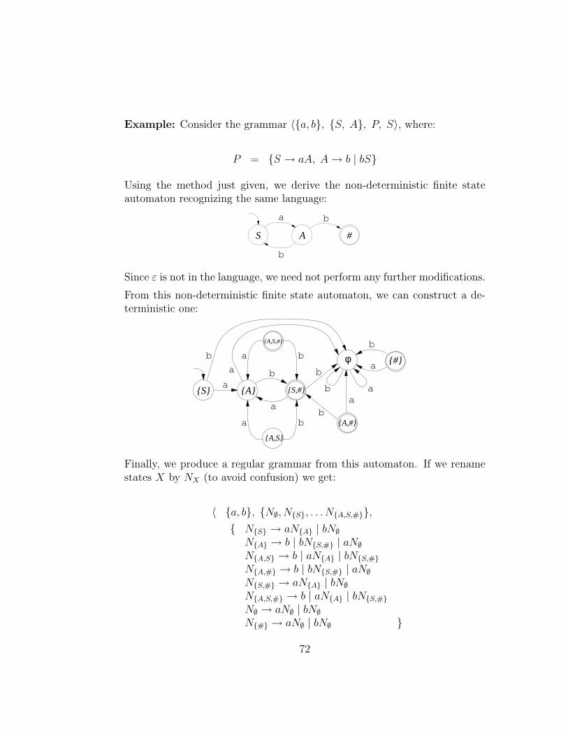
Example: Consider the grammar 〈{a, b}, {S, A}, P, S〉, where:

P = {S → aA, A → b | bS}

Using the method just given, we derive the non-deterministic finite stateautomaton recognizing the same language:

S

a

b

A

b

#

Since ε is not in the language, we need not perform any further modifications.

From this non-deterministic finite state automaton, we can construct a de-terministic one:

b

a

a

a

a b

b

{S}

a

b

{A,S,#}

{A} {S,#}

{A,#}

{#}

{A,S}

b

b a

a

ab

bφ

Finally, we produce a regular grammar from this automaton. If we renamestates X by NX (to avoid confusion) we get:

〈 {a, b}, {N∅, N{S}, . . . N{A,S,#}},{ N{S} → aN{A} | bN∅

N{A} → b | bN{S,#} | aN∅N{A,S} → b | aN{A} | bN{S,#}N{A,#} → b | bN{S,#} | aN∅N{S,#} → aN{A} | bN∅N{A,S,#} → b | aN{A} | bN{S,#}N∅ → aN∅ | bN∅N{#} → aN∅ | bN∅ }

72

N{S}〉

Applying the methods used in the theorems, we are guaranteed that theinitial and final grammars are equivalent.

Note that, to make the resultant grammar smaller, we can remove redundantstates at the DFSA stage or unused non-terminals in the regular grammarstage. If we choose to make the DFSA more efficient, we note that the(non-initial) states {A, S, #}, {A, S}, {A, #} and {#} have no in-comingtransitions and can thus be left out. ∅ cannot evolve to any terminal state(for any number of moves) and can thus also be left out. The resultant DFSAwould now look like:

b

a

a{S} {A} {S,#}

The resulting smaller grammar would then be:

〈 {a, b}, {N{S}, N{A}, N{S,#}},{ N{S} → aN{A}

N{A} → b | bN{S,#}N{S,#} → aN{A} }

N{S}〉

These results are very useful in the implementation of regular languageparsers. Given a regular language (or rather grammar), we have a safe,fail-proof method of designing a deterministic finite state automaton to rec-ognize the language. Since it is particularly easy to program DFSA and checkwhether or not they accept a particular string, we can easily implement them.But the use of these theorems is not limited to implementation issues. Theycan help resolve questions about grammars by using arguments about finitestate machines (or vice-versa).

Proposition: If L is a regular language over Σ, then so is its inverse L(where L = Σ∗ \ L).

Strategy: Since L is a regular grammar, there is a deterministic finite stateautomaton M which recognizes it. We now design an automaton M identical

73

to M except that the a state S is a final state of M if and only if it is not afinal state of M . The language recognized by M is exactly L. Hence thereis a regular grammar recognizing L.

Proof: Since L is a regular language, there is a regular grammar generatingit. By the theorem above, therefore, there is a DFSA recognizing it. LetM = 〈Σ, T, t, k1, F 〉 be such a DFSA. Assume that t is total (otherwise adda dummy state).

Consider M = 〈Σ, T, t, k1, Σ \ F 〉. We claim that T (M) = Σ∗ \ T (M).

x ∈ T (M)

⇒ t∗(k1, x) ∈ Σ \ F

⇒ t∗(k1, x) /∈ F

⇒ x /∈ T (M)

⇒ x ∈ Σ \ T (M)

The reverse argument is very similar and is left out.

But Σ∗ \ T (M) = Σ∗ \ L = L and hence T (M) = L. Therefore, there is aDFSA generating L, which, using the theorem means that there is a regulargrammar generating it. Hence, L is a regular language.

�

Corollary: If L1 and L2 are regular languages, then so is L1 ∩ L2.

Proof: L1 ∩ L2 = L1 ∪ L2

�

Given these results, given two regular grammars, we can construct a regulargrammar recognizing their intersection. Just using the results we gave inthese notes, the procedure is rather lengthy but is easily automated:

1. Produce an equivalent NFSA for each of the two grammars (call themN1 and N2).

2. From the NFSA (N1 and N2) produce equivalent DFSA (call them D1

and D2).

3. Produce total DFSA (D1 and D2) recognizing the inverse of the lan-guages recognized by D1 and D2.

74

4. From D1 and D2 produce equivalent regular grammars G1 and G2.

5. Construct a regular grammar G∪ recognizing the union of the grammarsG1 and G2.

6. Produce a NFSA N∪ equivalent to G∪.

7. Produce a total DFSA D∪ equivalent to N∪.

8. From D∪ produce D∪ which recognizes the inverse of the language.

9. Construct a regular grammar G from DFSA D∪.

The process may be lengthy and boring but it is guaranteed to work. In mostcases, this process will produce an unnecessarily large grammar. However,as already mentioned, efficiency is not an issue which we will be looking into.

Example: Construct a grammar to recognize the inverse of the languagegenerated by:

〈{a, b}, {S, A}, {S → aA | bA, A → a | aS}, S〉

The non-deterministic finite state automaton we construct is:

aaa

bS A #

Note that ε is not in the language we derive and this NFSA does not requireany modification. From this we generate the 8-state DFSA:

a

ba

a

b

a

b b

a

b

a

a

b

ba

b

{S,#}

φ

{S,A,#}{S,A}

{#} {A,#}

{A}{S}

This is optimized and made total to:

75

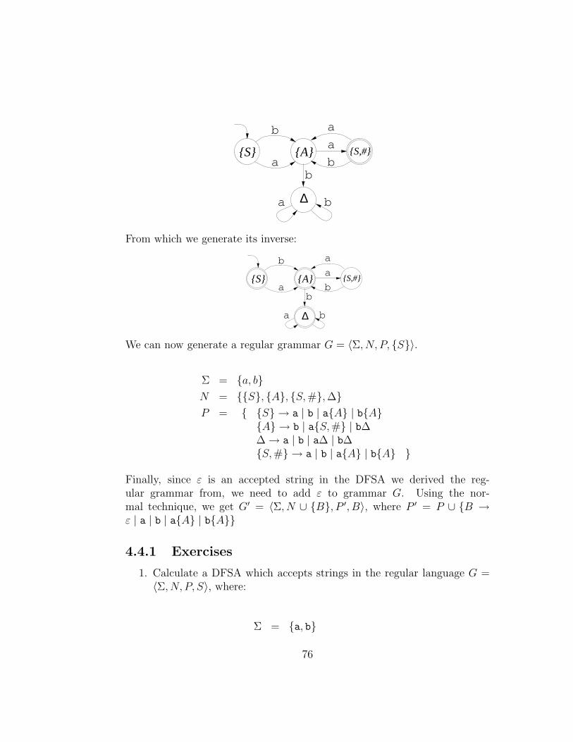
a

ba

a

b{S} {A} {S,#}

∆

b

a b

From which we generate its inverse:

a

ba

a

b{S} {A} {S,#}

b

∆a b

We can now generate a regular grammar G = 〈Σ, N, P, {S}〉.

Σ = {a, b}N = {{S}, {A}, {S, #}, ∆}P = { {S} → a | b | a{A} | b{A}

{A} → b | a{S, #} | b∆∆ → a | b | a∆ | b∆{S, #} → a | b | a{A} | b{A} }

Finally, since ε is an accepted string in the DFSA we derived the reg-ular grammar from, we need to add ε to grammar G. Using the nor-mal technique, we get G′ = 〈Σ, N ∪ {B}, P ′, B〉, where P ′ = P ∪ {B →ε | a | b | a{A} | b{A}}

4.4.1 Exercises

1. Calculate a DFSA which accepts strings in the regular language G =〈Σ, N, P, S〉, where:

Σ = {a, b}

76

N = {S, A,B}P = { S → aA | bB

A → bS | bB → aS | a }

2. Construct a grammar G′ which accepts L(G) ∪ {ε}, where G is asdefined in the previous question. From G′ construct a NFSA whichrecognizes the same language.

3. Construct a DFSA which recognizes L(G), where G is the regular gram-mar G = 〈Σ, N, P, S〉, where:

Σ = {a, b}N = {S, A,B}P = { S → aB | aA

A → bS | bB → aA | a }

77

Chapter 5

Regular Expressions

This chapter discusses another way of defining a language — by using reg-ular expressions. This notation is particularly adept at describing simplelanguages in a concise and readable way. It is used in certain text editors(for example, vi) to specify a search for a particular sequence of symbols inthe text. A similar notation is also used to specify the acceptable syntax ofcommand lines.

5.1 Definition of Regular Expressions

Definition: A regular expression over an alphabet Σ takes the form of oneof the following:

• 0

• 1

• a (where a∈ Σ)

• (e) (where e is a regular expression)

• e∗ (where e is a regular expression)

• e+ (where e is a regular expression)

• e1 + e2 (where both e1 and e2 are regular expressions)

78

• e1e2 (where both e1 and e2 are regular expressions)

Thus, for example, all the following are regular expressions over the alphabet{a, b}:

• (a + b)∗

• a∗b∗

• (ab + ba)+

• ab∗c

Definition: Given a regular expression e, we can recursively define thelanguage it recognizes E(e) using:

• E(0)def= ∅

• E(1)def= {ε}

• E(a)def= {a}

• E((e))def= E(e)

• E(e∗)def= E(e)∗

• E(e+)def= E(e)+

• E(e1 + e2)def= E(e1) ∪ E(e2)

• E(e1e2)def= E(e1)E(e2)

Let us consider the languages generated by the previous examples:

• E((a + b)∗): Note that E(a + b) = {a, b}. Thus the language acceptedby the expression is {a, b}∗ — which is the set of all strings over thealphabet {a, b}.

• E(a∗b∗): By definition, E(a∗) is the set of all (possibly empty) sequencesof a. Hence, the expression accepts strings of the form an or bn.

79

• E((ab+ ba)+) is the set of all strings built from sequences of ab or ba.

• E(ab∗c) = {abnc | n ≥ 0}

Although these language derivations have been presented informally, theycan very easily be proved formally from the definitions just given.

5.2 Regular Grammars and Regular Expres-

sions

One immediate result of these definitions and the theorems we have alreadyproved about regular languages, is that regular grammars are at least asexpressive as regular expressions. In other words, every language generatedby a regular expression is regular.

Proposition: For any regular expression e, E(e) is a regular language.

Proof: The proof proceeds by structural induction over the syntax of ex-pression e:

Base cases:

• E(0) is a regular language since there is a regular grammar producingit (namely a regular grammar with no production rules)

• E(1) is a regular language, since it is generated by 〈Σ, {S}, {S → ε}, S〉,which is a regular grammar.

• For any terminal symbol a, E(a) is a regular language, produced by〈{a}, {S}, {S → a}, S〉.

Inductive cases: Assume that the property holds of regular expressions e1

and e2 (that is, for both of them E(ei) is a regular language).

• E((e1)) is the same as E(e1) and is thus a regular language.

• E(e∗1) is defined to be (E(e1))∗. But we have proved that for any regular

language L, L∗ is also a regular language. Thus (E(e1))∗ is a regular

language and hence so is E(e∗1).

80

• As for E(e+1 ), simply note that given any regular language L, L+ is also

regular.

• Similarly, the union of two regular languages is also regular. Hence,E(e1 + e2) is a regular language.

• Finally, the catenation of two regular languages is also regular. Thus,by definition, E(e1e2) is a regular language.

�

Example: Construct a deterministic finite state automaton which acceptsthe regular expression: 1 + a(ab)∗b:

F

S A

B

b

a

b

a

It is usually quite easy to construct a deterministic automaton, however, itis also easy to make a simple mistake. The theorems we already presentedshould ideally be used to construct the automata. Thus, for example, inthe above example, we start by constructing regular grammars for the basicregular expressions (a, b, 1) using the method described in the last theorem.We would then proceed to construct the regular grammar for the union ofa and b, which we then use to construct another grammar recognizing itsKleene closure (a + b)∗. We then use the catenation theorem to add prefixa and postfix b and finally add ε to the language (or use the union theoremto add 1. This grammar is then converted to a DFSA via a NFSA.

As in other cases, this looks like an awful lot of boring work! However, it isimportant to realize that this can all be easily automated.

The next question arising is whether there are regular languages which cannotbe expressed as regular expressions. This was shown not to be the case byKleene. This, together with the previous proposition imply that regularlanguages and regular expressions are equally expressive.

Theorem: Every regular language can be expressed as a regular expression.

Strategy: The idea is to start off from a DFSA (recall that regular gram-mars and DFSA recognize exactly the same class of languages). This isdecomposed into a number of automata, each of which has exactly one final

81

state. We then prove (non-trivially) that such automata can be expressed asregular expressions.

Proof: Let L be a regular grammar. Then, there is a deterministic finitestate automaton M , where T (M) = L, where M = 〈K, T, t, k1, F 〉:

K = {k1, k2, . . . kn}F = {kλ1 , kλ2 , . . . kλm}

Now consider the machines:

Mi = 〈K, T, t, k1, {kλi}〉

Clearly, T (M) =⋃λm

i=1 T (Mi).

Thus, if we can construct a regular expression ei for each Mi, we have:

E(e1 + . . . eλm)

= E(e1) + . . . E(eλm)

=λm⋃i=1

T (Mi)

= T (M)

= L

and thus L can also be expressed as a regular expression.

Let us consider one particular Mi and rename the states such that:

K = {k1, k2, . . . kn}F = {kn}

We now define language T li,j (where 1 ≤ i, j ≤ n and 0 ≤ l ≤ n) to be the

set of all strings x satisfying:

82

1. t∗(ki, x) = kj and

2. for all proper prefixes y of x, t∗(ki, y) = {km | m ≤ l}

Informally, T li,j is thus the set of all strings which send automaton Mi from

ki to kj by only going through states in {k1 . . . kl}.The proof proceeds by induction on l, to show that T (T l

i,j is a regular lan-guage.

Base case (l = 0): We split this part into two cases: i = j and i 6= j.

• i = j: T 0i,j = E(1) if there is no a such that t(ki, a) = kj. Otherwise T 0

i,j

is simply the union of all such labels: 1 + a1 + a2 + . . . + am. In bothcases, T 0

i,j is equivalent to a regular expression.

• i 6= j: T 0i,j = E(0) if there is no a such that t(ki, a) = kj. Otherwise

T 0i,j is simply the union of all such labels: a1 + a2 + . . . + am. In both

cases, T 0i,j is equivalent to a regular expression.

Inductive case: Assume T li,j can always be expressed as a regular expres-

sion.

We now claim that T l+1i,j = T l

i,j + T li,l+1(T

ll+1,l+1)

∗T ll+1,j.

Informally, it says that the strings which take the automaton from state tito state tj through states in {k1, . . . kl+1} either:

• do not go through kl+1 and hence are also in T li,j, or

• go to kl+1 a number of times. In between these ‘visits’ kl+1 is nottraversed again. Thus, the overall trip can be expressed as a sequenceof trips from ki to kl+1, from kl+1 to kl+1 for a number of times, andfinally from kl+1 to kj, where in each of these mini-trips, kl+1 is nottraversed. Hence, the whole trip is in T l

i,l+1(Tll+1,l+1)

∗T ll+1,j.

By the inductive hypothesis, all the traversals can now be expressed as regularexpressions and thus, so can T l

i,j.

This completes the induction proof.

Now, simply note that T (Mi) = T n1,n. Hence, T (Mi) can be expressed as a

regular expression, and so can T (M).�

83

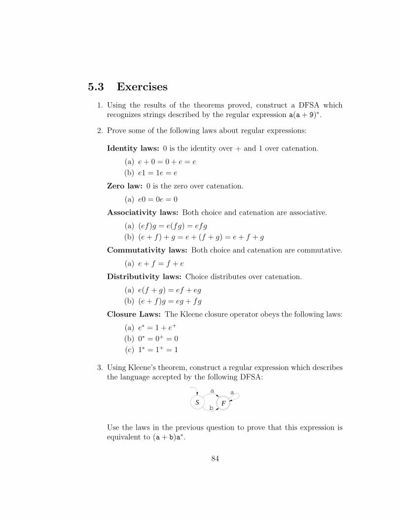
5.3 Exercises

1. Using the results of the theorems proved, construct a DFSA whichrecognizes strings described by the regular expression a(a + 9)∗.

2. Prove some of the following laws about regular expressions:

Identity laws: 0 is the identity over + and 1 over catenation.

(a) e + 0 = 0 + e = e

(b) e1 = 1e = e

Zero law: 0 is the zero over catenation.

(a) e0 = 0e = 0

Associativity laws: Both choice and catenation are associative.

(a) (ef)g = e(fg) = efg

(b) (e + f) + g = e + (f + g) = e + f + g

Commutativity laws: Both choice and catenation are commutative.

(a) e + f = f + e

Distributivity laws: Choice distributes over catenation.

(a) e(f + g) = ef + eg

(b) (e + f)g = eg + fg

Closure Laws: The Kleene closure operator obeys the following laws:

(a) e∗ = 1 + e+

(b) 0∗ = 0+ = 0

(c) 1∗ = 1+ = 1

3. Using Kleene’s theorem, construct a regular expression which describesthe language accepted by the following DFSA:

FSb

a a

Use the laws in the previous question to prove that this expression isequivalent to (a + b)a∗.

84

5.4 Conclusions

The constructive result we had proved, that regular grammars are just asexpressive as DFSA, and the ease of implementation of DFSA indicatedthe interesting possibility of implementing a program which, given a regulargrammar, constructs a DFSA to be able to efficiently deduce whether a givenstring is in the grammar or not. The question left pending was how todescribe the regular grammar. The only possibility we had was to somehowencode the production rules as text.

The first result in this chapter opened a new possibility. All regular expres-sions are in fact regular languages and we have the means to construct aregular grammar from such an expression. Can we use regular expressions todescribe regular languages? It is rather obvious that such a representation ismuch more ‘ascii-friendly’, but are we missing out on something? Are thereregular languages which are not expressible as regular expressions? The sec-ond theorem rules this out, justifying the use of regular expressions as theinput format of regular languages.

This is precisely what LEX does. Given a regular expression, LEX automat-ically generates the code to recognize whether a string is in the expressionor not and all this is done via DFSA as discussed in this course. You will bestudying further what LEX does in next year’s course on ‘Compiling Tech-niques’.

The course has, up to this point shown the equivalence of:

• Languages accepted by regular grammars

• Languages recognizable by non-deterministic finite state automata

• Languages recognizable by deterministic finite state automata

• Languages describable by regular expressions

However, we have mentioned that certain context free languages cannot berecognized by a regular grammar. In particular, there is no way of writinga regular grammar which recognizes matching parentheses. This severelylimits the use of regular grammars in compiler writing. We thus now try toreplicate similar work to that we have just done on regular languages but

85

on context free languages. Is there a machine which we can construct froma context free grammar which easily checks whether a string is accepted ornot? Can this conversion be automated? These are the questions we willnow be asking.

If you are wondering what is the use of LEX in compiler writing if LEXrecognizes only regular languages and regular languages are not expressiveenough in compiler writing, the answer is that compilers perform at least twopasses over the text they are given. The first, so called lexical analysis simplyidentifies tokens such as while or :=. The job of the lexical analyzer is togroup together such symbols to simplify the work of the parser, which checksthe structure of the tokens (for example while if would make no sense inmost languages). The lexical analysis can usually be readily performed bya regular grammar, whereas the parser would need to use a context-freelanguage.

86

Chapter 6

Pushdown Automata

The main problem with finite state automata, is that they have no way of‘remembering’. Pushdown automata are basically an extension of finite stateautomata, which allows for memory. The extra information is carried aroundin the form of a stack.

6.1 Stacks

A stack is a standard data structure which is used to store information to beretrieved at a later stage. A stack has an underlying data type Σ, such thatall information placed on the stack if of that type. Two operations can beused on a stack:

Push: The function push takes a stack of underlying type Σ and a value oftype Σ and returns a new stack which is identical to the original butwith the given value on top.

Pop: The function pop takes a non-empty stack and returns the value on topof the stack. The stack is also returned with the top value removed.

We will use strings to formally define stacks. ε is the empty stack, whereasany string over Σ is a possible configuration of a stack with underlying typeΣ. The functions on stacks are formalized as follows:

87

push : StackΣ × Σ → StackΣ

push(s, a)def= sa

pop : StackΣ → Σ× StackΣ

pop(as)def= (a, s)

6.2 An Informal Introduction

A pushdown automaton has a stack which it uses to store information. Uponinitialization, the stack always starts off with a particular value being pushed(normally used to act as a marker that the stack is about to empty). Everytransition now depends not only on the input, but also on the value on thetop of the stack. Upon performing a transition, a number of values may alsobe pushed on the stack. In diagrams, transitions are now marked as shownin the figure below:

(p,a)/x

The label (p, a)/x is interpreted as follows: pop a value off the stack, if thesymbol just popped is p and the input is a, then perform the transition andpush onto the stack the string x. If the transition cannot take place, tryanother using the value just popped. The machine ‘crashes’ if it tries to popa value off an empty stack.

The arrow marking the initial state is marked by a symbol which is pushedonto the stack at initialization.

As in the case of FSA, we also have a number of final states which are usedto determine which strings are accepted. A string is accepted if, starting themachine from the initial state, it terminates in one of the final states.

Example: Consider the PDA below:

88

S’

(a,a)/aa

(a,b)/( , )/

(a,b)/( ,a)/a

E

S

Initially, the value ⊥ is pushed onto the stack. This will be called the ‘bottomof stack marker’. While we are at the initial state S, read an input. If it isa push back to the stack whatever has just been popped, together with anextra a. In other words, the stack now contains as many as as have beenaccepted.

When a b is read, the state now changes to S ′. The top value of the stack(a) is also discarded. While in S ′ the PDA continues accepting bs as longas there are as on the stack. When finally, the bottom of stack marker isencountered, the machine goes to the final state E.

Hence, the machine is accepting all strings in the language {anbn | n ≥1}. Note that this is also the language of the context free grammar withproduction rules: S → ab | aSb.Recall that it was earlier stated that this language cannot be accepted by aregular grammar. This seems to indicate that we are on the right track andthat pushdown automata accept certain languages for which no finite stateautomaton can be constructed to accept.

6.3 Non-deterministic Pushdown Automata

Definition: A non-deterministic pushdown automaton M is a 7-tuple:

M = 〈K, T, V, P, k1, A1, F 〉K = a finite set of statesT = the input alphabet of MV = the stack alphabetP = transition function of M with type:

(K × V × (T ∪ {ε}) → P(K × V ∗)k1 ∈ K is the start stateA1 ∈ V is the initial symbol placed on the stackF ⊆ K is the set of final states

89

Of these, the production rules (P ) may need a little more explaining. P isa total function such that P (k, v, i) = {(k′1, s1), . . . (k

′n, sn)}, means that: in

state k, with input i (possibly ε meaning that the input tape is not inspected)and with symbol v on top of the stack (which is popped away), M can evolveto any of a number of states k′1 to k′n. Upon transition to k′i, the string si ispushed onto the stack.

Example: The PDA already depicted is formally expressed by:

M = 〈{S, S ′, E}, {a, b}, {a, b,⊥}, P, S,⊥, {E}〉

where P is defined as follows:

P (S,⊥, a) = {(S, a⊥)}P (S, a, a) = {(S, aa)}P (S, a, b) = {(S ′, ε)}P (S ′, a, b) = {(S ′, ε)}P (S,⊥, ε) = {(E, ε)}P (X, x, y) = ∅ otherwise

Note that this NPDA has no non-deterministic transitions, since every state,input, stack value triple has at most one possible transition.

Whereas before, the current state described all the information needed aboutthe machine to be able to deduce what it can do, we now also need the currentstate of the stack. This information is called the configuration of the machine.

Definition: The set of configurations of M is the set of all pairs (state,string): K × V ∗.

We would now like to define which configurations are reachable from whichconfigurations. If there is a final state in the set of configurations reachablefrom (k1, A1) with input s, s would then be a string accepted by M .

Definition: The transition function of a PDA M , written tM is a function,which given a configuration and an input symbol, returns the set of states inwhich the machine may terminate with that input.

90

tM : (K × V ∗)× (T ∪ {ε}) → K × V ∗

tM((k, xX), a)def= {(k′, yX) | (k′, y) ∈ P (k, x, a)}

Definition: The string closure transition function of a PDA M , written t∗Mis the function, which given an initial configuration and input string, returnsthe set of configurations in which the automaton may end up in after usingup the input string.

t∗M : (K × V ∗)× (T ∪ {ε}) → P(K × V ∗)

We start by defining the function for an empty stack:

t∗M((k, ε), ε)def= {(k, ε)}

t∗M((k, ε), a)def= ∅

For a non-empty stack, and input a1 . . . an, (where each ai ∈ T ∪ {ε}, weneed to find

t∗M((k,X), w)def= {(k′, X ′) |

∃a1, . . . an : T ∪ {ε} · w = a1 . . . an

∃c1, . . . cn : K × V ∗ ·c1 ∈ tM((k,X), a1)

ci+1 ∈ tM(ci, ai) for all i

(k′, X ′) ∈ tM(cn, an)

We say that c′ = (k′, X ′) is reachable from c = (k,X) by a if c′ ∈ t∗M(c, a).

Definition: The language recognized by a non-deterministic pushdown au-tomaton M = 〈K, T, V, P, k1, A1, F 〉, written as T (M) is defined by:

T (M)def= {x | x ∈ T ∗, (F × V ∗) ∩ t∗M((k1, A1), x) 6= ∅}

91

Informally, there is at least one configuration with a final state reachablefrom the initial configuration with x.

Example: Consider the following NPDA:

(a,a)/

( , )/

( ,a)/a( ,b)/b(a,a)/aa(b,b)/bb(b,a)/ab(a,b)/ba

(b,b)/(a,a)/(b,b)/

k k

k

2

3

1

This automaton accepts non-empty even-length palindromes over a, b.

Now consider the acceptance of baab:

(k1,⊥)

↓ b(k1, b⊥)

↓ a(k1, ab⊥)

↙ a ↘ a

(k1, aab⊥) (k2, b⊥)

↓ b ↓ b(k1, baab⊥) (k2,⊥)

↓ ε

(k3, ε)

From (k1,⊥), we can only reach (k1, b⊥) with b, from where we can onlyreach (k1, ab⊥) with a. Now, with input a, we have a choice. We can eitherreach (k1, aab⊥) or (k2, b⊥). In terms of the machine, it may be seen as ifit is not yet clear whether we have started reversing the word or whether weare still giving the first part of the string. The tree above shows how thedifferent alternatives branch up the tree.

92

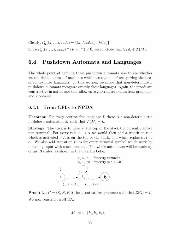
Clearly, t∗M((k1,⊥), baab) = {(k1, baab⊥), (k3, ε)}.

Since t∗M((k1,⊥), baab) ∩ (F × V ∗) 6= ∅, we conclude that baab ∈ T (M).

6.4 Pushdown Automata and Languages

The whole point of defining these pushdown automata was to see whetherwe can define a class of machines which are capable of recognizing the classof context free languages. In this section, we prove that non-deterministicpushdown automata recognize exactly these languages. Again, the proofs areconstructive in nature and thus allow us to generate automata from grammarsand vice-versa.

6.4.1 From CFLs to NPDA

Theorem: For every context free language L there is a non-deterministicpushdown automaton M such that T (M) = L.

Strategy: The trick is to have at the top of the stack the currently activenon-terminal. For every rule A → α we would then add a transition rulewhich is activated if A is on the top of the stack, and which replaces A byα. We also add transition rules for every terminal symbol which work bymatching input with stack contents. The whole automaton will be made upof just 3 states, as shown in the diagram below:

k3

( , )/S ( , )/

k k21

(A, )/α(a,a)/

for every rule αAfor every terminal a

Proof: Let G = 〈Σ, N, P, S〉 be a context free grammar such that L(G) = L.

We now construct a NPDA:

M = 〈 {k1, k2, k3},

93

Σ,

Σ ∪N ∪ {⊥},PM ,

k1,

⊥,

{k3}〉

where PM is:

• From the initial state k1 we push S and go to k2 immediately.

P ((k1,⊥), ε) = (k2, S⊥)

• Once we reach the bottom of stack marker in k2 we can terminate.

P ((k2,⊥), ε) = (k3, ε)

• For every non-terminal A in N with at least one production rule in Pof the form A → α we add the rule:

P ((k2, A), ε) = {(k2, α) | A → α ∈ P}

• For every terminal symbol a in Σ we also add:

P ((k2, a), a) = {(k2, ε)}

We now prove that T (M) = L.

The proof is based on two observations:

1. S∗⇒G xα is a leftmost derivation ⇔ (k2, α⊥) ∈ t((k1,⊥), x)

This can be proved by induction on the length of the derivation orproduction.

94

2. (t3, α) ∈ t((k1,⊥), x) ⇒ α = ε

x ∈ L

⇔ x ∈ L(G)

⇔ S∗⇒G x

⇔ (k2,⊥) ∈ t((k1,⊥), x)

⇔ (k3, ε) ∈ t((k1,⊥), x)

⇔ (k3 × V ∗) ∩ t((k1,⊥), x) 6= ∅⇔ (F × V ∗) ∩ t((k1,⊥), x) 6= ∅⇔ x ∈ T (M)

�

Example: Consider the grammar G = 〈{a, b}, {S}, {S → ab | aSb}, S〉.From this we can construct the PDA:

k3

( , )/S ( , )/

(b,b)/(a,a)/(S, )/ab(S, )/aSb

k k21

Example: Consider a slightly more complex example, with grammar G =〈{a, b}, {S, A,B}, P, S〉, where P is:

S → A | BA → aSa | aB → bSb | b

Clearly, G recognizes all palindromes over a and b except for ε. Constructinga NPDA with the same language we get:

95

k3

( , )/S ( , )/

(A, )/aSa(A, )/a(B, )/bSb(B, )/b

(S, )/A(S, )/B

(a,a)/(b,b)/

k k21

6.4.2 From NPDA to CFGs

We would now like to prove the inverse: that languages produced by NPDAare all context free languages. Before we prove the result, we prove a lemmawhich we will use in the proof.

Lemma: For every NPDA M , there is an equivalent NPDA M ′ such that:

1. M ′ has only one final state

2. the final state is the only one in which the state can be clear

3. the automaton clears the stack upon termination

Strategy: The idea is to add a new bottom of stack marker which is pushedonto the stack before M starts. Whenever M terminates we go to a newstate which can clear the stack.

Proof: Let M = 〈K, T, V, P, k1, A1, F 〉.

Now construct M ′ = 〈K ′, T, V ′, P ′, k′1,⊥, F ′〉:

K ′ = K ∪ {k′1, k′2}V ′ = K ∪ {⊥}P ′ = P

∪ {((k′1,⊥), ε) → {(k1, A1⊥)}∪ {((k,A), ε) → {(k′2, ε)} | k ∈ F, A ∈ V ′}∪ {((k′2, A), ε) → {(k′2, ε)} | A ∈ V ′}

F ′ = {k′2}

96

Note that throughout the execution of M , the stack can never be empty,since there will be, at least ⊥ left on the stack.

The proof will not be taken any further here. Check in the textbooks if youare interested in how the proof is then completed.

�

Example: Given the NPDA below we want to construct a NPDA satisfyingthe constraints motioned in the lemma.

( ,a)/a( ,b)/b(a,a)/aa(b,b)/bb

(a,b)/

S

E1 E2(a,b)/

(b,a)/

(b,a)/(b,b)/ (a,a)/

Following the method given in the lemma, we add two new states and a newsymbol in the stack alphabet. The resultant machine looks like:

(a,b)/

( ,a)/a1k

(a,b)/

(a, )/(b, )/( , )/( , )/

(a, )/(b, )/( , )/( , )/

(a, )/(b, )/( , )/( , )/

S

(b,a)/

(b,a)/(b,b)/ (a,a)/E1 E2

( ,b)/b(a,a)/aa(b,b)/bb

k2

( , )/

Theorem: For any NPDA M , T (M) is a context free language.

Strategy: The idea is to construct a grammar, where, for each A ∈ V (thestack alphabet), we have a family of non-terminals Aij. Each Aij generatesthe input strings which take M from state ki to kj, and remove A fromthe top of the stack. A1n

1 is the non-terminal which takes M from k1 to kn

removing A1 off the stack, which is exactly what is desired.

97

Proof: Assume that M satisfies the conditions of the previous lemma (oth-erwise obtain a NPDA equivalent to M with these properties, as describedearlier). Label the states k1 to kn, where k1 is the initial state, and kn is the(only) final one. Then:

M = 〈{k1, . . . kn}, T, V, P, k1, A1, {kn}〉We now construct a context-free grammar G such that L(G) = T (M).

Let G = 〈Σ, N,R, S〉.

N = {Aij | A ∈ V, 1 ≤ i, j ≤ n}S = A1n

1

R = {Ainm → aBjn1

1 Bn1n22 . . . Bnm−1nm

m |(kj, B1B2 . . . Bm) ∈ t((ki, A), a), 1 ≤ n1, n2, . . . nm ≤ n} ∪

{Aij → a | (kj, ε) ∈ t((ki, A), a)}

The construction of R is best described as follows: Whenever M can evolvefrom state ki (with A on the stack) and input a to kj (with B1 . . . Bm on thestack), we add rules of the form:

Ainm → aBjn1

1 Bn1n22 . . . Bnm−1nm

m

(with arbitrary n1 to nm). This says that M may evolve from ki to knm byreading a and thus evolving to kj with B1 . . . Bm on the stack. After this, itis allowed to travel around the states — as long as it removes all the Bs andends in state km.

For every transition from ki to kj (removing A off the stack) and with inputa, we also add the production rule Aij → a.

From this construction:

x ∈ T (M)

⇔ (kn, ε) ∈ t∗M((k1, A1), x)

⇔ A1n1

∗⇒G x

⇔ x ∈ L(G)

Hence T (M) = L(G).

98

�

Example: Consider the following NPDA:

( , )/

( ,b)/B( ,a)/A

(A,b)/

(A,a)/AA

(B,a)/

(B,b)/BB1

k2

k

This satisfies the conditions placed, and therefore, we do not need to applythe construction from the lemma. The set of strings this automaton generatesare ones ranging over a and b, where the count of a is the same as the countof b.

To obtain a context free grammar for this NPDA, we start by listing thenon-empty instances of the transition function:

t((k1,⊥), a) = {(k1, A⊥)}t((k1,⊥), b) = {(k1, B⊥)}t((k1, A), a) = {(k1, AA)}t((k1, A), b) = {(k1, ε)}t((k1, B), a) = {(k1, ε)}t((k1, B), b) = {(k1, BB)}t((k1,⊥), ε) = {(k2, ε)}

From each of these we generate a number of production rules. This is demon-strated on the first, fourth and last line from the equations above. Note thatwe have three stack symbols (A, B and ⊥) and two states (k1 and k2). Wewill therefore have twelve non-terminal symbols:

{⊥11,⊥12,⊥21,⊥22, A11, A12, A21, A22, B11, B12, B21, B22}

where ⊥12 is the start symbol.

First line: t((k1,⊥), a) = {(k1, A⊥)}

99

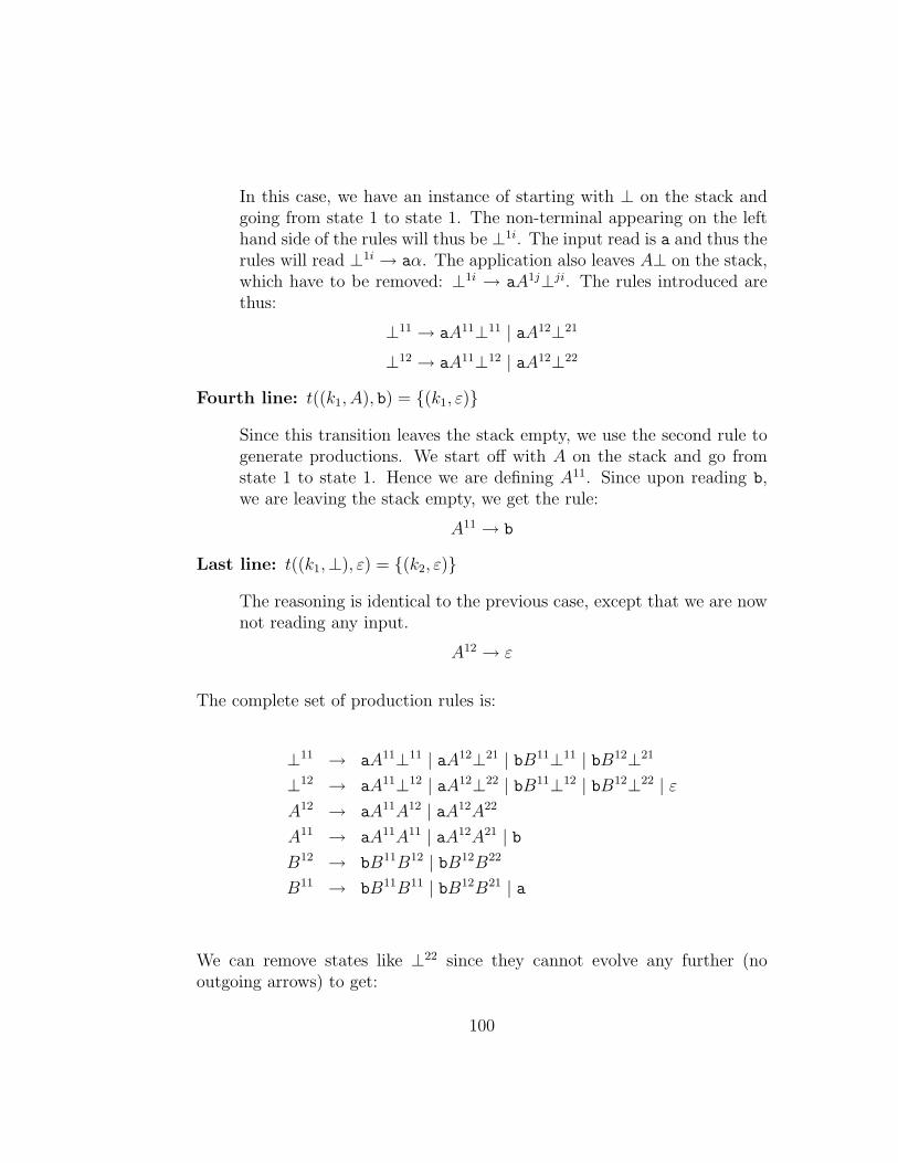
In this case, we have an instance of starting with ⊥ on the stack andgoing from state 1 to state 1. The non-terminal appearing on the lefthand side of the rules will thus be ⊥1i. The input read is a and thus therules will read ⊥1i → aα. The application also leaves A⊥ on the stack,which have to be removed: ⊥1i → aA1j⊥ji. The rules introduced arethus:

⊥11 → aA11⊥11 | aA12⊥21

⊥12 → aA11⊥12 | aA12⊥22

Fourth line: t((k1, A), b) = {(k1, ε)}

Since this transition leaves the stack empty, we use the second rule togenerate productions. We start off with A on the stack and go fromstate 1 to state 1. Hence we are defining A11. Since upon reading b,we are leaving the stack empty, we get the rule:

A11 → b

Last line: t((k1,⊥), ε) = {(k2, ε)}

The reasoning is identical to the previous case, except that we are nownot reading any input.

A12 → ε

The complete set of production rules is:

⊥11 → aA11⊥11 | aA12⊥21 | bB11⊥11 | bB12⊥21

⊥12 → aA11⊥12 | aA12⊥22 | bB11⊥12 | bB12⊥22 | εA12 → aA11A12 | aA12A22

A11 → aA11A11 | aA12A21 | bB12 → bB11B12 | bB12B22

B11 → bB11B11 | bB12B21 | a

We can remove states like ⊥22 since they cannot evolve any further (nooutgoing arrows) to get:

100

⊥11 → aA11⊥11 | bB11⊥11

⊥12 → aA11⊥12 | bB11⊥12 | εA12 → aA11A12

A11 → aA11A11 | bB12 → bB11B12

B11 → bB11B11 | a

Now we note that from the initial state ⊥12 only B11 and A11 are reachable.Copying and renaming the non-terminal symbols, we get:

S → aAS | bBS | εA → aAA | bA → bBB | a

6.5 Exercises

1. Construct an NPDA to recognize valid strings in the language describedusing the BNF notation (with initial non-terminal 〈program〉):

〈var〉 ::= a | b〈val〉 ::= 0 | 1〈skip〉 ::= I〈assign〉 ::= 〈var〉=〈var〉 | 〈var〉=〈val〉〈instr〉 ::= 〈assign〉 | 〈skip〉〈program〉 ::= 〈instr〉 | 〈instr〉;〈program〉

Expand the grammar to deal with:

• Program blocks with { and } used to begin and end blocks (re-spectively)

• Conditionals, of the form 〈program-block〉/ 〈var〉 . 〈program-block〉(P / b . Q is read ‘P if b, else Q).

101

• While loops of the form 〈var〉 ∗ 〈program-block〉.

2. Consider the NPDA depicted below:

( ,a)/

( ,a)/( ,b)/

( , )/

(b,b)/bb( ,b)/b(b,a)/

( ,b)/b1

k2 3k

k

k4

(a) Describe the language recognized by this NPDA.

(b) Calculate an equivalent NPDA with one final state.

3. Consider the following NPDA.

( , )/

( ,a)/B

(B,b)/(B,a)/BB

E

S

(a) Describe what strings it accepts.

(b) Construct a context free grammar which recognizes the same lan-guage as accepted by the automaton.

102

Chapter 7

Minimization and NormalForms

7.1 Motivation

We have seen various examples in which distinct grammars or automata pro-duce the same language. This property makes it difficult to compare gram-mars and automata without reverting back to the language they produce.Similarly, there is the issue of optimization, where, for automization reasons,we would like grammars to have as few non-terminals, and automata as fewstates as possible.

Imagine we are to discuss properties of triangles — any triangle in any posi-tion in a three dimensional space is to be studied. Clearly, we can define theset of all triangles to be the set of all 3-tuples of points referred to in cartesiannotation (x, y, z). Obviously, there are other possible ways of defining theset of all triangles, but this is the one we choose.

Now, imagine that for a particular application, we are only interested in thelength of the sides of a triangle. With this in mind, we define an equivalencerelation on triangles, and say that a triangle t1 is equivalent to a triangle t2if and only if the lengths of the sides of t1 are the same as those of t2. Notethat this will include mirror image triangles to be considered as equivalent.

The process of checking the equivalence between two triangles needs consid-erable computation. However, we notice that moving triangles around space(including rotation, translation and flipping) does not change the triangle in

103

any way (as far as our interests are concerned). We could move around anytriangle we are given such that:

1. The longest side starts at the origin and extends in the positive x-axisdirection.

2. If we call the point at the origin A, and the other point lying on thex-axis B, we flip the triangle such that AB is the second longest side,and B lies in the xy-plane.

If we call a triangle which satisfies these criteria, a normal form triangle,we notice that every triangle has an equivalent normal form triangle. Fur-thermore, for every triangle, there is only one such equivalent normal formtriangle. This allows us to compare triangles just by comparing their normalforms (now two triangles are equivalent exactly when they have a commonnormal form) and certain operations may be simpler to perform on the nor-mal form (for example, the area covered by a normal form triangle is simplyhalf the x coordinate of the second point multiplied by the y coordinate ofthe third point).

Furthermore, in certain cases, checking the equivalence of two objects maybe much more difficult than translating them into their normal forms andcomparing the results. This was not the case in the restricted trianglesexample, since rotation of a triangle is much more computationally intensivethan calculating the lengths of the sides.

This is the approach we would like to take to formal languages. If we canfind a normal form (such that every grammar/automaton has one and onlyone equivalent grammar in normal form), we can then compare the normalforms of grammars rather than general grammars (which would be easier).A normal form is sometimes called a canonical form.

We are thus addressing two different questions in this chapter:

• Can we find a normal form for grammars and automata?

• Can we find an easy algorithm to minimize grammars and automata?

104

7.2 Regular Languages

We start off by considering the simpler class of regular languages. Clearly,by the theorem stating that finite state automata and regular grammars areequally expressive, the question will be the same whether we consider eitherof the two. In this case we will be considering deterministic finite stateautomata.

7.2.1 Overview of the Solution

Look at the total DFSA depicted below:

a

b

ab

C D

a abb

b a

∆

A B

Essentially, the states are a means of defining an equivalence relationship onthe input strings. Two strings are considered equivalent (with respect to thisautomaton) if and only, when the automaton is started up with either string,in both cases, it ends up in the same state. Thus, for example, the stringsaba and ababa both send the automaton to state D and are thus related.Similarly, b and aa send the automaton from the start state to state ∆ andare similarly related.

Equivalence relations define a partition of the underlying set. Thus, equiva-lence with respect to this automaton partitions the set of all strings over a

and b into a number of parts (equal to the number of states, 5).

Clearly, we cannot define a single state automaton with the same languageas given by this automaton. Does this mean that there is a lower limit tothe number of meaningful partitions we can divide the set of all strings overan alphabet into?

It turns out that for every regular language there is such a constant. We canalso construct a total DFSA with this number of states, and furthermore, it isunique (that is, there is no other DFSA with the same number of states butdifferent connections between them which gives the same language). This

105

completes our search for a minimal automaton and a canonical form forDFSA (and hence regular languages).

The strategy of the proof is thus:

1. Define equivalence with respect to a particular DFSA.

2. Show that the number of equivalence classes (partitions) for the par-ticular language in question has a fixed lower bound.

3. Design a machine which recognizes the language in question with theminimal number of states.

4. Show that it is unique.

7.2.2 Formal Analysis

We will start by defining an equivalence relation on strings for any givenlanguage.

Definition: For a given language L over alphabet Σ, we define the relation≡L on strings over Σ:

≡L ⊆ Σ∗ × Σ∗

x ≡L ydef= ∀z : Σ∗ · xz ∈ L ⇔ yz ∈ L

Proposition: ≡L is an equivalence relation.

Example: Consider the language L = (ab)+. By definition of the ≡L, wecan show that ab ≡L abab. The proof would look like:

abx ∈ L

⇔ abx ∈ (ab)+

⇔ x ∈ (ab)∗

⇔ ababx ∈ (ab)+

⇔ ababx ∈ L

106

In fact, the set of all strings with which ab is related turns out to be the set{(ab)n|n > 0}. This is usually referred to as the equivalence class of ab for≡L, and written as [ab]≡L

.

Similarly, we can show that a ≡L aba, and that [a]≡L= (ab)∗a.

Using this kind of reasoning we end up with 4 distinct equivalent classeswhich span the whole of Σ∗. These are [ε]≡L

, [a]≡L, [ab]≡L

, [b]≡L.

Now consider the following DFSA, which we have already encountered before:

a

b

ab

C D

a abb

b a

∆

A B

Note that all the strings in the equivalence class of ab, take the automatonfrom A to C. Similarly, all strings in the equivalence class of b take it fromA to ∆ and those in the equivalence class of ε take us from A to A. However,those in the equivalence class of a, take us from A either to B or to D. Canwe construct a DFSA with the same language but where the equivalenceclasses of ≡L are intimately related to single states? The answer in this caseis positive, and we can construct the following automaton with the samelanguage:

b a

∆

a

a bb

Bb

aCA

Intuitively, it should be clear that we cannot do any better than this and aDFSA with less than 4 states should be impossible. The following theoremformalizes and generalizes the arguments presented here and proves that suchan automaton is in fact minimal and unique. This answers once and for allthe questions we have been asking since the beginning of the chapter forregular languages.

Theorem: For every DFSA M there is a unique minimal DFSA M ′ suchthat M and M ′ are equivalent.

Proof: The proof is divided into steps as already discussed in section 7.2.1.

Part 1: We start by defining an equivalence relation based on the particularDFSA in question. Let M = 〈K, T, t, k1, F 〉. We define the relation over

107

strings over alphabet T such that x ≡M y if and only if both x and ytake M from state k1 to a particular state k′:

≡M ⊆ Σ∗ × Σ∗

x ≡M ydef= t∗(k1, x) = t∗(k1, y)

It is trivial to show that ≡M has as many equivalence classes as thereare states in M (|K|).

We now try to show that there is a lower limit on this number.

Part 2: We first prove that:

x ≡M y ⇒ x ≡L y

where L is the language recognized by M (L = T (M)). The proof israther straightforward:

x ≡M y

⇒ by definition of ≡M

t∗(k1, x) = t∗(k1, y)

⇒ ∀z : T ∗ · t∗(t∗(k1, x), z) = t∗(t∗(k1, y), z)

⇒ ∀z : T ∗ · t∗(k1, xz) = t∗(k1, yz)

⇒ ∀z : T ∗ · t∗(k1, xz) ∈ F ⇔ t∗(k1, yz)

⇒ by definition of T (M)

∀z : T ∗ · xz ∈ T (M) ⇔ yz ∈ T (M)

⇒ ∀z : T ∗ · xz ∈ L ⇔ yz ∈ L

⇒ x ≡L y

Hence, it follows that for any string x, [x]≡M⊆ [x]≡L

.

This implies that no equivalence class of ≡M may overlap over two ormore equivalence classes of ≡L. Thus, the partitions created by ≡L

108

still hold when we consider those created by ≡M , except that new onesare created, as shown in the figure below.

LBoundaries set by

Boundaries set byM

This means that the number of equivalence classes of ≡M cannot besmaller than the number of equivalence classes of ≡L. But the numberof equivalence classes of ≡M is the number of states of M :

|K| ≥ |{[x]≡L| x ∈ T ∗}|

Part 3: Now that we have set a lower bound on the number of states ofM , can we construct an equivalent DFSA with this number of states?Consider the automaton M0 = 〈K ′, T, t′, k′1, F

′〉 where:

K ′ = {[x]≡L| x ∈ T ∗}

t′([x]≡L, a) = [xa]≡L

k′1 = [ε]≡L

F ′ = {[x]≡L| x ∈ L}

Does this machine also generate language L?

T (M0)

= {x | t′∗(k′1, x) ∈ F ′}= {x | t′∗([ε]≡L

, x) ∈ F ′}= {x | [x]≡L

∈ F ′}= {x | x ∈ L}= L

109

Part 4: We have thus proved that we can identify the minimum number ofstates of a DFSA which recognizes language L. Furthermore, we haveidentified one such automaton. The only thing left to prove is that itis unique.

How can we define uniqueness? Clearly, if we rename a state, thedefinitions would have changed, but without effectively changing theautomaton in any relevant way. We thus define equality modulo statenames of two automata M1 and M2 by proving that there is a mappingbetween the states of the machines such that:

• the mapping relates each state from M1 with exactly one state inM2 (and vice-versa).

• M1 in state k goes to state k′ upon input a if and only if M2 in thestate related to k can act upon input a to go to the state relatedto k′.

Assume that two DFSA M1 and M2 recognize language L, and bothhave exactly n states (where n is the number of equivalence classes of≡L).

Let M i = 〈Ki, T, ti, ki1, F

i〉.

Clearly, by the reasoning in the previous steps, every state is relatedto one equivalent class of ≡L. Each state in K1 is thus related to some[x]≡L

. Similarly states in K2.

The mapping between states is thus done via these equivalence classes.Now consider states k1 ∈ K1 and state k2 ∈ K2, where both areassociated with [x]≡L

.

Thus ti∗(ki1, x) = ki for i = 1 or 2.

Now consider an input a:

t1(k1, a)

= t1(t1∗(k11, x), a)

= t1∗(k11, xa)

110

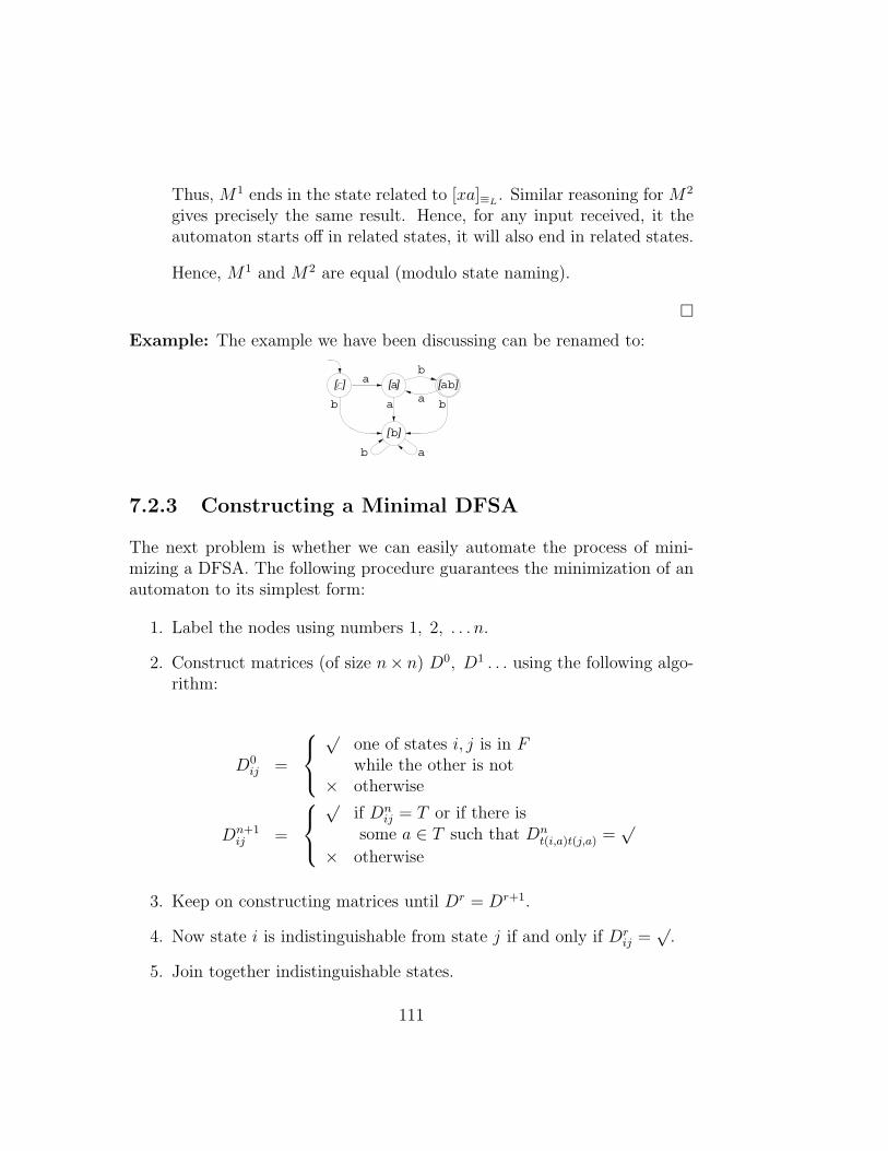
Thus, M1 ends in the state related to [xa]≡L. Similar reasoning for M2

gives precisely the same result. Hence, for any input received, it theautomaton starts off in related states, it will also end in related states.

Hence, M1 and M2 are equal (modulo state naming).

�

Example: The example we have been discussing can be renamed to:

a

a bb

b

a

b a

[ ] [ ]

b

a

[ ]

ab[ ]

7.2.3 Constructing a Minimal DFSA

The next problem is whether we can easily automate the process of mini-mizing a DFSA. The following procedure guarantees the minimization of anautomaton to its simplest form:

1. Label the nodes using numbers 1, 2, . . . n.

2. Construct matrices (of size n× n) D0, D1 . . . using the following algo-rithm:

D0ij =

√

one of states i, j is in Fwhile the other is not

× otherwise

Dn+1ij =

√

if Dnij = T or if there is

some a ∈ T such that Dnt(i,a)t(j,a) =

√

× otherwise

3. Keep on constructing matrices until Dr = Dr+1.

4. Now state i is indistinguishable from state j if and only if Drij =

√.

5. Join together indistinguishable states.

111

Note that a tick (√

) in any of the matrices Dni,j indicates that states i and j

are distinguishable (different).

Why does this algorithm work? In the first step, when creating D0, we saythat two states are different if one is terminal while the other is not. In sub-sequent steps, we say that two states are different (either if we have alreadyestablished so) or if, upon being given the same input, they evolve to stateswhich have been shown to be different. The process is better understood bygoing through an example.

Example: Look at the following example (once again!):

a

b

ab

a abb

b a

1 2 3 4

5

First of all note that for any matrix Di we construct, Dijk = Di

kj. In otherwords, the matrix will be reflected across the main diagonal. To avoid con-fusion we will only fill in the top half of the matrix.

Construction of D0: From the diagram, only state 3 is a final state. Thus allentries D0

13, D023, D0

34, D035 are true (since 3 is in F , whereas 1, 2, 4 and 5 are

not.

D0 =

× ×

√× ×

×√

× ××

√ √

× ××

Construction of D1: We start off by copying all positions already set to

√

(since they will remain so). By the definition of Dn+1, we notice that we willnow distinguish nodes one of which evolves to 3 upon an input x, whereasthe other evolves to a node which is not 3.

For example:

t(1, b) = 5

t(2, b) = 3

112

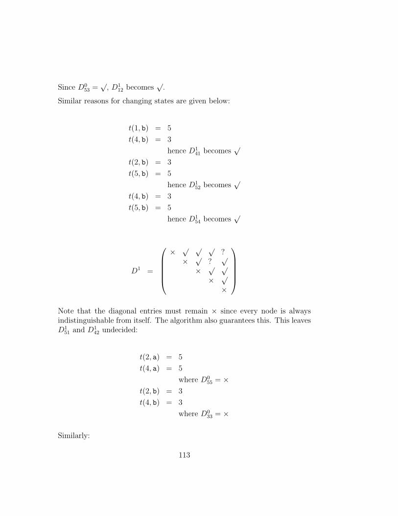
Since D053 =

√, D1

12 becomes√

.

Similar reasons for changing states are given below:

t(1, b) = 5

t(4, b) = 3

hence D141 becomes

√

t(2, b) = 3

t(5, b) = 5

hence D152 becomes

√

t(4, b) = 3

t(5, b) = 5

hence D154 becomes

√

D1 =

×

√ √ √?

×√

?√

×√ √

×√

×

Note that the diagonal entries must remain × since every node is alwaysindistinguishable from itself. The algorithm also guarantees this. This leavesD1

51 and D142 undecided:

t(2, a) = 5

t(4, a) = 5

where D055 = ×

t(2, b) = 3

t(4, b) = 3

where D033 = ×

Similarly:

113

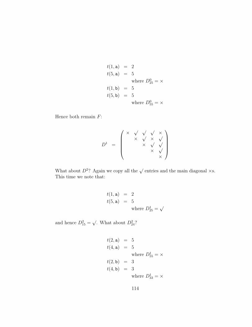
t(1, a) = 2

t(5, a) = 5

where D025 = ×

t(1, b) = 5

t(5, b) = 5

where D055 = ×

Hence both remain F :

D1 =

×

√ √ √×

×√

×√

×√ √

×√

×

What about D2? Again we copy all the

√entries and the main diagonal ×s.

This time we note that:

t(1, a) = 2

t(5, a) = 5

where D125 =

√

and hence D215 =

√. What about D2

24?

t(2, a) = 5

t(4, a) = 5

where D155 = ×

t(2, b) = 3

t(4, b) = 3

where D133 = ×

114

and hence remains ×.

D2 =

×

√ √ √ √

×√

×√

×√ √

×√

×

Calculating D3: There is now only D3

42 to consider. Again we get:

t(2, a) = 5

t(4, a) = 5

where D255 = ×

t(2, b) = 3

t(4, b) = 3

where D233 = ×

D3 thus remains exactly like D2, which allows us to stop generating matrices.

What can we conclude from D2? Apart from the main diagonal, only D224 is

×. This says that states 2 and 4 are indistinguishable and can thus be joinedinto a single state:

a

a bb

b

a

b a

1 2 3

5

7.2.4 Exercises

Consider the following regular grammar:

G = 〈Σ, N, P, S〉Σ = {a, b}N = {S, A, B}

115

P = { S → aA | bA → aBB → aA | b }

1. Obtain a total DFSA M equivalent to G.

2. Minimize automaton M to get M0.

3. Obtain a regular grammar G0 equivalent M0.

7.3 Context Free Grammars

The form for context free grammars is extremely general. A question arisesnaturally: Is there some way in which we can restrict the syntax of contextfree grammars without reducing their expressive power? The generality ofcontext free grammars usually means more difficult proofs and inefficientparsing of the language. The aim of this section is to define two normalforms for context free grammars: the Chomsky normal form and Greibachnormal form. The two different restrictions (on syntax) are aimed at differentgoals: the Chomsky normal form presents the grammar in a very restrictedmanner, making certain proofs about the language generated considerablyeasier. On the other hand, the Greibach normal form aims at producing agrammar for which the membership problem (is x ∈ L(G)?) can be efficientlyanswered.

We note that neither of these normal forms is unique. In other words, non-equality of two grammars in either of these normal forms does not guaranteethat the languages generated are different.

7.3.1 Chomsky Normal Form

Recall that productions allowed in context free grammars were of the formA → α, where A is a single non-terminal and α is a string of terminal andnon-terminal symbols.

The Chomsky normal form allows only productions from a single non-terminalto either a single terminal symbol or to a pair of non-terminal symbols.

116

Definition: A grammar G = 〈Σ, N, P, S〉 is said to be in Chomsky normalform if all the production rules in P are of the form A → α, where A ∈ Nand α ∈ Σ ∪NN .

Theorem: Any ε-free context free language L can be generated by a contextfree grammar in Chomsky normal form.

Construction: Let G = 〈Σ, N, P, S〉 by the ε-free context free grammargenerating L.

Three steps are taken to progressively discard unwanted productions:

1. We start by getting rid of productions of the form A → B, whereA, B ∈ N .

2. We then replace all rules which produce strings which include terminalsymbols (except for those which produce single terminal symbols).

3. Finally, we replace all rules which produce strings of more than twonon-terminals.

Step 1: Consider rules of the form A → B, where A, B ∈ N . We will replaceall such rules with a common left hand side collectively.

If, for a non-terminal A, there is at least one production of the form A → B,we replace all such rules by:

{A → α | ∃C ∈ N · C → α ∈ P, α /∈ N, A+⇒G C}

In practice (see example) we would consider all productions which do notgenerate a single non-terminal, and check whether the left hand side can bederived from A.

Step 2: Consider rules of the form A → α, where α contains some terminalsymbols (but α /∈ Σ). For each terminal symbol a, we replace all occurancesof a by a new non-terminal Ta, and add the rule Ta → a to compensate.

Thus, rule A → aSba would be replaced by A → TaSTbTa and the rulesTa → a and Tb → b are also added.

Step 3: Finally, we replace all rules which produce strings of (more than 2)non-terminal symbols. We replace rule A → B1B2 . . . Bn (where A, Bi ∈ Nand n > 2) with the family of rules:

117

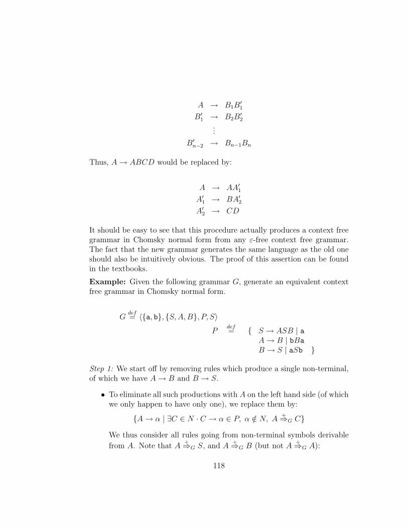
A → B1B′1

B′1 → B2B

′2

...

B′n−2 → Bn−1Bn

Thus, A → ABCD would be replaced by:

A → AA′1

A′1 → BA′

2

A′2 → CD

It should be easy to see that this procedure actually produces a context freegrammar in Chomsky normal form from any ε-free context free grammar.The fact that the new grammar generates the same language as the old oneshould also be intuitively obvious. The proof of this assertion can be foundin the textbooks.

Example: Given the following grammar G, generate an equivalent contextfree grammar in Chomsky normal form.

Gdef= 〈{a, b}, {S, A,B}, P, S〉

Pdef= { S → ASB | a

A → B | bBa

B → S | aSb }

Step 1: We start off by removing rules which produce a single non-terminal,of which we have A → B and B → S.

• To eliminate all such productions with A on the left hand side (of whichwe only happen to have only one), we replace them by:

{A → α | ∃C ∈ N · C → α ∈ P, α /∈ N, A+⇒G C}

We thus consider all rules going from non-terminal symbols derivable

from A. Note that A+⇒G S, and A

+⇒G B (but not A+⇒G A):

118

1. From A+⇒G S and the production rules from S (S → ASB and

S → a) we get:

A → ASB | a

2. Finally, from A+⇒G B and B → aSb, we get:

A → aSb

• To eliminate B → S (the only rule starting from B), we use the same

procedure as for A → B. Note that B+⇒G S (but not A or B). Hence

we only consider rules from S to get:

B → ASB | a

Thus, at the end of the first step, we have:

S → ASB | aA → ASB | a | aSb | bBa

B → ASB | a | aSb

Step 2: We now eliminate all rules producing α which includes terminalsymbols (but α /∈ Σ).

Following the procedure described earlier, we add two new non-terminal sym-bols: Ta and Tb with related rules Ta → a and Tb → b. We then replace alloccurances of a and b appearing in the rules (in the form just described)with Ta and Tb respectively.

The resultant set of production rules is now:

S → ASB | aA → ASB | a | TaSTb | TbBTa

B → ASB | a | TaSTb

Ta → a

Tb → b

119

Step 3: Finally, we remove all rules which produce more that two non-terminal symbols, by progressively adding new non-terminals:

S → AS ′ | aS ′ → SB

A → AA′ | a | TaA′′ | TbA

′′′

A′ → SB

A′′ → STb

A′′′ → BTa

B → AB′ | a | TaB′′

B′ → SB

B′′ → STb

Ta → a

Tb → b

This grammar is in Chomsky normal form.

Note that this is not unique. Clearly, we can remove redundant rules toobtain the more concise, but equivalent grammar also in Chomsky normalform:

S → AS ′ | aS ′ → SB

A → AS ′ | a | TaA′ | TbA

′′

A′ → STb

A′′ → BTa

B → AS ′ | a | TaA′

Ta → a

Tb → b

7.3.2 Greibach Normal Form

A grammar in Chomsky normal form may have a structure which makes iteasier to prove properties about. But how about implementation of a parser

120

for such a language. The new, less general form is still not very efficient toimplement. How can we hope for a better, more efficient parsing?

Recall that one of the advantages of having a regular grammar associatedwith a language was that the right hand sides of the production rules startedwith a terminal symbol, thus enabling a more efficient parse of the language.Is such a normal form possible for general context free grammars? TheGreibach normal form answers this positively. Let us start by defining exactlywhen we consider a grammar to be in Greibach normal form:

Definition: A grammar G is said to be in Greibach normal form if allthe production rules are in the form A → aα, where A ∈ N , a ∈ Σ andα ∈ (Σ ∪N)∗.

As with the Chomsky normal form, for any context free grammar, we canconstruct an equivalent one in Greibach normal form. What is the approachtaken?

First note that if any rule starts with a non-terminal, we can replace the non-terminal by the possible productions it could partake in. Thus, if A → Bαand B → β | γ, we can replace the first rule by A → βα | γα. This processcan be repeated until the rule starts with a terminal symbol. But would italways do so?

Consider A → a | Ab. Clearly, no matter how many times we replace A,we will always get a production rule starting in a non-terminal. Productionsof the form A → Aα are called left-recursive rules. We note that the rulegiven for A can generate strings a, ab, abb, etc. This can be generated byA → a | aA′ and A′ → b | bA′. This can be generalized for more complexrule sets:

If A → Aα1 | . . . | Aαn are all the left recursive productions from A, andA → β1 | . . . βm, are all the remaining productions from A, we can replacethese production rules by:

A → β1 | . . . βm | β1A′ | . . . βmA′

A′ → α1 | . . . αn | α1A′ | . . . αnA

′

where A′ is a new non-terminal symbol.

These two procedures will be used to construct the Greibach normal form ofa general ε-free, context free grammar.

121

Theorem: For any ε-free context-free language L, there is a context freegrammar in Greibach normal form which generated language L.

Construction: Let G be a context free grammar generating L. The proce-dure is then as follows:

Step 1: From G, produce an equivalent context free grammar in Chomskynormal form G′.

Step 2: Enumerate the states A1 to An, such that S is renamed to A1.

Step 3: For i starting from 1, increasing to n:

1. for any production Ai → Ajα, where i > j perform the firstprocedure. Repeat this step while possible.

2. remove any left recursive productions from Ai using the secondprocedure (and introducing A′

i).

At the end of this step, all production rules from Ai will produce astring starting either with a terminal symbol, or with a non-terminalAj such that j > i. There will also be a number of rules from A′

i whichstart off with a terminal symbol or some Aj (not A′

j).

Step 4: For i, starting from n and going down to 1, if there is some produc-tion Ai → Ajα, repeatedly perform the first procedure.

This makes sure that all production rules from Ai are in the desiredformat. Note that since all rules from A′

i cannot start from a non-terminal A′

j, we can now easily complete the desired format:

Step 5: Replace A′i → Ajα by using the first procedure.

Example: Consider the following context free grammar in Chomsky normalform:

Gdef= 〈{a, b}, {S, A,B}, P, S〉

Pdef= { S → SA | BS

A → BB | aB → AA | b }

122

To produce an equivalent grammar in Greibach normal form, we start byenumerating the non-terminals, starting with S:

G′ def= 〈{a, b}, {A1, A2, A3}, P ′, A1〉

P ′ def= { A1 → A1A2 | A3A1

A2 → A3A3 | aA3 → A2A2 | b }

We now perform step 3.

Consider i = 1. There are no productions of the form A1 → Aj, where j < 1,but there is one case of A1 → A1α. Using the second procedure to resolve it,we get:

A1 → A3A1 | A3A1A′1

A′1 → A2 | A2A

′1

When i = 2, we need to perform no changes:

A2 → A3A3 | a

Finally, for i = 3, we first perform the first procedure on A3 → A2A2,obtaining:

A3 → A3A3A2 | aA2 | b

Since no more applications of the first procedure are possible, we now turnto the second.

A3 → aA2A′3 | bA′

3 | aA2 | bA′

3 → A3A2 | A3A2A′3

Thus, at the end of step 3, we have:

123

A1 → A3A1 | A3A1A′1

A′1 → A2 | A2A

′1

A2 → A3A3 | aA3 → aA2A

′3 | bA′

3 | aA2 | bA′

3 → A3A2 | A3A2A′3

For step 4, we start with i = 3, where no modifications are necessary:

A3 → aA2A′3 | bA′

3 | aA2 | b

With i = 2 we get:

A2 → bA′3A3 | aA2A

′3A3 | a | aA2A3 | bA3

Finally, with i = 1:

A1 → aA2A′3A1 | bA′

3A1 | aA2A′3A1A

′1 | bA′

3A1A′1

Finally, we perform the first procedure on the new non-terminals A′1 and A′

3:

A′1 → bA′

3A3 | aA2A′3A3 | a | bA′

3A3A′1 | aA2A

′3A3A

′1 | aA′

1

A′3 → aA2A

′3A2 | bA′

3A2 | aA2A′3A2A

′3 | bA′

3A2A′3

The production rules in the constructed Greibach normal form grammar are:

A′1 → bA′

3A3 | aA2A′3A3 | a | bA′

3A3A′1 | aA2A

′3A3A

′1 | aA′

1

A′3 → aA2A

′3A2 | bA′

3A2 | aA2A′3A2A

′3 | bA′

3A2A′3

A1 → aA2A′3A1 | bA′

3A1 | aA2A′3A1A

′1 | bA′

3A1A′1

A2 → bA′3A3 | aA2A

′3A3 | a | aA2A3 | bA3

A3 → aA2A′3 | bA′

3 | aA2 | b

124

As with the Chomsky normal form, the Greibach normal form is not unique.For example, we can add a new non-terminal symbol X with the related rules{X → α | A1 → α} and replace some instances of A1 by X. Clearly, the twogrammars are not identical even though they are equivalent and are both inGreibach normal form.

7.3.3 Exercises

1. For the following grammar, find an equivalent Chomsky normal formgrammar:

Gdef= 〈{a, b}, {S}, P, S〉

Pdef= {S → a | b | aSa | bSb}

2. Consider the ε-free context free grammar G:

Gdef= 〈{a, b}, {S, A,B}, P, S〉

Pdef= { S → ASB | a

A → AA | aB → BB | b }

(a) Construct a grammar G′ in Chomsky normal form, such thatL(G) = L(G′).

(b) Construct a grammar G′′ in Greibach normal form, such thatL(G) = L(G′′).

3. Show that any ε-free context free grammar can be transformed into anequivalent one, where all productions are of the form A → aα, suchthat A ∈ N , a ∈ Σ and α ∈ N∗.

Produce such a grammar for the language given in question 2.

125

7.3.4 Conclusions

This section presented two possible normal forms for context free grammars.Despite not being unique normal forms, they are both useful for differentreasons.

Note that we have not proved that the transformations presented do notchange the language generated. Anybody interested in this should consultthe textbooks.

126