i

ii

FOREWORD

I am pleased to put into the hands of readers Volume-4; Issue-11: 2017 (Nov, 2017) of “International

Journal of Advanced Engineering Research and Science (IJAERS) (ISSN: 2349-6495(P)| 2456-

1908(O)” , an international journal which publishes peer reviewed quality research papers on a wide variety

of topics related to Science, Technology, Management and Humanities. Looking to the keen interest shown

by the authors and readers, the editorial board has decided to release print issue also, but this decision the

journal issue will be available in various library also in print and online version. This will motivate authors

for quick publication of their research papers. Even with these changes our objective remains the same, that

is, to encourage young researchers and academicians to think innovatively and share their research findings

with others for the betterment of mankind. This journal has DOI (Digital Object Identifier) also, this will

improve citation of research papers.

I thank all the authors of the research papers for contributing their scholarly articles. Despite many

challenges, the entire editorial board has worked tirelessly and helped me to bring out this issue of the journal

well in time. They all deserve my heartfelt thanks.

Finally, I hope the readers will make good use of this valuable research material and continue to contribute

their research finding for publication in this journal. Constructive comments and suggestions from our

readers are welcome for further improvement of the quality and usefulness of the journal.

With warm regards.

Dr. Swapnesh Taterh

Editor-in-Chief

Date: Dec, 2017

iii

Editorial/ Reviewer Board

Dr. Shuai Li Computer Science and Engineering, University of Cambridge, England, Great Britain

Behrouz Takabi Mechanical Engineering Department 3123 TAMU, College Station, TX, 77843

Dr. C.M. Singh

BE., MS(USA), PhD(USA),Post-Doctoral fellow at NASA (USA), Professor, Department of Electrical &

Electronics Engineering, INDIA

Dr. Gamal Abd El-Nasser Ahmed Mohamed Said Computer Lecturer, Department of Computer and Information Technology, Port Training Institute (PTI),

Arab Academy For Science, Technology and Maritime Transport, Egypt

Dr. Ram Karan Singh

BE.(Civil Engineering), M.Tech.(Hydraulics Engineering), PhD(Hydraulics & Water Resources

Engineering),BITS- Pilani, Professor, Department of Civil Engineering,King Khalid University, Saudi

Arabia.

Dr. Asheesh Kumar Shah

IIM Calcutta, Wharton School of Business, DAVV INDORE, SGSITS, Indore

Country Head at CrafSOL Technology Pvt.Ltd, Country Coordinator at French Embassy, Project

Coordinator at IIT Delhi, INDIA

Dr. A. Heidari Faculty of Chemistry, California South University (CSU), Irvine, California, USA

Dr. Swapnesh Taterh

Ph.d with Specialization in Information System Security, Associate Professor, Department of Computer

Science Engineering, Amity University, INDIA

Dr. Ebrahim Nohani

Ph.D.(hydraulic Structures), Department of hydraulic Structures,Islamic Azad University, Dezful, IRAN.

Dr. Dinh Tran Ngoc Huy

Specialization Banking and Finance, Professor, Department Banking and Finance, Viet Nam

Dr.Sameh El-Sayed Mohamed Yehia

Assistant Professor, Civil Engineering (Structural), Higher Institute of Engineering -El-Shorouk Academy,

Cairo, Egypt

Dr.AhmadadNabihZaki Rashed

Specialization Optical Communication System,Professor,Department of Electronic Engineering,

Menoufia University

Dr. Alok Kumar Bharadwaj

BE(AMU), ME(IIT, Roorkee), Ph.D (AMU),Professor, Department of Electrical Engineering, INDIA

Dr. M. Kannan

Specialization in Software Engineering and Data mining

Ph.D, Professor, Computer Science,SCSVMV University, Kanchipuram, India

iv

Dr. Sambit Kumar Mishra

Specialization Database Management Systems, BE, ME, Ph.D,Professor, Computer Science Engineering

Gandhi Institute for Education and Technology, Baniatangi, Khordha, India

Dr. M. Venkata Ramana

Specialization in Nano Crystal Technology

Ph. D, Professor, Physics, Andhara Pradesh, INDIA

DR. C. M. Velu

Prof.& HOD, CSE, Datta Kala Group of Institutions, Pune, India

Dr. Rabindra Kayastha

Associate Professor, Department of Natural Sciences, School of Science, Kathmandu University, Nepal

Dr. P. Suresh

Specialization in Grid Computing and Networking, Associate Professor, Department of Information

Technology, Engineering College, Erode, Tamil Nadu ,INDIA

Dr. Uma Choudhary

Specialization in Software Engineering Associate Professor, Department of Computer Science Mody

University, Lakshmangarh, India

Dr.Varun Gupta

Network Engineer,National Informatics Center , Delhi ,India

Dr. Hanuman Prasad Agrawal

Specialization in Power Systems Engineering Department of Electrical Engineering, JK Lakshmipat

University, Jaipur, India

Dr. Hou, Cheng-I

Specialization in Software Engineering, Artificial Intelligence, Wisdom Tourism, Leisure Agriculture and

Farm Planning, Associate Professor, Department of Tourism and MICE, Chung Hua University, Hsinchu

Taiwan

Dr. Anil Trimbakrao Gaikwad

Associate Professor at Bharati Vidyapeeth University, Institute of Management , Kolhapur, India

Dr. Ahmed Kadhim Hussein

Department of Mechanical Engineering, College of Engineering, University of Babylon, Republic of Iraq

Mr. T. Rajkiran Reddy

Specialization in Networing and Telecom, Research Database Specialist, Quantile Analytics, India

M. Hadi Amini

Carnegie Mellon University, USA

v

Vol-4, Issue-11, November 2017

Sr

No. Detail with DOI

1

3D Reservoir Study for Yamama Formation in Nasirya Oil field in Southern of Iraq

Author: Salman Z. Khorshid, Ghazi H. Al-Sharaa, Maha Fadel Mohammed

DOI: 10.22161/ijaers.4.11.1

Page No: 001-007

2

BER Performance of OFDM System in Rayleigh Fading Channel Using Cyclic Prefix

Author: Miss. Sneha Kumari Singh, Mr Ankit Tripathi

DOI: 10.22161/ijaers.4.11.2

Page No: 008-013

3

Interactive effect of tillage and wood ash on heavy metal content of soil, castor shoot and

seed

Author: Nweke I A, Ijearu S I, Dambaba N

DOI: 10.22161/ijaers.4.11.3

Page No: 014-027

4

Study of Mechanical Properties of Stabilized Lateritic Soil with Additives.

Author: Elijah O. Abe, Ezekiel A. Adetoro

DOI: 10.22161/ijaers.4.11.4

Page No: 028-032

5

Assessment of Performance Properties of Stabilized Lateritic Soil for Road Construction in

Ekiti State.

Author: Elijah O. Abe, Ezekiel A. Adetoro

DOI: 10.22161/ijaers.4.11.5

Page No: 033-039

6

Some aspects of Cold Deformation studies of Al-ZrB2 composites

Author: C. Venkatesh, B. Chaitanya, K S M Yadav

DOI: 10.22161/ijaers.4.11.6

Page No: 040-048

7

Study of Irrigation Water Supply Efficiency to Support the Productivity of Farmers (Case

Study at Kobisonta North Seram Central Maluku District)

Author: Hengky Jhony Soumokil, Obednego Dominggus Nara

DOI: 10.22161/ijaers.4.11.7

Page No: 049-057

8

The Air Flow Analysis of Coffee Plantation Based on Crops Planting Pattern of the

Triangular Grid and Shackle of Wheel graphs by using a Finite Volume Method

Author: Dafik, Muhammad Nurrohim, Arif Fatahillah, Moch. Avel Romanza P, Susanto

DOI: 10.22161/ijaers.4.11.8

Page No: 058-061

vi

9

Seismic Study at Subba Oil Field Applying Seismic Velocity Analysis

Author: Nawal Abed Al-Ridha, Zahraa Shakir Jassim

DOI: 10.22161/ijaers.4.11.9

Page No: 062-069

10

Peculiarities of a Colloidal Polysaccharide of Newly Isolated Iron Oxidizing Bacteria in

Armenia

Author: Levon Markosyan, Hamlet Badalyan, Arevik Vardanyan, Narine Vardanyan

DOI: 10.22161/ijaers.4.11.10

Page No: 070-076

11

Daylight Performance of Middle-rise Wide Span Building in Surabaya (Case Study: G-

building ITATS)

Author: Dian P.E. Laksmiyanti, Poppy F Nilasari

DOI: 10.22161/ijaers.4.11.11

Page No: 077-083

12

Application of Cubic Spline Interpolation to Fit the Stress-Strain Curve to SAE 1020 Steel

Author: Otávio Cardoso Duarte, Pedro Américo Almeida Magalhães Junior

DOI: 10.22161/ijaers.4.11.12

Page No: 084-086

13

Tensile Test: Comparison Experimental, Analytical and Numerical Methods

Author: Tatiana Lima Andrade, Pedro Américo Almeida Magalhães Júnior, Wagner Andrade

de Paula

DOI: 10.22161/ijaers.4.11.13

Page No: 087-090

14

Review on Exhaust Heat Recovery Systems in Diesel Engine

Author: Mohamed Shedid, Moses Sashi Kumar

DOI: 10.22161/ijaers.4.11.14

Page No: 091-097

15

Estimation of Reservoir Storage Capacity and Maximum Potential Head for Hydro-Power

Generation of Propose Gizab Reservoir, Afghanistan, Using Mass Curve Method

Author: Khan Mohammad Takal, Abdul Rahman Sorgul, Abdul Tawab Balakarzai

DOI: 10.22161/ijaers.4.11.15

Page No: 098-104

16

Pronunciation Remedy of Scientific Plants Names with Pair Exercise Using Flash card

Media at Students Plant Taxonomy Course

Author: Pujiastuti, Imam mudakir, Iis Nur Asyiah, Siti Murdiyah, Ika Lia Novenda, Vendi Eko

Susilo

DOI: 10.22161/ijaers.4.11.16

Page No: 105-110

17

The Effect Analysis of Traffic Volume, Velocity and Density in Dr.Siwabessy Salobar Road

Author: Selviana Walsen, La Mohamat Saleh

DOI: 10.22161/ijaers.4.11.17

Page No: 111-119

vii

18

Flexure and Shear Study of Deep Beams using Metakaolin Added Polypropylene Fibre

Reinforced Concrete

Author: S. Vijayabaskaran, M. Rajiv, A. Anandraj

DOI: 10.22161/ijaers.4.11.18

Page No: 120-125

19

Design and Analysis of RCA and CLA using CMOS, GDI, TG and ECRL Technology

Author: Kuldeep Singh Sekhawat, Gajendra Sujediya

DOI: 10.22161/ijaers.4.11.19

Page No: 126-129

20

Autoregressive Integrated Moving Average (ARIMA) Model for Forecasting Cryptocurrency

Exchange Rate in High Volatility Environment: A New Insight of Bitcoin Transaction

Author: Nashirah Abu Bakar, Sofian Rosbi

DOI: 10.22161/ijaers.4.11.20

Page No: 130-137

21

Design of Tuning Mechanism of PID Controller for Application in three Phase Induction

Motor Speed Control

Author: Alfred A. Idoko, Iliya. T. Thuku, S. Y. Musa, Chinda Amos

DOI: 10.22161/ijaers.4.11.21

Page No: 138-147

22

Experimental analysis of the operation of a solar adsorption refrigerator under Sahelian

climatic conditions: case of Burkina Faso

Author: Guy Christian Tubreoumya, Eloi Salmwendé Tiendrebeogo, Ousmane Coulibaly,

Issoufou Ouarma, Kayaba Haro, Charles Didace Konseibo, Alfa Oumar Dissa, Belkacem

Zeghmati

DOI: 10.22161/ijaers.4.11.22

Page No: 148-156

23

General Pattern Search Applied to the Optimization of the Shell and Tube Heat Exchanger

Author: Wagner H. Saldanha, Pedro A. A. M. Junior

DOI: 10.22161/ijaers.4.11.23

Page No: 157-159

24

Study the Dynamic Response of the Stiffened Shallow Shell Subjected to Multiple Layers of

Shock Waves

Author: Le Xuan Thuy

DOI: 10.22161/ijaers.4.11.24

Page No: 160-165

25

Theoretical investigation of series of diazafluorene-functionalized TTFs by using density

functional method

Author: Tahar Abbaz, Amel Bendjeddou, Didier Villemin

DOI: 10.22161/ijaers.4.11.25

Page No: 166-177

viii

26

Is the EM-Drive a Closed System?

Author: Carmine Cataldo

DOI: 10.22161/ijaers.4.11.26

Page No: 178-181

27

3D Seismic Study to Investigate the Structural and Stratigraphy of Mishrif Formation in

Kumiat Oil Field_Southern_Eastern Iraq

Author: Kamal K. Ali, Ghazi H. Alsharaa, Ansam H. Rasheed

DOI: 10.22161/ijaers.4.11.27

Page No: 182-187

28

Hydraulic jump on smooth and uneven bottom

Author: A. Mammadov

DOI: 10.22161/ijaers.4.11.28

Page No: 188-198

International Journal of Advanced Engineering Research and Science (IJAERS) [Vol-4, Issue-11, Nov- 2017]

https://dx.doi.org/10.22161/ijaers.4.11.1 ISSN: 2349-6495(P) | 2456-1908(O)

www.ijaers.com Page | 1

3D Reservoir Study for Yamama Formation in

Nasirya Oil field in Southern of Iraq Salman Z. Khorshid 1, Ghazi H. Al-Sharaa 2, Maha Fadel Mohammed3

1 Department of Geology, College of Science, University of Baghdad, Baghdad, Iraq.

2 Ministry of petroleum, Oil Exploration Company, Baghdad, Iraq.

Abstract— Nasriya oil field is located at the Southern

part of Iraq, this field is a giant and prolific, so it take a

special are from the Oil Exploration Company for

development purposes by using 3D seismic reflection.

The primary objective of this thesis is to obtain reservoir

properties and enhance the method of getting precise

information about subsurface reservoir characterizations

by improving the estimation of petrophysical properties

(effective porosity, P-wave, water saturation and

poisson’s ratio).

There are five wells in the study area penetrated the

required reservoirs within Yammam Formation. The

Synthetic seismogram of Nasriya wells were created to

conduct well tie with seismic data. These well tie was very

good matching with seismic section using best average

statistical wavelet. Five main horizons were picked from

the reflectors by using synthetic seismogram for wells

then converted to structural maps in depth domain by

using average velocity of five wells.

By using petrel program TWT maps have been

constructed from the picked horizons, Average velocity

maps calculated from the wells velocities survey data and

the sonic log information and Depth maps construction

was drawn using Direct time-depth conversion and the

general trend of these map was NW-SE. The model of low

frequency was created from the low frequency contents

from well data and the five main horizons were picked.

The seismic inversion technique was performed on post-

stack three dimensions (3D) seismic data in Nasriya oil

field.

Keywords— Seismic Inversion , Synthetic seismogram,

Check Shot correction, The wavelet, Synthetic trace,

Structural pictures of the picked horizons, Low

frequency model LFM (Initial model), Inversion results.

I. INTRODUCTION

Nasriya structure was discovered in 1975 through a

seismic investigations covered partially the southern part

of Iraq by (I.P.C.) groups [1].

Nasriya oil field is located in southern of Iraq within the

Dhi Qar governorate about 38 km north-west from the

Nasriya city figurer (1)

This research is dedicated to study of the Yamama

Formation and study reservoir characterization such as

(effective porosity) of Yamama Formation by using

software, specifically Hampson- Russell and petrel

programs.

Because of the good prospects of the oil in the rocks of

Cretaceous generally in Yamama Formation specially in

the Nasriya oil field and in view of the economic

importance of Yamama Formation, which is considered

as important formation that contains hydrocarbon

accumulation, this formation is of the one most important

oil production reservoirs in southern Iraq.

Fig.1: Location map of the study area [2].

II. SEISMIC INVERSION

Seismic inversion is the extracting and calculation process

of the earth’s structure (underlying geology that gave rise

to that seismic) and physical properties from some sets of

observed seismic data. The output of the seismic

inversion can be P-wave and S-wave velocities, density,

Poisson’s ratio, acoustic impedance and S-impedance

volumes [3],[4],[5]. The flow chart shown in figure (2) to

explain the main steps of the work process.

International Journal of Advanced Engineering Research and Science (IJAERS) [Vol-4, Issue-11, Nov- 2017]

https://dx.doi.org/10.22161/ijaers.4.11.1 ISSN: 2349-6495(P) | 2456-1908(O)

www.ijaers.com Page | 2

Fig. 2: Flow chart summarized the main steps of

inversion process [6].

III. THE WORK FLOW

Inversion is a process of extraction from seismic data that

utilized in the post stack and aim of to extract the acoustic

impedance volumes, this allows to compute the porosity

of fluids and water saturation, seismic inversion is used to

transform the seismic effect into acoustic log and density

log.

So the inversion helps to delete small wavelets and then

contributes the determine of reservoir properties with

better dispersion capacity of waves, and that the acoustic

impedance requires the integration of the data of the log

of the well so the inversion is a step integrated data and

the output data connects the wells and also matches the

seismic data. The process of description the reservoir

regularly using seismic data is not sufficient to simulate

the reservoir, and the field seismic data and the

processing of these data provide excellent side coverage

of the reservoir.

But seismology requires calculating the characteristics of

the bottom of the surface by sending controlled seismic

energy into the earth and watching the reflected waves at

the receiving stations. Synthetic seismogram synthetics

allows you to utilize all the well logs, geologic markers,

2D and 3D seismic, check shot data and structural

interpretations [7].

3.1 CHEC SHOT CORRECTION

This is basically true for vertical wells, small offset of the

source to the well, and little or no formation dip [8]. in

the study area all wells are vertical and check shot times

measured in these wells are vertical (one way time) OWT.

Figure (3) shows check shot correction have been applied

for one wells in study area (Ns-1), in well diagram there

are three track, the left track represent relation between

true vertical depth (TVD) and TWT which contain two

curves, input time in black color and corrected time in red

color, middle track represent drift curve and right track

represent original velocity from sonic log in black color

and corrected velocity in orange color.

Fig.3: Check shot correction for well Ns-1 in the study

area.

3.2 THE WAVELET

The wavelet is a wave pulse approximation for a seismic

source which contains many frequencies and is time

limited. By correlating reflection events across the wells,

an estimated cross-section of the geologic structure can be

interpreted [9]. Amplitude spectrum of the wavelet is

extracted by analyzing the auto-correlation process of a

set of traces over a selected time window [10]. The best

average wavelet that match the synthetic trace of the

wells of ( Ns-1,Ns-2, Ns-3, Ns-4, and Ns-5) figure (4).

International Journal of Advanced Engineering Research and Science (IJAERS) [Vol-4, Issue-11, Nov- 2017]

https://dx.doi.org/10.22161/ijaers.4.11.1 ISSN: 2349-6495(P) | 2456-1908(O)

www.ijaers.com Page | 3

Fig.4: The average statistical wavelet of wells Ns-1, 2, 3,

4, and 5.

3.3 SYNTHETIC TRACE

The synthetic trace in this study is created by convolution

process between reflectivity calculated from well data and

statistical extracted wavelet in first step, after gate proper

correlation between synthetic trace and seismic trace at

well location see the figure (5). The corrected synthetic

seismogram is displayed in seismic data through wells

Ns-1 and Ns-3 with picked main horizons in the study

area figure (6).

Figure (5): Synthetic seismogram of well Ns-1 with

statistical wavelet max. coeff. = 89%.

Fig.6: Inline section from 3D seismic data pass through

wells Ns-1 and Ns-3 with synthetic seismogram.

IV. STRUCTURAL PICTURES OF THE

PICKED HORIZONS

The studied reflectors were defined by using synthetic

seismogram for wells (Ns-1,2,3,4 and 5). These reflectors

were picked over all seismic cube and mapped to Top of

Yamama Formation (YA) , YB1, YB3, YC, and Top of

Sulaiy Formation in time domain, then converted to

structural maps in depth domain by using average

velocity of five wells.

By using petrel program, TWT maps have been

constructed from the picked horizons (Yamama)

respectively using sea level surface as a datum plane

TWT maps shows in general three enclosure domes with

a NW-SE axis in the middle of Nasriya Oil field, also

show these layers covered all study area with general dip

toward NE figure (7) and (8).

Fig.7: Show TWT map to the top of Yamama Formation

(unit YA).

International Journal of Advanced Engineering Research and Science (IJAERS) [Vol-4, Issue-11, Nov- 2017]

https://dx.doi.org/10.22161/ijaers.4.11.1 ISSN: 2349-6495(P) | 2456-1908(O)

www.ijaers.com Page | 4

Fig.8: Show TWT map to the top of Sulaiy Formation.

(Bottom Yamama Formation).

The average velocity was calculated from the wells

velocity survey data for the five previously well of

Nasirya oil field and the Sonic Log information

through which the cumulative time (TWT) was

calculated for the formation after the measurement

conversions from (Micro) Second to millisecond

and feet to meter and its compatibility with the

inverter, thus obtaining the inverter speed from the

output of the depth distribution of the configuration

on the double-measured time. The RMS was not

adopted to convert to the depths because of uneven

differences with the values of average velocity of

the wells and is so accurate that the correction

process is inaccurate

The maps shows generally a gradual increase from

the center of the domal shape to the all directions

approximately figures (9 and 10). In the Nasirya

Oilfield there is a relatively small decrease in the

velocity values.

Fig.9:Average velocity map of top of Yamama Formation.

Fig.10: Average velocity map of top of Sulaiy Formation.

Generally, depth estimation can be done wide range of

existing methods, but which can be separated into two

broad categories [11], In the current study, we have used

Direct time-depth conversion by using petrel program In

general, the depth maps revealed three major enclosure

domes where the first dome is located at the location of

the two wells (Ns-1, 3). The second dome is located near

the two wells (Ns-2, 4) and the third dome northwest of

the well (Ns-5) figure (11 and 12).

Fig.11: Shows depth map to the top of Yamama

Formation (unit YA).

International Journal of Advanced Engineering Research and Science (IJAERS) [Vol-4, Issue-11, Nov- 2017]

https://dx.doi.org/10.22161/ijaers.4.11.1 ISSN: 2349-6495(P) | 2456-1908(O)

www.ijaers.com Page | 5

Fig.12: Show depth map to the top of (Sulaiy Formation)

(Bottom of Yamama Formation).

V. CLOW FREQUENCY MODEL LFM

(INITIAL MODEL)

In amplitude seismic data, the common occurrence is the

absence of low-frequency content, that lost during

acquisition and processing of seismic data by the effect of

band limited wavelet of seismic sources and applied

band-pass filter to eliminate low-frequency ground-roll

and coherent high frequency noise [12]. Inversion of

seismic data alone leads to band-limited Acoustic

Impedance estimation [13], therefore, in seismic inversion

process, the low frequency content must be compensated

by build 3D geologic model of (AI) from well logs to

obtain absolute rather than relative (band-limited)

inverted property values [14], [15] figure (13) shows

Initial model.

Fig.13: Arbitrary line section passed through 3D volume

of low frequency model.

VI. INVERSION RESULTS

The Model Based Inversion (MBI) is a type of post stack

inversion to compute acoustic impedance from the

seismic datasets. The model based inversion technique is

also known as blocky inversion which was used in an

attempt to better define stratigraphic features and contacts

of interest. The final step of the inversion process is run

through all 3D seismic volume to create 3D acoustic

impedance between wells and cover all study area figure

(14). The final results of acoustic impedance (AI)

inversion and used four wells (Ns-1,2,3, and 5) to the

inverted seismic data and blind well (Ns-4) to quality

control inverted data as shown in figure (15). Acoustic

impedance (AI) from wells data were posted on vertical

sections passed through wells in the study area which

shows very good correlation between original and

calculated acoustic impedance (AI), in figures the low

acoustic impedance shows the good porosity and

promising areas in the oil field.

Fig.14: 3D inverted acoustic impedance volume resulted

from post stack inversion.

Fig.15: Arbitrary line from 3D all data pass through

well locations and shows matching between AI from

wells and calculated from seismic data.

The final results of acoustic impedance (AI) inversion, a

horizon slices of all units reservoir ( Yb1, Yb3, and Yc)

centered window beneath Yamama horizon has been out

of the (AI) inverted cube indicated a quality reservoir

units tend to be enhancement at the crest, NW-SE and

eastern sides of the anticline as shown in figure (16)

shows the low (AI) in the crest , NW and eastern side of

the fold, indicated high porosity. figure (17) shows the

low AI in the crest , NW-SE and eastern side of the fold,

indicated high porosity. and in figure (18) shows the low

(AI) in the crest and NW-SE side of the fold, indicated

high porosity.).

International Journal of Advanced Engineering Research and Science (IJAERS) [Vol-4, Issue-11, Nov- 2017]

https://dx.doi.org/10.22161/ijaers.4.11.1 ISSN: 2349-6495(P) | 2456-1908(O)

www.ijaers.com Page | 6

Fig.16: shows the low( AI) horizon slice of unit Yb1

Fig.17: shows (AI) horizon slice of unit Yb.

Fig.18: shows (AI) horizon slice of unit Yc in the crest

and NW-SE side of the fold.

VII. CONCLUSIONS

1- The Synthetic seismogram of Nasiriya wells were

created to conduct well tie with seismic data. These

well tie was good matching with seismic section.

2- There is a good match of the average statistical

wavelet with the synthetic seismogram of the wells of

(Ns-1, Ns-2, Ns-3, Ns-4, and Ns-5).

3- By using petrel program, TWT maps: have been

constructed from the picked horizon (tops of Yamama

and Sulaiy ). The result of study TWT maps appear in

general three enclosure domes with a NW-SE axis in

the middle of Nasriya Oil field with general dip

toward the NE.

4- Average velocity maps calculated from the wells

velocity survey data and the sonic log information.

The result of maps was generally a gradual increase

from the center of the domal shape to the all direction

approximately.

5- Depth maps construction in the current study, was

drawn using Direct time-depth conversion,

Depth maps were appeared general direction of the study

area is NW-SE, and the southwestern side is structurally

higher than the northeastern side. In general, the depth

maps revealed three major enclosure domes where the

first dome is located at two wells (Ns-1and Ns-3). The

second dome is located near the two wells (Ns-2 and Ns-

4) and the third dome was on the northwest of the well

(Ns-5).

6- The seismic inversion technique was performed on

post-stack three dimensions (3D) seismic data in Nasriya

oil field. The final results of acoustic impedance (AI)

inversion were used for four wells (Ns-1,2,3, and 5) to the

inverted seismic data and wildcat well (Ns-4) to quality

control inverted data. Horizon slices of all units reservoir

indicated a quality reservoir units tend to be enhanced at

the crest and eastern sides of the NW-SE anticline. The

result of inverted slices of Yb1,Yb3 and Yc in directional

mentioned later low acoustic impedance indicated to the

high effective porosity.

ACKNOWLEDGEMENTS

The words are racing and the phrases are crowded to

organize the thanksgiving which is only worthy of you

Praise be to God in the heavens and the earth , Praise be

to God and thank you the number of atoms of the

universe and beyond and beyond. Prayer and peace be

upon the prophet of Muhammad and his household.

I would like to express my special appreciation and thank

To my supervisor (Dr. Salman Z. Khorshid ) for all his

patience, guidance and continuous support of my MSc.

study and related research.

My best thanks to the dean of the college of science, head

of geology department, and postgraduate unit of

department tin Baghdad University. Thanks are due to all

the staff of Oil Exploration Company, and I would like to

thanks (Dr.Ghazi H. Al- Sharaa) for helping me and

providing all the facilities and information that

contributed to the completion of this research. Especially

I would like to thank the coordinator (Mr. Ammar

Ahmed) to help me and supporting me. Also I will not

forget I give my thanks and gratitude to those who were

able to consummation the march of my life from the

depths of my heart, thank you my parents ,my brother

and sister and my husband and all family .

International Journal of Advanced Engineering Research and Science (IJAERS) [Vol-4, Issue-11, Nov- 2017]

https://dx.doi.org/10.22161/ijaers.4.11.1 ISSN: 2349-6495(P) | 2456-1908(O)

www.ijaers.com Page | 7

And I thank all my colleagues in the Department of

Geology-University of Baghdad, and my friends, and my

gratitude to all who read this research.

REFERENCES

[1] O.E.C., (2007), Integrated reservoir study updating of

Nasriya field , oil exploration company, unpublished

study.

[2] Al-Ameri, T. K., (2010), Petroleum systems in Iraqi

oil field lectures presented in department of geology,

University of Baghdad, (Extended Abstract).

[3] Hampson-Russell, (1999), 2D and 3D Post-Stack

Seismic Modeling, Processing and Inversion.

[4] Hampson, D. P., Schuelke, J.S., Quirein, J.A., (2001),

Use of multiattribute transforms to predict log

properties from seismic data, Geophysics, January-

February, vol. 66, no. 1, PP. 220-236.

[5] Hampson-Russell, (2007), pre and post stack Seismic

Inversion Workshop.

[6] Al-Rahim, Ali, M. and Hashem, H., A., (2016),

Subsurface 3D Prediction Porosity Model from

Converted Seismic and Well Data Using Model

Based Inversion Technique, Iraqi Journal of Science,

Vol. 57, No.1A, pp: 136-174.

[7] Brown, A. R., (1999), Interpretation of three

dimensional seismic data, AAPG Memoir 42: AAPG,

Tulsa, SEG Investigations in Geophysics No. 9, 514

p.

[8] Geotz, J.F., Dupal, L. and Bowler, J. (1979), An

investigation into discrepancies between sonic log

and seismic check shot velocities. Journal of the

Australian Petroleum Exploration Association, 19,

131141.

[9] Liner, C., C.-F. Li, A. Gersztenkorn, and J. Smythe,

(2004), SPICE: A new general seismic attribute: 72

Annual International Meeting of the Society of

Exploration, Geophysicists Expanded Abstracts,

PP.433-436.

[10] Cariolaro, G., (2011), Unified Signal Theory,

Springer, 927 P.

[11] Etris, E. L., Crabtree, N. J. and Dewar, J., (2001),

True Depth Conversion, Canada Society of

Exploration Geophysicists, pp. 11-22.

[12] Russell, B., and Hampson, D., (2006), The old and

the new in seismic inversion, CSEG RECORDER 5.

[13] Lindseth, R.,( 1979), Synthetic sonic logs – a process

for stratigraphic interpretation: Geophysics, vol. 44,

pp. 3-36.

[14] Barclay, F., Bruun, A., Rasmussen, K. B., Alfaro, J.

C., Cooke, A., Cooke, D., Salter, D., Godfrey, R.,

Lowden, D., McHugo, S., Ozdemir, H., Pickering, S.,

Pineda, F. G., Herwanger, J., Volterrani, S.,

Murineddu, A., Rasmussen, A., and Roperts, R.,

(2008), Seismic inversion reading between lines,

Spring.

[15] Latimer, R.B., Davison, r., Van Ril, p., (2000), An

Interpreters Guide to Understanding and Working

with Seismic-Derived Acoustic Impedance Data, The

Leading Edeg, 19#3, 242 P.

International Journal of Advanced Engineering Research and Science (IJAERS) [Vol-4, Issue-11, Nov- 2017]

https://dx.doi.org/10.22161/ijaers.4.11.2 ISSN: 2349-6495(P) | 2456-1908(O)

www.ijaers.com Page | 8

BER Performance of OFDM System in Rayleigh

Fading Channel Using Cyclic Prefix Miss. Sneha Kumari Singh, Mr Ankit Tripathi

Post Graduate Student, Electronics Department, Scope College of Engineering, Bhopal, RGPV Bhopal, Madhya Pradesh, India

Assistant Professor, Electronics Department, Scope College of Engineering, Bhopal, RGPV Bhopal, Madhya Pradesh , India

Abstract— In this research paper, we will focused on the

bit error rate (BER) performance of Orthogonal-frequency

division multiplexing (OFDM) of various modulation

techniques. The Orthogonal Frequency Division

Multiplexing (OFDM) is the popular modulation technique

for the many wireless communication systems. In the

wireless system, the signal transmitted into channel bounces

off from the various surfaces resulting in the multiple

delayed versions of the transmitted signal arriving to the

receiver. The OFDM has trusted to be very effective in

mitigating adverse multi-path effects of a broadband

channel. The multiple signals are obtained due to the

diffraction and reflection of electromagnetic waves around

objects .The bit error rate (BER) performance of this type of

systems are evaluated in the additive white Gaussian noise

(AWGN) channel. The BER performance of the

transmission modes are calculated by calculating the bit

error rate (BER) versus signal to the noise ratio (SNR)

under the Additive white Gaussian noise (AWGN), channel.

Keywords—BER, UWB, SNR, AWGN, OFDM, QPSK,

BPSK, QAM, Rayleigh fading.

I. INTRODUCTION

It is very important to calculate the performance of the

wireless systems by considering the transmission

characteristics, parameters of the wireless channel and the

device structure.The Bit Error Rate Ratio (BER) is

considered to be one of the most extensively used

performance measures for wireless communication systems

and hence it has been extensively studied. In our research

paper, we proposed a novel approach to calculate the

average probability of error by using OFDM modulation

techniques and by considering an approximation of the

spatial filter.

In present time, ULTRA WIDE BAND (UWB)

communication technology is an emerging as a popular

standard for high-data-rate applications over wireless

communication networks. Due to the use of its high-

frequency bandwidth ,the UWB can achieve very high data

rates over the wireless connections of multiple system

devices at a low transmission power close to the noise

floor.Since the power level required for the UWB

transmissions is low, so UWB devices will not generate

significantly harmful interference to the other

communication standards. A major difference between

conventional radio transmissions and the UWB is that – the

conventional systems sends information by changing the

power level, frequency, and/or phase of a sinusoidal wave

whereas in the UWB transmissions information is

transmitted by generating radio energy at the specific time

intervals and covering a large bandwidth, thus enabling

pulse-position or time modulation.In the wireless channels,

several models have been introduced and investigated to

calculate SNR. Every models are a function of the distance

between the transceiver, the path loss exponent and the

channel gain. The Several probability distributed functions

are also available to model a time-variant parameter i.e.

channel gain.

It is highly believed that the OFDM results in an improved

multimedia download services requiring high data rates

communications, but this condition is significantly

controlled by inter-symbol interference (ISI) due to the

existence of the multiple paths. The Multicarrier modulation

techniques, including OFDM modulation are considered as

the most depending technique to overcome this problem

.The OFDM technique is a multi-carrier wireless

transmission technique which is being considered as an

excellent method for the high speed bi-directional wireless

communication of data.

II. OFDM TECHNIQUE

The Orthogonal frequency division multiplexing (OFDM) is

a wireless communications technique that breaks a

communications channel into a number of equally spaced

frequency bands. A sub-carrier having a portion of the user

information is sended in each band. Each sub-carrier is the

orthogonal (i.e. independent of each other) with other sub-

carrier; distinguishing OFDM from the commonly used

International Journal of Advanced Engineering Research and Science (IJAERS) [Vol-4, Issue-11, Nov- 2017]

https://dx.doi.org/10.22161/ijaers.4.11.2 ISSN: 2349-6495(P) | 2456-1908(O)

www.ijaers.com Page | 9

frequency division multiplexing (FDM) technique. The

FDM is a modulation technique that transmits multiple

signals simultaneously over a single transmission path.

TheOrthogonal frequency-division multiplexing (OFDM) is

the modulation technique for the European standards such

as the Digital Audio Broadcasting (DAB) and the Digital

Video Broadcasting (DVB) systems. The Orthogonal

frequency-division multiplexing (OFDM) is a process of

encoding digital data on the multiple carrier frequencies.

The data are transmit over parallel sub-channels with each

sub-channel modulated by the modulation scheme such as

BPSK, QPSK, QAM etc. The benefitof theOFDM is its

ability to cope with severe channel conditions compared to

a single carrier modulation scheme but still maintain the

data rates of a conventional scheme with the same

bandwidth. The Orthogonal Frequency Division

Multiplexing has become one of the main physical layer

techniques used in the modern communication systems.

Fig.1: OFDM Tones

Fig.2: Block diagram of OFDM Transmitter and Receiver

III. CHANNEL MODEL

1. AWGN Channel :When the impairedcommunication

channel are linear addition of wide band or the white noise

consisting constant spectral density over infinite period and

the amplitude is Gaussian distribution then such a channel

model is known as AWGN channel [1].

Fig.3:Gaussian distribution of white noise

The High data rate communication over the additive white

Gaussian noise channel (AWGN) is limited by the white

noise .The received signal in the interval range 0≤ t≤ T may

be given asr(t)=sm(t) + n(t)

Where n(t) represents the sample function of additive white

Gaussian noise (AWGN) process with power- spectral

density.

Fig.4: Model for received signal passed through AWGN

channel

2. Rayleigh channel model:TheRayleigh fading

environment is described by the many multipath

components, each having relatively similar signal

magnitude, and uniformly distributed phase, that means

there is no line of sight (LOS) path between transmitter and

receiver.The channel in which the signal takes various path

to reach the receiver after getting reflect from various

objects in the environment. The signal receiving at receiver

is sum of the reflected signal and the main signal. The

signal in the environmentget diffracted or reflected from the

objects like tree, building,moving vehicle etc and imposes

problem when the envelope of the ndividual signal is added

up [2].

International Journal of Advanced Engineering Research and Science (IJAERS) [Vol-4, Issue-11, Nov- 2017]

https://dx.doi.org/10.22161/ijaers.4.11.2 ISSN: 2349-6495(P) | 2456-1908(O)

www.ijaers.com Page | 10

Fig.5: Rayleigh Fading Scenario

3. Rician channel model:When the line of sight

propagation path is exist between transmitter and receiver

,then the dominant stationary signal component persists, the

fading of the channel is called as Rician channel. The white

noise which occurs because of Rician channel is explained

as Rician distribution. The Random multipath components

arriving at the receiver side comes from thedifferent angles

superimposing on a stationary signal [3].

IV. MODULATION SCHEMES

(i). Binary Phase Shift Keying (BPSK)

The PSK uses a finite number of phases; each areassigned

with a unique pattern of binary digits. Generally, each phase

encodes an equal number of the bits. Each pattern of the bits

generates the symbol that is denoted by the particular phase.

The BPSK is the simplest type of phase shift keying (PSK).

It consists of two phases which are separated by 180° and

so they can also be named as 2-PSK. It does not matter

exactly that where the constellation points are positioned,

and in the below figure they are represented on the real axis,

at 0° and 180°.

Fig.6:Constellations for BPSK

(ii) Quadrature Phase Shift Keying (QPSK)

The QPSK have four points on the constellation diagram,

and areequispaced around a circle. With four phases, QPSK

can encode the two bits per symbol, shown in the figure

with gray coding to reduce the bit error rate (BER) — some

times it misperceived as twice the BER of the BPSK. The

mathematical studies shows that QPSK can used either to

double the data rate when compared with a BPSK system

while maintaining the same bandwidth of the signal, or to

maintain the BPSK data ratebut halving the needed

bandwidth.

Fig.7: Constellation for QPSK

(iii). Quadrature amplitude modulation (QAM)

TheQAM is the modulation scheme which encode the

information into a carrier wave by varying the amplitude of

both the carrier wave and a - quadrature carrier that is 90ᵒ

out of phase with the main carrier wave in accordance with

the two input signals. It means that, the amplitude and the

phase of the carrier wave are simultaneously varied in

accordance to the information we want to transmit.The

symbol rate is one fourth of the bit rate. So this modulation

format produces a more spectrally efficient transmission. It

is more efficient than BPSK, QPSK.

Fig.8: Constellation for QAM

V. RESULTS AND ANALYSIS

The software MATLAB R2010a has been used to program

and simulate the complete environment. The various

parameters that have been initialized and various built in

functions have been used to implement the complete design

of the system.For this research work, Communication

Systems Toolbox has been used along with standard

MATLAB mathematics and graphics functions.

The various simulation parameters used in this research

work are shown in below table-

International Journal of Advanced Engineering Research and Science (IJAERS) [Vol-4, Issue-11, Nov- 2017]

https://dx.doi.org/10.22161/ijaers.4.11.2 ISSN: 2349-6495(P) | 2456-1908(O)

www.ijaers.com Page | 11

Table.1: Simulation Parameters

Parameter Value

Number of Subcarriers 512

FFT Length 512

Bandwidth 5x106

Sampling Frequency 2xBW

Cyclic Pad Length 64 bits

Modulation Technique BPSK, QPSK,

16QAM, 64 QAM

Simulation Results and Graphs

MATLAB software has been used to simulate the OFDM

scheme with different modulation schemes and the

performance is plotted in the form of Bit Error Rate (BER)

vs Signal to Noise Ratio(SNR) plots, as shown in the below

figures. The probability of error has also been computed

and plotted against the SNR. Figure 12 shows the power

spectral density plot against the sampling frequency, which

shows the orthogonality of the OFDM signals.

Fig.9: BPSK BER vs SNR curve

Fig.10: Probability of error for BPSK

Fig.11: BER vs SNR for QPSK

Fig.12: Probability of Error QPSK

Fig.13: BER vs SNR for 16-QAM

International Journal of Advanced Engineering Research and Science (IJAERS) [Vol-4, Issue-11, Nov- 2017]

https://dx.doi.org/10.22161/ijaers.4.11.2 ISSN: 2349-6495(P) | 2456-1908(O)

www.ijaers.com Page | 12

Fig.14: Probability of Error for 16 QAM

Fig.15: BER vs SNR for 64 QAM

Fig.16: Probability of Error for 16 QAM

Fig. 17: BER vs SNR plot

Fig.18: Probability vs SNR

Fig.19: PSD vs Sampling frequency

International Journal of Advanced Engineering Research and Science (IJAERS) [Vol-4, Issue-11, Nov- 2017]

https://dx.doi.org/10.22161/ijaers.4.11.2 ISSN: 2349-6495(P) | 2456-1908(O)

www.ijaers.com Page | 13

VI. CONCLUSION

In this research work, the OFDM model of Wireless

Communication is implemented and a number of

modulation schemes are used viz. BPSK,QAM,

QPSK,16PSK,etc. The various performance parameters like

BER, SNR etc. are to be evaluated. The channel used is

Rayleigh fading Channel, for this research. The research

work is intended to study and analyse the performance of

OFDM technique under various modulation schemes.

REFERENCES

[1] Nilesh Chide, ShreyasDeshmukh, Prof. P.B. Borole,

“Implementation of OFDM System using IFFT and

FFT”,International Journal ofEngineering Research

and Applications (IJERA), Vol. 3, Issue 1, pp.2009-

2014, January -February 2013

[2] Vidhya, R.Shankarkumar, “Ber Performance of

AWGN, Rayleigh and Rician Channel”, International

Journal of Advanced Research inComputer and

Communication Engineering Vol. 2, Issue 5, pp.308-

314,May 2013.

[3] V. Hindumathi, K. Rama Linga Reddy, K. Prabhakara

Rao, “Performance Analysis of OFDM by using

different Modulation Techniques”, International

Journal of Research and Development, Volume 3,

Issue 7, PP. 07-10, September 2012

[4] Mohammed S. Akhoirshida and Mustafa M. Matalgah-

-BER Performance Analysis of Interference-Limited

BPSK Cooperative Communication Systems with

Cochannel Interferencein Nakagami-m Fading

Channels, PAWR 2013, IEEE.

[5] Jun Lu, ThiangTjhung,Fumiyuki Adachi and Cheng Li

Huang, ―BER performance of OFDM-MDPSK

system in Frequency –Selective Rician Fading with

Diversity Reception,|| IEEE Trans. On Vehicular

Technology, vol. 49, no. 4, pp. 1216-1225, July 2000.

[6] Young Jae Ryu and Dong Seog Han, ―Timing phase

estimator overcoming Rayleigh Fading For OFDM

systems,‖ IEEE Proc., pp. 66- 67.

[7] M. Nakagami, ―The m-distribution—A general

formula of intensity distribution of rapid fading,‖ in

Statistical Methods in Radio Wave Propagation, W. C.

Hoffman, Ed. Elmsford, NY: Pergamon, 1960.

[8] Zheingjiu Kang, Kung Yao, Flavio Lorenzelli,

―Nakagami-m Fading Modeling in the Frequency

Domain for OFDM system analysis,‖ IEEE

Communication letters, vol. 7, no.10, pp. 484-486,

Oct.2003.

International Journal of Advanced Engineering Research and Science (IJAERS) [Vol-4, Issue-11, Nov- 2017]

https://dx.doi.org/10.22161/ijaers.4.11.3 ISSN: 2349-6495(P) | 2456-1908(O)

www.ijaers.com Page | 14

Interactive effect of tillage and wood ash on heavy

metal content of soil, castor shoot and seed Nweke I A1, Ijearu S I2, Dambaba N3

1,2Department of Soil Science Chukwuemeka Odumegwu Ojukwu University, Anambra State

3National Cereal Research Institute, Baddagi, Bida, Niger State

Abstract— Organic waste when used as soil amendment

improves the fertility status of soil and crop yield, but

unrestricted application on soil could lead to accumulation

of heavy metals to a level, toxic to plants themselves and the

animals that consumes them. Thus a field experiment was

conducted in three (3) different planting seasons using three

tillage methods (mound, ridge, flat) and four different rates

(0t/ha, 2t/ha, 4t/ha, 6t/ha) of wood ash to evaluate the effect

of tillage and wood ash on heavy metal; copper (Cu), boron

(B) and lead (Pb) content of soil and uptake by castor shoot

and seed. Data generated from the study was analyzed

using crop start version 7.2 and mean separation was done

using least significant difference (LSD0.05). The findings

from the study showed that the interactive effect of tillage

and wood ash on heavy metals content of soil, castor shoot

and seed were significant (P<0.05). The values obtained

decreased as the planting season increased, while the

amount was found to increase as the rates of wood ash

application increased. For soil heavy metal contents it was

observed that tillage methods had no effect on virtually all

the parameters assessed. The values obtained from ridge

and flat were higher when compared to the value of mound

with regard to soil and castor shoot heavy metal contents.

The result of the shoot also show that interaction of flat and

wood ash at the rates of 2t/ha, 4t/ha, and 6t/ha (Ft2, Ft4,

Ft6) show statistically similar results. The result of heavy

metal content of seed indicated that tillage method had no

effect in most of the heavy metal contents of the castor seed,

while Cu in 3rd year planting season were not significant

among the rates of wood ash applied. The interaction effect

of ridge and wood ash at the rates of 2t/ha, 4t/ha and 6t/ha

(Rd2, Rd4, Rd6) on Cu, 1st and 2nd season were statistically

similar, while the result from mound method was found to

increase the seed up take of most of the tested parameters.

The observed values of these tested parameters (Cu, B, Pb)

in wood ash amended plots in the three planting seasons

were within acceptable limits.

Keywords— Heavy metal, castor shoot, castor seed,

tillage, wood ash.

I. INTRODUCTION

Soil has been bequeathed by nature a natural medium for

waste disposal and filter to many contaminants and toxic

elements that might be harmful to crops, animals and man.

However, continuous disposal or the use of waste as soil

amendment can lead to the accumulation of the toxic metals

to a critical level where they become phototoxic to plants

and ecto-toxic to animals and man that will directly and

indirectly depend on plants for their livelihood. There are

increases in incurable diseases such as cancer; kidney

problems etc and most of these diseases are traced to our

food and water. One of the hopeless situations of pollution

of the soil with heavy metals according to Lone et al.,

(2008) and Jing et al., (2007) is that they cannot be

biologically degraded; they can only be transformed from

one oxidation state or organic complex to another.

Moolenar and Lexmond (1999) found out that lead (Pb) and

cadmium (Cd) is cumulative toxins that are indestructible

and can only be eliminated through excretion. When

accumulate in human body according to Wildlife, (2000)

they cause health hazards that include but not limited to

central nervous system, reduce intellectual capabilities and

hypertension (Stassen, 2002).

Though most of the trace elements are found naturally in

soil inform of their complexes or bound form their

accumulation in the environment are intensified by human

activities. According to the works of Okoronkwo et al.,

(2005); Jing et al., (2007) Lone et al., (2008) and

Umeoguaju (2009) mining and purification of lead, zinc and

cadmium, steel production, burning of wastes, and coal

burning, discharges from industrial effluents as well as

excessive use of fertilizers, pesticides application and use of

sewage and other organic wastes in farming operations are

man’s activities on soil that are capable of creating good

condition for heavy metals to enter and accumulate in the

soil environment.

However, from the agricultural point of view, most of the

organic wastes are applied in agricultural lands with a view

to improve the fertility status of the soil. Basically many

International Journal of Advanced Engineering Research and Science (IJAERS) [Vol-4, Issue-11, Nov- 2017]

https://dx.doi.org/10.22161/ijaers.4.11.3 ISSN: 2349-6495(P) | 2456-1908(O)

www.ijaers.com Page | 15

tropical soils like southeastern soils of Nigeria have low

organic matter content, plant nutrient deficiency resulting

from high rainfall and temperature. Consequently these

soils lack the strength and ability to sustain crop production

at optimum level, hence the need for organic waste as soil

amendment to increase soil nutrients and crop yield. The

work of Pierzynstic et al., (2002) have portrayed that lack of

effective waste management can have substantial negative

effects to plants and animals including man through the

introduction of pollutants into the soil environment. In

Nigeria, the efficiency of wood ash as well as tillage

systems in improving soil productivity and crop yield has

been documented in the works of Agbede et al., (2008),

Mbah et al., (2010), Ojeniyi et al., (2012), Omoju and

Ojeniyi, (2012), and Nwachukwu et al., (2012). However,

no attention has been given to contents of heavy metals of

wood ash as soil amendment. Thus the present study tend to

report on the uptake of selected heavy metals like Cu, B,

Pb, by castor shoot and seed and their accumulation in soil

following four different rates of wood ash application and

three tillage methods.

The work is intended to recommend an appropriate rates of

wood ash and frequency of application with appropriate

tillage method, all with a view to avoid excessive soil

accumulation and up take by castor plant, because oil from

the seed is very useful to man medically and industrially.

II. MATERIALS AND METHODS

Location of Experiment

This study was carried out in three different cropping

seasons at Teaching and Research Farm of Faculty of

Agriculture and National Resources Management Ebonyi

State University, Abakaliki. The area of the study is located

within latitude 06o191 N and Longitude 08o061 of the

southeast in the derived savannah agro-ecological zone of

Nigeria. The rainfall distribution is bimodal with wet season

from April to July and peak in June and September to

November. It has an average annual rainfall range of 1700 –

1800mm. The temperature of the area ranges from 27oC –

31oC. The relative humidity of the study area is between 60

– 80% and the soil is ultisol and classified as Typic

Haplustult by FDALR (1985).

Land preparation and Treatment Application

A land area measuring 41m x 15m (0.0615ha) was mapped

out and used for the study. The experimental site was

cleared of the natural vegetation using cutlass and the debris

removed. Tillage operation was done manually using hoe.

The tillage treatments are mound (Md), ridge (Rd) and flat

(Ft). Wood ash of different levels was spread uniformly on

the soil surface and buried in their respective plots

immediately after cultivation. The details of treatments used

are as follows:

1. Md0 – Mound without wood ash (Md0)

2. Rd0 - Ridge without wood ash (Rd0)

3. Ft0 - Flat without wood ash (Ft0)

4. Md + 2 t/ha of wood ash (Md2)

5. Md + 4 t/ha of wood ash (Md4)

6. Md + 6t/ha of wood ash (Md6)

7. Rd + 2t/ha of wood ash (Rd2)

8. Rd + 4t/ha of wood ash (Rd4)

9. Rd + 6t/ha of wood ash (Rd6)

10. Ft + 2t/ha of wood ash (Ft2)

11. Ft + 4t/ha of wood ash (Ft4)

12. Ft + 6t/ha of wood ash (Ft6)

Two castor seeds per hole were planted at a spacing of 0.9m

between rows and 0.45m within rows at a depth of 8cm.

There was basal application of NPK fertilizer to all plots

two weeks after planting. The seedlings were thinned down

to one plant per stand two weeks after germination.

Weeding was done manually with hoe at 3-weeks interval

till harvest. Harvesting was done when the capsules

containing the seed turn brown. The harvested spikes was

dried in the sun 2-3 days and then threshed to release the

seeds used for heavy metal content determination. The

shoot was also harvested for heavy metal studies. The same

procedure was repeated in the 2nd and 3rd year of the

experiment but without application of wood ash in the 3rd

year to test the residual effect.

Experimental Design

The total land area used for the study was 0.0615ha. The

experiment was laid out as split plot in a randomized

complete block design (RCBD), with 12 treatments

replicated 3 times to give a total of 36 plots each measuring

3m x 4m (12m2). A plot was separated by 0.5m alley and

each replicate was 1m apart. Four (4) rates of wood ash viz

control (0tha-1); wood ash (WA) at the rate of 2tha-1

equivalent to 2.4kg/plot, WA at 4tha-1 equivalent to

4.8kg/plot and WA at 6tha-1 equivalent to 7.2kg/plot was

used for the study. Each treatment was replicated 3 times

along with the three tillage methods (Mound, Ridge and

Flat) used for the study.

Soil Sample Collection

Auger soil samples were randomly taken from ten (10)

observational points in the experimental area at the depth of

0 – 20cm prior to planting. The auger soil samples were

mixed thoroughly to form a composite soil sample and used

for pre-planting soil analysis of which the result is shown in

Table I. Also the wood ash treatment used was analyzed for

International Journal of Advanced Engineering Research and Science (IJAERS) [Vol-4, Issue-11, Nov- 2017]

https://dx.doi.org/10.22161/ijaers.4.11.3 ISSN: 2349-6495(P) | 2456-1908(O)

www.ijaers.com Page | 16

determination of its heavy metal values, quantity and

chemical composition. The result is presented in Table 2.

At the end of each cropping season that is after crop

harvest, auger soil samples were collected from three

observational points in each plot, the soil samples were air

dried, sieved and used for the determination of soil heavy

metal content.

Laboratory Method

Heavy Metals (trace elements)

Heavy metals otherwise known as trace elements (metals)

are plant essential micro-nutrient elements but adversely

become toxic to plants and animals and indirectly to

humans in excess quantities. Hence they are inorganic

pollutant particles in soil.

Determination of Heavy Metals

The determination of heavy metals (Cu, B, and Pb) was by

using the method outlined by Miller et al., (1986).

Data Analysis

The data obtained from the study were subjected to an

analysis of variance test based on RCBD using CropStat

software version of 7.0, while statistically significant

difference among treatment means was estimated using the

least significant difference (LSD < 0.05).

III. RESULTS

Initial properties of the soil of the study site and wood

ash before the beginning of the study

The heavy metal content of the soil show medium values in

lead (Pb) and copper (Cu) and lower value in boron (B).

The order of their increase in the soil was Pb ˃ Cu ˃ B

(Table 1). The ash showed higher values in the tested heavy

metal contents, the order of their increase in the ash were

Cu ˃ B ˃ Pb (Table 2). There were high level content of

lead, copper and boron in ash visa-vies their content in soil.

Table.1: Initial soil parameters before treatment application

Test Parameter Value

Lead (Pb) 48.60 mgkg-1

Copper (Cu) 26.50 ‘’

Boron (B) 5.60 ‘’

Table.2: Chemical composition of the wood ash before application

Test Parameter Value

Lead (Pb) 52.28 mgkg-1

Copper (Cu) 148.00 ’’

Boron (B) 54.60 ’’

Effect of Tillage and Wood ash on soil heavy metals (Cu,

B, Pb mgkg-1)

The result of the effect of TM on heavy metals of the soil

studied (Cu, B and Pb) is presented in Table 3. The result

obtained showed that tillage methods had statistical

significant (P<0.05) effect in all the parameters tested.

Although non-significant differences in the values of B (1st

year), and 2nd year values of Cu, B and Pb were observed.

The result of Mound showed that the value of Cu decreased

in the 2nd year planting, but increased rapidly in the residual

year to the extent that the fractional differences in value of

the 1st and 2nd year value from 3rd year result were large

with 35.128mgkg-1 and 44.55mgkg-1 respectively. The

result of Boron (B) from Mound indicated decrease in value

as the planting year increased. There was a radical decrease

in value of B in the residual year when compared to the 1st

year result as the percentage decrease in value was 98.75%.

The result of lead (Pb) showed gradual decrease in value as

the year of planting increased. The result order was 1st year

result > 2nd year result > 3rd year result. The result of Ridge

for Cu showed an order of 3rd year result >1st year result >

2nd year result. The percentage decrease in value of Cu in

the 2nd year relative to the 3rd year planting result was

78.04%, this value showed that there was a rapid decrease

in the value of Cu in the 2nd year planting period.

International Journal of Advanced Engineering Research and Science (IJAERS) [Vol-4, Issue-11, Nov- 2017]

https://dx.doi.org/10.22161/ijaers.4.11.3 ISSN: 2349-6495(P) | 2456-1908(O)

www.ijaers.com Page | 17

Table.3: Effect of Tillage and Wood ash on Soil heavy Metals (Cu, B, Pb, mgkg-1)

Treatment 1st Year 2nd Year 3rd Year

Cu B Pb Cu B Pb Cu B Pb

Md0

Md2

Md4

Md6

4.440

17.900

28.000

56.200

96.340

204.600

136.300

94.800

157.800

48.220

76.400

240.400

4.800

8.950

16.600

38.500

116.000

147.400

108.300

106.600

7.200

58.600

109.500

246.100

7.900

96.450

95.800

46.900

0.940

1.940

2.000

1.750

24.400

85.080

95.110

95.380

Mean 26.635 133.010 130.705 17.213 119.575 105.350 61.763 1.658 74.993

Rd0

Rd2

Rd4

Rd6

9.600

12.000

84.400

65.400

37.200

248.100

158.700

266.800

10.400

88.200

54.116

116.700

2.440

18.100

9.600

42.200

98.700

144.500

113.800

122.600

8.860

56.200

148.100

202.900

11.080

88.400

116.400

114.500

0.750

2.370

7.500

17.600

113.700

79.967

94.200

129.000

Mean 42.850 177.700 67.354 18.085 119.900 104.015 82.595 7.055 104.217

Ft0

Ft2

Ft4

Ft6

3.840

5.790

24.100

60.233

140.300

133.467

204.000

142.800

8.540

170.400

46.600

10.240

2.350

3.800

9.600

32.100

96.200

100.500

156.400

240.200

5.400

206.400

124.500

235.800

6.540

14.100

33.950

48.200

0.550

2.370

2.450

8.810

33.990

63.760

46.410

96.640

Mean 18.491 155.142 58.945 11.963 148.325 143.025 25.697 3.545 60.198

LSD 0.05

TM 20.37 NS 53.88 NS NS NS 29.49 3.66 24.17

WA 15.27 51.55 65.37 4.09 34.35 56.60 30.56 3.54 28.75

TM x WA 0.70 14.09 0.14 0.23 0.44 85.27 0.19 0.28 28.11

TM= Tillage method; WA= Wood ash; Md0 = Mound without wood ash (WA); Md2 =Mound +2t/ha WA; Md4 = Mound +

4t/ha WA; Md6 = Mound + 6t/ha WA; Rd0 = Ridge without WA ; Rd2 = Ridge +2t/ha WA; Rd4 = Ridge + 4t/ha WA; Rd6 =

Ridge + 6t/ha WA; Ft0 = Flat without WA; Ft2 = Flat + 2t/ha WA; Ft4 = Flat + 4t/ha WA; Ft6 = Flat + 6t/ha WA

The results of B showed an increased value as the years of

planting increased, but the residual year result presented

drastic reduction in the value of B. The reduction in value

of B in 3rd year planting relative to 1st and 2nd year planting

were 96.03% and 94.12% respectively. Lead (Pb) for Ridge

showed a rapid increase in value as the planting year

increased, though the value of Pb in 2nd and 3rd year

planting are relatively similar as their difference in value

was merely 0.202mgkg-1. However, its decrease in value in

1st planting year was 35.37% relative to the 3rd year

planting. The result of Cu in Flat method indicated

decrease in value as planting year increased, though the

value which increased in the 3rd year planting was higher

than the 1st and 2nd year planting result. The result of B

showed reduction in value as the planting year increased

with drastic reduction in value in residual year. The result

of Pb from Flat showed rapid increase in value in the 2nd

year planting result when compared to the 1st year planting

result however, this value decreased rapidly in the 3rd year

result. When the tillage methods are compared, it showed

that for 1st planting period, the result order was Ridge >

Mound > Flat for Cu result. Boron showed an order of

Ridge > Flat > Mound and for Pb Mound > Ridge > Flat.

The same result scenario of 1st year was observed in 2nd

year result for Cu, but B had a contrary order as the values

of Mound and Ridge are the same with the highest value

observed in Flat. The 2nd year result of Pb showed highest

value in Flat, hence the order Flat > Mound >Ridge though

the value of Ridge and Mound are relatively alike as the

fractional difference in their values is 1.335mgkg-1. The

residual year result presents an order of result for Cu as

Ridge > Mound > Flat. The observed value of Cu in Flat

when compared to the other methods was relatively very

low. The result order of B showed that highest value of B

was observed in Ridge, next in rank was Flat, while the

least value was observed in Mound. The order of Pb result

was Ridge > Mound > Flat. The Ridge result showed very

much increased value when compared to value obtained

from Mound and Flat.

The changes in soil heavy metals contents following the

application of wood ash on the soil are shown in Table 3 for

the three cropping years. The soil heavy metal contents

(Cu, B and Pb) were significantly (P<0.05) different among

the rates of wood ash applied. The effect of wood ash

International Journal of Advanced Engineering Research and Science (IJAERS) [Vol-4, Issue-11, Nov- 2017]

https://dx.doi.org/10.22161/ijaers.4.11.3 ISSN: 2349-6495(P) | 2456-1908(O)

www.ijaers.com Page | 18

application on Mound, showed that the value of Cu in 1st

and 2nd year result was dependent on the quantity of ash

applied, as the value increased with attendant increase in

WA applied hence the result order for 1st and 2nd year was

Md6 > Md4 > Md2 > Md0. The 3rd year result depicts Md2

as having the highest content of Cu the next in rank was

Md4 among all the other rates. For the 3 years’ study Md0

consistently showed lowest value of Cu. The result of B

showed that Md2 recorded the highest value in 1st and 2nd

year planting, the next in rank was Md4 hence the result

order Md2 > Md4 > Md0 > Md6 (1st and 2nd year planting

result). The residual year presented a different order of

result whereby the highest of 2.0mgkg-1B was observed in

Md4 and the least value (0.94mgkg-1) was recorded in Md0

relative to other rates of WA applied. The result of Pb in 1st

year planting indicated non-dependent of values on the

quantity of ash applied. The 1st year planting showed

highest value of Pb was recorded in Md6, next in rank was

Md0 and the least value was obtained in Md2. The 2nd and

3rd year result of Pb showed that values obtained are

dependent on the quantity of ash applied, because the values

observed increased with increase in the rates of ash applied.

The result variation of 1st and 2nd year present an order of

Md6 > Md4 > Md2 > Md0 for the two cropping years, the

value recorded in Md6 and Md4 were higher compared to

the other two rates of WA. The effect of ash on Ridge

indicated that higher value of Cu was observed in Rd4

relative to other rates in 1st year planting, the next closest

value in rank was obtained in Rd6. The 2nd year result

showed Rd6 to have recorded the highest value

(42.20mgkg-1) and the least value (2.440mgkg-1) from Rd0,

while the 3rd year present an order of Rd4 > Rd6 > Rd2 >

Rd0. For the 3 years’ under study, the lowest values of Cu

were observed in Rd0s’ rate of which the lowest among

them is from 2nd year result. The result of B showed an

increased value on the rates in 1st and 2nd year planting, but

these values decreased drastically in the residual year. The

1st year result of B showed an order of Rd6 > Rd2 > Rd4 >

Rd0 and 2nd year Rd2 > Rd6 > Rd4 > Rd0. The residual

year showed dependency of value on the rates of WA

applied. An increased value was observed in Rd6, compared

to the values recorded in the other rates. The result

variation was Rd6 > Rd4 > Rd2 > Rd0. The lowest value of

Pb (10.4mgkg-1) was recorded in Rd0 and the highest from

Rd6 (116.700mgkg-1) relative to the values obtained from

the other rates in the 1st year planting. The 2nd year result

showed an increased value in the recorded value of Rd6 and

Rd4, though the result order showed Rd6 > Rd4 > Rd2 >

Rd0. The 3rd year result scenario changed as the Rd0 which

consistently recorded the lowest value of Pb in 1st and 2nd

planting turned out to record the next in rank to the highest

value that was obtained from Rd6, hence the order Rd6 >

Rd0 > Rd4 > Rd2. The effect of rates of WA on Flat for Cu

follows a particular order. The 1st, 2nd and 3rd year planting

result indicated increase in value as the rate of WA applied

increased and decreased in value as the planting year

increased especially when the 1st year and 2nd year planting

result values are compared. Therefore, the result order for

Cu 1st, 2nd and 3rd year results were Ft6 > Ft4 > Ft2 > Ft0.

The result of B showed an increased value in all the rates in

1st and 2nd year results but these values decreased rapidly in

the residual year. The 1st year result however showed Ft4 to

record the highest value, next to Ft4 in value was Ft6 and

the least value obtained in Ft2.The 2nd year and 3rd year

result showed that value of B obtained was dependent on

the quantity of ash applied, hence result order was Ft6 > Ft4

> Ft2 > Ft0. For the 3 years’ of study the lowest value of

0.55mgkg-1 B was observed in Rd0 of 3rd year planting

result. The 1st year planting result of Pb showed that very

low values were obtained in Ft0 and Ft6 compared to the

values of Ft2 and Ft4. Among these rates the highest value

of Pb was recorded in Ft2 and next in rank was Ft4. In 2nd

year planting result an increased value of Pb was observed

in all the rates except for Ft0 were very low value was

recorded compared to the values of the other rates of WA,

the result order is Ft6 > Ft2 > Ft4 > Ft0. The 3rd year result

showed decreased values relative to the values of 2nd year

result except for Ft0 that showed rapid increase in value in

the 3rd year result. The 3rd year result show a result

variation of Ft6 > Ft2 >Ft4 > Ft0.

The effect of tillage and wood ash presented in Table 3

showed significant differences among the tillage methods

and rates of WA applied. The result indicated that the

combination of tillage and WA has great effect on the

amount and quantity of soil heavy metals contents obtained.

The results also showed that the values of the soil heavy

metals (Cu, B and Pb) increased as the rates of WA applied

increased in the entire TM. Their values were observed to

be higher in the 1st and 2nd year planting and decreased in

the 3rd year planting period. The values observed in 4tha-1

(Md4, Rd4, Ft4) and 6tha-1 (Md6, Rd6, Ft6) rates of WA

and TM were relatively similar, but higher in value

compared to the values obtained from 2tha-1 (Md2, Rd2,

Ft2) and 0tha-1 (Md0, Rd0, Ft0) rates of WA. The result

equally showed that the value of Cu obtained from Mound

and Ridge in 1st and 3rd year planting results was

statistically similar. The values of these parameters

observed in Ridge and Flat for the 3 years’ study were

International Journal of Advanced Engineering Research and Science (IJAERS) [Vol-4, Issue-11, Nov- 2017]

https://dx.doi.org/10.22161/ijaers.4.11.3 ISSN: 2349-6495(P) | 2456-1908(O)

www.ijaers.com Page | 19

relatively similar and higher in value when compared to the

values of rates of WA in Mound. Significantly, higher

values of B > Pb > Cu were observed in 1st and 2nd year

planting period. However, these values decreased much at

3rd year planting period, while the value of Cu which was

relatively small in the 1st and 2nd year planting increased

sharply in the 3rd year planting, though the increase was not

greater than the value of Pb. The results obtained also attest

that the values of these heavy metals obtained from the

control soils (Md0, Rd0, Ft0) significantly were small when

compared with values obtained from the other rates of WA

applied which are the ash amended soils. The results of Cu,

B (1st year), B (2nd year) and Cu (3rd year) in 4tha-1 (Md4,

Rd4, Ft4) and 6tha-1 (Md6, Rd6, Ft6) were statistically

similar but significantly different with control plots. Also

the values of B (1st and 2nd year), and Cu, Pb (3rd year)

obtained from 2tha-1 and 4tha-1 WA respectively were

statistically similar but significantly better than the values

of control plots.

Effect of Tillage and Wood ash on the Heavy Metal

content of Shoot of Castor (Cu, B, Pb mgkg-1)

The effect of tillage methods on the heavy metal contents

(Cu, B, Pb) of castor shoot shown in the Table 4 showed

significant differences (P<0.05) among the tillage methods

studied. The result of Mound showed that for 3 years’

planting the value of Cu was observed to be highest in the

1st year planting of which decreased as the year of planting

increased. B and Pb result also show the same result

scenario of increased value in 1st year planting result with

attendant decrease in value as planting year increased and

there was a rapid decrease in value of the 3rd year result

when compared to the 1st and 2nd year values. The result of

Ridge and Flat for the three (Cu B and Pb) parameters for

the years of study showed decreased value as planting year

increased hence the order 1st >2nd >3rd year results. The 3rd

year results for the tested parameters in the two tillage

methods (Ridge and Flat) showed very sharp reduction in

value when compared to their values recorded in 1st and 2nd

year result. In comparison of the TM in 1st year planting

Mound showed higher value of Cu than the Ridge and the

least value from Flat while B showed an order of Ridge

>Mound> Flat.

Table.4: Effect of Tillage and Wood ash on the heavy metal content of Shoot of Castor (Cu, B, Pb mgkg-1)

Treatment 1st Year 2nd Year 3rd Year

Cu B Pb Cu B Pb Cu B Pb

Md0

Md2

Md4

Md6

1.010

1.320

1.060

0.650

20.250

12.650

23.950

32.050

1.030

1.170

1.830

1.430

0.060

0.370

0.110

0.700

19.300

11.700

23.000

21.100

0.080

0.220

0.880

0.480

0.000

0.018

0.011

0.016

1.150

1.270

1.250

1.080

0.017

0.055

0.028

0.034

Mean 1.260 22.225 1.365 0.310 18.775 0.415 0.011 1.188 0.034

Rd0

Rd2

Rd4

Rd6

0.980

1.120

1.370

1.260

32.350

21.850

33.950

43.650

1.280

1.200

2.110

1.230

0.030

0.170

0.420

0.310

31.400

20.900

33.000

42.700

0.930

0.250

1.160

0.280

0.012

0.035

0.030

0.028

0.950

1.250

1.510

1.350

0.022

0.031

0.028

0.033

Mean 1.183 32.950 1.455 0.233 32.000 0.505 0.026 1.265 0.029

Ft0

Ft2

Ft4

Ft6

1.030

1.090

1.100

1.150

21.750

15.450

16.010

6.040

1.150

1.060

1.070

1.130

0.080

0.140

0.150

0.200

20.800

14.500

15.060

5.090

0.200

0.110

0.120

0.180

0.013

0.011

0.016

0.019

1.750

1.500

1.680

1.640

0.016

0.011

0.024

0.040

Mean 1.093 14.813 1.103 0.143 13.863 0.153 0.015 1.643 0.023

LSD 0.05

TM 0.15 5.93 0.25 0.14 5.27 0.24 0.01 0.13 0.01

WA 0.14 9.46 0.24 0.15 9.34 0.23 0.01 0.24 0.01

TM x WA 0.04 0.17 0.08 0.10 1.04 0.03 0.003 0.10 0.003

TM= Tillage method; WA= Wood ash; Md0 = Mound

without wood ash (WA); Md2 =Mound +2t/ha WA; Md4 =

Mound + 4t/ha WA; Md6 = Mound + 6t/ha WA; Rd0 =

Ridge without WA ; Rd2 = Ridge +2t/ha WA; Rd4 = Ridge

+ 4t/ha WA; Rd6 = Ridge + 6t/ha WA; Ft0 = Flat without

WA; Ft2 = Flat + 2t/ha WA; Ft4 = Flat + 4t/ha WA; Ft6 =

Flat + 6t/ha WA

International Journal of Advanced Engineering Research and Science (IJAERS) [Vol-4, Issue-11, Nov- 2017]

https://dx.doi.org/10.22161/ijaers.4.11.3 ISSN: 2349-6495(P) | 2456-1908(O)

www.ijaers.com Page | 20

The reduction in the value of B recorded in Flat relative to

the Ridge value is of much value 55.04%. The variation in

the result of Pb indicates an order of Ridge >Mound >Flat,

the reduction in value in Flat was 24.19% relative to the

value obtained from Ridge. The 2nd year result showed Cu

to be higher in Mound of which the decreased value in

Ridge and Flat were 24.84% and 53.87% respectively.

Boron (B) showed increased value in Ridge, this value

decreased in Mound but lowest in Flat. Pb result presents an

order of Ridge > Mound > Flat. The result of the 3rd year for

Cu and B present a variation of Ridge > Flat >Mound, while

Pb present a contrary result order of Mound > Ridge >Flat.

For the 3 years’ of study the lowest value of Cu and B was

observed in Mound in the 3rd year planting, while that of Pb

was observed in Flat in 3rd year planting.

The rates of WA application showed decrease in value as

the year of planting increased in the entire TM and lowest

values were recorded in the 3rd year planting. The result

variation in Mound in 1st year for Cu, show Rd2 to be

higher in value compared to the other rates while the lowest

value of 0.65mgkg-1 Cu was recorded in Md6. B result

presented Md6 as the highest, next in rank was Md4 and

least value of 12.65mgkg-1 B was obtained in Md2. For Pb

result the highest value was observed in Md4 and its

decreased value in Md0 was 43.72%. The 2nd year result

variation for Cu, B and Pb showed a variation of Md6 >

Md4 > Md2 > Md0 (Cu), for B, Md4 >Md6 >Md0 >Md2

and Pb, Md4 >Md6> Md2> Md0. The result of Mound

showed non-presence of Cu in the shoot of castor from Md0

plots an indication that tend to suggest that Mound method

without soil amendment and continuous cultivation can

drastically reduce or remove entirely heavy metals from the

soil, thereby making it impossible for the growing plants to

pick them up. The other rates however showed increased

value of Cu. B showed an order of Md2> Md4 >Md0 >Md6

and Pb, Md2 > Md6 > Md4 >Md0. The result variation

indicated that higher value of B and Pb were observed in

Md2 respectively. The rate of ash on Ridge indicated higher

Cu content in Rd4 and the least in Rd0 compared to the

other rates. The B result indicated an increased value from

Rd2-Rd6, but the value of Rd0 was higher than the Rd2

values. For Pb higher value was recorded in Rd4 and the

next closed value was obtained in Rd0. The 2nd year result

for the three elements was of the same scenario with the 1st

year result, only that lower values were obtained in the rates

compared of their values in the 1st year result. The 3rd year

result of Cu and B showed increased value as rate of ash

applied increased, though a decreased value for the

elements were observed in Rd6 respectively, but higher than

their values in Rd0. The Flat result for Cu showed that the

value of Cu in 1st and 2nd year was dependent on the rate of

ash applied, hence result order of Ft6 > Ft4 > Ft2 > Ft0. Its

3rd year result presents a contrary order of Ft6 > Ft4 > Ft0 >

Ft2, but in the 3 years’ study higher value was shown to be

observed in Ft6 relative to other rates. The 1st year result of

B indicated an increased value in Ft0 of which its decreased

value in Ft6 was of much value 72.23% while for Pb higher

value was still observed in Ft0 and its decreased value in

Ft2 the least value was merely 7.83%. The 2nd year result

of B and Pb was in line with the result variation obtained

from the 1st year result only that lower values were obtained

compared to their values in the rates of 1st year result. The

3rd year planting present a result order of Ft0 > Ft4 > Ft6 >

Ft2 for B and Pb, Ft0 > Ft6 > Ft4 > Ft2 the two results

indicated higher values to have been obtained in Ft0 while

the values of Ft4 and Ft6 were relatively alike.

The result presented in Table 4 showed that the effect of

tillage methods and rates of wood ash (TM x WA) on the

heavy metal content of the shoot were significantly different

(P < 0.05) among the rates of WA and tillage methods

studied. The values of the tested elements (Cu, B and Pb)

decreased as the years of planting period increased. The

values obtained for these parameters (Cu, B and Pb) from

4tha-1 and 6tha-1 rates of WA among the tillage methods

were found to be relatively higher than the values obtained

from 0tha-1 and 2tha-1 rates. Continuous cultivation and

non-application of wastes can even lead to exhaustion or

non-uptake of some of these heavy metals as was found in

Cu in the third year planting. Tillage (Flat) and WA at the

rate of 2tha-1, 4tha-1 and 6tha-1 (Ft2, Ft4, Ft6) showed

statistically similar results for Pb and Cu in 1st and 2nd year

planting periods respectively. The yield values obtained in

Ridge and Flat were relatively higher than the values

obtained from Mound. The ash application also influences

changes in the values obtained for the parameters and the

trend of changes was observed to be in consistent. For

instance, the values of Cu in 1st and 2nd years planting were

found to increase as the rate of WA applied increased, while

the values of B and Pb decreased as the rates of WA

increased to 2tha-1 and then increased in 4tha-1 and

decreased again in 6tha-1 rates of WA. Also the values of

Cu, B and Pb in 3rd year planting obtained from 2tha-1, 4tha-

1 and 6tha-1 respectively were not significantly different

among the rates. The value trend for the 3 years of study

from the rates of WA applied showed B > Pb > Cu.

Effect of Tillage and Wood ash on heavy metal content

of Castor seed (Cu, B, Pb mgkg-1)

International Journal of Advanced Engineering Research and Science (IJAERS) [Vol-4, Issue-11, Nov- 2017]

https://dx.doi.org/10.22161/ijaers.4.11.3 ISSN: 2349-6495(P) | 2456-1908(O)

www.ijaers.com Page | 21

The effect of tillage methods on the heavy metal contents of

seed presented in Table 5 indicated non-significant

differences for B 1st and 2nd year planting and Pb for the 3

years of study. However, significant differences in Cu were

observed among the tillage methods for the years under

study. The result obtained from Mound method in 1st year

planting indicated that highest values of Cu, B and Pb were

observed in the 1st planting year of which decreased in

value as the planting year increased, with sharp reduction in

the 3rd year planting. The result of the parameters from

Ridge and Flat follow the same result order of Mound,

whereby the 1st year recorded the highest value and the

value decreased as planting year increased with greatest

decrease in value in the 3rd year planting. The result of B in

Ridge 1st and 2nd year planting however, are close as its

percentage decrease in 2nd year planting was relatively

small with a value of 3.17%. When the TM are compared,

Ridge method showed higher content of Cu, compared to

Flat and Mound that made least value. The reduction in Cu

content of Mound in the 1st year planting result was

observed to be 35.04% relative to the Ridge value. The

variation in B and Pb result for 1st and 2nd year planting

among the tillage methods were not much, though result

order showed Mound > Ridge > Flat. The residual (3rd) year

result showed that higher value of Cu content was obtained

in Mound with a value of 0.098mgkg-1 and the least value

0.045mgkg-1 obtained in Flat method. The result of B

presents a different order of Ridge > Mound > Flat while Pb

showed that Mound > Flat > Ridge.

The rates of WA application in Table 5 showed significant

differences (P<0.05) for the tested elements except for

residual year result of Cu. The result of its application on

Mound methods in 1st year planting indicated that highest

values of Cu, B and Pb were observed in Md2, Md4 and

Md6 respectively. For Cu the least values were obtained in

Md6 of which its percentage decreased value relative to

Md2 was 85.95%. This value showed greater reduction of

Cu value in Md6 while B showed 76.27% value reduction

in Md0 relative to Md4. Pb value showed dependence of

value on the rate of ash applied as order was Md6 > Md4 >

Md2 > Md0. It showed much reduction in value in Md0

with a value of 49.746% relative to the Md6 value. The 2nd

year planting result indicated that Md2 was higher in Cu

content compared to the other rates of WA the next in rank

was Md6 and the least value from Md0. B showed least

value in Md0 and the highest value from Md4. The value of

Pb showed dependent on the rate of ash as the result order

was Md6 > Md4 > Md2 > Md0 but greater reduction in Md0

with 96.078% relative to Md6 value. The 3rd year result

showed the Cu content to be high in Md6 the closest in rank

was the value of Md2, but the Cu value decreased in Md0

with 32.20% relative to Md6 value. The result of B showed

a result order of Md2 > Md6 > Md0 > Md4. However, the

values of Md2 and Md6 as well as Md0 and Md4 did not

vary much from the other as the fractional difference in

their values were 0.017mgkg-1 and 0.005mgkg-1

respectively. The result from Mound in the residual year

for lead (Pb) indicated non-uptake of the element by the

castor seed in Md0 and Md6 plots, but its uptake in Md2

and Md4 showed that among the two rates, much of Pb

content was observed in Md4 relative to Md2. The rate of

ash on Ridge in 1st year planting indicated that higher

content of Cu was obtained from Rd2 plots, the next in rank

was observed in Rd6 plots, but the value decreased in Rd0

plots with a value of 32.97% relative to the Rd2 plots. The

B content indicated a variation of Rd6 > Rd4 > Rd0 > Rd2

of which the percentage decrease in value of the element in

Rd2 was 45.80% relative to the plots that recorded the

highest B value. The content of Pb increased as the rate of

ash increased. Although a decreased value was observed in

Rd6 of which was higher in value than the Rd0 value the

percentage difference in value between the Rd6 and Rd0

plots was 22%. The 2nd year planting result showed a

decrease in value from the 1st year planting result. The

result of Cu in this 2nd year result showed that Rd2 and Rd6

had the same value of Cu, while there was a greater

decrease in the value of Rd0 relative to the Rd6 and Rd2

values. The value of B content in this 2nd year result still

observed the scenario of 1st year result whereby the higher

content of B was obtained from Rd6 of which is greater

than the value of Rd4 and Rd0. While the least value was

observed in Rd2 of which is 46.93% decreased compared to

the value from Rd6 plots. When compared to its 1st year

results, it means that the content of B decreased with a

value of 1.13% in 2nd year planting result. The result of Pb

showed increased value as the rate of ash applied increased

to

Rd4, but decreased in Rd6. Though the observed value of

Pb in the Rd6 was decreased, it was still higher than the

value obtained in the Rd0 plots. The residual year result for

the parameter showed sharp decrease in values obtained.

The Cu content showed much decreased value in Rd4 with

a value of 76.77% relative to the value of Cu obtained from

Rd0 plots. The result of B increased in Rd4 relative to other

rates of ash applied, the next increased value was observed

in Rd0. Pb result, however, showed a variation of Rd4 >

Rd2 > Rd0 > Rd6. The values obtained for Pb also show

that there was much decreased value in Rd6 with 60.98%

International Journal of Advanced Engineering Research and Science (IJAERS) [Vol-4, Issue-11, Nov- 2017]

https://dx.doi.org/10.22161/ijaers.4.11.3 ISSN: 2349-6495(P) | 2456-1908(O)

www.ijaers.com Page | 22

relative to the value from Rd4. The result of ash on Flat

showed higher value of Cu in Ft6 and the next in rank from

Ft2 while the least value was obtained in Ft0 from the 1st

year planting result. The B and Pb content showed a

variation result order of Ft4 > Ft2 > Ft6 > Ft0 and Ft4 > Ft6

> F2 > Ft0 respectively. The values of the tested parameters

in 2nd year planting result showed decrease in value when

compared to the 1st year result. The value of Cu showed

decreased value in Ft4 when compared to the value Ft6,

while the B content showed decreased value in Ft0 relative

to the value of Ft4. The Pb value showed higher value in

Ft6 with much decreased value in Ft0 with a value of

86.96%. The residual year result showed a greater decrease

in value of the elements when compared to the 1st and 2nd

year results. The result of Cu showed an increased value in

Ft0 though the value did not vary much from the value

obtained in Ft4 as the fractional difference in their values

was merely 0.001mgkg-1. The B content showed higher

value in Ft2 with very much decreased value in Ft4 which

was 96.66% showing greater reduction of B in Ft4 relative

to Ft2 value. While Pb result indicated decrease in value as

the rate of ash applied increased, hence the result order of

Ft0 > Ft2 > Ft4 > Ft6.

The effect of tillage methods and rates of WA application

were significant (Table 5). However, the effect of Ridge

and WA at the rates of 2tha-1 (Rd2), 4tha-1 (Rd4) and 6tha-1

(Rd6) on Cu 1st and 2nd year planting were statistically

similar. The same kind of result was observed for B in the

3rd year where the Mound and the four different rates of

WA (Md0, Md2, Md4 and Md6) were statistically similar.

Table.5: Effect of Tillage and wood ash on heavy Metal Content of Castor Seed (Cu, B, Pb mgkg-1)

Treatment 1st Year 2nd Year 3rd Year

Cu B Pb Cu B Pb Cu B Pb

Md0

Md2

Md4

Md6

1.040

1.210

1.070

0.170

11.150

24.550

46.990

39.850

0.990

1.170

1.210

1.970

0.090

0.260

0.120

0.220

10.200

23.600

46.040

38.900

0.040

0.220

0.260

1.020

0.080

0.100

0.095

0.118

0.250

0.350

0.245

0.333

0.000

0.086

0.099

0.000

Mean 1.123 30.635 1.335 0.173 29.685 0.385 0.098 0.295 0.046

Rd0

Rd2

Rd4

Rd6

0.990

1.477

1.440

1.470

27.910

21.430

30.960

39.540

1.180

1.200

1.510

1.400

0.040

0.520

0.490

0.520

26.960

20.480

30.010

38.590

0.230

0.250

0.560

0.450

0.095

0.066

0.019

0.030

0.270

0.650

0.830

0.460

0.020

0.022

0.041

0.016

Mean 1.344 29.960 1.323 0.393 29.010 0.373 0.043 0.553 0.025

Ft0

Ft2

Ft4

Ft6

1.040

1.100

1.030

1.130

13.850

32.150

40.750

27.850

1.013

1.180

1.500

1.410

0.090

0.150

0.080

0.180

12.900

31.200

39.800

26.900

0.060

0.230

0.200

0.460

0.065

0.013

0.064

0.040

0.176

0.510

0.017

0.075

0.054

0.050

0.038

0.016

Mean 1.075 28.650 1.188 0.125 27.700 0.237 0.046 0.195 0.040

LSD 0.05

TM 0.11 NS NS 0.10 NS NS 0.02 0.14 NS

WA 0.15 0.22 0.17 0.14 0.21 0.16 NS 0.20 0.02

TM x WA 0.04 0.41 0.06 0.02 0.14 0.03 0.03 0.13 0.002

Md0 = Mound without wood ash (WA); Md2 =Mound +2t/ha WA; Md4 = Mound + 4t/ha WA; Md6 = Mound + 6t/ha WA;

Rd0 = Ridge without WA ; Rd2 = Ridge +2t/ha WA; Rd4 = Ridge + 4t/ha WA; Rd6 = Ridge + 6t/ha WA; Ft0 = Flat without

WA; Ft2 = Flat + 2t/ha WA; Ft4 = Flat + 4t/ha WA; Ft6 = Flat + 6t/ha WA

It was also observed that tillage methods, especially Mound

and Non-application of organic waste like WA influence

greatly the uptake of heavy metals like Pb as can be seen

from the presented result in Table 5. From the obtained

values, it was observed that the effect of tillage and WA

increased the seed uptake of B relative to the other

elements. Though these obtained values of the heavy metals

(Cu, B and Pb) content of seed decreased as the years of

planting increased. The tillage methods increased the

uptake of B by the castor seed. Statistically similar results

were obtained from Ridge and Flat for Cu in 3rd year

planting as well as Mound and Flat for Cu in the 2nd year

International Journal of Advanced Engineering Research and Science (IJAERS) [Vol-4, Issue-11, Nov- 2017]

https://dx.doi.org/10.22161/ijaers.4.11.3 ISSN: 2349-6495(P) | 2456-1908(O)

www.ijaers.com Page | 23

and B in the 3rd year planting period. Among the tillage

methods Mound was found out to increase the uptake of

tested parameters, followed by Ridge method. The WA

application showed that the values obtained from 4tha-1 and

6tha-1 rates of WA for the parameters tested were found to

be statistically similar, but significantly different from the

control plots. Examples are Cu, B (1st and 2nd year

planting) and B (3rd year) planting periods. It was equally

observed that the values of heavy metal contents (Cu, B and

Pb) of seed in each rate of WA applied decreased as the

year of planting increased and in some cases increasing the

rates of WA application increased the uptake of these heavy

metals.

IV. DISCUSSION

Soil Heavy Metals

The result of soil heavy metals after 3 years’ of study

showed that higher values are observed in 1st and 2nd year

planting compared to the 3rd year planting values in all the

tillage methods studied. The values of these parameters

observed in the Ridge and Flat for the 3 years planting were

relatively similar and higher in value when compared to

their values obtained from Mound. The value of Cu

obtained from Mound and Ridge in 1st and 3rd year

plantings were statistically similar. The yield of these

parameters could be dependent on the soil type, climate and

drainage. Griffith et al., (1993) noted that effect of tillage

systems on yield and soil parameters are highly dependent

upon soil type, drainage and climate. The nature of the

results obtained could also be attributed to the tillage depth

and rooting depth of castor plant as tillage methods affect

the sustainable use of soil resources through its influence on

soil properties. Strudley et al., (2008) found out that tillage

depth and intensity alter soil physical and chemical

properties that affect plant growth and yield. The

management effect of tillage methods and organic waste

application on a near-soil surface is vitally important

considering the effect of soil surface on water infiltration,

nutrient conservation, trace metals distribution and erosion

control. Thus, good soil quality not only produces good

crop yield, but also maintains environmental quality and

consequently plant, animal and human health (Action and

Gregorich, 1995; Franzluebbers, 2002).

The wood ash application for the 3 years study showed that

the result of Cu, B, (1st year), B (2nd year) and Cu (3rd year)

in 4tha-1 and 6tha-1 were statistically similar but

significantly different with control plot. Also the values of

B (1st year), B (2nd year) and Cu, Pb (3rd year) obtained from

2tha-1 and 4tha-1 WA respectively were statistically similar

but significantly better than the control plots. The values of

B decreased as planting years increased and among the soil

heavy metals tested it was B that decreased most in value in

the 3rd year planting season. Heavy metals concentrations in

soils are always a guide to the potential redevelopment of

the field sites. The nature of the result obtained may have

been influenced by the pH, cation exchange, organic matter

and to some extent the available P content of the soil. The

result of the 3 years study also show that the soil heavy

metals vary with the rate of WA application. The heavy

metals obtained from 0tha-1 significantly were small when

compared with the values obtained from the other rates of

WA applied. Alloway (1996) put the normal range of Cu to

be from 2 – 250 mgkg-1, while Malcon (1991) put Cu range

to be from 2 – 100 mgkg-1 the values obtained for the

element is within the range. Anthropogenic activities such

as amendment of soils with agricultural wastes increased

soil heavy metals concentration. The following authors:

Asadu et al., (2008), Nwite et al., (2008), LASEPA (2005)

and WHO (1996) reported significant increases in these soil

heavy metals in organic waste amended soils compared to

the control plots. Lead, (Pb) in its own case, is believed to

be absorbed by the soil and is highly insoluble. The values

obtained for these heavy metals differed greatly with that of

the results of Mba et al., (2006), (2009) and (2011) which

could be associated with the type of organic waste applied,

test crop used, planting period observed and the state of

climate and precipitation at the time of study. Tillage and

WA effect showed that the values of the soil heavy metals

(Cu, B, Pb) increased as the rate of WA applied increased

irrespective of the tillage method the ash was applied. The

effect on the values were observed to be higher in the 1st

and 2nd years planting and decreased in the 3rd year planting

season. Also their values obtained from 4tha-1 and 6tha-1

irrespective of the TM the WA was applied were found to

be relatively similar, but higher in value compared to their

values obtained from 2tha-1 and 0tha-1 rate of WA. The

result obtained could be associated with the type of tillage

method, waste applied and water content and infiltration

rate of the soil. Soil water content is affected by tillage

because of changes produced in infiltration, surface run-off

and evaporation. These factors are capable of influencing

the soil heavy metal contents, as some of them can be

soluble and transformed in the soil into their carbonate or

hydroxyl content which might be of help to soil nutrient

distribution and plant growth, while in water stress situation

some of them can become insoluble and adsorbed by soil

particles. Tillage methods influenced soil water storage

International Journal of Advanced Engineering Research and Science (IJAERS) [Vol-4, Issue-11, Nov- 2017]

https://dx.doi.org/10.22161/ijaers.4.11.3 ISSN: 2349-6495(P) | 2456-1908(O)

www.ijaers.com Page | 24

more than the degree of canopy formed by the different

crop varieties, according to Fabrizzi et al., (2006).

Heavy Metal Content of Shoot of Castor

The effect of tillage methods on the heavy metal contents of

castor shoot showed significant difference at P < 0.05

among the TM studied (Table 4). The values obtained in

each of the TM decreased as the planting years increased.

Their recorded values in Ridge and Flat were relatively

higher than the values obtained from the Mound. In most of

the parameters such as Cu and Pb (3rd year) their values in

Ridge and Flat were statistically similar. The same

statistical similarity applies to the values obtained from

Mound and Ridge with regard to the values of Cu, Pb (1st

and 2nd) years planting and B, Pb in the 3rd year planting

periods. The result obtained for the parameters could be

attributed to some factors such as tillage method used,

waste applied, root development and soil aggregation. For

instance, when soil is annually cultivated, roots develop

more extensively below 10 cm than with no-till systems

while intermediate root distribution occurs with minimum

tillage system and when residues are removed, there is

greater root growth in the 15 cm soil surface (Larson,

1999). This affected the yield contents of these parameters

much on the 3rd year planting period where their values

decreased remarkably, probably due to non-application of

WA. Also, the ability of Ridge and Mound to conserve

limited soil moisture might have influenced the statistical

similarity in values of the parameters observed. Rowland

(1993) observed that the traditional system of Ridge and

Mound cultivation improve aeration for roots and facilitates

the growth and development of crops. Continuous

cultivation reduces aggregate size, because small aggregates

are less stable than large ones (Nweke and Nnabude, 2014,

2015) and soils with small aggregates are more prone to

compaction, crusting, soil erosion and reduced yield. All

these invariably may have influenced the uptake of heavy

metals by the castor plant.

The trend of change in these parameters was observed to be

inconsistent irrespective of the TM. For example the values

of Cu in 1st and 2nd years planting were found to increase as

the rates of WA applied increased. While the values of B

and Pb decreased as the rates of WA increased to 2tha-1 and

then increased in 4tha-1 and decreased again in 6tha-1 rates

of WA. The value of the parameters Cu, Pb and B are

within the tolerable limits and, therefore, may not cause

toxicity problems to the crop nor cause any injury to

humans. Comparison of the rates of WA on TM indicated

that the rates of WA on Ridge show relatively higher values

in these parameters compared to Mound and Flat values.

Though the tested parameters are within the tolerable range,

they have the potential to build up rapidly to critical levels

in the soil due to continuous application of wastes in the

soil. Increasing the heavy metal contents of soil may not

only be deleterious to soil productivity but harmful to

humans and animals that invariably will depend on soil for

their livelihood. Thus, Naidu et al., (1997) stressed that

continuous application of organic waste amendment were

the greatest threat to the environment as a result of surface

input to soil system of heavy metals.

The values obtained for the parameters (Cu, B, Pb) from

4tha-1 and 6tha-1 rates WA among the tillage methods were

found to be relatively higher than the values obtained from

0tha-1 and 2tha-1 rates. Continuous cultivation and non-

application of wastes can even lead to exhaustion or non-

uptake of some of these heavy metals as was found in Cu in

the 3rd year planting. The effect of tillage (Flat) and WA at

the rate of 2tha-1, 4tha-1 and 6tha-1 showed statistically

similar results for Pb and Cu in 1st and 2nd year planting

periods respectively. Soil disturbance and subsequent

changes in soil organic matter strongly affect the stability of

soil aggregates and other soil properties (Boivin et al.,

2001; Nweke, 2015). These changes in turn will have

feedback effect on the uptake ability of the heavy metals by

the castor plant.

Heavy Metal contents of Seed

Statistically similar results were obtained from Ridge and

Flat for Cu in 3rd year planting as well as Mound and Flat

for Cu in the 2nd year and B in 3rd year planting result.

Among the TM, Mound was found out to increase the

uptake of most of the tested parameters followed by the

Ridge method and the least is Flat. Tillage is an integral part

of the crop production system that influences plant nutrients

and heavy metal uptake by plants. According to Arshad et

al., (1999), tillage is crucial for optimising productivity by

alleviating physico-chemical and biological constraints of

soil. Hence, nature of the result obtained from the three

tillage methods collaborated with the findings of Dick et al.,

(1991) and Okpoku et al., (1997) who postulated that yield

reduction have often been observed in no-tillage compared

to other methods, especially when used in poorly drained

fine textured soils. Also, it should be noted that crop

responses to tillage methods depend upon the number of

years a tillage system has been established, amendment

used and the history of the field.

The values obtained from 4tha-1 (Md4, Rd4, and Ft6) and

6tha-1 (Md6, Rd6, Ft6) rates were found to be statistically

similar but significantly different from the control plots.

Heavy metal contents of seed in each rate of WA applied

International Journal of Advanced Engineering Research and Science (IJAERS) [Vol-4, Issue-11, Nov- 2017]

https://dx.doi.org/10.22161/ijaers.4.11.3 ISSN: 2349-6495(P) | 2456-1908(O)

www.ijaers.com Page | 25

decreased as the year of planting increased. The observed

remarkable decrease in the uptake of these heavy metals in

third year planting by the castor seed could be due to non-

application of WA, which tend to portray that organic waste

application on agricultural soils can be one of the common

sources of soil contamination as the crops source out the

nutrients from the soil. Thus, Jones et al., (1991) reported

that heavy metals were absorbed at particle surface, bound

to carbonates or occluded in iron or manganese hydroxides,

organic matter and sulphide. The value of rates of WA on

Mound was observed to be relatively higher compared to

the values of rate of WA on Ridge and Flat.

From the obtained values it was equally observed that the

combined effect of tillage methods and rates of WA

increased the uptake of heavy metal like B. The observed

variations in the tested parameters among the tillage

methods and rates of WA and the three years of study

collaborated with the findings of Vousta and Samara (1996)

who reported that harvested crops show large variations in

heavy metal concentration from year to year in the same

field. This they attributed to plant uptake, variable emission

rates, deposition process and atmospheric transport. The

values obtained from Pb uptake by castor seed is in line

with the findings of Miller and Miller (2000) who observed

that Pb is not taken by plants to any degree. This

observation particularly with the present study can equally

be associated with the result of Cu.

V. CONCLUSION

Results of the study show that tillage methods and rates of

wood ash application as soil amendments increase the

heavy metal contents of soil, castor shoot and seed to non-

toxic level, the values of heavy metal increased as the rates

of wood ash increased and decreased as the planting seasons

increased. The values obtained from Ridge and Flat were

higher than the values obtained from Mound method though

Mound method was found to increase the uptake of heavy

metal contents of seed. Based on the results of the study the

use of wood ash as soil amendment on continuous basis

especially at higher rates should not exceed three

consecutive years on the same piece of land in order not to

constitute pollution problems at the near future.

REFERENCES

[1] Action, D.F. and Gregorich, L.J. (1995). The health of

our soils: Toward sustainable agriculture in Canada,

Agriculture and Agricultural food, Canada, CDR, 960

Carlingn.

[2] Agbede, F.M., Ojeniyi, S.O. and Awodun, M.M

2008). Effect of tillage methods on growth grain

yield. Northeastern Thailand J. 34:197-200.

[3] Alloway, B.J. (1996). Heavy metals in soil. Halsted

Press, John Wiley and Sons Inc. London, pp. 230 –

239.

[4] Arshad, M.A., Franzuebbers, A.J. and Azooz, R.H.

(1999). Components of surface soil structure under

conventional and no-tillage in North Western Canada.

Soil Till. Res. 53:41 – 47.

[5] Asadu, C.L.A., Ucheonye Oliobi, C. and Agada, C.

(2008). Assessment of sewage application in south-

western Nigeria. part I, impact on selected soil

morphological and physical properties. Outlook on

Agriculture, 37(1):57 – 62.

[6] Awodun M.A. (2007). Effect of saw dust ash on soil

chemical properties and cowpea performance in south

western Nigeria IJSC 2(1): 78-81.

[7] Boivin, H.B., Bummer; G. W. Horn, R; Randeler,

E., Kogel Knabner, I.; Kretschmar, R.; Stabr, K. and

Wike, B.M. (2009). Lehrbuch der Bodekunde.

Spektrum, 500pp.

[8] Dick, W.A., McCoy, E.L., Edwards, W.M. and Lal,

R. (1991). Continuous application of no-tillage to

Ohio soils. Agron. J. 83:65-73.

[9] Fabrizzi, K.P., Garcia, F.O., Costa, J.I. and Picone,

L.I. (2006). Soil water dynamics, physical properties

and corn and wheat responses to minimum and no-

tillage systems in the southern pampas of Argentina,

soil and Tillage Research, 81:57 – 69.

[10] Federal Department of Agriculture and land Resources

(1985). Reconnaissance soil survey of Anambra State

of Nigeria soil report 1985, Federal department of

Agriculture and Land Resources Lagos Nigeria.

[11] Franzluebbers, A.J. (2002). Soil organic matter

stratification ratio as an indicator of soil quality, Soil

and Tillage research 66:95 – 106.

[12] Gallardo-Lara, F., Robles, J., Esteban, E., Azeon, M.

and Nogales, R. (1984). Poder fertilizant de un

compost de fey Zn: In proceeding of J. Congreso

Nacional de la Ciencia del silo. Vol. I, SECs, Madrid,

393 – 403.

[13] Griffith, D.R., Mannering, J.V., Galloway, H.M.,

Parson, S.D. and Richey, C.B. (1993). Effect of eight

tillage planting systems on soil temperature, percent

stand, plant growth and yield of corn on five Indiana

soils Agron. J. 65:321 – 326.

[14] Islam, E.U., Yang, X., HE, Z and Mahmood, Q.

(2007). Assessing potential dietary toxicity of heavy

International Journal of Advanced Engineering Research and Science (IJAERS) [Vol-4, Issue-11, Nov- 2017]

https://dx.doi.org/10.22161/ijaers.4.11.3 ISSN: 2349-6495(P) | 2456-1908(O)

www.ijaers.com Page | 26

metals in selected vegetables and food crops, J.

Zhejiang Univ. Sci. B. 8:1-13.

[15] Jing, Y. He, Z., and Yang, X. (2007). Role of soil

rhizobacteria in phytoremediation of heavy metal

contaminated soils. J Zhejiang Univ. Sci. B. 8, 192-

207.

[16] Jones, A.S., Suter, H.G.W. and Hull, R.N. (1991).

Toxicological benchmark for screening potential

contaminants of concern for effects on sediment-

Associated Biota. Oak Ridge National Laboratory,

Tenn.

[17] Kos, B., Greman, H. and Lestan, D. (2003). Phyto-

extraction of lead, zinc and cadmium from soil by

selected plants. Plant Soil Environ. 49:548 – 563.

[18] Lagos State Environmental Protection Agency

(LASEPA) (2005). Lagos State Environmental Report

3:28 – 33.

[19] Lal, R. (1993). Soil erosion and conservation in

West Africa, P.7 -26. In D. Pimentel (ed), world soil

erosion and conservation. Int union for conservation

of nature and natural resources, Switzerland

[20] Larson, W.E. (1999). Soil Parameters for evaluating

tillage needs and operations, Soil and water

management and conservation. Soil Science and

Society Proceedings, 118-122

[21] Lone, M. I. He, Z., Stoffela, P. J. and Yang, X. (2008).

Phytoremediation of heavy metal polluted soils and

water, progress and perspectives. J. Zhejiang Univ.

Sci. B. 9, 210-220.

[22] Malcon, E.S. (1999). Bioavailability of nutrients: In

Handbook of Soil Science, CRC Press Boca Raton NY

Washington DC, pp. 73.

[23] Mbah, C.N., Idike, F.I. and Njoku, C. (2011).

Accumulation of pollutants in an ultisol amended with

burnt and unburnt rice mill wastes. J. Agric. Bul. Sci.

2(2):043 – 047.

[24] Mbah, C.N., Nwite .J.N., Njoku, C. and Nweke, I.A.

(2010). Response of maize (Zea mays l.) to different

rates of wood ash Application in acid ultisol in south

east Nigeria. Afri. J. Agric. Res. 5(7) pp 580-583.

[25] Mbah, C.N., Nwite, J.N., Ogbodo, E.N., Okonkwo,

C.I., Mbagwu, J.S.C. and Anikwe, M.A.N. (2006).

Trace elements in maize (zea mays) as influenced by

incorporation of animal wastes in dystric leptosol in

south-eastern Nigeria. J.Sci. Agric. Food Tech.

Environ. 6:33 – 39.

[26] Mbah, C.N., Orji, A. and Nweke, I.A. (2009). Effect

of organic inputs on soil properties of heavy metal

content and maize root yield on engine oil polluted

soil. J. Agric. Rural. Dev. 11(2):94 – 99.

[27] Miller, D.M. and Miller, W.P. (2000). Land

application of wastes, In: Summer M.E. (eds).

Handbook of Soil Science CRC Books New York.

[28] Moolenar, S. W and Lexmond, T. M. (1999). General

aspect of cadmium, copper, zinc and lead balance

studies in agro-ecosystems. Heavy metal balances, part

1 J Indust. Ecol. 2: 4-8.

[29] Naidu, R., Kookana, R.S., Summer, M.E., Harter,

K.D. and Tiller, K.G. (1997). Calcium sorption and

transport in variation change in soils. A review. J.

Environ. Qual. 26:608 – 617.

[30] Nwachukwu, O. I., Nyong, A. E. and Opara, U. D.

(2012) . Effect of manures on soil properties, yield and

nutrient uptake in an ultisol of southeast, Nigeria, Nig.

J. Soil Sci. 22(2):70-78.

[31] Nweke, I. A. (2015). Effect of land use on organic

matter concentration of aggregate fractions of

fallow and cultivated soils. Indian J. Appl. Res.

5(3): 507- 511.

[32] Nweke, I. A., and Nnabude, P. C. (2014). Organic

C, TN, and available P concentration in aggregate

fraction of four soils under two land use systems. J.

Res. Appl. Nat. Soci. Sci. 2(5): 273-288.

[33] Nweke, I. A., and Nnabude, P. C. (2015).

Aggregates stability of four soils as evaluated by

different indices. J. Expt. Biol. Agric. Sci. 3(3):

246-252.

[34] Nwite, J.N., Ekpe, I.I. and Ibeh, L.M. (2008).

Assessment of selected heavy metals in spent lubricant

oil contaminated and uncontaminated soil amended

with organic wastes in Abakaliki: In Proceedings of

42nd Annual Conference, Agricultural Society of

Nigeria (ASN), October 19th – 22nd 2000, Ebonyi

State University, Abakaliki, Nigeria, 556 pp.

[35] Ojeniyi, S. O. Adekiya, A. O. and Amusan, O. A.

(2012). Three year influence of tillage and poultry

manure on soil physical properties and yield of

cocoyam, Nig. J. Soil Sci. 22(2): 119-127.

[36] Okoronkwo, N.E., Igwe, J.C. and Onwuchekwa, E.C.

(2005). Risk and health implication of polluted soils

for crop production, Afr. J. Biotechnol. 4:1521 – 1524.

[37] Okpoku, G., Vyn, T.J. and Shanton, G. J. (1997).

Modified no-till system for corn following wheat on

clay soils, Agron. J. 85:549 – 556.

[38] Omoju, O. J. and Ojeniyi, S. O. (2012) Effect of

tillage methods on soil properties and performance of

International Journal of Advanced Engineering Research and Science (IJAERS) [Vol-4, Issue-11, Nov- 2017]

https://dx.doi.org/10.22161/ijaers.4.11.3 ISSN: 2349-6495(P) | 2456-1908(O)

www.ijaers.com Page | 27

sweet potato (Ipomoea Batatas L) in Akure Nigeria,

Nig. J. Soil Sci. 22(2): 128-131.

[39] Pierzynski, G M Sims, J T and George, F (2002)

Soils and environmental quality, CRC Press, Boca,

Raton.

[40] Rowland, K.R.J. (1993). Dry land farming in

Africa. C.T.A, The Hague, Netherlands, 249 PP.

[41] Stassen, S. W. (2002). A study on how to prevent

toxic effect of cadmium in the population at large,

KUL, UL Gasthuisberg,Klinisch lab. Hypertensie,

Inwendige, Geneeskunde-Cardio, Herestratt 49,

3000 Leuven.

[42] Strudley M.W., Green, T.R. and Ascough, J.C. (2008).

Tillage effects on soil. Soil Till. Res. 99:4 – 98.

[43] Umeoguaju F U (2009) Conventional and new ways of

remediating soils polluted with heavy metals, Scholars

(http://scholars.ufumes.com) 1-4pp.

[44] Vousta, D.A. and Samara, C. (1996). Trace elements

in vegetables grown in an industrial area in relation to

soil and air particulate matter. Environ. Pollut. 94:125

– 145.

[45] Wildlife News (2000). Researchers work to reduce

lead poisoning of children in Chicago’s west town,

Chicago USA.

[46] World Health Organisation (WHO) (1996). Guideline

for drinking quality water, 2nd edition, Switzerland

1(3): 50-57.

International Journal of Advanced Engineering Research and Science (IJAERS) [Vol-4, Issue-11, Nov- 2017]

https://dx.doi.org/10.22161/ijaers.4.11.4 ISSN: 2349-6495(P) | 2456-1908(O)

www.ijaers.com Page | 28

Study of Mechanical Properties of Stabilized

Lateritic Soil with Additives. Elijah O. Abe1, Ezekiel A. Adetoro2

1,2Department of Civil Engineering, the Federal Polytechnic, PMB 5351, Ado – Ekiti, Nigeria

Abstract—The overdependence on the usage of

industrially manufactured soil improved or conventional

additives have resulted in unaffordable cost of

construction of better infrastructure in Third World and

poor countries which are mostly agriculturally dependent

across Globe. This study is aimed at studying the

mechanical properties of lateritic soil stabilized with

mixture of conventional and locally available additives.

Soil samples collected from the study area were subjected

to laboratory tests (i.e. Grain Size and Atterberg Limits

tests) after stabilized with cement, ESA and RHA additives

at proportion of 2% to 10% by sample weight. It is

observed that the LL, PL and PI values varied from 30.1%

to 35.5%, 9.9% to 12.5% and 20.1% to 23.2% respectively

for sample A. While LL, PL and PI values varied from

35.2% to 41.5%, 10.8% to 14.5% and 24.4% to 27.1%

respectively for sample B. It could be generally observed

that PI values reduced while PL values increased for the

soil samples after increase in addition of cement additive

from 6% to 8%. All the LL, PL and PI values also reduced

as the percentage of RHA additive added increased. Soil

sample A has group classifications of A – 2 – 6 while soil

sample B has A – 7 and tend towards A – 2 - 6 and A - 6

after stabilization. The stabilization process using local

additives as partial replacement of conventional one

generally improved the soils Engineering properties.

Though it is more felt in ESA than RHA. Further research

work should be carried out.

Keywords—Atterberg Limits, Grain Size Analysis,

Mechanical Properties, Soil, Stabilization.

I. INTRODUCTION

As necessity is mother of all inventions, there is need for

local alternative materials (i.e. local additives) to be used

as partial or total replacement to conventional ones as

stabilizing agents in order to cut or reduce cost of

construction in Third World countries like Nigeria.

Cement and lime have been the two main materials used

for stabilizing soils for many years and have rapidly

increase in prices due to the sudden increase in energy cost

since almost half of a century. The over dependence on the

usage of industrially manufactured soil improved or

conventional additives (cement, lime, etc.) have resulted in

rise in construction cost of roads and structures. This has

continue to act as barrier for the Third World and poor

countries across Globe to have access to good or better

infrastructural amenities such roads and safe structures.

Though, these countries are mostly agriculturally

dependent ([3]).

Since all structures are built on soil for stability, thus Soil

stabilization is a significance aspect of Civil Engineering

practices. Any deficiencies in soil characteristics will make

it unsuitable for structure to be built on it – thus the need

to either excavate the soil or improve its Engineering

properties for maximum use. Excavation / replacement of

soil is expensive and requires the use of heavy equipment.

While Soil stabilization which has to do with improvement

of Engineering properties of soil could be carried out

through stabilizing agents / additives usage. Locally

available additives such as Rice Husk Ash (RHA) and Egg

Shell Ash (ESA) in partial replacement of Cement could

be used. The overall cost of improving Engineering

properties of soil using complete conventional additives

(i.e. cement) in stabilization process could be high and

unaffordable, but if partially replaced with locally

available additives and are found suitable for stabilizing

soil, this will reduce the cost of improving the Engineering

properties of soil. These locally available additives could

be agricultural wastes, industrial wastes, domestic wastes

etc. Most of these wastes are hazardous to man and

environment. Even burning them can deplete the ozone

layer ([5]).

The study area is along Ado Ekiti – Ijan road, Ado – Ekiti

Local Government Area (LGA), Ekiti State as shown in

Fig. 1 - a state in western Nigeria declared as a state on 1st

October, 1996 alongside five others by the military under

the dictatorship of General Sani Abacha. The state, carved

out of the territory of old Ondo State, covers the former

twelve local government areas that made up the Ekiti Zone

of old Ondo State. On creation, it had sixteen Local

Government Areas (LGAs), having had an additional four

carved out of the old ones. One of these sixteen LGAs is

Ado – Ekiti LGA. Ado - Ekiti is surrounded by Irepodun /

Ifelodun LGA in the North, Gbonyin LGA in the East,

Ekiti Southwest / Ikere LGAs in the West and Ise / Orun

LGA in the South. The City itself is the Capital of Ekiti

State and headquarters of Ado-Ekiti LGA ([9], [15]).

International Journal of Advanced Engineering Research and Science (IJAERS) [Vol-4, Issue-11, Nov- 2017]

https://dx.doi.org/10.22161/ijaers.4.11.4 ISSN: 2349-6495(P) | 2456-1908(O)

www.ijaers.com Page | 29

Ado – Ekiti is located between latitude 70 15’N and 80

51’N; and longitude 40 51’E and 50 45’E. Its landscape

consists of ancient plains broken by steep sided

outcropping dome rocks situated within tropical climate of

Nigeria. Geologically, the study area is underlain by

metamorphic rocks of the Precambrian basement complex

of Southwestern part of Nigeria, the great majority of

which are very ancient in age. These basement complex

rocks show great variations in grain size and in mineral

composition. The rocks are quartz gneisses and schists

consisting essentially of quartz with small amounts of

white mizageous minerals. In grain size and structure, the

rocks vary from very coarse-grained pegmatite to medium-

grained gneisses. The rocks are strongly foliated and occur

as outcrops. The soils derived from the basement complex

rock are mostly well drained, having medium to coarse in

texture. The geological nature of the study area and its

increased urbanization make it more vulnerable and of

public health concern when it comes to water quality. The

study area is mainly an upland zone, rising over 250

meters above sea level. It lies on an area underlain by

metamorphic rock ([1], [2], [9], [15]). The State is within

tropical climate of South-western Nigeria with two distinct

seasons namely rainy season (April–October) and dry

season (November–March). Its Temperature is between

21° and 28 °C with high humidity. The south westerly

wind and the northeast trade winds blow in the rainy and

dry (Harmattan) seasons respectively (([9], [15]).

Fig. 1: Location of the Study area – Ado Ekiti, Ekiti State,

Nigeria ([10]).

Past research works of many authors on locally available

additives such as Sawdust Ash (SDA), Palm Kernel Shell

Ash (PKSA), Rice Husk Ash (RHA), Coconut Shell Ash

(CSA), Maize Cobs, Cassava Peel Ash (CPA), Cocoa Pod

Ash, Pulverized Fuel Ash (PFA), Locust Beans Ash

(LBA), Fly Ash, Groundnut Shell Ash (GSA), Egg Shell

Ash (ESA) etc. which were usually products of milling

stations, thermal power stations, waste treatment plants,

breweries etc. showed that they have been found to be

useful in most cases for stabilization of soil ([3], [4], [5],

[6], [12], [13]).

Therefore, the use of agricultural waste materials such as

RHA and ESA which could result in environmental

pollution if mismanaged will seriously reduce the cost of

construction as well as reducing the environmental

problems they cause. The aim of this research work is to

study effects of the locally available additives in partial

replacement of the conventional one on the mechanical

properties of the stabilized lateritic soil. This will help in

assessment of the suitability of the additives (at mixed

proportion) in soil stabilization processes for construction

purpose. It will also help in provision of data for

Engineers, Planners, Designers and Contractors.

II. MATERIALS AND METHODS

2.1 Atterberg Limits Tests

These comprises of Liquid Limits (LL), Plastic Limit (PL),

Plasticity Index (PI) and Shrinkage Limit tests. Another

name for these set of tests is Consistency Limits Tests.

They were carried out on the soil sample(s) in other to

analyze the samples spontaneous reactions with water

([6]). The results were compared with notable standards

specified values such as [7] and [11] standards specified

values.

2.2 Grain Size Distribution Test

It is used in analyzing particles or grains distribution,

grouping of the particles into sizes and relative proportion

by mass of soil types for the samples (i.e. clay, sand and

gravel fraction). The results are always classified

according to [7] ([6]).

2.3 Sample Collection and Analysis

Soil samples were collected from pits dug within the study

area (Sample A – front of the Federal Polytechnic, Ado-

ekiti and Sample B – Ago Aduloju as shown in Fig. 1) at

depth between 1.50m and 2.5m after topsoil removal using

method of disturbed sampling. The soil samples collected

were stored in polythene bag to maintain its natural

moisture contents. The samples were then taken to the

laboratory where the deleterious materials such as roots

were removed. The samples were air dried, pulverized and

large particles were removed. Some Additives were then

added to the soil samples (i.e. Cement, Rice Husk Ash

(RHA) and Egg Shell Ash (ESA)) at varying proportions

between 2% and 8%. The Cement Additive was added at

6% and 8% by soil sample weight. While the RHA and

ESA additives were added at 2%, 4%, 6% and 8% by soil

sample weight. Then soil samples and additives were

thoroughly mixed to ensure homogeneous samples.

Moulding of test specimens was started as soon as possible

after completion of identification. All tests were performed

to standards as in [8]. Their features were also examined.

The tests carried out on the samples were Grain Size

International Journal of Advanced Engineering Research and Science (IJAERS) [Vol-4, Issue-11, Nov- 2017]

https://dx.doi.org/10.22161/ijaers.4.11.4 ISSN: 2349-6495(P) | 2456-1908(O)

www.ijaers.com Page | 30

Distribution and Atterberg limits. The results were

compared to the standard specified values and grouped in

accordance with [7] and [11].

III. RESULTS AND DISCUSSION

Table 1 showed Grain size analysis test results for the

natural soil samples. From Table 1, the results showed that

soil sample A has percentages finer than 0.075mm

fractions less than 35% (i.e. < 35%), which is 27.1%.

Hence, general rating as sub-grade in accordance with [7]

is excellent to good materials. The average percentages of

sand and gravel were 16.7% and 56.2% respectively.

These results implied that the soil has large content of

granular materials. It is likely to have significant

constituent materials of silty / clayey gravel and sand soils.

While soil sample B has percentages finer than 0.075mm

fractions greater than 35% (i.e. > 35%), which is 40.8%.

Hence, general rating as sub-grade in accordance with [7]

is fair to poor materials. The average percentages of sand

and gravel were 29.6% and 29.6% respectively. These

results implied that the soil has large content of clay

materials. It is likely to have significant constituent

materials of mainly silty / clayey soils.

Table 1: Grain Size Analysis Test Results for the Natural Soil Samples

SIEVE

No.

(mm)

% PASSING LIMITS SOIL CLASSN. SOIL

TYPE SAMPLE

A

SAMPLE

B LOWER UPPER

SAMPLE

A

SAMPLE

B

12.5 100.0 100.0 100.0 100.0

9.5 77.9 94.9 87.0 97.0 34.1 24.5 GRAVEL

4.25 52.4 82.0 65.0 82.0

2.36 43.8 70.4 50.0 65.0

16.7 29.6 SAND

1.18 40.1 64.5 36.0 51.0

0.60 36.6 59.6 26.0 40.0

0.30 32.1 52.6 18.0 30.0

0.15 28.9 45.5 13.0 24.0

0.075 27.1 40.8 7.0 14.0 27.1 40.8 SILT/CLAY

It could also be seen that values of fine sand (i.e. 0.075 -

0.60mm) were within the specified limits, while values of

coarse sand (i.e. 0.60 – 2.36mm) and gravel (i.e. 2.36 –

9.50mm) were lesser than lower specified limits for soil

sample A. These implied that the soil sample has required

fine sand, but have lesser coarse sand and gravel than

required. For the soil sample B, values of fine sand (i.e.

0.075 - 0.60mm) and coarse sand (i.e. 0.60 – 2.36mm)

were greater than the specified limits, while values of

gravel (i.e. 2.36 – 9.50mm) were within the specified

limits for soil sample B. These implied that the soil sample

has more fine and coarse sands than required with required

gravel.

Table 2 showed Atterberg Limits tests results for the soil

samples stabilized with RHA. From Table 2, it is observed

that the Liquid Limit (LL), Plastic Limit (PL) and

Plasticity Index (PI) values varied from 30.1% to 35.5%,

9.9% to 12.5% and 20.1% to 23.2% respectively for

sample A. While LL, PL and PI values varied from 35.2%

to 41.5%, 10.8% to 14.5% and 24.4% to 27.1%

respectively for sample B. It could be generally observed

that PI values reduced while PL values increased for the

soil samples after increase in addition of cement additive

from 6% to 8%. All the LL, PL and PI values also reduced

as the percentage of RHA additive added increased.

These portrayed that the additives have effects of reducing

the quantities of fine particles in the soil samples. And as

the additives were being increased, the cementation

process of the particles of the soil samples was being

increased. It also showed that the percentages of finer

particles than 0.075mm of the soil samples have reduced

and cohesive qualities of the binder resulting from the clay

or fine contents which make the soil samples better as

explained by [14]. As the percentage of additive added

increases, the soil samples tends towards meeting the

required specification for subgrade course materials (i.e.

LL ≤ 80% and PI ≤ 55%), base and subbase course

materials (i.e. LL ≤ 35% and PI ≤ 12%). Thus, they could

be suitable for subgrade course materials. Generally, soil

sample A can be grouped as A-2-6 even after stabilization

process, while soil sample B can initially be grouped as A-

7 and later metamorphosed into A-6 and tends towards A –

2 - 6 in accordance with [7] classification system.

International Journal of Advanced Engineering Research and Science (IJAERS) [Vol-4, Issue-11, Nov- 2017]

https://dx.doi.org/10.22161/ijaers.4.11.4 ISSN: 2349-6495(P) | 2456-1908(O)

www.ijaers.com Page | 31

Table 2: Atterberg Limit Tests Results for the Stabilized Soil Samples (RHA)

AD

DIT

TIV

E

(%)

ADDITION OF 6% CEMENT ADDITION OF 8% CEMENT

LL (%) PL (%) PI (%) LL (%) PL (%) PI (%)

SA

MP

LE

A

SA

MP

LE

B

SA

MP

LE

A

SA

MP

LE

B

SA

MP

LE

A

SA

MP

LE

B

SA

MP

LE

A

SA

MP

LE

B

SA

MP

LE

A

SA

MP

LE

B

SA

MP

LE

A

SA

MP

LE

B

0 35.5 41.5 12.3 14.4 23.2 27.1 35.5 41.5 12.5 14.5 23 27

2 34.9 40.3 11.8 13.2 23.1 27.1 33.8 39.5 12 12.8 21.8 26.7

4 33 39.5 11 12.5 22 27 32.9 38.4 11.8 12.1 21.1 26.3

6 32.9 38.9 10.3 11.8 22.6 27.1 32.8 36.4 11 11.8 21.8 24.6

8 31.8 37.8 10 11.3 21.8 26.5 31.8 36.3 10.5 11.3 21.3 25

10 30.9 36.5 9.9 10.9 21 25.6 30.1 35.2 10 10.8 20.1 24.4

Table 3 showed Atterberg Limits tests results for the soil

samples stabilized with ESA. From Table 3, it is observed

that the Liquid Limit (LL), Plastic Limit (PL) and

Plasticity Index (PI) values varied from 28.8% to 35.5%,

9.7% to 12.3% and 19.1% to 23.2% respectively for

sample A. While LL, PL and PI values varied from 33.8%

to 41.5%, 9.5% to 13.4% and 19.1% to 29.4% respectively

for sample B. It could be generally observed that PI and

PL values reduced for the soil samples after increase in

addition of cement additive from 6% to 8%. All the LL,

PL and PI values also reduced as the percentage of ESA

additive added increased.

Table 3: Atterberg Limit Tests Results for the Stabilized Soil Samples (ESA)

AD

DIT

TIV

E

(%)

ADDITION OF 6% CEMENT ADDITION OF 8% CEMENT

LL (%) PL (%) PI (%) LL (%) PL (%) PI (%)

SA

MP

LE

A

SA

MP

LE

B

SA

MP

LE

A

SA

MP

LE

B

SA

MP

LE

A

SA

MP

LE

B

SA

MP

LE

A

SA

MP

LE

B

SA

MP

LE

A

SA

MP

LE

B

SA

MP

LE

A

SA

MP

LE

B

0 35.5 41.5 12.3 13.4 23.2 28.1 35.5 41.5 12.3 12.1 23.2 29.4

2 34 39.4 11.5 12.6 22.5 26.8 32.9 39.7 11.2 11.4 21.7 28.3

4 33.6 38.6 10.4 12 23.2 26.6 31.1 38.7 10.5 11 20.6 27.7

6 32.5 37.7 10.1 11.4 22.4 26.3 30 36.4 10 10.9 20 25.5

8 31.5 36.9 10 10.8 21.5 26.1 29.8 34.9 9.9 10.5 19.9 24.4

10 30.8 35.8 9.8 9.5 21 26.3 28.8 33.8 9.7 9.7 19.1 24.1

These portrayed that the additives have effects of reducing

the quantities of fine particles in the soil samples. And as

the additives were being increased, the cementation

process of the particles of the soil samples was being

increased. It also showed that the percentages of finer

particles than 0.075mm of the soil samples have reduced

and cohesive qualities of the binder resulting from the clay

or fine contents which make the soil samples better as

explained [14]. As the percentage of additive added

increases, the soil samples tends towards meeting the

required specification for subgrade course materials (i.e.

LL ≤ 80% and PI ≤ 55%), base and subbase course

materials (i.e. LL ≤ 35% and PI ≤ 12%). Thus, they could

be suitable for subgrade course materials. Generally, soil

sample A can be grouped as A-2-6 even after stabilization

process, while soil sample B can initially be grouped as A-

7 and later metamorphosed into A-6 or A-2-6 after

stabilization in accordance with [7] classification system.

Generally, from comparative analyses of effects of the

additives (i.e. cement, RHA and ESA) on the soil samples,

it could be observed that the addition of cement additive +

ESA is more effective than addition of cement + RHA.

Though it appears that of RHA is more effective at initial

stage (i.e. from 6% to 8% cement).

IV. CONCLUSION

From the results of the above study, it could be concluded

that:

The soil sample A was generally classified as

granular soil material with mainly silty / clayey

gravel and sand constituent materials with some stone

fragments. While soil sample B was generally

classified as clay material with mainly silty / clayey

constituent materials.

Soil sample A has group classifications of A – 2 – 6

while soil sample B has A – 7 and tend towards A – 2

- 6 and A - 6 after stabilization.

International Journal of Advanced Engineering Research and Science (IJAERS) [Vol-4, Issue-11, Nov- 2017]

https://dx.doi.org/10.22161/ijaers.4.11.4 ISSN: 2349-6495(P) | 2456-1908(O)

www.ijaers.com Page | 32

The general rating as sub-grade materials of soil

sample A is excellent to good while that of soil

sample B is fair to poor.

The stabilization process using local additives as

partial replacement of conventional one generally

improved the soils Engineering properties. Though it

is more felt in ESA than RHA.

Further research work should be carried out on this study

at large scale. This will help in ascertaining it as one of the

means of waste to wealth policy.

REFERENCES

[1] J. O. Adams and A. E. Adetoro (2014). Quality

Assessments of Water in Selected Waste – Dumping

Site Areas. International Journal of Scientific

Research and Education, vol. 2(11), pg. 2399-2404.

[2] A. E. Adetoro and J.O. Adams (2014). Analysis of

Influences of Waste – Dumping Sites on the Quality

of Water. IOSR Journal of Mechanical and Civil

Engineering (IOSR-JMCE), vol. 11(6 ver.IV), pg. 27-

30.

[3] A. E. Adetoro and S.A. Oladapo (2015). Effects of

Sawdust and Palm Kernel Shell Ashes on

Geotechnical Properties of Emure / Ise-orun Local

Government Areas Soil, Nigeria. Scientific Research

Journal (SCIRJ), vol.III (VII), pg. 35 – 38.

[4] A. E. Adetoro, J.S. Adekanmi and M. O. Dada (2015).

Comparative Analyses of Soil Stabilized with

Different Additives. Proceeding of 10th Engineering

Forum of School of Engineering of the Federal

Polytechnic Ado-Ekiti, Nigeria, vol.1, pg. 94-100.

[5] A. E. Adetoro and I. S. Ayeni (2015). Effects of

Locally Available Additives on Geotechnical

Properties of Ijero Local Government Soil, Ekiti State,

Nigeria. Journal of Multidisciplinary Engineering

Science and Technology (JMEST), vol. 2(11), pg.

2994-2997.

[6] A. E. Adetoro and O. M. Dada (2017). Comparative

Analyses of Mechanical Properties of Ekiti State Soil,

Nigeria. Journal of Multidisciplinary Engineering

Science and Technology (JMEST), vol. 4(5), pg. 7272

– 7276.

[7] American Association of State Highway and

Transportation Officials (AASHTO) (1986). Standard

Specification for Transportation Materials and

Methods of Sampling and Testing (14th ed.). USA:

Washington DC, AASHTO.

[8] British Standard 1377 (BS 1377) (1990). British

Standard Methods of Test for Soils for Civil

Engineering Purposes. UK: London, British Standards

Institution.

[9] Ekiti State Directorate of ICT (2017). The Official

Website of the Government of Ekiti State, Nigeria.

Available:https://ekitistate.gov.ng/administration/local

-govt/ido-osi-lga/.

[10] Europa Technologies (2017). Google Earth.

Available: http://earth.google.com/, 2017.

[11] Federal Ministry of Works and Housing (FMWH)

(1997). General Specification (Roads and Bridges) –

Revised Edition (Volume II), Nigeria. Abuja: Federal

Ministry of Works.

[12] G.R. Otoko, and B.K. Honest (2014). Stabilization of

Nigerian Deltaic Laterites with Saw Dust Ash.

International Journal of Scientific Research and

Management. Vol. 2, no. 8, pp. 1287 – 1292.

[13] K. R. Thanki and N. V. Gajera (2015). Stabilization

Analysis of Black Cotton Soil by using Groundnut

Shell Ash. International Journal of Innovative

Research in Science and Technology (IJIRST), vol.

2(1).

[14] E. I. Ugwu and D. A. Famuyibo (2014). Analysis of

the Effect of Blending Nigeria Pure Clay with Rice

Husk: A Case Study of Ekulu Clay in Enugu State.

American Journal of Materials Engineering and

Technology, 2(3), pg. 34-37.

[15] Wikimedia Foundation Inc. (2017). Ekiti State.

Available: https://en.wikipedia.org/wiki/Ekiti_State.

International Journal of Advanced Engineering Research and Science (IJAERS) [Vol-4, Issue-11, Nov- 2017]

https://dx.doi.org/10.22161/ijaers.4.11.5 ISSN: 2349-6495(P) | 2456-1908(O)

www.ijaers.com Page | 33

Assessment of Performance Properties of

Stabilized Lateritic Soil for Road Construction

in Ekiti State. Elijah O. Abe1, Ezekiel A. Adetoro2

1,2Department of Civil Engineering, the Federal Polytechnic, PMB 5351, Ado – Ekiti, Nigeria

Abstract—Soil Stabilization usually enhances

performance properties of soil. This can foster waste to

wealth policy in country like Nigeria. The aim of this

study is to assess performance properties of a stabilized

lateritic soil with a view to obtain a cheap and more

effective additive. Soil samples were collected from the

study area and subjected to Compaction and California

Bearing Ratio (CBR) laboratory tests with the addition of

2%, 4%, 6%, 8% and 10% Rice Husk Ash (RHA) and Egg

Shell Ash (ESA). Results showed that MDD, OMC and

CBR values varied from 1575Kg/m3 to 1930Kg/m3,

7.55% to 18.50% and 20% to 131% respectively for

sample A. And 1566Kg/m3 to 1896Kg/m3, 7.53% to

16.90% and 16% to 98% respectively for sample B. The

MDD values decrease with increase in the additives

contents due to the replacement of soil by the additives in

the mixture, coating of the soil by additives which

resulted in large particles with larger voids and density;

and addition of the additives which decreased the quality

of free silt, clay fraction and coarse materials with large

surface areas formed. OMC values also increase as the

additives increase, though, that of RHA increases more

than that of ESA. This is due to the increase in additives

which resulted to increase in the amount of water

required in the system to adequately lubricate all the

particles in the mixture equally increase. Generally, CBR

values also increase with increase in the additives

contents. This could be attributed to gradual formation of

cementitious compound between the additives and

Calcium Hydroxide (Ca(OH)2) present in the soil, thus

increase in coarse particles of the soil through

cementation.

Keywords—California Bearing Ratio, Compaction,

Lateritic Soil, Moisture Content, Soil, Performance

Properties, Stabilization.

I. INTRODUCTION

Wherever there is deficiency in properties of soil or

expansive soil is encountered, it is usually accompanied

by awkward problems in Civil Engineering works.

Greater part of expansive or problematic soil properties

could be improved through soil stabilization processes.

The main reason for Soil Stabilization is to enhance

mechanical and performance properties of the soil e.g.

Strength, stability, water resistance etc. Soil Stabilization

has been in existence for long time and is of different

processes. Though, its usage is not so common in

developing world. The use of Stabilization in Third

World Countries like Nigeria will assist in maximization

of “Waste to Wealth Policy”. Therefore help in proper

waste disposal and management and rise of standard of

living. This will also serve as source of job opportunities

([1]).

The condition of any Civil Engineering structures greatly

depends on the soil underneath its substructure. Almost

all the soil within some significant Civil Engineering

structures are not suitable for their construction purpose,

thus cut to spoil. The end result is acquisition of borrow

pit materials which are always costly at the end of the

day. Most often, stabilization process could also be very

expensive when engaged in this kind of situation.

Whereas, waste materials are lying fallow within our

vicinity waiting for its management and disposal. These

materials could be used as replacement and serve the

purpose (s) of expensive / imported materials such as

Cement and Lime that are being used as stabilization

agents in unsuitable soil. When the waste materials are

being recycled or reused as stabilized materials, it would

help a lot in construction industries and thus, improve the

standard of living of people. The taste for imported

materials in Third World countries is very high and one of

the reasons the poor countries remains poorer. Waste

recycling or reusing has been a great means of fame to

many First World countries of the world ([2]).

[12] Expressed that though soil stabilization techniques

were used for road construction in most parts of the

world, the conditions and purposes of stabilization vary

greatly from one place to another. In developed world, the

need for aggregates has become issue of profound conflict

between agricultural and environmental interests. While

in developing world, availability of good aggregates of

persistent quality and cheap prices may not be available.

International Journal of Advanced Engineering Research and Science (IJAERS) [Vol-4, Issue-11, Nov- 2017]

https://dx.doi.org/10.22161/ijaers.4.11.5 ISSN: 2349-6495(P) | 2456-1908(O)

www.ijaers.com Page | 34

The above stated cases usually results in escalation in

costs of aggregates and maintenance. The upgrading by

stabilization of materials thus comes up as an attractive

option, which will help in actualizing the dreams of the

Federal Government of Nigeria at long term in scouting

for already available cheap construction materials.

The study area is along Ado Ekiti – Ijan road, Ado – Ekiti

Local Government Area (LGA), Ekiti State as shown in

Fig. 1 - a state in western Nigeria declared as a state on

1st October, 1996 alongside five others by the military

under the dictatorship of General Sani Abacha. The state,

carved out of the territory of old Ondo State, covers the

former twelve local government areas that made up the

Ekiti Zone of old Ondo State. On creation, it had sixteen

Local Government Areas (LGAs), having had an

additional four carved out of the old ones. One of these

sixteen LGAs is Ado – Ekiti LGA. Ado - Ekiti is

surrounded by Irepodun / Ifelodun LGA in the North,

Gbonyin LGA in the East, Ekiti Southwest / Ikere LGAs

in the West and Ise / Orun LGA in the South. The City

itself is the Capital of Ekiti State and headquarters of

Ado-Ekiti LGA ([9], [15]).

Ado – Ekiti is located between latitude 70 15’N and 80

51’N; and longitude 40 51’E and 50 45’E. Its landscape

consists of ancient plains broken by steep sided

outcropping dome rocks situated within tropical climate

of Nigeria. Geologically, the study area is underlain by

metamorphic rocks of the Precambrian basement complex

of Southwestern part of Nigeria, the great majority of

which are very ancient in age. These basement complex

rocks show great variations in grain size and in mineral

composition. The rocks are quartz gneisses and schists

consisting essentially of quartz with small amounts of

white mizageous minerals. In grain size and structure, the

rocks vary from very coarse-grained pegmatite to

medium-grained gneisses. The rocks are strongly foliated

and occur as outcrops. The soils derived from the

basement complex rock are mostly well drained, having

medium to coarse in texture. The geological nature of the

study area and its increased urbanization make it more

vulnerable and of public health concern when it comes to

water quality. The study area is mainly an upland zone,

rising over 250 meters above sea level. It lies on an area

underlain by metamorphic rock ([1], [2], [9], [15]). The

State is within tropical climate of South-western Nigeria

with two distinct seasons namely rainy season (April–

October) and dry season (November–March). Its

Temperature is between 21° and 28 °C with high

humidity. The south westerly wind and the northeast trade

winds blow in the rainy and dry (Harmattan) seasons

respectively (([9], [15]).

Fig. 1: Location of the Study area – Ado Ekiti, Ekiti State,

Nigeria ([10]).

Previous studies of authors such as [1], [2], [3], [4], [5],

[6], [12], [13], [14] etc looked into stabilisation of soil

through the use of locally available additives made from

agricultural and environmental wastes such as Eggshell,

Rice Husk, Palm Kernel Shell, Sawdust etc. According to

[4], previous studies have proved that Chicken Eggshell is

an aviculture by-product that has been worldly known as

one of the worst environmental problems, especially in

those countries where the egg production and

consumption is very high. [12] expressed that efforts in

the application of conversion of Eggshells to important

use is an idea worth embracing in the ever increasing

efforts of “Waste to Wealth Policy”.

Generally, egg shell structure is a protein lined

interconnected with mineral crystals, commonly of a

calcium compound like calcium carbonate. It is cheap,

lightweight and has low load-bearing composite. It is a

biomaterial which has 95% calcium carbonate by weight

(in form of calcite) and 5% organic materials (i.e. Al2O3,

SiO2, S, Cl, P, Cr2O3 and MnO). It is agricultural waste

materials generated from domestic sources such as chick

hatcheries, poultry, bakeries, fast food restaurants etc

which can litter environment and thus result in

environmental pollution without proper disposition and

management. Scientifically, eggshell majorly comprised

of calcium compounds that is very similar to that of

cement ([3], [4], [5], [12]. According to [3], the quality of

lime in eggshell waste is majorly affected by its degree of

exposure to sunlight, raw water and harsh weather

circumstances.

Rice Husk is surrounds of paddy grains; a rice by-product

generated from rice milling. Rice Husk is made up of

22% of paddy while the rest percentage is rice. It is used

as fuel in the rice mills for generation of steam for the

purpose of boiling process. During heating process, Rice

Husk is usually converted to approximately 75% organic

volatile matter and 25% Ash (of its weight). This Ash is

called Rice Husk Ash (RHA). RHA usually comprises of

85% - 90% amorphous silica and poses serious

environmental threat ([14]).

International Journal of Advanced Engineering Research and Science (IJAERS) [Vol-4, Issue-11, Nov- 2017]

https://dx.doi.org/10.22161/ijaers.4.11.5 ISSN: 2349-6495(P) | 2456-1908(O)

www.ijaers.com Page | 35

In this study, assessment of performance properties of

lateritic soil stabilized with Cement, Egg Shell Ash (ESA)

and Rice Husk Ash (RHA) would be conducted. This

entails looking into changes in the Engineering properties

of the Soil due to addition of these additives; thus foster

availability and affordability of construction materials in

developing world like Nigeria especially Ekiti State.

II. MATERIALS AND METHODS

2.1 Performance Properties

These are properties of soil that have to do with

Compaction and California Bearing Ratio (CBR) tests of

the soil. It is an indirect measure of strength. Compaction

test comprises of Dry density and Moisture content ([8]).

2.2 Compaction Test

This is type of test(s) conducted on soil sample in other to

determine its Maximum Dry Density (MDD) and

Optimum Moisture Content (OMC).This test measures

the dry density of the compacted soil in relationship to

moisture content depending on the manner of the

compactive effort. Compaction influences the shear

strength and compressibility of the soil and is frequently

used in earthworks and road construction. It is primarily

used as a rapid test to determine the moisture suitability

of earthwork materials at the construction phase.

Calibration lines are usually determined through a range

of moisture contents in the laboratory. The Moisture

Content Value (MCV) is used to quantify the compactive

effort to produce near full compaction and can be

correlated with shear strength and CBR value. It is also

used for the evaluation of subgrade strength in road

design. The test measures the load required to cause a

plunger to penetrate a specimen of soil ([8]).

2.3 California Bearing Ratio (CBR)

is a test of penetration for the purpose of acquiring

relative value(s) of shearing resistance of materials of

road pavement layers. It is a dimensionless exponent

carried out in a standard laboratory or on the field during

construction. It is always serves purpose of soil

evaluation for pavement design particularly in tropical

and subtropical nations ([8]).

2.4 Sample Collection and Analysis

Soil samples were collected from pits dug within the

study area (Sample A – front of the Federal Polytechnic,

Ado-ekiti and Sample B – Ago Aduloju as shown in Fig.

1) at depth between 1.50m and 2.5m after topsoil removal

using method of disturbed sampling. The soil samples

collected were stored in polythene bag to maintain its

natural moisture contents. The samples were then taken to

the laboratory where the deleterious materials such as

roots were removed. The samples were air dried,

pulverized and large particles were removed. Some

Additives were then added to the soil samples (i.e.

Cement, Rice Husk Ash (RHA) and Egg Shell Ash

(ESA)) at varying proportions between 2% and 8%. The

Cement Additive was added at 6% and 8% by soil sample

weight. While the RHA and ESA additives were added at

2%, 4%, 6% and 8% by soil sample weight. Then soil

samples and additives were thoroughly mixed to ensure

homogeneous samples. Moulding of test specimens was

started as soon as possible after completion of

identification. All tests were performed to standards as in

[8]. Their features were also examined. The tests carried

out on the samples were Grain Size Distribution and

Atterberg limits. The results were compared to the

standard specified values and grouped in accordance with

[7] and [11].

2.5 Egg Shell Ashes (ESA)

The collected Eggshells were oven dried at 110OC and

further heated in a furnace to 450OC at Civil Engineering

laboratory, the Federal Polytechnic, Ado – Ekiti, Nigeria.

The product is Egg Shell Ash (ESA) that was used for

this piece of study.

2.6 Rice Husk Ashes (RHA)

The collected Rice Husks were oven dried at 110OC and

further heated in a furnace to 700OC at Civil Engineering

laboratory, the Federal Polytechnic, Ado – Ekiti, Nigeria.

The product is Rice Husk Ash (RHA) that was used for

this piece of study.

III. RESULTS AND DISCUSSION

From Table 1, the results showed that all the soil samples

stabilized with RHA have Maximum Dry Density (MDD)

values varied from 1650Kg/m3 to 1930Kg/m3 and

1566Kg/m3 to 1896Kg/m3 for soil samples A and B

respectively. While from table 2, the results showed that

all the soil samples stabilized with ESA have Maximum

Dry Density (MDD) values varied from 1541Kg/m3 to

1930Kg/m3 and 1637Kg/m3 to 1896Kg/m3 for soil

samples A and B respectively.

International Journal of Advanced Engineering Research and Science (IJAERS) [Vol-4, Issue-11, Nov- 2017]

https://dx.doi.org/10.22161/ijaers.4.11.5 ISSN: 2349-6495(P) | 2456-1908(O)

www.ijaers.com Page | 36

Table 1: Compaction Test Results for the Stabilized Soil Samples (RHA)

AD

DIT

TI

VE

(%

) ADDITION OF 6% CEMENT ADDITION OF 8% CEMENT

MDD (Kg/m3) OMC (%) MDD (Kg/m3) OMC (%)

SA

MP

LE

A

SA

MP

LE

B

SA

MP

LE

A

SA

MP

LE

B

SA

MP

LE

A

SA

MP

LE

B

SA

MP

LE

A

SA

MP

LE

B

0 1930 1930 14.1 13.1 1930 1930 14.1 13.1

2 1650 1575 14.4 15.6 1905 1600 11 11.85

4 1765 1847 14.3 7.53 1847 1700 7.55 12.92

6 1575 1720 15.7 9 1675 1709 10.1 9

8 1840 1699 17.95 16.9 1900 1799 18.5 13.2

10 1650 1566 13.22 14.93 1759 1601 10.1 15.05

The results from table 1 also showed that all the soil

samples stabilized with RHA have Optimum Moisture

Content (OMC) values varied from 7.55% to 18.50% and

7.53% to 16.90% for soil samples A and B respectively.

While from table 2, the results showed that all the soil

samples stabilized with ESA have Optimum Moisture

Content (OMC) values varied from 7.60% to 14.10% and

6.70% to 13.10% for soil samples A and B respectively.

Table 2: Compaction Test Results for the Stabilized Soil Samples (ESA)

AD

DIT

TIV

E

(%)

ADDITION OF 6% CEMENT ADDITION OF 8% CEMENT

MDD (Kg/m3) OMC (%) MDD (Kg/m3) OMC (%)

SA

MP

LE

A

SA

MP

LE

B

SA

MP

LE

A

SA

MP

LE

B

SA

MP

LE

A

SA

MP

LE

B

SA

MP

LE

A

SA

MP

LE

B

0 1930 1896 14.1 13.1 1896 1896 14.1 13.1

2 1775 1785 10.95 10.1 1578 1769 8.1 6.7

4 1670 1760 7.6 6.8 1921 1705 7.85 12.2

6 1800 1637 9.75 10.7 1800 1775 11 11.4

8 1785 1719 13.15 12.7 1839 1761 13.1 12.7

10 1740 1750 12.6 10.91 1541 1910 10.95 12.8

Figure 2 and 3 graphs were plotted from tables 1 and 2

results. From figure 2, it could be observed that MDD

values decrease as Additives Contents increases for all the

soil samples of RHA and ESA except soil sample B (8%

Cement – ESA). This is due to the replacement of soil by

the additives in the mixture. It could also be due to

coating of the soil by the additives which resulted in large

particles with larger voids and density. And addition of

the additives also decreased the quality of free silt, clay

fraction and coarse materials with large surface areas

formed ([1]). These soil samples did not meet the required

specification for subgrade course materials (i.e. MDD >

1760kg/m3), base and subbase course materials (i.e.

MDD > 2000kg/m3) after stabilization process ([7], [11]).

From figure 3, it could be observed that OMC increases

as Additives Contents increases for all the soil samples of

RHA and ESA. Though, that of RHA increases more than

that of ESA. These portrayed that the increase in

Additives Contents resulted to increase in the amount of

water required in the stabilization process which will

adequately lubricate all the particles in the mixture.

Though the moisture content in the study area remains

very high compared to required values, however the

stabilization process improved the soil properties by

reducing its moisture content ([1], [7], [11]).

Fig.2: Graphs of Maximum Dry Density (MDD) for the

Stabilized Soil Samples

International Journal of Advanced Engineering Research and Science (IJAERS) [Vol-4, Issue-11, Nov- 2017]

https://dx.doi.org/10.22161/ijaers.4.11.5 ISSN: 2349-6495(P) | 2456-1908(O)

www.ijaers.com Page | 37

Fig.1: Graphs of Optimum Moisture Contents (OMC) for

the Stabilized Soil Samples

From table 3, the results showed that all the soil samples

stabilized with RHA have California Bearing Ratio

(CBR) values varied from 20% to 131% and 16% to 98%

for soil samples A and B respectively.

Table 3: California Bearing Ratio (CBR) Test Results for the Stabilized Soil Samples (RHA)

AD

DIT

TIV

E

(%)

ADDITION OF 6% CEMENT ADDITION OF 8% CEMENT

CBR - 2.5mm (%) CBR - 5.0mm

(%)

CBR - 2.5mm

(%)

CBR - 5.0mm

(%)

SA

MP

LE

A

SA

MP

LE

B

SA

MP

LE

A

SA

MP

LE

B

SA

MP

LE

A

SA

MP

LE

B

SA

MP

LE

A

SA

MP

LE

B

0 89 43 91 49 89 43 91 49

2 87 77 84 86 20 16 20 24

4 43 73 64 74 26 36 33 22

6 91 83 131 80 79 65 97 20

8 107 98 90 97 63 46 78 76

10 69 75 86 80 52 18 56 53

While from table 4, the results showed that all the soil samples stabilized with ESA have CBR values varied from 24% to

98% and 16% to 97% for soil samples A and B respectively.

Table 4: California Bearing Ratio (CBR) Test Results for the Stabilized Soil Samples (ESA)

AD

DIT

TIV

E

(%)

ADDITION OF 6% CEMENT ADDITION OF 8% CEMENT

CBR - 2.5mm

(%)

CBR - 5.0mm

(%)

CBR - 2.5mm

(%)

CBR - 5.0mm

(%)

SA

M

PL

E

A

SA

M

PL

E

B

SA

M

PL

E

A

SA

M

PL

E

B

SA

M

PL

E

A

SA

M

PL

E

B

SA

M

PL

E

A

SA

M

PL

E

B

0 89 43 91 49 89 43 91 49

2 26 18 34 24 24 20 26 24

4 31 17 36 27 24 24 32 26

6 26 16 79 36 39 20 26 24

8 91 97 83 70 86 90 98 87

10 59 48 63 64 57 47 54 26

Figures 4 and 5 graphs were plotted from tables 3 and 4

results. From figure 4 and 5, it could be observed that

CBR values increase as Additives Contents increases for

all the soil samples of RHA and ESA. This is due to

gradual formation of cementitious compound between the

additives and Calcium Hydroxide (Ca(OH)2) present in

the soil, thus increase in coarse particles of the soil

through cementation ([1]).

International Journal of Advanced Engineering Research and Science (IJAERS) [Vol-4, Issue-11, Nov- 2017]

https://dx.doi.org/10.22161/ijaers.4.11.5 ISSN: 2349-6495(P) | 2456-1908(O)

www.ijaers.com Page | 38

Fig.2: Graphs of California Bearing Ratio (CBR – 2.5%)

for the Stabilized Soil Samples

Fig.3: Graphs of California Bearing Ratio (CBR – 5%)

for the Stabilized Soil Samples

IV. CONCLUSION

From the results of the above study, the following

conclusions were drawn:

The CBR and OMC values of the soil samples

increase with increase in additives contents; while

MDD value decrease with increase in additives

contents.

The decrease in MDD values is due to the

replacement of soil by the additives in the mixture. It

could also be due to coating of the soil by the

additives which resulted in large particles with

larger voids and density.

Addition of the additives also decreased the quality

of free silt, clay fraction and coarse materials with

large surface areas formed.

Increase in OMC values is due to increase in amount

of water required in the system and to lubricate the

mixture.

Increase in CBR values is due to gradual formation

of cementitious compound between the additives

and Calcium Hydroxide (Ca(OH)2) present in the

soil, thus increase in coarse particles of the soil

through cementation

The additives (i.e. mixture of Cement and

RHA/ESA) stabilized the soil.

Moreover, there is need for further research on this study.

REFERENCES

[1] A. E. Adetoro and S. O. Faluyi (2015). Potentials of

Non-Cementitious Additives for Stabilization of Oye

Local Government Area Soil, Ekiti State, Nigeria.

International Journal of Scientific Research in

Knowledge, vol. 3(11), pg. 288 – 296.

[2] A. E. Adetoro and J.O. Adam (2015). Comparative

Analyses of Ekiti State Soil Stabilized with Different

Additives. Asian Journal of Science and Technology.

vol.6 (12), pg. 2054 -2058.

[3] D. Gowsika, S. Sarankokila and K. Sargunan (2014).

Experimental Investigation of Eggshell Powder as

Partial Replacement with Cement in Concrete.

International Journal of Engineering Trends and

Technology, vol. 14(2), pg. 65 – 68.

[4] S.B. Hassan and V.S. Aigbodion (2015). Effects of

Eggshell on the Microstructures and Properties of

Al–Cu–Mg/Eggshell Particulate Composites. Journal

of King Saud University – Engineering Sciences, 27,

pg. 49–56.

[5] K.M. Muthu and V.S. Tamilarasan (2014). Effects of

eggshell Powder in the Index and Engineering

Properties of Soil. International Journal of

Engineering Trends and Technology, vol. 11(7), pg.

319 – 321.

[6] O. U. Orie and O. J. Omokhiboria (2014).

Mechanical Properties of Eggshell and Palm Oil Fuel

Ashes Cement Blended Concrete. Research Journal

in Engineering and Applied Sciences, vol. 3(6), pg.

401- 405.

[7] American Association of State Highway and

Transportation Officials (AASHTO) (1986).

Standard Specification for Transportation Materials

and Methods of Sampling and Testing (14th ed.).

USA: Washington DC, AASHTO.

[8] British Standard 1377 (BS 1377) (1990). British

Standard Methods of Test for Soils for Civil

Engineering Purposes. UK: London, British

Standards Institution.

[9] Ekiti State Directorate of ICT (2017). The Official

Website of the Government of Ekiti State, Nigeria.

Available:https://ekitistate.gov.ng/administration/loca

l-govt/ido-osi-lga/.

[10] Europa Technologies (2017). Google Earth.

Available: http://earth.google.com/, 2017.

International Journal of Advanced Engineering Research and Science (IJAERS) [Vol-4, Issue-11, Nov- 2017]

https://dx.doi.org/10.22161/ijaers.4.11.5 ISSN: 2349-6495(P) | 2456-1908(O)

www.ijaers.com Page | 39

[11] Federal Ministry of Works and Housing (FMWH)

(1997). General Specification (Roads and Bridges) –

Revised Edition (Volume II), Nigeria. Abuja:

Federal Ministry of Works.

[12] U. N. Okonkwo, I. C. Odiong and E. E. Akpabio

(2012). The Effects of Eggshell Ash on Strength

Properties of Cement – Stabilized Lateritic.

International Journal of Sustainable Construction

Engineering and Technology, vol. 3(1), pg. 18-25.

[13] M. B. Qasim, A. M. Tanvir and M. M. Anees (2015).

Effects of Rice Husk on Soil Stabilization. Bulletin

of Energy Economics, vol. 3(1), pg. 10-17.

[14] G. Vishwanath, , K. R. Pramod and V. Ramesh

(2014). Peat Soil Stabilization with Rice Husk and

Lime Powder. International Journal of Innovation

and Scientific Research, vol. 9(2), pg. 225-227.

[15] Wikimedia Foundation Inc. (2017). Ekiti State.

Available: https://en.wikipedia.org/wiki/Ekiti_State.

International Journal of Advanced Engineering Research and Science (IJAERS) [Vol-4, Issue-11, Nov- 2017]

https://dx.doi.org/10.22161/ijaers.4.11.6 ISSN: 2349-6495(P) | 2456-1908(O)

www.ijaers.com Page | 40

Some aspects of Cold Deformation studies of Al-

ZrB2 composites C. Venkatesh1, B. Chaitanya2, K S M Yadav3

1,2 Asst.Professor, Dept. of Mechanical Engineering, Ace Engineering college,Ghatkesar, Hyderabad,India.

3Research Scholar, Department of Metallurgical and Materials Engineering, NIT Warangal, India

Abstract— In the present study Al-ZrB2 composite were

made by powder metallurgy route adding different amounts

of synthesized ZrB2 powder (2, 4, 6, 8, 10 wt. %). The ZrB2

powder was synthesized by using self-propagating high

temperature synthesis (SHS). The samples of different

aspect ratios (0.35, 0.5 and 0.65) were made and then

sintered at 550oC under continuous argon gas atmosphere

in a tubular furnace for 1 hour. The microstructure of the

composites had shown that there is no chemical adhesion

between Al matrix and ZrB2 reinforcement. Hardness of the

composites increased with increase in the amount of ZrB2

reinforcement. The hardness of the composites increased

with increase in amount of ZrB2 reinforcement. It was found

that the formability stress index increased with the increase

of preform fractional density and decreased with the aspect

ratio. Relation between various stress ratios, axial strain

and relative densities were analyzed. Statistical fitting

methods are used on the curve drawn between the axial

strain and the stress formability index. The compacts of

lower aspect ratio and high initial preform density were

found to have a very high fracture strain.

Keywords— Powder metallurgy, ZrB2, Workability,

Relative density, Fracture strain.

I. INTRODUCTION

In some situations Powder metallurgy (P/M) may be the

only manufacturing technique which can be used for the

production of composite materials, porous materials,

refractory materials and high duty special alloys. P/M

gives an edge over other manufacturing techniques in cost

efficiency, for higher volume production of complicated

components. In most cases such components are

manufactured using a conventional P/M route which

involves deformation of the metal powder followed by

sintering [1].

Aluminium metal matrix composites were gaining great

scope for applications within aerospace, defense,

automotive industries and various other fields [2].

Aluminium MMCs have a great application potential in

automotive engineering components i.e, braking systems,

piston rods, piston pins, pistons, structural frames, valve

spring caps, brake discs, disc brake caliper, brake pads,

cardan shaft, engine heads etc. Axle tubes, reinforcements,

blade, gear box casing, turbine, fan and compressor blades

are some other significant applications in military and civil

aviation for Aluminium MMCs. MMCs and alloys are

extensively used over metals as they offer higher specific

properties (properties/unit weight) of strength, stiffness,

higher specific modulus, thermal stability, tribological

properties and various other mechanical properties which

enhances the product performance [3-4].

Titanium diboride (TiB2) and zirconium diboride (ZrB2) are

significant boride ceramics which exhibit superior

properties like high melting point, extremely high hardness

and wear resistance, low specific gravity, magnetic,

electrical properties, with high mechanical properties and

chemical inertness at elevated temperatures.

In the present study an attempt was made to investigate the

deformation behavior of Al-ZrB2 composites under triaxial

stress state conditions. There were few researchers who

reported on the deformation behavior of Cu-SiC, Cu-TiC,

Al-Cu, Cu-ZrB2 etc. The ZrB2 used was synthesized by

using self-propagating high temperature synthesis (SHS).

II. EXPERIMENTAL DETAILS

Aluminium:

Aluminium powder (99.99%) was procured from SRL

pvt.ltd, Mumbai, India. The particle size of the Al powder is

found to be 40µm (-325 mesh size). The particle

morphology of aluminum powder was shown Fig. (1a).

International Journal of Advanced Engineering Research and Science (IJAERS) [Vol-4, Issue-11, Nov- 2017]

https://dx.doi.org/10.22161/ijaers.4.11.6 ISSN: 2349-6495(P) | 2456-1908(O)

www.ijaers.com Page | 41

Fig. 1: a) SEM image of Al powder. b) SEM image of ZrB2 powder

Zirconium Diboride (ZrB2):

ZrB2 powder was synthesized by self-propagating high

temperature synthesis (SHS) technique with ZrO2, H3BO3

and Mg as raw materials mixed homogeneously in

quantities according to stoichiometric equation (1).

ZrO2 (s) + 2H3BO3 (s) + 5Mg (s) → ZrB2 (s) +

MgO (s) + 3H2O (g) + ΔH (1)

The 20gm mixture of charge was placed in a stainless steel

boat and heated upto 8000C at a rate of 100C/min. The

reaction gets initiated at 7200C. The whole reaction process

was carried out in a tubular furnace with continuous supply

of argon gas to maintain controlled atmosphere. The reacted

mixture was grounded and leached with HCL solution and

ZrB2 powder was tapped [5]. The particle morphology of

SHS ZrB2 powder was shown Fig. (1b).

Compaction:

Compacts of 20mm diameter of pure Al and Al- ZrB2 (2, 4,

6, 8, 10 wt%)were made in different aspect ratios (L/D) i.e;

0.35, 0.5, 0.65 The variations were achieved by varying

powder quantities and compaction loads respectively. A

25Ton manual hydraulic press was used for compaction of

powder preforms.

Micro-hardness test:

The surface of the preforms was polished to mirror finish by

conventional polishing techniques. Micro-hardness tests

were conducted on SCIMADZU micro-hardness tester.

200gm load and 10sec dwell time during loading are the

parameters used during micro-hardness tests.

Cold deformation experiments:

The density measurements of preforms were carried out

using Archimedes principle. The height and diametric

measurements were recorded by digital vernier calipers. All

the deformation experiments were carried out on a 50Ton

hydraulic press with mirror polished flat dies (top and

bottom flatens). A constant ram feed rate of 0.7mm/min was

maintained during all the deformation experiments [6].

Extreme care was taken to place the cylindrical specimen

within the platens, concentric with the central axis of the

hydraulic press (loading direction). Cylindrical preforms

were cold upset between flat platens. A set of 6 preforms of

same composition were used in incremental loading

conditions in order to make a plot for true axial stress and

true axial strain. This was because, to determine

dimensional measurements and other calculations at

different points during loading upto fracture. Axial

deformation was continued until a visible crack appeared on

the free surfaces of the deforming compacts as shown in Fig

2.

International Journal of Advanced Engineering Research and Science (IJAERS) [Vol-4, Issue-11, Nov- 2017]

https://dx.doi.org/10.22161/ijaers.4.11.6 ISSN: 2349-6495(P) | 2456-1908(O)

www.ijaers.com Page | 42

Fig. 2: Al composite before and after deformation between the flatens.

Fig. 3: Deformed Al-ZrB2 composites of different aspect ratios covered with Teflon tape for density measurements.

Fig. 4: XRD patterns of Al and ZrB2 elemental powders.

2.6 Theoretical analysis:

In the upsetting of P/M parts as shown in Fig. (3), the height

decreases, the average density increases, and the various

stress increases. The expressions for the normal stress (σz),

normal strain (εz), hoop stress (σθ), hoop strain (εθ),

hydrostatic stress (σm), effective stress (σeff), and effective

strain (εeff) are taken from Selvakumar et al.[7] and

Narayanasamy et al.[8].

Initial diameter- (Do).

Initial height- (ho).

Initial preform density (ρo).

Contact diameter at the top- (DCT).

Contact diameter at the bottom- (DCB).

Bulged diameter- (DB).

Height of the preforms- (hf).

Density of the preforms- (ρf).

Using the load, dimensional parameters and density,

different true stresses (namely σz, σθ, σm and σeff) and

different true strains, (namely εz and εθ) and workability

parameters (βσ).

Triaxial Stress State Condition

𝛼 =𝐴

𝐵 (2)

𝐴 = (2 + 𝑅2)𝜎𝜃 − 𝑅2(𝜎𝑧 + 2𝜎𝜃) (3)

𝐴 = (2 + 𝑅2)𝜎𝑧 − 𝑅2(𝜎𝑧 + 2𝜎𝜃) (4)

Hoop stress, 𝜎𝜃 = [2𝛼+𝑅2

(2−𝑅2+2𝑅2𝛼)] 𝜎𝑧 (5)

Hydrostatic stress, 𝜎𝑚 = 𝜎𝑧+2𝜎𝜃

3 (6)

International Journal of Advanced Engineering Research and Science (IJAERS) [Vol-4, Issue-11, Nov- 2017]

https://dx.doi.org/10.22161/ijaers.4.11.6 ISSN: 2349-6495(P) | 2456-1908(O)

www.ijaers.com Page | 43

Effective stress, 𝜎𝑒𝑓𝑓 = [𝜎𝑧

2+2𝜎𝜃2−𝑅2(𝜎𝜃

2+2𝜎𝑧𝜎𝜃)

2𝑅2−1]

0.5

(7)

Relative density, 𝑅 = [𝜌𝑓

𝜌𝑡ℎ] (8)

Formability Stress Index, 𝛽 =3𝜎𝑚

𝜎𝑒𝑓𝑓 (9)

III. RESULTS AND DISCUSSIONS

Fig. 5: Hardness of Al - ZrB2 composites.

The Fig. (5) shows that the experimental micro hardness

values of the composites are higher than the theoretical

hardness values upto 6% ZrB2 and then lower than

theoretical values because of increased porosity as the ZrB2

quantity increased in the composites.

The sintered microstructure of pure Al and Al+10% ZrB2

were as shown in fig. (6). the scanning electron microscope

micrographs show that there was no chemical bonding

between aluminum and ZrB2 particles. The porosity

increased with the increase in the ZrB2 reinforcement in the

composite. This was because the hard ZrB2 reinforcement

particles inhibiting the transfer of load during compaction

which resulted in low relative density. The Fig. (7) shows

the microstructure of Al+10% ZrB2 composite showing the

closure of pores due to deformation there by increase in the

density.

Fig. 6: a) SEM micrograph of pure Al & b) SEM micrograph of Al+10% ZrB2.

International Journal of Advanced Engineering Research and Science (IJAERS) [Vol-4, Issue-11, Nov- 2017]

https://dx.doi.org/10.22161/ijaers.4.11.6 ISSN: 2349-6495(P) | 2456-1908(O)

www.ijaers.com Page | 44

Fig. 7: a) SEM micrograph of Al+10% ZrB2 before deformation& b) SEM micrograph of Al+10% ZrB2 after deformation upto

fracture

The Fig. (8) Shows the relation between the relative densities attained and the axial strain for the Al-ZrB2 preforms.

Fig. 8: Relative density(R) Vs Axial strain.

A statistical curve fitting techniques were adopted on the

curves of results obtained and the prediction equation

developed from the curves was checked for its applicability

by comparing the correlation coefficient ‘R2’ values. These

values can be used for modeling purposes and can also

serve as prediction equations. In the present study, two

different curve fitting techniques namely power law and

parabolic curve fitting were used.

Fig. (9-11) shows the plot drawn between relative density

and formability stress index (β). A statistical fit was made

using polynomial function and power law function.

0.6

0.65

0.7

0.75

0.8

0.85

-0.2 1E-15 0.2 0.4 0.6

Rel

ati

ve

Den

sity

(R

)

Axial Strain (εz)

0.35ASP Al0.5ASP Al0.65ASP Al0.35ASP Al+2%ZrB20.5ASP Al+2%ZrB20.65ASP Al+2%ZrB20.35ASP Al+4%ZrB20.5ASP Al+4%ZrB20.65ASP Al+4%ZrB20.35ASP Al+6%ZrB20.5ASP Al+6%ZrB20.65ASP Al+6%ZrB20.35ASP Al+8%ZrB2

International Journal of Advanced Engineering Research and Science (IJAERS) [Vol-4, Issue-11, Nov- 2017]

https://dx.doi.org/10.22161/ijaers.4.11.6 ISSN: 2349-6495(P) | 2456-1908(O)

www.ijaers.com Page | 45

Fig. 8: Relative density (R) Vs Formability stress index (β).

Fig. 9: Relative density (R) Vs Formability stress index (β) (parabolic curve fitting).

Fig. 10: Relative density (R) Vs Formability stress index (β) (power law curve fitting).

0.6

0.65

0.7

0.75

0.8

0.85

1 2 3

Rel

ati

ve

Den

sity

(R

)

Formability stress index (β)

0.35ASP Al0.5ASP Al0.65ASP Al0.35ASP Al+2%ZrB20.5ASP Al+2%ZrB20.65ASP Al+2%ZrB20.35ASP Al+4%ZrB20.5ASP Al+4%ZrB20.65ASP Al+4%ZrB20.35ASP Al+6%ZrB20.5ASP Al+6%ZrB20.65ASP Al+6%ZrB20.35ASP Al+8%ZrB20.5ASP Al+8%ZrB2

0.6

0.65

0.7

0.75

0.8

0.85

1 1.5 2 2.5 3

Rel

ati

ve

Den

sity

(R

)

Formability stress index (β)

0.35ASP Al

0.5ASP Al

0.65ASP Al

0.35ASPAl+2%ZrB20.5ASP Al+2%ZrB2

0.6

0.65

0.7

0.75

0.8

0.85

1 1.5 2 2.5 3

Rel

ati

ve

Den

sity

(R

)

Formability stress index (β)

0.35ASP Al

0.5ASP Al

0.65ASP Al

0.35ASPAl+2%ZrB20.5ASP Al+2%ZrB2

0.65ASPAl+2%ZrB2

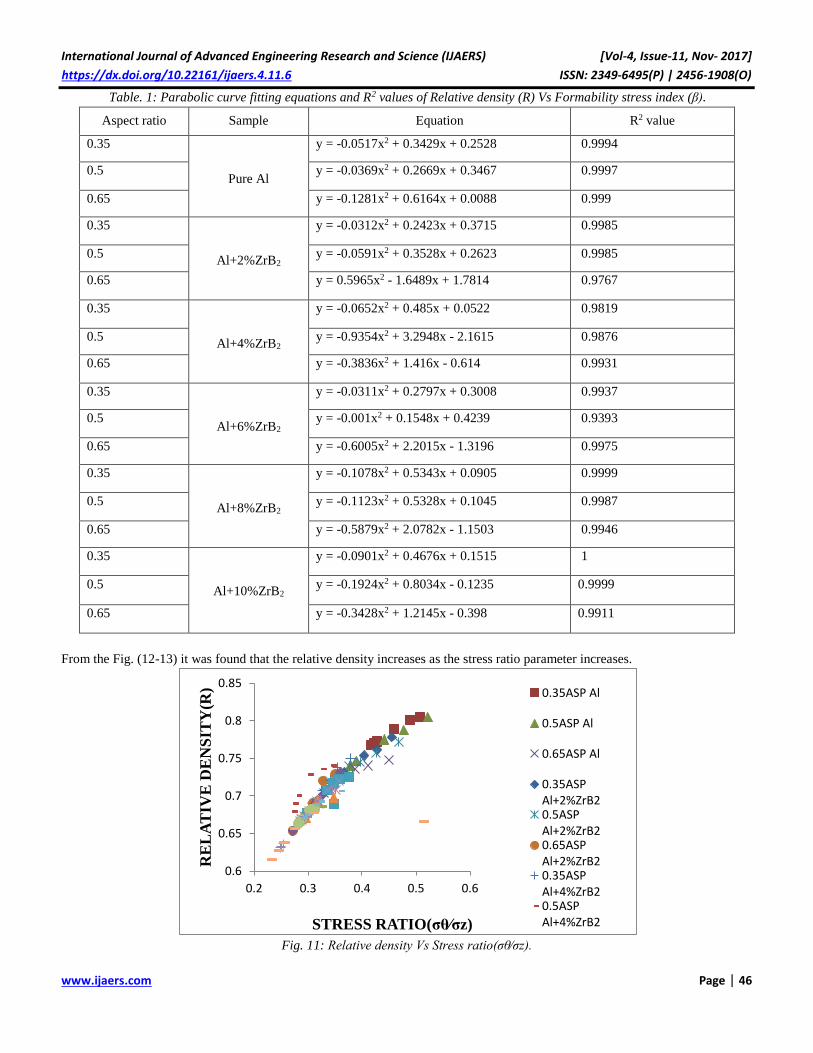
International Journal of Advanced Engineering Research and Science (IJAERS) [Vol-4, Issue-11, Nov- 2017]

https://dx.doi.org/10.22161/ijaers.4.11.6 ISSN: 2349-6495(P) | 2456-1908(O)

www.ijaers.com Page | 46

Table. 1: Parabolic curve fitting equations and R2 values of Relative density (R) Vs Formability stress index (β).

Aspect ratio Sample Equation R2 value

0.35

Pure Al

y = -0.0517x2 + 0.3429x + 0.2528 0.9994

0.5 y = -0.0369x2 + 0.2669x + 0.3467 0.9997

0.65 y = -0.1281x2 + 0.6164x + 0.0088 0.999

0.35

Al+2%ZrB2

y = -0.0312x2 + 0.2423x + 0.3715 0.9985

0.5 y = -0.0591x2 + 0.3528x + 0.2623 0.9985

0.65 y = 0.5965x2 - 1.6489x + 1.7814 0.9767

0.35

Al+4%ZrB2

y = -0.0652x2 + 0.485x + 0.0522 0.9819

0.5 y = -0.9354x2 + 3.2948x - 2.1615 0.9876

0.65 y = -0.3836x2 + 1.416x - 0.614 0.9931

0.35

Al+6%ZrB2

y = -0.0311x2 + 0.2797x + 0.3008 0.9937

0.5 y = -0.001x2 + 0.1548x + 0.4239 0.9393

0.65 y = -0.6005x2 + 2.2015x - 1.3196 0.9975

0.35

Al+8%ZrB2

y = -0.1078x2 + 0.5343x + 0.0905 0.9999

0.5 y = -0.1123x2 + 0.5328x + 0.1045 0.9987

0.65 y = -0.5879x2 + 2.0782x - 1.1503 0.9946

0.35

Al+10%ZrB2

y = -0.0901x2 + 0.4676x + 0.1515 1

0.5 y = -0.1924x2 + 0.8034x - 0.1235 0.9999

0.65 y = -0.3428x2 + 1.2145x - 0.398 0.9911

From the Fig. (12-13) it was found that the relative density increases as the stress ratio parameter increases.

Fig. 11: Relative density Vs Stress ratio(σθ⁄σz).

0.6

0.65

0.7

0.75

0.8

0.85

0.2 0.3 0.4 0.5 0.6

RE

LA

TIV

E D

EN

SIT

Y(R

)

STRESS RATIO(σθ⁄σz)

0.35ASP Al

0.5ASP Al

0.65ASP Al

0.35ASPAl+2%ZrB20.5ASPAl+2%ZrB20.65ASPAl+2%ZrB20.35ASPAl+4%ZrB20.5ASPAl+4%ZrB2

International Journal of Advanced Engineering Research and Science (IJAERS) [Vol-4, Issue-11, Nov- 2017]

https://dx.doi.org/10.22161/ijaers.4.11.6 ISSN: 2349-6495(P) | 2456-1908(O)

www.ijaers.com Page | 47

Fig. 12: Relative density Vs Stress ratio(σz/σm).

(a)

(b)

(c)

Fig. 15: Axial stress (σz) Vs Relative density (R) (a) 0.35

ASPR, (b) 0. 5 ASPR and (c) 0.65 ASPR

The Fig. 15(a-c) shows the plot of axial stress (σz) against

the relative density R. The experiment has been done with

preforms with initial densities ranging from 0.6 to 0.75 and

aspect ratios ranging from 0.35 to 0.65. Along with the

densification, the load bearing capability of the preforms

also increase, as is evident from the higher stress values in

the plot 15(a-c)

It was found that the preform with 10 % ZrB2 and 0.35

aspect ratio had densified more. Preforms with high initial

preform density had higher load bearing capacity and longer

0.6

0.65

0.7

0.75

0.8

0.85

1.3 1.5 1.7 1.9 2.1

RE

LA

TIV

E D

EN

SIT

Y(R

)

STRESS RATIO(σz/σm)

0.35ASP Al

0.5ASP Al

0.65ASP Al

0.35ASP Al+2%ZrB2

0.5ASP Al+2%ZrB2

0.65ASP Al+2%ZrB2

0.35ASP Al+4%ZrB2

0.5ASP Al+4%ZrB2

0.65ASP Al+4%ZrB2

0.35ASP Al+6%ZrB2

0

50

100

150

200

250

0.6 0.8 1

AX

IAL

STR

ESS(σ

z)

RELATIVE DENSITY

Pure Al

Al+2%ZrB2

Al+4%ZrB2

Al+6%ZrB2

Al+8%ZrB2

0

50

100

150

200

0.6 0.8 1

AX

IAL

STR

ESS(σ

z)

RELATIVE DENSITY

Pure Al

Al+2%ZrB2

Al+4%ZrB2

Al+6%ZrB2

Al+8%ZrB2

0

20

40

60

80

100

120

140

160

180

200

0.6 0.7 0.8

AX

IAL

STR

ESS(σ

z)

RELATIVE DENSITY

Pure Al

Al+2%ZrB2

Al+4%ZrB2

Al+6%ZrB2

Al+8%ZrB2

Al+10%ZrB2

International Journal of Advanced Engineering Research and Science (IJAERS) [Vol-4, Issue-11, Nov- 2017]

https://dx.doi.org/10.22161/ijaers.4.11.6 ISSN: 2349-6495(P) | 2456-1908(O)

www.ijaers.com Page | 48

strain to failure. This was due to the presence of lesser

number of pores.

IV. CONCLUSIONS

The porosity increased with increased quantity of ZrB2

reinforcement, as the ultra-hard ZrB2 particles in the

composite don’t allow the load applied while

compaction to close the pores.

The hardness of the composites increased with increased

amount of ZrB2 reinforcement in the composite.

The formability behaviors of sintered Al-ZrB2

composite preforms had been studied in this paper. The

formability stress index increased with increase in initial

preform fractional density and decreases with the aspect

ratios. A statistical fitting methods were to draw curves

between the relative density and axial strain, axial strain

and the formability stress index. The parabolic curve

fitting was found to give better prediction results. The

initiation of crack appeared at a very high fracture strain

for the compacts with higher value of the aspect ratio

and high initial preform density.

REFERENCES

[1] J. Mascarenhas, Powder metallurgy: a major

partner of the sustainable development, Materials

Science Forum, 455- 456 (2004), 857–860, doi:

10.4028/ www.scientific.net/ MSF.455-456.857.

[2] Dieter GE, Mechanical Metallurgy, New York:

McGraw-Hill 3rd ed., 1981.

[3] A. Riaz Ahamed , P. Asokan and S. Aravindan,

EDM of hybrid Al–SiCp–B4Cp and Al–SiCp–

Glassp MMCs, Journal Advance Manufacturing

Technol (2009) 44:520–528. DOI 10.1007/s00170-

008-1839-0.

[4] M. Ramulu, G. Paul and J. Patel, EDM surface

effects on the fatigue strength of a 15vol% SiCP/Al

metal matrix composite material, Composite

structures 54 (2001) 79-86.

[5] Sumathi, M., Selvakumar, N., & Narayanasamy,

R., Workability studies on sintered Cu-10SiC

preforms during cold axial upsetting, Materials and

Design, 39 (2012), 1–8, doi:

10.1016/j.matdes.2012.02.004

[6] Narayanasamy, R., Anandakrishnan, V., &

Pandey, K. S., Effect of carbon content on

workability of powder metallurgy steels, Materials

Science and Engineering A, 494 (2008), 337–342,

doi:10.1016/j.msea.2008.04.022

[7] Selvakumar N and Narayanasamy R., Phenomenon

of strain hardening behaviour of sintered

aluminium preforms during cold axial forming,

Journal of Materials Processing Technology, 142

(2003), 347-354, doi:10.1016/S0924-

0136(03)00605-8

[8] Harsh Saini, Irfan Khan, Sushil Kumar, Sahil

Kumar(2017).Optimization of Material Removal

Rate of WEDM Process on Mild Steel Using

Molybdenum Wire. International Journal of

Advanced Engineering, Management and Science

(ISSN: 2454-1311), 3(10), 1001-1005.

http://dx.doi.org/10.24001/ijaems.3.10.5

[9] Narayanasamy R, Ramesh T and Pandey KS.,

Some aspects on workability of aluminium–iron

powder metallurgy composite during cold

upsetting, Materials Science and Engineering,

A391 (2005), 418–426, doi:

10.1016/j.msea.2004.09.018

International Journal of Advanced Engineering Research and Science (IJAERS) [Vol-4, Issue-11, Nov- 2017]

https://dx.doi.org/10.22161/ijaers.4.11.7 ISSN: 2349-6495(P) | 2456-1908(O)

www.ijaers.com Page | 49

Study of Irrigation Water Supply Efficiency to

Support the Productivity of Farmers (Case Study

at Kobisonta North Seram Central Maluku

District) Hengky Jhony Soumokil, Obednego Dominggus Nara

Lecturer Polytechnic Ambon, Jl. Ir Putuhena Wailela – Ambon Indonesia

Abstract— The need of water is a major media of irrigation

in order to support the effectiveness of agricultural business

which is manifested as the supporting of food provision. The

purpose of this study is to analyze the amount of discharge

in each channel and the efficiency in Kobisonta irrigation

area, Seti North Seramsubdistrict, Central Maluku district

with area of 3,150 ha. The study was conducted on

secondary channels Kobisonta includes BKS7, BKS8,

BKS9, Kobisonta Secondary Channel includes BKS10,

BKS11, BKS12 and Seti Secondary Line includes BS1, BS2

and BS3

The water debit requirement in the rice field and the

efficiency in the irrigation area of Kobisonta was analyzed

by using the incoming debit - discharge method based on

flow velocity measurement. Providing irrigation water for

efficiently is not simple because many factors affect the way

and the process, besides that if the water supply and

irrigation on the channel is inefficient, then it can reduce or

decrease agricultural productivity.

From the result of actual debit analysis on channel BS3,

BKS9, BKS11, and BKS12, they are able to meet

therequirement of irrigation water thoroughly in irrigation

area. In BS1, BS2, BKS8 and BKS10 channels, actual

discharge has not been able to meet the irrigation water

needs in its irrigation area. The efficiency of irrigation

channels in Kobisonta Irrigation Area varies by channel.

According to the efficiency standard by the Directorate

General of Irrigation, the secondary Saluaran in Irrigation

Area is categorized as efficient where for BKS7 is 90%,

BKS8 is 97% and BS2 is 91%.

Keywords— discharge, efficiency, irrigation.

I. INTRODUCTION

Irrigation is an effort to supply and regulate water with the

purpose of agriculture supporting that can include surface

water irrigation, underground water irrigation, pump

irrigation and local irrigation. Kobisonta is located in East

Seram District Seti, Central Maluku district with a

population of 14,923. It is one of the rice production

centers.

The construction of Kobi weir which is located in the

village of Kobisonta, North Seram District Seti, Central

Maluku District which in this case, has a water catchment

area of 145.4 km2, is expected to meet the water needs for

irrigated rice fields of 3,150 ha. So here, researchers use the

object of research located in one of the villages located in

the Central Maluku District.

In supporting the water needs in the agricultural sector with

irrigation system, indeed there will be some problems that

arise. One of them is the loss of water that occurs in each

channel on the way to the rice field. This study is conducted

can give contribution in completing the existing irrigation

network study information, by focusing more on the

efficiency and effectiveness of irrigation network operating

system on the level of service of primary channel,

secondary and tertiary channels to water requirements in

rice crops.

II. LITERATURE REVIEW

The meaning of Irrigation

Irrigation is a watering activity on an agricultural land that

aims to create moist conditions in the root of the plant to

meet the water needs for plant growth. According to Basri,

1987 irrigation is the provision of water in plants to meet

the water needs for its growth. According to Karta Saputro,

1994 irrigation is an activity of supply and regulation of

water to meet the interests of Agriculture by utilizing water

from surface water and soil. According to Suharjono, 1994

irrigation is a number of water that is generally taken from

International Journal of Advanced Engineering Research and Science (IJAERS) [Vol-4, Issue-11, Nov- 2017]

https://dx.doi.org/10.22161/ijaers.4.11.7 ISSN: 2349-6495(P) | 2456-1908(O)

www.ijaers.com Page | 50

rivers or weirs that flowed through the irrigation system to

maintain balance the amount of water in the soil.

2.1 Irrigation Network

The irrigation network is the unity of the canals and

structures necessary for the regulation of irrigation water

from the provision, collection, distribution, delivery and

use. There are two kinds of irrigation networks:

1. The main irrigation network: irrigation network that is

located in an irrigation system, starting from main

building, main / mainline, secondary channel, and

tapping building and its complementary building.

a. Main / primary channel

b. Secondary irrigation channels

2. Tertiary Irrigation Network: a network that serves as a

water service infrastructure within a tertiary grid

consisting of a carrier channel called a tertiary channel,

a dividing channel called a Quaternary channel, and a

drainage channel and auxiliary channels.

2.2 Irrigation Efficiency

Irrigation efficiency shows the use of water that is the ratio

between the amount of water used and the amount of water

given expressed in percent (%).

𝐸𝑓𝑖𝑠𝑖𝑒𝑛𝑠𝑖𝐼𝑟𝑖𝑔𝑎𝑠𝑖 =𝑑𝑒𝑏𝑖𝑡𝑎𝑖𝑟𝑦𝑎𝑛𝑔𝑘𝑒𝑙𝑢𝑎𝑟 (𝑚3 /𝑑𝑒𝑡𝑖𝑘)

𝑑𝑒𝑏𝑖𝑡𝑎𝑖𝑟𝑦𝑎𝑛𝑔𝑚𝑎𝑠𝑢𝑘 (𝑚3/𝑑𝑒𝑡𝑖𝑘)×

100%(eq 1)

Estimated efficiency of irrigation is set as follows (KP-01,

1986: 10):

1. tertiary network = 80%

2. secondary network = 90%; and

3. primary network = 90%.

While the overall irrigation efficiency factor is 80% x 90%

x 90% = 65%.

2.3 Water Discharge

The amount of liquid that flowing through a cross-section of

flow per one unit of time is called flow discharge (Q).

Q = A ∙ V (eq.2)

2.4 Water Loss

Water loss is generally divided into 2 categories, among

others:

1. Loss of physical consequences where water loss occurs

due to water seepage in the channel and percolation at

farm level (paddy field); and

2. Operational loss occurs due to exhaust and excess water

discharges during channel operation and waste of water

used by farmers.

The loss of water on each inlet measurement (Inflow -

Outflow) is calculated as the difference between inlet and

outflow discharge. (IPB Water Management Research

Team, 1993: 1-05):

ℎ𝑛 = 𝐼𝑛−𝑂𝑛 (eq 3)

Table.1: Flow Velocity Measurement Method

2.5 Water Requirement

Parameters that is used in water demand analysis are:

1. Coefficient of plant (Kc)

The magnitude of Kc varies, in this study used the

numbers suggested by FAO (Irrigation Planning

Standards, KP-01 p. 164).

2. Irrigation efficiency (e)

The need for water in rice fields for rice crops can be

determined by the following factors (MawardiEman 2007:

103);

o How to prepare the land

o Water needs for plants / consumtive used

o Percolation and seepage

o Replacement of water layers

o Effective rainfall

2.6 How to prepare the land

Water requirements for land preparation were calculated

using the methods of Van de Goor and Zijlstra (1968) as

follows:

IR = M (e ^ k / (e ^ k-1) (eq 4)

2.7 Water requirements for plants / consumtive use

The water requirement for plants is water that is used up for

plant growth. This water requirement is calculated by

multiplying the crop coefficient with potential

evapotranspiration.

Etc= Kc x Etp (eq 5)

2.8 Effective rainfall

A. Water Requirement for Irrigation Irrigation water

demand in paddy field is calculated for rice-rice planting

pattern with the following conditions:

o Need for clean water in paddy fields (NFR):

NFR = ET c + P - Re + WLR (eq 6)

Depth (m) Velocity Observation Average Velocity

0.00 - 0.60 0.6d = V0.6d

0.2d

0.8d

0.2d

0.6d

0.8d

S

0.2d

0.6d

0.8d

0.60 - 3.00

3.00 - 6.00

> 6.00

= 0.5 (V0.2d + V0.8d)

= 0.25 (V0.2d + V0.6d + V0.8d)

= 1/10 (Vs + 3V0.2d + 2V0.6d + Vb)

International Journal of Advanced Engineering Research and Science (IJAERS) [Vol-4, Issue-11, Nov- 2017]

https://dx.doi.org/10.22161/ijaers.4.11.7 ISSN: 2349-6495(P) | 2456-1908(O)

www.ijaers.com Page | 51

o Irrigation water needs for rice (WRD):

IR = NFR / e (eq7)

o Irrigation water needs for crops (WRP):

IR = (ET c - Re) / e (eq 8)

The determination of effective rainfall is based on monthly

rainfall that is using R80, which means 20% probability is

unavailable. The amount of effective rainfall for rice plants

is 70% of the minimum monthly rainfall with a 5 year re-

period (Irrigation Network Planning, KP-01, 1986,165),

with the following equation:

Re = 0.7 × 1/15 × (R_80) (eq 9)

Effective rainfall is a plumper rainfall that falls in an area

and is used for growth crops.

III. METHOD

Star

Primary data

· flow velocity

measurement

· Geometric Channel

Measurements

Data collection

Secondary data

· Network Scheme

· Climatology Data

analysis

Finish

Fig.1: Flowchart Metodologi

3.1 Tools

The tools that are used in this study are: current meter,

meter roll, stopwatch, measuring ruler.

3.2 The Measurement Steps are:

Measurement Steps on the Ground:

1. Current Meter

Current velocity measurements are illustrated by the

following measurement procedures:

a) Measure the depth of the channel with the measuring

pole of the current meter device

b) Select the propeller corresponding to the channel depth,

so it can be used for some vertical dots ie (0.2h, 0.6h,

0.8h) where h is the channel depth.

c) The current meter is mounted on a static mast with a

depth of 0.2h, 0.6h, and 0.8h, then the measuring rod is

inputted into the water until the baseband is located at the

bottom of the duct with the propeller facing the flow

direction (water current).

d) The number of turns per unit of time, which occurs at

each water depth, is calculated.

3.3 Source of Data

Source of data used in this research are:

1. Primary Data

Primary Data is data obtained by measuring the

Geometric cross section of the velocity flow channel (V),

and the channel length (L).

2. Secondary Data

Secondary data obtained from other parties or from

existing reports and research, and which have relevance to

the issues discussed, including the number and types of

irrigation networks studied, the network scheme of the

P3A existing in the Kobisonta Irrigation Area, data on

water demand on irrigation area kobisonta, as well as data

from several government agencies related among others

Office of Public Works.

3.4 Data Analysis Technique

Data analysis techniques in this writing done through the

stages as follows:

1. Analyze flow velocity by measuring instruments Current

meters and or buoys.

2. Analysis of inlet and outflow discharge on secondary

channel kobisonta, channel kobisonta, and channel setunder

secondary, (equation 3).

3. Analysis of water loss in secondary channel kobisonta,

channel kobisonta, and secondary channel seti, by the

difference between inlet and outflow (equation 3)

4. Efficiency analysis on the secondary channel kobisonta,

channel kobisonta, and secondary channel seti (equation 1).

5. Analysis of water needs in rice plants in Kobisonta

Irrigation Area.

IV. RESULT

Description about the location

Administratively, Kobisonta Irrigation Area is located in

Kobisonta village, North Seramsubdistrict of Seti, Central

Maluku regency. This sub-district is an expansion of the

District of North Seram through the Regional Regulation

International Journal of Advanced Engineering Research and Science (IJAERS) [Vol-4, Issue-11, Nov- 2017]

https://dx.doi.org/10.22161/ijaers.4.11.7 ISSN: 2349-6495(P) | 2456-1908(O)

www.ijaers.com Page | 52

(Perda/region regulation) of Central Maluku Number 9 of

2010, with a population of 14,923 inhabitants. The village

of Kobisonta is one of the rice production area centers

where almost all the local people live as farmers. The

construction of Kobi Dam is located in Kobisonta Village,

North Seram District Seti, Central Maluku Regency. The

Kobi River has a water catchment area of 145.4 km2 on the

site dam position with a river length of 12.3 km.

Kobidam is expected to meet the water requirement for

irrigation 3.150 ha of rice fields equal to 31.5 km2.

Irrigation water management at farmer level in Kobiosonta

Irrigation Area conducted by Water User Farmers (P3A),

which is summarized into the Water User Farmers

'Margorejo'

The working area of this association is the Tertiary Plot

with a working area of 52 Ha. The source of water used

comes from WaiKobi's Bend water which is tapped through

the primary channel to the secondary door and then

distributed three secondary channels. The first secondary

channel is the Seti secondary channel that includes the areas

of BS.1, BS.2 and BS.3, the second secondary channel of

Kobisonta secondary channel covers the area BKS.7, BKS.8

and BKS.9 and for the secondary secondary channel

secondary channel Kobisonta's face covers the area of

BKS.10, BKS.11 and BKS.12.

4.1 Flow Rate Analysis In Irrigation Channels

Measurements of velocity on the irrigation can be done

directly by using a buoy or indirectly which usually uses a

current meter. Measurement of flow velocity in the

Kobisonta Irrigation area the researchers used the Current

Meter type C2 tool. Here the researcher uses propeller type

current meter, this type rotates to the horizontal axis.

The number of turns per unit time can be converted to

current velocity. To shorten the time and save costs,

measurements can be made only at some point on the

vertical, ie at 0.6 d; 0.2 d; and 0.8 d; with d is the flow

depth.

The average velocity performed on the intake door is done

by using two (2) points method because the depth of the

intake door ranges from 0.6 to 3 meters, where the average

velocity is the average of velocity at 0.2 and 0.8 depth.

Fig.2: Measurement method of flow velocity

The research that is conducted at the intake door by using

the Current Meter obtained the formula of the tool on the

propeller current meter type that is:

v = 0.2397.n + 0,018 ...... (n <1,01)

v = 0.2556 .n + 0.002 ...... (1.01≤n <8.06)

v = 0.2494 .n + 0,052 ...... (8.06≤n <9.82)

To prove the measurement data available with the formula

of the tool then the researchers will describe the example

calculation to get the value of speed on each segment:

Fig.3: Division of flow rate measurement segments in the

field

While the mean velocity on the secondary channel that the

researchers do only use the method one (1) point because

the depth is at 0.0 - 0.6 meters, which can only be used for

shallow water where the method of two or more points can

not be done. Speed is measured at 0.6 water depth.

Table.2: Data flow recapitulation dataon channel BS.2

Table.3: Average velocity on each channel

2 Sectional area of the flow For cross-sectional area of the

intake is obtained by multiplying the width of the intake

cross-sectional area by the depth of the intake channel.

Point Wide Depth Depth of mill number of Time

(m) (m) (m) (m) rounds (Sec) at Point Average

0 LW Left 0.30

0.28 0.28 0.30 0.60 96 40 0.615 0.615

0.56 0.28 0.30 0.60 84 40 0.539 0.577

0.84 0.28 0.30 0.60 93 40 0.596 0.568

1.12 LW Right 0.30

0.587Average

Velocity (m/sec)

Velocity

(m/sec)

Intake 0.203

BKS 7 1.0692

BKS 8 0.368

BKS 9 0.3077

BKS 10 0.5633

BKS 11 0.3517

BKS 12 0.3854

BS 1 0.4068

BS 2 0.5867

BS 3 0.5143

Channel code

International Journal of Advanced Engineering Research and Science (IJAERS) [Vol-4, Issue-11, Nov- 2017]

https://dx.doi.org/10.22161/ijaers.4.11.7 ISSN: 2349-6495(P) | 2456-1908(O)

www.ijaers.com Page | 53

Table.4: cross-sectional area of the intake door

4.3 Sectional area of the secondary channel

The recapitulation data of the cross-sectional area for the

entire channel in the Kobisonta Irrigation Area is included

in table 4

Table.5: Sectional area on the intake door

4.4 Flow Debit Analysis

Calculation of the discharge in the channel in Kobisonta

Irrigation area is intended to know how far the effectiveness

of these channels in fulfilling the water requirement for

paddy crop in paddy field. Based on the measurements with

current meter in the field obtained the flow of water of each

channel on the DI. Kobisonta as follows:

Table.6: Debit recapitulation data on each channel

4.5 Irrigation Efficiency

Table.7: Standard Efficiency Levels for Irrigation

Channels

From the results of research conducted then researchers get

the value of efficiency on each channel, which is

appropriate (equation 1):

Table.8: Percentage of Irrigation Efficiency

4.6 Water Loss

To calculate the amount of water loss that occurred in

secondary channel in Kobisonta Irrigation area, the

following equation is used :ℎ𝑛 = 𝐼𝑛−𝑂𝑛

Table.9: Percentage of Water Loss on DI Channels.

Kobisonta

Wide (w) Depth (d) Area (A)

(m) (m) (m2)

A1 1 0.95 0.95

A2 1 0.95 0.95

A3 1 0.95 0.95

A4 1 0.92 0.92

A5 1 0.89 0.89

A6 1 0.80 0.80

A7 1 0.83 0.83

A8 1 0.83 0.83

A9 1 0.72 0.72

A10 1 0.70 0.70

A11 1 0.58 0.58

A12 1 0.57 0.57

A13 1 0.57 0.57

Segmen

Area

(m2)

Intake 10.26

BKS 7 0.35

BKS 8 0.48

BKS 9 0.53

BKS 10 0.27

BKS 11 0.39

BKS 12 0.29

BS 1 0.40

BS 2 0.25

BS 3 0.24

Channel code

Area Velocity Discharge

(m2) (m/sec) (m3/sec)

Intake 10.26 0.203 2.083

BKS 7 0.35 1.0692 0.374

BKS 8 0.48 0.368 0.177

BKS 9 0.53 0.3077 0.163

BKS 10 0.27 0.5633 0.152

BKS 11 0.39 0.3517 0.137

BKS 12 0.29 0.3854 0.112

BS 1 0.40 0.4068 0.163

BS 2 0.25 0.5867 0.147

BS 3 0.24 0.5143 0.123

Channel code

Channel efficiency (%)

Primary 90

Secondary 90

Tertiary 80

Inflow Outflow efficiency

(m3/sec) (m3/sec) (%)

BS 2 0.126 0.148 85

BS 1 0.148 0.161 92

BKS 11 0.113 0.137 83

BKS 10 0.137 0.152 90

BKS 9 0.152 0.164 93

BKS 8 0.164 0.177 93

BKS 7 0.338 0.375 90

Channel code

Inflow Outflow Losses Percentage

(m3/sec) (m3/sec) (%) (%)

BS 2 0.126 0.148 0.022 15

BS 1 0.148 0.161 0.013 8

BKS 11 0.113 0.137 0.024 17

BKS 10 0.137 0.152 0.015 10

BKS 9 0.152 0.164 0.012 7

BKS 8 0.164 0.177 0.013 7

BKS 7 0.338 0.375 0.037 10

Channel code

International Journal of Advanced Engineering Research and Science (IJAERS) [Vol-4, Issue-11, Nov- 2017]

https://dx.doi.org/10.22161/ijaers.4.11.7 ISSN: 2349-6495(P) | 2456-1908(O)

www.ijaers.com Page | 54

4.8 Effective rainfall

Calculates effective rainfall for rice by 70% of R80 of time

in a period, with the following equation:𝑅𝑒 = 0,7 ×1

15×

(𝑅80)

4.9 Estimated evaporation

Evaporation is expressed as the evaporation rate given in

millimeters per day. Evaporative measurements of the water

surface can be done in several ways. The most used way to

know the evaporative volume of the free water surface is to

use an evaporating pan. The method used in kobisonta

irrigation area is using class evaporation pans tool. The

result of ET0 analysis using Software Cropwat 8.0

Table.10: Results of Effective Rainfall Recapitulation

Table.11: Calculation of ET0

4.10 Water requirements for land preparation

Calculation of water requirements during land preparation,

used methods developed by Van de Goor and Zijlstra

(irrigation planning standard KP-01, 1986) with the

formula:

IR = M (e ^ k / (e ^ k-1))

Table.12: Calculation of Water Requirement Processing

Period

4.11 Water requirements for each field

Water requirement for rice crops seen from the maximum

requirement that is at age of rice aged two months. The

results of field measurements obtained data on the water

requirement of each rice field plot in the age of paddy aged

0.5 months to 4 months as follows.

Table.13: Water Requirements for each Plot

4.12 Water Requirement (Q Actual) on Channels and

Rice Fields

R 80%

comparative 1/2 month

( mm ) number ( mm ) % (mm/15 day) ( mm/day )

Des 1 157.90

Jan 1 155.50 84.54 70.00 59.18 3.95

Jan 2 129.05 70.16 70.00 49.11 3.27

Peb 1 77.75 25.51 70.00 17.86 1.19

Peb 2 81.03 26.59 70.00 18.61 1.24

Mrt 1 125.85 76.76 70.00 53.73 3.58

Mrt 2 149.25 91.04 70.00 63.73 4.25

Apr 1 70.20 42.08 70.00 29.46 1.96

Apr 2 85.95 51.52 70.00 36.06 2.40

Mei 1 47.25 30.48 70.00 21.34 1.42

Mei 2 50.40 32.52 70.00 22.76 1.52

Jun 1 9.45 2.68 70.00 1.88 0.13

Jun 2 35.00 9.92 70.00 6.94 0.46

Jul 1 76.65 43.80 70.00 30.66 2.04

Jul 2 102.20 58.40 70.00 40.88 2.73

Ags 1 76.65 42.57 70.00 29.80 1.99

Ags 2 107.35 59.63 70.00 41.74 2.78

Sep 1 92.10 55.98 70.00 39.18 2.61

Sep 2 109.95 66.82 70.00 46.78 3.12

Oct 1 53.55 30.63 70.00 21.44 1.43

Oct 2 71.28 40.77 70.00 28.54 1.90

Nov 1 53.18 25.85 70.00 18.10 1.21

Nov 2 92.65 45.05 70.00 31.53 2.10

Dec 1 118.43 67.87 70.00 47.51 3.17

Dec 2 157.10 90.03 70.00 63.02 4.20

Re-RiceMonth

R 80%multiplier factor

ReRe-Rice

157.90

154.70

52.10

167.80

93.60

63.00

12.60

102.20

102.20

122.80

71.40

70.90

LP=(M*ek)/(e

k-1) mm/day

S=250 mm S=300 mm S=250 mm S=300 mm

Jan 3.88 4.27 2.00 6.27 1.13 0.94 9.27 10.28

Feb 4.55 5.01 2.00 7.01 1.26 1.05 9.78 10.77

Mar 5.39 5.93 2.00 7.93 1.43 1.19 10.43 11.40

Apr 4.86 5.35 2.00 7.35 1.32 1.10 10.02 11.00

May 4.68 5.15 2.00 7.15 1.29 1.07 9.88 10.87

Jun 3.96 4.36 2.00 6.36 1.14 0.95 9.33 10.34

Jul 4.15 4.57 2.00 6.57 1.18 0.98 9.47 10.48

Aug 4.63 5.09 2.00 7.09 1.28 1.06 9.84 10.83

Sep 4.56 5.02 2.00 7.02 1.26 1.05 9.78 10.78

Oct 5.20 5.72 2.00 7.72 1.39 1.16 10.28 11.26

Nov 4.30 4.73 2.00 6.73 1.21 1.01 9.58 10.59

Dec 4.21 4.63 2.00 6.63 1.19 0.99 9.52 10.52

T=45 day

mm/day

MonthEt0 E0=1.1*Et0 P M=E0+P

k=M*T/S

T=45 day

Plot extensive

Code 0.5 1 1.5 2 2.5 3 3.5 4 rice fields (Ha)

BS3 0.21 0.71 0.40 1.04 0.66 0.33 0.21 0 179.80

BS2 0.21 0.71 0.40 1.04 0.66 0.33 0.21 0 95.80

BS1 0.21 0.71 0.40 1.04 0.66 0.33 0.21 0 50.90

BKS12 0.21 0.71 0.40 1.04 0.66 0.33 0.21 0 72.00

BKS11 0.21 0.71 0.40 1.04 0.66 0.33 0.21 0 45.00

BKS10 0.21 0.71 0.40 1.04 0.66 0.33 0.21 0 84.70

BKS9 0.21 0.71 0.40 1.04 0.66 0.33 0.21 0 39.50

BKS8 0.21 0.71 0.40 1.04 0.66 0.33 0.21 0 26.30

Plot extensive

Code 0.5 1 1.5 2 2.5 3 3.5 4 rice fields (Ha)

BS3 0.04 0.13 0.07 0.19 0.12 0.06 0.04 0.00 179.80

BS2 0.02 0.07 0.04 0.10 0.06 0.03 0.02 0.00 95.80

BS1 0.01 0.04 0.02 0.05 0.03 0.02 0.01 0.00 50.90

BKS12 0.02 0.05 0.03 0.07 0.05 0.02 0.02 0.00 72.00

BKS11 0.01 0.03 0.02 0.05 0.03 0.01 0.01 0.00 45.00

BKS10 0.02 0.06 0.03 0.09 0.06 0.03 0.02 0.00 84.70

BKS9 0.01 0.03 0.02 0.04 0.03 0.01 0.01 0.00 39.50

BKS8 0.01 0.02 0.01 0.03 0.02 0.01 0.01 0.00 26.30

Water needd (Lt/s)

water needs of each field (m3/s)

International Journal of Advanced Engineering Research and Science (IJAERS) [Vol-4, Issue-11, Nov- 2017]

https://dx.doi.org/10.22161/ijaers.4.11.7 ISSN: 2349-6495(P) | 2456-1908(O)

www.ijaers.com Page | 55

The water requirements in the canals and areas in the study

were performed when the actual 2-month-old rice was

calculated by the following scheme:

Table.14: Comparison of water requirements in the plot

rice field with actual water discharge

Fig.4: Graph of Water Requirement comparisons

Based on the graph above, the actual debit on BS3, BKS9,

BKS11 and BKS12 channels can meet the overall

requirement of irrigation water in the irrigation area. In

BS1, BS2, BKS8 and BKS10 channels, actual discharge has

not been able to meet the irrigation water needs in its

irrigation area.

4.13 Discussion

The area of rice fields in Kobisonta irrigation area of 3,150

ha has three secondary channels namely kobisonta

secondary channel (BKS7, BKS8, and BKS9), secondary

channel faces kobsionta (BKS10, BKS11 and BKS12) and

secondary channel seti (BS1, BS2 and BS3) which take

water from Bend WaeKobi. Each of the secondary channels

studied has different irrigation areas, channel lengths, and

wet cross-sectional areas.

In the dry season the farmers in Kobisonta village still plant

rice, this is because the water supply in BendungWaeKobi

is considered still able to meet the needs of irrigation.

Management of irrigation water distribution that is less

good or optimal cause some of its debit channel is not

sufficient to meet the needs of irrigation of rice crops in the

village kobsionta.

Lacks of the farmer’s discipline in the distribution of water

were found in many fields. Distribution of irrigation water

in Kobisonta Village is done by opening the water gate as

high as possible without taking into account the water

requirement in every irrigation area.

At each of irrigation in secondary irrigation area kobisonta

has different efficiency value. According to Irrigation

Secondary Irrigation Planning Standart is said to be

efficient if the efficiency rate of irrigation above 90%.

Based on the results in Table 8 Channel BKS7 which has

irrigation area of 185.10 ha and channel length 697.55

meters with actual discharge 0.37528 m3 / s has a watering

efficiency of 90%. In BKS8 channel with 700 meters

channel length with actual discharge 0.17664 m3 / s has a

watering efficiency of 93%. In BKS10 channel which has

irrigation area of 39.5 ha with actual discharge 0.1639 m3 /

s has water efficiency of 93%. In BKS11 channel which has

an irrigation area of 84.7 ha with actual discharge of 0.1521

m3 / s has irrigation efficiency of 90% and In channel BS1

with irrigation area 50.9 ha and a length of 800 meter

channel with actual discharge 0.1611 m3 / watering by

92%. In BKS7, BKS8, BKS9, BKS10 and BS1 value

efficiency above 90% then the channel can be said to be

efficient.

In BS2 channel which has irrigation area 95,8 ha and

channel length 1000 meter with actual discharge 0,1478 m3

/ s has watering efficiency equal to 85%. And Channel

BKS11 with irrigation area 45 ha and channel length 700

meters with actual discharge 0.1372 m3 / s has 83%

efficiency value. Secondary channel BS1, and BKS11 value

of efficiency below 90%. Then the channels have an

efficiency value below the standard. This is due to the

amount of mud deposits along the channel and leaks along

the channel.

For the percentage of losses in each channel in the

Kobisonta Irrigation Area has a different percentage values

per channel. According to DPU Repulik Indonesia KP-03

(1986: 7), generally water loss in the irrigation network on

the secondary channel 5 - 10%.

Based on the results of the data in table 9 On the secondary

channel BKS7 the percentage value of water loss of 10%,

channel BKS8 percentage value of water loss of 7%,

channel BKS9 water loss percentage value of 7%, channel

BKS10 percentage value of water loss by 10% and

secondary channel BS1 percentage value of water loss of

Area Needs Water debit Actual debit

(Ha) (m3/sec/ha) (m3/sec)

BS 3 179.8 0.19 0.125

BS 2 95.8 0.1 0.148

BS 1 50.6 0.05 0.161

BKS 12 72 0.07 0.113

BKS 11 45 0.05 0.137

BKS 10 84.7 0.09 0.152

BKS 9 39.5 0.04 0.164

BKS 8 26.3 0.03 0.177

Channel code

International Journal of Advanced Engineering Research and Science (IJAERS) [Vol-4, Issue-11, Nov- 2017]

https://dx.doi.org/10.22161/ijaers.4.11.7 ISSN: 2349-6495(P) | 2456-1908(O)

www.ijaers.com Page | 56

8%. For BKS7, BKS8, BKS9, BKS10 and BS1 meet the

standard according to the Public Works Department.

In BKS11 channel the percentage value of water loss is

17% and BS2 channel value of water loss percentage is

15%, so for BKS11 and BS2 channels do not meet DPU

standard because water loss percentage value is below 5-

10%. This is due to the seepage on a part of the bottom of

the drained channel, the amount of soil deposits, sand, loads

of loads in the form of wood, foliage, the amount of garbage

and the theft of water made by farmers that slows the flow

of water in the secondary channel in the irrigation area

kobisonta.

Based on 15 comparisons of debit requirements with the

actual water debit, the actual debit on channel BS3, BKS9,

BKS11, and BKS12 able to meet the requirement of

irrigation water as a whole in irrigation area. In BS1, BS2,

BKS8 and BKS10 channels, actual discharge has not been

able to meet the irrigation water needs in its irrigation area

In water supply for irrigation, there needs to be efficiency

and effectiveness of water supply. Efforts that need to be

made to improve the efficiency and effectiveness of

irrigation are:

1. To reduce the impact of vegetation damage and channel

cracking in Kobisonta Irrigation Area it is necessary to

maintain by Margorejo P3A either regularly or

periodically on each channel.

2. Need to be socialized about the process of water

distribution by P3A to farmers so that farmers are

expected to be more disciplined in implementing

irrigation water taking schedule.

V. CONCLUSION AND SUGGESTIONS

5.1 Conclusions

Based on the results and discussion, then we obtained the

following conclusions:

1. The efficiency of discharge in every secondary channel in

Kobisonta Irrigation area has different value. On the

secondary channel BKS.7 efficiency value 90%, BKS.8

93% efficiency value, BKS.9 efficiency value 93%,

BKS.10 value of efficiency 90% and BS. 1 efficiency

value of 92% on average has met the efficiency standard

according to Planning Standards of Secondary Irrigation

Planning for the efficiency of irrigation above 90%.

While for secondary channel BKS.11 83% efficiency

value, and BS.2 85% efficiency value does not meet the

standard of efficiency because the average value of

efficiency on the channel is below 90%.

2. Total water loss in Kobisonta Irrigation area for

secondary channel BKS.7 10%, BKS.8 7%, BKS.9 7%,

BKS.10 10% and BS.1 8% have met the planning

criteria which is the standard of Public Works Service.

In general, water loss in irrigation networks in the 5-

10% secondary channel while in the 17% BKS.11

channel, and BS.2 15% has exceeded the water loss

planning criteria. This is due to the seepage of some of

the bottom of the eroded channel, the amount of soil

sediment (sedimentation), waste and also because of the

theft of water conducted by farmers resulted in the slow

speed of water flow in the secondary channel DI.

Kobisonta

5.2 Suggestions

1. The need for socialization to the water users farmers

(P3A) Margorejo to understand and adhere to the way of

distribution of irrigation water so as not to harm other

farmers.

2. To improve the efficiency and effectiveness of water

distribution there needs to be cooperation between the

Public Works Department and the P3A.

3. Margorejo P3A is expected to always review the

conditions of existing channels in the Kobisonta

Irrigation System and repair the damaged channels,

clean up the sludge, waste along the canal.

REFERENCES

[1] Anonymous, Irrigation Planning Standards (KP - 01).

Jakarta, 1986.

[2] Directorate General of Water Resources. 1986.

Irrigation Planning Standards. Jakarta.

[3] DPU Irrigation. 2004. Law No.7 on Water Resources.

Jakarta.

[4] DPU Indonesian Repulic KP-03 (1986: 7)

Kartasapoetra, A.G., 1994. Post-Harvest Handling

Technology. RinekaCipta, Jakarta.

[5] Saptana, Sumaryanto, Hendiarto, R.S. Rivai, Sunarsih,

A. Murtiningsih and V. Siagian. 2001. Engineering

Optimization of Irrigáis Water Allocation in Order to

Increase Food Products and Farmers Income.

AgroEconomy Bulletin, Vol 1 No. 3. Center for

Agricultural Socio Economic Research and

Development.

[6] Enock Dashu, P.(2017).Microbial Effect of Refuse

Dump on the Composition of Leafy Vegetables Grown

in the Vicinity of Dump Site Along River Benue,

Mubi Road, Yola. International Journal of

Environment Agriculture and Biotechnology(ISSN:

2456-1878).2(4), 1895-1899.10.22161/ijeab/2.4.54

International Journal of Advanced Engineering Research and Science (IJAERS) [Vol-4, Issue-11, Nov- 2017]

https://dx.doi.org/10.22161/ijaers.4.11.7 ISSN: 2349-6495(P) | 2456-1908(O)

www.ijaers.com Page | 57

[7] Sumaryanto and T. Sudaryanto, 2001. Paradigm

Change of Water Resources Utilization and Its

Implication on Food Production Development

Strategy. FAE. Volume 19, No. 2. Center for

Agricultural Socio Economic Research and

Development.

[8] Standart Irrigation planning, planning criteria of

irrigation network part KP-01 1998.

[9] Sudjarwadi, 1990. Theory and Practice of Irrigation.

Inter-University Center of ScienceTechnique, UGM,

Yogyakarta

[10] Triatmodjo, B. 2015. Applied Hydrology, Faculty of

Engineering, GadjahMada University, Yogyakarta

[11] Wusunahardja, P.J., Efficiency and Irrigation Water

Loss. Journal of Information Engineering, 1991.

International Journal of Advanced Engineering Research and Science (IJAERS) [Vol-4, Issue-11, Nov- 2017]

https://dx.doi.org/10.22161/ijaers.4.11.8 ISSN: 2349-6495(P) | 2456-1908(O)

www.ijaers.com Page | 58

The Air Flow Analysis of Coffee Plantation

Based on Crops Planting Pattern of the

Triangular Grid and Shackle of Wheel graphs

by using a Finite Volume Method Dafik, Muhammad Nurrohim, Arif Fatahillah, Moch. Avel Romanza P, Susanto

Mathematics Education Department, FKIP University of Jember, Jember, Indonesia

Abstract— Coffee bean is one of the Indonesia major

export commodity. Based on the data from the 2012,

Indonesia was ranked at third biggest coffee beans

exporter in the world, after Vietnam and Brazil. A coffee

land expansion have been done to increase the

productivity of coffee beans, however it is not so effective.

One of the factors that affect the productivity is a crops

planting pattern. A good crops planting pattern will make

a good air circulation and it will finally affect to the

productivity of coffee beans. We will use a finite volume

method to analyze the air flow of coffee plantation based

on the soil roughness level, crops planting pattern of the

triangular grid and shackle of wheel graphs. The

simulation process is carried out by using MATLAB and

FLUENT softwares. The result shows that the crops

planting pattern of triangular grid and shackle of wheel

graphs gives a better air circulation process in the coffee

bean plantation.

Keywords— Coffee Plants, Air Flow, Soil Roughness

Level, Triangular grid graph, Finite Volume Method.

I. INTRODUCTION

Coffee is one of the second largest export product of

Indonesia Country (Instituteof Education, Training and

Agricultural Extension; 1984).During 20 years the total

area and production of coffee plantations in Indonesia

have risen a significant improved. However, as an

exporter country, Indonesia is still left behind the other

countries such as Vietnam and Brazil(FAO, 2012),it is

due to the decrease of the coffee production. One of the

factors that affect the productivity is a crops planting

pattern. A good crops planting pattern will make a good

air circulation and it will finally affect to the productivity

of coffee beans.

In this research will be constructed a mathematical model

of differential equations of the air circulation on the

coffee plantation based on the soil of roughness level and

cropping pattern of the triangular grid and shackle of

wheel graphs of two dimensions shapes. The governing

equation for this model are the momentum equation and

the energy equation.

2

2

2

2

2

2

2

20 2

i

j

j

i

j

j

i

iji

x

v

x

v

x

v

x

vpguu

t

(1)

¶j0

¶t+Ñu

iuj=Ñ -pu

i'+2mu

i'-1

2ru

i'u

j'

æ

èçö

ø÷-

2m¶u

i'

¶xi

+1

2

¶ui'

¶xj

+¶u

j'

¶xi

æ

èç

ö

ø÷ +

¶uj'

¶xj

æ

èç

ö

ø÷ -

rui'u

j'¶u

i

¶xi

+1

2

¶ui

¶xj

+¶u

j

¶xi

æ

èç

ö

ø÷ +

¶uj

¶xj

æ

èç

ö

ø÷

(2)

where: is the density of air fluid, g is the acceleration

of gravity, p is the air pressure, is the viscosity of air

fluid, ij is displacement force, u and v are respectively the

average velocity direction of X axis and Y axis, 'u and

'v are respectively turbulent flow direction of X axis and

Y axis.

Mathematics model for air circulation of coffee

plantation is affected by profile of vertical’s air

velocity(Kindangen, 2005):

rr

y

x

x

v

v (3)

where:vy is the average air velocity at a height y,vris the

average air velocity at the height benchmark, x is the

distance between plants,xris the benchmark distance,

International Journal of Advanced Engineering Research and Science (IJAERS) [Vol-4, Issue-11, Nov- 2017]

https://dx.doi.org/10.22161/ijaers.4.11.8 ISSN: 2349-6495(P) | 2456-1908(O)

www.ijaers.com Page | 59

andαis the characteristic value of roughness. The model

formed will be simulated and analyzed by using

MATLAB and FLUENT software.

II. RESEARCH METHODS

The study is started by collecting some relevant

literatures and references to the coffee plant, fluid,

turbulent flow and finite volume method. It will be

designed a model of air circulation on the coffee

plantation based on the level of the soil of roughness and

cropping pattern of the triangular grid and shackle of

wheel graphs. Furthermore, the researcher will discretize

the model by using finite volume method of Quick

technique.

The simulation of air circulation will be carried out

by MATLAB and FLUENT softwares to analyze the

relation between the level of the soil of roughness and air

circulation on coffee plantation. Finally we test and

evaluate the programme simulation to know weather the

programming is doing well or not in obtaining the air

circulation of coffee plantation based on the level of the

soil roughness.

(a)

(b)

Fig.1: (a) Triangular Grid Graph Cropping Pattern,(b)

Shackle of Wheel Graph Cropping Pattern

III. RESULTSANDDISCUSSION

The simulation is done by comparing the soil

roughness level and the air circulation of the coffee

plantation. The soil of roughness level are 0,1; 0,5;

and0,9. The initial velocity ofaircirculationis1,2m/s. The

number of trees at cropping pattern of a triangular grid

and shackle of wheel graphs of the direction of X axis(px)

and the direction of Y axis (py) is10. By substituting the

level in the soil of roughness we get Figure2.

(a)

(b)

Fig.2: The air circulation on coffee plantation with

different level of soil roughness by MATLAB

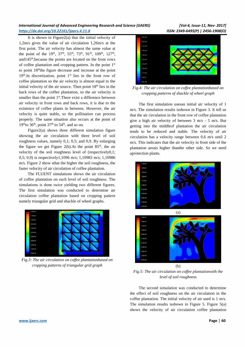
International Journal of Advanced Engineering Research and Science (IJAERS) [Vol-4, Issue-11, Nov- 2017]

https://dx.doi.org/10.22161/ijaers.4.11.8 ISSN: 2349-6495(P) | 2456-1908(O)

www.ijaers.com Page | 60

It is shown in Figure2(a) that the initial velocity of

1,2m/s gives the value of air circulation 1,26m/s at the

first point. The air velocity has almost the same value at

the point of the 19th, 37th, 55th, 73th, 91th, 109th, 127th,

and145th,because the points are located on the front rows

of coffee plantation and cropping pattern. In the point 1st

to point 18ththe figure decrease and increase at the point

19th.In discretization, point 1st lies in the front row of

coffee plantation so the air velocity is almost equal to the

initial velocity of the air source. Then point 18th lies in the

back rows of the coffee plantation, so the air velocity is

smaller than the point 1st.There exist a difference between

air velocity in front rows and back rows, it is due to the

existence of coffee plants in between. However, the air

velocity is quite stable, so the pollination can process

properly. The same situation also occurs at the point of

19thto 36th, point 37th to 54th, and so on.

Figure2(a) shows three different simulation figure

showing the air circulation with three level of soil

roughness values, namely 0,1; 0,5; and 0,9. By enlarging

the figure we get Figure 2(b).At the point 85th, the air

velocity of the soil roughness level of (respectively0,1;

0,5; 0,9) is respectively1,1096 m/s; 1,10983 m/s; 1,10986

m/s. Figure 2 show sthat the higher the soil roughness, the

faster velocity of air circulation of coffee plantation.

The FLUENT simulations shows the air circulation

of coffee plantation on each level of soil roughness. The

simulations is done twice yielding two different figures.

The first simulation was conducted to determine air

circulation coffee plantation based on cropping pattern

namely triangular grid and shackle of wheel graphs.

Fig.3: The air circulation on coffee plantationbased on

cropping patterns of triangular grid graph

Fig.4: The air circulation on coffee plantationbased on

cropping patterns of shackle of wheel graph

The first simulation usesan initial air velocity of 1

m/s. The simulation results isshown in Figure 3. It tell us

that the air circulation in the front row of coffee plantation

give a high air velocity of between 3 m/s - 5 m/s. But

getting into the middleof plantation the air circulation

tends to be reduced and stable. The velocity of air

circulation has a velocity range between 0,6 m/s until 2

m/s. This indicates that the air velocity in front side of the

plantation areais higher thanthe other side. So we need

aprotection plants.

(a)

(b)

Fig.5: The air circulation on coffee plantationwith the

level of soil roughness

The second simulation was conducted to determine

the effect of soil roughness on the air circulation in the

coffee plantation. The initial velocity of air used is 1 m/s.

The simulation results isshown in Figure 5. Figure 5(a)

shows the velocity of air circulation coffee plantation

International Journal of Advanced Engineering Research and Science (IJAERS) [Vol-4, Issue-11, Nov- 2017]

https://dx.doi.org/10.22161/ijaers.4.11.8 ISSN: 2349-6495(P) | 2456-1908(O)

www.ijaers.com Page | 61

with a large level ofsoil roughness of 0,9 is 2 m/s to 10

m/s, even reaches20 m/s. It endangerous the coffee

plantation as the higher the air circulation cause a bad

pollination of coffee plantation. It also cause many coffee

plantsflowers are falling down. So the productivity of

coffee bean will be low. Figure 5(b) shows the velocity of

air circulation coffee plantation with a lowlevel of soil

roughness of 0,1 is 0,5 m/s to 10 m/s. The lower the air

circulation give a good pollination of coffee plantation,

then it will gain a good productivity of coffee beans.

The velocity a average of air circulationof coffee

plantationtaken from coffee field is1,27m/s. while the a

average of air velocityof simulation results on the first

rows is1,25927m/s. It shown that the simulation is

relatively accurate. The errorand relative error values is

respectively0,01073and0,85%.

IV. CONCLUSIONS

It can be concluded that the level of soil roughness

affect to the air circulationof coffee plantation. The higher

the level of soil roughness the higher air circulation of

coffee plantation. The crops planting pattern of triangular

grid and shackle of wheel graphs give a better air

circulation process in the coffee bean plantation. A

cropping pattern in a plantation area of low air circulation

velocity, thesoil roughness level should be highto have

good air circulation. In this research we do not involve a

protection tree. It will be more challenging if it is also

considered a protection tree with a different cropping

patterns for further research. Apart from this, the other

researcher can study the effect ofthe humidity and soil of

slopeto the air circulation of coffee plantation.

REFERENCES

[1] Anonimous. 1984. Coffee. A center of Education,

Training, Counseling, Jakarta, Indonesia.

[2] Kindangen. 2005. The Investigation of Air Flow

Pattern of skyscraper Building of the constrain of

Front and Back Burrier of the building. Science

Journal, Vol. 11 Issue 4, p20-31.

[3] Muhidong, J., Mursalim, & Rahman, A. 2013. The

effect of air flow rate on single-layer drying

characteristics of Arabica coffee, International Food

Research Journal, October 2013, Vol. 20 Issue 4,

p1633.

[4] Najiyati, S. dan Danarti. 2001. Coffee, Plant

Copping, Post Harvest Management. XI Edition.

PenebarSwadaya, Jakarta, Indonesia

[5] Nilnont, W. dkk. 2012. Finite element simulation for

coffee (Coffea arabica) drying 269,, Food &

Bioproducts Processing: Transactions of the

Institution o, April 2012, Vol. 90 Issue 2, p341.

[6] Streeter, V. L. & Wylic, E. B. 1986.Fluid Mechanic.

(Eight Edition). Jakarta: Erlangga, Indonesia.

[7] Versteg, H. K. & Malalasekera, W. 1995.An

Introduction to Computational Fluid Dynamics :

The Finite Volume Method. Loughborough:

Longman Scientific & Technical.

[8] White, F. M. 1994, Fluid Mechanic. (Eight Edition).

Jakarta: Erlangga, Indonesia.

International Journal of Advanced Engineering Research and Science (IJAERS) [Vol-4, Issue-11, Nov- 2017]

https://dx.doi.org/10.22161/ijaers.4.11.9 ISSN: 2349-6495(P) | 2456-1908(O)

www.ijaers.com Page | 62

Seismic Study at Subba Oil Field Applying

Seismic Velocity Analysis Nawal Abed Al-Ridha1, Zahraa Shakir Jassim2

Department of Geology, College of Science, University of Baghdad, Baghdad. Iraq

Abstract— This research is seismic interpretation of two-

dimensional seismic data from oil exploration company in

Subba oil field. The field data process for the purpose of

interpretation, synthetic seismogram was done for the

well (Su-7) by using the sonic log and seismic velocity,

where the seismic reflectors were picked up (Nhr Umr,

Shuaiba, Zubair and Ratawi). Time and depth maps were

prepared, showing convex structure with a north-south

axis in the center of the study area, with two main dome

at northern and southern of the study area. Velocity

model from which velocity maps (Average velocity, and

interval velocity) were drawn. Seismic inversion

technique is used to shows the units within Formations

and delineate the increase or decrease of porosity in the

Nhr Umr and Zubair Formations.

Keywords— Velocity analysis, Seismic attribute, Subba

oil field.

I. INTRODUCTION

The geophysical techniques that most widely employed

for exploration are the seismic, gravity, magnetic, electric,

and electromagnetic methods. Less common method

involves the measurement of radioactivity and

temperature at or near the Earth's surface and in the air

[1]. The reflection method is depending on the study of

the elastic waves reflected from the interface between two

geological layers. The reflection method is used

exclusively for petroleum prospecting; it is more suitable

in areas where the oil is in structural traps, but also it is

useful for locating and detailing certain types of

stratigraphic features [2], reflection technique measures

the arrival time of seismic wave to travel from a source at

the Earth's surface down into the ground where it's

reflected back to a receiver which is located near the

surface. The seismic wave can be generated on the ground

by a near-surface explosion of dynamite, weight dropping

and vibrate [3]. The studied area is located south Iraq

between provinces of Basra, Dhi Qar and Almuthanna, as

shown in Figure (1). The aim of this research is using

velocity model and maps (vertical and horizontal average

velocity slices) to show variation of seismic velocities,

acoustic impedance and total porosity for Nahr Umr and

Zubair Formations.

Fig.1: Location map of study Area (Subba field )

II. DATA PROCESSING

Geophysical data processing is the use of computers for

the analysis of geophysical data. a major task in

geophysics is to determine as much as possible about the

constitution of the interior of the earth, [4]. we will

explain how to obtain the field data used and how to

process this data.

Processing steps:

1. Reformat applications: Field data are recorded in a

multiplexed mode using a certain type of format [5].

2. Geometry update: is an update of the field records

received from seismic teams in the field by sps file

containing the information recorded in the field such

as the values of (x , y , elevation and location …).

3. Static up date: is a correction of the delayed waves.

and eliminates the effect of differences in earth's

surface- level elevations.

4. Gain applications: is a time-variant scaling in which

the scaling function is based on a desired criterion

5. Noise attenuation: is classified into two categories,

random noise and coherent noise [6], as shown in

Figure (2).

International Journal of Advanced Engineering Research and Science (IJAERS) [Vol-4, Issue-11, Nov- 2017]

https://dx.doi.org/10.22161/ijaers.4.11.9 ISSN: 2349-6495(P) | 2456-1908(O)

www.ijaers.com Page | 63

Fig.2: types of noise

6. Deconvolution: is aimed at improving temporal

resolution by compressing the effective source

wavelet contained in the seismic trace to a spike

(spiking deconvolution).

7. Common - midpoint (CMP) Sorting: is the most

important data-processing application in improving

data quality. The principles involved have already

been discussed along with the field procedures used

to acquire the data, [7].

8. Normal-moveout correction: the velocity field is

used in normal moveout (NMO) correction of CMP

gathers, based on the assumption that, in a CMP

gather reflection travel times as a function of offset

follow hyperbolic trajectories, the process of NMO

correction removes the moveout effect on travel

times, [8].

9. Residual statics corrections: is one additional step in

conventional processing of land and shallow-water

seismic data before stacking [9].

10. Stacking: is one of the most advanced stages in the

treatment of seismic data, It aims primarily at

improving the quality of these data, Stacking

depends heavily on velocity derived from velocity

analyzes, It is applied after the procedures of the

NMO corrections, for best seismic sections, as

shown in Figures (3)

11. Velocity analysis: normal moveout is the basis for

determining velocities from seismic data. Computed

velocities can in turn be used to correct for NMO so

that reflections are aligned in the traces of a CMP

gather before stacking, as shown in Figure (5)

Fig.3: seismic section stack, A) old pick, B) new pick,

showing the changes in many places

Fig.4: A) Semblance panel, B) NMO-Corrected gather,

the wave field is flat, C) Un-corrected gather, D) The

area of stack to define the velocity.

III. SYNTHETIC SEISMOGRAM

The subsurface mapping and enhanced by the correlation

of seismic data with borehole data using the synthetic

seismogram, explain synthetic seismogram for well Su-7

where the density log, sonic log and check shot, as shown

in Figure (5)

International Journal of Advanced Engineering Research and Science (IJAERS) [Vol-4, Issue-11, Nov- 2017]

https://dx.doi.org/10.22161/ijaers.4.11.9 ISSN: 2349-6495(P) | 2456-1908(O)

www.ijaers.com Page | 64

Fig.5: Synthetic seismogram

IV. TWO WAY TIME (TWT) MAP

(TWT) map have been constructed from the picked

horizons Nahr Umr and Zubair Formations with contour

interval (20 msec).

The TWT values of Nahr Umr Formation are increasing

in the direction of the north-east and decreasing in the

south-west. at the south of subba field have small

structure at Su-8 well, and Zubair Formation shown

structure in the north part of study area, as shown in

Figures (6),(7)

Fig.6: Two way time maps of Nahr Umr formation

Fig.7: Two way time maps of Zubair Formation

V. VELOCITY MODEL

Velocity models are key components of seismic imaging,

and consequently, to reservoir description and geo

mechanical analysis.

Velocity model has been created by inserting surfaces

which were picked in time domain and well tops of Nahr

Umr, and Zubair horizons, the average velocity model

explain the change toward the basin, the velocity decrease

to north-east and increase to the south-west of the field, as

shown in Figure (8).

Fig.8: Velocity model of NahrUmr and Zubair

Formation

International Journal of Advanced Engineering Research and Science (IJAERS) [Vol-4, Issue-11, Nov- 2017]

https://dx.doi.org/10.22161/ijaers.4.11.9 ISSN: 2349-6495(P) | 2456-1908(O)

www.ijaers.com Page | 65

VI. VERTICAL AVERAGE VELOCITY SLICES

-In line slice:

The average velocity values decrease at the top of the

Nahr Umr Formation to the east at well Su-8, and low of

the average velocity values in Zubair Formation to the

same direction, the increase of values at the bottom of the

Ratawi Formation, as shown in Figure (9).

Fig.9: Vertical average velocity slices (In line slice)

-Cross line slice:

The cross line slice explain the lateral changes along of

the field shown the average velocity values decrease at

the top of the Nahr Umr to the north-east part especially

at wells Su-5 and Su-10 and continue low velocity zone in

Top Zubair and Ratawi Formation in same direction, as

shown in Figure (10).

Fig.10: Vertical average velocity slices (Cross line slice)

VII. Horizontal average velocity slice

Horizontal average velocity slice decrease toward the

north-east part of the field, and low average velocity

appears at boreholes area, and the velocity values increase

toward south-west, as shown in Figure (11) .

Fig.11: Horizontal average velocity slice

VIII. VELOCITY MAPS

Fig. 12: Average velocity map of Nahr Umr Formation

1. Average velocity map:

It's obtained from dividing the total distance travelled by

the wave by the time spent in [10]. The average velocity

maps of Nahr Umr and Zubair Formations explain the

increase and decrease in velocity, of Nahr Umr Formation

map the values are ranged from 3420 to 3870 m/s, having

closure average velocity in contour value 3550 m/s to the

north of field, where most of the oil wells were drilled.

Nahr Umr

Zubair Ratawi

Nahr Umr

Zubair Ratawi

International Journal of Advanced Engineering Research and Science (IJAERS) [Vol-4, Issue-11, Nov- 2017]

https://dx.doi.org/10.22161/ijaers.4.11.9 ISSN: 2349-6495(P) | 2456-1908(O)

www.ijaers.com Page | 66

The average velocity increase in velocity values in the

southern part and a decrease in the northern part, and

Zubair Formation the average velocity values are ranged

from 3500 to 3950 m/s, having closure average velocity

in contour value 3580 m/s to the north of field, as shown

in Figures (12),(13)

Fig. 13: Average velocity map of Zubair Formation

2. RMS velocity map:

Is defined as the square root of the average, can be

calculated from the interval velocity data [10].

The RMS velocity maps extracted from processing data,

Nahr Umr Formation map, the values are ranged from

3450 to 4350 m/s, having many closures to the north of

the field, between contour values (3400-4000 m/s), when

the oil wells were drilled, the velocity values decrease to

the north-east part and increase to the south-west part, and

Zubair Formation map explain the values range from

3550 to 4350 m/s, shown many closure of cantor interval

in center field, between contour values (3500-4100 m/s),

and having many smaller closure distributed to the south

of field, as shown in Figures (14),(15).

Fig. 14: RMS velocity map of Nahr Umr Formation

Fig. 15: RMS velocity map of Zubair Formation

IX. DEPTH MAPS

Depth estimation can be done via a wide range of existing

methods, but which can be separated into two broad

categories (direct time-depth conversion and velocity

modeling for time-depth conversion), [11].

International Journal of Advanced Engineering Research and Science (IJAERS) [Vol-4, Issue-11, Nov- 2017]

https://dx.doi.org/10.22161/ijaers.4.11.9 ISSN: 2349-6495(P) | 2456-1908(O)

www.ijaers.com Page | 67

Fig. 16: Depth map of Nahr Umr Formation

Nahr Umr Formation map explain the depth increasing to

the north-east part a depth of 2850 m, and the depth is

reduced toward the crest of the structure reaching a value

of 2450m near wells drilling, and depth map of Zubair

Formation is Match description to Nahr Umr depth map,

where the depth increasing to the north-east part a depth

of 3300 m, and the depth decrease toward the south-west

reaching to 2500 m, as shown in Figures (16),(17)

Fig. 17: Depth map of Zubair Formation

X. ISPACH MAP

Isopach maps constructed by subtracting the depth value

of two different horizons at each shot point, [12].

Thickness map of Nahr Umr Formation represent the

interval limited between top of Nahr Umr and the top of

Zubair using a contour interval of 5m. This map shows

the increasing in thickness to the south-west, and south

part of the area where a maximum thickness of 263m, and

the thickness decreases towards the north-east of the area

reaching a value of 203m, Thickness map of Zubair

Formation is the interval limited between top of Zubair

and the top of Ratawi using a contour interval of 10 m.

and the thickness decreases to the south of the area

reaching a value of 438 m, and the increasing in thickness

to the north, where a maximum thickness of 478m to the

north, as shown in Figures (18),(19).

International Journal of Advanced Engineering Research and Science (IJAERS) [Vol-4, Issue-11, Nov- 2017]

https://dx.doi.org/10.22161/ijaers.4.11.9 ISSN: 2349-6495(P) | 2456-1908(O)

www.ijaers.com Page | 68

Fig. 18: Thickness map of Nahr Umr Formation

Fig. 19: Thickness map of Zubair Formation

XI. SEISMIC INVERSION

The seismic inversion is applied on the line Sl-21 and

well Su-7, the result shows the low acoustic impedance in

green color show high porosity, and the violet color is

high acoustic impedance show low porosity. The

inversion section show the Nahr Umr reservoir divided

into three units and separate by one cap rock, and Zubair

reservoir divided into nine units and separate by four cap

rocks, as shown in Figure (20).

Fig.20: Seismic inversion section

The relationship between acoustic impedance and

porosity, as shown in Figure (21), where the increased

porosity to the Nahr Umr and Zubair Formations with

decreased in acoustic impedance, and the porosity

decreased when there is cap rock .

Fig.21: Cross plot show the relationship between acoustic

impedance and total porosity

XII. CONCLUSIONS

1. Seismic information indicates of that the area is not

affected by the fault system.

2. Time and depth maps explain the dipping of the

horizons to the south of field, and have high

structure to the north of field in drilling wells .

3. The average velocity maps of the Nahr Umr and

Zubair Formations are provided by using velocity

International Journal of Advanced Engineering Research and Science (IJAERS) [Vol-4, Issue-11, Nov- 2017]

https://dx.doi.org/10.22161/ijaers.4.11.9 ISSN: 2349-6495(P) | 2456-1908(O)

www.ijaers.com Page | 69

models. These maps show a decrease of average

velocity in the north part which due to the high

porosity and increases in the south part direction for

Nahr Umr and Formations, The average velocity

values affected by thickness and porosity .

4. RMS velocity of Nahr Umr and Zubair Formations

contain many closures in the central field.

5. Isopach maps explain Nahr Umr reflector was

increase in thickness in the south and decrease in the

north, Zubair reflector: Increase in thickness in the

north and decrease in the south.

6. Seismic inversion process was used to deduce the

reservoir units and total porosity, Nahr Umr

reservoir as shown divided to three units, and Zubair

reservoir divided into nine units and increasing of

the total porosity when the acoustic impedance

decreasing.

ACKNOWLEDGEMENTS

Praise is to Allah who guided us and prayer and peace be

upon the messenger of Allah Muhammad bin Abdu

Aullah.

I would like to express my appreciation and deep

gratitude to my supervisor, Prof. Dr. Nawal Abed Al-

Ridha , for her unwavering support ,collegiality and

encouragement at all stages of this work.

The researcher is grateful to the Department of Geology

at the University of Baghdad for providing opportunities

and facilities for the completion of this research.

I am so grateful to the Oil Exploration Company and its

managers for providing me all the facilities and

information that helped me in performing this research.,

especially to Mr. Jameel R. Kamoona , Mr. Muthana

Dawood, Miss. Ryhab Fadl Mahde, Mr. Suhail Ubaid

Muhsin, Mr. Salar Hasan, Mr. Amar Ahmed Jabir, Mr.

Mohammed Hashim Jiter, and Mr. Muhnd Ahsan .

Also, I present my greatest thanks and gratitude to

everyone in my family for their encouragement and

support .

REFERENCES

[1] Dobrin, M. B. and Savit, C. H., 1988: Introduction

to geophysical prospecting, 4th ed, McGraw-Hill

public., New York ,730 p.

[2] Al-Sinawi, 1981: Introduction to Applied

Geophysics, first ed., 142p.

[3] Dobrin, M. B., 1960: Introduction to geophysical

prospecting, 2nd ed McGraw– Hill. Int. co.,

International Student Edition, 446p.

[4] Claerbout, J. F., 1985: Fundamentals of Geophysical

Data Processing with applications to petroleum

prospecting, Department of Geophysics, Stanford

University, 266 p.

[5] Yilmaz, O., 1987: Seismic data processing, SEG

series: Investigation Geophysics, V.2, 526 p.

[6] Sengbush, R.L., 1983: Seismic exploration methods:

Internat. Human Res. Dev. Corp., Boston.

[7] Sheriff, R.E. and Geldart, L.P. 1995: Exploration

Seismology, 2nd edition. New York: Cambridge

University Press. 592 P .

[8] Mayne, W. H., 1962: Common-reflection-point

horizontal data stacking techniques: Geophysics, 27,

927-938.

[9] Taner, M. T., Koehler, F., and Alhilali, K. A., 1974:

Estimation and correction of near- surfaceTime

anomalies: Geophysics, 41, 441-463.

[10] Alsadi H. N., 2017: Seismic Hydrocarbon

Exploration 2D and 3D Techniques, Advances in

Oil and Gas Exploration & Production. Baghdad:

Data Processing Section Ministry of Oil. 331 P.

[11] Etris, E. L., Crabtree, N. J., and Dewar, J., 2001:

True Depth Conversion, Canada Society of

Exploration Geophysicists, pp. 11-22.

[12] McQuillin, R., Bacon, M, and Barclay, W.,

1984:An Introduction to Seismic Interpretation,

Graham and Trotman, 287p.

International Journal of Advanced Engineering Research and Science (IJAERS) [Vol-4, Issue-11, Nov- 2017]

https://dx.doi.org/10.22161/ijaers.4.11.10 ISSN: 2349-6495(P) | 2456-1908(O)

www.ijaers.com Page | 70

Peculiarities of a Colloidal Polysaccharide of

Newly Isolated Iron Oxidizing Bacteria in

Armenia Levon Markosyan1,*, Hamlet Badalyan2, Arevik Vardanyan1, Narine Vardanyan1

1Institute of Microbiology of SPC “Armbiotechnology” of the NAS of Armenia, Yerevan, 0056, Armenia 2Physical Ecology Laboratory of the Yerevan State University, Yerevan, 0025, Armenia

Abstract—Microorganisms belonging to different

systematic and physiological groups produce various

intra- and extracellular polysaccharides, which both play

an important role in the life of microorganisms and have

great practical application. Iron and sulfur oxidizing

bacteria produce capsular (EPS) and colloidal

polysaccharides. At present the properties and functional

role of EPS are well studied. However, the properties of

the colloidal polysaccharides produced by iron oxidizing

bacteria have not been sufficiently explored. A new iron

oxidizing bacteria Leptospirillum ferriphilium CC was

isolated from sulfide ores of Armenia. Its morphological

and physiological features have been studied. A colloidal

polysaccharide has been isolated with the use of an

original method developed by the authors, and its physical

and chemical properties have been studied. It has been

shown that the colloidal polysaccharide consists of three

different monomers- glucose, fructose, mannose..

Investigations with a complex method of optical

polarization microscopy and analytical programs allowed

determining the size, shape change, perimeter, degree of

hydratation and crystallization at 0.07% and 0.04% of

polysaccharide concentration. It was shown that the size of

a polysaccharide colloidal particle does not much depend

on polysaccharide concentration, however, the number of

identical colloidal formations is dependent on the

concentration of polysaccharide.

Keywords— cell morphology: colloidal polysaccharide:

iron oxidizing bacteria.

I. INTRODUCTION

Microorganisms, like eukaryotes and prokaryotes produce

polysaccharides, with different biological, chemical,

physical properties and functional activity. Iron and sulfur

oxidizing chemolithotrophic bacteria produce itra- and

exopolysaccharides. The properties of the intracellular

polysaccharides - lipopolysacchardes (LPS) of iron and

sulfur oxidizing bacteria have been studied. It was revealed

that the inter-specific diversity as well as the conditions of

cultivation and sources of energy define various properties

of LPS [1-7]. Generally the exopolysaccharides produced

by the above-mentioned bacteria are subdivided into

capsular and soluble/colloidal forms. Extensive research

undertaken in the past decades has been focused on

understanding the properties of the exopolysaccharides

contained in the extracellular substances (EPS) including

Acidihiobacillus ferrooxidans, Leptospirillum ferriphilum,

Leptospirillum ferrooxidans and formig a capsule around

the bacterial cell. EPS play an essential role for the

formation of a biofilm, which mediates adhesion of cells to

the minerals surface and form a cohesive three-dimensional

polymer interconnecting and immobilizing cells in the

process of bioleaching by iron and sulfur-oxidizing

bacteria. An important role of capsular polysaccharides as

a fundamental structural element of the EPS, determining

the mechanical stability of biofilm was disclosed [8-12].

However, the properties of colloidal

polysaccharides produced by iron and sulfur oxidizing

chemolithotrophic bacteria remains understudied. The

objective of the present study is to investigate the

properties of a colloidal polysaccharide of the iron

oxidizing chemolithotrophic bacteria Leptospirillum

ferriphilum CC newly isolated in Armenia.

II. MATERIALS AND METHODS

Bacterial culture and media. The Leptospirillum

ferriphilum CC was isolated from natural biotopes of

sulfide ores in Armenia.Cultivation was carried out in 9K

liquid medium with ferrous iron as a sources of energy at

37°C for 5-7 days.

Identification of strain. The isolated strain was identified

both by morphological, physiological properties [14] and

by the sequencing of 16S rRNA The primary analysis of

the data was carried out using the BLAST program. The

phylogenetic tree was constructed with the help of MEGA

6.06 and nighbor-joinig, and boot star programs.

Izolation of colloidal polysaccharide. The colloidal

polysaccharide produced by L. ferriphilum has been

International Journal of Advanced Engineering Research and Science (IJAERS) [Vol-4, Issue-11, Nov- 2017]

https://dx.doi.org/10.22161/ijaers.4.11.10 ISSN: 2349-6495(P) | 2456-1908(O)

www.ijaers.com Page | 71

isolated according to the method developed by the authors.

The isolation protocol is summarized in Fig 3.

Determination of the chemical composition of the

colloidal polysaccharide. Chemical composition of the

colloidal polysaccharide was analyzed after hydrolysis by 2

N HCl at 100°C for 2 hours by high performance liquid

chromatography (HPLC) on the Shimidzu 2010 C

analyzer, column ULTKON , P5-80-H 2 x 250 mm, the

mobile phase – 0.1 mM аcetat buffer/acetonitril-1:5, pH

5.8, flow rate 1ml/min. Measurements were made by RI.

Properties of colloidal formation. Properties of colloidal

formation of polysaccharide were studied by a complex

method combining optical polarization microscopy and

analytical programs LobViEW15 and WOVA [15, 16].

III. RESULTS AND DISCUSSION

Investigations of morphological properties of the isolated

iron oxidizing bacteria by light and optical polarization

microscopy and analytical programs disclosed that the cells

of the their area is 7033 μm, the length is 125μm, perimeter

is 462 μm and the shape of the cells is 0.0392.The

observed scatter of the morphological parameters of L.

ferriphilum is due to the non-synchronous growth of

culture in the population (Fig.1,Tabl. 2).

Fig.1: Microphotography of L. ferriphilum the

investigated bacteria have a curve rod- shape,

Based on the morphological and physiological

characteristics, as well as on the sequence of nucleotides in

16SrRNA, the isolated strain was identified as L.

ferriphilum CC (Fig. 2). The strain was deposited at the

Republican Center for the Depostion of Microorganisms,

Armenia, MDC 7047.The results of sequencing are

included in the data base of Geen Bank.

Table.1: Phenotypic characteristics of L. ferriphilum CC

Area Average

Size

Length Perimeter

Unit um*um um um um α

Ave-

rage

7033.052 82.356 125.743 462.21 0.03292

SD 2469.569 15.824 17.899 93.828

1 9438 97.149 137.693 521 0.03477

2 6860 82.825 119.406 500 0.02744

3 8182 90.454 125.342 445 0.041318

4 5977 77.311 125.907 443 0.030456

5 8952 94.615 149.862 602 0.024702

6 7044 83.928 114.885 420 0.039932

7 9320 96.54 132.468 467 0.042735

8 5361 73.218 125.02 395 0.03436

9 1946 44.113 86.44 280 0.024821

10 10984 104.804 149.862 647 0.026239

11 4095 63.992 98.943 333 0.036929

12 10017 100.084 140.789 531 0.035526

13 6534 80.833 115.542 470 0.029579

14 7953 89.179 135.714 604 0.0218

15 7183 84.752 130.189 448 0.035789

16 4414 66.437 115.982 392 0.028725

17 3450 58.736 94.509 321 0.033482

18 5279 72.656 141.431 458 0.025166

19 10639 103.145 149.141 505 0.041717

α- shows the shape of the bacterial cells, as determined by

the formula

α= S/P2, where S is the area, P is the perimeter of cells. The

value of α less than 0.06 means that the investigated object

is rod-shaped.

International Journal of Advanced Engineering Research and Science (IJAERS) [Vol-4, Issue-11, Nov- 2017]

https://dx.doi.org/10.22161/ijaers.4.11.10 ISSN: 2349-6495(P) | 2456-1908(O)

www.ijaers.com Page | 72

Fig. 2: Dendrogram of Leptospirillum ferriphilum CC

Previously, we have studied the peculiarities of bioleaching

of sulfide minerals by the above-mentioned bacteria, the

adhesion on the surface of the mineral, the capsular EPS

and the properties of immobilized cells on natural carriers

[11, 18-21]. In continuation of these studies, we set out to

study the characteristics of the colloidal polysaccharide

produced by L. ferriphilum.

Isolation and chemical composition of the colloidal

polysaccharide. L. ferriphilium was cultivated in a reactor

in a Macintosh medium [22], under aeration and stirring

for 120 hours. Then, after harvesting the biomass by

centrifugation ferrous sulfate was precipitated from the

solution by addition of NaOH up to pH 7.5-8.0. After

removal of pellets by centrifugation, the centrifugate was

concentrated to 15-20% of the initial volume at 40°C in a

rotary evaporator. The polysaccharide was precipitated

with ethanol (1:3v/v).The precipitate of polysaccharide was

dissolved in 50 ml of distilled water and then the traces of

proteins were removed and the solution was desalted by

adsorption and gel chromatography using columns with

ToyoPerl 650 M and Sephadex G25, respectively. The

polysaccharide was then re-precipitated with ethanol and

dried at 25-30°C in vacuum (Fig. 3).

Fig.3: General procedure for isolation of colloidal polysaccharide

International Journal of Advanced Engineering Research and Science (IJAERS) [Vol-4, Issue-11, Nov- 2017]

https://dx.doi.org/10.22161/ijaers.4.11.10 ISSN: 2349-6495(P) | 2456-1908(O)

www.ijaers.com Page | 73

Fig.4: Chromatogram (HPLC) of chemical composition of

colloidal polysaccharide of L. ferriphilum CC (1 - glucose,

2 - fructose, 3 - mannose)

Studies of the chemical composition of isolated colloidal

polysaccharides show the presence of various monomers

(Fig. 4).

The physico-chemical properties of the isolated

exopolysaccharide were also studied with a complex

method developed by the authors and based on optical

polarization microscopy (MEIJI) as well as the analytical

programs LabVIEW-15 and WISION [15,16]. The

obtained results of microscopy studies were transformed in

accordance with the NOVA program, which allows

identifying the size, shape changes, the degree of

hydratation, and the crystallization of colloidal formations

of the exopolysaccharide in solution.

It was shown that at 0.07% concentration of the

polysaccharide the dimensions, average area, shape and

perimeters of the colloidal particles are 19773, 0.079 and

14, 077μm respectively (Fig. 5, 6, Tab.2). It has also been

explained that the degree of crystallization of colloidal

formations is 82.79 (Fig. 7).

Fig. 5: Microphotography of colloidal formations at the

concentration of the polysaccharide in solution of 0.07%.

Fig. 6: Histogram of the sizes of colloidal formations

obtained as a result of processing of microscopy at the

sugar concentration of 0.07%

Table 2. The average of the size, area, perimeter and forms

of colloidal formations at the polysaccharide concentration

0.07%

Area Average

S

Peremeter α

Unit um*um um um

Average 19.893 4.028 14.9777 0.088685

SD 17.586 1.913 9.867 0.180736

0

20

40

60

80

100

120

140

160

1 2 3 4 5 6 7 8 9 101112131415161718192021

Inte

nsi

ty

μm

International Journal of Advanced Engineering Research and Science (IJAERS) [Vol-4, Issue-11, Nov- 2017]

https://dx.doi.org/10.22161/ijaers.4.11.10 ISSN: 2349-6495(P) | 2456-1908(O)

www.ijaers.com Page | 74

Fig. 7: Histogram of the micrometry of colloidal

formations at the concentration of the polysaccharide at

0.07%.

It has been shown that reducing polysaccharide

concentration by half (0.04%), the sizes of colloidal

particles increase on average by 5.079, and their average

area is 29.61. The shape and perimeters of the colloidal

formations significantly increase, to 0.073 and 20.175μm,

respectively (Fig 8,9, Tab. 3). At a low concentration of the

polysaccharide, the degree of crystallization of the

colloidal particles is also significantly lower (Fig. 10).

Fig.8: Microphotography of colloidal formations at the

concentration of the polysaccharide at 0.04%.

Fig.9: Histogram of the sizes of colloidal formations

obtained as a result of processing of microscopy at the

sugar concentration of 0.04%.

Table.3: The average of the size, area, perimeter and forms

of colloidal formations at the polysaccharide concentration

of 0.04%.

Area Average S Peremeter α

um*um um um

29.671 5.079 20.175 0.072896

20.448 1.967 9.93 0.207373

Fig. 10: Histogram of the sizes of colloidal formations

(μm), obtained as a result of processing of microscopy at

the sugar concentration of 0.04%.

IV. CONCLUSION

Iron oxidizing chemolithotrophic bacteria have been

isolated from the sulfide ores and identified as L.

ferriphilum CC оn the bases of their morphological and

physiological characteristics, as well as on the sequences of

nucleotides in 16SrRNA. It has been shown that in addition

to the EPS L. ferriphilum produces a colloidal

polysaccharide. Isolation of the above-mentioned

0

20

40

60

80

100

120

1 3 5 7 9 11 13 15 17 19 21Inte

nsi

ty

μm

International Journal of Advanced Engineering Research and Science (IJAERS) [Vol-4, Issue-11, Nov- 2017]

https://dx.doi.org/10.22161/ijaers.4.11.10 ISSN: 2349-6495(P) | 2456-1908(O)

www.ijaers.com Page | 75

polysaccharide was carried out according to a method

developed by the authors, and its chemical and physical

properties were studied. Studies of the chemical

composition showed that the colloidal polysaccharide

synthesized by L. ferriphilum CC consists of three

monomers- glucose, fructose,mannose. The crystallization

degree of colloidal particles and the shape parameters

basically depended on polysaccharide concentration, which

were conditioned by the hydration degree of a particle. A

comparison of histograms (Fig.5 and Fig. 8) indicates that

an increase in polysaccharide concentration does not lead

to bigger colloidal particle formation, but contributes to

increasing the quantity of shaped particles. This means that

the dispersion of colloidal particles (size) does not much

depend on polysaccharide concentration. However, the

number of identical colloidal formations basically depend

on the concentration of polysaccharide.

REFERENCES

[1] Y.A Yokota, Y. Yamada, K.O. Imai,

"Lipopolysaccharides of Iron Oxidizing

Leptospirillum ferrooxidans," J. Gen. Appl.

Microbiol, vol. 34, pp. 27-37, 1988.

[2] M. Rodriguez, M. Campos, S. Gomez-Silvia, "Studies

on Native Strains of Thiobacillus ferrooxidans. III:

Studies on the Outer Membrane of Thiobacillus

ferrooxidans. Characterization of the

lipopolysaccharide and some Proteins,"

Biotechnology, vol. 8, issue 4, pp. 292-299, 1986.

[3] A. P. Harrison JR, "Genomic and Physiological

Comparisons Between Heterotrophic Thiobacilli and

Acidiphilium cryptum, Thiobacillus versutus sp. nov.

and Thiobacillus acidophilus nom. rev," International

Journal of Systematic and Evolutionary

Microbiology, vol. 33, pp. 211-217, 1983.

[4] E.H.William, R. Vestal, "Physical and Chemical

Studies of Thiobacillus ferrooxidans

Lipopolysaccharides," Journal of Bacteriology, vol.

123, issue 2, pp. 642-650, 1975.

[5] A. P. Harrison "Genomic and Physiological Diversity

Amongst Strains of Thiobacillus ferrooxidans, and

Genomic Comparison with Thiobacillus thiooxidans,"

Arch. Microbiol, vol. 131, pp. 68, 1982.

[6] W.S. Wang, M.S Korczynski, D.G. Lundgren, "Cell

Envelope of an Iron-Oxidizing Bacterium: Studies of

Lipopolysaccharide and Peptidoglycan," J.

Bacteriology, vol. 104, issue 1, pp. 556-565, 1970.

[7] J.R. Vestal, D.G. Lundgren, K.C. Milner, "Toxic and

Immunological Differences Among

lipopolysaccharides from Thiobacillus ferrooxidans

Grown Autotrophically and Heterotrophically,"

Canadian Journal of Microbiology, vol. 19, issue 11,

pp. 1335-1339, 1973.

[8] J. Wingender, T.R. Neu, H.C. Elemming, "Microbial

Extracellular Polymeric Substances,"

Characterization, Structure and Function, (Eds) J.

Wingender et all. pp. 1-15, 1999.

[9] W. Sand, T. Gehrke, "Analysis and Function of the

EPS From Strong Acidophile Thiobacillus

ferooxidans, Microbial Extracellular polymeric

Substances (Eds) J. Wingender et all. pp. 127-140,

1999.

[10] H. Nielsen, A. Jahn, "Extraction of EPS" In:

Microbial Extracellular polymeric Substances,

Characterization, Structure and Function (Eds) J.

Wingender et all. pp. 50-69, 1999.

[11] A. Vardanyan, N. Vardanyan, L. Markosyan, W.

Sand, M. Vera, R. Zhang, "Biofilm Formation and

Extracellular Polymeric Substances (EPS) analysis by

new Isolates of Leptospirillum, Acidithiobacillus and

Sulfobacillus from Armenia," Advanced Materials

Research, vol. 1130, pp.153 – 156, 2015.

[12] G.P. Sheng, H.Q Yu, X.Y. Li, "Extracellular

Polymeric Substances (EPS) of Microbial Aggregates

in Biological Waste Water Treatment Systems: a

review," Biotechnology, vol. 28, pp. 882-894, 2010.

[13] M.P. Silverman, D.G. Lundgren, "Studies on the

Chemoautotrophic Iron Bacterium Ferrobacillus:1An

Improved Medium and a Harvesting Procedure for

Securing High Cell Yields," J. Bacteriol, vol. 77,

issue 5, pp. 642, 1959.

[14] Bergey s Manual of Systematic Bacteriology, (Eds)

P. Vos, G. Garrity, D. Jones, N.R. Krieg, W. Ludwig,

F.A. Rainey, K.H. Schleifer, W. Whitman, 2009.

[15] H. Badalyan, N. Baghdasaryan, K. Ohanyan, M.

Stepanyan, A. Kishmiryan, "Dependence of

Erythrocyte Shape Parameter on the Low Dose γ-

Irradiation," Journal of Physics, vol. 9, issue 1, pp.95-

99 , 2016.

[16] M. Margaryan, H. Badalyan, A. Trchounian,

"Comparative Analysis of UV Irradiation Effects on

Escherichia coli and Pseudomonas aeruginosa

Bacterial Cells Utilizing Biological and

Computational Approaches," Cell Biochemistry and

Biophysics, vol. 74 issue 3, pp. 381-389, 2016.

[17] A.K. Vardanyan, L.S. Markosyan, N.S. Vardanyan,

"Extraction of Non-ferrous and Other Valuable

Metals from Complex Concentrate," Forum of Young

Scientists of Armenia “Achievements and

Perspectives of Young scientists, Tsakhkadzor,

Armenia, pp.51-53, 2012.

[18] A.K Vardanyan, L.S. Markosyan, N.S. Vardanyan,

"Immobilization of New Isolated Iron Oxidizing

Bacteria on Natural Carriers," Advanced Materials

Research, vol. 825, pp.388-391, 2013

International Journal of Advanced Engineering Research and Science (IJAERS) [Vol-4, Issue-11, Nov- 2017]

https://dx.doi.org/10.22161/ijaers.4.11.10 ISSN: 2349-6495(P) | 2456-1908(O)

www.ijaers.com Page | 76

[19] A.K.Vardanyan, N.S. Vardanyan, L.M. Markosyan,

"Peculiarities of Adhesion and Bioleaching of Pyrite

by New Isolated Leptospirillum spp. Bacteria,"

Universal Journal of Microbiology Research, vol. 1,

issue 2, pp.22 – 25, 2013.

[20] N. Vardanyan, S. Stepanyan, A. Khachatryan, Z.

Melqonyan, A. Vardanyan, "Biooxidation of

Chalcopyrite by Iron and/or Sulfur Oxidizing Bacteria

Isolated in Armenia," International Journal of

Innovative Research in Science, Engineering and

Technology, vol. 5, issue 9, pp.15901 – 15907, 2016.

[21] A. Vardanyan, S. Stepanyan, N. Vardanyan, L.

Markosyan, W. Sand, V. Vera, R. Zhang, "Study and

Assessment of Microbial Communities in Natural and

Commercial Bioleaching Systems," Minerals

Engineering, vol. 81, pp. 167 – 172, 2015.

[22] M. E. Makintosh, "Nitrogen Fixation by Thiobacillus

ferrooxidans," J. Gen. Microbiol., vol. 105, pp.215-

218, 1978.

International Journal of Advanced Engineering Research and Science (IJAERS) [Vol-4, Issue-11, Nov- 2017]

https://dx.doi.org/10.22161/ijaers.4.11.11 ISSN: 2349-6495(P) | 2456-1908(O)

www.ijaers.com Page | 77

Daylight Performance of Middle-rise Wide Span

Building in Surabaya (Case Study: G-building

ITATS) Dian P.E. Laksmiyanti1, Poppy F Nilasari2

1Department of Architecture, Institute Technology Adhi Tama Surabaya, Indonesia

2Department of Interior, Petra Christian University, Indonesia

Abstract— Global warming and increase of energy

consumption issues has encourages architect to design

energy efficient building. The most crucial aspect in

designing building in warm humid climate is solar

irradiance and wind flow. High level of irradiance

increase heat gain of the building and it also cause a

higher cooling load and cooling energy. More compact

the building form, the cooling energy consumption will be

less. Compact or bulky building usually consumes less

cooling energy than the slim one because it has lower s/v

ratio. Thus the bulky form, middle rise wide span building

usually uses atrium to help distribute daylight in to every

room of the building. Unfortunately the daylight from the

atrium brings considerable heat because the solar

radiation that hit the horizontal plane is very high and it’s

very difficult to minimize solar gain in the roof. This

research aims to evaluate the daylight performance of

middle rise wide span building in Surabaya. Case study of

this research is G-Building of Institute Technology Adhi

Tama Surabaya.

To evaluate the daylight performance daylight factor of

the building was measured by lux-meter and then

compared to daylight factor standard for any rooms.

Daylight performance of the buildings was found to bear

some relations to cooling energy performance and

composition of fenestration-opaque roof in atrium.

Keywords— Atrium, Daylight, Energy Efficient, Middle-

rise, Tropics.

I. INTRODUCTION

According to Green Building Index 2010, most of

consumption of operational energy in a building used for

cooling and lighting energy. Architect can save the

operational energy of the building with a good design that

concern the environment and climatically responsive.

Indonesia is a warm humid country which has a high level

of solar exposure whole year. High solar irradiance in

tropics being a challenge for architect to build a

comfortable building with low energy consumption.

Building façade and roof should be designed to minimize

the heat gain in to the building, and maximize the

daylight and air circulation in the building [1].

Operational energy in a building can be reduced if the

building has a good design. Right choice of building

materials, proper form, appropriate location and site

planning will reduce the heat gain of the building

moreover the cooling load and cooling energy [1,2].

Envelope design of tropics building should be careful

because architect better design room with daylight and

good air circulation, on another hand daylight and air

circulation in to the building may also cause heat flow in

to the building. Gaining heat in the building means

increasing cooling load and cooling energy.

One of factor overheating external façade caused by

domination of fenestration surface on building

envelope[3]. Most of fenestration surface such as clear

glass, fiber glass, polycarbonate, usually have a great U-

value and the decrement factor of that materials almost 0,

it means that materials receive a lot of heat from

environment and transmit almost all that heat in to the

building.

By previous research octagonal building consume less

cooling energy consumption than other shape such as

rectangle, square, L shape, H shape, etc in the same

volume [4]. Other research says more compact the

building, energy consumption will be less[5]. Compact

form has less surface to volume ratio which is mean less

heat transfer from building envelope and heat gain.

Trouble in bulky building is distribution of the daylight.

Natural lighting can’t achieve the middle of the building

even though there’s a huge window in the perimeter area.

Put an atrium in to a bulky building can be one of easiest

solution to solve this problem[1]. Skylight on the atrium

let the sun light came into the middle area of the bulky

building so the daylight can be evenly distributed[6]. In

warm humid area envelope design has a big contribution

in thermal comfort, visual comfort, and energy

consumption [7], so it will be necessary too think about

façade and roof design.

International Journal of Advanced Engineering Research and Science (IJAERS) [Vol-4, Issue-11, Nov- 2017]

https://dx.doi.org/10.22161/ijaers.4.11.11 ISSN: 2349-6495(P) | 2456-1908(O)

www.ijaers.com Page | 78

II. LITERATURE STUDY

2.1 Advantages of Warm Humid Climate in

Daylighting

Warm humid climate has the following characteristics:

a. Cloudy sky throughout the year with cloud cover

40% -80% which can cause glare.

b. The sun shines all year long which results in high

radiation

c. Very high humidity (40% -90%)

d. The difference in temperature is relatively the same

day and night, and small amplitude of daily and a

year temperature (23oC – 34oC)

e. Low wind speed 1,1m / s - 4,3m / s.

f. High rainfall (1200mm / year)

Table 1 describe the advantage and disadvantages of

tropics characteristic on a building.

Table.1: influence of climate[7,8]

No Element Influence

Positif Negatif

1 Sun

Irradiance

Day

Lighting

Solar

Energy

External heating

load

2 Temperatur Cooling

and heating

need

Mixture

Temperatur

e

Heat load of

structure and

organism

Potentially

cause air

pollution

3 Angin Ventilation

design of

building

Reduce

heating

load

Wind load on

buildings

Spread of air

pollution

Dust carrier

Causes of

rainwater enter

the building

4 Curah

Hujan

Urban

Hydrology

Causes of flood

Structural load

because of

water

5 Kelembaban Help

thermal

comfort

The cause of fog

Pollution

modifiers

The cause of

rust

Can raise the

temperature

The light produced by the sun and which affects the earth

directly, indirectly, or both are natural light (daylight).

The daylight includes:

• Sunlight (directly from the sun)

• Sky light (either clear, cloudy or partly cloudy)

• Sunlight and / or sky light reflecting off other surfaces

(e.g. land, surrounding buildings, water)

Factors that affect natural lighting include:

1. The amount of sunlight in an area

2. The required level of lighting (lux)

3. Building elements that affect, such as: The size and

position of the light hole, The reflection factor of light

from the surfaces inside and outside the building, The

width of the eaves and the size of the space and color

and elements of space

2.2 Daylight Strategies

This following strategies of making huge daylight in to

the building:

1. Building Orientation

The best building energy performance usually has

North-South Orietation

2. Daylight from roof (skylight)

The horizontal opening has two advantages:

a. Let the illumination not be equally fair on the vast

interior area, while the natural light from the

openings is limited (fig.1).

b. The horizontal opening jg receives more light

than the vertical aperture (fig.2).

3. Building Form

the square plan, 16% did not get natural light and

33% got, but only partially. On a rectangular plan

can remove a central area that does not receive light,

but still has a large area that gets partial light.[9]

4. Spatial plan

Open space planning is very beneficial for bringing

light into the interior. The glass partition can be

made of glass at an elevation above the eye level. A

higher mounted surface on a wall provides a more

Fig.1: When the natural lighting of the openings is confined to

the outer wall, the openings on the roof will be able to flatten

the illumination along the limited space area (Lechner, 2001)

Fig.2: Option of Skylight design of atrium (Lechner, 2001)

International Journal of Advanced Engineering Research and Science (IJAERS) [Vol-4, Issue-11, Nov- 2017]

https://dx.doi.org/10.22161/ijaers.4.11.11 ISSN: 2349-6495(P) | 2456-1908(O)

www.ijaers.com Page | 79

uniform distribution of natural lighting for every

corner of the room than lowered openings. The

higher openings will give less light contour lines

with more coverage than the same-sized openings

placed in the lower positions.[6]

2.3 Daylight factor

The magnitude of the ever-changing sky light makes the

level of illumination from the sky into the building

requires a ratio. Daylight Factor (DF) is the ratio between

the bright forces at a given point in a room with the bright

force of the open area in the same horizontal plane [10]. DF

is influenced by:

1. Direct light from the sun on the work plane (SC = Sky

Component)

2. Light reflection from the surrounding surface (ERC =

Externally Sky Component)

3. Light reflections from indoor surfaces (IRC =

Internally Sky Component)

DF = Ei x 100 ………………………. (1)

Eo

Where DF is Daylight Factor, Ei = indoor luminance, and

Eo = Outdoor luminance.

III. METHODOLOGY

To get data of Daylight Factor measure the luminance

level outdoor and indoor in a same time with lux-meter

and then count the DF with formula 1 in subheading 2.3.

Usually DF was measured as high as work area, for

Indonesia is about 0,75-1m high from floor. So in this

case lux meter put in 0.8m high from floor.

Node of measurement in outdoor located in free

obstruction open space so the real luminance level can be

recorded. Measurement in indoor area taken in every

window.

In the calculation indoor luminance level used two types

of measuring point:

Main Measure Point (TUU), taken in the middle

between the two side walls located at a distance of

1/3 from the effective plane of the opening.

Side Side Assessment (TUS), taken at a distance

of 0.50m from the side wall which is also located

at 1/3 distance from the effective hole field of

light. (fig.3)

IV. RESULT AND DISCUSSION

G-Building in ITATS is a building for Civil engineering

and planning faculty. There are classrooms, studios,

workshop, café, office department and library in this

building. This building is so bulky with about 50m long

and 31m wide. It is 4 stroreys building. It has rigid frame

structure from concrete and steel. Roof of this building is

made from concrete deck (for perimeter room), galvalum,

and polycarbonate as a skylight in the atrium. Fig 4 and

fig 5 may give a description of this building. There 4

department in this faculty: Civil engineering,

Architecture, Product Design and Environmental

Engineering.

Most of room in this building surrounded by fenestration

wall made of a clear glass. To make a prifacy in

classrooms and studio, sandblast sticker put on it up to

about 1,8m high (fig.5). There is no vertical, horizontal or

roler blind in every room. It may give full access of the

daylight from atrium and outside separated equally in

every room. The atrium used for hall. Usually collegians

use this hall for indoor sport, tournament, music event,

etc.

Fig.3:. Determination of measuring point (Frick, 2008)

Fig.4: 1st floor Plan and Elevation of G-Building ITATS

Cafe Work

shop

Hall

Dept. on Faculty

Eng

International Journal of Advanced Engineering Research and Science (IJAERS) [Vol-4, Issue-11, Nov- 2017]

https://dx.doi.org/10.22161/ijaers.4.11.11 ISSN: 2349-6495(P) | 2456-1908(O)

www.ijaers.com Page | 80

When viewed from the results of daylight factor

measurement in the this case study, the overall quality of

natural lighting in this building can be said to be not eally

good. Indeed a lot of light that enter into the room, but

because amount of light entering too much, so it can

cause glare, especially on the perimeter area.

Floor 1 used for administrative functions (Fig.4). There is

a cafeteria on the lower left side. There 4 rooms for office

of any departments in that faculty: Department of Civil

Engineering, Department of Architecture, Department of

Product design, Department of Environmental

Engineering, and workshop for Product Design in the left

side (fig.4). In front of the room functioned for the hall.

This hall is usually used for events that invite many

people such as exhibition, Introduction of Campus Life

for new students, etc.

Table.2: Average Daylight Factor in every room

FloorFunctin of

Room

TUU/

TUSDF

Standard of

DF

TUU 3.5

TUS 6.2

TUU 4.4

TUS 4.9

TUU 5.9

TUS 7.5

Hall - 10.7 4%

TUU 8.3

TUS 8.7

TUU 8.0

TUS 9.3

TUU 7.3

TUS 7.7

TUU 8.7

TUS 9.4

TUU 8.3

TUS 9.8

TUU 7.2

TUS 7.7

TUU 8.4

TUS 9.0

3

Studio

LAB

Classroom4%

9%

6%

4

Kelas

Library

Workshop

4%

4%

9%

2 Classroom 4%

Workshop

Office of

department

Café

1

4%

4%

9%

Fig.5: Interior of atrium and windows in the envelope of G-

Building ITATS

a b

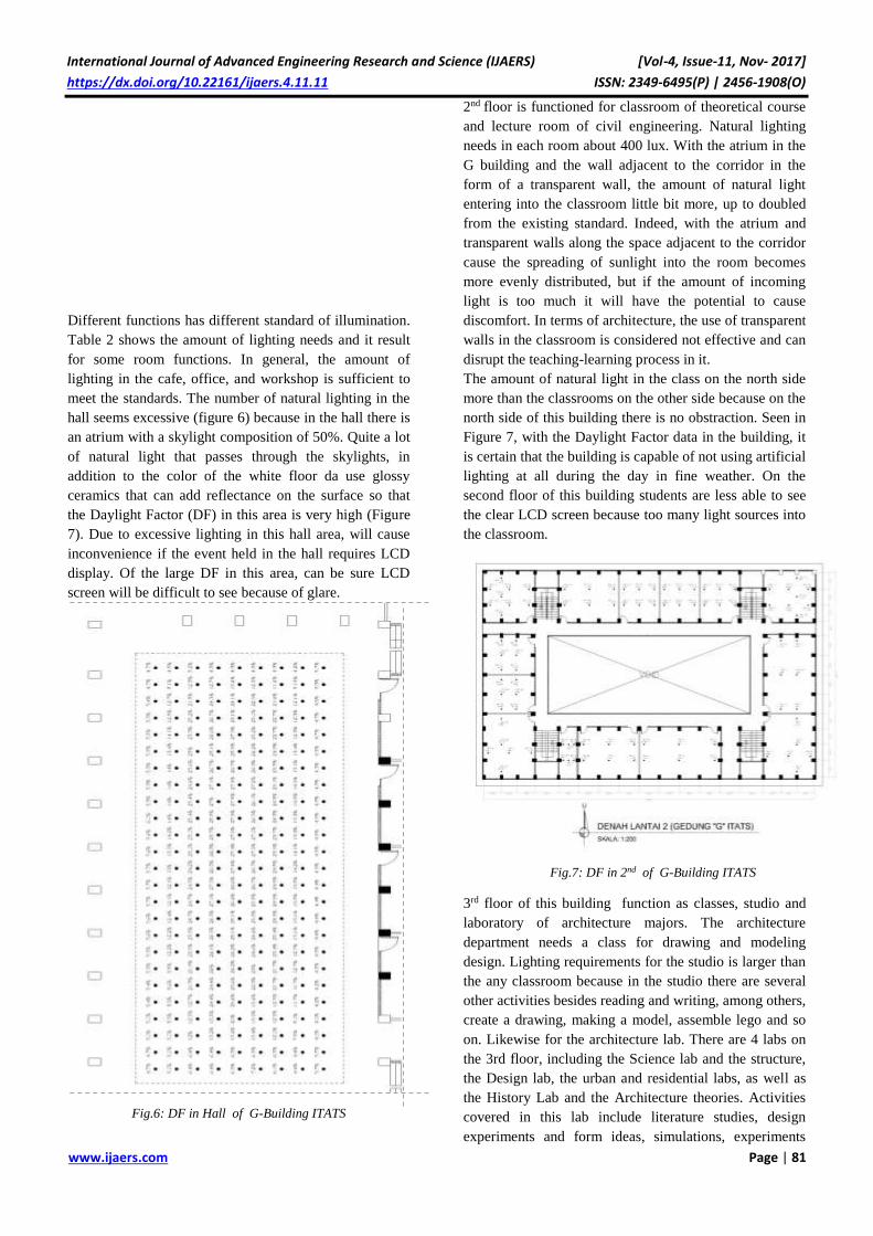
International Journal of Advanced Engineering Research and Science (IJAERS) [Vol-4, Issue-11, Nov- 2017]

https://dx.doi.org/10.22161/ijaers.4.11.11 ISSN: 2349-6495(P) | 2456-1908(O)

www.ijaers.com Page | 81

Different functions has different standard of illumination.

Table 2 shows the amount of lighting needs and it result

for some room functions. In general, the amount of

lighting in the cafe, office, and workshop is sufficient to

meet the standards. The number of natural lighting in the

hall seems excessive (figure 6) because in the hall there is

an atrium with a skylight composition of 50%. Quite a lot

of natural light that passes through the skylights, in

addition to the color of the white floor da use glossy

ceramics that can add reflectance on the surface so that

the Daylight Factor (DF) in this area is very high (Figure

7). Due to excessive lighting in this hall area, will cause

inconvenience if the event held in the hall requires LCD

display. Of the large DF in this area, can be sure LCD

screen will be difficult to see because of glare.

2nd floor is functioned for classroom of theoretical course

and lecture room of civil engineering. Natural lighting

needs in each room about 400 lux. With the atrium in the

G building and the wall adjacent to the corridor in the

form of a transparent wall, the amount of natural light

entering into the classroom little bit more, up to doubled

from the existing standard. Indeed, with the atrium and

transparent walls along the space adjacent to the corridor

cause the spreading of sunlight into the room becomes

more evenly distributed, but if the amount of incoming

light is too much it will have the potential to cause

discomfort. In terms of architecture, the use of transparent

walls in the classroom is considered not effective and can

disrupt the teaching-learning process in it.

The amount of natural light in the class on the north side

more than the classrooms on the other side because on the

north side of this building there is no obstraction. Seen in

Figure 7, with the Daylight Factor data in the building, it

is certain that the building is capable of not using artificial

lighting at all during the day in fine weather. On the

second floor of this building students are less able to see

the clear LCD screen because too many light sources into

the classroom.

3rd floor of this building function as classes, studio and

laboratory of architecture majors. The architecture

department needs a class for drawing and modeling

design. Lighting requirements for the studio is larger than

the any classroom because in the studio there are several

other activities besides reading and writing, among others,

create a drawing, making a model, assemble lego and so

on. Likewise for the architecture lab. There are 4 labs on

the 3rd floor, including the Science lab and the structure,

the Design lab, the urban and residential labs, as well as

the History Lab and the Architecture theories. Activities

covered in this lab include literature studies, design

experiments and form ideas, simulations, experiments

Fig.6: DF in Hall of G-Building ITATS

Fig.7: DF in 2nd of G-Building ITATS

International Journal of Advanced Engineering Research and Science (IJAERS) [Vol-4, Issue-11, Nov- 2017]

https://dx.doi.org/10.22161/ijaers.4.11.11 ISSN: 2349-6495(P) | 2456-1908(O)

www.ijaers.com Page | 82

using wind tunnel and helliodon. Lighting requirements

for a 900lux or DF 9% lab.

In general, the performance of lighting on the 3rd floor is

quite good and the spread is also evenly distributed

(figure 8). In DF classes and incoming studios is greater

than the standard, but the natural incoming LAB inbox is

still less than required. This is because the layout of the

room is less laid out optimally.

The 4th floor has an identical floor plan with 3rd floor.

This 4th floor room is used for classrooms, reading rooms

and studios in department of product design. Studio

product design more likely a workshop so that the need

for lighting is also greater than the studio in architecture

department. The 4th floor in overall has an average bigger

lighting than 1st-3rd floor. This is because the 4th floor

does not have any obstruction outside the room and is the

top floor so that the natural daylight distribution in the

atrium can be directly distributed in the classroom.

(Figure 9)

The natural light on the 4th floor in the workshop room is

enough to fulfill the standard and the spreading of the

light is quite evenly, for the reading room and classroom

too much natural light coming into the room so this

allows inconvenience for the users in it. Solutions for the

classroom can be overcome with curtains or blinds on the

room so that when teaching and learning process lecturers

and students can adjust the amount of natural light that

enters the room.

V. CONCLUSION

Building with 50% fenestration roof in the atrium was

able to provide a lot of natural lighting into the building

and quite effective in helping the distribution of lighting

in the perimeter space. Indeed, in some rooms amount of

natural light level is too big, but there is a solution by

installing the curtain on the window. Subsequent research

can evaluate the amount of percentage of skylight on the

atrium to make the distribution of natural lighting more

evenly and the amount of heat entering the building is not

too large.

ACKNOWLEDGEMENTS

Thanks to ristekdikti has been a sponsor of this research.

REFERENCES

[1] Yeang Ken (1996), Bioclimatic Skyscraper. London:

Artemis London Limited

[2] Baker Nick dan Koen Steemers, (2005), Energy and

Environmental in Architecture, Taylor & Francis

Group, New York

[3] Knowles, R.L. (2003), “The Solar Envelope: Its

Meaning for Energy and Buildings”, Journal of

Energy and Buildings

[4] Dian P.E. Laksmiyanti (2016), Kinerja Bentuk

Bangunan Perkantoran Bertingkat Menengah Di

Surabaya Terhadap Efisiensi Energi Pendinginan,

Jurnal IPTEK ITATS vol:20 no 1.

[5] Crawford Robert H, Czerniakowski Isabella, Fuller

Robert J (2010), A comprehensive framework for

assessing the life cycle energy of building

construction assemblies, Journal Science Direct,

Architectural Science Review 53 (2010) 288–296.

[6] Heerwagen Dean (2004), Passive and Active

Environmental Controls Informing The Schematic

Design of Building, Mc Graw Hill, New York

[7] Markus T.A, Morris E.N (1980), Buildings, Climate

and Energy, Pitman Publishing Limited, London

[8] Olgyay, V (1972). Design with Climate- Bioclimatic

approach to architectural regionalism, Princeton

University Press, New Jersey

Fig.8: DF in 3rd of G-Building ITATS

Fig.9: DF in 4th of G-Building ITATS

International Journal of Advanced Engineering Research and Science (IJAERS) [Vol-4, Issue-11, Nov- 2017]

https://dx.doi.org/10.22161/ijaers.4.11.11 ISSN: 2349-6495(P) | 2456-1908(O)

www.ijaers.com Page | 83

[9] Lenchner Norbert (2007), Heating, Cooling and

Lighting, PT. Raja Grafindo Persda, Jakarta

[10] Szokolay, S.V. (1987), Thermal Design of Buildings.

RAIA Education Division, Canberra, Australia.

International Journal of Advanced Engineering Research and Science (IJAERS) [Vol-4, Issue-11, Nov- 2017]

https://dx.doi.org/10.22161/ijaers.4.11.12 ISSN: 2349-6495(P) | 2456-1908(O)

www.ijaers.com Page | 84

Application of Cubic Spline Interpolation to Fit

the Stress-Strain Curve to SAE 1020 Steel Otávio Cardoso Duarte, Pedro Américo Almeida Magalhães Junior

Department of Mechanical Engineering, Pontifícia Universidade Católica de Minas Gerais, Brazil

Abstract —This article presents the methodology to use

cubic splines interpolation method to fit the stress-strain

curve, in the field of permanent deformation, based on

experimental data obtained on performed tests on a

standardized specimen of SAE 1020 steel hot rolled flat.

The third-order polynomial for each interval between

knots was used to fit the stress-strain curve.

Keywords— Cubic Spline, Permanent Deformation,

Curve, Interpolation, Steel.

I. INTRODUCTION

According to Vicente Chiaverini (1986), the materials

tend to deform when subjected to mechanical stresses,

and, depending on the nature of each material, their

behavior during deformation may vary. Metals can

undergo considerable permanent deformation before to

rupture. The application of cubic splines for the

construction of the strain-strain curve, in the field of

permanent deformation, through the mathematical

manipulation of data obtained in experimental tests,

allows the identification of third-order interpolator

polynomials to obtain the value of the acting axial tension

for a certain measured deformation.

The benefits are the possibility of obtaining values of the

axial tension for a given deformation, point of constraint

and better approximation of the stress-strain curve.

II. MATERIAL AND METHODOLOGY OF

THE TEST

The experimental data were obtained by tensile tests

performed on samples of specimens made of SAE 1020

hot rolled material. The tests were performed on a vertical

traction machine.

2.1 SPECIMEN USED ON EXPERIMENTAL TESTS

The specimens used in the tensile tests were prepared

according to the recommendations of ASTM E8 / E8M.

The material used was SAE 1020 hot rolled steel.

Fig. 1: Specimen Used on Experimental Tests

2.2 METHODOLOGY OF THE EXPERIMENTAL

TESTS

The tests were carried out on four identical samples of the

test specimen, in order to compare the values obtained in

the tests and to guarantee the responses of the equipment

used.

The specimens were fixed to the vertical traction machine

by means of wedge-shaped jaws, suitable to reduce

slippage during load application, which reduces errors in

data collection.

The axial tensile load was applied to the test pieces

gradually, causing the deformation of the same. The axial

tensile load was raised until fracture of each of the test

specimens used in the tests.

2.3 RESULTS OBTAINED IN THE

EXPERIMENTAL TESTS

The results obtained in the tensile tests of each of the four

test specimens are described in the table below. Seven

measuring points were taken, all within the permanent

deformation field, where the values of the axial tensile

load and its respective value of permanent deformation of

the specimen were collected.

The value of the deformation collected in the first

measurement covers the field of elastic deformation,

which was linear for all the specimens tested. As this

work aims to work only with the data of the curve of

permanent deformation, which is not linear, the data

referring to the field of elastic deformation were

suppressed.

International Journal of Advanced Engineering Research and Science (IJAERS) [Vol-4, Issue-11, Nov- 2017]

https://dx.doi.org/10.22161/ijaers.4.11.12 ISSN: 2349-6495(P) | 2456-1908(O)

www.ijaers.com Page | 85

Table. 1: Results of Experimental Tests

III. MATHEMATICAL ANALYSIS OF

RESULTS OF EXPERIMENTAL TESTS

3.1 MATHEMATICAL TREATMENT OF TEST

RESULTS

Based on the results obtained in the experimental tests, a

new the table was elaborated with the results that will be

taken as basis for the application of the interpolating

polynomials of the cubic splines. "Table 2" was

constructed by taking as reference the mean values

obtained in the experimental tests of the four specimens

of the specimen.

Table. 2: Mean values obtained in the experimental tests.

The data in Table 2 will be used to develop the

mathematical equations that will be demonstrated in the

next topic.

3.2 MATHEMATICAL TREATMENT OF TEST

RESULTS

According to Steven C. Charpa and Raymond P. Canale

(2011), the spline concept originated from a drawing

technique in which a thin, flexible strip (called a spline)

was used to draw a smooth curve through a set of points .

A smooth cubic curve results from interspersing the strip

between the pins. Thus, the name "cubic splines" was

adopted for such polynomials.

Cubic splines will be applied to determine a third-order

polynomial, for each of the intervals, of the seven

experimental measurements, in order to approximate the

strain x strain curve of the experimental results.

First, we will write the third-order polynomials for each

of the experimental data ranges.

112

13

1)( dxcxbxa=xS . x ϵ [7,44;9,30] (1)

222

23

2)( dxcxbxa=xS . x ϵ [9,30;11,16] (2)

332

33

3)( dxcxbxa=xS . x ϵ [11,16;13,02] (3)

442

43

4)( dxcxbxa=xS . x ϵ [13,02;14,88] (4)

552

53

5)( dxcxbxa=xS . x ϵ [14,88;16,74] (5)

662

63

6)( dxcxbxa=xS . x ϵ [16,74;18,60] (6)

Applying the condition that the function values must be

equal at the interior knots, and the first and last functions

must pass through the end points, we have the following

equations:

S(7,44)=411,83.a1+55,35.b1+7,44.c1+d1=38,76 (7)

S(9,30)=804,36.a1+86,49.b1+9,30.c1+d1=45,56 (8)

S(9,30)=804,36.a2+86,49.b2+9,30.c2+d2=45,56 (9)

S(11,16)=1389,93.a2+124,55.b2+11,16.c2+d2=49,80 (10)

S(11,16)=1389,93.a3+124,55.b3+11,16.c3+d3=49,80 (11)

S(13,02)=2207,16.a3+169,52.b3+13,02.c3+d3=51,89 (12)

S(13,02)=2207,16.a4+169,52.b4+13,02.c4+d4=51,89 (13)

S(14,88)=3294,65.a4+221,41.b4+14,88.c4+d4=52,88 (14)

S(14,88)=3294,65.a5+221,41.b5+14,88.c5+d5=52,88 (15)

S(16,74)=4691,01.a5+280,23.b5+16,74.c5+d5=52,92 (16)

S(16,74)=4691,01.a6+280,23.b6+16,74.c6+d6=52,92 (17)

S(18,60)=6434,86.a6+345,96.b6+18,60.c6+d6=51,68 (18)

Applying the condition that the first derivatives at the

interior knots must be equal, we have the following

equations:

259,47.a1+18,60.b1+c1 =259,47.a2+18,60.b2+c2 (19)

373,64.a2+22,32.b2+c2 =373,64.a3+22,32.b3+c3 (20)

508,56.a3+26,04.b3+c3 =508,56.a4+26,04.b4+c4 (21)

664,24.a4+29,76.b4+c4 =664,24.a5+29,76.b5+c5 (22)

840,68.a5+33,48.b5+c5 =840,68.a6+33,48.b6+c6 (23)

Applying the condition that the second derivatives at the

interior knots must be equal, we have the following

equations:

55,80.a1+2.b1 =55,80.a2+2.b2 (24)

66,96.a2+2.b2 =66,96.a3+2.b3 (25)

78,12.a3+2.b3 =78,12.a4+2.b4 (26)

89,28.a4+2.b4 =89,28.a5+2.b5 (27)

100,44.a5+2.b5 = 100,44.a6+2.b6 (28)

Applying the condition that the second derivatives at the

end knots are zero, we have the following equations:

02.b+44,64.a 11 (29)

02.b+.a60,111 66 (30)

International Journal of Advanced Engineering Research and Science (IJAERS) [Vol-4, Issue-11, Nov- 2017]

https://dx.doi.org/10.22161/ijaers.4.11.12 ISSN: 2349-6495(P) | 2456-1908(O)

www.ijaers.com Page | 86

Solving the linear system, from equation 7 to equation 30,

with their respective twenty-four unknowns, the

following values were obtained.

a1 = -0,05497, b1 =1,22701, c1= -5,28285 e d1 =32,78479;

a2 = -0,03342, b2 =0,62565, c2 =0,30979 e d2 = 15,44759;

a3=0,07327, b3= -2,94646, c3=40,17451 e d3= -133,42537;

a4 = -0,00696, b4=0,18739, c4 = -0,62827 e d4 = 43,65871;

a5 = -0,02213, b5 =0,86487, c5= -10,70909 e d5=93,65957;

a6 =0,04421, b6 = -2,46692, c6=45,06517 e d6= -217,5607.

In this way, we can write the polynomials that

approximate the value of the acting axial stress as a

function of the deformation measured in the experimental

tests, for each of the intervals between the measurements.

S(x)= -0,05497.x3 + 1,22701.x2 - 5,28285.x + 32,78479;

if x ϵ [7,44;9,30]

S(x)= -0,03342.x3 + 0,62565.x2 + 0,30979.x + 15,44759;

if x ϵ [9,30;11,16]

S(x) = 0,07327.x3 - 2,94646.x2 + 40,17451.x - 133,42537;

if x ϵ [11,16;13,02]

S(x)= - 0,00696.x3 + 0,18739.x2 - 0,62827.x +43,65871;

if x ϵ [13,02;14,88]

S(x)= -0,02213.x3 + 0,86487.x2 - 10,70909.x +93,65957;

if x ϵ [14,88;16,74]

S(x) = 0,04421.x3 - 2,46692.x2 + 45,06517.x - 217,56079;

if x ϵ [16,74;18,60]

3.3 APPROXIMATION OF THE STRESS-STRAIN

CURVE WITH THE USE OF THE CUBIC

SPLINES

The cubic splines that approximate the stress values for

the deformations evidenced in the experimental tests,

obtained through the mathematical methods demonstrated

in topic 2.2, were used to construct the strain-strain curve,

as can be seen in Fig. 2.

The curve was constructed with the application of the

cubic splines in the numerical calculation software VCN.

Fig. 2: Stress x strain curve obtained through the cubic

spline polynomials

ACKNOWLEDGEMENTS

I thank the staff of the mechanical testing laboratory of

the Pontifica Universidade Católica de Minas Gerais, for

the help they gave me in the execution of the traction

tests, and to Professor Dr. Pedro Américo Almeida

Magalhães Junior, for the technical support in the

elaboration of this article.

REFERENCES

[1] Chapra, Steven C., Canale, Raymond P., 2011.

Métodos Numéricos para Engenharia. McGraw-Hill.

[2] Chiaverini, Vicente., 1986. Tecnologia Mecânica:

Estruturas e Propriedades das Ligas Metálicas.

McGraw-Hill.

International Journal of Advanced Engineering Research and Science (IJAERS) [Vol-4, Issue-11, Nov- 2017]

https://dx.doi.org/10.22161/ijaers.4.11.13 ISSN: 2349-6495(P) | 2456-1908(O)

www.ijaers.com Page | 87

Tensile Test: Comparison Experimental,

Analytical and Numerical Methods Tatiana Lima Andrade, Pedro Américo Almeida Magalhães Júnior, Wagner Andrade de

Paula

Department of Mechanical, Pontifical Catholich University of Minas Gerais, BRAZIL

Abstract—The objective of this work is to study and

analyze the stress-strain curves obtainedthrough the

experimental tensile test and the comparison of thedata

obtainedwith the analytical and numerical methods. For

the development of the analytical method, we proposed

equations for the stress-strain curve of the material, using

MS-EXCEL 2016. For the numerical method, a modeling

of the test specimen was elaborated using the ANSYS

Workbench® version 16 software. The steel selected for

the studies was ABNT 1020.

Keywords—Hooke’s Law, Plastic-strain, Tensile test.

I. INTRODUCTION

Tensile test was used for evaluating the mechanical

properties of material and the plastic strain modify this

properites.

Use tensile test for determinate the final of plastic phase.

([2])

The state of tension in which plastic deformation occurs

dependent on the degree of current plastic deformation

and this phenomenon is called hardening. ([1])

II. METHODOLOGY

2.1 Experimental Methodology

The methodology based on experimental analysis using

ABNT 1020 material specimen.

After the test will be collected the data obtained and

generated the stress-strain curves of the engineering and

actual deformation of the test.

The data obtained of the test will shown in Table 1.

Table1:TensileTest Data

Data Value

Maximum Stress [MPa] 546.60

Area [mm2] 63.62

Initial length [mm] 55.50

Final length [mm] 73.00

Initial diameter [mm] 9.00

Final diameter [mm] 5.10

With the achievement tensile stress, the stress-strain curve

constructed, as shown in Figures 1 below.

Fig. 1: Experimental curve

2.2 Analytical Methodology

In the analytical method, it proposed the determination of

a curve that approached the stress strain curve obtained

from the tensile test.

To determination the curves describing the behavior of

the material, divided the curve experimental curve

through pre-established intervals.

Four different equations has developed to divide into the

following phases of the behavior of the material: elastic

phase, beginning of the flow stage, ending of elastoplastic

transition and plastic phase.

The selected interval of the curves has approximated by

log, exponential or polynomial tendency curves.Thus,

equations has developed that approached the maximum of

the real curve of the tensile test.

2.3 Elastic Phase

The proposed curve for the elastic phase of the material

uses Hooke's law, (1) and shown inFig. 2.

𝜎 = 𝐸. 𝜀𝜎 < 𝜎𝑒𝑠𝑐 (1)

σ = tensile stress [MPa]

ɛ = strain [MPa]

E = elastic modulus

International Journal of Advanced Engineering Research and Science (IJAERS) [Vol-4, Issue-11, Nov- 2017]

https://dx.doi.org/10.22161/ijaers.4.11.13 ISSN: 2349-6495(P) | 2456-1908(O)

www.ijaers.com Page | 88

Fig. 2: Elastic phase curve

2.4 Beginning of the flow stage

The curve proposed for the beginning of the flow

stageuses, (2) with the constants values of A and b shown

below. The curves shown in Fig. 3.

𝜎 = 𝐴. 𝑒𝑏.𝜀 𝜀 > 𝜀𝑒𝑠𝑐 (2)

σ = tensile stress [MPa] ɛ = strain [MPa]

A = 432.248 b = 0.001

Fig. 3: Beginning of the flow stage

2.5 Ending of elastoplastic transition

The curve proposed for the ending of elastoplastic

transition considers, (3) with the constants values of C

and d shown below. The curves shown in Fig. 4.

𝜎 = 𝐶. 𝜀𝑑 + 𝐹. 𝜀 + 𝐺 𝜀 < 𝜀𝑒𝑝 (3)

σ = tensile stress [MPa] ɛ = strain [MPa]

c = -6.5945 d = 2

F =163.39 G = -485.62

Fig. 4: Ending of elastoplastic transition

2.6 Plastic Phase

The curve proposed for the plastic phase uses, (4) with the

constants values of H and K shown below. The curves

shown in Fig. 5.

𝜎 = 𝐻. 𝑙𝑛𝜀 + 𝐾 𝜀 > 𝜀𝑒𝑝 (4)

σ = tensile stress [MPa] ɛ = strain [MPa]

H = 160.674 K = 140.04

Fig. 5: Plastic phase

2.7 Developed curve using the proposed equations

For development of proposed curve has been used the

equations 3 to 6. The Fig. 6 shown the proposed curve of

performed tensile test.

Fig. 6: Proposed curve

III. COMPARISON OF EXPERIMENTAL AND

ANALYTICAL METHODS CURVES

The Fig. 7 shown the comparison of experimental and

analytical methods curves of the ABNT 1020 material.

International Journal of Advanced Engineering Research and Science (IJAERS) [Vol-4, Issue-11, Nov- 2017]

https://dx.doi.org/10.22161/ijaers.4.11.13 ISSN: 2349-6495(P) | 2456-1908(O)

www.ijaers.com Page | 89

Fig. 7: Comparison curves

IV. NUMERICAL METHODOLOGY

The test specimen of ABNT 1020 material modeled in the

AutoCad 16 and imported to ANSYS 16, in the

Mechanical module a mesh has defined for it and its

restrictions and loads were created. A fixed support has

created at the base of the specimen and load has applied

to the top of the specimen, as seen in Figs. 8 and 9.

Fig. 8: Test specimen mesh

Fig. 9: Test specimen constrain

The displacement are show in Fig. 10 and tensions

obtained are shows in Fig.11.

Fig. 10: Test specimen displacement

Fig. 11: Test specimen stress

The obtained curve through the numerical simulation

shown in Fig. 12.

Fig. 12: Numerical curve

A curve of Fig. 13was designed in MS-Excel. The curve

were created stress as a function of time, but it can be

observed that the behavior of the curve is similar to those

International Journal of Advanced Engineering Research and Science (IJAERS) [Vol-4, Issue-11, Nov- 2017]

https://dx.doi.org/10.22161/ijaers.4.11.13 ISSN: 2349-6495(P) | 2456-1908(O)

www.ijaers.com Page | 90

found in the experimental and analytical analyzes,

because it presents an elastic phase, an elastoplastic

transition and the plastic phase.

Fig. 13: Numerical curve – MS-Excel

V. CONCLUSION

The results were as expected. The specimen rupture

occurs approximately 35 mm, as shown in Fig. 11.

The tensile test was of great importance to have a

practical knowledge of the engineering data used in

mechanical designs.

By comparing the experimental, analytical and numerical

methods, one can note the importance of each one of them

and how important it is to have an idea of the behavior of

the material for the use of a numerical method in a safe

and reliable way.

The results were as expected. The specimen rupture

occurs approximately 35 mm, as shown in Fig. 11.

The advantage of this study is the confidence obtained in

the execution of the proposed methodology, since the

results obtained are very close to the experimental test.

ACKNOWLEDGEMENTS

The authors thank the support of the Pontifícia

Universidade Católica de Minas Gerais – PUCMINAS-

“Pontifical Catholic University of Minas Gerais”, the

Conselho Nacional de Desenvolvimento Científico e

Tecnologico-CNPq-“National Counsel of technological

and scientific Development”, the Fundação de Amparo a

Pesquisa de Minas Gerais-FAPEMIG-“Foundation for

Research Support of Minas Gerais”.

REFERENCES

[1] EVANGELISTA, Sérgio Henrique,2000. Diagrama

de limite de conformaçãoaplicados a

análiseporelementosfinitos de um processo de

estampagememchapasmetálicas. 135f. Dissertação

(Mestrado) – Universidade de São Paulo Escola de

Engenharia de São Carlos,

MestradoemEngenhariaMecânica, São Paulo, 2000.

[2] RISITANO, A. et al, 2017. Fatigue assessment by

energy approach during tensile tests on AISI 304

steel. Fracture and Structural Integrity, [S.l.], n. 39, p.

Pages 201-215, dec. 2016. ISSN 19718993.

Available at:

<http://www.fracturae.com/index.php/fis/article/view

/IGF-ESIS.39.20/1858>. Date accessed: 30 set 2017.

doi:http://dx.doi.org/10.3221/IGF-ESIS.39.20.

[3] K. Polaiah, Hemalatha. Naidu, P. Satheesh Kumar

(2017).Friction Stir Welding of Similar Metals by

Taguchi Optimization Technique -A Review.

International Journal of Advanced Engineering,

Management and Science(ISSN: 2454-1311),3(10),

0991-0994. http://dx.doi.org/10.24001/ijaems.3.10.3

[4] B.S. Krishnamurthy, R. Balamuralikrishnan,

Mohammed Shakil (2017).An Experimental Work on

Alkaline Resistance Glass Fiber Reinforced concrete.

International Journal of Advanced Engineering,

Management and Science(ISSN: 2454-1311),3(7),

730-737. http://dx.doi.org/10.24001/ijaems.3.7.4

International Journal of Advanced Engineering Research and Science (IJAERS) [Vol-4, Issue-11, Nov- 2017]

https://dx.doi.org/10.22161/ijaers.4.11.14 ISSN: 2349-6495(P) | 2456-1908(O)

www.ijaers.com Page | 91

Review on Exhaust Heat Recovery Systems in

Diesel Engine Mohamed Shedid, Moses Sashi Kumar

Mechanical Engineering Department, SUR University College, Sur 411, Oman

Abstract— Exhaust heat recovery system converts the

thermal losses in the exhaust zone in engines into energy

for work. This technology also reduces exhaust emission

from engines. This review paper extends the classification

of various methodologies on EHR in diesel engine. In

spite of their indigenous benefit for various technologies,

it has some limitation over applications to different

context. From the current researches the variation in

usage of exhaust heat from the diesel engine is evaluated

and compared to find which methodology is suitable to

attain high efficiency in thermal recovery for power

generation. Finally a novel method of an EHR system is

proposed to increase high percentage of heat recovery

from the exhaust gas in diesel engines.

Keywords— Exhaust heat recovery system, diesel

engine.

I. INTRODUCTION

Diesel engines are used in varied applications and it is

also a part of a widely networked global system defined

by the concepts of ‘‘resources’’ and ‘‘environmental

pollution’’. It is based purely on energy and economics

aimed at minimizing the heat losses that fails to satisfy

present day demands specified by the ecological

imperative according to which energy and material must

always be converted with maximum efficiency while

minimally polluting the environment [1]. Just like

gasoline engines, diesel engines are, in principle, energy

converters that convert chemically bound fuel energy into

mechanical energy (effective work) by supplying the heat

released by combustion in an engine to a thermodynamic

cycle. The heat released from the engine can be recovered

to appropriate work. Researchers confirm that more than

30–40% of fuel energy gets wasted from the exhaust and

just 12–25% of the fuel energy converts to useful work

[2,3]. On the other aspect the toxic emissions from the

exhaust gases leads to public awareness of the finiteness

of fossil fuel. It has receded into the background

somewhat after being raised in the 1970s; the impact of

pollutant and CO2 input into the earth’s atmosphere is

again making the need for a longer-range environmentally

compatible energy policy with concrete goals evident to

suppress the greenhouse effect. For a better future, both

challenges conserving resources and protecting the

environment would require an approach that endeavors to

take full advantage of the ample potentials to save energy

and additionally intensify the utilization of inexhaustible

energy sources. These challenges will necessitate the

research on various waste heat recovery schemes that

accumulate on diesel engine through various forms for

conserving the primary energy of the fuel and protecting

the environment.

Exhaust heat recovery system

Exhaust heat recovery system is an energy recovery heat

exchanging process that recovers heat with high potential

energy in sources like diesel engine for improving its

efficiency. In the present scenario there is a substantial

demand of energy for global applications, so the usage of

conventional fuels and its toxic exhaust gases will

increase the effect of global warming. With the aspect to

dwindle the usage of fossil fuels many researchers

attempt to recover the waste heat from diesel engines.

Various forms of heat can be categorized from engines on

their origin

Heat losses from the exhaust gas through exhaust

pipeline,

Waste heat produced as cooling energy to protect

engine seize,

Waste heat from intercooling to boost engine power

and net efficiency,

Waste heat convected through the engine surface.

During combustion cycle in engines the exhaust gases are

dissipated through gas exchange process at a range of

300-500°C. Other sources of waste heat from engine will

be transferred to the surroundings with the aid of coolant.

Heat transfer occurs through the coolant medium (air,

water or oil) at various points of engine to recover its

complex issues. The cooling energy is transferred through

heat exchangers. In case of the exhaust gas loaded with

particulate matter and soot particulates is more critical in

heat transfer through HXs. Aerated heat from the under

hood parts usually transfer heat through radiation and

convection or heat pump which works on thermal

absorption cycle. To implement the heat recovery for

different temperature operating conditions in engines,

International Journal of Advanced Engineering Research and Science (IJAERS) [Vol-4, Issue-11, Nov- 2017]

https://dx.doi.org/10.22161/ijaers.4.11.14 ISSN: 2349-6495(P) | 2456-1908(O)

www.ijaers.com Page | 92

various technologies has been proposed by many

researchers. In this paper, a short review of the

technologies for heat recovery from engines is presented.

Review on EHR systems

Thermo electric generators

Thermoelectric generators (TEG) or See beck generators

are devices, which directly convert waste heat energy into

electrical energy. These devices work on See beck effect,

which was discovered by Thomas Johann See beck in

1821 [4]. Recently, for increasing the efficiency of these

devices, semiconductor p–n junctions were added (Fig.

1)that are made up of new materials such as Bi-Te

(bismuth telluride), CeFeSb (skutterudite), Zn-Be (zinc–

beryllium), Si-Ge (silicon–germanium), Sn-Te (tin

telluride) and new nano-crystalline or nanowire

thermoelectric which increase their efficiency to around

5–8%. Although TEG devices have many advantages

such as clean energy, without sound, without movable

component and lesser maintenance costs, they are

however only economical when used at high temperatures

(4200 1C) and when only small amounts of the power (a

few mill watts) are needed. TEG's advantages motivated

many of the researchers to use it in automobile waste heat

recoveries which can be seen in [5]. For instance, Karri et

al. [6] studied two cases of exhaust waste heat recovery

using TEGs. Also, Zhang and Chau [7] reported that

using TEG has low effect on engine performance and it

can improve the engine power up to 17.9%due to their

smaller size of energy absorbing ratio.

Fig.1. Detailed view of p-n junction semiconductor device

In this work, the heat exchanger connected with TEGs for

recovering waste heat from an automotive channel is

analyzed. As per the assention between the infrared

experimental results and the CFD simulation, a brass heat

exchanger with accordion shape and surface territory (660

mm 305 mm) is chosen to form the hot side.It can reduce

the thermal resistance between the exchanger and the

TEMs and obtain a relatively high surface temperature

and uniform temperature distribution to improve the

efficiency of the TEG as shown in fig.2.The current study

focuses on the structural optimization of the heat

exchanger and the coolant system to improve the

efficiency of the vehicular exhaust gas heat. In the later

study, the way of the simulation modeling and the

infrared experimental verification that has been

introduced in this article needs to be combined with the

heat transfer theory, to make further structural design and

optimization to improve the overall exhaust heat

utilization [8].

Fig.2: Schematic of automotive exhaust based TEG

Organic Rankine Cycle

Among these cycles, Organic Rankine Cycle (ORC) can

be introduced as the most efficient cycle for low

temperature sources such as engine exhaust. Simple ORC

is contains boiler, expander, condenser, pump and

working fluid [9]. Many works are performed in this field

and complete reviews of them are presented by Sprouse et

al.[10] and Wang et al. [11]. Most of these works are

based on the effect of working fluid type on the ORC

performance. The different types of working fluids are

wet, dry and isentropic fluids with their T–S diagram

slopes being positive, negative and infinite. Chen et al.

[12] by comparing 35 kinds of working fluids reached to

the fact that suitable working fluid depends on the

operating condition and a working fluid does not have

maximum efficiency at all conditions. Dai et al. [13]

mentioned that organic working fluids are more suitable

for low temperature sources such as engine exhaust from

the knowledge that wet fluids are never recommended for

ORC due to the interaction between fluid particles and

turbine blades. With a complicated system, Teng and

Regner[14] exploited waste heat from the EGR system of

a class-8 truck diesel engine to operate a supercritical RC

with R245fa as working fluid, as demonstrated in Fig. 9.

The fluid was superheated upstream of the expander,

which was coaxially assembled with the alternator. The

system achieved a 15.8% Rankine efficiency, which could

International Journal of Advanced Engineering Research and Science (IJAERS) [Vol-4, Issue-11, Nov- 2017]

https://dx.doi.org/10.22161/ijaers.4.11.14 ISSN: 2349-6495(P) | 2456-1908(O)

www.ijaers.com Page | 93

reach to 25.5% with ethanol as a substitute fluid. The

composite fuel savings over the ESC 13-mode test cycle

was up to 5%.

Fig.3: ARC system for waste heat recovery from diesel

engine

Five stroke cycle

The concept of five-stroke engine, invented by Schmitz

[15], does not reduce compression but increases

expansion. The 5-stroke engine is a three-cylinder in

which two cylinders perform a four-stroke cycle and

alternatively a second expansion of the burnt gases is

performed in the third cylinder. Turbocharger is adopted

to deliver the boost pressure and the system is controlled

by an innovative system called smart waste gate. It

consist of variable valve timing of the two valves of the

low pressure cylinder. [16].

Fig.4: Architecture of the 5-stroke engine showing the

valves location and the smart waste gate

Six stroke cycle

The six-stroke engine is a type of internal combustion

engine based on the four-stroke engine but with additional

complexity intended to make it more efficient and reduce

emissions. Three types of six-stroke engines have been

developed since the 1890s [17], but in one of them

proposed by Conklin and Szybist [18], the engine

captures the heat lost from the four-stroke diesel engine

and uses it to generate an additional power without more

fuel consumption. A schematic of the operation of this

engine is shown in Fig. 3. As seen, there are two power

strokes: one with fuel, the other with water injection by

using the waste heat of burned gases in the previous

stroke. Water injection is occurred after compressing the

burned gases from first stroke when the crank shaft angle

is 720°. Mean effective pressure (MEP) of these engines

will be increased by increasing the injected water amount.

The main advantages of this engine is reducing the

emissions and using from two main waste heat sources

because injected water can be preheated by using an

exhaust heat exchanger.

Fig.5: Six stroke engine cycle

Turbo charging

Dr. Alferd J. Buchi proposed the first idea of

turbochargers in 1915, which he developed it on a diesel

engine. Actually, a turbocharger is a supercharger driven

with exhaust gases energy and increases the engine power

by compressing the inlet air to engine. Fig. 4 shows a

turbocharger with its appurtenances. A turbocharged

engine is more powerful and efficient than a naturally

aspirated engine because the turbine forces more air and

proportionately more fuel into the combustion chamber

than atmospheric pressure alone, but it has some

shortcomings. Turbo- lag i.e., (hesitation or transient

response) during low speed acceleration and major

concerns with heated bearings are two main shortcomings

in turbochargers which are approximately solved by using

two stages turbochargers and variable geometry turbines

(VGT) [19]. Another concern in turbochargers is

increasing the intake air temperature due to its pressure

increase. The warmer intake air has the less density and

the less oxygen is available for the combustion event

which reduces volumetric efficiency, it also leads to

engine knock or detonation known as a destructive factor

in engines. So, turbocharger units often use an intercooler

(also known as a charge air cooler) to cool down the

intake air as shown in Fig. 4. Recently, a novel exhaust

steam recovery system (steam turbocharging) is presented

by Fu et al [20]. They set a Rankine steam cycle system

coupled on engine exhaust pipe, which utilizes the

exhaust energy of engine in order to generate steam and

International Journal of Advanced Engineering Research and Science (IJAERS) [Vol-4, Issue-11, Nov- 2017]

https://dx.doi.org/10.22161/ijaers.4.11.14 ISSN: 2349-6495(P) | 2456-1908(O)

www.ijaers.com Page | 94

then drive the turbine. Their results show that IC engine

power can theoretically be improved by 7.2% at most and

thermal efficiencies can be raised up to 2 percent or more.

EGR system

Recirculation of the exhaust gases into cylinder or EGR is

one of the efficient methods to decrease the NOx level.

EGR can be applied internally or externally in the

engines. EGR is widely used in both gasoline and diesel

engines reviewed by Wei et al. [21] and Zheng et al. [22],

respectively. In a diesel engine, the exhaust gas replaces

some of the excess oxygen in the pre-combustion mixture.

Since NOx is formed primarily when a mixture of

nitrogen and oxygen is injected into high temperature

circumstances, the lower temperatures of combustion

chamber caused by EGR reduce the amount of the NOx.

EGR cannot improve the combustion irreversibility, but it

can be assumed as a technique for using the heat of

burned gases in the cylinder for another time [23].

Furthermore in modern diesel engines, the EGR gases are

cooled with a heat exchanger in order to enter a greater

mass of recirculated gases.

Pneumatic power system

Pneumatic hybridization of ICEs was first discussed in

the 1990s [24,25]. HPPS generally consists of an ICE, an

air compressor, a pressure tank, and a high-efficiency

turbine. A concept schematic setup of HPPS is shown in

Figure 4. The main working principle of pneumatic

hybridization engines is to recover energy from a braking

phase or from a combustion phase by pumping the

exhaust gas or the pressurized air into the air tank, and

then the air tank can then be restored to start the engine or

charge the engine during the strong transient accelerations

or short-term high-power output period. An advantage of

the pneumatic hybridization engine is that the pressurized

air can be pumped into the combustion chamber to

overcome the turbo-lag problem during the speedup

period of the turbocharger, which can maximize the

performance of the turbocharger. Pneumatic hybridization

engines also offer improved fuel economy and reduced

emissions. Compared with a conventional diesel vehicle

for the drive cycles of NEDC, UDDS, HWFET, and

JAPAN10-15, Chen and Xu believed that the parallel

pneumatic hybrid vehicle could decrease emissions by

58.84% (NEDC), 38.76% (UDDS), 14.54% 4(HWFET),

and 66.59% (JAPAN10-15), and save energy by 13.12%,

14.06%, 16.27%, and 28.06%, respectively [26].

According to simulation results, the overall efficiency of

HPPS can be expected to increase by approximately 20%

[27]. Donitz et al. even concluded that, the combination

of engine downsizing and pneumatic hybridization yields

a fuel consumption reduction of up to 34% for the

MVEG-95 drive cycle [28]. However, the merging

problem between the high- pressure flow in the air tank

and the high-temperature exhaust gas in the ICE must also

be considered. Huang et al. [29] studied the effects of the

level of compressed air pressure (Pair) and the contraction

of the cross-section area at the merging position on the

flow energy merger and found that exhaust gas energy

recycling efficiency and merger flow energy are

significantly dependent on the optimum adjustment of the

cross-section area for changes in Pair.

Thermal distillation system

Fig.6: Schematic view of hybrid pneumatic power system

The aim of this work is to utilize the heat energy wasted

in exhaust gas of an internal combustion engine of low

capacity for desalination using a submerged horizontal

tube straight pass evaporator and a condensing unit,

without the aid of any external energy. A horizontal tube

straight pass evaporator and water-cooled condenser for

condensing the evaporated steam were designed and

fabricated. The experiments were conducted in a 5 hp

diesel engine to analyze the performance of the

submerged horizontal tube straight pass evaporator

(SHTE) under various load conditions. It is evident that

3.0 l/h of saline water can be desalinated from the engine

exhaust gas without affecting the performance of the

engine. More over nearly 24 litre of water is heated, up to

60 °C in the condenser unit. By utilizing the heat energy

in condenser water in addition to waste exhaust gas heat

energy the overall efficiency of the system is enhanced

and thermal pollution is also reduced considerably [30].

Combined air cycle power generator

A combined air cycle is designed for

International Journal of Advanced Engineering Research and Science (IJAERS) [Vol-4, Issue-11, Nov- 2017]

https://dx.doi.org/10.22161/ijaers.4.11.14 ISSN: 2349-6495(P) | 2456-1908(O)

www.ijaers.com Page | 95

Fig.7: Circuit view of thermal distillation from EHR

system

Internal combustion (IC) engine supercharging. The setup

consists of IC engine working cycle and bottom cycle of

waste heat recovery (WHR). IC engine exhaust gas is

used to run the bottom cycle and its power used to drive

the gas compressor. Numerical calculation were

performed for both the heat transfer and thermodynamic

processes of combined air cycle for different cycle

parameters and IC engine operating conditions. Results

show that the cycle efficiency and exhaust gas energy

recovery efficiency depend largely on the working

pressure and their maximum values appear at the working

pressure of 0.35 MPaand 0.2 MPa respectively. This

approach can make the fuel utilization efficiency of IC

engine increase by 8.9% points and 4.1% points at most

respectively compared with the naturally aspirated (NA)

engine and turbocharging engine due to the reduction of

exhaust gas pressure. [31]. Gao et al. [32]have proposed a

WHR system where a high speed turbocharged diesel

engine acts as the topper of a combined cycle with

exhaust gases used for a bottoming Rankine cycle. And

the result shows that heat recovery system can increase

the engine power output by 12%, when diesel engine

operates at 80 kW/2590 rpm.

Fig.8: Schematic view of combined air cycle EHR system

Thermal storage system

Schatz [33] introduced the concept of a heat battery to

store the engine waste heat using a PCM. They reported

that the possible way of recovering the waste heat from

the IC engine coolant and storing the heat in a PCM heat

battery through experiments.This stored heat is used

during engine cold start condition by transferring heat

from PCM to the engine coolant, which ensures the

engine to attain operating temperature substantially faster.

The energy available in the exit stream of many energy

conversion devices goes as waste, if not utilized properly.

The exhaust gas from an internal combustion engine

carries away about 30% of the heat energy of combustion.

The major technical constraint that prevents successful

implementation of waste heat recovery is due to its

intermittent and time mismatched demand and availability

of energy. In the present work a shell and finned tube heat

exchanger combined with an IC engine setup to is used to

recover the heat from the exhaust gas and a thermal

energy storage tank used to store the excess energy

available is investigated in detail. A combined sensible

and latent heat storage system is designed, fabricated and

tested for thermal energy storage using cylindrical phase

change material (PCM) capsules. The performance of the

engine with and without heat exchanger is evaluated.

Results shows that nearly 10–15% of fuel power is stored

as heat in the combined thermal storage system. The

performance parameters pertaining to the heat exchanger

and the storage tank such as amount of heat recovered,

heat lost, charging rate, charging efficiency and

percentage energy saved are evaluated and reported in

this paper [34].

Fig.9: Layout setup of thermal storage PCM tank

Proposed methodology

The proposed methodology is an integration of

thermoelectric generator with shell and tube heat

exchangers for exhaust heat recovery system. The model

consists of a shell and tube heat exchanger with a

modified slot for TEG device i.e. (current conducting

medium) placed on the middle of heat exchanger. The

surface of the p-n junction device will be in contact with

the thermo-electric fluid (ionic fluid) acts as a carrier

medium. This absorbs the heat losses from the exhaust

gas produced in the diesel engine and the cold fluid from

the radiator outcome. With this integration effect, we can

achieve a greater efficiency in HER system. The typical

circuit of the proposed heat exchanger is shown in Fig.10.

International Journal of Advanced Engineering Research and Science (IJAERS) [Vol-4, Issue-11, Nov- 2017]

https://dx.doi.org/10.22161/ijaers.4.11.14 ISSN: 2349-6495(P) | 2456-1908(O)

www.ijaers.com Page | 96

Fig.10: Layout of proposed pumping heat recovery

system

II. CONCLUSION

In this paper, a short review of heat recovery technologies

in engines and heat exchangers has been presented. It

seems that in most of these technologies (ORC, TEG,

EGR, and turbo- charging), heat exchangers have an

important role to transfer heat for recovering process, so a

suitable design for heat exchanger should be applied in

accordance with this fact that heat transfer increases when

pressure drop is in the allowable limit. Some experimental

and numerical researches about various heat exchangers

designs existed in the literature which all of them have

been reviewed here. It can be concluded that using fins is

more applicable and appropriate than foams and porous

materials due to the lower pressure drop and higher heat

transfer rate. Also, it seems that other methods for

increasing the heat transfer such as vortex generators,

nanofluids, using the PCM as heat storage source, etc., in

addition to lower TEGs in downstream of HEX, design

parallel HEXs or HEX with one inlet and two outlets,

selecting the best solid materials, TEGs material and

working fluids can enhance the exhaust heat recovery and

save the fuel costs for future works.

REFERENCES

[1] Klaus Mollenhauer, Helmut Tschoeke.Handbook of

Diesel Engines.Springer Publications.

[2] Saidur R Rahim NA, Ping HW JahirulMI, Mekhilef

S Masjuki HH. Energy and emission analysis for

industrial motors in Malaysia. Energy Policy

2009;37 (9):3650–8.

[3] Hasanuzzaman M Rahim NA, Saidur R Kazi SN.

Energy savings and emissions reductions for

rewinding and replacement of industrial motor.

Energy 2011;36(1):233–40.

[4] Riffat SB, Ma X. Thermoelectrics: a review of

present and potential applications. Appl Thermal

Eng 2003;23(8):913–35.

[5] Saidur R, Rezaei M, Muzammil WK, Hassan MH,

Paria S, Hasanuzzaman M. Technologies to recover

exhaust heat from internal combustion engines.

Renew Sustain Energy Rev 2012;16:5649–59.

[6] Karri MA, Thacher EF, Helenbrook BT. Exhaust

energy conversion by thermoelectric generator: two

case studies. Energy Convers Manage 2011;52(3):

1596–611.

[7] Zhang X, Chau KT. An automobile thermoelectric–

photovoltaic hybrid energy system using maximum

power point tracking. Energy Convers Manage

2011;52(1):641–7.

[8] C.Q. Su, W.S. Wang, X. Liu, Y.D. Deng. Simulation

and experimental study on thermal optimization of

the heat exchanger for automotive exhaust-based

thermoelectric generators.Case Studies in Thermal

Engineering 2014; 4: 85–91

[9] Duparchy A Leduc P, Bourhis G Ternel C. Heat

recovery for next generation of hybrid vehicles:

simulation and design of a Rankine cycle system.

3World Electric Vehicle 2009.

[10] SprouseIII C, Depcik C. Review of Organic Rankine

Cycles for internal combustion engine exhaust waste

heat recovery. Appl Thermal Eng 2013;51: 711–22.

[11] WangTianyou, Zhang Yajun, PengZhijun,

ShuGequn. A review of researches on thermal

exhaust heat recovery with Rankine cycle. Renew

Sustain Energy Rev 2011;15:2862–71.

[12] Chen H, Goswami DY, Stefanakos EK. A review of

thermodynamic cycle and working fluids for the

conversion of low-grade heat. Renew Sustain

Energy Rev 2010;14:3059–67.

[13] Dai YP, Wang JF, Gao L. Parametric optimization

and comparative study of Organic Rankine Cycle

(ORC) for low grade waste heat recovery. Energy

Convers Manage 2009;50(3):576–82.

[14] Teng H, Regner G. Improving fuel economy for HD

diesel engines with EHR Rankine cycle driven by

EGR cooler heat rejection. In: SAE paper 2009-01-

2913; 2009.

[15] Schmitz G. Five-stroke internal combustion engine.

Patent 6553977, USA; 2003.

[16] A. Keromnes, B. Delaporte, G. Schmitz, L. Le

Moyne. Development and validation of a 5-stroke

engine for range extenders application. Energy

Conversion and Management. 2014; 82: 259–267.

[17] Conklin JC, Szybist JP. A highly efficient six stroke

internal combustion engine cycle with water

injection for in-cylinder exhaust heat recovery.

Energy 2010;35:1658–64.

[18] Shimizu K, Sato W, Enomoto H, Yashiro M. Torque

International Journal of Advanced Engineering Research and Science (IJAERS) [Vol-4, Issue-11, Nov- 2017]

https://dx.doi.org/10.22161/ijaers.4.11.14 ISSN: 2349-6495(P) | 2456-1908(O)

www.ijaers.com Page | 97

control of a small gasoline engine with a variable

nozzle turbine turbocharger. SAE paper no. 2009-

32- 0169. 2009.

[19] Sauersteina R, Dabrowski R, Becker M, Bullmer W.

Regulated two-stage turbocharging for gasoline

engines. BorgWarner Turbo Systems 2010.

[20] Fu J, Liu J, Yang Y, Ren C, Zhu G. A new approach

for exhaust energy recovery of internal combustion

engine: Steam turbocharging. Appl Thermal Eng

2013;52:150–9.

[21] Wei H, Zhu T, Shu G, Tan L, Wang Y. Gasoline

engine exhaust gas recirculation —a review. Appl

Energy 2012;99:534–44.

[22] Zheng M, Reader G T, Hawley JG. Diesel engine

exhaust gas recirculation—a review on advanced

and novel concepts. Energy Convers Manage

2004;45: 883–900.

[23] Abd-Alla GH. Using exhaust gas recirculation in

internal combustion engines: a review. Energy

Convers Manage 2002;43:1027–42.

[24] Higelin P, Charle A, Chamaillard Y.

Thermodynamic simulation of a hybrid pneumatic-

combustion engine concept. International Journal of

applied Thermody- namics 2002; 5:1–11.

[25] Schechter M. New cycles for automobile engines.

SAE Technical Paper 1999; 1999-01-0623.Chen P,

Xu J. Analysis on hybrid effects of parallel

pneumatic hybrid vehicle. Applied Mechanics and

Materials 2013; 264-267:103–107.

[26] Huang KD, Tzeng S, Chang W. Energy-saving

hybrid vehicle using a pneumatic-power system. Ap-

plied Energy 2005; 81(1):1–18.Dönitz C, Vasile I,

Onde C, Guzzella L. Dynamic Programming for

Hybrid Pneumatic Vehicles. American Control

Conference: St. Louis, MO, 2009; 3956–3963.

[27] Huang KD, Quang KV, Tseng K. Study of recycling

exhaust gas energy of hybrid pneumatic power sys-

tem with CFD. Energy Conversion and Management

2009; 50(5):1271–1278.

[28] Brejaud P, Charlet A, Chamaillard Y, Ivanco A,

Higelin P. Pneumatic-combustion hybrid engine: a

study of the effect of the valvetrain sophistication on

pneumatic modes, study of a pneumatic hybrid aided

by a FPGA controlled free valve technology system.

Oil & Gas Science and Technology 2010; 65(1):27–

37.

[29] Trajkovic S. Study of a Pneumatic Hybrid aided by a

FPGA Controlled Free Valve Technology System.

Lund University: Lund, 2008.

[30] K.S. Maheswari, K. KalidasaMurugavel, G.

Esakkimuthu. Thermal desalination using diesel

engine exhaust waste heat—Anexperimental

analysis.Desalination.2015; 358: 94–100.

[31] Jianqin Fu, Qijun Tang, Jingping Liu, Banglin Deng,

Jing Yang, RenhuaFeng. A combined air cycle used

for IC engine supercharging based on waste heat

recovery. Energy Conversion and Management.

2014; 87: 86–95.

[32] Gao WZ, Zhai JM, Li GH, Bian Q, Feng LM.

Performance evaluation and experiment system for

waste heat recovery of diesel engine. Energy

2013;55:226–35.

[33] Schatz Oskar. Cold start improvement by use of

latent heat stores. Automotive Eng J 1992:1458–70.

[34] V. Pandiyarajan, M. Chinna Pandian, E. Malan, R.

Velraj, R.V. Seeniraj. Experimental investigation on

heat recovery from diesel engine exhaust using

finned shell and tube heat exchanger and thermal

storage system. Applied Energy. 2011; 88: 77–87.

International Journal of Advanced Engineering Research and Science (IJAERS) [Vol-4, Issue-11, Nov- 2017]

https://dx.doi.org/10.22161/ijaers.4.11.15 ISSN: 2349-6495(P) | 2456-1908(O)

www.ijaers.com Page | 98

Estimation of Reservoir Storage Capacity and

Maximum Potential Head for Hydro-Power

Generation of Propose Gizab Reservoir,

Afghanistan, Using Mass Curve Method Khan Mohammad Takal1, Abdul Rahman Sorgul2, Abdul Tawab Balakarzai3

1,2Assitant Professor in Civil Engineering Department, Helmand University, Afghanistan 3Professor in Water and Environmental Department, Kandahar University, Afghanistan

Abstract— The present study objective is to estimate

reservoir storage capacity and maximum potential head for

hydro-power generation of the proposed Gizab

multipurpose dam site in the Upper-Helmand river basin,

Afghanistan. The mass curve is used to estimate the

reservoir capacity and maximum potential head for power

generation with the utilization of various years mean

monthly flow data of the Upper-Helmand River Basin at the

proposed Gizab dam site.The reservoir volume is 4709.12

Mm3at 1435m elevation form mean sea level with reservoir

capacity of 1114.3 Mm3 with annual average inflow of

100.9m3/s and annual demand of 100m3/s. The net

potential head of the proposed Gizab site is 117m with

power generation of 91.822 MW with using of Francis

turbine efficiency of 80%.

Keywords— Gizab, Upper-Helmand, Mass Curve,

Maximum Potential Head, Francis Turbin.

I. INTRODUCTION

In order to professionally operate reservoirs for hydropower

generation, irrigation, and flood control, the management of

water quantity within the reservoir is required (Salami et al.,

2012). Beside volume of water in the reservoir the water

surface elevation within the reservoir can be an indication

of available storage. These relationships between elevation

and storage volume, similar to area-volume and elevation-

area relationships makes it possible that engineers can find

fairly accurate value of one parameter from the other

(Magome et al.,2003).

From surface water resources the adequacy and reliability

of the water supplies for deferent propose are dependent

upon the ability of reservoirs to make available sufficient

water storage during the critical dry periods (Bharali, 2015).

But these surface storage reservoirs also face many

problems for their decrease of safe yields such as increases

in water demand due to increases in population and gradual

loss of reservoir capacity yield because of sedimentation in

the reservoirs.

For water resources management the remote sensing and

GIS is a supplementary solution, therefore, this techniques

provide cost and time-effective estimation of storage

capacity, require little human supervision, free of secretarial

barriers or political interference, and must be demonstrably

reliable over long periods and in all kinds of weather

(Salami et al., 2012). Remote sensing data is used to

provide elevation contours and water spread area of each

contour and volume of reservoir at different water levels of

a reservoir.

II. STUDY AREA

The proposed Gizab reservoir (Fig. 1) is a multi-propose

project across the Helmnad river basin, Afghanistan. The

proposed reservoir is located between 33° 22’ 10”N and 33°

33’ 25” N and 66° 10’ 00” E and 66° 27’ 40” E. The length

of the reservoir is measure about 43 km in length and 15.10

km in width at its longest and widest point of reservoir. The

reservoir surface area is 74.82 km2 in 1435m elevation from

mean sea level with volume of 4709.12 Mm3.

Hight of the proposed Gizab reservoir catchment area is

varying from 1299m to 5036m w.r.t mean sea level (Fig. 2)

with area of 22070 sq km. The catchment area is embodied

by large hills, buried pediments, vallies and alluvial plains.

The soil textures are silty clay, sandy, loamy and alluvium.

The upper-Helmand river basin originated in a westerly

extension of the Hindu Kush mountain range near Paghman

about 40 kilometers west of Kabul and runs southwesterly

to the proposed Gizab reservoir. The river water runoff

comes mostly from rainfall at the average elevations of the

International Journal of Advanced Engineering Research and Science (IJAERS) [Vol-4, Issue-11, Nov- 2017]

https://dx.doi.org/10.22161/ijaers.4.11.15 ISSN: 2349-6495(P) | 2456-1908(O)

www.ijaers.com Page | 99

basin in winter and spring season and from snow melting of

the glaciers at the high altitude of mountains which escalate

to elevations of 5036 meters. Range of Annual

precipitations varies between 100mm to 670mm and

precipitate mostly at higher altitudes during winter and

spring. The Mountains cause many local variations, though

the upper-Helmand river basin is categorized by a dry

continental climate. The temperature of this region is

varying from minus (-)10 °C in winter to plus (+) 34 °C in

summer. The fluctuations in temperature are not uniform in

character all over the whole basin.

Fig.1: Study Area of proposed Gizab reservoir

Fig.2: Digital Elevation Model of Gizab Reservoir Catchment Area

International Journal of Advanced Engineering Research and Science (IJAERS) [Vol-4, Issue-11, Nov- 2017]

https://dx.doi.org/10.22161/ijaers.4.11.15 ISSN: 2349-6495(P) | 2456-1908(O)

www.ijaers.com Page | 100

III. METHODOLOGY

3.1 Data Accusation

DEM (Digital Elevation Model) is derived from ASTER

(Advanced Space borne Thermal Emission and Reflection

Radiometer) and downloaded from

http://earthexplorer.usgs.gov/. The contour map is generated

from ASTER DEM in Global Mapper 18. Stream flow of the

Gizab reservoir is downloaded from Water Atlas of

Afghanistan.

3.2 Mass Curve

A cumulative plotting of net reservoir inflow versus time

duration is a mass curve (or Ripple diagram, 1882) and is

expressed as:

V (t) =ʃ0t Q (t) dt (1)

Where V (t) = Volume of runoff and Q (t) = Reservoir

inflow, both as function of time.

At any point on the mass curve the slope of the tangent of

that point shows the rate of flow at that point on the mass

curve and expressed as

Q (t) = dV (t)/ dt(2)

In the design of a reservoir storage capacity, operations

procedure and flood routing the mass curve hasvaluable

applications.

Mass curve preparation procedure is given below:

Plot mass inflow curve from the flow hydrography of the

site for a number of consecutive years

Plot the mass demand curve corresponding to the given rate

of demand.

Draw the tangential line parallel to the mass demand curve

at peak point of mass inflow curve

Determine the vertical intercepts between the tangential

lines and the mass inflow curve.

Determine the largest of the vertical intercept determined in

step (4).

The largest vertical intercept represents the storage capacity

required.

3.3 Hydro-Power Potential Head

ASTER DEM 30 x 30m is used in Arc-GIS 10.3 platform

with Arc-Hydro Tools to delineate catchment area under the

study. The delineated watershed and ASTER DEM 30 x

30m of proposed Gizab reservoir is used in Global Mapper

18 to generate contours line map for the reservoir and dam

site. The area of each contours are created in Global Mapper

18. Both shape files of contours line map and area of each

contour are exported to Arc-GIS 10. Further, from contours

line map the Triangular Irregular Network (TIN) is created

from Data Management in 3D Analyst Tools. The volume

and surface area of each contour is derived from Triangular

Surface in 3D Analyst Tools. MS-Excel is used to find the

net head of reservoir all the methodology framework is

described in Fig.4.

Power generation is always depending on two important

parameters discharge and head of water from upstream to

downstream. Penstock is conveying water from storage

reservoir to powerhouse with turbines. The power potential

of flowing water is function of discharge, specific weight of

water and head between turbine and reservoir active storage

capacity level. Hydro-Power potential of water is express

mathematically as below:

P = ƞ γ Q H(3)

Where P = Power (W)

γ = ρ g = Specific weight of water (N/m3)

ρ = Mass density (kg/m3) = 1000 kg/m3 for water

g = Acceleration due to gravity (m/s2)

Q = Discharge (m3/s)

H = Head (m)

Ƞ = hydraulic turbine efficiency and its typically value is

taken from Table. 1

Table.1: Typical efficiency value of different type of turbine

Turbine Type Efficiency value range

Impulse Turbine

Pelton 80-90%

Turgo 80-95%

Cross flow 65-85%

Reaction Turbine

Francis 80-90%

Pump as turbine 60-90%

Propeller 80-90%

Kalpan 80%

Based on the below chart Fig. 3 the turbine was selected for

the propose Gizab reservoir

Fig.3: Turbine selection chart

http://rivers.bee.oregonstate.edu/book/export/html/35

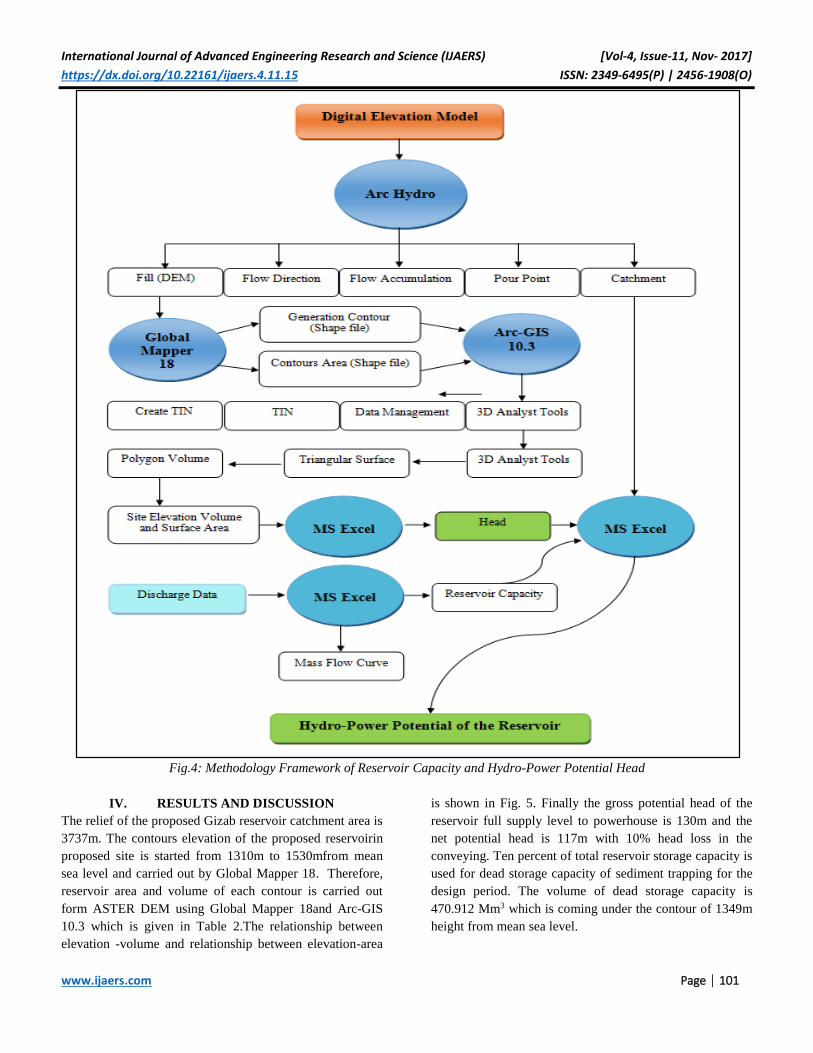
International Journal of Advanced Engineering Research and Science (IJAERS) [Vol-4, Issue-11, Nov- 2017]

https://dx.doi.org/10.22161/ijaers.4.11.15 ISSN: 2349-6495(P) | 2456-1908(O)

www.ijaers.com Page | 101

Fig.4: Methodology Framework of Reservoir Capacity and Hydro-Power Potential Head

IV. RESULTS AND DISCUSSION

The relief of the proposed Gizab reservoir catchment area is

3737m. The contours elevation of the proposed reservoirin

proposed site is started from 1310m to 1530mfrom mean

sea level and carried out by Global Mapper 18. Therefore,

reservoir area and volume of each contour is carried out

form ASTER DEM using Global Mapper 18and Arc-GIS

10.3 which is given in Table 2.The relationship between

elevation -volume and relationship between elevation-area

is shown in Fig. 5. Finally the gross potential head of the

reservoir full supply level to powerhouse is 130m and the

net potential head is 117m with 10% head loss in the

conveying. Ten percent of total reservoir storage capacity is

used for dead storage capacity of sediment trapping for the

design period. The volume of dead storage capacity is

470.912 Mm3 which is coming under the contour of 1349m

height from mean sea level.

International Journal of Advanced Engineering Research and Science (IJAERS) [Vol-4, Issue-11, Nov- 2017]

https://dx.doi.org/10.22161/ijaers.4.11.15 ISSN: 2349-6495(P) | 2456-1908(O)

www.ijaers.com Page | 102

Table.2: Contours Elevation, perimeter, volume and surface area of proposed Gizab reservoir

Contour Name Contour Elevation

(m)

Perimeter

(sq km)

Volume

( Mm3)

Surface Area (sq km)

1310 1310 0 0 0

1315 1315 13.67 3.633 0.866

1320 1320 42.914 20.354 4.608

1325 1325 32.796 67.914 10.849

1330 1330 37.824 129.316 13.043

1335 1335 41.243 200.831 15.099

1340 1340 45.301 284.119 17.477

1345 1345 50.918 379.391 20.308

1350 1350 52.088 490.504 22.861

1355 1355 68.907 640.255 27.266

1360 1360 82.246 790.932 30.948

1365 1365 92.505 956.390 34.211

1370 1370 103.76 1141.456 37.831

1375 1375 103.58 1335.163 40.461

1380 1380 108.42 1543.405 43.199

1385 1385 111.87 1758.255 45.502

1390 1390 129.6 2000.683 49.065

1395 1395 133.49 2248.741 51.769

1400 1400 137.12 2508.345 54.407

1405 1405 143.84 2781.632 57.305

1410 1410 153.51 3071.348 60.459

1415 1415 153.2 3372.173 63.308

1420 1420 159.39 3686.185 66.030

1425 1425 162.8 4013.118 68.960

1430 1430 166.98 4353.152 71.769

1435 1435 175.06 4709.118 74.822

Fig.5: Capacity-Elevation and Area-Elevation curve of proposed Gizab Reservoir

International Journal of Advanced Engineering Research and Science (IJAERS) [Vol-4, Issue-11, Nov- 2017]

https://dx.doi.org/10.22161/ijaers.4.11.15 ISSN: 2349-6495(P) | 2456-1908(O)

www.ijaers.com Page | 103

The mean monthly discharges are given in Table.3 the

maximum discharge is 310.347 m3/s in the month of June

and the minimum discharge is 30.119 m3/s in the month of

December. The average discharge of 12 month is 100.899

m3/s. The reservoir storage capacity form the mean

monthly inflow is driven from mass curve is 1114.356 Mm3

Fig.6. Also the reservoir storage capacity is driven

analytically from monthly mean inflow Table.3.

Table.3: Mean monthly inflow and propose Gizab reservoir capacity

Date Inflow in

m3/s

Inflow in

Mm3

Demand in

m3/s

Demand in Mm3 Deficit In

Mm3

Surplus in

Mm3

Jan. 32.465 86.955 100 262.660 175.705

Feb. 36.081 93.523 100 262.660 169.137

Mar. 38.577 103.326 100 262.660 159.334

Apr. 55.657 149.073 100 262.660 113.587

May. 55.227 133.606 100 262.660 129.054

Jun. 178.966 479.344 100 262.660 216.684

Jul. 310.347 804.419 100 262.660 541.759

Aug. 240.462 644.053 100 262.660 381.393

Sep. 105.050 272.290 100 262.660 9.630

Oct. 97.372 260.801 100 262.660 1.859

Nov. 30.119 80.670 100 262.660 181.990

Dec. 30.467 78.971 100 262.660 183.689

Total 1114.356 1149.465

Fig.6: Mass inflow curve diagram of Gizab reservoir

Based on the flow rate and estimated net available water

potential head 117 m the assessed hydropower potential is

calculated using Eq. (3) as 91.822 MW. Francis turbine has

selected for this study from turbine selection chart and the

hydraulic efficiency of the turbine is 80%. The analysis

shows that the Gizab reservoir has a good storage capacity

with a good water potential head for the generation of

hydropower establishment.

International Journal of Advanced Engineering Research and Science (IJAERS) [Vol-4, Issue-11, Nov- 2017]

https://dx.doi.org/10.22161/ijaers.4.11.15 ISSN: 2349-6495(P) | 2456-1908(O)

www.ijaers.com Page | 104

V. CONCLUSION

The reservoir capacity is the most important aspect for

hydrologic design.

The reservoir capacity is design for mean monthly

inflow data of several years using Mass Curve method

and the storage capacity is 1114.3 Mm3.

The gross storage volume of the proposed Gizab

reservoir is 4709.118 Mm3 and carried out from

ASTER DEM using Global Mapper 18 and Arc-GIS

10.3.

The gross potential head of the reservoir full supply

level to powerhouse is 130m and the net head for the

generation power is 117m with 10% head loss of gross

potential head at system operation.

The Francis turbine with 80% efficiency has used for

the study.

At available head with use of Francis turbine and its

efficiency of 80%, the hydropower potential is 91.822

MW.

REFERENCES

[1] Magome J, Ishidari H, Takeuchi K (2003). “Method of

Satellite Monitoring of Water Storage in Reservoirs

for Efficient Regional Water Management” Water

Res. Systems-Hydrological Risk, Manag.

[2] Salami Y, Nnadi F (2012). “Seasonal and Inter-annual

Validation of Satellite-Measured Reservoir Levels at

the Kainji Dam”. Int. J. Water Res. Environ. Eng.,

4(4): 105-113.

[3] Bharali Biswadeep (2015). “Estimation of Reservoir

Storage Capacity by using Residual Mass Curve”

Journal of Civil Engineering and Environmental

Technology., 2(10): 15-18.

[4] Sharma K.R., Sharma .K.T (2008). “Irrigation

Engineering Including Hydrology” S. Chand &

Company PVT.LTD, Rama Nagar, New Delhi-

110055.

[5] Garg. K.S ( 2016). “Irrigation Engineering and

Hydraulic Structures” Khanna Publishers Daryangani,

New Dehhli-110002.

[6] Pumnia.B.C, (2009).” irrigation and water power

engineering”; Laxmi publication (P) ltd; New Delhi,.

International Journal of Advanced Engineering Research and Science (IJAERS) [Vol-4, Issue-11, Nov- 2017]

https://dx.doi.org/10.22161/ijaers.4.11.16 ISSN: 2349-6495(P) | 2456-1908(O)

www.ijaers.com Page | 105

Pronunciation Remedy of Scientific Plants Names

with Pair Exercise Using Flash card Media at

Students Plant Taxonomy Course Pujiastuti, Imam mudakir, Iis Nur Asyiah, Siti Murdiyah, Ika Lia Novenda, Vendi Eko

Susilo

Lecturer in Biology Education, Faculty of Teacher Taraining and Education,University of Jember, Indonesia

Abstract— The botanical nomenclature is a part of plant

taxonomy.International communications of the name of

plants in the oral and written forms are arranged in the

botanical nomenclature system, using the scientific names

of plants in Latin or Latinized language. From the point of

view of Indonesian language the oral form or the

pronunciation of the scientific names of plants are not

always similar to Reviews their written form. The written

form and the oral forms of scientific names of plants are

arranged in the chapter of Pronunciation of the Scientific

Names of Plants. In fact it was found that the

pronunciations of the scientific names of plants are often

pronounced wrongly by about 57.2% of the students. The

improvement steps in terms of students' abilities in

pronouncing the scientific names of plants are needed to be

done using flash card media containing pictures and the

scientific names of plants. The research result shows that

after four training periods, the couple training using flash

cards media can decrease the range of errors in

pronouncing the scientific names of plants made by the

students. The number of the students who Pronounce the

scientific name of plants wrongly Decrease from the

number of 57.2% into the number of 9.7%. As many as 17

scientific names of plants that are pronounced wrongly by

the students now Decreased into 14 scientific names, from a

total of 30 names.

Keywords— pronunciation, the scientific names of plants,

flash card.

I. INTRODUCTION

The nomenclature of plants is a part of Plant Taxonomy.

The scientific names of the plants that are written in Latin

or Latinized language have a different character with the

Indonesian name or region. The scientific names in Latin,

often differ between the written form and the oral form (or

the pronunciation), so it can be something difficult for the

students. The fact shows that college students do mistakes

in pronouncing certain names of plants which have been

stipulated in the scientific nomenclature. For example, the

name Rhoeodiscolor,where the letter oe onword

Rhoeoshould be spoken e, but it is pronounced oe.by 85%

of the students, whileonly 15% of students who pronounce

it correctly. Likewise for the other names,error rate

ofpronunciation is also high. Education Workforce

Institutions like FKIP has the dutyto prepare educators to

be. Errors that occur in the pronunciation of scientific

names of plants among college students, must be

minimized, even should be eliminated. Errors that occur

among prospective teachers, can cause errors among the

students at the school, later in life.

Based on the description above, this paper discusses about

the efforts made and implemented in Biology Education

Study Program (P.BIO) FKIP University of Jember,

particularly in Plant Taxonomy Course, in terms of

pronunciationof the scientific names of the plants. This

work is done in order to minimize pronunciations errors of

scientific names of plants among students that are going to

be teachers.

Pronunciationof the scientific names of plants

Scientific names of Plantsare the names that are known by

the whole world. The scientific naming of plants are based

on the rules that have been defined in the International

Code of Botanical Nomenclature (ICBN). The scientific

names of plants use Latin words or Latinized words from

some other languages (Tjitrosoepomo, 2009). New

information about the type of plant, or a scientific name

change must be authorized by ICBN (Llamas, 2003). One of

the methods of Latin pronunciation method agreementused

todayis the English method. The use of English method of

pronunciation has the consequence of following the English

words pronunciation. Some general rules for the

pronunciation of the scientific names of plantsare;

International Journal of Advanced Engineering Research and Science (IJAERS) [Vol-4, Issue-11, Nov- 2017]

https://dx.doi.org/10.22161/ijaers.4.11.16 ISSN: 2349-6495(P) | 2456-1908(O)

www.ijaers.com Page | 106

1. If a single consonant exists between two vowels,

consonant is read with vowels that follow it. Example:

acer, is read a-cer

2. If two consonants exist between two vowels, then the

first consonant is read with the first vowel, and the

secondconsonant is read with the second vowel.

Example: albidus, is read albidus.

3. The final vowel, is pronouncedin a long way. Example:

Alsine,is read al-si-nee,except the letter a,is sounded

with ah.

4. Letter ae and oe are pronounced with a longe.

Example:laevis is read lee-vis; rhoeas, is read ree-as.

5. The letter C is read with the sound s,letter gis read with

the sound j if they meet the letterse, i, y, ae or

oe.Example: Cedrus, see-drus; cyaneus, si-ne-us;-a

g,eneralisje-ne-ra-lis. But the letter C will be read with

the sound of k,if it is followed by the letters a, o,or

u.Example: Candidus, is readkan-in-dus

6. If a word begins with one of these consonant pairs, the

first letter is not pronounced: cn, ct, gn, mn, pn, ps, pt,

tm.Example: cnicus, is read nicus; ctenium is read te-

ni-um; psyllium,is readsil Li-um.

7. If a couple of letters ti,followed by the vowels: a, u, e,

o. then t is sounded s example: Opuntiais read Opunsia

(Radford, 1986) as well as some other rules, which

generally are used to be spoken correctly.

Exercise In Couples

Pair pronunciation exercise of the scientific names of

plantsis intended to stimulate pairs mutual peer correction.

In essence, this activity gives students opportunities to

practice activities pronouncing the scientific names of

plants, more often. Mispronounce done by students, are

expected to be corrected by the partner of training.

Practicing in pairs with friends, give a better chance of

success, rather than if it is performed alone. Learning in this

manner substantially is similar to the discussion. Discussion

train students to get used to listen to the others’ opinions,

even though it may be different from their own opinions; it

also trains students to tolerate (Asmani 2010). Cooperation

learning oriented between friends is essentially the

Cooperative Learningmodel. Cooperative learning model,

not only helps the students understand difficult concepts,

but also improves the cooperative ability, social skills, and

thinking ability (Susilo, 2007). Such conditioning effort is

one of the classroom management elements. Classroom

Management conducted by educators, aims at creating a

good social atmosphere in the classroom, so that it can

provide the satisfying conditions, discipline atmosphere,

intellectual, emotional, positive attitude and appreciation for

the learners (rusydie, 2011). Intellectual, emotional, positive

attitude and appreciation of the learners, enabling the better

achievement of learning goals. Errors that are occurred, are

expected to be minimized, in this case primarily scientific

errors in pronouncing the names of the plants .

Media flashcard

Mediacomes from the Latin wordmediuswhich mean is

central, introduction or intermediary. Learning media is a

means of intermediaries in the learning process. Benefits of

the media, are: it can clarify the message, overcome the

limitations of space, time and senses, it also gives rise to

common perception, stimulates learning, creates a positive

attitude toward the subject matter and provides the

conditionof direct interaction between learners and learning

resources (Daryanto, 2011). Flashcardmedia is a small card

containing images, texts, or symbolsthat reminding or

guiding students to something related to the pictures. The

card size is usually 8 x 12 cm, or can be adjusted to the size

of the class face (Arsyad, 2009). The images that are used in

the cards can be selected in the form of photographs. A

representative photograph gives an overview that can

represent the real thing, gives the same perception to the

learner. Photos that are selected and used in accordance

with the specified learning objectives, can fulfill their

functions to raise the motivation and interest of the students

(Arsyad, 2009). Motivation determines the learning

persistence, someone who has been motivated to learn

something, will give his effort to obtain good results (Uno,

2011). Photos of a wide variety of plants are equipped with

regional and scientific names. Some of the plants that are

shown in the photos can be found in the students

surrounding environments, and some of them are still

unfamiliar for the students or they just seen them for the

first time.Photos of the new plants that are first seen by the

students, attract the students’ attention, they give a real

picture of what is imagined by the students from the names

that they have ever heard or read. Watching photos of plants

helps the students to remember the characteristics or the

names of plants better than hearing or reading.Dale put the

visual symbols experience more concrete than verbal

symbols (Daryanto, 2011). Photographs of plants which

accompanied the plant names both local and scientific

names, givemore impressionfor students. This impression is

an extrinsic factors that can encourage students to learn

more hard and dilligent (Uno, 2011).

Plant Taxonomy Courses

Plant Taxonomy Course is one of the subjects in the

Biology Education Studies Program at FKIP University of

Jember. This course has 4 SKS (Semester Credit Units) ,

with details of 2 credits of practicum (1 time meeting), 2

International Journal of Advanced Engineering Research and Science (IJAERS) [Vol-4, Issue-11, Nov- 2017]

https://dx.doi.org/10.22161/ijaers.4.11.16 ISSN: 2349-6495(P) | 2456-1908(O)

www.ijaers.com Page | 107

credits lecture consists of two meetings a week. Total

meetings are 3 times in a week. Plant Taxonomy Class

syllabus contains competencies that must be achieved by

the student after taking this course, those competencies are

as follows: After taking this course, students can analyze

the diversity of plants based on the classification system of

plants and can apply it in daily life. Furthermore, to achieve

these outcomes, the student must have the ability to

describe, identify, apply the nomenclature of plants,

including mention the scientific names of plants properly.

Plant taxonomy is the main part of the Plant Systematic

consists of four components: Descripsion, Identification,

Nomenclature, Classification (Simpson, 2006). Formal

naming plants and all the rules have been set in the ICBN.

The scientific name of the plant is set on the term ofwriting

and pronunciation.

The fact that encountered in the implementation of Plant

Taxonomy courses, mainly on the part of the nomenclature,

students often make a serious mistake when theypronounce

the scientific names. The main cause is due to a lack of

knowledge, lack of exercise on students, because between

words and sounds are not always similar according to the

Indonesian character. Mistakes made by students even have

been donethey were at the previous education level. Errors

that have been occurred for a long time then become a habit

for the students and it is very difficult to be repaired. That is

why it needs special trick to fix it. The way in pronouncing

the scientific names, as well as the language, needed to be

practiced repeatedly. Exercises are performed with friends

in pairs, where each other give correction and motivation.

Practice with friends is more comfortable for the students

because it reduces inhibitions and embarrassment when they

are making mistakes, rather than if it is corrected by the

teacher. How learning takes place, will determine the

learning quality of the learners. Beside affected by external

factors learning quality of the learners isalso affected by

individual factors of the learners, such as difficult to

concentrate, less passionate, selfish, shy or less socialize

with friends (Rusydie, 2011). Practicing in pairs, is

expected to minimize those factors. Creating a pleasant

situation in the learning process, is an attempt to attract

learners attention to what they learn. Utilization

offlashcardmedia that contains the scientific name of plants

that are concerned with image (an image from the photo),

beside increase the students’ interest, also help the students

to remember the names and characters of the plants. The

learning activity is a complex process that involves several

aspects and components that mutually affect each other, so

it requires good management skill (Sobri et al, 2009).

Integrating pair exercise and the use offlashcardmedia is an

effort in managing instructional activity to achieve

thelearning objectives.

II. METHODOLOGY

Application of cooperative learning with pair exercises

using flash card media containing photographs and

scientific names and characters of plants in the subject of

Plant Taxonomy, aims at repairingthe pronunciation errors

of the scientific name of plants that are often done by the

students. Furthermore, to achieve competence in Plant

Taxonomy courses generally. Cooperative learning with

pair exercises usingflashcardmedia,in the subject of Plant

Taxonomy consider the aspects that are contained in the

National Education Act No. 20 of 2003 (Iskandar, 2011).

Those aspects are included in the lesson plans of learning

and applied in the learning process and evaluated at the time

or at the end of the lesson. Stepstaken in this study were as

follows:

As many as 40 students of Plant Taxonomy course are

required to read the scientific names of plants at the

beginning of the course, as the initial data. They do this by

saying / reading 30 scientific names of plants in rotation and

marked on a list of names that are spoken wrongly by the

students. After all students read and marked on the names

that are spoken wrongly by the students, then counted how

many students who do the mistakes in reading the scientific

names of plants. Errors that are already on the list, then

discussed based on the theory of plant nomenclature set out

in the ICBN. After the rules of nomenclature and

pronunciation / pronunciation havebeen known and

mastered by the students, then the students are trained to

pronounce the name.

Flash cardplantsnames are made by the students. Each

student make a card with the prefix letters in the order, each

letter on 5 different plants names, so the number of flash

cardsthat are made are as many as 5 x 26 = 130 pieces for

one series. As many as 200 pieces cards are made by 40

students by repeating the series, each student makes 5

pieces with different name for every letter. Plants cards that

have been made by students, then verified and compliance

with the provisions, including the names which are often

pronounced wrongly.

The implementation is set as follows: 40 students divided

into five major groups, each group consists of 8 students.

Each group set themselves sitting opposite in pairs. A pair

of students hold 10 sheets of flash card/ card. One person

practice reading scientific name, while his partner to listen

and observe. if something goes wrong, the partner tries to

correct. This be repeated in 5 minutes duration, then change

the turn with their partner. After completion of the partner

turn, exchange the cards with another couple in the same

International Journal of Advanced Engineering Research and Science (IJAERS) [Vol-4, Issue-11, Nov- 2017]

https://dx.doi.org/10.22161/ijaers.4.11.16 ISSN: 2349-6495(P) | 2456-1908(O)

www.ijaers.com Page | 108

group, and it is repeated in the same way for each pair.

Once completed in one group, exchangethe cards with

another group, until all groups have read all the cards

available. The exercise is repeated until 4 meetings.

Evaluation was conducted in the same manner by obtaining

initial data. The results then compared with the initial data,

the analysis is done for each of the representatives of the

plants names, to count how many students pronounce

wrongly. After it is viewed as a whole, see how many

pronunciation errors made by the students after being

trained in learning. Interviews are done to the students, at

the end of the study. Interviews provide an opportunity for

students to express what they feel after what happened in

the learning with in pairs training methods using flascard

media.For students who do not have the opportunity to

speak, are excused to write their opinion to be submitted to

the lecturer.

III. RESULTS AND DISCUSSION

After the evaluation to the pronunciation of scientific names

of plants, it was obtained 17 scientific names of plants that

were pronounced incorrectly by some students of 30

scientific names of plants selected. The result can be seen in

the following table;

Table.1: Scientific names of plants spelled wrongly and the number of student who pronounce wrongly

No. The scientific name of plants beginning

the end of the

course

1 Caesalpinia pulcherima 32 4

2 Eugeniaaromatica 28 2

3 Flacourtia rukam 34 8

4 Gnetum gnemon 26 4

5 Hedychium coronarium 12 8

6 Ipomoea aquatica 37 4

7 Justica brook 21 7

8 Kaempferia rotunda 19 5

9 Leucaena glauca 21 4

10 Morinda citrifolia 8 0

11 Nephelium litchi 7 4

12 Opunthe vulgaris 32 4

13 Psidium guajava 29 0

14 Pteris ensiofrmis 29 0

15 Psilotum nudum 29 2

16 Rhoeo discolor 34 7

17 Triticum aestivum 12 4

Total 389 66

average 22 88 3.88

Data on tabel.1 showed that at the beginning of the lecture,

of 30 scientific names of plants chosen, there are 17 names

of plants were pronounced incorrectly by the general

students, while the rest, which were 13 plants names (not

diagramed), generally pronounced correctly by students, or

pronounced incorrectly by no more than 3 students. The

error occured on the pronunciation of the underlined letter

in tabel.1 above. At the beginning of the term, from 30

scientific names of plants that should be read by all the 40

students, there were 17 scientific name spelled wrongly by

more than 3 students. Data show that 17 scientific names

plants pronounced incorrectly by an average of 22.88

students, which means 57.2% of the 40 students.

After the students getting an explanation about the

correct pronunciation, and after practicing in pairs

usingflashcardmedia during the four periods, the error were

greatly reduced. From 17 scientific names of plants that

were spelled wrongly by an average of 22.88 students,

which means 57.2% of the 40 students, after the learning

process the number decreased into 3.88 students, which

means that 9.7% of 40 students. From the information

obtained from the students, it was known that they

pronounce the namely wrongly way since before entering

International Journal of Advanced Engineering Research and Science (IJAERS) [Vol-4, Issue-11, Nov- 2017]

https://dx.doi.org/10.22161/ijaers.4.11.16 ISSN: 2349-6495(P) | 2456-1908(O)

www.ijaers.com Page | 109

the college level. Although they pronounce the name

correctly, they claimed that they did not to know

grammatical rules. Their mistakes sometimes were

corrected by a friend or an assistant on the course before the

taxonomy of the plants, then they changed the

pronunciation. But then they forgot again afterwards. After

learning grammar pronunciation rules, the student tried to

change the wrong habits with practicing in pairs with

friends. Practicing in pairs is a more effective way rather

than discussing with the crowd. The discussion becomes

ineffective if the group is too large, the group could be

dominated by certain people who like to talk (Asmani,

2010). Practicing in pairs is also approved by the students, it

gives them the opportunity to develop their potential.

Atmosphere of learning and the learning process that allow

students to actively develop their potential, is one of the

things implied in the Act Sis Dik Nas 20 yrs, 2003

(Iskandar, 2011). Learning is doing and it is a process that

makes the learners more active, means that learners should

dominate the activity (Sardiman, 2007).

Flashcard media give a more concrete pictures of the plants

studied, and also help the students to remember how to

pronounce the names correctly. In general, the students

stated that the Flash card containing photos of plants are

very helpful to remind how to pronounce the scientific

name, especially if they can see the plantseveryday in their

surrounding environments. Data showed that as many as 3

of 17 plants, even pronounced correctly by all of the

students. Those plant areMorindacitrifolia, Psidium

guajava and Pterisensiformis.the first 2 plantsmentionedare

well-known by all students, because there are many of them

that can be found in the daily life.The picture of Dale cone

experience put the visual symbol more concrete than verbal

experience (Daryanto, 2011). Visual symbols contribute

larger memory than the verbal symbol. Pictures from the

photo illustrate the plant are easily remembered by the

students, and it also make them easier in considering how to

pronounce it. Visualizing images in the mind is also called

visualimagery, it is one way to improve memory (Waid,

2011). Practicing pronounce the scientific names correctly

and repeatedly, is the way of habituation. The more frequent

the practice, the more accustomed students to pronounce

correctly. It is proved that after practicing repeatedly,

during the four periods, errors which were performed by as

many as 22.88 or 23 students in the beginning, were

reduced to an average of 3.88 or 4 people. Information

obtained from the students both orally and in written,

providing information that practicing with friends provides

emotional flexibility, eliminates awkward feeling and

provides free-error-correcting by friends. Media containing

photos of plants studied were also very helpful in

remembering the object and pronouncing the scientific

names correctly. Considering the object of the photograph is

the mental activity of each individual learner. Practice

saying in pairs is a group activity. In Teaching and Learning

Activities (KBM), the approach taken by the lecturer will

produce various learners activities, whether individually or

in groups, and the combination of both will produce better

learning outcomes (Djamarah, 2002). It was proven that

after the end of the lesson students pronounce the scientific

names of plants wrongly, which had an average of 22.88

students from 40 students or 57.2% down to an average stay

of 3.88 students from 40 students, or 9.7%. Plant Scientific

namesthat were spelled wronglywere also decreased from

17 names into 14 names.

IV. CONCLUSIONS

1. Learning Application with pair exercise

usingflashcardmediacan fix the faulty pronunciation of

scientific names of plants on students who took Plant

Taxonomy course. Error which was previously

performed by an average of 22.88 from 40 students or

57.2% of students, decreased to an average of 3.88 out

of 40 students, or 9.7%.

2. The number of the scientific names of plants which were

spelled wrongly by most of the students, decreased from

the number of 17 names into 14 names. Those 14

scientific names of plants were still pronounced

incorrectly by a few students.

REFERENCES

[1] Arsyad, A. 2009. MediaLearning,119-120. Jakarta:

King Grafindo Persada.

[2] Asmani, JM 2011. Tips to Master Inspiring, Creative

andInnovative,138-142. Jogjakarta: Diva Press.

[3] Daryanto.2011. LearningMedia,11-13. Bandung: PT

Sarana Tutorial Conscience prosperous.

[4] Djamarah, SB, Zain, A. 2002. Teaching and

LearningStrategies,129-130. Jakarta: Rineka

Reserved.

[5] Llamas, KA 2003. Tropical Flowering Plants: a guide

to identification andcultivation,19-20. Cambridge:

Timber Press, Inc.

[6] Muhaimin, Akhmad, A. 2011. EducationFrees,15-18.

Jogjakarta: Ar-Ruzz Media.

[7] Radford, AE 1986. Fundamentals of

PlantSystematics,98-103. New York: Harper & Row

Publishers Inc.

International Journal of Advanced Engineering Research and Science (IJAERS) [Vol-4, Issue-11, Nov- 2017]

https://dx.doi.org/10.22161/ijaers.4.11.16 ISSN: 2349-6495(P) | 2456-1908(O)

www.ijaers.com Page | 110

[8] Rusydie, S. 2011. Principles of

ClassroomManagement,77-100. Jogjakarta: Diva

Press.

[9] Sardiman, AM 2007. Interaction and Motivation

andLearning,97-98. Jakarta: King Grafindo Persada.

[10] Simpson, Michael G. 2006. PlantSystematic,9-10.

Canada: Elsevier Academic Press.

[11] Sobri, Jihad, A., Rochman, CH 2009.

EducationManagement,23-34.Jogjakarta: Multi

Pressindo.

[12] Susilo, H.2007. Thinking Ability Development

danAssesmen preformance Cooperative Strategy

Papers submitted in Authentic Assessment Training

and Capability Development of Thinking and

Implementation in Cooperative Learning. 2007 at the

University of Muhammadiyah Malang, Malang,

January 29.

[13] Tjitrosoepomo, G. 2009. General Taxonomy:

Fundamentals of PlantTaxonomy,81-82. Yogyakarta:

Gadjah Mada University Press.

[14] Uno, HB 2011.Motivation Theory

andMeasurement,23-32. Jakarta: PT Earth Literacy

[15] Waid, A. 2011. Reveals the Secrets of

LearningJews,165-166. Jogjakarta: DIVA Press.

International Journal of Advanced Engineering Research and Science (IJAERS) [Vol-4, Issue-11, Nov- 2017]

https://dx.doi.org/10.22161/ijaers.4.11.17 ISSN: 2349-6495(P) | 2456-1908(O)

www.ijaers.com Page | 111

The Effect Analysis of Traffic Volume, Velocity

and Density in Dr.Siwabessy Salobar Road Selviana Walsen, La Mohamat Saleh

Civil Engineering of Politeknik Negeri Ambon

Abstract—Traffic density has been considered to be

affected by the traffic volume and the traffic velocity. This

study focuses on investigating the roles of both aspects on

the traffic density along the street of Dr. Siwabessy, from

Ambon City to Air Salobar or vice versa. This street has

been considered to be one busy street in Ambon City with

various vehicles passing by along with the crowded

pedestrian activities and with new business centrals (e.g.

school) along the road describing the complexity of the

street traffics. From the study, it was found that the traffic

velocity was statisitically the more significant factor in

determining the traffic density compared to the traffic

volume following the use of the coefficient regression

model. The other finding is that the traffic along the street

can be classified to be under-saturated

Keywords— Traffic volume, traffic velocity,

traffic density, regression model.

I. INTRODUCTION

According to Mashuri (2012) more and more community

activity affect the characteristics of traffic flow like speed,

volume and traffic density. According to Ekawati et al

(2014), one of the main causes of traffic jam is

unbalanced road capacity with an increasing number of

vehicles. Dr. Siwabessy street in Air Salobar is one of the

important streets in Ambon City, which serves the traffic

flow from Ambon to Air Salobar. This road is used as a

connecting lane from Ambon to Nusaniwe Sub-district. In

recent years population growth in Nusaniwe sub-district

has been caused the significant increase of vehicles

through Dr. Siwabessy street. On the other hand, traffic

jam caused by the activity from several new office and

school building at this area. So Dr. Siwabessy highway

segment will be more crowded because of the volume of

vehicles and will affect to the capacity of existing

highway. By looking at these conditions it is necessary to

do a study to determine the speed, volume and density of

roads Dr. Siwabessy-Air Salobar which is a highway that

always passes many types of vehicles, as well as daily

activities of society. So we will know the road capacity

feasibility.

II. LITERATURE

2.1 Highway Definition

Highway are transport infrastructures covering all parts of

the road, including auxiliary buildings and equipment

intended for traffic. The other hand it means a place

passed by vehicle that through a road so that the highway

is a very important in all aspects of life. The highway is

also affect of an economy and the progress of a country.

2.2. Capasity

The capacity of the highway is the maximum number of

vehicles that can pass through the road within a period of

one hour without causing traffic jam (Warpani, 1985).

According to MKJI (1997) capacity is the maximum

current vehicle through a path that can be maintained per

unit of hours under certain conditions. The basic equation

for calculating road capacity in Indonesian Road Capacity

Manual (1997) is:

C : Co x FCw x FCSP x FCSF x FCCS

with :

C : road capacity (smp/hour)

Co : basic capacity (smp/hour)

FCw : preparation of wide traffic lane factor (smp / hour)

FCSP: direction separation adjustment factor

FCSF :adjustment factor due to abstacles

FCCS :adjustment factor of city capacity

For urban road capacity, basic capacity can be seen in

table 2.1

Table.2.1 The Basic Capacity of Urban Roads

Type Basic capacity (smp/hour)

four-divided lane 1650/ lane

Four-undivided lane 1500/lane

Two undivided lane 2900/two lane

International Journal of Advanced Engineering Research and Science (IJAERS) [Vol-4, Issue-11, Nov- 2017]

https://dx.doi.org/10.22161/ijaers.4.11.17 ISSN: 2349-6495(P) | 2456-1908(O)

www.ijaers.com Page | 112

Table.2.2: Preparation of Wide Traffic Lane Factor (fcw)

Type effective traffic width,

(Wc) (m)

FCw

four-divided lane 3.00

3.25

3.50

3.75

4.00

0.92

0.96

1.00

1.04

1.08

Four-undivided lane 3.00

3.25

3.50

3.75

4.00

0.91

0.95

1.00

1.05

1.09

Two undivided lane 5

6

7

8

9

10

11

0.56

0.87

1.00

1.14

1.25

1.29

1.34

Table.2.3: Direction Separation Adjustment Factor (FCsp)

direction separation (SP)

% - %

50-50 55-45 60-40 65-35 70-30

FCsp

(2/2) 1.00 0.97 0.94 0.91 0.88

(4/2) 1.00 0.985 0.97 0.955 0.94

Table.2.4: Adjustment Factor Due to Abstacles

Type Side barriers

Class

FCSF

Effective width (Ws) (m)

≤ 0.5 m 1.0 m 1.5 m ≥ 2 m

4/2 D VL

L

M

H

VH

0.96

0.94

0.92

0.88

0.84

0.98

0.97

0.95

0.92

0.88

1.01

1.00

0.98

0.95

0.92

1.03

1.02

1.00

0.98

0.96

4/2UD VL

L

M

H

VH

0.96

0.94

0.92

0.87

0.80

0.99

0.97

0.95

0.91

0.86

1.01

1.00

0.98

0.94

0.90

1.03

1.02

1.00

0.98

0.95

(2/2 UD) atau

jalan satu

arah

VL

L

M

H

VH

0.94

0.92

0.89

0.82

0.73

0.96

0.94

0.93

0.86

0.79

0.99

0.97

0.95

0.90

0.85

1.01

1.00

0.98

0.95

0.91

Table.2.5: Adjustment Factor of City Capacity (FCcs)

City size FCcs

< 0.1 0.86

0.1-0.5

0.5-1.0

1.0-3.0

0.90

0.94

1.00

International Journal of Advanced Engineering Research and Science (IJAERS) [Vol-4, Issue-11, Nov- 2017]

https://dx.doi.org/10.22161/ijaers.4.11.17 ISSN: 2349-6495(P) | 2456-1908(O)

www.ijaers.com Page | 113

> 3.0 1.04

2.3. Traffic Volume

The parameter used to determine daily traffic patterns is

an average traffic (LHR), LHR obtained by traffic

monitoring for 24 hours, in a few days and the result is

averaged, expressed in vehicle / day or day / day can be

calculated by the formula:

T

NQ

with :

Q : volume

N : number of vehicle

T : observation time

2.4. Velocity

Speed is the ratio between distance and time. The formula

for calculating speed that is:

T

SV ;

with:

V : velocity (km/hour)

S : distance (km)

T : time(hour)

2.5. Density

Traffic density is the number of vehicles that exceed the

capacity of the highway. Density can be calculated based

on speed and volume.

Table.2.6: Q/C Ratio

Q/C Condition

< 0,8 road segment can still serve the

volume requirements of vehicles

passing through the road

0,8 -

1,0

unstabled condition ,ecause the

condition of the road segment can not

accommodate the number of vehicles

passing through the road

> 1,0 a condition in which the road segment

can accommodate the movement of

vehicle volume.

The relationship between volume, speed, and density is as

follows:

Us

QD

with :

D : Traffic density (vehicle/hour)

Q : Traffic volume (vehicle/km)

Us : mean traffic velocity of space (km/hour)

2.6. Saturation ratio

Saturation ratio defined as the ratio of traffic

flow Q (smp / hour) to capacity C (smp / hour) is used as

the main factor in determining the level of road segment

performance.aturation is defined as the following

formula;

DS = Q/C

with :

Q : traffic flow

C : capacity

2.7. Relation between Volume, Speed, and Traffic

Density

The mathematical relationship between speed, volume,

and density can be expressed by the following equation:

DxSQ

with:

Q : volume (SMP/hour)

D : density(vehicle/km)

S : speed (km/hour)

2.8. Passenger Car Unit

The passenger car unit abbreviated as SMP (indonesian

factor) is the unit of vehicle in the traffic flow which is

equivalent to the light vehicle / passenger car, using the

passenger car's equivalence or multiplier factor of the

vehicle type into one unit of SMP, where the SMP is

influenced by the type / type vehicles, vehicle

dimensions, and motion capabilities. The quantities of

passenger car units vary according to the Indonesia Road

Capacity Manual 1997 shown as follows:

Table.2.2: SMP Factor

Vehicle (smp)

HV 1,20

LV 1,00

MC 0,25

Table.2.3: Classification of Vehicles

Classification of

vehicles

Vehicle

HV Trucks and Buses

LV Passenger Car, Mini

Bus, Truck pick up

MC Motorcycle

International Journal of Advanced Engineering Research and Science (IJAERS) [Vol-4, Issue-11, Nov- 2017]

https://dx.doi.org/10.22161/ijaers.4.11.17 ISSN: 2349-6495(P) | 2456-1908(O)

www.ijaers.com Page | 114

III. METHOD

3.1 Location

This research is located on Jln Dr Siwabessy - Air

salobar of Ambon Street

3.2 Research Time

This research was conducted on 30 August 2017 until

September 2017

3.3 Data Type

1. types of data used are as follows:

a. Traffic Volume

b. Speed

c. Road geometric

3.4. Data Analysis Techniques

a. Data Processing Technique

This writing uses the data obtained, with the aim of

obtaining an effective approach based on the existing

theoretical studies with the following survey steps:

Preliminary studies

-Preliminary study is the process of collecting data to

support this writing

- Library Studies

Conducted by collecting references related to the

support of writing, which is a theoretical study.

- Data Compilation

Data compilation, is basically a process of collecting,

processing and reporting data to get the final result of

data half-baked ready to be processed at the stage of

data analysis.

- Data Processing and Analysis.

Data processing is an activity for converting raw data

that has been obtained into a standard format

approached by theoretical studies.

IV. RESULTS AND DISCUSSION

4.1. Traffic Volume Analysis

The number of motor vehicles operating on Dr.Siwabessy

road is obtained based on survey during peak hours, in the

morning, afternoon and evening, are presented in Table

4.1.

Based on survey results of traffic volume on road Dr.

Siwabessy can be seen that the maximum vehicle volume

is at 08.00-09.00 with the direction of Ambon - Air

Salobar of 1909 vehicles / hour and at 07.00-08.00 with

the direction of Air Salobar - Ambon of 1283 vehicles /

hour. Subsequently converted into units of passenger cars

(smp) using the Highway Manual Capacity Indonesia

1997 for each road segment.

Based on the table 4.5. can be seen for Dr.Siwabessy

road segment ratio has less than 1, this indicates that the

condition of traffic flow is still below saturated From the

above table it is known that in the direction of Ambon to

Air Salobar vehicle speed is slower than the direction of

Air Salobar to Ambon, this is because vehicles entering

Air Salobar area are more dense than vehicles from

Ambon to Air Salobar.

Table.4.1: Traffic Volume of Dr.Siwabessy Road

Time

Traffic Volume (Vehicle/hour)

Ambon - Air

Salobar

Air Salobar -

Ambon

06:00 - 07:00 1062 622

07:00 - 08:00 1659 1283

08:00 - 09:00 1909 1003

09:00 - 10:00 839 506

10:00 - 11:00 923 819

11:00 - 12:00 1293 1222

12:00 - 13:00 1625 1001

13:00 - 14:00 1383 1160

14:00 - 15:00 1081 1129

15:00 - 16:00 481 1042

16:00 - 17:00 1085 999

17:00 - 18:00 1148 1102

18:00 - 19:00 1021 1262

International Journal of Advanced Engineering Research and Science (IJAERS) [Vol-4, Issue-11, Nov- 2017]

https://dx.doi.org/10.22161/ijaers.4.11.17 ISSN: 2349-6495(P) | 2456-1908(O)

www.ijaers.com Page | 115

Table.4.2: Dr.Siwabessy Road Traffic direction Ambon to Air Salobar (smp / jam)

Time

Vehicle Classification

Total HV LV MC

06:00 - 07:00 10 594.1 238 842.1

07:00 - 08:00 12 1173.9 297.6 1483.5

08:00 - 09:00 13 957 375.6 1345.6

09:00 - 10:00 5 456.3 193.2 654.5

10:00 - 11:00 12 562.9 191.2 766.1

11:00 - 12:00 20 830.7 253.6 1104.3

12:00 - 13:00 22 1136.2 291.6 1449.8

13:00 - 14:00 14 890.5 273.6 1178.1

14:00 - 15:00 15 586.3 246 847.3

15:00 - 16:00 18 601.9 246 865.9

16:00 - 17:00 19 586.3 246 851.3

17:00 - 18:00 14 690.3 241.2 945.5

18:00 - 19:00 13 625.3 210.8 849.1

Table.4.3: Dr.Siwabessy Road Traffic Direction Air Salobar to Ambon (smp / jam)

Time

Vehicle Classification

Total HV LV MC

06:00 - 07:00 12 404.3 119.6 535.9

07:00 - 08:00 20 703.3 288.8 1012.1

08:00 - 09:00 8 616.2 208.4 832.6

09:00 - 10:00 5 308.1 105.6 418.7

10:00 - 11:00 8 591.5 142.4 741.9

11:00 - 12:00 12 742.3 255.6 1009.9

12:00 - 13:00 13 551.2 225.6 789.8

13:00 - 14:00 16 718.9 236.4 971.3

14:00 - 15:00 18 694.2 230.8 943

15:00 - 16:00 20 648.7 209.2 877.9

16:00 - 17:00 21 582.4 212 815.4

17:00 - 18:00 13 634.4 240.4 887.8

18:00 - 19:00 16 802.1 251.6 1069.7

4.2. Capasity Calculation

Table.4.4: Result of Road Capacity Calculation

Location

Basic

Capasity

Adjustment Factor

Road Capacity

(smp / hour)

(smp/hour)

Line

width

Separation of

direction

Side

Barri

ers

City

ratio

Dr. Siwabessy

Street

Ambon to Air

Salobar 2900 0.96 1 0.94 0.93 2433.77

Arah Air Salobar

to Ambon 2900 0.96 1 0.94 0.93 2433.77

International Journal of Advanced Engineering Research and Science (IJAERS) [Vol-4, Issue-11, Nov- 2017]

https://dx.doi.org/10.22161/ijaers.4.11.17 ISSN: 2349-6495(P) | 2456-1908(O)

www.ijaers.com Page | 116

Table.4.5: V / C Ratio Each Lane

Location Period Volume Capasity VCR Max

VCR

Dr. Siwabessy

Street

Ambon to

Belakang

Soya

Morning 691 3200.79 0.22

0.34 Noon 963.5 3200.79 0.30

Afternoon 1073.8 3200.79 0.34

Evening 776.5 3200.79 0.24

Belakang

Soya to

Ambon

Morning 1238.9 3200.79 0.39

0.45 Noon 1165.4 3200.79 0.36

Afternoon 1432.1 3200.79 0.45

Evening 1297 3200.79 0.41

4.3. Velocity analysis

Table.4.6: Velocity analysis at Dr.Siwabessy Street (Ambon-Air Salobar)

Period Time Mean

Speed

Space

Mean

Speed

Morning 42 42

Noon 42 42

Afternoon 48 48

Evening 44 44

Table.4.7: Velocity Analysis at Dr.Siwabessy Street (Air Salobar –Ambon)

Period Time Mean

Speed

Space Mean

Speed

Morning 47 47

Noon 49 49

Afternoon 49 49

Evening 46 46

Table.4.8: Traffic Velocity Recapitulation

Period

Velocity (Km/Hour)

Time Ambon - Air

Salobar Time

Air Salobar -

Ambon

Morning 0.00123 41.98 0.00109 47.11

Noon 0.00116 42.24 0.00117 48.89

Afternoon 0.00139 48.00 0.00120 48.89

Evening 0.00146 44.38 0.00117 46.17

Average 0.00131 44.15 0.00 47.76

4.4. Density Analysis

4.4.1. Calculating Traffic Density

Table.4.9: Calculation of Traffic Density of Road Sections Dr.Siwabessy Directions Ambon to Air Salobar.

Time Ambon - Air Salobar

Volume Velocity Density

06:00 - 07:00 842.1 41.98 20.06

07:00 - 08:00 1483.5 41.98 35.34

08:00 - 09:00 1345.6 41.98 32.05

09:00 - 10:00 654.5 41.98 15.59

International Journal of Advanced Engineering Research and Science (IJAERS) [Vol-4, Issue-11, Nov- 2017]

https://dx.doi.org/10.22161/ijaers.4.11.17 ISSN: 2349-6495(P) | 2456-1908(O)

www.ijaers.com Page | 117

10:00 - 11:00 766.1 41.98 18.25

11:00 - 12:00 1104.3 41.98 26.31

12:00 - 13:00 1449.8 42.24 34.32

13:00 - 14:00 1178.1 42.24 27.89

14:00 - 15:00 847.3 48 17.65

15:00 - 16:00 865.9 48 18.04

16:00 - 17:00 851.3 48 17.74

17:00 - 18:00 945.5 48 19.70

18:00 - 19:00 849.1 44.38 19.13

Table.4.10: Calculation of Traffic Density of Road directions Air Salobar to Ambon

Time Air Salobar - Ambon

Volume Velocity Density

06:00 - 07:00 535.9 47.11 11.38

07:00 - 08:00 1012.1 47.11 21.48

08:00 - 09:00 832.6 47.11 17.67

09:00 - 10:00 418.7 47.11 8.89

10:00 - 11:00 741.9 47.11 15.75

11:00 - 12:00 1009.9 47.11 21.44

12:00 - 13:00 789.8 48.89 16.15

13:00 - 14:00 971.3 48.89 19.87

14:00 - 15:00 943 48.89 19.29

15:00 - 16:00 877.9 48.89 17.96

16:00 - 17:00 815.4 48.89 16.68

17:00 - 18:00 887.8 48.89 18.16

18:00 - 19:00 1069.7 46.17 23.17

Fig.4.1: The Relationship between Predictions of Vehicle Density Using Regression Formula with the Calculation of Vehicle

Density

International Journal of Advanced Engineering Research and Science (IJAERS) [Vol-4, Issue-11, Nov- 2017]

https://dx.doi.org/10.22161/ijaers.4.11.17 ISSN: 2349-6495(P) | 2456-1908(O)

www.ijaers.com Page | 118

Fig.4.2: The Plot of the Relationship between the Predictions of Vehicle Density Using the Regression Formula with the

Calculationof Vehicle Density.

4.5. Relationship Speed, Volume And Density by

Regression Analysis

4.5.1. (Ambon to Air Salobar)

The following relationship between volume (Q), speed

(Us) and vehicle density (D) by using regression analysis

on Dr.Siwabessy road direction Ambon to Air Salobar.

By using regression data processing using Excel function,

it is known that the regression equation, D = 18,32 - 0,435

[Us] + 0.024 [Q] gives prediction of vehicle density with

very high correlation value (R2 = 0.999) to calculation of

vehicle density by using formula 2.8 (see Figure 4.1).

Furthermore, based on the value of regression model

equations, the effect of vehicle speed on the road

direction from Ambon to Air Salobar is more dominant.

4.5.2. Air Salobar- Ambon

Relation between volume (Q), speed (Us) and vehicle

density (D) by using regression analysis on Dr. Siwabessy

road from Air Salobar to Ambon. By using regression

data processing using Excel function, it is known that the

regression equation, D = 18,67 - 0,396 [Us] + 0.021 [Q]

gives prediction of vehicle density with very high

correlation value (R2 = 0.999) to calculation of vehicle

density by using formula 2.8 (see Figure 4.2).

Furthermore, based on the value of regression model

equations, the effect of vehicle speed on the road

direction from Ambon to Air Salobar is more dominant

than the road volume where the regression coefficient of

vehicle speed is 0.396 is greater than the regression

coefficient of the volume which is 0,021.

V. CONCLUSION

1. Based on the results of the analysis, the flow of

Dr.Siwabessy road traffic is said to have not

experienced saturation because the ratio of volume

to capacity has a value less than 1.

2. Based on linear regression analysis found some

important things

a. Both traffic flow from Ambon to Air Salobar or

vice versa shows the dominant influence of vehicle

speed (Us) on traffic density (D) compared to traffic

volume factor (V)

b. The regression formula of the relationship

between traffic density, vehicle speed and traffic

volume for traffic flow from Ambon to Air Salobar

or vice versa respectively is D = 18.32 - 0.435 [Us]

+ 0.024 [Q] and D = 18.67 - 0.396 [Us] + 0.021 [Q]

REFERENCES

[1] Anonimous, 1997, Manual Kapasitas jalan

Indonesia, Direktorat Jenderal Binamarga.

[2] Anonimous,1998, Tata Cara survei Lalulintas,

Ditjen Binamarga Jakarta

International Journal of Advanced Engineering Research and Science (IJAERS) [Vol-4, Issue-11, Nov- 2017]

https://dx.doi.org/10.22161/ijaers.4.11.17 ISSN: 2349-6495(P) | 2456-1908(O)

www.ijaers.com Page | 119

[3] Ostle, B. dan R. W. Mensing. 1975. Statistic in

Research:Basic Concepts and Techniques for

Research Workers. Iowa State University Press.

Iowa. 596p

[4] Ofyar Z. Tamin, Perencanaan dan pemodelan

Transportasi, penerbit ITB Bandung 2000

[5] Warpani, Suwardjono. 1988. Rekayasa lalulintas

Jakarta penerbit Bhatara

[6] Ir. Hamirhan Saodang MSCE. 2005. Konstruksi

Jalan Raya. Bandung Nova.

[7] Julianto, Eko, 2010, Hubungan antara kecepatan,

volume dan kepadatan ruas jalan Siliwangi

Semarang, Jurnal Teknik Sipil dan Perencanaan No

2 Vol 2

International Journal of Advanced Engineering Research and Science (IJAERS) [Vol-4, Issue-11, Nov- 2017]

https://dx.doi.org/10.22161/ijaers.4.11.18 ISSN: 2349-6495(P) | 2456-1908(O)

www.ijaers.com Page | 120

Flexure and Shear Study of Deep Beams using

Metakaolin Added Polypropylene Fibre

Reinforced Concrete S. Vijayabaskaran, M. Rajiv, A. Anandraj

Assistant Professor, Saranathan College of Engineering, Trichy, India

Abstract— Structural elements like walls of bunkers, load

bearing walls in buildings, pile caps, plate elements in

folded plates behave as deep beams. Beams whose span

(L) to depth (D) ratio is reasonably small can be said as a

deep beam. Beams with large depth, supported by

individual columns, often used as transfer girders in tall

buildings, long span structures etc are commonly referred

to as deep beams. Deep beams are used for architectural

buildings where the span is very large without any

intermediate columns such as marriage halls, assembly

halls, auditoriums, theatres etc. According to IS456-2000,

a beam is said to be as a deep beam when the ratio of

effective span to overall depth (L/D) is less than 2.0 for

simply supported members and 2.5 for continuous

members. The design of such structural elements requires

innovative procedures to serve the functionality coupled

with durability. In deep beams, the bending stress

distribution across any transverse section deviates

appreciably from the straight line distribution assumed as

in the simple beam theory. So, assumption of “Plane

section before bending remains plane after bending” does

not become valid and the neutral axis does not lies at the

mid depth. In deep beams, the ultimate failure due to

shear is generally brittle in nature, in disparity to the

ductile behavior and progressive failure with large

number of cracks as observed in normal beams.

In this paper, flexural strength of M20 and M30 graded

concrete deep beams with the addition of a combination of

0%,10%,20% metakaolin as a partial replacement for

cement and 0%,2.5%,5% polypropylene fibre is found out

and mode of failure is observed for each case. Mix designs

for M20 and M30 graded concrete are carried out in

worksheets and the proportions of cement, sand, coarse

aggregate are calculated based on the tests conducted on

cement and aggregates. Cubes are casted and 7 days

compressive strengths for those cubes are tested using

compressive testing machine and the mix proportions are

used.

Keywords— Metakaolin, Polypropylene Fibre, Deep

beam.

I. INTRODUCTION

1.1 DIFFERENCES BETWEEN SIMPLE BEAM AND

DEEP BEAM

Deep beams behave as two dimensional action

whereas the simple beam behaves as one dimensional

action.

Plane section remains plane which is applicable in

simple beams is not applicable for deep beams where

the strain distribution is not linear.

Shear deformation cannot be neglected in deep beams

as in the case of ordinary beams. In deep beams, even

at the elastic stage, stress distribution is not linear and

in the ultimate limit state, the shape of the concrete

compressive stress block is no longer parabolic.

1.2 IMAGES FOR SOME EXAMPLES OF DEEP

BEAMS

Fig.1.1: Transfer girder

Fig.1.2: Pile cap as a Deep beam- Strut and Tie Model

International Journal of Advanced Engineering Research and Science (IJAERS) [Vol-4, Issue-11, Nov- 2017]

https://dx.doi.org/10.22161/ijaers.4.11.18 ISSN: 2349-6495(P) | 2456-1908(O)

www.ijaers.com Page | 121

Fig.1.3: Walls of a Bunker as a deep beam

II. METHODOLOGY

III. EXPERIMENTAL WORK

3.1 MIX DESIGN FOR DEEP BEAMS

Mix design ratio for M20 grade concrete = 1:2.64:3.78

Mix design ratio for M30 grade concrete = 1:2.24:3.33

3.2 PROPERTIES OF POLYPROPYLENE FIBER

Appearance : polypropylene fiber

Specific gravity : 0.91 g/cm2

Alkali content : Nil

Sulphate content : Nil

Air entrainment : air content of concrete will not

be significantly increased

Chlorine content : Nil

Constituents : Nil

Fiber thickness : 6 denier

Young's modulus : 5500-7000MPA

Tensile strength : 360MPA

Fibre length : 6mm

Aggregate max size : 32mm

Fig.3.1: Polypropylene fibre

Fig.3.2: Metakaolin

International Journal of Advanced Engineering Research and Science (IJAERS) [Vol-4, Issue-11, Nov- 2017]

https://dx.doi.org/10.22161/ijaers.4.11.18 ISSN: 2349-6495(P) | 2456-1908(O)

www.ijaers.com Page | 122

Fig.3.3: Placing the cube in CTM machine to check for

design mix.

Fig.3.4: During Compression test of a cube in CTM

3.3 TEST RESULTS-GENERAL

Specific gravity of fine aggregate : 2.72

Water absorption of fine aggregate : 1.0%

Specific gravity of coarse aggregate : 2.68

Water absorption of coarse aggregate : 0.50

Specific gravity of cement : 3.15

3.4 TEST RESULTS FOR COMPRESSION TEST OF

CUBES TO CHECK FOR THE DESIGN MIX FOR

DEEP BEAMS

COMPRESSIO

N TEST OF

CUBE

LOA

D

STRENGT

H

ACHIEVE

D

TARGETE

D

STRENGT

H

Compression test

for M20 for 7

day

432kN 19.2 13

Compression test

for M30 for 7

day

610kN 27.11 19.5

Fig.3.5: Flexural Test for Beams- Third Point Loading and

Centre Point Loading

Fig.3.6: Deep Beam Mould

International Journal of Advanced Engineering Research and Science (IJAERS) [Vol-4, Issue-11, Nov- 2017]

https://dx.doi.org/10.22161/ijaers.4.11.18 ISSN: 2349-6495(P) | 2456-1908(O)

www.ijaers.com Page | 123

Fig.3.7: Mixer Machine

Fig.3.8: Concrete Poured in Deep Beam Mould and

leveled

Fig.3.9: Marking on Deep Beams for third Point Loading

with a chalk

Fig.3.10: Flexure Test of a deep beam under third point

loading in UTM of 400 kN capacity.

3.5 CALCULATION OF FLEXURAL STRENGTH

The mould for deep beam used in this project is 50cm

length, 15cm breadth and 28cm depth. The cured beam is

removed from the mould by screwing out the bolts and the

beam is marked on the surrounding by four lines, two lines

for resting on the support rollers and two in-between lines

for the application of point loads in two points. Here the

edge distance is 5 cm on both the edges and the remaining

40 cm is divided into three equal lengths such as 13.33 cm.

The flexural strength of the specimen is expressed as the

modulus of rupture fb which if ‘a ’ equals the distance

between the line of fracture and the nearer support,

measured on the centre line of the tensile side of the

specimen, in cm, is calculated to the nearest 0.05 MPa as

follows:

fb =PxL/bxd2

When ‘a ’ is greater than 20.0 cm for 15.0 cm specimen.

fb = 3Pxa/ bxd2

When ‘ a ’ is less than 20.0 cm but greater than 17.0 cm

for 15.0 specimen,

where b = measured width in cm of the specimen.

d = measured depth in cm of the specimen.

P = Ultimate Load in kN.

L= Centre to Centre distance between supports.

International Journal of Advanced Engineering Research and Science (IJAERS) [Vol-4, Issue-11, Nov- 2017]

https://dx.doi.org/10.22161/ijaers.4.11.18 ISSN: 2349-6495(P) | 2456-1908(O)

www.ijaers.com Page | 124

3.6 FLEXURE TEST RESULTS FOR DEEP BEAM OF M20 GRADE PLAIN CONCRET

S.NO PPF % METAKAOLIN

%

TEST AT

_____

DAYS

FLEXURAL

LOAD

P(kN)

MIN LENGTH

B/W CRACK

AND EDGE

AT NEUTRAL

AXIS IN

TENSION

SIDE

‘a’ (cm)

FLEXURAL

STRESS

fb (N/mm2)

TYPE

OF

FAILURE

1 0 0 7 91 21 3.24 SB

2 0 10 7 85 17 3.82 CRACK

3 0 20 7 142 23 5 SB

4 2.5 10 7 73 23.4 2.57 CRACK

5 2.5 20 7 77 14 2.85 CRACK

6 5 10 7 60 15.5 2.46 CRACK

7 5 20 7 71 23 2.50 CRACK

8 0 0 21 115 22.5 4.05 SB

9 0 10 21 105 22.7 3.70 CRACK

10 0 20 21 110 21.8 3.87 SB

11 2.5 10 21 112 21.6 3.94 CRACK

12 2.5 20 21 96 22.5 3.38 CRACK

13 5 10 21 91 23 3.21 CRACK

14 5 20 21 84 18 3.99 CRACK

Note:- Where ‘SB’ denotes Sudden Breakage of deep beam into two parts

3.7 FLEXURE TEST RESULTS FOR DEEP BEAM OF M30 GRADE PLAIN CONCRETE

S.NO PPF

%

METAKAOLIN % TEST

AT

_____

DAYS

FLEXURAL

LOAD

P(kN)

MIN LEN B/W

CRACK AND

EDGE AT

NEUTRAL

AXIS IN

TENSION

SIDE

‘a’ (cm)

FLEXURAL

STRESS

fb (N/mm2)

TYPE OF

FAILURE

1 0 0 7 94 21 3.31 SB

2 0 10 7 70 19.5 3.60 SB

3 0 20 7 76 23.7 2.67 CRACK

4 2.5 10 7 94 20.1 3.31 SB

5 2.5 20 7 75 24.7 2.64 CRACK

6 5 10 7 79 21.5 2.78 CRACK

7 5 20 7 67 20.2 2.36 CRACK

8 0 0 21 122 21 4.30 SB

9 0 10 21 102 22.5 3.62 SB

10 0 20 21 107 24.4 3.17 SB

11 2.5 10 21 106 24 3.73 CRACK

12 2.5 20 21 112 23.5 3.94 CRACK

13 5 10 21 57 19.9 3.68 CRACK

14 5 20 21 131 21.3 4.62 CRACK

Note:- Where ‘SB’ denotes Sudden Breakage of deep beam into two parts

International Journal of Advanced Engineering Research and Science (IJAERS) [Vol-4, Issue-11, Nov- 2017]

https://dx.doi.org/10.22161/ijaers.4.11.18 ISSN: 2349-6495(P) | 2456-1908(O)

www.ijaers.com Page | 125

Fig.3.11: 7 Days Flexural Strength for M20

Fig.3.12: 7 Days Flexural Strength for M30

Fig.3.13:21 Days Flexural Strength for M20

Fig.3.14: 21 Days Flexural Strength for M30

IV. SUMMARY AND CONCLUSION

On adding PPF, brittle failure is eliminated and only shear

cracks are formed, thus ductile failure (failure with

warning) takes place. Whereas on addition of PPF fiber,

though flexural strength is less, the beam does not break

and only cracks are formed and hence giving a full

warning before failure.

By replacing cement with metakaolin, 7days strength of

deep beams may be slightly below the targeted strength

but 28 days predicted strength of deep beams might be

more than the targeted strength as per 21 days flexural

strength since metakaolin has to be cured for more days to

achieve required strength.

REFERENCES

[1] Indian Standard code of practice for plain and

Reinforced Concrete, IS456:2000, Bureau of Indian

Standards, New Delhi.

[2] Recommended guidelines of concrete mix design, IS

10262:1982, Bureau of Indian Standards, New Delhi.

[3] Shetty, M.S.(2006) “Concrete Technology Theory

and Practice” (S.Chand and Company Ltd.New

Delhi.

[4] Gambhir. M.L,( 2006) “Concrete Technology”, (Tata

McGraw-Hill Publishing Company Limited, New

Delhi)

[5] M.V. Krishna Rao*a , N.R. Dakhshina Murthyb and

V. Santhosh Kumara “Behaviour of Polypropylene

Fibre Reinforced Fly ash Concrete Deep Beams in

Flexure and Shear”, Asian Journal of Civil

Engineering (building and housing) VOL. 12, NO. 2

(2011) PAGES 143-154

International Journal of Advanced Engineering Research and Science (IJAERS) [Vol-4, Issue-11, Nov- 2017]

https://dx.doi.org/10.22161/ijaers.4.11.19 ISSN: 2349-6495(P) | 2456-1908(O)

www.ijaers.com Page | 126

Design and Analysis of RCA and CLA using

CMOS, GDI, TG and ECRL Technology Kuldeep Singh Shekhawat1, Gajendra Sujediya2

1Research Scholar, Department of ECE, Rajasthan Institute of Engineering and Technology, Jaipur, India

2Assistant Professor, Department of ECE, Rajasthan Institute of Engineering and Technology, Jaipur, India

Abstract—VLSI technology has developed over the years

thereby enhancing the performance of chips in terms of

three basic constraints viz. delay, power and area. In

today’s scenario compact and small digital devices are

critical concern in the field of VLSI design, which should

perform fast as well as low power consumption.

Optimizing the delay, area and power of an adder is a

major design issues, as area and speed are usually

conflicting constraints. Adders can be designed with

conventional CMOS technology but for compact and low

power consumption we can design circuit using adiabatic

logic and with other technology GDI,ECRL, transmission

Gate.

Keywords—Adders, CMOS, GDI, TG, ECRL.

I. INTRODUCTION

Full adders can be designed using multiple techniques out

of which Ripple Carry Adder (RCA) and Carry Look-

ahead Adder (CLA) are considered for comparison based

on their power and speed. In the designing of the digital

circuits speed and power is conflict to each other. A

Ripple Carry Adder consumes the least power but is the

slowest (propagation delay is the most) while Carry

Look-ahead Adder is the fastest but requires more power.

II. BASIC ADDER BLOCKS

2.1 HALF ADDER

The circuit is created using the combination of an XOR

and an AND Gate. Each gate handles a component of the

output. The AND Gate takes the input and give the carry

bit and the XOR gate outputs the sum bit. A and B are the

inputs and SUM and CARRY are the output signals

Boolean equations for a half adder is given below:

BASUM

BACarry

Fig.2.1. Half Adder Circuit

2.2 Full Adder

A Full adder is an extension of the half adder. This

works by taking the carry bit from previous addition and

using this along with the two input operand bits. This

means that this adder can be used to add binary numbers

with more than 1 bit. It functions by taking into account

the two input bits as well as the carry bit, passing them

through a set of gates and giving a sum and carry bit as

the output [2]. Boolean equations for a full adder are

given below:

CBAS

ininout CACBBAC

Fig.2.2. Full Adder Circuit

2.3 Multiple Bit Adders

Ripple-Carry Adder: A Ripple carry adder is

designed using cascading connections of multiple full

adders. What this means is that the carry out signal of the

preceding full adder is the carry in signal for the

succeeding full adder and so on. Ripple-Carry adder is

the most compact adder (O (n) Area) among all the

adders. This adder can be used to design compact devices

on the cost of speed as this adder is very slow (O (n)

time) for computation. In case of fast addition, carry

increment and carry skip architecture can be used,

particularly for 8 to 16 bit lengths.

Carry-Look ahead Adder: Carry-Look ahead adders

(CLA) are the fastest adders, but they consume maximum

area and little bit complex. This adder is preferred for

addition up to 4 bit length.

III. IMPLEMENTATION

8-bit Ripple Carry Adders are implemented using 3

techniques – Conventional CMOS, Transmission

Gate and ECRL Adiabatic.

8-bit Carry Look-ahead Adders are implemented

International Journal of Advanced Engineering Research and Science (IJAERS) [Vol-4, Issue-11, Nov- 2017]

https://dx.doi.org/10.22161/ijaers.4.11.19 ISSN: 2349-6495(P) | 2456-1908(O)

www.ijaers.com Page | 127

using 4 techniques – Conventional CMOS,

Transmission Gate, GDI [5] and ECRL Adiabatic.[1]

3.1 Full Adder Using CMOS technology

Fig.3.1. Full Adder Design Using CMOS Logic

3.2 Full Adder Using Transmission Gate Logic

Fig.3.2. Full Adder Design Using TG Logic

3.3 Full Adder Using ECRL (Energy Charge

Recovery Logic)

Fig.3.3.1 Sum circuit using ECRL logic

Fig.3.3.2 Carry circuit using ECRL logic

3.4 Implementation of 8-BIT RCA

For designing 8-bit adders, the corresponding 1-bit full

adders described in the previous sections are used. These

are cascaded together so that each carry bit from one

International Journal of Advanced Engineering Research and Science (IJAERS) [Vol-4, Issue-11, Nov- 2017]

https://dx.doi.org/10.22161/ijaers.4.11.19 ISSN: 2349-6495(P) | 2456-1908(O)

www.ijaers.com Page | 128

adder “ripples” to the next.An RCA uses lesser number of

transistors thus reducing the power dissipation.The input

signals to an 8-bit adder are: a0-a7, b0-b7 and cin and sum0-

sum7 & cout are the output signals.

3.4.1 Implementation of a Carry Look-Ahead Adder

CLAs utilize the concept of the generate (g), kill (k) and

the propagate (p) signals.

These generate and propagate signals are represented as:

iii BAP

iii BAG

where, ai and bi are the input signals. The carry signal,

Cin, and the sum signal, Si, are given by:

iiii CPGC 1

iii CPS

These sum and carry signals are generated using these

main components – an XOR gate, an AND gate and a

gi+pi.ci Boolean expression logic circuit. In the following

sections, working of the above mentioned components are

explained for 4 different techniques – Conventional

CMOS, Transmission Gate, Gate Diffusion Input and

ECRL[3].

8-Bit CLA Using Conventional CMOS

To design N-bit adder, N 1-bit adders are required. In the

case of Carry Look-ahead adders, these 1-bit adders are

designed using 2 XOR gates, 1 AND gate and a gi+pi.ci

boolean expression logic circuit. Here, for a 1-bit adder,

19-PMOS and 19-NMOS transistors are required.

8-Bit CLA Using Transmission Gate (TG)

For designing a 1-bit adder based on TG logic , the circuit

components used are - 2 XOR gates and a boolean

expression logic, gi + pi.ci, circuit. The design of these

circuit components is different from the way it is done in

Conventional CMOS design. 1 TG based full adder has

11 PMOS and 11 NMOS transistors.

8-Bit CLA Using Gate Diffusion Input (GDI)

Logic

To reduce the power consumption as well as the

transistor count further, another technique for creating a

full adder is used, called Gate Diffusion Input (GDI). For

designing a 1-bit full adder using GDI logic, only 5

PMOS and 5 NMOS transistors are required.

8-Bit CLA Using ECRL Adiabatic Logic

To design a 1-bit adder using ECRL, 2 XOR gates, 1

AND gate and a (gi + pi.ci) boolean expression logic

circuit are used. It comprises of 11 NMOS and 25 PMOS

transistors which is greater than that required in an RCA

[4].

IV. RESULT, ANALYSIS AND COMPARISON

The design and simulations have been done using Tanner

Tools 15.23.Comparison of the propagation delay and the

power dissipation for different full adders is shown at

varying supply voltages and operating frequencies. An

RCA is designed using Conventional CMOS, TG logic

and ECRL techniques and a CLA using Conventional

CMOS, TG logic, GDI logic and ECRL. All the

simulations are carried out at 180nm technology, NMOS

transistor W/L ratio – 540/180 and PMOS transistor W/L

ratio 1620/180.

4.1 Ripple Carry Adder

Fig.4.1.1 Transistor Count for RCA using Different Logic

Design

Fig.4.1.2 8-bit RCA power consumption comparison for

different logic

4.2 Carry Look-ahead Adder

Fig.4.2.1 Transistor count for CLA using Different design

technique

International Journal of Advanced Engineering Research and Science (IJAERS) [Vol-4, Issue-11, Nov- 2017]

https://dx.doi.org/10.22161/ijaers.4.11.19 ISSN: 2349-6495(P) | 2456-1908(O)

www.ijaers.com Page | 129

Fig.4.2.2 8 bit CLA power consumption versus power

supply

Fig.4.2.3. 8 bit CLA power consumption versus frequency

4.3 Comparative Analysis of 8-Bit RCA and CLA

By analysing 8bit RCA and CLA for different logic

design for different input voltages and frequency we can

see that RCA is better in terms of power consumption but

delay is very high. Due to this reason, a CLA is used. To

reduce the drawback of CLA power consumption we have

used adiabatic logic in this work so power level decreases

as in RCA circuit

Fig.4.3.1 Power consumption for CLA and RCA

Fig.4.3.2. Delay comparison of RCA and CLA

V. CONCLUSION

When we compare Ripple Carry Adder and Carry look

ahead Adder, CLA is better compare to RCA.CLA is

better from RCA using ECRL adiabatic logic in which

delay is reduced. And transistor count is also equal for

both the logic circuits.

REFERENCES

[1] Baljinder Kaur and Narinder Sharma, “Design of

Full Adder in 180nm Technology using TG and

Adiabatic Logic”, International Journal of Computer

Techniques, vol. 3, Issue 2, pp. 164-170, Mar-Apr

2016.

[2] Kunjan D. Shinde, Jayashree C. Nidagundi, “Design

of fast and efficient 1-bit full adder and its

performance analysis”, 2014 International

Conference on Control, Instrumentation,

Communication and Computational Technologies

(ICCICCT), pp. 1275-1279, 2014.

[3] S.Soundarya, Ms.S.Anusooya, “Design and analysis

of Low power Carry Look-ahead adder using

subthreshold Adiabatic logic”, International Journal

of Emerging Trends in Science and Technology, vol.

3, Issue 6, pp. 891-895, June 2016.

[4] Y. Sunil Gavaskar Reddy, V.V.G.S.Rajendra Prasad,

“Comparison of CMOS and Adiabatic Full Adder

Circuits”, International Journal of Scientific &

Engineering Research, vol. 2, Issue 9, September

2011.

[5] A. Morgenshtein, A. Fish, I.A. Wagner, “Gate-

diffusion input (GDI) - a technique for low power

design of digital circuits: analysis and

characterization”, IEEE International Symposium on

Circuits and Systems, vol. 1, pp. I-477 – I-480, May

2016.

International Journal of Advanced Engineering Research and Science (IJAERS) [Vol-4, Issue-11, Nov- 2017]

https://dx.doi.org/10.22161/ijaers.4.11.20 ISSN: 2349-6495(P) | 2456-1908(O)

www.ijaers.com Page | 130

Autoregressive Integrated Moving Average

(ARIMA) Model for Forecasting

Cryptocurrency Exchange Rate in High

Volatility Environment: A New Insight of Bitcoin

Transaction Nashirah Abu Bakar1, Sofian Rosbi2

1Islamic Business School, College of Business, Universiti Utara Malaysia, Malaysia

2School of Mechatronic Engineering, Unversiti Malaysia Perlis, Malaysia

Abstract— The cryptocurrency is a decentralized digital

money. Bitcoin is a digital asset designed to work as a

medium of exchange using cryptography to secure the

transactions, to control the creation of additional units,

and to verify the transfer of assets. The objective of this

study is to forecast Bitcoin exchange rate in high

volatility environment. Methodology implemented in this

study is forecasting using autoregressive integrated

moving average (ARIMA). This study performed

autocorrelation function (ACF) and partial

autocorrelation function (PACF) analysis in determining

the parameter of ARIMA model. Result shows the first

difference of Bitcoin exchange rate is a stationary data

series. The forecast model implemented in this study is

ARIMA (2, 1, 2). This model shows the value of R-

squared is 0.444432. This value indicates the model

explains 44.44% from all the variability of the response

data around its mean. The Akaike information criterion is

13.7805. This model is considered a model with good

fitness. The error analysis between forecasting value and

actual data was performed and mean absolute percentage

error for ex-post forecasting is 5.36%. The findings of

this study are important to predict the Bitcoin exchange

rate in high volatility environment. This information will

help investors to predict the future exchange rate of

Bitcoin and in the same time volatility need to be monitor

closely. This action will help investors to gain better

profit and reduce loss in investment decision.

Keywords— Cryptocurrency, Bitcoin, ARIMA model,

Volatility, Error diagnostics.

I. INTRODUCTION

Technology is being presented as something new

as it drives change at an ever-increasing rate

(Chaharbaghi and Willis, 2000). The accelerating of

technology give an impact on pervades aspect of human

life. Technology is convergence of computing,

telecommunications and imaging technologies has had

radical impacts on IT users, their work, and their working

environments. In its various manifestations, IT processes

data, gathers information, stores collected materials,

accumulates knowledge, and expedites communication

(Chan, 2000), plays an important role in many aspects of

the everyday operations of today's business world.

In response to a new technological shift,

criminals and consumers alike are increasingly finding

new ways to evolve (Reynolds and Irwin, 2017).

Therefore, accelerating technology was introduced many

financial mechanisms such as bitcoin cryptocurrency.

A bitcoin cryptocurrency transaction is a new

mechanism in digital currency. A bitcoin transaction was

introduced based on cryptographic, allowing two parties

to transact directly with each other without the need for a

trusted third party. This transaction are computationally

impractical to reverse would protect sellers from fraud,

and routine escrow mechanisms could easily be

implemented to protect buyers (Nakamoto, 2009).

Blockchains are a software protocol that underlie bitcoin

cryptocurrency in one sense, are nothing more than a

modernizing information technology, but in another

sense, are novel and disruptive (Yeoh, 2017).

Cryptocurrencies, such as Bitcoin, rely on a de-centralised

system based on peer-to-peer public key addresses, rather

than having a central regulating body, such as a financial

institution or bank, which reviews and monitors

transactions. This allows potential criminal transactions to

be processed through cryptocurrencies, as the process of

moving money is quicker and more efficient due to the

bypassing of the regulatory controls that third-party

institutions, such as banks, are legally bound to perform.

International Journal of Advanced Engineering Research and Science (IJAERS) [Vol-4, Issue-11, Nov- 2017]

https://dx.doi.org/10.22161/ijaers.4.11.20 ISSN: 2349-6495(P) | 2456-1908(O)

www.ijaers.com Page | 131

This situation makes a bitcoin transaction faced with high

volatility due to uncontrolled by professional body.

Volatility is a statistical measure of the

dispersion of returns for a stock market. Volatility of

stock markets has created much attention among investors

because high volatility can bring high returns or losses to

investors (Abu Bakar and Rosbi, 2017). This situation

creates a risk to investors, because a rational investor

always makes an investment decision based on risk and

return (Lee, et al., 2016). Even there are many study focus

on the volatility but no previous study are examine the

volatility of bitcoin cyptocurrency using ARIMA model.

Therefore this study try to fulfil this gap by investigates

the volatility of bitcoin cryptocurrency using ARIMA

model. According to Brailsford and Faff (1996) identify

the best volatility forecasting technique is a critical job

because a best predict volatility forecasting techniques not

only depends on data availability and predefined

assumption but also depends on the quality of data (Lee,

et al., 2016; Abraham et al, 2007).

II. LITERATURE REVIEW

A number of studies have been undertaken on

how the volatility is reflecting on the real returns that

investors earn. Most of the previous study are investigates

the performance of stock market. Study from Faff and

McKenziet (2007) concluded that low or even negative

return autocorrelations are more likely in situations

where: return volatility is high; price falls by a large

amount; traded stock volumes are high; and the economy

is in a recessionary phase.

While, Abu Bakar and Rosbi (2017) investigate

the reliability of Box–Jenkins statistical method to

forecast the share price performance for Oil and Gas

sector in Malaysia Stock found that the performance of

Gas Malaysia Berhad can be forecast accurately using

Autoregressive integrated moving average (ARIMA)

model of (5,1,5). Similar to Malaysia, Balli and

Elsamadisy, (2012) compare the linear methods, the

seasonal ARIMA model provides better estimates for

short-term forecasts in the State of Qatar. The range of

forecast errors for the seasonal ARIMA model forecasts

are less than 100 million Qatar Riyadh for the short-term

currency in circulation (CIC) forecasts.

The significance of forecasting method in the

stock market is also presented by Stevenson (2007),

examines issues relating to the application of forecasting

method. The results highlight the limitations in using the

conventional approach in order to identify the best-

specified ARIMA model in sample, when the purpose of

the analysis is to provide forecasts. The results show that

the ARIMA models can be useful in anticipating broad

market trends; there are substantial differences in the

forecasts obtained using alternative specifications.

Although study from Jadevicius and Huston

(2015) suggests that ARIMA is a useful technique to

assess broad market price changes. Government and

central bank can use ARIMA modelling approach to

forecast national house price inflation. Developers can

employ this methodology to drive successful house-

building programme. Investor can incorporate forecasts

from ARIMA models into investment strategy for timing

purposes. If this player can predict the future changes in

investment, they can modify future

investment and reorganize strategic planning (Abu Bakar

and Rosbi, 2017)

A more recent study, Coskun and Ertugrul,

(2016) suggest several points. First, city/country-level

house price return volatility series display volatility

clustering pattern and therefore volatilities in house price

returns are time varying. Second, it seems that there were

high (excess) and stable volatility periods during

observation term. Third, a significant economic event

may change country/city-level volatilities. In this context,

the biggest and relatively persistent shock was the lagged

negative shocks of global financial crisis. More

importantly, short-lived political/economic shocks have

not significant impacts on house price return volatilities.

Fourth, however, house price return volatilities differ

across geographic areas, volatility series may show some

co-movement pattern.

El-Masry and Abdel-Salam (2007) examine the

effect of firm size and foreign operations on the exchange

rate exposure of UK non-financial companies. They

found that a higher percentage of UK firms are exposed to

contemporaneous exchange rate changes than those

reported in previous studies. In summary, while there has

been a multitude of literature in the stock market literature

concerned with the performance of stock market

determinants, little attention has been placed on the

forecasting of bitcoin cryptocurrency volatility.

III. RESEARCH METHODOLOGY

This section describes the forecasting procedure involving

Bitcoin exchange rate. The process starting with data

selection process then followed by forecasting process

using autoregressive integrated moving average (ARIMA)

method.

3.1 Data selection process

This study selects monthly data for Bitcoin exchange rate

starting from January 2013 until October 2017. The data

are collected from https://www.coindesk.com.

3.2 Forecasting procedure

This study forecast the performance of Bitcoin exchange

rate using the statistical procedure as shown in Fig. 1. The

International Journal of Advanced Engineering Research and Science (IJAERS) [Vol-4, Issue-11, Nov- 2017]

https://dx.doi.org/10.22161/ijaers.4.11.20 ISSN: 2349-6495(P) | 2456-1908(O)

www.ijaers.com Page | 132

forecasting process is start with the identification of the

data model using autoregressive integrated moving

average (ARIMA). In developing ARIMA model,

analysis of autocorrelation function (ACF) and partial

autocorrelation function (PACF) need to be performed.

Then, this research need to develop estimation of the

parameter for chosen ARIMA model. In validating the

model, diagnostics checking need to be developed. The

residual is the difference between the observed value and

the estimated value of the quantity of interest (sample

mean). The residual should be uncorrelated, zero mean

and zero variance. Then, forecasting and error checking

stage can be performed.

Fig. 1: Statistical forecasting procedure

3.3 Mathematical derivation of ARIMA model

This section describes mathematical derivation of

autoregressive integrated moving average (ARIMA). This

method is combining autoregressive (AR) with moving

average (MA) method. Then, this hybrid method is

integrated with data of difference process. The difference

process is important to make sure data involved in this

analysis can be represented as data with stationary

characteristics. Therefore, the combination of this method

is called as autoregressive integrated moving average.

Firstly, this study describes the derivation of

autoregressive (AR) method. An autoregressive (AR)

model is a representation of a type of random process. It

is used to describe certain time-varying processes in time

series data. The autoregressive model specifies that the

output variable depends linearly on its own previous

values and on a stochastic term (an imperfectly

predictable term). Thus, the model is in the form of a

stochastic difference equation.

The notation AR (p) indicates an autoregressive model of

order p. The AR (p) model is defined as:

1 1 ...t t p t p tX c X X

1

p

t i t i t

i

X c X

……………………………... (1)

where ,...,i p the parameters of the model, c is

constant, and t is white noise.

Then, this study derived the equation for moving average

(MA). The moving-average model specifies that the

output variable depends linearly on the current and

various past values of a stochastic (imperfectly

predictable) term. MA of current deviation from mean

depends on previous deviations.

The notation MA (q) refers to the moving average model

of order q:

1 1 ...t t t q t qX

1

q

t t i t i

i

X

…………………..…………. (2)

where is the mean of the series, 1,..., q are the

parameters of the model, and 1, ,...,t t t q are white

noise error terms. The value of q is called the order of the

MA model.

Then, this study developed the mathematical derivation

for autoregressive–moving-average (ARMA) models. In

the statistical analysis of time series, autoregressive–

moving-average (ARMA) models provide a parsimonious

description of a (weakly) stationary stochastic process in

terms of two polynomials, one for the autoregression and

the second for the moving average.

Given a time series of data Xt the ARMA model is a tool

for understanding and predicting future values in this

series. The model consists of two parts, an autoregressive

(AR) part and a moving average (MA) part. The AR part

involves regress the variable on its own lagged values.

The MA part involves modeling the error term as a linear

combination of error terms occurring contemporaneously

and at various times in the past.

The notation ARMA (p, q) refers to the model with p

autoregressive terms and q moving-average terms. This

model contains the AR (p) and MA (q) models. Equation

(3) is an equation from adding the left term of Equation

(1) and Equation (2).

1 1

p q

t i t i t t i t i

i i

X c X

…...…... (3)

International Journal of Advanced Engineering Research and Science (IJAERS) [Vol-4, Issue-11, Nov- 2017]

https://dx.doi.org/10.22161/ijaers.4.11.20 ISSN: 2349-6495(P) | 2456-1908(O)

www.ijaers.com Page | 133

where is the mean of the series is expected as

zero.Then, this study re-arranged the equation (3) to

become Equation (4).

1 1

p q

t t i t i i t i

i i

X c X

…………………. (4)

where ,...,i p the parameters of the AR model, 1 ,..., q

are the parameters of the MA model, c is constant, and

t is white noise. The white noise t is independent and

has identical probability normal distribution. The model is

usually referred to as the ARMA (p,q) model where p is

the order of the autoregressive (AR) part and q is the

order of the moving average (MA) part.

The error terms t are generally assumed to be

independent identically distributed random variables

(i.i.d.) sampled from a normal distribution with zero

mean: 2(0, )t N σ where

2 is the variance.

Then, this study performed the derivation of

autoregressive integrated moving average (ARIMA).

Given a time series of data Xt where t is an integer index

and the Xt are real numbers. An ARMA (p’, q) model is

given by Equation (4). Then, this study re-arranged to

become Equation (5).

1 1 ' ' 1 1... ...t t p t p t t q t qX X X

'

1 1

1 1p q

i i

i t i t

i i

L X L

……………… (5)

where L is the lag operator, i are the parameters of the

autoregressive part of the model, i are the parameters of

the moving average part and t are error terms. The error

terms t are generally assumed to be independent,

identically distributed variables sampled from a normal

distribution with zero mean.

In time series analysis, the lag operator, L or backshift

operator operates on an element of a time series to

produce the previous element. For example, given some

time series:

1 2, ,...X X X

Then, 1t tLX X for all 1t .

where L is the lag operator.

Note that the lag operator can be raised to arbitrary

integer powers so that: k

t t kL X X

Referring to Equation (5), assume now that the

polynomial

'

1

1p

i

i

i

L

has a unit root (a factor

1 L ) of multiplicity d. Then it can be rewritten as:

' '

1 1

1 1 1p p d

di i

i i

i i

L L L

…………..… (6)

An ARIMA (p,d,q) process expresses this polynomial

factorization property with p = p'−d, and is given by:

1 1

1 1 1p q

di i

i t i t

i i

L L X L

……..…. (7)

The Equation (7) can be generalized as follows,

1 1

1 1 1p q

di i

i t i t

i i

L L X L

……. (8)

This defines equation for an ARIMA (p,d,q) process with

drift δ/(1 − Σφi).

IV. RESULT AND DISCUSSIONS

This section describes the result for autoregressive

integrated moving average (ARIMA) model for

forecasting the Bitcoin exchange rate.

4.1 Dynamic behavior of Bitcoin exchange rate

This section describes characteristics of the data that

involved in this study. Figure 1 shows the dynamic

behavior of Bitcoin exchange rate. The observation data

are selected from January 2013 until October 2017. The

total number of observations is 58. In January 2013, the

value of 1 Bitcoin is 15.6 USD. Meanwhile, the value of

exchange rate increased to 5350.5 USD in October 2017.

The increment is 5334.9 USD.

Then, this study performed the autocorrelation function

(ACF) and partial autocorrelation function (PACF)

analysis. There is slow decay in autocorrelation analysis.

Therefore, exchange rate data is a non-stationary data.

0

1000

2000

3000

4000

5000

6000

7000

Dec.

2017

Dec.

2016

Dec.

2015

Dec.

2014

Dec.

2013

Ex

cha

ng

e ra

te (

1 B

itco

in t

o U

SD

)

Observation periods (month)

Bitcoin exchange rate

Jan.

2013

Fig. 1: Bitcoin exchange rate

International Journal of Advanced Engineering Research and Science (IJAERS) [Vol-4, Issue-11, Nov- 2017]

https://dx.doi.org/10.22161/ijaers.4.11.20 ISSN: 2349-6495(P) | 2456-1908(O)

www.ijaers.com Page | 134

Table 1: Correlogram for Bitcoin exchange rate

4.2 Stationary transformation using first difference

Figure 2 shows the first difference of Bitcoin exchange

rate. The first difference results are calculated from

February 2013 until October 2017. Figure 2 shows high

volatility of exchange rate stating from May 2017 until

October 2017.

Then, this study evaluated the stationarity characteristics

for first difference of Bitcoin exchange rate. Table 2

shows the autocorrelation function (ACF) and partial

autocorrelation function (PACF) analysis for first

difference of Bitcoin exchange rate. Autocorrelation

function (ACF) shows a significant spike on order of two

with value of 0.539. This indicates the moving average is

represented by order of two. In the same time, partial

autocorrelation function (PACF) shows a significant spike

on second order with value of 0.531. This indicates the

autoregressive part can be represented by order of two.

Therefore, the first difference of Bitcoin exchange rate

can be represented by ARIMA (2, 1, 2).

-400

-200

0

200

400

600

800

1000

1200

1400

1600

Dec.

2017

Dec.

2016

Dec.

2014

Dec.

2015

Dec.

2013

Fir

st d

iffe

ren

ce o

f ex

ch

an

ge r

ate

Observation periods (month)

First difference of exchange rate

Jan.

2013

Fig. 2: First difference of Bitcoin exchange rate

Table 2: Correlogram for first difference of Bitcoin

exchange rate

4.3 Parameters estimation for ARIMA (2, 1, 2)

This section describes the estimation of parameters for

ARIMA (2, 1, 2) model. This section starts with the

derivation of ARIMA (p, d, q). In this study the value of

p is set as 2; d is set as 1 and q is set as 2. Therefore, this

study derived equation for ARIMA (2, 1, 2).

ARIMA (p, d, q) is represented by:

1 1

1 1 1p q

di i

i t i t

i i

L L X c L

Then, this study derived equation for ARIMA (2, 1, 2).

2 2

1

1 1

1 1 1i i

i t i t

i i

L L X c L

Then, this study expended the equation as below

procedure.

11 2 1 2

1 2 1 21 1 1t tL L L x c L L

1 2 1 2

1 2 1 1 21 1t t tL L x x c L L

1 2 1 2

1 2 1 21 1t tL L x c L L

1 2 1 2

1 2 1 2t t t t t tx L x L x c L L

1 1 2 2 1 1 2 2t t t t t tx x x c

Therefore, ARIMA (2, 1, 2) can be represented as below

International Journal of Advanced Engineering Research and Science (IJAERS) [Vol-4, Issue-11, Nov- 2017]

https://dx.doi.org/10.22161/ijaers.4.11.20 ISSN: 2349-6495(P) | 2456-1908(O)

www.ijaers.com Page | 135

equation:

1 1 2 2 1 1 2 2t t t t t tx c x x ..(9)

Table 3 shows parameter estimation for ARIMA (2, 1, 2).

Therefore, historical data of Bitcoin exchange rate can be

represented by below equation of ARIMA (2, 1, 2).

1 2

1 2

218 0.237084 0.687976

0.281149 0.024093

t t t

t t t

x x x

...(10)

R-squared is a statistical measure of how close the data

are to the fitted regression line. R-squared is represented

by the percentage of the response variable variation that is

explained by a linear model. This model shows the value

of R-squared is 0.444432. This value indicates the model

explains 44.44% from all the variability of the response

data around its mean. The Akaike information criterion is

13.7805. This model is considered a model with good

fitness.

Table 3: Parameter estimation for ARIMA (2,1,2)

4.4 Diagnostics checking for ARIMA (2, 1, 2)

Diagnostics checking process is to prove this model

adequately describes the time series under consideration

by subjecting the calibrated model to a range of statistical

tests. For the diagnostic checks in this paper, it is assumed

that a maximum likelihood estimator is used to estimate

the model parameters. A random pattern of residuals

supports a linear model. In discrete time, white noise is a

discrete signal whose samples are regarded as a sequence

of serially uncorrelated random variables with zero mean

and finite variance. Table 4 shows the residual for the first

difference of Bitcoin exchange rate is not significant.

Therefore, the residual is considered as white noise.

Table 4: Residual diagnostics of ARIMA (2,1,2)

4.5 Ex-post forecasting using ARIMA (2, 1, 2) model

In validating the prediction model of ARIMA (2, 1, 2), an

ex-post analysis is needed. Firstly, this study started with

calculated the parameters for ARIMA (2, 1, 2). The

selected data for developing parameters are started from

January 2013 until August 2017. Table 5 shows the

parameters for ARIMA (2, 1, 2). Therefore, the equation

for ex-post forecasting validation is represented by:

1 2

1 2

148.984 0.593 0.302

0.603 0.166

t t t

t t t

x x x

......... (11)

Next, this study plotted the forecasted value using

Equation (11). Figure 3 shows the ex-post forecasting

validation. Figure 3 shows the actual value for September

and October 2017 are in the range of 2 standard errors

from the forecasted value. Therefore, ARIMA (2, 1, 2) is

a reliable forecasting model.

Table 5: Correlogram for first difference of Bitcoin

exchange rate

International Journal of Advanced Engineering Research and Science (IJAERS) [Vol-4, Issue-11, Nov- 2017]

https://dx.doi.org/10.22161/ijaers.4.11.20 ISSN: 2349-6495(P) | 2456-1908(O)

www.ijaers.com Page | 136

3000

3500

4000

4500

5000

5500

6000

6500

October

2017

September

2017

Exch

an

ge r

ate

(1 B

itcoin

to U

SD

)

Observation periods (month)

Actual data

Forecast data

Forecast data + 2 standard error

Forecast data - 2 standard error

August

2017

Fig. 3: Ex-post forecasting validation

Then, this study also checked the mean absolute

percentage error (MAPE) between forecast value and

actual value. Equation (12) shows the equation for

calculating mean absolute percentage error (MAPE).

1

100 nt t

t t

A FMAPE

n A

………………………. (12)

where At is the actual value , Ft is the forecast value and n

is number of fitted.

Table 6 shows the error analysis between forecasting

value and actual data. The mean absolute percentage error

for ex-post forecasting is 5.36%.

Table 6: Error analysis between forecasting value and

actual data

Observation

periods (Month)

Forecast

data

Actual

data

Absolute

percentage

error

September 2017 4147.7 4090.7 1.4%

October 2017 4851.8 5350.5 9.3%

Mean absolute percentage error (MAPE) 5.36%

4.6 Ex-ante forecasting using ARIMA (2, 1, 2) model

This study performed ex-ante forecasting using ARIMA

(2,1,2) model for November and December 2017. Figure

4 shows ex-ante forecasting of Bitcoin exchange rate.

Forecast value in November 2017 is 5700, and December

2017 is 6659. Forecast value is represented by red line.

Upper limit of forecast value is forecast value add with 2

standard errors. Meanwhile, lower limit is forecast value

minus with 2 standard errors.

1000

2000

3000

4000

5000

6000

7000

8000

Dec.

2017

Nov.

2017

Oct.

2017

Sept.

2017

Aug.

2017

July

2017

Ex

ch

an

ge r

ate

(1

Bit

co

in t

o U

SD

)

Observation periods (month)

Actual data

Ex-ante forecast data

Forecast data + 2 standard error

Forecast data - 2 standard error

June

2017

Fig. 4: Ex-ante forecasting of Bitcoin exchange rate

V. CONCLUSION

The objective of this paper is to forecast cryptocurrency

exchange rate. In this study, we focus on value of 1

Bitcoin to United States Dollar (USD). The data selected

for this study are started from January 2013 until October

2017.We performed the forecasting approach using

autoregressive integrated moving average (ARIMA)

method. The main findings from this study are:

(a) In January 2013, the value of 1 Bitcoin is 15.6 USD.

Meanwhile, the value of exchange rate increased to

5350.5 USD in October 2017. The increment is

5334.9 USD.

(b) This study performed the autocorrelation function

(ACF) and partial autocorrelation function (PACF)

analysis for Bitcoin exchange rate. There is slow

decay in autocorrelation analysis. Therefore,

exchange rate data is a non-stationary data

(c) Then, this study performed stationary transformation

method with finding the correlogram analysis for first

difference of Bitcoin exchange rate. Autocorrelation

function (ACF) shows a significant spike on order of

two with value of 0.539. This indicates the moving

average is represented by order of two. In the same

time, partial autocorrelation function (PACF) shows

a significant spike on second order with value of

0.531. This indicates the autoregressive part can be

represented by order of two. Therefore, the first

difference of Bitcoin exchange rate can be

represented by ARIMA (2, 1, 2).

(d) Therefore, historical data of Bitcoin exchange rate

can be represented by below equation of ARIMA (2,

1, 2).

International Journal of Advanced Engineering Research and Science (IJAERS) [Vol-4, Issue-11, Nov- 2017]

https://dx.doi.org/10.22161/ijaers.4.11.20 ISSN: 2349-6495(P) | 2456-1908(O)

www.ijaers.com Page | 137

1 2

1 2

218 0.237084 0.687976

0.281149 0.024093

t t t

t t t

x x x

(e) The error analysis is calculated between forecasting

value and actual data. The mean absolute percentage

error for ex-post forecasting is 5.36%.

(f) This study performed ex-ante forecasting using

ARIMA (2,1,2) model for November and December

2017. Forecast value in November 2017 is 5700, and

December 2017 is 6659

As a conclusion, forecasting approach using

autoregressive integrated moving average (ARIMA)

method produce a reliable forecasting model. However,

high volatility environment creates larger error.

Therefore, Forecasting in high volatility environment

need special consideration of error diagnostics.

The findings of this study are important to predict the

Bitcoin exchange rate in high volatility environment. This

information will help investors to predict the future

exchange rate of Bitcoin and in the same time volatility

need to be monitor closely. This action will help investors

to gain better profit and reduce loss in investment

decision.

VI. FURTHER RESEARCH

This research can be extending to discover the factors that

contribute to the volatility of Bitcoin exchange rate. In the

same time, the correlation of Bitcoin with other currency

also is another area that can be analyze

REFERENCES

[1] Chaharbaghi, K. and Willis, R. (2000) The

technology, mythology and economy of technology,

Management Decision, 38 (6), pp. 394-402

[2] Chan, S.L. (2000) Information technology in

business processes, Business Process Management

Journal, 6 (3), pp. 224-237

[3] Reynolds, P. and Irwin, A.S.M. (2017) Tracking

digital footprints: anonymity within the bitcoin

system, Journal of Money Laundering Control, 20

(2), pp. 172-189

[4] Nakamoto, S. (2009) Bitcoin: A Peer-to-Peer

Electronic Cash System, available at

http://bitcoin.org/bitcoin.pdf (accessed 20 October

2017)

[5] Yeoh, P. (2017) Regulatory issues in blockchain

technology, Journal of Financial Regulation and

Compliance, 25 (2), pp. 196-208

[6] Abu Bakar, N. and Rosbi. S,(2017) Robust Pearson

Correlation Analysis of Volatility for the Islamic

Bank in Malaysia: An Arithmetic Approach in

Islamic Financial Engineering, International Journal

of Economics, Commerce and Management, V (3),

pp. 1-15

[7] Lee, H.S., Ng, D.C.Y., Lau, T.C. and Ng, C.H.

(2016) Forecasting Stock Market Volatility on Bursa

Malaysia Plantation Index, International Journal of

Finance and Accounting, 5 (1), pp. 54-61

[8] Brailsford, T. J. & Faff, R.W. (1996). An Evaluation

of Volatility Forecasting Techniques, Journal of

Banking and Finance, 20, 419-438

[9] Abraham, A., Roselina, S., Siti, M. &Siti, Z. (2007).

Forecasting time series data using hybrid grey

relational artificial neural network and auto

regressive integrated moving average model. Neural

Network World, 573-605.

[10] Faff, R.W. and McKenzie, M.D., (2007), The

relationship between implied volatility and

autocorrelation, International Journal of Managerial

Finance, 3 (2) pp. 191 – 196

[11] Abu Bakar, N. and Rosbi. S,(2017) Robust

Diagnostics of Box-Jenkins statistical method in

forecasting share price performance for Sharia-

Compliant Oil and Gas sector in Malaysia Stock

Exchange, International Journal of Scientific

Research and Management, 5 (7) pp. 6364-6376

[12] Balli, F. and Elsamadisy, E.M. (2012) Modelling the

currency in circulation for the State of Qatar,

International Journal of Islamic and Middle Eastern

Finance and Management, 5 (4), pp.321-339

[13] Simon Stevenson, (2007), A comparison of the

forecasting ability of ARIMA models, Journal of

Property Investment & Finance, 25 (3), pp.223-240

[14] Jadevicius, A. and Huston, S. (2015) ARIMA

modelling of Lithuanian house price index,

International Journal of Housing Markets and

Analysis, 8 (1), pp.135-147

[15] Coskun, Y. and Ertugrul, H.M. (2016) House price

return volatility patterns in Turkey, Istanbul, Ankara

and Izmir, Journal of European Real Estate Research,

9 (1), pp.26-51

[16] El-Masry, A. and Abdel-Salam, O. (2007), Exchange

rate exposure: do size and foreign operations matter?

Managerial Finance, 33 (9), pp.741-765.

[17] Abu Bakar, N. and Rosbi, S. (2017) Data Clustering

using Autoregressive Integrated Moving Average

(ARIMA) model for Islamic Country Currency: An

Econometrics method for Islamic Financial

Engineering, The International Journal of

Engineering and Science, 6 (6), 22-31

International Journal of Advanced Engineering Research and Science (IJAERS) [Vol-4, Issue-11, Nov- 2017]

https://dx.doi.org/10.22161/ijaers.4.11.21 ISSN: 2349-6495(P) | 2456-1908(O)

www.ijaers.com Page | 138

Design of Tuning Mechanism of PID Controller

for Application in three Phase Induction Motor

Speed Control Alfred A. Idoko1, Iliya. T. Thuku2, S. Y. Musa3, Chinda Amos4

1, 2, 3 Department of Electrical and Electronics Engineering, Modibbo Adama University of Technology Yola, Adamawa State,

Nigeria. 4 Nigeria. National Centre for Technology Management, Modibbo Adama University of Technology Yola, Adamawa State, Nigeria.

Abstract— This paper presents a design of tuning mechanism

of Proportional Integral Derivative Controller for application

in three phase induction motor speed controls. It

demonstrates, in detail, how to employ the MatLab tool so as

to search efficiently for the optimal PID controller parameters

within a mechanism system. The proposed approach has

superior features, including: easy implementation; stable

convergence characteristics; and less computational effort.

Three phase induction motors has complex mathematical

modelling which makes it difficult to design the speed

controller. Software PID Tuning Mechanismwas developed

herein and used to obtain both the initial PID parameters

under normal operating conditions and the optimal

parameters of PID control under fully-loaded conditions. The

proposed PID controller Tuning Mechanism will

automatically tune its parameters within these ranges. In

order to prove the performance of the proposed tuning

mechanism for the PID controller, a three phase

asynchronous motor was modelled in MATLAB, the transfer

function was obtained using the software and a controller was

designed using PID. The modelling and simulations results

show the potential of the proposed controller to be very

efficient.

Keywords— PID Controller, Modelling of Induction Motor,

Design of PID Tuning Software.

I. INTRODUCTION

Speed control of an induction motor has been a major

challenge since its discovery by a French physicist François

Arago in 1824. The induction motor is made up of two

distinct parts, stator which is a stationary part and rotor

(also called armature core windings) which is the rotary

part. Induction motor is an alternating current electric

machine which by excitation, produces a torque[1]. The

torque result from an electromagnetic induction from the

magnetic flux due to the stator core windings as a result of

rotation about a fixed position in the stator core windings

[2].

Induction motor is the most common electrical machine

used in modern industries. It has gained such popularity due

to its various advantages. The various advantages are high

efficiency, low cost, good self-starting, simplicity in design,

the absence of the collector brooms system, and a small

inertia. Even though it has a wide range of advantages it

also has quite few disadvantages. Induction motor has

disadvantages, such as complex, multivariable and

nonlinear mathematical model and is not inherently capable

of providing variable speed operation [3].

During the past decades, process control techniques in

industries have made great advances. Numerous control

methods such as: adaptive control; neural control; and

Fuzzy control have been studied [4]. Among these the best

known is the Proportional Integral Derivative (PID)

controller, which is being widely used because of its simple

structure and robust performance within a wide range of

operating conditions. Unfortunately, it has been quite

difficult to properly tune the gains of PID controllers

because many industrial plants are often burdened with

problems such as: high orders; time delays; and

nonlinearities [5].

Over the years, several heuristic methods have been

proposed for the tuning of PID controllers. The first method

used the classical tuning rules proposed by Ziegler and

Nichols [6]. In general, it is often hard to determine optimal

or near optimal PID parameters with the Ziegler–Nichols

formula for many industrial plants [7]. For this reason it is

highly desirable to increase the capabilities of PID

controllers by adding new features. Many Artificial

Intelligence (AI) techniques have been employed to

improve the controller performances for a wide range of

plants whilst retaining their basic characteristics. AI

techniques such as: neural networks; fuzzy systems; and

International Journal of Advanced Engineering Research and Science (IJAERS) [Vol-4, Issue-11, Nov- 2017]

https://dx.doi.org/10.22161/ijaers.4.11.21 ISSN: 2349-6495(P) | 2456-1908(O)

www.ijaers.com Page | 139

neural-fuzzy logic have been widely applied to the proper

tuning of PID controller parameters [8].

Software tool, is one of the modern tuning mechanisms. The

software tool can generate a high-quality solution for

shorter calculation time and stable convergence

characteristics than other stochastic methods [4]. Much

research is still in progress for proving the potential of the

software tool for solving complex induction motor system

operation problems. Because the software tool method is an

excellent tuning mechanism and a promising approach to

solving the PID controller parameters tuning problem. This

controller is called the software-tuning PID controller.

However, the PID controller is not robust to wide parameter

variation and large external disturbance [11]. This serves

especially for highly coupling nonlinear system where the

PID controller lacks adaptive capability. The difficulty in

obtaining transfer function of three phase induction motor

poses a serious challenge to this mechanism.

However, if the PID controller parameters are chosen

incorrectly, the controlled process input can be unstable,

i.e., its output diverges, with or without oscillation, and is

limited only by saturation or mechanical breakage.

Instability is caused by excess gain, particularly in the

presence of significant lag [1].

Generally, stabilization of response is required and the

process must not oscillate for any combination of process

conditions and setpoints, though sometimes marginal

stability (bounded oscillation) is acceptable or desired [1].

Mathematically, the origins of instability can be seen in the

Laplace domain. The total loop or close loop transfer

function is:

H(S)= 𝑲𝒅 + 𝑲(𝒔)𝑮(𝒔)

𝟏+𝑲(𝒔)𝑮(𝒔) … (1)

Where.

K(s): PID transfer function

G(s): Plant transfer function

The system is called unstable where the closed loop transfer

function diverges for some s.This happens for situations

where K(s) G(s) = -1. Typically, this happens when there is

a 180 degree phase shift. Stability is guaranteed

when K(s)G(s) < 1 for frequencies that suffer high phase

shifts.

In order to achieve practical requirement, engineers have to

adjust the parameters under different operating conditions

and device a means of obtaining complex transfer function.

However, the robustness is limited to a small range. A

mechanism to overcome this disadvantage is called the

software-tuning mechanism. The parameter tuning at any

instance is usually based on a structurally fixed

mathematical model produced by a software procedure [11].

Unfortunately, recent plants find it difficult to obtain their

fixed mathematical models. This paper proposes a software-

tuning mechanism for PID controller for an application in

three phase induction motors. At the same time, the

robustness will be expanded to a large range. In this paper, a

practical high-order mechanism system with a PID

controller is adopted to test the performance of the proposed

software-tuning mechanism for PID controller. As

compared with the other mechanisms such as the one

proposed by [9][8] [7][6], it is found that the nominal values

and tuning ranges of the PID parameters by the proposed

software-tuning mechanism can be accurately determined.

MatLab simulations and experimental results have shown

that the proposed controller is most suitable and robust for

PID controller.

II. MATERIALS AND METHODS

In this work the following materials were used: Software

tools, PID Controller block in MATLAB package,

Induction Motor and Voltage source.

2.1 PID Controller

PID controllers are widely used in industries for speed

control purpose. A PID controller calculates an “error”

value as the difference between the measured process value

and the desired set point. The PID controller calculation

involves three separate constants and is accordingly

sometimes called three-term control i.e. the proportional,

integral and the derivative value which is denoted by PID as

show in figure 1 below.

Fig. 1: Block diagram of PID controller [10]

Tuning a control loop is the adjustment of its control

parameters (proportional band/gain, integral gain/reset,

derivative gain/rate) to the optimum values for the desired

control response [11]. Stability (no unbounded oscillation)

is a basic requirement, but beyond that, different systems

have different behavior, different applications have different

requirements, and requirements may conflict with one

another [4].

International Journal of Advanced Engineering Research and Science (IJAERS) [Vol-4, Issue-11, Nov- 2017]

https://dx.doi.org/10.22161/ijaers.4.11.21 ISSN: 2349-6495(P) | 2456-1908(O)

www.ijaers.com Page | 140

PID tuning is a difficult problem, even though there are

only three parameters and in principle is simple to describe,

because it must satisfy complex criteria within

the limitations of PID control. There are accordingly

various methods for loop tuning, and more sophisticated

techniques are the subject of patents; this section describes

some traditional manual methods for loop tuning. Figure 2

below shows the effect of tuning the PID parameters on the

process response.

Fig. 2: Process variables for different Kp, Ki and Kd values

[11].

Tuning the Proportional Term:Process variable for different

Kp values (Ki and Kd held constant) is shown in Figure 2.

The proportional term makes a change to the output that is

proportional to the current error value. The proportional

response can be adjusted by multiplying the error by a

constant Kp, called the proportional gain [11]. The

proportional term is given by the Equation (12)

Pout = Kpe(t) …. (2)

e = G / Kp … (3)

Integral Term: Process variable for different Ki values (Kp

and Kd held constant) is shown in figure 2. The contribution

of the integral term is proportional to both the magnitude of

the error and the duration of the error. The integral in a PID

controller is the sum of the instantaneous error over time

and gives the accumulated offset that should have been

corrected previously [12]. The accumulated error is then

multiplied by the integral gain (Ki) and added to the

controller output. The integral term is given by the Equation

(4)

Iout = ki∫e (┬) d┬ … (4)

Derivative Term:Process variable for different Kd values

(Ki and Kp held constant) is shown in Figure 2. The

derivative of the process error is calculated by determining

the slope of the error over time and multiplying this rate of

change by the derivative gain Kd. The magnitude of the

contribution of the derivative term to the overall control

action is termed the derivative gain Kd [12]. The derivative

term is given by the Equation (5)

Dout= 𝐾𝑑 + 𝑑

𝑑𝑡𝑐(𝑡) … (5)

2.2 PID Tuning Mechanisms

There are several methods for tuning a PID Controller.

Tuning methods with its advantages and disadvantages are

given in Table 1.

Table.1: PID Tuning Method [11]

Method Advantage Disadvantage

Manual Tuning No maths required. On-line method Require experience personnel

Ziegler-Nichols Proven method. Online method Process upset, some trial-and-error

Software tools Consistent tuning. Online or some cost and training involved

offline method. Can support

Non-Steady State Tuning

Cohen-Coon Good process models some math. Offline method only

good for first order processes.

The most effective methods generally involve in the

development of some form of the process model, and then

choosing P, I, and D based on the dynamic model

parameters. Manual tuning methods can be relatively

inefficient, particularly if the loops have response times on

the order of minutes or longer. The choice of method will

depend largely on whether or not the loop can be taken

"offline" for tuning, and the response time of the system. If

the system can be taken offline, the best tuning method often

involves subjecting the system to a step change in input,

measuring the output as a function of time, and using this

response to determine the control parameters [11].

2.3 Software Tool

Most modern industrial facilities no longer tune loops using

the manual calculation methods shown above. Instead, PID

tuning and loop optimization software are used to ensure

consistent results. These software packages will gather the

data, develop process models, and suggest optimal tuning.

Some software packages can even develop tuning by

gathering data from reference changes [13].

International Journal of Advanced Engineering Research and Science (IJAERS) [Vol-4, Issue-11, Nov- 2017]

https://dx.doi.org/10.22161/ijaers.4.11.21 ISSN: 2349-6495(P) | 2456-1908(O)

www.ijaers.com Page | 141

Advances in automated PID Loop Tuning software also

deliver algorithms for tuning PID Loops in a dynamic or

Non-Steady State (NSS) scenario. The software will model

the dynamics of a process, through a disturbance, and

calculate PID control parameters in response.

2.4 Modelling of Induction Motor

In the control of any power electronics drive system,

mathematical model of the plant is required [14]. From the

objective equation (1), the Plant transfer function [8] is

required to design the loop controller. To obtain the Induction

Motor (Plant) transfer function and design any type of

controller to control its speed, mathematical model is

required. The Equivalent circuit of induction motor in d-q

axis fig. (3) will be used to analyze the mathematical

modeling of induction motor.

The induction motor can be analyzed as a three phase stator

winding magnetically coupled with the rotors ones,

independently on the rotor typology.

(a)

(b)

Fig. 3: Equivalent circuit of induction motor (a) d-axis and

(b) q-axis[15]

The equivalent circuit used for obtaining the mathematical

model of the induction motor is shown in the Fig. (3) The

induction motor model is established using a rotating (d, q)

field reference (without saturation) concept. An induction

motor model is then used to predict the voltage required to

drive the flux and torque to the demanded values within a

fixed time period. This calculated voltage is then synthesized

using the dynamic model of the motor in Simulink.

The induction motor can be analyzed as a three phase stator

winding magnetically coupled with the rotors ones,

independently on the rotor typology.

Fig. 4: Phasor diagram of Stator winding [10]

VA = pλA + RSIA … (6)

VB = pλB + RSIB …. (7)

VC = pλC + RSIC … (8)

Fig. 5: Phasor diagram of Rotor winding [10]

Va = pλa + RSIa … (9)

Vb = pλb + RSIb … (10)

Vc = pλc + RSIc … (11)

When the dynamic model of the induction motors is

determined, we can transform the three-phase machine into a

two-phase machine using an orthonormal transformation

matrix T:

T =

[ √

2

3−

1

√6−

1

√6

01

√2−

1

√21

√3

1

√3

1

√3 ]

… (12)

[𝜆𝐴𝐵𝐶 𝜆𝑎𝑏𝑐

] = [𝑀𝑠𝑠 𝑀𝑠𝑟𝑀𝑟𝑠 𝑀𝑟𝑟

] [𝐼𝐴𝐵𝐶𝐼𝑎𝑏𝑐

] … (13)

MSS =

[ 𝐿𝑜 + 𝐿𝑠𝑑𝑠 −

𝐿𝑜

2−

𝐿𝑜

2

−𝐿𝑜

2𝐿𝑜 + 𝐿𝑠𝑑𝑠 −

𝐿𝑜

2

−𝐿𝑜

2−

𝐿𝑜

2𝐿𝑜 + 𝐿𝑠𝑑𝑠]

… (14)

International Journal of Advanced Engineering Research and Science (IJAERS) [Vol-4, Issue-11, Nov- 2017]

https://dx.doi.org/10.22161/ijaers.4.11.21 ISSN: 2349-6495(P) | 2456-1908(O)

www.ijaers.com Page | 142

Mrr =

[ 𝐿𝑜 + 𝐿𝑟𝑑𝑟 −

𝐿𝑜

2−

𝐿𝑜

2

−𝐿𝑜

2𝐿𝑜 + 𝐿𝑟𝑑𝑟 −

𝐿𝑜

2

−𝐿𝑜

2−

𝐿𝑜

2𝐿𝑜 + 𝐿𝑟𝑑𝑟]

... (15)

Msr=

[

𝐿𝑜 cosѲ 𝐿𝑜 cos(Ѳ + 120∘) 𝐿𝑜 cos(Ѳ + 240∘)

𝐿𝑜 cos(Ѳ + 240∘) 𝐿𝑜 cosѲ 𝐿𝑜 cos(Ѳ + 120∘)

𝐿𝑜 cos(Ѳ + 120∘) 𝐿𝑜 cos(Ѳ + 240∘) 𝐿𝑜 cos Ѳ

]…

(16)

Where Mss, Mrr and Msr are the stator mutual inductance,

rotor mutual inductance respectively. Lo is the no load

inductance.

Below equations represent the equation of the equivalent two

phase machine. For control purpose, another transformation

is required.

𝑉∝𝑠

= 𝑅𝑠𝑖∝𝑠

+ p𝜆∝𝑠 … (17)

𝑉ℬ𝑠

= 𝑅𝑠𝑖ℬ𝑠

+ p𝜆ℬ𝑠 … (18)

𝑉0𝑠

= 𝑅𝑠𝑖0𝑠

+ p𝜆0𝑠 … (19)

𝑉∝𝑅

= 𝑅𝑠𝑖∝𝑅

+ p𝜆∝𝑅 …(20)

𝑉ℬ𝑅

= 𝑅𝑠𝑖ℬ𝑅

+ p𝜆ℬ𝑅 … (21)

𝑉0𝑅

= 𝑅𝑠𝑖0𝑅

+ p𝜆0𝑅 … (22)

If we want to move these equations in a reference frame

fixed with the stator, we have to apply a rotation matrix

around the Z axis [16].

𝜆∝𝑠 = (𝐿𝑑𝑠+

3

2𝐿0)𝑖∝

𝑠 + 3

2𝐿0 cos(Ѳ) 𝑖∝

𝑅- 3

2𝐿0 sin(Ѳ) 𝑖ℬ

𝑅… (23)

𝜆ℬ𝑠 = (𝐿𝑑𝑠+

3

2𝐿0)𝑖∝

𝑠 + 3

2𝐿0 cos(Ѳ) 𝑖∝

𝑠 - 3

2𝐿0 sin(Ѳ) 𝑖ℬ

𝑠 … (24)

𝜆∝𝑅 = (𝐿𝑑𝑠+

3

2𝐿0)𝑖∝

𝑅+ 3

2𝐿0 cos(Ѳ) 𝑖∝

𝑠 - 3

2𝐿0 sin(Ѳ) 𝑖ℬ

𝑠 … (25)

𝜆ℬ𝑅 = (𝐿𝑑𝑠+

3

2𝐿0)𝑖∝

𝑅+ 3

2𝐿0 cos(Ѳ) 𝑖∝

𝑠 - 3

2𝐿0 sin(Ѳ) 𝑖ℬ

𝑠 … (26)

With this transformation, the final equation in a reference

system called ‘’stator dq0 reference frame’ are:

𝜆𝑑𝑠 = 𝐿𝑠𝑖𝑑

𝑠 + 𝐿𝑚𝑖𝑑𝑅 ... (27)

𝜆𝑞𝑠 = 𝐿𝑠𝑖𝑞

𝑠 + 𝐿𝑚𝑖𝑞𝑅 ... (28)

𝜆𝑑𝑅 = 𝐿𝑅𝑖𝑑

𝑅 + 𝐿𝑚𝑖𝑑𝑠 … (29)

𝜆𝑞𝑅 = 𝐿𝑅𝑖𝑞

𝑅 + 𝐿𝑚𝑖𝑞𝑠 … (30)

𝑉𝑑𝑠 = 𝑅𝑠𝑖𝑑

𝑠 + p𝜆𝑑𝑠 … (31)

𝑉𝑞𝑠 = 𝑅𝑠𝑖𝑞

𝑠 + p𝜆𝑞𝑠 ... (32)

0 = 𝑅𝑟𝑖𝑑𝑅 + p𝜆𝑑

𝑅 + ⱳ𝜆𝑞𝑅 … (33)

0 = 𝑅𝑟𝑖𝑞𝑅 + p𝜆𝑞

𝑅 + ⱳ𝜆𝑑𝑅 … (34)

Torque (T) = 𝜆𝑞𝑅𝑖𝑑

𝑅 + 𝜆𝑞𝑅𝑖𝑑

𝑅 … (35)

Where Ls and Lr are the respective stator and rotor

inductance, Rs and Rr are the respective stator and rotor

resistance. Id and Iq are the respective d and q axis of the

stator and rotor winding.

Using these equations, it is possible to build the block

scheme in order to simulate the machine. The blocks are:

Stator Voltage Transformation, Fluxes, Current,

Electromagnetic, and Mechanical Subsystem.

Fig. 6: Three Phase Induction Machine Asynchronous Motor Dynamic Model

2.5 Modelling PID Controller

Fig.(1) above shows the block diagram of PID Controller.

The first term A proportional (TOP), an integral (CENTER)

and A derivative (BOTTOM). A proportional controller may

not give steady state error performance which is needed in

the system. An integral controller may give steady state error

performance but it slows a system down. So the addition of a

derivative term helps to cure both of these problems. The

International Journal of Advanced Engineering Research and Science (IJAERS) [Vol-4, Issue-11, Nov- 2017]

https://dx.doi.org/10.22161/ijaers.4.11.21 ISSN: 2349-6495(P) | 2456-1908(O)

www.ijaers.com Page | 143

proportional, integral and derivative outputs are added

together. The PID controller can be thought of as having a

transfer function. The PID transfer function can be obtained

by adding the three terms together.

𝑃𝐼𝐷(𝑠) = 𝐾𝑃 + 𝐾𝑖

𝑠+ 𝑆𝑘𝑑 ··· (36)

The transfer function can be combined into a pole-zero form.

Hence, the equation becomes;

PID(s) = [sKp + Ki+ s2Kd]/s ··· (37)

From fig.(1) the output of PID controller u (t), is equal to the

sum of three signals: The signal obtained by multiplying the

error signal by a constant proportional gain KP, plus the

signal obtained by differentiating and multiplying the error

signal by constant derivative gain KD and the signal obtained

by integrating and multiplying the error signal by constant

internal gain KI,. The output of PID controller is given by

equation (38), taking Laplace transform, and solving for

transfer function, gives ideal PID transfer function given by

equation (39) [10]

𝐮(𝐭) = 𝑲𝑷𝒆(𝒕) + 𝑲𝑷𝒅𝒆(𝒕)

𝒅𝒕⁄ + 𝑲𝑰∫ 𝒆(𝒕)𝒅𝒕⇔ 𝑼(𝒔) =

𝒌𝒑𝑬(𝒔)𝒔 + 𝒌𝑰𝑬(𝒔)𝟏

𝒔 … (38)

𝑼(𝒔) = 𝑬(𝒔) [𝑲𝒑 + 𝑲𝑰

𝑺+ 𝑲𝑫𝑺] ···(39)

𝑮𝑷𝑰𝑫(𝑺) =𝑲𝑷 + 𝑲𝑰

𝑺+ 𝑲𝑫𝑺 =

𝑲𝑫𝑺𝟐+ 𝑲

𝑷𝑺+ 𝑲𝑰

𝑺=

𝑲𝑫[𝑺𝟐+

𝑲𝑷𝑲𝑫

𝑺+ 𝑲𝑰𝑲𝑫

]

𝑺· … (40)

Equation (40) is second order system, with two zeros and one

pole at origin, and can be expressed to have the following

form:

𝑮𝑷𝑰𝑫 = 𝑲𝑫(𝑺+ 𝒁𝑷𝑰)(𝑺+ 𝒁𝑷𝑫)

𝑺= 𝑲𝑫 (𝑺 + 𝒁𝑷𝑰)

(𝑺+ 𝒁𝑷𝑫)

𝑺=

𝑮𝑷𝑫(𝑺)𝑮𝑷𝑰(𝑺) … (41)

Which indicates that PID transfer function is the product of

transfer functions PI and PD, Implementing these two

controllers jointly and independently will take care of both

controller design requirements? The transfer function given

by Equation (40 and 41), can also be expressed to have the

form:

𝑮𝑷𝑰𝑫 = 𝑲𝑫(𝑺+ 𝒁𝑷𝑰)(𝑺+ 𝒁𝑷𝑫)

𝑺=

𝑲𝑫𝑺𝟐+ (𝒁𝑷𝑰+ 𝒁𝑷𝑫)𝑲

𝑫𝑺+ (𝒁𝑷𝑰𝒁𝑷𝑫𝑲𝑫)

𝑺

… (42)

Rearranging the above equation (42) we have:

𝑮𝑷𝑰𝑫 = 𝑲

𝑫𝑺𝟐

𝑺+

(𝒁𝑷𝑰+ 𝒁𝑷𝑫)𝑲𝑫𝑺

𝑺+

(𝒁𝑷𝑰𝒁𝑷𝑫𝑲𝑫)

𝑺= (𝒁𝑷𝑰 +

𝒁𝑷𝑫)𝑲𝑫 + (𝒁𝑷𝑰𝒁𝑷𝑫𝑲𝑫)

𝑺+ 𝑲𝑫𝑺 ··· (43)

Let,𝑲𝟏 = (𝒁𝑷𝑰 + 𝒁𝑷𝑫)𝑲𝑫, 𝑲𝟐 = (𝒁𝑷𝑰𝒁𝑷𝑫𝑲𝑫), 𝑲𝟑 = 𝑲𝑫.

Then, equation (43) becomes,

𝑮𝑷𝑰𝑫 = 𝑲𝟏 + 𝑲𝟐

𝑺+ 𝑲𝟑𝑺 ··· (44)

Since PID transfer function is a second order system, it can

be expressed in terms of damping ratio and undamped

natural frequency to have the following form:

𝑮𝑷𝑰𝑫 = 𝑲𝑷 [𝟏 + 𝟏

𝑻𝟏𝑺

+ 𝑻𝑫𝑺] = 𝑲𝑷

𝑻𝟏𝑻𝑫𝑺𝟐+ 𝑻

𝟏𝑺+𝟏

𝑻𝟏𝑺

··· (45)

Where the integral time𝑇𝐼 = 𝐾𝑃

𝐾𝐼, the derivative time 𝑻𝑫 =

𝑲𝑫

𝑲𝑷, 𝑲𝑰 =

𝑲𝑷

𝑻𝑰, 𝑲𝑫 = 𝑲𝑷𝑻𝑫

2.6 Design of PID Tuning Software

The tuning mechanism used is the software tuning

mechanism. The mechanism is designed using MatLab tools

capable of deriving the transfer function of a complex

Induction machine and varying the PID parameters to control

the speed of the machine. Below is the various steps to

designing the tuning mechanism.

Step 1. Modelling of the three phase induction motor in

MatLab.

The three phase induction motor in MatLab is shown in

fig.(6) and the model is converted to a block named Motor as

shown in fig.(7) below

Fig. 7: Induction motor model block

Step 2. Obtain the transfer function of the Motor using

MatLab script. The motor is run in MatLab and the step

response is analyzed. The analysis further yields the step

response of the motor as shown in figure 8 below.

Fig. 8: step response of induction motor

And the transfer function of the step response in figure 8

above is obtained by taking the linear analysis in MatLab.

International Journal of Advanced Engineering Research and Science (IJAERS) [Vol-4, Issue-11, Nov- 2017]

https://dx.doi.org/10.22161/ijaers.4.11.21 ISSN: 2349-6495(P) | 2456-1908(O)

www.ijaers.com Page | 144

From input "Torque" to output "Subsystem":

Gs = -4.208e-12 s + 0.2598

S^2 + 45.99 s + 0.2981 … (46)

Linearization at model initial condition Continuous-time

transfer function.

Equation 46 represent the transfer function of the three phase

Asynchronous induction motor under analysis. This method

can be used to obtain the transfer function of any system.

Step 3. Using this transfer function to design a PID controller

in MatLab script and testing it on the step response in figure

8 above. Varying the PID parameter (Kp, Ki, Kd) on the

script and running the script tunes the step response. This

controller is then tuned for optimum response and the

parameters are recorded for the actual controller design in the

next step.

Step 4. Connect a PID controller to the Motor. Sequel to step

3 above, a PID controller block is connected with the motor

block as show in fig.(9) below.

Fig. 9: Three Phase Induction Motor with PID Controller

As shown in figure 9, the output speed of the motor is

feedback to the input and the summer computes the error

value. This error is being fed to the PID controller and by

tuning the PID using software script, the error is

compensated. The value of the PID parameters and the motor

parameters are programed into the system automatically.

However, the script “IM_Initialazation” can be run over the

network from a remote location to the plant. With the

availability of internet access, this tuning mechanism offers

the most advanced software tool for PID Controller in an

application to three phase induction motors.

2.7The Induction Motor Parameters

The induction motor used in this simulation is a 50 Hp,

420V, 60Hz, asynchronous motor having the parameters

listed in table 2 below. The induction motor stator is fed by a

current controlled three-phase source. The stator currents are

regulated by hysteresis regulator which generates inverter

drive signals for the inverter switches to control the induction

motor. The motor torque is controlled by the quadrature-axis

current component and the motor flux is controlled by direct-

axis current component. The motor speed is regulated by a

PID controller which produces the required torque current

component signal.

Table 2. Induction motor parameters

S/No. Parameter Symbol Value

1 Supply Frequency f 60 Hz

2 Voltage V 420 V

3 Stator Resistance Rs 0.288Ω

4 Stator Inductance Ls 0.0425 H

5 Rotor Resistance Rr 0.158Ω

6 Rotor Inductance Lr 0.0418 H

7 Magnetizing Inductance Lm 0.0412 H

8 Inertia J 0.4 Kg.m2

9 No. of pole P 2

2.8 Development of the Simulink Model Diagram

First of all, let us consider the development of a Simulink

model for the speed performance or response of an induction

motor without controller, the Simulink model for a

proportional integral derivative (PID), and lastly, a

developed Simulink model for a proportional integral

derivative (PID) software tuning mechanism. The speed

performance of the induction motor is checked first without

any controller and then checked with the help of a

proportional integral derivative (PID) controller tuned with

software tool. The Simulink model is developed in the

MATLAB which is shown in the following Fig.(10), and

(11) respectively.

International Journal of Advanced Engineering Research and Science (IJAERS) [Vol-4, Issue-11, Nov- 2017]

https://dx.doi.org/10.22161/ijaers.4.11.21 ISSN: 2349-6495(P) | 2456-1908(O)

www.ijaers.com Page | 145

Fig. 10: Developed Simulink model to check speed response of Induction motor without any controller

Using the software tuning mechanism, we can obtain the

parameters kp, ki, and kd for optimal performance under the

no-load and full-load conditions. In the open loop condition,

we can determine the open loop transfer function of the plant

by MATLAB program as

Gs = -4.208e-12 s + 0.2598

s^2 + 45.99 s + 0.2981 … (46)

Also, the closed-loop system with a PID controller has the

following characteristic equation

Mc = -1.01e-10 s^3 + 6.235 s^2 + 15.85 s + 0.2598

s^3 + 52.23 s^2 + 16.15 s + 0.2598 ... (47)

Equation 46 is obtained by running the MatLab script below

and the PID parameters was tuned to give optimal step

response as show in fig.(47). The response with controller

has a steady state of 17 seconds while the open loop response

steady state is 263 seconds.

Fig.(11) Open loop and close loop step response of motor

transfer function.

The actual motor model “IM_Plant” is controlled using PID

controller as shown in fig.(12) below. The parameters of the

motor and PID controller are programmed into the system

using the MatLab script. This script is used to tune the motor

response in the same way as demonstrated in fig.(11) above.

Below is the simulation of the motor with controller and the

IM_Initiallaization script.

Fig. 12: Developed Simulink model to check speed response

of Induction motor with PID controller

III. RESULT

Simulations were carried out in MATLAB environment and

the results were verified for the set speed. The speed

response of Induction motor is checked for without controller

and with PID controller which is shown in Fig.(13) and (14)

International Journal of Advanced Engineering Research and Science (IJAERS) [Vol-4, Issue-11, Nov- 2017]

https://dx.doi.org/10.22161/ijaers.4.11.21 ISSN: 2349-6495(P) | 2456-1908(O)

www.ijaers.com Page | 146

Fig. 13: Speed performance of Induction motor without any controller

Fig. 14: Speed performance of Induction motor with PID controller

The speed performance of induction motor without any

controller is shown in fig.(13). This is for full load

condition. When we applied a full load the speed suddenly

decreases and is not stable. So as to improve the speed

performance, a PID controller tuned with software

mechanism. Because of which the steady state error is

eliminated and the rise time is improved in figure 4.6.

Therefore the PID controller is used to improve the speed

performance of Induction motor and the results is shown in

fig.(14).

IV. DISCUSSION

The main purpose of this thesis is to control the speed of

induction motor using software tuning mechanism of PID

controller. From this we come to know that software tuning

mechanism of PID controller is a good mechanism for

controlling the speed of three phase induction motor. The

speed of induction motor using PID controller settled early

when using software tuning than other tuning mechanism.

As against Zigler – Nicole, the software tools is suitable for

any complex system and it is not a trial by error method. It

also add the advantage of remote management and

flexibility.

V. CONCLUSION

The speed control of an induction motor by software tuning

mechanism of PID controllers has led to the conservation of

energy and the usage of high performance application such

as hybrid vehicles, robotics, wind generation systems, paper

and textile mills, and variable-torque centrifugal fan, pump

and compressor load applications. Hence there is need to

develop a software mechanism for effective speed control

for induction motors.

International Journal of Advanced Engineering Research and Science (IJAERS) [Vol-4, Issue-11, Nov- 2017]

https://dx.doi.org/10.22161/ijaers.4.11.21 ISSN: 2349-6495(P) | 2456-1908(O)

www.ijaers.com Page | 147

REFERENCES

[1] Singh, B. and G. Choudhuri, Fuzzy Logic Based Speed

Controllers For Vector Controlled Induction Motor

Drive IETE Journal of Research 2002. 48: p. 6.

[2] Z. Q. Zhu, Y.P., D. Howe, S. Iwasaki, R. Deodhar, and

A. Pride, Analysis of Electromagnetic Performance of

Flux-Switching Permanent-Magnet Machines by

Nonlinear Adaptive Lumped Parameter Magnetic

Circuit Model. IEEE TRANSACTIONS ON

MAGNETICS, 2005. 41(11): p. 11.

[3] Chan, C.C. The State of the Art of Electric,Hybrid, and

Fuel Cell Vehicles. in Proceedings of the IEEE 2007.

[4] ZL, G., A particle swarm optimization approach for

optimum design of PID controller in AVR system.

IEEE Trans Energy Convers, 2004. 19: p. 91-384.

[5] Chih-Cheng Kao, C.-W.C., Rong-Fong Fung, The self-

tuning PID control in a slider–crank mechanism

system by applying particle swarm optimization

approach. Mechatonics, 2006. 16(8): p. 513-522.

[6] Gaing, Z.-L., A Particle Swarm Optimization

Approach for Optimum Design of PID Controller in

AVR System. IEEE Transactions on Energy

Conversion, 2004. 19(2).

[7] Ang, K.H., G. Chong, and Y. Li, PID control system

analysis, design, and technology IEEE Transactions on

Control Systems Technology, 2005. 13(4): p. 559-576.

[8] Rujisak Muangsong, D.K., Anak Khantachawana,

Panadda Niranatlumpong, A particle swarm

optimization approach for optimal design of PID

controller for position control using Shape Memory

Alloys in Electrical Engineering / Electronics,

Computer, Telecommunication and Information

Technology2008, IEEE: Krabi Thailand.

[9] Saghafinia, A., H. Ping, and M. Uddin, Designing

Self-Tuning Mechanism On Hybrid Fuzzy Controller

For High Performance And Robust Induction Motor

Drive. International Journal of Advanced Technology

& Engineering Research, 2013. 3: p. 65-72.

[10] R.Arulmozhiyal and K. Baskaran, Space Vector pulse

Width Modulation Based Speed Control of Induction

Motor using Fuzzy PI Controller. international Journal

of Computer and Electrical Engineering 2009. 1: p. 5-

7.

[11] Chih-Cheng Kao, C.-W.C., Rong-Fong Fung, The self-

tuning PID control in a slider–crank mechanism

system by applying particle swarm optimization

approach, in Mechanical and Automation

Engineering2006, National Kaohsiung First University

of Science and Technology,: Taiwan. p. 513-522.

[12] Liu Y, Z.J., Wang S. Optimization design based on

PSO algorithm for PID controller. in Proc Fifth World

Congr on Intelligent Control and Automation,. 2004.

Instabul Turkey.

[13] Shi, Y.H. and R.C. Eberthart, A Modified Particle

Swarm Optimizer. IEEE International Conference on

Evolutionary Computation, 1998: p. 7.

[14] Noordin, M.A.B.M., scaler control of three phase

induction motor 2007, University Teknikal: Malaysia.

[15] Raji, C.T., S.P. Stivastava, and P. Agarwal, Particle

Swarm and Fuzzy Logic Based Optimal Energy

control of Induction Motor for a Hoist Load Diagram.

International Journal of Computer Science, 2009. 36:

p. 17-25.

[16] Pillay, P. and R. Krishnan, Modeling, Simulation, and

Analysis of Permanent-Magnet Motor Drives , Part I:

The Permanent-Magnet Synchronous Motor Drive.

IEEE Transaction on Industry Application, 1989.

25(2): p. 9.

International Journal of Advanced Engineering Research and Science (IJAERS) [Vol-4, Issue-11, Nov- 2017]

https://dx.doi.org/10.22161/ijaers.4.11.22 ISSN: 2349-6495(P) | 2456-1908(O)

www.ijaers.com Page | 148

Experimental analysis of the operation of a solar

adsorption refrigerator under Sahelian climatic

conditions: case of Burkina Faso Guy Christian Tubreoumya1,2,3, Eloi Salmwendé Tiendrebeogo1, Ousmane Coulibaly1,

Issoufou Ouarma1,Kayaba Haro1, Charles Didace Konseibo3, Alfa Oumar Dissa1,

Belkacem Zeghmati2

1Laboratoire de Physique et de Chimie de l’Environnement (L.P.C.E), Université Ouaga I, Pr Joseph KI ZERBO,

Ouagadougou, Burkina Faso. 2LAboratoire de Mathematiqueset PhySique (LA.M.P.S), Universite de Perpignan Via Domitia (UPVD), Perpignan, France

3Centre Ecologique Albert Schweitzer (CEAS), Ouagadougou, Burkina Faso

Abstract—This work is an experimental analysis of the

operation of a solar adsorption refrigerator designed for

the conservation of pharmaceutical products. The

experiment consisted to measure incident solar radiation

on the collector-adsorber, temperature of all the

components of the collector-adsorber, of the condenser,

the evaporator and the storage tank. Experimental results

indicated that the maximum temperature of the front face

of the absorbent plate varied from 70 °C to 80 °C and

that of the condenser varied from 45 °C to 53 °C. The

minimum temperature reached by the evaporator was + 4

°C. With a total energy received of about 19 MJ/m2, this

solar adsorption refrigeration device can provide a

SCOP ranging from 0.09 to 0.185. These results

demonstrate the technical feasibility of the prototype

solar adsorption refrigerator that we have experimented.

Keywords—Solar energy; Refrigeration; Adsorption;

Experimentation; Zeolite / Water.

I. INTRODUCTION

The conservation of food and pharmaceutical products is

a real problem in some regions of Burkina Faso. These

different regions are not connected to the national

electricity grid. This problem results from the lack of

electrical energy to cover the whole country. However,

Burkina Faso has a very important solar potentiel with an

average irradiation between 5.5 kWh.m-2.day-1 and

6.5kWh.m-2.day-1and an annual sunshine duration of 3000

hours running up to and 3500 hours [1]. Thus, solar

adsorption refrigeration machines are an alternative to

meet this energy problem. In fact, solar adsorption

refrigeration units operate without moving parts and do

not require another source of energy out of solar energy.

The technology of these machines is simple, maintenance

is easy and the materials used, are recyclable [2]. In

addition, they use refrigerants that have no effect on the

environment such as water [3-5], methanol [6-8] and

ammonia [9]. As a result, several researchers have

focused their work on its machines because they have

several advantages and the different demands of cold

coincide in most of the time with the availability of the

sun [10-15].

In this article, the solar adsorption refrigerator using the

zeolite-water pair is presented, described and tested under

the climatic conditions of Yako, Burkina Faso. The main

objective of this study is to evaluate the behavior and

overall performance of the prototype. Therefore, in the

first part of our work, the operating principle and design

criteria are described. Then, the experimental results of a

few days of operation are presented.

II. OPERATIONAL PHASES OF THE SOLAR

ADSORPTION REFRIGERATOR

A solar refrigerating adsorption machine operates in a

cycle. It consists in a flat plate collector containing the

zeolite/water mixture and plays a role of capturing and

releasing the heat. It is connected to a condenser and an

evaporator. The principle of operation of these machines

is based on the phenomena of adsorption- desorption of a

gas (water vapor) in a solid (zeolite). This chemical

reaction is exo or endothermic according to its direction

of unwinding. The basic adsorption cycle for refrigeration

consists of four processes represented in Fig. 1. In the

first one 1–2, the adsorbent is heated by solar energy until

the pressure reaches a level that enables desorption of

refrigerant (state 2). During process 2–3 addition of heat

from solar energy results in desorption of vapor

refrigerant, which condenses in an air-cooled condenser.

At state 3, when the adsorbent rises up to its maximum

temperature, solar irradiance starts to decrease. The

International Journal of Advanced Engineering Research and Science (IJAERS) [Vol-4, Issue-11, Nov- 2017]

https://dx.doi.org/10.22161/ijaers.4.11.22 ISSN: 2349-6495(P) | 2456-1908(O)

www.ijaers.com Page | 149

collector, cut off from the condenser, drops in

temperature. Cooling of the adsorbent provokes a drop of

pressure in the collector (process 3–4). Meanwhile, the

liquid refrigerant is transferred into the evaporator. When

the pressure reaches the value of the pressure at the

evaporator temperature, the collector is connected to the

evaporator (state 4). The adsorbent continues to decrease

in temperature and pumps the liquid refrigerant, which

evaporates and extracts out heat from the evaporator

(process 4–1) generating a cooling process inside the

chamber. The cycle is said intermittent because the

evaporation–cooling process happens only during the

night.

III. IMPLEMENTATION OF THE

PROTOTYPE

The prototype of the solar adsorption refrigeration

machine that we have experimented is installed in Yako, a

village located in the province of Passoré, about 100 km

far from Ouagadougou (Burkina Faso). It is located

between latitudes 12 ° 90 and 12 ° 96 North and between

longitudes -2 ° 17 and -2 ° 26 west. This prototype

consists of a collector-adsorber, a condenser and a

refrigerating enclosed containing the evaporator (Figure

2). The adsorbent / adsorbate pair used is the zeolite /

water pair.

Fig.1. Theoretical cycle of an adsorption machine

Fig. 2. Photography of solar adsorption refrigerator

3.1 The collector-adsorber

The collector-adsorber is an essential element of the solar

adsorption refrigerator. It is a parallelepipedic box of 1m2

surface and 20 cm high, closed on its upper face by a 5

mm thick glass cover. The side faces and the back face

are insulated by 10 cm thick of layer of glass wool. The

adsorber, enclosed in the housing, is composed of:

8 cm of 32 kg of zeolite in contact with thirteen (13)

fins provide heat transfer between the front face and

the inside of the adsorber.

a channel of rectangular section 2 cm high, arranged

between the zeolite bed and the back plate of the

adsorber with a grid to allow the water vapor

desorbed from the bed of zeolite of flow to the

condenser through the flexible tube.

The front face of the adsorber, intended to receive the

solar flux, was previously coated with a black paint of

low emissivity allowing good absorption of solar

radiation. The absorbed solar flux is converted into heat

for heating the adsorbent (the zeolite). The collector-

adsorber assembly has a tilt angle of 13° to the horizontal

(Fig.3).

3.2 The condenser

The condenser consists of an aluminum tube 65 cm long,

5 mm thick and 10 cm in diameter. It has 52 fins spaced

15 cm apart. Each aluminum fin has a square shape of 20

cm of coast and thickness 1 mm. The total exchange area

of the condenser is 3.5 m2. The condenser is cooled by

natural convection generated by the difference between

the temperature of the outer face of the condenser wall

and that of the ambient air. It is positioned in the solar

refrigeration plant so that the condensate flows through

one of the orifices easily under the effect of gravity

towards the evaporator.

International Journal of Advanced Engineering Research and Science (IJAERS) [Vol-4, Issue-11, Nov- 2017]

https://dx.doi.org/10.22161/ijaers.4.11.22 ISSN: 2349-6495(P) | 2456-1908(O)

www.ijaers.com Page | 150

3.3 The evaporator

It is installed in a thermally insulated cold chamber with

internal dimensions 50x50x30 cm. It consists of a

parallelepiped tank whose walls are insulated with 20 cm

thick of layer of glass wool. It has two tubes 25 mm in

diameter allowing the passage of water vapor during

adsorption. The total exchange area of the evaporator is

0.7 m2. A part of the evaporator contains a sufficient

quantity of distilled water which does not participate in

the cycle of the refrigerating machine. It is constantly

present to form a mass of ice that serves as cold storage

for the day and the periods without sun. The storage of

cold latent form allows a constant evaporator temperature

and very low.

3.4 Connecting accessories

The different components of the experimental prototype

(the collector-adsorber, the condenser and the evaporator)

are connected by connecting accessories namely: the

flexible tube and the valves(Fig.4).

Fig.3. Detailed photograph of the collector-adsorber.

IV. MEASUREMENT PROCEDURE

To verify and evaluate the performance of our

experimental device in a more realistic way, we tested it

in the weather conditions of a city in Burkina Faso. This

experimental study is based mainly on the measurements,

over time, of the temperature of the components of the

collector-adsorber, the condenser, the evaporator and the

solar flux incident on the inclined plane of the collector-

adsorber. The various tests on the solar refrigerator took

place in Yako (Burkina Faso). We used (08) eight type K

thermocouples placed on the various compartments of the

refrigerator (glass, front and back side of the adsorber,

condenser, ...). We did not introduce a thermocouple

inside the adsorber for the sake of sealing. These

thermocouples are connected to a data logger of the Midi

Logger GL220A type thus allowing the acquisition of

measurements with an accuracy of 0,5 C (Fig.5). In

addition, we measured the overall illumination on the

inclined plane of the adsorber sensor with a KIMO brand

solarimeter (20.38 W / m C ). Measurements were

done all the day long with a timestep of fifteen (15)

minutes.

Fig.4. Detailed photograph of the condenseur and the

refrigerating enclosure

V. EXPÉRIMENTAL RESULTS AND

DISCUSSION

5.1 Evolution of solar irradiance and ambient

temperature

Figs.6-8 present the hourly evolution of the ambient

temperature and solar irradiance measured during the

different days of experiments. We found that the global

solar irradiance increases from 6:00 h and reaches a

maximum value around 12:00 h,then gradually decreases

until the end of the day. The maximum value of solar

irradiance varies between 750 and 830 W / m2. Moreover

for the days considered, we observe a difference in the

shape of evolution during the day of solar irradiance. This

difference is due to the passage of clouds and the

environment of the experimental site (the shadow of the

building). The maximum value of the recorded ambient

temperature was approximately 38 ° C and the minimum

value was 21 ° C.

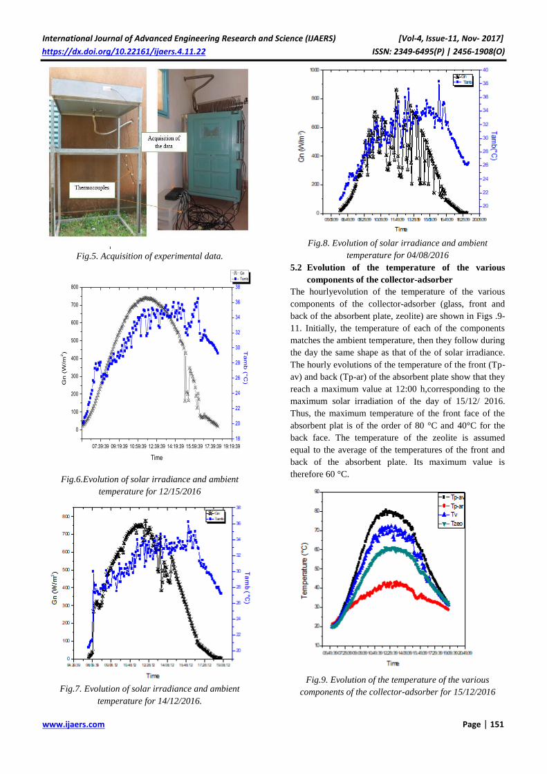
International Journal of Advanced Engineering Research and Science (IJAERS) [Vol-4, Issue-11, Nov- 2017]

https://dx.doi.org/10.22161/ijaers.4.11.22 ISSN: 2349-6495(P) | 2456-1908(O)

www.ijaers.com Page | 151

Fig.5. Acquisition of experimental data.

07:39:39 09:19:39 10:59:39 12:39:39 14:19:39 15:59:39 17:39:39 19:19:39

0

100

200

300

400

500

600

700

800

Gn

Tamb

Time

Gn

(W

/m2)

18

20

22

24

26

28

30

32

34

36

38

Ta

mb

(°C

)

Fig.6.Evolution of solar irradiance and ambient

temperature for 12/15/2016

Fig.7. Evolution of solar irradiance and ambient

temperature for 14/12/2016.

Fig.8. Evolution of solar irradiance and ambient

temperature for 04/08/2016

5.2 Evolution of the temperature of the various

components of the collector-adsorber

The hourlyevolution of the temperature of the various

components of the collector-adsorber (glass, front and

back of the absorbent plate, zeolite) are shown in Figs .9-

11. Initially, the temperature of each of the components

matches the ambient temperature, then they follow during

the day the same shape as that of the of solar irradiance.

The hourly evolutions of the temperature of the front (Tp-

av) and back (Tp-ar) of the absorbent plate show that they

reach a maximum value at 12:00 h,corresponding to the

maximum solar irradiation of the day of 15/12/ 2016.

Thus, the maximum temperature of the front face of the

absorbent plat is of the order of 80 °C and 40°C for the

back face. The temperature of the zeolite is assumed

equal to the average of the temperatures of the front and

back of the absorbent plate. Its maximum value is

therefore 60 °C.

Fig.9. Evolution of the temperature of the various

components of the collector-adsorber for 15/12/2016

International Journal of Advanced Engineering Research and Science (IJAERS) [Vol-4, Issue-11, Nov- 2017]

https://dx.doi.org/10.22161/ijaers.4.11.22 ISSN: 2349-6495(P) | 2456-1908(O)

www.ijaers.com Page | 152

Fig.10.Hourly evolution of the temperature of the various

components of the collector-adsorber during the day of

14/12/2016

Fig.11. Evolution of the temperature of the various

components of the collector-adsorber for 04/08/2016

5.3 Evolution of the condenser temperature

Figs. 12-14 show the hourlyevolution of the condenser

temperature during the different days of experimentation.

It should be noted that the temperature of the condenser is

equal to the ambient temperature up to 9h. Then, it

gradually increases over time until the maximum

difference with the ambient temperature is equal to 17 ° C

(15/12/2016). This increase of the temperature results

mainly from the amount of heat released during the water

vapor condensation on the walls of the condenser. The

amount of water vapor desorbed is all the more important

that the difference between the temperature of the

condenser and that of the ambient is large. After 12:00 h,

the temperature of the condenser decreases along with the

reduction of solar irradiance. It follows that the flow rate

of the desorbed water vapor decreases with time, which

causes a decrease in the temperature of the condenser. At

approximately 16:00 h, the hourly evolution of the

condenser temperature is similar to that of the ambient

temperature.

Fig.12 Evolution of the condenser and ambient

temperature for 15/12/2016

05:09:3906:49:3908:29:3910:09:3911:49:3913:29:3915:09:3916:49:3918:29:39

20

25

30

35

40

45

50

Te

mp

era

ture

(°C

)

Time

Tcd

Tamb

Fig.13 Evolution of the condenser and ambient

temperature for 14/12/2016

International Journal of Advanced Engineering Research and Science (IJAERS) [Vol-4, Issue-11, Nov- 2017]

https://dx.doi.org/10.22161/ijaers.4.11.22 ISSN: 2349-6495(P) | 2456-1908(O)

www.ijaers.com Page | 153

Fig.14 Evolution of the condenser and ambient

temperature for 04/08/2016

5.4 Evolution of the evaporator and the storage tank

temperature

We have shown in Fig. 15-17 the hourly evolution of the

evaporator (Tev) and the storage tank (Tst) temperatures.

We note that the hourly evolution for these two

temperatures, during the test days, is similar between

18:00 h to 6:00 h. During this period, the amount of cold

is produced by the evaporation of water at low pressure.

The high adsorption capacity of the zeolite makes it

possible to adsorb large amounts of water vapor, which

allows the continuation of the vaporization of the water

and thus the production of cold in the refrigerating

enclosure.

The evaporator tempearture and that of the storage tank

begin to decrease from 18:00 h until reaching a

temperature about +4°C at about 6:00 h. However, during

the day, the evaporator tempearture and that of the storage

tank gradually increase until reaching maximum values of

22°C (14/12/2016). This increase of the temperature is

partly due to the infiltration of air into the refrigerating

enclosure and also the energy losses and the climatic

conditions.

Fig.15 Evolution of the evaporator and the storage tank

temperatures for 14/12/2016

Fig.16 Evolution of the evaporator and the storage tank

temperatures for 15/12/2016

Fig.17 Evolution of the evaporator and the storage tank

temperatures for 04/08/2016

International Journal of Advanced Engineering Research and Science (IJAERS) [Vol-4, Issue-11, Nov- 2017]

https://dx.doi.org/10.22161/ijaers.4.11.22 ISSN: 2349-6495(P) | 2456-1908(O)

www.ijaers.com Page | 154

VI. PERFORMANCE OF ADSORPTION

REFRIGERATION SYSTEM

The thermal performance of the solar adsorption

refrigerator is characterized by the solar performance

coefficient (SCOP). This coefficient is the ratio between

the amount of the cooling production to the heat input

more precisely the total solar energy captured by the

collector-adsorber during a day.

. .ss

sr

f

t

s

t

QSCOP

A Gn dt

(3.1)

Where As is the collecting surface and Gn is the solar

irradiation

fQ is the amount of cold product at the evaporator :

.f ad l cd evQ m L Tev Cp T T (3.2)

The prototype that we have experimented is not equipped

with a device for measuring the cycled condensate mass

during a cycle of operation of the solar adsorption

refrigerator. This quantity is an important parameter

because it allows the calculation of the amount of cold

fQ produced at the evaporator. Thus, we used the

correlation of Errougani, A. (2007) [19] to estimate the

mass of cycled condensate (adm ) as a function of the

ambient temperature and the incident daily solar

irradiation. This correlation is given by equation (3.3):

log 2, 44859*log 4,0886ad

Gnm

Tamb

(3.3)

Where Gn is kJ / m2 and Tamb in (K).

Table 3.1 gives the solar performance coefficient (SCOP)

estimates for the different days of experimentation. The

experimental SCOP of our solar adsorption refrigeration

system varies between 0.09 to 0.185 and the total energy

received by the adsorber-collector varies between 15 and

19 MJ. The low SCOP value obtained can be explained

by the small amount of cold produced due to the small

amount of adsorbed refrigerant compared to the solar

thermal energy received by the adsorber collector.

Table.1: Coefficient of performance of the solar adsorption refrigerator.

Day

Solar radiation

energy (MJ)

Amount of cold

produced(MJ)

Evaporator

temperature (°C)

Condenser

temperature (°C)

SCOP

Max Min Max Min

03/08/2016 15,519 1,40 16 11 47 26 0,09

04/08/2016 21,86 2,21 14 9,5 44 28 0,101

05/08/2016 18,15 1.87 18 8 42 25 0,103

11/12/2016 15,77 2,69 16 11 47 26 0,171

12/12/2016 15,12 2,40 14 9,5 44 28 0,158

13/12/2016 19.66 3.30 18 8 42 25 0,167

14/12/2016 21,32 3,78 21 12 45 21 0,177

15/12/2016 19,60 3,63 15 4 52 20 0,185

16/12/2016 19,66 3,30 16 6 49 23 0,167

Table.2: Comparison SCOP of some solar refrigerator adsorption system

adsorbent/adsorbate SCOP Total energy received

Present experimental study Zeolithe/water 0.09-0.185 15-20 MJ/m2

Hildbrand et al. (2004) Silicagel/ water 0.12-0.23 > 20 MJ/m2.

Philippe Dind et al. (2005) Silicagel/ water 0.19 Artificial sunshine

A.Boubakri et al. (1992) AC/methanol 0.12 19.54 MJ/m2

Hildbrand et al. (2005) AC/methanol 0.09-0.13 19-25 J/m2

We compared the obtainedresults with those of the

literature (Table 3.2). We found that these values are of

the same order of magnitude as in the literature [16-18]

using the zeolite-water or silica gel-water pair. This

validates our experimental protocol and demonstrates the

technical feasibility of the solar adsorption refrigerator

prototype that we used.

VII. CONCLUSION

In this paper, an experimental solar adsorption

refrigerator, using the zeolite/water pair, is presented.

International Journal of Advanced Engineering Research and Science (IJAERS) [Vol-4, Issue-11, Nov- 2017]

https://dx.doi.org/10.22161/ijaers.4.11.22 ISSN: 2349-6495(P) | 2456-1908(O)

www.ijaers.com Page | 155

Designed for the conservation of pharmaceutical

products, several experimental tests have been carried out

in order to test the reliability of the solar adsorption

refrigeration system. Thus, the hourly evolution of the

temperature of the different components of the system

was presented and discussed:

The maximum value of solar irradiance varies

between 750 and 830 W / m2. Tthe maximum value

of the recorded ambient temperature was

approximately 38 °C and the minimum value was 21

°C.

The maximum temperature of the front face of the

absorbent plat is of the order of 80 °C and that of the

back face is 40°C. The temperature of the zeolite is

maximum value is therefore 60 °C.

The temperature of the condenser reaches a

maximum temperature of 52 °C and that of the

evaporator, a minimum temperature of 4 °C.

The SCOP of the solar adsorption refrigeration system

varies between 0.09 to 0.185 and the total energy received

by the adsorber-collector varies between 15 and 19 MJ.

Acknowledgements

The authors are grateful to the University Agency of the

Francophonie (AUF) and the French Embassy (SCAC)

for financial support which allowed the realization of this

work.

Nomenclature

Cp Specific heat (J/kg.K)

Gn Solar radiation (W/m2)

m mass (kg)

Qf Cold production (J)

q Water concentration inside the

zéolithe (kg/kg)

A Area (m2)

L(T) Latent heat of vaporization (J/kg)

T Température (K)

P Pressure (Pa)

Indexes

amb ambient

zeo zeolite

ev evaporator

cd condenser

v glass

p plaque

st storage

t Time (s)

g generation

ad adsorbent

REFERENCES

[1] Ousmane, M., Dianda, B., Kam, S., Konfe, A., Ky,

T. and Bathiebo, D. (2015) Experimental Study in

Natural Convection. Global Journal of Pure and

Applied Sciences, 21, 155-169.

https://doi.org/10.4314/gjpas.v21i2.8

[2] A. Chikouche, «Using solar energy for refrigeration

purposes in Algeria,» chez 4th JIIRCRAC

Proceeding, 2012.

[3] Marlinda, A. Uyun, T. Miyazaki, Y. Ueda et A.

Akisawa, « Performance analysis of a double-effect

adsorption refrigeration cycle with a silica gel/water

working pair,» Energies, pp. 3,1704–1720., 2010.

[4] Tubreoumya, G.C., Dissa, A.O., Tiendrebeogo, E.S.,

Chesneau, X., Compaore, A., Haro, K., Konseibo,

C.D., Zeghmati, B. and Koulidiati, J. (2017)

Contribution to the Modeling of a Solar Adsorption

Refrigerator under the Climatic Conditions of

Burkina Faso. Energy and PowerEngineering, 9,

119-135. https://doi.org/10.4236/epe.2017.92010

[5] Allouhi, A., Kousksou, T., Jamil, A. and Zeraouli,

Y. (2014) Modeling of a ThermalAdsorber Powered

by Solar Energy for Refrigeration Applications.

Energy, 75, 589-596.

https://doi.org/10.1016/j.energy.2014.08.022

[6] H. Hassan, A. Mohamad et H. Al-Ansary,

Development of a continuously operating solar-

driven adsorption cooling system: Thermodynamic

analysis and parametric study. Appl. Therm. Eng, pp.

48, 332–341, 2012.

http://dx.doi.org/10.1016/j.applthermaleng.2012.04.

040

[7] Boubakri, A., Guilleminot, J. and Meunier, F. (2000)

Adsorptive Solar Powered Ice Maker: Experiments

and Model. Solar Energy, 69, 249-263.

https://doi.org/10.1016/S0038-092X(00)00063-3

[8] Lemmini, F. and Errougani, A. (2007)

Experimentation of a Solar Adsorption Refrigerator

in Morocco. Renewable Energy, 32, 2629-2641.

https://doi.org/10.1016/j.renene.2007.01.004

[9] M. Louajari, A. Mimet et A. Ouammi, «Study of the

effect of finned tube adsorber on theperformance of

solar driven adsorption cooling machine using

activated carbon-ammonia pair.»Appl. Energy , pp.

88, 690–698., 2011.

http://dx.doi.org/10.1016/j.apenergy.2010.08.032

[10] Muhammad, U., Atsushi, A. and Yuki, U. (2014)

Performance Evaluation of a SolarAdsorption

Refrigeration System with a Wing Type Compound

Parabolic Concentrator. Energies, 7, 1448-1466.

https://doi.org/10.3390/en7031448

[11] Bakkas, M., Mada, M. and Tahri, M. (2001)

Modelisation et Simulation du Transfert de Chaleur

et de Masse a l'Interieur d'un Reacteur de Charbon

Actif Reagissant avec de l’Ammoniac Couple a un

Caloduc Annulaire a Eau. Revue des Energies

Renouvelables, 19-24.

International Journal of Advanced Engineering Research and Science (IJAERS) [Vol-4, Issue-11, Nov- 2017]

https://dx.doi.org/10.22161/ijaers.4.11.22 ISSN: 2349-6495(P) | 2456-1908(O)

www.ijaers.com Page | 156

[12] Allouhi, A., Kousksou, T., Jamil, A., El Rhafiki, T.,

Mourad, Y. and Zeraouli, Y.(2015) Optimal

Working Pairs for Solar Adsorption Cooling

Applications. Energy,79, 235-247.

https://doi.org/10.1016/j.energy.2014.11.010

[13] Leite, A.D.M. (2000) Performance of a New Solid

Adsorption Ice Maker with SolarEnergy

Regeneration. Energy Conversion and Management,

41, 1625-1647.

https://doi.org/10.1016/S0196-8904(00)00011-X

[14] Guilleminot, J.M.F. (1987) Heat and Mass Transfer

in a Non Isothermal Fixed BedSolid Adsorbent

Reactor a Uniform Pressure-Non Uniform

Temperature. International Journal of Heat and Mass

Transfer, 30, 1595-1606.

https://doi.org/10.1016/0017-9310(87)90304-8

[15] Mimet, A. (1991) Etude theorique et experimentale

d’une machine frigorifique a adsorption d’ammoniac

sur charbon actif. These de Doctorat, FPMs, Mons.

[16] Boubakri, A., Arsalane, M., Yous, B., Alimoussa,

L., Pons, M., Meunier, F., Guilleminot, J. (1992).

Experimental study of adsorptive solar powered ice

makers in Agadir (Morocco)-1.Performance in

actual site. Renew. Energ.(2 (1), 7-13.), 2 (1), 7-13.

[17] Dind, P., Catherine., H., Cherbuin, O., Mayor, J.

(2005). La réfrigération solaire à adsorption. HES-

SO: Projet Gerbert Rüf Stiftung.

[18] Hildbrand, C., Dind, P., Pons, M., Buchter, F.

(2004). A new solar powerd adsorption refrigerator

with high performance. Solar Energy, vol 77,

pp.311-

318https://doi.org/10.1016/j.solener.2004.05.007

[19] Errougani, A. (2007). Fabrication et experimentation

d’un refrigerateur solaire a adsorption utilisant le

couple charbon actif- methanol. Agdal: Université

Mohammed V.

International Journal of Advanced Engineering Research and Science (IJAERS) [Vol-4, Issue-11, Nov- 2017]

https://dx.doi.org/10.22161/ijaers.4.11.23 ISSN: 2349-6495(P) | 2456-1908(O)

www.ijaers.com Page | 157

General Pattern Search Applied to the

Optimization of the Shell and Tube Heat

Exchanger Wagner H. Saldanha, Pedro A. A. M. Junior

Department of Mechanical Engineering, Pontifícia Universidade Católica de Minas Gerais, Belo Horizonte, Brasil

Abstract— The literature has different implementations

and results for the mono-objective and multiobjective

optimization of the shell and tube heat exchanger (STHE),

most of them using evolutionary computation. However,

there is a gap to find the optimal solution of this problem

through direct search methods (numerical optimization).

So, this paper uses the Pattern Search algorithm of

MATLAB toolbox applied to this case study.

Keywords— Optimization, Pattern Search algorithm,

Shell and Tube Heat Exchanger.

I. INTRODUCTION

Heat exchangers are used in process industries, steam

generating plants, refrigeration systems, heating systems,

air conditioning, petrochemical industries, among other

applications. Its function is to provide the recovery and

use of thermal energy efficiently and economically. There

are different models of heat exchangers, such as spiral,

plates, regenerators, compacts, shell and tube heat

exchanger (STHE). During its design it is possible to

obtain different configurations, however, it is desirable

the optimal design, which starts from the modeling of the

same.

The recent literature review [1] shows the trend in the use

of Evolutionary Algorithms for the mono-objective

optimization of STHE. The most commonly used

technique is Genetic Algorithm (GA). Other algorithms

are Particle Swarm Optimization (PSO), Harmony Search

Algorithm, Differential Evolution, Cuckoo Search

Algorithm, Imperialist Competitive Algorithm,

Biogeography Base Algorithm, Simulated Annealing,

Firefly algorithm, Bat Algorithm, and Jaya algorithm. In

the multiobjective optimization are the Non-Dominated

Sorting Genetic Algorithm II (NSGA II) and the Multi-

Objective Particle Swarm Optimizer (MOPSO).

Considering the previous discussion, the objective of this

article is to solve the mono-objective optimization of the

STHE by minimizing the objective function total annual

cost with the use of the algorithm General Pattern Search

(GPS), which is implemented in the MATLAB toolbox.

II. OPTIMIZATION OF THE SHELL AND TUBE

HEAT EXCHANGER

The problem considered is the minimization of the total

annual cost (TC) of the shell and tube heat exchanger.

Min f(x), f(x) =TC, (1)

The modeling and problem of the shell and tube heat

exchange used in this article are the found in [1-3]. The

variables used for the multiobjective optimization are

presented in Table 1.

Table.1: Variables for optimization of the Shell and Tube

Heat Exchanger

Var. Symbol Values

x1 ap

triang. (30º); square (90º); rot. square

(45º)

x2 np 1; 2; 4

x3 Lt 2.438 m to 11.58 m

x4 esp 0.002108 m to 0.004572 m

x5 do 0.01588 m to 0.0508 m

x6 Lb 0.0508 m to 29.5(x5)0.75

x7 bc 15% to 45%

x8 dtb 0.01x5 to 0.1x5

x9 dsb 0.0032 m to 0.011 m

Follow the description of the variables: ap is the tube

layout pattern, np is the number of tubes passes, Lt is the

tube length, esp is the tube wall thickness, do is the tube

outer diameter, Lb is the baffle spacing, bc is the baffle

cut, dtb is the tube-to-baffle diametrical clearance, dsb is

the shell-to-baffle diametrical clearance.

Considering the material of the tube (70%Cu, 30%Ni)

and of the shell (carbon steel), the total anual cost

estimation )(TC that includes direct and indirect costs

)( BMC and operational costs )(OC , was conducted in

the same manner as in [1,2]:

OCi

iiCTC

n

n

BM

1)1(

)1( (2)

Where i is the fractional interest rate per year, n is the

lifetime in years estimated for the heat exchanger. Being

that the operational costs are in function of the pressure

International Journal of Advanced Engineering Research and Science (IJAERS) [Vol-4, Issue-11, Nov- 2017]

https://dx.doi.org/10.22161/ijaers.4.11.23 ISSN: 2349-6495(P) | 2456-1908(O)

www.ijaers.com Page | 158

drop, and direct and indirect costs are in function of the

thermal exchange area.

Three constraints was considered involve the limits of the

shell side pressure drop, the tube side pressure drop, and

the maximum área value of the heat exchanger. The

formulation was the same as the one considered in [1,3,4].

III. EXPERIMENTS AND RESULTS

The optimization of shell and tube heat exchanger was

performed by direct search [5,6], through the Pattern

Search algorithm of the MATLAB toolbox, and the

configuration of the Poll and Search methods used was

the General Pattern Search positive basis 2N (GPS) [7-

9], the other settings were the program standards.

The result obtained by the GPS was compared to the

multiobjective optimization performed by the algorithm

NSGA II and transformed to the minimum annual cost

criterion used in [1]. The GPS algorithm was also

compared to the result found for the genetic algorithm of

MATLAB toolbox. In this case, a configuration used was

50 generations, uniform stochastic selection, scattered

crossover, and mutation constraint dependent.

The Table 2 and Table 3 show the best results found for

algorithm GPS. In Table 4 the results for the GA

algorithm are presented and in Table 5 has the results for

NSGA II algorithm.

Table.2: Results for optimization, GPS algorithm,

triangular tube arrangement, one tube pass

Variable Value

ap Triangular

np 1

Lt 2,438 m

esp 0,002108 m

do 0,01588 m

Lb 0,9925 m

bc 17,4 %

dtb 0,0001588 m

dsb 0,0032 m

Function objective Value

$ 3335,45

Table.3: Results for optimization, GPS algorithm, rotated

square tube arrangement, one tube pass

Variable Value

ap rotated square

np 1

Lt 2,438 m

esp 0,002352 m

do 0,01863 m

Lb 0,711 m

bc 15,3 %

dtb 0,0001588 m

dsb 0,0032 m

Function objective Value

$ 3346,77

Table.4: Results for optimization, GA algorithm

Variable Value

ap rotated square

np 1

Lt 3,658 m

esp 0,002108 m

do 0,01905 m

Lb 0,8588 m

bc 18,6 %

dtb 0,0003921 m

dsb 0,0054 m

Function objective Value

$ 3362,45

Table.5: Results for optimization, NSGA II algorithm

Variable Value

ap Triangular

np 1

Lt 2,438 m

esp 0,002108 m

do 0,01588 m

Lb 1,6312 m

bc 17,4 %

dtb 0,0004775 m

dsb 0,0042 m

Function objective Value

$ 3337,12

For the triangular tube arrangement configuration and one

tube pass, the result was better than the obtained by the

algorithm NSGA II. And for the arrangement square

rotated and one tube pass the algorithm also obtained

better performance than the GA.

During the experiment, GPS algorithm was applied for all

combinations of discrete variables of the STHE, so nine

results were obtained. However, it was chosen to present

only the best results and that could be compared to other

optimization algorithms.

It is understood that the configuration of the STHE with

square tube arrangement, rotated square tube arrangement

with two tube passes or four tube passes, and triangular

tube arrangement with two tube passes or four tube

passes, does not allow good results.

IV. CONCLUSION

The GPS algorithm was a viable alternative for the mono-

objective optimization of the shell and tubes heat

exchanger, being that it found better results than the

International Journal of Advanced Engineering Research and Science (IJAERS) [Vol-4, Issue-11, Nov- 2017]

https://dx.doi.org/10.22161/ijaers.4.11.23 ISSN: 2349-6495(P) | 2456-1908(O)

www.ijaers.com Page | 159

popular algorithms like NSGA II and GA.

This result is important and interesting because most

paper that apply optimization of the heat exchanger use

heuristic methods, especially with the use of genetic

algorithm (GA). However, when a competitive result is

found with a direct search algorithm, one must extend the

use of numerical optimization applied to other real

problems. In addition, it is suggested that it encourages its

use in hybrid algorithms.

REFERENCES

[1] Saldanha, W. H. et al., (2017). Choosing the best

evolutionary algorithm to optimize the multiobjective

shell and tube heat exchanger design problem using

PROMETHEE. Applied Thermal Engineering, vol.

127, pp. 1049-1061.

[2] Fettaka, S.; Thibault, J.; Gupta, Y., (2013). Design of

shell and tube heat exchangers using multiobjective

optimization. International Journal of Heat and Mass

Transfer, vol. 60, n. 1, pp. 343-354.

[3] Shah, R. K.; Sekulic, D. P., (2003). Fundamentals of

heat exchanger design. John Wiley Sons

[4] Wildi-Tremblay, P. and Gosselin, L., (2007).

Minimizing shell and tube heat exchanger cost with

genetic algorithms and considering maintenance.

International Journal of Energy Research, vol. 31, n.

9, pp. 867-885.

[5] Hooke, R. and Jeeves, T. A., (1961). Direct search

solution of numerical and statistical problems.

Journal of the ACM, vol. 8, n. 2, pp. 212-229.

[6] Kolda, T. G.; Lewis, R. M.; Torczon, V., (2003).

Optimization by direct search: new perspectives on

some classical and modern methods. SIAM review,

vol. 45, n. 3, pp. 385-482.

[7] Torczon, V., (1997). On the convergence of pattern

search algorithms. Journal on Optimization, vol. 7,

pp. 1-25.

[8] Lewis, R, M.; Torczon, V., (1997). Pattern search

algorithms for bound constrained minimization.

SIAM Journal on Optimization, vol. 9, n. 4, pp.

1082-1099.

[9] Audet, C.; JR, J.E.D., (2002). Analysis of generalized

pattern searches. SIAM Journal on optimization, vol.

13, n. 3, pp. 889-903.

International Journal of Advanced Engineering Research and Science (IJAERS) [Vol-4, Issue-11, Nov- 2017]

https://dx.doi.org/10.22161/ijaers.4.11.24 ISSN: 2349-6495(P) | 2456-1908(O)

www.ijaers.com Page | 160

Study the Dynamic Response of the Stiffened

Shallow Shell Subjected to Multiple Layers of

Shock Waves Le Xuan Thuy

Department of Solid Mechanics, Le Quy Don Technical University, Ha Noi, Viet Nam

Abstract— The ANSYS APDL programming and the

results of calculating the stiffened shallow shell on elastic

supports subjected to multiple layers of shock waves

presented in the study. The program set up allows for the

survey and evaluation of structural parameter and loads

to the dynamic response of different types of shallow

shell.

Keywords— Dynamic, Shell, shock wave, Elastic

supports.

I. INTRODUCTION

The shell is used in many areas due to its good coverage

and light weight. Some structures can be mentioned as:

roof of the building, cover tunnel, engine cover, …

Calculation of shell structure is influenced by different

types of load are many scientists concerned. One of the

types of high destructive load mentioned is the shock

wave load [1,2,3,4,5]. In fact, when exposed to multiple

layers of shock waves, the structural response is complex.

To avoid the impact of impulse load, in some cases the

elastic supports is used. In this paper, the problem of

shallow shell structure with (or without) elastic supports

subjected to multi layers of shock waves is investigated.

The study results may give the readers a more complete

vision on the response of the mentioned shell structure

and may be used for reference in the its design.

II. PROBLEM MODELING

The Considering an eccentrically stiffened singly (or

doubly) curved shell that is simply supported at the edges

by elastic springs with stiffness k (Fig. 1). The shell is

affected by multiple layers of shock waves p(t).

y

x

z

p(t)

Fig. 1: Problem Model

For establishing an algorithm for the problem the

following assumptions are used:

- The ribs and the shell material are homogeneous

and isotropic;

- The shock-wave presssure is uniformly

distributed on the shell surface.

III. TYPES OF ELEMENTS USED IN THE

PROGRAM

To describe the bending shell, the SHELL63 element is

used. The element has six degrees of freedom at each node:

translations in the nodal x, y, and z directions and rotations

about the nodal x, y, and z-axes. Stress stiffening and large

deflection capabilities are included [8].

Fig. 2: SHELL63 Geometry

To describe the stiffener, 3-D Linear Finite Strain Beam

(BEAM188) is used. BEAM188 is a linear (2-node) or a

quadratic beam element in 3-D. It has six or seven

degrees of freedom at each node, with the number of

degrees of freedom depending on the value of

KEYOPT(1). When KEYOPT(1) = 0 (the default), six

degrees of freedom occur at each node. The eccentricity

of the stiffener is described by the SECOFFSET

command [8].

Fig. 3: BEAM188 Geometry

Elastic springs are described by the COMBIN14 element.

With this type of element, the computational power of the

International Journal of Advanced Engineering Research and Science (IJAERS) [Vol-4, Issue-11, Nov- 2017]

https://dx.doi.org/10.22161/ijaers.4.11.24 ISSN: 2349-6495(P) | 2456-1908(O)

www.ijaers.com Page | 161

program is extended to other types of viscoelastic pillows.

In this case, the damping coefficient should be added

when declaring the constants of the COMBIN14 element.

Fig. 4: COMBIN14 Geometry [8]

COMBIN14 has longitudinal or torsional capability in 1-

D, 2-D, or 3-D applications. The longitudinal spring-

damper option is a uniaxial tension-compression element

with up to three degrees of freedom at each node:

translations in the nodal x, y, and z directions. No

bending or torsion is considered. The torsional spring-

damper option is a purely rotational element with three

degrees of freedom at each node: rotations about the

nodal x, y, and z axes. No bending or axial loads are

considered [8].

IV. GOVERNING EQUATIONS AND

CALCULATION PROGRAM

The connection of the rib and the support elements into

the flat shell elements is implemented by the direct

stiffness method and the Skyline diagram is established

by using the general algorithm of the FEM [6, 7, 8].

After connecting the element matrices and the element

vectors in to the global ones the differential equation

describing the oscillation of the stiffened shell may be

written in the form:

M q + q + q = F ,C K (*)

where:

e e

s b

e e

M = M + M - the overall mass matrix ( s

eM

- the element mass matrix of shell element,

ebM - the

element mass matrix of beam element);

e e e

s b sp

e e e

K = K + K + K - the overall stiffness

matrix ( s

eK ,

ebK ,

espK - the element stiffness matrix

of shell element, beam element and combin14 element

respectively);

e es b

e e

F = F + F - the overall load vector;

R RC = a M +b K - the overall damping matrix, where

αR, βR are Rayleigh damping coefficients [7,8].

Solution of equation (*) provided by the algorithm of

calculator in ANSYS software. Depending on the choice

of linear or nonlinear solvers, the Newmark’s direct

integration algorithm is used or combined using the

Newton-Raphson iteration method.

A program to calculate the stiffened shallow shell subjected

to multiple layers of shock waves on ANSYS APDL

language written called Shallow_shell_multishock_waves

(SSMW). The program includes the following modules:

- Modul 1: Import_data.mac;

- Modul 2: Model_building.mac;

- Modul 3: Loading_and_solving.mac;

- Modul 4: Export_ result.mac.

Within the scope of the study, the calculation program was

designed to calculate two types of shell: shallow

cylindrycal shell and doubly curved shell.

V. NUMERICAL RESULTS AND

DISCUSSION

1. Problem 1

Consider an eccentrically stiffened shallow cylindrical

shell whose plan view is a rectangular, a = 2.0m, b =

1.0m, the radius of curvature R = 1.6m, the thickness h =

0.025m. Shell material has an elastic modulus Es =

2.11011N/m2, poisson coefficient s = 0.3, specific

weight s = 7850kg/m3. Four edges of shell are supported

by elastic springs with stiffness k = 3.104 kN/m. The

eccentric ribs of the shell has hr = 0.03m, br = 0.01m, the

ribs in the directions are 6 (6 ribs parallel to the

generating line, 6 ribs perpendicular to the generating

line). The ribbed material has Er = 2.51011N/m2, r = 0.3,

r = 7500kg/m3.

yx

z

P(t)

I

Z

Y

a/6

hg

bg

h

I

a

a/12

shellRib

Fig. 5: Model of problem 1

The working load is two shock waves acting on the shell

maxp t p F t , with: pmax1 = pmax2 = 3.104 N/m2,

t

1 : 0 tF t

0 : t

, τ1 = τ2 = 0.05s, time difference

between wave layers: Δτ = 0.02s.

International Journal of Advanced Engineering Research and Science (IJAERS) [Vol-4, Issue-11, Nov- 2017]

https://dx.doi.org/10.22161/ijaers.4.11.24 ISSN: 2349-6495(P) | 2456-1908(O)

www.ijaers.com Page | 162

pmax

p

tΔτ

τ1

Fig. 6: Variation law of the load

Using the SSMW program, the author solved the problem

with the calculating time tcal = 0.16s, integral time step

Δt =0.0005s. Resulting in stress and vertical displacement

at the center of the shell, as shown in Table 1 and Figures

7, 8, 9.

Table.1: The maximum value of the quantity calculated in

problem 1

wmax [cm] max

x [N/m2] max

y [N/m2]

SSMW 0.0115 3.5977106 1.5273106

Fig. 7: Vertical displacement response w at center point

Fig. 8: Stress response σx, σy at center point

Fig. 9: Field of von mises stress of the shell at time t = 0.021s

Comment: With the given set of data, the maximum

dynamic response values of the system reached at the

time of two waves of simultaneous effects (time t =

0.021s). At center point, the stress σxmax is greater than the

stress σymax.

2. Problem 2

Considering the shallow cylindrical shell whose plan

view is a rectangular, generating line’s length a = 2.0m,

opening angle of the shell θ = 40o, the radius of curvature

is R = 2.0m, h = 0.02m, Es = 2.21011N/m2, s = 0.31, s

= 7800kg/m3. The eccentrically ribbed shell with hr =

0.03m, br = 0.01m, the shell with 4 ribs is parallel to the

generating line, 6 ribs is perpendicular to the generating

line, the ribs are equispaced. Er = 2.41011N/m2,

r = 0.3, r = 7000kg/m3. The mentioned shell has a round

hole in the middle position, with d = 0.2 m (fig. 10). The

load acting and the boundary are the same as Problem 1.

Vertical displacement and stress at point A, field of von

mises stress of the shell and the overall transposition field

of the structure at time t = 0.021s are shown in Figure 11,

12, 13, 14 and table 2.

yx

z

A

Fig. 10: Model of problem 2

Table.2: The maximum value of the quantity calculated in

problem 2

wAmax[cm] Amax

x [N/m2] Amax

y [N/m2]

SSMW 0.0178 24.502106 3.669106

Fig. 11: Vertical displacement response w at point A

International Journal of Advanced Engineering Research and Science (IJAERS) [Vol-4, Issue-11, Nov- 2017]

https://dx.doi.org/10.22161/ijaers.4.11.24 ISSN: 2349-6495(P) | 2456-1908(O)

www.ijaers.com Page | 163

Fig. 12: Stress response σx, σy at point A

Fig. 13: Field of von mises stress of the shell at time t = 0.021s

Fig. 14: The overall transposition field of the structure

at time t = 0.021s

Comment: Immediately after the second wave appeared,

the vertical displacement of the point A increases quite a

lot, which represents the great influence of the second

wave on the structure. At the time t = 0.021s, the shell

appeared four symmetrical areas through the center with

relatively large stress and displacement responses

compared to the other positions. This is due to the

reduction in the pressure applied to the position at the

center of the cover.

3. Problem 3

Considering the doubly curved shell whose plan view is a

rectangular, a = 1.5m, b = 1.0m, R1 = 2.0m, R2 = -4.0m,

the thickness h = 0.005m. Shell material has Es = 2.11011

N/m2, s = 0.31, s = 7800kg/m3 (fig. 15). The load acting

is the same as Problem 1.

Vertical displacement and stress at center point, field of

von mises stress of the shell and the overall transposition

field of the structure at time t = 0.025s are shown in

Figure 16, 17, 18, 19 and table 3.

b

a

R1R2

x y

z

Fig. 15: Model of problem 3

Fig. 16: Vertical displacement response w at center point

Fig. 17: Stress response σx, σy at center point

Fig. 18: Field of von mises stress of the shell at time t = 0.025s

International Journal of Advanced Engineering Research and Science (IJAERS) [Vol-4, Issue-11, Nov- 2017]

https://dx.doi.org/10.22161/ijaers.4.11.24 ISSN: 2349-6495(P) | 2456-1908(O)

www.ijaers.com Page | 164

Fig. 19: The overall transposition field of the structure

at time t = 0.025s

Table.3: The maximum value of the quantity calculated in

problem 3

wmax[cm] max

x [N/m2] max

y [N/m2]

SSMW 0.0204 49.535106 42.782106

Comment: Like the results of the problem 1 and problem

2, the maximum dynamic response values at point A of

the structure reached at the time of two waves of

simultaneous effects.

4. Problem 4

The parameters of the model are similar to the parameters

in problem 3. The difference is that the shell has a square

hole (a1 x a1) in the middle position, with a1 = 0.2 m.

Table.4: The maximum value of the quantity calculated in

problem 4

wAmax[cm] Amax

x [N/m2] Amax

y [N/m2]

SSMW 0.0126 7.348106 71.405106

b

a

R1

R2

x y

z a1A

Fig. 20: Model of problem 4

Fig. 21: Vertical displacement response w at point A

Fig. 22: Stress response σx, σy at point A

Fig. 23: Field of von mises stress of the shell at time t = 0.01s

Fig. 24: The overall transposition field of the structure

at time t = 0.01s

Comment: Compared to the result at the midpoint of the

shell in Problem 3, the maximum value of the stress

response at point A (σymax) is much greater, this shows

that the more susceptible to damage of the structure when

there is a defect on its.

VI. CONCLUSION

In this study, using the ANSYS APDL programming

language, a program has been established that allows for

solving many different problem classes. The paper

focuses on solving the problem of calculating the shell

structure with one or two curvature with or without holes,

which is affected by the impulse load system. The results

show the complex response of the structure when multiple

layers of shock wave load are applied. Solving different

problem classes demonstrates the ability of the program.

International Journal of Advanced Engineering Research and Science (IJAERS) [Vol-4, Issue-11, Nov- 2017]

https://dx.doi.org/10.22161/ijaers.4.11.24 ISSN: 2349-6495(P) | 2456-1908(O)

www.ijaers.com Page | 165

The results of the study may be good references when

calculating, designing the same structural.

REFERENCES

[1] Ioannis G. Raftoyiannis, Constantine C. Spyrakos, George

T. Michaltsos (2007). Behavior of suspended roofs under

blast loading. Engineering Structures 29 (ISSN: 0141-

0296) 88–100, doi:10.1016/j.engstruct.2006.04.006.

[2] A. Ghani Razaqpur, Ahmed Tolba, Ettore

Contestabile (2007). Blast loading response of

reinforced concrete panels reinforced with externally

bonded GFRP laminates. Composites: Part B 38,

535–546, doi:10.1016/j.compositesb.2006.06.016.

[3] Zhenyu Xue, John W. Hutchinson (2003). Preliminary

assessment of sandwich plates subject to blast loads.

International Journal of Mechanical Sciences 45, 687–

705, doi:10.1016/S0020-7403(03)00108-5.

[4] H. S. Tӥrkmen (2002). Structural Response of

Laminated Composite Shells Subjected to Blast

Loading: Comparison of Experimental and Theoretical

Methods. Journal of Sound and Vibration 249(4), 663-

678, doi:10.1006/jsvi.2001.3861.

[5] Yonghui Wang, Ximei Zhai, Siew Chin Lee, Wei Wang

(2016). Responses of curved steel-concrete-steel sandwich

shells subjected to blast loading. Thin-Walled Structures

108, 185–192, http://dx.doi.org/10.1016/j.tws.2016.08.018.

[6] Saeed Moaveni (2008). Finite element analysis:

theory and application with ANSYS. Pearson

Prentice Hall., Pearson Education.Inc.

[7] Erdogan Madenci, Ibrahim Guven (2015). The finite

element method and applications in engineering

using ANSYS. Springer International Publishing.

[8] Release 11.0 Documentation for ANSYS.

International Journal of Advanced Engineering Research and Science (IJAERS) [Vol-4, Issue-11, Nov- 2017]

https://dx.doi.org/10.22161/ijaers.4.11.25 ISSN: 2349-6495(P) | 2456-1908(O)

www.ijaers.com Page | 166

Theoretical investigation of series of

diazafluorene-functionalized TTFs by using

density functional method Tahar Abbaz1*, Amel Bendjeddou1, Didier Villemin2

1Laboratory of Aquatic and Terrestrial Ecosystems. Org. and Bioorg. Chem. Group, University of Mohamed-Cherif

Messaadia, Souk Ahras, 41000, Algeria 2Laboratory of Molecular and Thio-Organic Chemistry, UMR CNRS 6507, INC3M, FR 3038, Labex EMC3, ensicaen &

University of Caen, Caen 14050, France

Abstract— Quantum chemical calculations of energies,

geometrical structure and electronic parameters of

diazafluorene-functionalized TTFs 1-4 were carried out

by using density functional (DFT/B3LYP) method with 6-

31G(d,p) as basis set. Stability of the molecule arising

from hyper conjugative interactions, charge

delocalization has been analyzed using natural bond

orbital (NBO) analysis. The calculated HOMO and

LUMO energies show that chemical activity of the

molecule. The local reactivity descriptor analysis is

performed to find the reactive sites within molecule.

Keywords— Computational chemistry, Density

functional theory, Electronic structure, Quantum

chemical calculations

I. INTRODUCTION

The chemistry of heterocyclic compounds has a key role

in the discovery of new drugs. This study field have

gathered great attention over the past years, and a number

of paper constructed by experimental techniques and

theoretical methods have appeared in the literature.

Various compounds such as alkaloids, essential amino

acids, vitamins, hemoglobin, hormones, large number of

synthetic drugs and dyes contain heterocyclic ring

systems. There are large numbers of synthetic

heterocyclic compounds, like pyrimidine, pyridine,

pyrrole, pyrrolidine, diazafluorene, furan and thiophene.

Heterocyclic compounds exhibits wide range of synthetic

and biological activities, especially nitrogen and sulfur

containing heterocyclic moieties were found to be vital

for a number of biologically active compounds [1].

Density functional theory (DFT) has become the

dominant tool in chemistry and physics for calculations of

electronic structure as it demands less time for inclusion

of electron correlation. Detailed analysis on the

applicability of different methods of DFT has been

performed, particularly for equilibrium structure

properties of geometry, vibrational frequency, etc [2]. The

general conclusion from these studies was that DFT

methods, particularly with the use of nonlocal exchange-

correlation functions, can predict accurate equilibrium

structure properties. NBOs provide an accurate method

for studying intramolecular interactions and give an

efficient basis to investigate charge transfer or conjugative

interaction in various molecular systems [3]. Molecular

electrostatic potential (MEP) is used to map and

understand the dimeric sites within the molecules. MEP is

very much required for predicting structure–activity

relationship and drug–receptor interactions of

biomolecules.

The present work aims to investigate the molecular

structure, electronic and non-linear optical properties of

series of diazafluorene-functionalized TTFs 1-4 described

in literature [4] and to predict their activities, we give a

global study of the molecular geometry, natural bond

orbital (NBO) analysis, nonlinear optical (NLO)

properties, and chemical reactivity as HOMO-LUMO

energy gap, chemical hardness, chemical potential and

local reactivity descriptors.

II. MATERIALS AND METHODS

All parameters and properties of diazafluorene-

functionalized TTFs 1-4 were calculated using the

Gaussian 09 software package on a personal computer

[5]. The computations were performed at B3LYP/6-

31G(d,p) level of theory to get the optimized geometries

shown in Fig 1 of the title compound. DFT calculations

were carried out with Becke’s three-parameter hybrid

model using the Lee-Yang-Parr correlation functional

(B3LYP) method.

III. RESULTS AND DISCUSSION

3.1. Molecular Geometry

The molecular structure along with numbering of atoms

of diazafluorene-functionalized TTFs molecules are as

shown in Fig 1.The calculated global minimum energy of

International Journal of Advanced Engineering Research and Science (IJAERS) [Vol-4, Issue-11, Nov- 2017]

https://dx.doi.org/10.22161/ijaers.4.11.25 ISSN: 2349-6495(P) | 2456-1908(O)

www.ijaers.com Page | 167

diazafluorene-functionalized TTFs 1-4 in C1 point group

symmetries are between -3189.3021and -4064.3090 a.u.

by 6-31G(d,p) basis set. The optimized bond lengths,

bond angles and dihedral angles of the title compound

which calculated using B3LYP method are with 6-

31G(d,p) basis set are shown in Tables 1-4.

Compound 1 Compound 2

Compound 3 Compound 4

Fig.1: Optimized molecular structure of diazafluorene-functionalized TTFs 1-4

Table.1: Optimized geometric parameters of compound 1

Bond Length(Å) Bond Angles (°) Dihedral Angles (°)

R(25,28) 1.082 A(27,24,32) 117.002 D(6,1,2,19) 179.999

R(24,25) 1.336 A(24,25,28) 124.925 D(1,2,3,7) 179.999

R(25,31) 1.762 A(24,32,26) 94.977 D(16,12,13,14) 179.999

R(26,31) 1.786 A(22,26,32) 123.049 D(2,19,20,34) 179.998

R(22,26) 1.349 A(29,22,30) 115.248 D(13,19,20,33) 179.999

R(22,30) 1.795 A(21,34,20) 95.537 D(33,23,30,20) 179.999

R(5,9) 1.088 A(15,10,17) 116.124 D(27,24,25,31) 180.000

R(1,2) 1.421 A(2,3,7) 122.964 D(22,26,31,25) 179.999

R(5,6) 1.340 A(3,4,8) 120.291 D(6,1,2,3) 53.175

R(3,4) 1.396 A(2,1,6) 125.556 D(6,1,14,15) 64.203

R(21,34) 1.757 A(1,14,15) 126.229 D(23,21,29,22) 47.100

R(13,19) 1.476 A(12,13,19) 134.005 D(29,22,30,23) 59.001

R(14,15) 1.330 A(1,2,19) 108.848 D(24,25,31,26) 96.023

R(19,20) 1.366 A(33,20,34) 113.311 D(31,26,32,24) 83.000

R(2,3) 1.397 A(11,12,16) 119.169 D(27,24,32,26) 179.999

Table.2: Optimized geometric parameters of compound 2

Bond Length(Å) Bond Angles (°) Dihedral Angles (°)

R(1,2) 1.421 A(5,4,8) 119.949 D(6,1,2,19) 179.999

R(1,14) 1.467 A(2,1,6) 125.559 D(1,2,3,7) 179.998

R(5,6) 1.340 A(1,2,19) 108.858 D(3,2,19,13) 179.998

R(5,9) 1.088 A(3,2,19) 134.004 D(1,2,19,20) 180.000

R(4,8) 1.085 A(2,19,13) 105.870 D(9,5,6,1) 179.999

R(2,19) 1.476 A(10,15,14) 115.917 D(1,14,15,10) 179.999

R(19,20) 1.366 A(1,14,15) 126.234 D(2,19,20,32) 179.993

R(20,31) 1.784 A(31,20,32) 113.288 D(13,19,20,31) 179.993

International Journal of Advanced Engineering Research and Science (IJAERS) [Vol-4, Issue-11, Nov- 2017]

https://dx.doi.org/10.22161/ijaers.4.11.25 ISSN: 2349-6495(P) | 2456-1908(O)

www.ijaers.com Page | 168

R(21,23) 1.342 A(23,21,27) 118.675 D(19,20,31,23) 179.999

R(22,26) 1.349 A(26,22,27) 122.380 D(32,21,23,28) 179.998

R(24,37) 1.502 A(25,24,30) 117.158 D(32,21,27,22) 179.998

R(33,34) 1.095 A(28,25,33) 127.158 D(27,21,32,20) 179.999

R(33,35) 1.090 A(22,26,29) 123.302 D(28,22,27,21) 70.003

R(26,29) 1.777 A(25,33,35) 111.269 D(25,24,37,39) 120.247

R(25,29) 1.781 A(38,37,39) 107.930 D(30,24,37,40) 59.752

Table.3: Optimized geometric parameters of compound 3

Bond Length(Å) Bond Angles (°) Dihedral Angles (°)

R(5,9) 1.088 A(4,5,9) 120.126 D(39,37,41,25) 178.120

R(4,5) 1.397 A(5,4,8) 119.932 D(22,26,30,24) 160.466

R(5,6) 1.339 A(2,3,4) 117.870 D(24,,25,41,37) 123.928

R(1,2) 1.421 A(3,2,19) 133.998 D(41,25,29,26) 173.253

R(1,14) 1.467 A(2,19,20) 127.075 D(30,24,25,41) 172.808

R(19,20) 1.366 A(1,14,13) 108.225 D(26,22,28,23) 161.774

R(20,31) 1.785 A(19,20,31) 123.408 D(28,22,26,30) 177.695

R(23,31) 1.756 A(31,20,32) 113.157 D(27,21,32,20) 174.248

R(21,23) 1.342 A(27,22,28) 114.204 D(32,21,27,22) 170.939

R(23,28) 1.769 A(38,37,40) 110.352 D(32,21,23,28) 176.999

R(22,28) 1.791 A(27,21,32) 124.071 D(13,19,20,31) 178.998

R(22,26) 1.349 A(26,22,27) 122.881 D(12,13,14,1) 179.869

R(25,29) 1.789 A(25,24,42) 125.702 D(6,1,2,19) 179.912

R(24,25) 1.355 A(34,33,42) 105.492 D(9,5,6,1) 179.994

R(33,42) 1.837 A(29,26,30) 112.357 D(10,11,12,16) 179.972

Table.4: Optimized geometric parameters of compound 4

Bond Length(Å) Bond Angles (°) Dihedral Angles (°)

R(4,5) 1.397 A(3,4,5) 119.751 D(6,1,2,19) 179.973

R(4,8) 1.085 A(4,5,6) 123.760 D(14,1,6,5) 179.984

R(19,20) 1.366 A(6,1,14) 126.235 D(2,3,4,8) 179.996

R(2,19) 1.476 A(1,2,19) 108.855 D(9,5,6,1) 180.000

R(19,20) 1.366 A(10,15,14) 115.920 D(2,19,20,32) 179.887

R(20,31) 1.784 A(2,19,13) 105.854 D(27,21,32;20) 179.978

R(23,31) 1.757 A(2,19,20) 127.073 D(27,22,26,29) 179.745

R(21,23) 1.342 A(19,20,31) 123.349 D(30,24,34,38) 164.277

R(23,28) 1.763 A(31,20,32) 113.303 D(29,25,33,35) 164.251

R(26,29) 1.788 A(28,23,31) 123.555 D(25,33,35,36) 165.327

R(25,29) 1.771 A(22,28,23) 93.722 D(25,33,35,38) 44.664

R(33,35) 1.436 A(27,22,28) 115.268 D(24,34,38,39) 165.316

R(35,36) 1.091 A(21,23,28) 118.643 D(33,35,38,40) 58.105

R(35,38) 1.528 A(29,25,33) 116.933 D(37,35,38,40) 178.864

R(38,40) 1.097 A(33,35,36) 106.298 D(36,35,38,39) 61.869

3.2. Molecular Electrostatic Potential (MEP)

The MEP is related to the electronic density and is a very

useful descriptor for determining the sites for electrophilic

and nucleophilic reactions as well as hydrogen bonding

interactions [6]. The electrostatic potential V(r) is also

well suited for analyzing processes based on the

“recognition” of one molecule by another, as in drug–

receptor, and enzyme–substrate interactions, because it is

through their potentials that the two species first “see”

each other [7,8]. For the system studied the V(r) values

were calculated as described previously using the

equation [9].

''/)'(/)( 3rdrrrrRZrV AA

The different values of the electrostatic potential at the

surface are represented by different colors. Potential

increases in the ordered (most negative) < orange <

yellow < green < blue (most positive). To predict reactive

International Journal of Advanced Engineering Research and Science (IJAERS) [Vol-4, Issue-11, Nov- 2017]

https://dx.doi.org/10.22161/ijaers.4.11.25 ISSN: 2349-6495(P) | 2456-1908(O)

www.ijaers.com Page | 169

sites of electrophilic or nucleophilic attack for the

investigated molecule, the MEP at the B3LYP/6-31G(d,p)

optimized geometry was calculated. The negative (red

and yellow) regions of the MEP are related to

electrophilic reactivity and the positive (blue) regions to

nucleophilic reactivity, as shown in Fig 2. As can be seen

from the figure, this molecule has several possible sites

for electrophilic and nucleophilic attacks.

Compound 1 Compound 2

Compound 3 Compound 4

-4.149e-2 a.u 4.149e-2 a.u

Fig.2: Molecular electrostatic potential surface of diazafluorene-functionalized TTFs 1-4

According to these calculated results, the MEP map

shows that in all molecules, the regions exhibiting the

negative electrostatic potential are localized near the

nitrogen atoms while the regions presenting the positive

potential are localized vicinity of the hydrogen atoms of

alkyl and cycled groups. These sites give information

about the region from where the compound can have

intermolecular interactions.

3.3. Frontier Molecular Orbitals (FMOs)

Frontier molecular orbitals i.e. the highest occupied

molecular orbital (HOMO) and lowest unoccupied

molecular orbital (LUMO) are very popular quantum

chemical parameters. They determine the molecular

reactivity and light absorption ability. The vicinal orbitals

of HOMO and LUMO play the role of electron donor and

electron acceptor, respectively. The HOMO-LUMO

energy gap (ΔEgap) is an important stability index. The

conjugated molecules are characterized by HOMO-

LUMO separation, which is the result of a significant

degree of intramolecular charge transfer (ICT) from the

end-capping electron donor groups to the efficient

electron-acceptor groups through π-conjugated path.

Therefore, an electron density (ED) transfer occurs from

the aromatic part of the π-conjugated system in the

electron donor side to its electron-withdrawing part [10].

The HOMO-LUMO energy gap that reflects the chemical

reactivity of the molecule, calculated at B3LYP/6-

31G(d,p) level. The HOMO- LUMO plots of compound 4

are given in Figure 3. According to Figure 3, the positive

phase is shown as green color region whereas the negative

one is provided as red color region. Table 5 illustrates the

change of ∆ELUMO - HOMO (Egap) energy gap value of title

compound.

International Journal of Advanced Engineering Research and Science (IJAERS) [Vol-4, Issue-11, Nov- 2017]

https://dx.doi.org/10.22161/ijaers.4.11.25 ISSN: 2349-6495(P) | 2456-1908(O)

www.ijaers.com Page | 170

Fig.3: HOMO-LUMO Structure with the energy level diagram of compound 4

3.4. Global Reactivity Descriptors

By using HOMO and LUMO energy values of a

molecule, the global chemical reactivity descriptor of

molecules such as hardness, chemical potential, softness,

electronegativity and electrophilicity index as well as

local reactivity have been defined [11-15]. The HOMO

and LUMO energies, the energy gap (ΔE), ionization

potential (I), electron affinity (A), absolute

electronegativity (χ) absolute hardness (η) and softness

(S) of the diazafluorene-functionalized TTFs 1-4

molecules have been computed by DFT/B3LYP/6-

31G(d,p) method are listed in Table 5. The chemical

potential [13] provide a global reactivity index and related

to charge transfer from a system of higher chemical

potential to lower chemical potential. The reactivity index

is the measure of stabilization in energy when the system

acquires an additional electronic charge (ΔN). A molecule

or atom that has a positive electron affinity is often called

an electron acceptor and may undergo charge transfer

reactions. The electron donating power of a donor

molecule is measured by its ionization potential which is

the energy required to remove an electron from the

highest occupied molecular orbital. The overall energy

balance (ΔE), i.e., energy gained or lost, in an electron

donor-acceptor transfer is determined by the difference

between the acceptor's electron affinity (EA) and the

ionization potential (IP) as ΔE=EA-IP. Electronegativity

is a chemical property that describes the ability of an

atom or a functional group to attract electrons or electron

density towards itself. Parr et al. [13, 14] have defined a

new descriptor to quantity the global electrophilic power

of the compound as electrophilicity index (ω) which

defines a quantitative classification of global electrophilic

nature of a compound. Parr et al. [13, 14] have proposed

electrophilicity index (ω) as a measure of energy lowering

due to maximal electron flow between donor and

acceptor. The usefulness of this new reactivity quantity

has been recently demonstrated understanding the toxicity

of various pollutants in terms of their reactivity and site

selectivity. The electrophilicity index is positive, definite

quantity and direction of the charge transfer is fully

determined by the chemical potential (μ) of the molecule.

Because an electrophile is a chemical species, it has an

electron accepting capability from the environment and its

energy must decrease upon accepting electronic charge,

therefore, its electronic chemical potential must be

negative. The chemical hardness [14-17] is the second

derivative of the electronic energy with respect to the

number of electrons for a constant external potential.

Pauling introduced the concept of electronegativity as the

power of an atom in a compound to attract electrons to it.

Using Koopman's theorem for closed shell compounds

the electronegativity and chemical hardness can be

calculated as follow:

2/)( LUMOHOMO EE

2/2/ 11 NN EEEAIE

2/22/ 11 NNN EEEEAIE

2/1S

2/2

Where I and A are ionization potential and electron

affinity, I = EHOMO and A = ELUMO respectively as shown

in Table 5. The large HOMO-LUMO gap means a hard

molecule and small HOMO-LUMO gap means a soft

molecule. One can also relate the stability of the molecule

to hardness, which means that the molecule with least

HOMO-LUMO gap means it is more reactive.

International Journal of Advanced Engineering Research and Science (IJAERS) [Vol-4, Issue-11, Nov- 2017]

https://dx.doi.org/10.22161/ijaers.4.11.25 ISSN: 2349-6495(P) | 2456-1908(O)

www.ijaers.com Page | 171

Table.5: Quantum chemical descriptors of diazafluorene-functionalized TTFs 1-4

Parameters Compound 1 Compound 2 Compound 3 Compound 4

EHOMO (eV) -4.969 -4.846 -5.205 -4.837

ELUMO (eV) -1.900 -1.853 -1.929 -1.886

ΔEgap (eV) 3.068 2.993 3.277 2.951

IE (eV) 4.969 4.846 5.205 4.837

A (eV) 1.900 1.853 1.929 1.886

µ (eV) -3.435 -3.349 -3.567 -3.362

χ (eV) 3.435 3.349 3.569 3.362

ƞ (eV) 1.534 1.496 1.638 1.475

S (eV) 0.326 0.334 0.305 0.339

ω (eV) 3.845 3.748 3.830 3.830

As presented in table 5, the compound which have the

lowest energetic gap is the compound 4 (∆Egap = 2.951

eV). This lower gap allows it to be the softest molecule.

The compound that have the highest energy gap is the

compound 3 (∆Egap = 3.277 eV).The compound that has

the highest HOMO energy is the compound 4 (EHOMO -

4.837 eV). This higher energy allows it to be the best

electron donor. The compound that has the lowest LUMO

energy is the compound 3 (ELUMO = -1.929 eV) which

signifies that it can be the best electron acceptor. The two

properties like I (potential ionization) and A (affinity) are

so important, the determination of these two properties

allow us to calculate the absolute electronegativity (χ) and

the absolute hardness (η). These two parameters are

related to the one-electron orbital energies of the HOMO

and LUMO respectively. Compound 4 has lowest value

of the potential ionization (I = 4.837 eV), so that will be

the better electron donor. Compound 3 has the largest

value of the affinity (A = 1.929 eV), so it is the better

electron acceptor. The chemical reactivity varies with the

structural of molecules. Chemical hardness (softness)

value of compound 4 (η = 1.475 eV, S = 0.339 eV) is

lesser (greater) among all the molecules. Thus, compound

4 is found to be more reactive than all the compounds.

Compound 3 possesses higher electronegativity value (χ =

3.569 eV) than all compounds so; it is the best electron

acceptor. The value of ω for compound 1 (ω = 3.845 eV)

indicates that it is the stronger electrophiles than all

compounds. Compound 4 has the smaller frontier orbital

gap so, it is more polarizable and is associated with a high

chemical reactivity, low kinetic stability and is also

termed as soft molecule.

3.5. Local Reactivity Descriptors

To describe the chemical reactivity of an atom in a

molecule, it is necessary to obtain the values of

condensed Fukui function (FF) around each atomic site.

Thus, for an atom k in a molecule, three kinds of

condensed FF, namely, f k+, f k

- and f kº can be used to

describe the electrophilic, nucleophilic and radical

reactivity, respectively, which are defined by Eqs. (5)-(7)

in a finite difference approximation [18]. The higher FF

values indicate more reactivity of this atom than other

ones.

For nucleophilic attack NqNqf 1

For electrophilic attack 1 NqNqf

For radical attack 2110 NqNqf

where, q is the gross charge of atom k in the molecule and

N, N+1, N-1 are electron systems containing neutral,

anion, cation form of molecule respectively. Where +, -, 0

signs show nucleophilic, electrophilic and radical attack

respectively. Fukui functions for selected atomic sites in

diazafluorene-functionalized TTFs 1-4 are shown in

Tables 6-7.

Table.6: Order of the reactive sites on compounds 1 and 2

Compound 1 Compound 2

Atom 23 C 21 C 22 C 26 C Atom 21 C 23 C 22 C 24 C

f + 0.030 0.030 0.022 -0.003 f + 0.026 0.026 0.025 0.003

Atom 14 C 1 C 19 C 2 C Atom 1 C 2 C 20 C 22 C

f - 0.143 0.143 0.103 0.091 f - 0.143 0.091 0.029 0.010

Atom 14 C 1 C 19 C 2 C Atom 1 C 2 C 22 C 21 C

f 0 0.059 0.059 0.048 0.029 f 0 0.059 0.029 0.017 0.013

International Journal of Advanced Engineering Research and Science (IJAERS) [Vol-4, Issue-11, Nov- 2017]

https://dx.doi.org/10.22161/ijaers.4.11.25 ISSN: 2349-6495(P) | 2456-1908(O)

www.ijaers.com Page | 172

Table.7: Order of the reactive sites on compounds 3 and 4

Compound 3 Compound 4

Atom 15 N 6 N 20 C 22 C Atom 21 C 22 C 23 C 34 O

f + 0.248 0.248 0.205 0.085 f + 0.034 0.030 0.019 -0.001

Atom 14 C 1 C 19 C 2 C Atom 20 C 26 C 22 C 21 C

f - 0.146 0.146 0.114 0.091 f - 0.027 0.008 0.001 0.000

Atom 24 C 25 C 26 C 22 C Atom 21 C 22 C 23 C 26 C

f 0 -0.007 -0.007 -0.009 -0.010 f 0 0.017 0.015 0.010 -0.001

From the tables 6-7, the parameters of local reactivity

descriptors show that 21C is the more reactive site in

compounds 2 and 4 and 23C, 15N are the more reactive

sites in compounds 1 and 3 respectively for nucleophilic

attacks. The more reactive sites in radical attacks are 14C,

1C, 24C and 21C for compounds 1, 2, 3 and 4

respectively. The more reactive sites for electrophilic

attacks are 14C for compounds 1, 3 and 1C, 20C for

compounds 2 and 4 respectively.

3.6. Natural Bond Orbital Analysis (NBO)

Weak occupancies of the valence anti-bonds signal

irreducible withdraw from an idealized localized Lewis

structure which means true “delocalization effects” [19].

NBO analysis provides the most accurate possible natural

Lewis structure picture of orbits because all the orbital

details are mathematically selected to include the highest

possible percentage of the electron density. The NBO

method gives information about interactions in both

completed and virtual orbital spaces that could improve

the analysis of intra and inter-molecular interactions. In

NBO analysis the donor-acceptor interactions are

computed by carrying out the second order Fock matrix

[20]. The interactions consequence is the loss of

occupancy from the localized natural bond orbital of the

idealized Lewis structure into a vacant non- Lewis orbital.

For each donor (i) and acceptor (j) the stabilization energy

E(2) related with the delocalization i - j is approximated as

ij

2

iijE-E

j)(i,FqΔE)E( 2

Where F(i,j) is the off diagonal NBO Fock matrix element

and qi is the donor orbital occupancy, 2j and 2i are

diagonal elements. NBO analysis provides a suitable basis

for investigating conjugative interaction or charge transfer

in molecular systems. This is a powerful method for

studying inter and intra molecular bonding and interaction

among bonds. As a result of some electron donor orbital,

acceptor orbital and the interacting stabilization energy,

the second order micro disturbance theory is reported [21,

22]. If the values E(2) is larger, the interaction between

electron donors and electron acceptors becomes more

intensive i.e., the more donating propensity from electron

donors to electron acceptors and larger the amount of

conjugation of the whole molecular system. The

stabilizing donor-acceptor interaction arises due to

delocalization of electron density between occupied

Lewis-type (lone pair or bond) and properly unoccupied

(Rydberg or anti-bond) non Lewis NBO orbitals. NBO

analysis has been performed on the diazafluorene-

functionalized TTFs molecules at the B3LYP/6-31G (d,p)

level for the sake of elucidate the re-hybridization,

intramolecular and delocalization of electron density

within the molecule.

Table.8: Second order perturbation theory analysis of Fock matrix on NBO of compound 1

Donor(i) ED/e Acceptor(j) ED/e E(2)

Kcal/mol

E(j)-E(i)

a.u

F(i.j)

a.u

π(C5-N6) 1.70308 π*(C1-C2) 0.42259 27.22 0.32 0.085

π(C14-N15) 1.69674 π*(C10-C11) 0.31921 26.17 0.32 0.081

π(C3-C4) 1.65658 π*(C5-N6) 0.37754 26.13 0.27 0.076

π(C12-C13) 1.63552 π*(C14-N15) 0.39725 24.65 0.28 0.075

π(C1-C2) 1.55690 π*(C3-C4) 0.32855 22.56 0.27 0.072

π(C1-C2) 1.55690 π*(C19-C20) 0.35069 22.27 0.24 0.067

LP(2) S31 1.77785 π*(C24-C25) 0.21458 22.17 0.26 0.067

LP(2) S32 1.77785 π*(C24-C25) 0.21458 22.17 0.26 0.067

LP(2) S33 1.75038 π*(C21-C23) 0.38475 22.00 0.24 0.067

LP(2) S34 1.75038 π*(C21-C23) 0.38475 22.00 0.24 0.067

π(C10-C11) 1.63494 π*(C12-C13) 0.36158 21.99 0.28 0.070

LP(2) S29 1.80130 π*(C21-C23) 0.38475 21.68 0.23 0.066

International Journal of Advanced Engineering Research and Science (IJAERS) [Vol-4, Issue-11, Nov- 2017]

https://dx.doi.org/10.22161/ijaers.4.11.25 ISSN: 2349-6495(P) | 2456-1908(O)

www.ijaers.com Page | 173

LP(2) S30 1.80130 π*(C21-C23) 0.38475 21.68 0.23 0.066

LP(2) S31 1.77785 π*(C22-C26) 0.41752 20.82 0.24 0.066

LP(2) S32 1.55690 π*(C22-C26) 0.41752 20.82 0.24 0.066

π(C1-C2) 1.55690 π*(C14-N15) 0.39725 20.60 0.27 0.067

LP(2) S33 1.75038 π*(C19-C20) 0.35069 18.41 0.28 0.066

LP(2) S29 1.80130 π*(C22 -C26) 0.35069 18.31 0.24 0.063

π(C12-C13) 1.63552 π*(C10-C11) 0.31921 17.82 0.28 0.064

π(C1 – C2) 1.55690 π*(C5 –N6) 0.37754 17.75 0.26 0.062

Table.9: Second order perturbation theory analysis of Fock matrix on NBO of compound 2

Donor(i) ED/e Acceptor(j) ED/e E(2)

Kcal/mol

E(j)-E(i)

a.u

F(i.j)

a.u

π(C10-N15) 1.70363 π*(C13-C14) 0.42287 27.16 0.32 0.085

π(C1-N6) 1.69685 π*(C4-C5) 0.31988 26.16 0.32 0.081

π(C11-C12) 1.65694 π*(C10-N15) 0.37798 26.12 0.27 0.076

π(C2-C3) 1.63513 π*(C1-N6) 0.39770 24.64 0.28 0.075

π(C13-C14) 1.55654 π*(C11-C12) 0.32870 22.55 0.27 0.072

π(C13-C14) 1.55654 π*(C19-C20) 0.35229 22.24 0.24 0.067

π(C4-C5) 1.63537 π*(C2-C3) 0.36172 21.96 0.28 0.070

LP(2) S31 1.74975 π*(C21-C23) 0.38500 21.91 0.24 0.067

LP(2) S29 1.79135 π*(C22-C26) 0.41598 21.53 0.23 0.067

π(C13-C14) 1.55654 π*(C1-N6) 0.39770 20.64 0.27 0.067

LP(2) S32 1.74975 π*(C19-C20) 0.35229 18.50 0.28 0.066

π(C2-C3) 1.63513 π*(C4-C5) 0.31988 17.86 0.28 0.064

π(C11-C12) 1.65694 π*(C13-C14) 0.42287 17.51 0.29 0.064

π(C4-C5) 1.63537 π*(C1-N6) 0.39770 16.08 0.28 0.060

π(C1-N6) 1.69685 π*(C2-C3) 0.36172 12.57 0.32 0.057

LP(1) N6 1.91890 σ*(C1-C2) 0.03865 11.92 0.87 0.092

LP(1) N15 1.91890 σ*(C13-C14) 0.03865 11.92 0.87 0.092

π(C19-C20) 1.84851 π*(C2-C3) 0.36172 11.00 0.33 0.057

π(C1-N6) 1.69685 π*(C13-C14) 0.42287 10.12 0.32 0.052

LP(1) N6 1.91890 σ*(C4-C5) 0.02577 9.66 0.90 0.084

Table.10: Second order perturbation theory analysis of Fock matrix on NBO of compound 3

Donor(i) ED/e Acceptor(j) ED/e E(2)

Kcal/mol

E(j)-E(i)

a.u

F(i.j)

a.u

π(C10-N15) 1.70320 π*(C13-C14) 0.42225 27.21 0.32 0.085

π(C1-N6) 1.69642 π*(C4-C5) 0.31928 26.19 0.32 0.081

π(C11-C12) 1.65666 π*(C10-N15) 0.37712 26.13 0.27 0.076

π(C2-C3) 1.63540 π*(C1-N6) 0.39750 24.67 0.28 0.075

π(C13-C14) 1.55725 π*(C11-C12) 0.32827 22.55 0.27 0.072

π(C13-C14) 1.55725 π*(C19-C20) 0.34935 22.21 0.24 0.067

π(C4-C5) 1.63460 π*(C2-C3) 0.36154 22.01 0.28 0.070

LP(2) S31 1.74885 π*(C21-C23) 0.38033 21.79 0.24 0.067

LP(2) S32 1.74885 π*(C21-C23) 0.38033 21.79 0.24 0.067

LP(2) S27 1.79859 π*(C21-C23) 0.38033 20.84 0.23 0.065

LP(2) S28 1.79859 π*(C21-C23) 0.38033 20.84 0.23 0.065

π(C13-C14) 1.55725 π*(C1-N6) 0.39750 20.61 0.27 0.067

LP(2) S29 1.77996 π*(C24-C25) 0.31190 19.26 0.25 0.063

LP(2) S30 1.77996 π*(C24-C25) 0.31190 19.26 0.25 0.063

LP(2) S31 1.74885 π*(C19-C20) 0.34935 18.34 0.28 0.065

LP(2) S32 1.74885 π*(C19-C20) 0.34935 18.34 0.28 0.065

International Journal of Advanced Engineering Research and Science (IJAERS) [Vol-4, Issue-11, Nov- 2017]

https://dx.doi.org/10.22161/ijaers.4.11.25 ISSN: 2349-6495(P) | 2456-1908(O)

www.ijaers.com Page | 174

π(C13-C14) 1.55654 π*(C4-C5) 0.31928 17.81 0.28 0.064

π(C13-C14) 1.55654 π*(C10-N15) 0.37712 17.72 0.26 0.061

π(C11-C12) 1.65666 π*(C13-C14) 0.42225 17.52 0.29 0.064

π(C2-C3) 1.63540 π*(C19-C20) 0.34935 16.94 0.26 0.059

Table.11: Second order perturbation theory analysis of Fock matrix on NBO of compound 4

Donor(i) ED/e Acceptor(j) ED/e E(2)

Kcal/mol

E(j)-E(i)

a.u

F(i.j)

a.u

LP(2) O33 1.86696 π*(C24-C25) 0.35091 27.62 0.33 0.090

LP(2) O34 1.86696 π*(C24-C25) 0.35091 27.62 0.33 0.090

π(C1-N6) 1.69649 π*(C4-C5) 0.31948 26.19 0.32 0.081

π(C14-N15) 1.69649 π*(C10-C11) 0.31948 26.19 0.32 0.081

π(C2-C3) 1.63530 π*(C1-N6) 0.39766 24.67 0.28 0.075

π(C12-C13) 1.63530 π*(C14-N15) 0.39766 24.67 0.28 0.075

LP(2) S31 1.75021 π*(C21-C23) 0.38546 22.01 0.24 0.067

LP(2) S32 1.75021 π*(C21-C23) 0.38546 22.01 0.24 0.067

π(C4-C5) 1.63473 π*(C2-C3) 0.36171 22.00 0.28 0.070

π(C10-C11) 1.63473 π*(C12-C13) 0.36171 22.00 0.28 0.070

LP(2) S27 1.80007 π*(C21-C23) 0.38546 21.75 0.23 0.067

LP(2) S28 1.80007 π*(C21-C23) 0.38546 21.75 0.23 0.067

LP(2) S29 1.80795 π*(C22-C26) 0.41778 20.33 0.23 0.065

LP(2) S30 1.80795 π*(C22-C26) 0.41778 20.33 0.23 0.065

LP(2) S29 1.80795 π*(C24-C25) 0.35091 19.39 0.26 0.066

LP(2) S30 1.80795 π*(C24-C25) 0.35091 19.39 0.26 0.066

LP(2) S27 1.80007 π*(C22-C26) 0.41778 18.44 0.24 0.063

LP(2) S28 1.80007 π*(C22-C26) 0.41778 18.44 0.24 0.063

LP(2) S31 1.75021 π*(C19-C20) 0.35079 18.42 0.28 0.066

LP(2) O33 1.86696 π*(C24-C25) 0.35091 27.62 0.33 0.090

The intra molecular interaction for the title compounds is

formed by the orbital overl ap between: π(C5-N6) and

π*(C1-C2) for compound 1, π(C10-N15) and π*(C13-

C14) for compound 2, π(C10-N15) and π*(C13-C14) for

compound 3 and π(C1-N6) and π*(C4-C5) for compound

4 respectively, which result into intermolecular charge

transfer (ICT) causing stabilization of the system. The

intra molecular hyper conjugative interactions of π(C5-

N6) to π*(C1-C2) for compound 1, π(C10-N15) to

π*(C13-C14) for compound 2, π(C10-N15) to π*(C13-

C14) for compound 3 and π(C1-N6) to π*(C4-C5) for

compound 4 lead to highest stabilization of 27.22, 27.16,

27.21 and 26.19 kJ mol-1 respectively. In case of LP(2)

S31orbital to the π*(C24-C25) for compound 1, LP(2)

S31 orbital to π*(C21-C23) for compound 2, LP(2)

S31orbital to π*(C21-C23) for compound 3, LP(2) O33

orbital to π*(C24-C25) for compound 4 respectively,

show the stabilization energy of 22.17, 21.91, 21.79 and

27.62 kJ mol-1 respectively.

3.7. Nonlinear Optical Properties (NLO)

The first hyperpolarizabilities (βtotal) of this novel

molecular system, and related properties (β, α0 and α) of

diazafluorene-functionalized TTFs molecules were

calculated using B3LYP/6-31G(d,p) basis set, based on

the finite-field approach. In the presence of an applied

electric field, the energy of a system is a function of the

electric field. Polarizabilities and hyperpolarizabilities

characterize the response of a system in an applied

electric field [23]. They determine not only the strength of

molecular interactions (long-range inter induction,

dispersion force, etc.) as well as the cross sections of

different scattering and collision process and also the

nonlinear optical properties (NLO) of the system [23, 24].

First hyperpolarizability is a third rank tensor that can be

described by 3 × 3 × 3 matrix. The 27 components of the

3D matrix can be reduced to µ0 components due to the

Kleinman symmetry [24]. The components of first

hyperpolarizability (βtotal) are defined as the coefficients in

the Taylor series expansion of the energy in the external

electric field. When the external electric field is weak and

homogeneous, this expansion becomes:

...1/61/2 kjiijkjiijii

0 FFFβ-FFα-Fμ-EE

Where E0 is the energy of the unperturbed molecules, Fα

the field at the origin µα, α αβ and βαβγ are the components

of dipole moments, polarizability and the first

hyperpolarizabilities, respectively. The total static dipole

International Journal of Advanced Engineering Research and Science (IJAERS) [Vol-4, Issue-11, Nov- 2017]

https://dx.doi.org/10.22161/ijaers.4.11.25 ISSN: 2349-6495(P) | 2456-1908(O)

www.ijaers.com Page | 175

moments l, the mean polarizabilities α0, the anisotropy of

the polarizabilities Δα and the mean first

hyperpolarizabilities βtotal, using the x, y and z

components they are defined as: [25, 26].

The total static dipole moment is

21222 /

zyxtot μμμμ

The isotropic polarizability is

3/αααα zzyyxx

The polarizability anisotropy invariant is

2122222221 6662

/

yzxyxz

xxzz

zzyy

yyxx

/ αααααααααΔα

and the average hyperpolarizability is

21222 /

zyxtot ββββ

and

xzzxyzxxxx ββββ

yzzxxyyyyy ββββ

yyzxxzzzzz ββββ

The total molecular dipole moment (µ), mean

polarizability (α0) and anisotropy polarizability (Δα) and

first hyperpolarizability (βtotal) of diazafluorene-

functionalized TTFs 1-4 are computed and are depicted in

Table 12.

Table.12: The dipole moments µ (D), polarizability α, the average polarizability α (esu), the anisotropy of the polarizability

Δα (esu), and the first hyperpolarizability β (esu) of diazafluorene-functionalized TTFs 1-4 calculated by B3LYP/6-31G(d,p)

method

Parameters Compound 1 Compound 2 Compound 3 Compound 4

βxxx 677.1939 -830.9894 -432.3042 1135.9456

Βyyy 0.0000 0.0006 0.0563 0.0015

Βzzz 0.0000 0.0013 22.0873 0.0097

Βxyy -63.1921 62.7291 35.8198 -99.9727

Βxxy -0.0001 -0.0045 0.1253 -0.0073

Βxxz 0.0026 0.0070 67.5898 0.0369

Βxzz -4.4989 -8.8737 -61.1122 41.3088

Βyzz 0.0000 0.0000 -0.0078 0.0011

Βyyz 0.0004 0.0017 34.0753 0.0013

Βxyz -0.0010 -0.0110 -0.0041 6.3277

Βtot(esu)x10-33 672.694 839.8741 138.0195 1138.5821

µx 7.2251 -8.5208 -5.0318 8.5982

µy 0.0000 0.0000 0.0033 0.0000

µz 0.0000 0.0001 2.0817 0.0002

µtot(D) 7.2251 8.5208 5.4454 8.5982

αxx -186.9905 -195.8329 -274.7100 -198.0445

αyy -168.9288 -181.5590 -200.1455 -196.1587

αzz -196.7445 -209.0996 -228.7712 -217.0407

αxy 0.0000 -0.0006 -0.0205 0.0019

αxz 0.0006 -0.0028 -21.2170 0.0068

αyz 0.0000 -0.0017 -0.0011 0.5477

α(esu)x10-24 25.2388 23.8561 74.8018 20.0058

∆α(esu)x10-24 3.7403 3.5354 11.0856 2.9648

Since the values of the polarizabilities (∆α) and the

hyperpolarizabilities (βtot) of the GAUSSIAN 09 output

are obtained in atomic units (a.u.), the calculated values

have been converted into electrostatic units (e.s.u.) (for α;

1 a.u = 0.1482 x 10-24 e.s.u., for β; 1 a.u = 8.6393 x 10-33

e.s.u.). The calculated values of dipole moment (µ) for the

title compounds were found to be 7.2251, 8.5208, 5.4454

and 8.5982 D respectively, which are approximately eight

times than to the value for urea (µ=1.3732 D). Urea is one

of the prototypical molecules used in the study of the

NLO properties of molecular systems. Therefore, it has

been used frequently as a threshold value for comparative

purposes. The calculated values of polarizability are

25.2388 x 10-24, 23.8561 x 10-24, 74.8018 x 10-24 and

20.0058 x 10-24 esu respectively; the values of anisotropy

of the polarizability are 3.7403, 3.5354, 11.0856 and

2.9648 esu, respectively. The magnitude of the molecular

hyperpolarizability (β) is one of important key factors in a

NLO system. The DFT/6-31G(d,p) calculated first

hyperpolarizability value (β) of diazafluorene-

International Journal of Advanced Engineering Research and Science (IJAERS) [Vol-4, Issue-11, Nov- 2017]

https://dx.doi.org/10.22161/ijaers.4.11.25 ISSN: 2349-6495(P) | 2456-1908(O)

www.ijaers.com Page | 176

functionalized TTFs molecules are equal to 672.694 x 10-

33, 839.8741 x 10-33, 138.0195 x 10-33 and 1138.5821 x 10-

33 esu. The first hyperpolarizability of title molecules is

approximately 1.96, 2.45, 0.40 and 3.32 times than those

of urea (β of urea is 343.272 x10-33 esu obtained by

B3LYP/6-311G (d,p) method). This result indicates the

non-linearity of the diazafluorene-functionalized TTFs 1-

4.

IV. CONCLUSION

The investigation of the present work is illuminate about

computational study of series of diazafluorene-

functionalized TTFs molecules by using (DFT/B3LYP)

method with 6-31G(d,p) as basis set. The study of global

reactivity descriptors confirmed that compound 4 has the

smaller frontier orbital gap so; it is more polarizable and

has a high chemical reactivity. The MEP map shows that

the negative potential sites are on electronegative atoms

(nitrogen atoms) while the positive potential sites are

around the hydrogen atoms of alkyl and cycled groups.

These sites give information about the region from where

the compound can undergo non-covalent interactions.

NBO analysis revealed that the π(C5-N6) → π*(C1-C2)

interaction gives the strongest stabilization to the system.

The predicted nonlinear optical (NLO) properties of the

title compound are much greater than those of urea.

ACKNOWLEDGMENTS

This work was generously supported by the (General

Directorate for Scientific Research and Technological

Development, DGRS-DT) and Algerian Ministry of

Scientific Research.

REFERENCES

[1] M. H. Jamroz (2004).Vibrational Energy

Distribution Analysis VEDA 4.0 Program, Warsaw.

[2] D. C. Young (2001). Computational Chemistry: A

Practical Guide for Applying Techniques to Real-

world Problems, Wiley, New York pp. 42–56.

[3] A. E. Reed, L. A. Curtiss, F. Weinhold (1988).

Intermolecular interactions from a natural bond

orbital, donor-acceptor viewpoint. Chem. Rev. Vol.

88, pp. 899–926.

[4] D. Lorcy, N. Bellec, M. Fourmigué, N. Avarvari

(2009). Tetrathiafulvalene-based group XV ligands:

Synthesis, coordination chemistry and radical cation

salts. Coordination Chemistry Reviews Vol. 253, pp.

1398–1438.

[5] M. J. Frisch, G.W. Trucks, H.B. Schlegel, G.E.

Scuseria, M.A. Robb, J.R. Cheeseman, G. Scalmani,

V. Barone, B. Mennucci, G.A. Petersson, H.

Nakatsuji, M. Caricato, X. Li (2010). Gaussian 09,

Revision B.01, Gaussian, Inc., Wallingford CT.

[6] N. Okulik, A. H. Jubert (2005). Theoretical Analysis

of the Reactive Sites of Non–steroidal Anti–

inflammatory Drugs. Internet Electron. J. Mol. Des.

Vol. 4, pp. 17-30.

[7] P. Politzer, P. R. Laurence, K. Jayasuriya, J. Mc

Kinney (1985). Molecular electrostatic potentials: an

effective tool for the elucidation of biochemical

phenomena. Environ. Health Perspect. Vol. 61, pp.

191-202.

[8] E. Scrocco, J. Tomasi, Topics in Current Chemistry,

vol.7, Springer, Berlin, (1973).

[9] P. Politzer, J. S. Murray (2002). The fundamental

nature and role of the electrostatic potential in atoms

and molecules. Theor. Chem. Acc. Vol. 108, pp.

134-142.

[10] K. Fukui (1982). Role of Frontier Orbitals in

Chemical Reactions .Science Vol. 218, pp. 747-754.

[11] R.G. Parr, L. Szentpaly, S. Liu (1999).

Electrophilicity Index. J. Am. Chem. Soc. Vol. 121,

pp. 1922-1924.

[12] P. Chattraj, B. Maiti, U (2003). Sarkar. Philicity:  A

Unified Treatment of Chemical Reactivity and

Selectivity. J. Phys. Chem. Vol. A107, pp. 4973-

4975.

[13] R. G. Parr, R. A. Donnelly, M. Levy, W. E. Palke

(1978). Electronegativity: The density functional

viewpoint. J. Chem. Phys. Vol. 68, pp. 3801-3807.

[14] R. G. Parr, R. G. Pearson (1983). Absolute hardness:

companion parameter to absolute electronegativity.

J. Am. Chem. Soc. Vol. 105, pp. 7512-7516.

[15] P. K. Chattaraj, H. Lee, R. G. Parr (1991). HSAB

principle. J. Am. Chem. Soc. Vol. 113, 1855-1856.

[16] R. G. Pearson (1963). Hard and Soft acids and

bases, J. Am. Chem. Soc. Vol. 85, 3533-3539.

[17] P. K. Chattaraj, P. V. R. Scheleye (1994) r. An ab

initio study resulting in a greater understanding of

the HSAB principle. J. Am. Chem. Soc. Vol. 116,

pp. 1067-1071.

[18] R. G. Parr, W. Yang (1989).Density Functional

Theory of Atoms and Molecules, Oxford University

Press, New York.

[19] http://www.en.wikipedia.org/wiki/Natural_bond_orb

ital.

[20] M. Szafran, A. Komasa, E. B. Admska (2007).

Crystal and molecular structure of 4-

carboxypiperidinium chloride (4-

piperidinecarboxylic acid hydrochloride). J. Mol.

Struct. Theochem. Vol. 827, pp. 101-107.

[21] C. James, A. Amal Raj, R. Reghunathan, I. Hubert

Joe, V. S. Jayakumar (2006). Structural

conformation and vibrational spectroscopic studies

of 2, 6-bis (p-N,N-dimethyl benzylidene)

International Journal of Advanced Engineering Research and Science (IJAERS) [Vol-4, Issue-11, Nov- 2017]

https://dx.doi.org/10.22161/ijaers.4.11.25 ISSN: 2349-6495(P) | 2456-1908(O)

www.ijaers.com Page | 177

cyclohexanone using density functional theory. J.

Raman Spectrosc. Vol. 37, pp. 1381-1392.

[22] J. N. Liu, Z. R. Chen, S. F. Yuan, J. Zhejiang

(2005). Study on the prediction of visible absorption

maxima of azobenzene compounds. Univ. Sci. Vol.

B6, pp. 584-589.

[23] Y. Sun, X. Chen, L. Sun, X. Guo, W. Lu (2003).

Nano ring structure and optical properties of Ga 8

As 8. J. Chem. Phys. Lett. Vol. 381, pp. 397-403.

[24] O. Christiansen, J. Gauss, J. F. Stanton (1999).

Frequency-dependent polarizabilities and first

hyperpolarizabilities of CO and H2O from coupled

cluster calculations. J. Chem. Phys. Lett. 305, pp.

147-155.

[25] A. Kleinman (1962). Nonlinear Dielectric

Polarization in Optical Media. J. Phys. Rev. Vol.

126, pp. 1977-1979.

[26] V. P. Gupta, A. Sharma, V. Virdi (2006). Structural

and spectroscopic studies on some chloropyrimidine

derivatives by experimental and quantum chemical

methods. J. Ram, Spectrochim. Acta Part A Vol. 64,

pp. 57-67.

International Journal of Advanced Engineering Research and Science (IJAERS) [Vol-4, Issue-11, Nov- 2017]

https://dx.doi.org/10.22161/ijaers.4.11.26 ISSN: 2349-6495(P) | 2456-1908(O)

www.ijaers.com Page | 178

Is the EM-Drive a Closed System? Carmine Cataldo

Independent Researcher, PhD in Mechanical Engineering, Battipaglia (SA), Italy

Email: catcataldo@hotmail.it

Abstract—Since its disclosure, the so-called EM-Drive,

an apparently reactionless electromagnetic thruster

conceived by Roger Shawyer, has simultaneously caused

wide scepticism, related to the physical principles that may

allow its functioning, and understandable enthusiasm, by

virtue of the astonishing scenarios potentially offered by

such a device. On the one hand, thrust without exhaust is

de facto impossible, unless we deny the Law of Action-

Reaction, whose evident violation would result in

acknowledging the concrete need for a new Physics; on the

other hand, it would appear that opportunely shaped

resonant cavities, when fuelled with microwaves, deliver a

certain thrust, apparently without a detectable exhaust. In

this paper, instead of discussing the validity of the various

tests to date independently carried out, speculating about

misleading side-effects or inadequate instrumental

precision, we simply suppose that the thrust may be an

actual phenomenon. Therefore, we try to provide a

qualitative explanation to the functioning of the alleged

reactionless device, by resorting to a theory elsewhere

proposed and herein briefly discussed.

Keywords—EM-Drive, Closed System, Resonant Cavity

Thruster, Hidden Coordinate, Reflectors Temperature.

I. INTRODUCTION

Very qualitatively, the EM-Drive is nothing but a resonant

cavity fuelled by microwaves, basically consisting of a

hollow conical frustum and a magnetron. According to

Shawyer [1], the principle of operation of his revolutionary

contraption is essentially based on the radiation pressure:

in a few words, the alleged thrust would arise from the

difference between the forces exerted upon the reflectors

(the bases of the frustum). In spite of the fact that such a

device, as long as it is considered as being a closed system,

explicitly violates the conservation of momentum and

Newton's well-known third law, it would appear, according

to several tests to date carried out, that the EM-Drive can

concretely deliver a certain thrust without a detectable

exhaust [2]. As implicitly suggested in the foregoing

sentence, the easiest way to solve the paradox may consist

in demonstrating, first and foremost, that the device in

question cannot be properly regarded as a closed system.

For the sake of clarity, we reveal in advance that the

detectability of the exhaust [3], a term that actually will

turn out not to be entirely suitable for the hypothesized

scenario, is not herein addressed.

II. THE CONSERVATION OF ENERGY

We hypothesize a closed Universe, globally flat,

characterized by four spatial dimensions, belonging to the

so-called oscillatory class [4] [5] (“O Type” in Harrison’s

classification) [6]. Time is postulated as being absolute [7].

The Universe is modelled as a 4-Ball whose radius is

herein denoted by R. On the contrary, the Universe we are

allowed to perceive is identified with a hypersphere whose

radius of curvature, herein denoted by z (with z not null and

not greater than R), depends on the state of motion. Net of

the symmetry [8], what we perceive as being a material

point may actually be a material straight-line segment,

whose (four-dimensional) mass is herein denoted by M,

bordered by the centre of the Universe and the point itself.

If a material point is at rest, the radial extension of the

corresponding material segment is equal to the radius of

the Universe. If a point starts moving with a constant

tangential speed, denoted by v, the radial extension of the

corresponding material segment undergoes a reduction.

Similarly, the mass (of the segment) in motion, herein

denoted by Mz, is less than the one at rest, even though the

linear density remains the same. Denoting with c, as usual,

the speed of light, the conservation of energy (for a free

particle-segment) can be written as follows [9]:

𝐸 = 𝑀𝑐2 = 𝐸′ + 𝐸′′ + 𝐸′′′ (1)

Let’s now make explicit the three energetic components:

𝐸′ = 𝑀𝑧𝑣2 (2)

𝐸′′ = (𝑧

𝑅)2

𝑀𝑧𝑐2 (3)

𝐸′′′ = (𝑀 −𝑀𝑧)𝑐2 = (

𝑀

𝑀𝑧− 1)𝑀𝑧𝑐

2 (4)

For the reduced mass, since the linear density is considered

as being constant, we banally have:

𝑀𝑧 =𝑧

𝑅𝑀 (5)

International Journal of Advanced Engineering Research and Science (IJAERS) [Vol-4, Issue-11, Nov- 2017]

https://dx.doi.org/10.22161/ijaers.4.11.26 ISSN: 2349-6495(P) | 2456-1908(O)

www.ijaers.com Page | 179

By virtue of (2), (3) and (4), taking into account (5), we can

evidently write (1) as follows:

𝑀𝑐2 = 𝑀𝑧𝑣2 + (

𝑧

𝑅)2

𝑀𝑧𝑐2 + (

𝑅

𝑧− 1)𝑀𝑧𝑐

2 (6)

From the previous equation we immediately deduce the

underlying identity:

𝑀𝑧𝑐2 = 𝑀𝑧𝑣

2 + (𝑧

𝑅)2

𝑀𝑧𝑐2 (7)

If we introduce the Lorentz factor [10] [11], we have:

𝛾 =1

√1 − (𝑣𝑐)2

(8)

(𝑣

𝑐)2

= 𝛽2 = 1 −1

𝛾2 (9)

From (7), exploiting the definition of the Lorentz factor,

we immediately obtain:

𝑧 = 𝑅√1 − (𝑣

𝑐)2

=𝑅

𝛾 (10)

Taking into account (5), the linear density can be defined

as follows:

�̅� =𝑀

𝑅=𝑀𝑧

𝑧 (11)

As for the specific energies (the energies per unit of

length), we consequently have:

�̅� = �̅�′ + �̅�′′ + �̅�′′′ =𝑀𝑐2

𝑧=�̅�𝑧𝑅

𝑐2 =�̅�𝑐2

√1 − (𝑣𝑐)2= 𝛾�̅�𝑐2 (12)

�̅�′ =𝑀𝑧

𝑧𝑣2 = �̅�𝛽2𝑐2 = (1 −

1

𝛾2) �̅�𝑐2 (13)

�̅�′′ = (𝑧

𝑅)2𝑀𝑧

𝑧𝑐2 =

�̅�𝑐2

𝛾2 (14)

�̅�′′′ = (𝑅

𝑧− 1)

𝑀𝑧

𝑧𝑐2 = (𝛾 − 1)�̅� (15)

By virtue of (13), (14) and (15), taking into account (12),

we immediately obtain:

𝛾�̅�𝑐2 = (1 −1

𝛾2) �̅�𝑐2 +

�̅�𝑐2

𝛾2+ (𝛾 − 1)�̅�𝑐2 (16)

Denoting with E0 the energy at rest, we can banally write:

�̅�0 =𝑀𝑐2

𝑅= �̅�𝑐2 (17)

�̅� = 𝛾�̅�𝑐2 = 𝐸0̅̅ ̅ + (𝛾 − 1)�̅�𝑐2 (18)

By dividing both members of (7) by z, making explicit the

Lorentz factor, we immediately obtain:

�̅�𝑐2 = �̅�𝑣2 +�̅�𝑐2

𝛾2 (19)

By multiplying both members of the foregoing equation by

the Lorentz factor, we have:

𝛾�̅�𝑐2 = 𝛾�̅�𝑣2 +�̅�𝑐2

𝛾 (20)

�̅� =�̅�𝑐2

√1 − (𝑣𝑐)2=

�̅�𝑣2

√1 − (𝑣𝑐)2+√1 − (

𝑣

𝑐)2

�̅�𝑐2 (21)

The concept of dimensional thickness has been elsewhere

expounded [9]. Very briefly, the three-dimensional curved

space we are allowed to perceive may be characterized by

a thickness, denoted by ∆zmin, that may represent nothing

but the “quantum of space”. Consequently, the mass we

perceive, denoted by m, may be provided by the underlying

banal relation:

𝑚 = �̅�∆𝑧𝑚𝑖𝑛 (22)

As for the energy we perceive, with obvious meaning of

the notation, we can write:

𝐸𝑚 = �̅�∆𝑧𝑚𝑖𝑛 = (�̅�′ + �̅�′′ + �̅�′′′)∆𝑧𝑚𝑖𝑛 (23)

𝐸𝑚 = 𝐸𝑚′ + 𝐸𝑚

′′ + 𝐸𝑚′′′ (24)

By multiplying both members of (16) by ∆zmin, we have:

𝐸𝑚 = 𝛾𝑚𝑐2 = (1 −1

𝛾2)𝑚𝑐2 +

𝑚𝑐2

𝛾2+ (𝛾 − 1)𝑚𝑐2 (25)

By multiplying all the members of (21) by ∆zmin, we

immediately obtain the well-known underlying equation

𝐸𝑚 =𝑚𝑐2

√1 − (𝑣𝑐)2=

𝑚𝑣2

√1 − (𝑣𝑐)2+√1 − (

𝑣

𝑐)2

𝑚𝑐2 (26)

Denoting with p the momentum, with L the (relativistic)

Lagrangian, and with H the Hamiltonian, we have:

𝑝 =𝑚𝑣

√1 − (𝑣𝑐)2

(27)

𝐿 = −√1 − (𝑣

𝑐)2

𝑚𝑐2 (28)

𝐸𝑚 = 𝐻 = 𝑝𝑣 − 𝐿 (29)

International Journal of Advanced Engineering Research and Science (IJAERS) [Vol-4, Issue-11, Nov- 2017]

https://dx.doi.org/10.22161/ijaers.4.11.26 ISSN: 2349-6495(P) | 2456-1908(O)

www.ijaers.com Page | 180

III. REFLECTORS TEMPERATURE

If something can be heated, it is surely characterized by a

microstructure. Obviously, this intuitive concept also

applies to the EM-Drive reflectors. Very approximately,

when a solid is heated, its atoms start vibrating faster

(around points that can be considered as being fixed). In

other terms, as the temperature increases, the average

kinetic energy increases (and vice versa). Several thermal

analyses of the EM-Drive have shown how the bases of the

above-mentioned device (when in operation) reach

different temperatures [12]. For the sake of simplicity, we

ignore how the temperature is distributed (in other terms,

two generic points belonging to the same base are regarded

as characterized by the same temperature). Consequently,

let's denote with T1 and T2 the average temperatures

reached by the bases (with T2 greater than T1).

The scenario is qualitatively depicted in Figure 1.

Figure 1. Hollow Conical Frustum

According to the model briefly expounded in the previous

paragraph, O1 and O2, the centres of the bases, are not the

endpoints of an ideal (the cavity is empty) straight line

segment. When the device is completely at rest, O1 and O2

can be approximately considered as being the endpoints of

an (ideal) arc of circumference whose radius is equal to R.

Moreover, bearing in mind the four-dimensional model

herein exploited, the above-mentioned points are actually

straight line segments whose radial extension, at rest,

equates the radius (of curvature) of the Universe.

IV. IS THE EMDRIVE A CLOSED SYSTEM?

At the beginning, when the device is not in operation, the

bases are characterized by the same temperature, and the

EM-Drive can be obviously regarded as a closed system.

When the device is in operation, the bases, after a certain

time, reach the temperatures T1 and T2. Consequently, we

can (statistically) state that the average kinetic energy (and,

consequently, the average vibrational speed) of the points

belonging to Surface 1 is less than the average kinetic

energy of the points belonging to Surface 2. According to

the theory we have being resorting to, this means that the

radial extension of the material segment that corresponds

to O1, denoted by z1, is greater than the one that

corresponds to O2, denoted by z2.

The scenario is qualitatively depicted in Figure 2.

Figure 2. The “Hidden” Exhaust

In other terms, we have:

𝐶𝑂2̅̅ ̅̅ ̅ = 𝑧2 < 𝑧1 = 𝐶𝑂1̅̅ ̅̅ ̅ (30)

Since the electromagnetic radiation can propagate at any

level [8] (for any value of z less than or equal to R), photons

are allowed to leave the cavity if z is greater than z2 (and

the thrust is so legitimized). On balance, notwithstanding

our perception of reality, the EM-Drive can be considered

as being a closed system only for z less than z2.

V. FINAL REMARKS AND CONCLUSIONS

Firstly, it is worth highlighting how the dissertation in its

entirety has been carried out by introducing several heavy

approximations and intentionally ignoring a great deal of

subjects, among which the detectability of the alleged

exhaust and a more accurate description of the device stand

out. In particular, as far as the principle of operation of the

EM-Drive is concerned, we have evidently avoided

discussing Shawyer's explanation [1] (who, among other

things, explicitly resorts to Special Relativity) [13], as well

as further interesting theories [14] [15], limiting ourselves

to referring to the contents of the official EM-Drive page.

However, as implicitly suggested by the title, the aim of

this paper fundamentally lies in providing an alternative

explanation, expounded as qualitatively and

understandably as possible, to the alleged functioning of

the device. According to our theory, if a material point

(actually a material segment) is provided with a certain

kinetic energy, its radial coordinate (the radial extension of

the material segment) is different from R: on this subject,

we underline that if z* is the value taken by the radial (de

facto hidden) coordinate, there is no mass for z greater than

z*. Consequently, radiation (but not mass) can, as it were,

pass through the point (the segment). The third addend in

the second member of (1), that represents the energy

needed to produce the motion (in this specific case

vibrational), is clearly related to the non-material

component of the particle. In this regard, although the

International Journal of Advanced Engineering Research and Science (IJAERS) [Vol-4, Issue-11, Nov- 2017]

https://dx.doi.org/10.22161/ijaers.4.11.26 ISSN: 2349-6495(P) | 2456-1908(O)

www.ijaers.com Page | 181

wave-particle duality is not herein addressed, we would

like to simply highlight how the above-mentioned

energetic component is somehow connected to the well-

known concept of quantum potential [16] [17] [18].

Ultimately, returning to the title of this paper, the answer

is: the EM-Drive can be simultaneously a closed and an

open system. More precisely, the device is completely

closed when it is concretely at rest (actually, this is an ideal

condition), and partially closed when it is in operation.

Moreover, the opening of the (hidden) exhaust basically

depends on the difference between the reflectors

temperatures.

REFERENCES

[1] Shawyer, R. (2006). A Theory of Microwave

Propulsion for Spacecraft. (Theory Paper, V 9.4).

[Online exclusive]. Retrieved from:

http://www.emdrive.com/theorypaper9-4.pdf

[2] White, H., March, P., Lawrence, J., Vera, J., Sylvester,

A., Brady, D., Bailey, P. (2017). Measurement of

Impulsive Thrust from a Closed Radio-Frequency

Cavity in Vacuum. Journal of Propulsion and Power

33 (4), 830-841. https://doi.org/10.2514/1.B36120

[3] Grahn, P., Annila, A., Kolehmainen, E. (2016). On the

exhaust of electromagnetic drive. AIP Advances 6,

065205. http://dx.doi.org/10.1063/1.4953807

[4] Cataldo, C. (2017). From General Relativity to A

Simple-Harmonically Oscillating Universe, and Vice-

Versa: a Review. Applied Physics. Research, 9(1), 86-

92. http://dx.doi.org/10.5539/apr.v9n1p86

[5] Cataldo, C. (2017). A short discussion on the

Gravitational Redshift in the light of an alleged local

variability of the Planck Constant. Journal of Applied

Mathematics and Physics, 5, 1001-1008.

https://doi.org/10.4236/jamp.2017.55087

[6] Harrison, E.R. (1967). Classification of Uniform

Cosmological Models. Monthly Notices of the Royal

Astronomical Society, 137, 69-79.

https://doi.org/10.1093/mnras/137.1.69

[7] Cataldo, C. (2017). Gravity and the Absoluteness of

Time: a simple qualitative model. App. Phys. Res.,

9(2), 42-52. http://dx.doi.org/10.5539/apr.v9n3p46

[8] Cataldo, C. (2016). Faster than Light: again on the

Lorentz Transformations. Applied Physics Research,

8(6), 17-24. http://dx.doi.org/10.5539/apr.v8n6p17

[9] Cataldo, C. (2017). From the Oscillating Universe to

Relativistic Energy: a Review. Journal of High Energy

Physics, Gravitation and Cosmology, 3, 68-77.

http://dx.doi.org/10.4236/jhepgc.2017.31010

[10] Lorentz, H. A. (1904). Electromagnetic Phenomena in

a System Moving with Any Velocity Smaller than

That of Light. Proceed. of the Roy. Netherlands Acad.

of Arts and Sciences, 6, 809-831. Retrieved from

http://www.dwc.knaw.nl/DL/publications/PU000141

48.pdf

[11] Cataldo, C. (2017). The “Light Clocks” Thought

Experiment and the “Fake” Lorentz Transformations.

International Journal of Advanced Engineering

Research and Science, 4(9), 10-13.

https://dx.doi.org/10.22161/ijaers.4.9.3

[12] Vera, J. (2015, January 4). Thermal analysis of the

EmDrive (by Jerry Vera, NASA Eagleworks Lab)

[Online exclusive]. Retrieved from:

https://drive.google.com/file/d/0Bx2cC35KJTwsdGY

1X2kyRXJ0QTA/view

[13] Einstein, A. (1916). Relativity: The Special and

General Theory (translated by R. W. Lawson, 1920).

Henry Holt and Company, New York. Retrieved from

https://archive.org/details/cu31924011804774

[14] McCulloch, M. E. (2013). Can the flyby anomalies be

explained by a modification of inertia? Retrieved

from: https://arxiv.org/abs/0712.3022

[15] McCulloch, M. E. (2015). Testing quantised inertia on

the EmDrive. Europhysics Letters 111, 60005.

https://doi.org/10.1209/0295-5075/111/60005 (Also

available on https://arxiv.org/abs/1604.03449)

[16] de Broglie, L. (1970). The reinterpretation of wave

mechanics, Foundations of Physics 1(1), 5-15.

https://doi.org/10.1007/BF00708650

[17] Bohm, D. (1952). A Suggested Interpretation of the

Quantum Theory in Terms of "Hidden Variables" I.

Physical Review. 85: 166–179.

https://doi.org/10.1103/PhysRev.85.166

[18] Bohm, D. (1952). A Suggested Interpretation of the

Quantum Theory in Terms of "Hidden Variables", II.

Physical Review. 85: 180–193.

https://doi.org/10.1103/PhysRev.85.180

International Journal of Advanced Engineering Research and Science (IJAERS) [Vol-4, Issue-11, Nov- 2017]

https://dx.doi.org/10.22161/ijaers.4.11.27 ISSN: 2349-6495(P) | 2456-1908(O)

www.ijaers.com Page | 182

3D Seismic Study to Investigate the Structural

and Stratigraphy of Mishrif Formation in

Kumiat Oil Field_Southern_Eastern Iraq 3Ansam H. Rasheed ,2Alsharaa, Ghazi H. 1Kamal K. Ali

.Department of Geology, College of Science, University of Baghdad, Iraq1

Oil Exploration Company, Iraqi Oil Ministry, Baghdad, Iraq.2

Abstract— This thesis is a reflection seismic study

(structural and stratigraphic) of a (1200) km2 area

located in the eastern south of Iraq within the

administrative border of the province of Maysan

province .The study area was interpreted by using 3-D

seismic data from Oil Exploration company. The reflector

is detected Within Mishrif Formation which is deposited

during the Cretaceous age .The seismic interpretation of

the area approves the presence of some stratigraphic

features in the studied Formation. Some distributary

mound and flatspot were observed within the study area,

but they are not continuous due to the tectonic effects.

These activities elements give reasonable explanation for

the hydrocarbon distribution in the area of study and

explain why in Kt-2 is wildcat. The study of seismic facies

of the picked reflectors distinction type of seismic

configuration is progressive seismic facies characterized

by Mishrif Formation. Using seismic attribute techniques

including instantaneous frequency showed low frequency

in areas of hydrocarbon accumulations. Instantaneous

phase attribute was detected seismic sequence

boundaries, sedimentary layer patterns and regions of

onlap and top lap patterns. Amplitude attribute showed

that low amplitude value which probably the area of

hydrocarbon reservoir.

Keywords—Flat spot , Dim spot , Muond , Seismic

Attribute.

I. INTRODUCTION

The geophysical research history for a bout hydrocarbon

accumulations returns to the beginning of the last century

and a seismic reflection exploration applied to detection

of that accumulations.(Berg, O.,1982). The seismic

method is the most important geophysical technique in

terms of expenditures and number of geophysicists

involved. The predominance of the seismic method over

the geophysical methods is due to various factors, the

most important of which are the high accuracy, high

resolution and great penetration of which the method is

capable. The seismic methods are the most widely used of

all geophysical methods used in petroleum

exploration.(Hart, Bruce S. , 2004).The role of seismic in

the petroleum studies is to provide the most accurate

graphic representation of the earth’s subsurface and its

geological structures, where it gives a seismic section,

velocity & time contour maps to determination of a

structural traps, as well as, a seismic stratigraphy and

seismic facieses to determination of an internal

stratigraphic geometry interpretation in terms of

environmental deposition pale-geography, in addition to

sedimentary basin analysis.(Milson , John , 2003).

Seismic reflection gives more direct and detailed picture

of the subsurface geological structures. It is more suitable

in areas where the oil is in structural traps, but it is also

useful for locating and detailing certain types of

stratigraphic features (AL-Sinawi, 1981). The seismic

reflection exploration method passed through numerous

development stages from mid last century to a present

time included the field survey, data processing &

interpretation. With reflection methods one can locate

and map such features as anticlines, faults, salt domes,

and reefs where many of these are associated with the

accumulation of oil and gas. Major convergences caused

by depositional thinning can be detected, but the

resolution of the method is not as favorable as we would

usually like for finding stratigraphic traps (Dobrin, 1976).

II. LOCATION OF STUDY AREA

The study area which represent Kumiat oil field is

located at the eastern parts of southern Iraq as part of the

administrative border of the province of Maysan, to the

East of the Tigris River, near the city of Kumait (Figure1)

(Al-Shuhail and Abdullatif, 2012). Kumiat oil field lies

within the Universal Transversal Marketer (U.T.M)

coordinates as given in Table(1)

Table.1: Coordinates of the study area.

Point Northern Eastern

A 356000 655000

B 354000 695000

C 3530000 680000

D 3545000 650000

International Journal of Advanced Engineering Research and Science (IJAERS) [Vol-4, Issue-11, Nov- 2017]

https://dx.doi.org/10.22161/ijaers.4.11.27 ISSN: 2349-6495(P) | 2456-1908(O)

www.ijaers.com Page | 183

Fig.1: Location of study area (Al-Shuhail and Abdullatif,

2012).

III. PROCESSING

The seismic data were processed at the Processing Center

of Oil Exploration Company. The primary objective is to

enhance the quality of the 3-D recorded data . Basically,

this improvement is essential to facilate the structural

&stratigraphic seismic interpretation.

Noise attenuation process leads to improve reflection

continuity and enhance ability to compute seismic

attributes. The main steps in processing are:1-Editing and

muting.

2- Gain recovery static correction.

3-Deconvolution of source.

The order in which these steps are applied is variable.

IV. DATA BASE

The data base includes 3D surveywhich was carried out

by the Company De General Geophysics French (CGG-

05) and Iraqi seismic party no.2, there are two wells to

the area have been drilled in this study, they are Kumiat_1

and Kumiat-2. Marker, check shot and sonic logs

information were available for Kumiat_1 and Kumiat-2

wells.

V. REFLECTION DATA PROCESSING

To convert the field recording into a usable seismic

section requires a good deal of data manipulation. The

purpose of seismic processing is to manipulate the

acquired data into an image that can be used to infer the

sub-surface structure. Only minimal processing would be

required if we had a perfect acquisition system.

Processing consists of the application of a series of

computer routines to the acquired data guided by the hand

of the processing geophysicist. Processing routines

generally fall into one of the following categories:

1- enhancing signal at the expense of noise

2- Correction CDP gather for normal move out and

stack them.

3- Correction for effect of near-surface time delays

(static correction).

4- Filtering processes.

5- Providing velocity information

6- Increasing resolution

7- Collapsing diffractions and placing dipping

events in their true subsurface locations

(migration).

This processes are achieved using Geoframe

system, they include many mathematical

processes depend on physical fundamentals.

There are three main processes in seismic data

processing: deconvolution, stacking and

migration. The processing stages are divided into

pre-stack and post-stack processing (Yilmaz,

1987).

VI. VELOCITY SURVEY

Figures (2) and (3)show a check-shot of well Kumiat_1

and Kumiat_2.

Fig.2: Illustrates the check shot curve for Kt-1 well .

International Journal of Advanced Engineering Research and Science (IJAERS) [Vol-4, Issue-11, Nov- 2017]

https://dx.doi.org/10.22161/ijaers.4.11.27 ISSN: 2349-6495(P) | 2456-1908(O)

www.ijaers.com Page | 184

Fig.3: Illustrates the check shot curve for Kt-2 well ,

VII. GENERATING SYNTHETIC

SEISMOGRAMS AND REFLECTORS

DEFINITION:

The process of interpretation of seismic section requires

the identification of reflectors that represent certain

formations,This is done by a comparison between the

times of reflection Two Way Time (TWT) on the seismic

section and between the synthetic seismogrsms obtained

by sonic log and velocities survey in the wells in the

study area.

Convolution process between the reflection coefficient

and experimentally selected wavelet is made to obtain on

the synthetic seismogram. The sonic log data are

compared with the well velocity survey which represents

the direct method to obtain the geological velocity

(average velocity) of geological strata. These have ability

to extract the relation between the time and depth

functions in the well location. Synthatic seismograms

were generated for well (Kt-1) using geoframe software

package,(Figure 4) represents the seismic sections passing

through the well locations and synthetic traces of

reflectors are displayed. The match between seismic

traces and synthetic traces is good. The picked reflectors

wavelets appeared as peaks and trough on synthetic trace

(positive and negative reflection) with different intensity.

The Mishrif Formation is correspond to a peak because

both formations are comprised of carbonate which have

positive reflection coefficient.

Fig.4: Illustrates the synthetic seismogram of the

Kumiat_1

VIII. SEISMIC STRATIGRAPHIC

INTERPRETATION

Seismic stratigraphy is a technique for interpreting

stratigraphic information deduced from seismic data.

Basically, changes in rock type produce changes in the

reflectivity, which affect the wave shape seen in seismic

data, and inferring stratigraphic changes and their

occurrence. which is based on characteristics of seismic

data is an objective of seismic stratigraphy (Sheriff,

1980). In many areas; seismic stratigraphy can add

important geological information and enhance the

understanding of the depositional environments, which

may help in the understanding the origin, accumulation,

and trapping mechanisms of the hydrocarbon deposits.

The seismic traces are trying to tell us the details of the

subsurface. (Gadallah and Fisher, 2009).

IX. SEISMIC ATTRIBUTE SECTIONS

Seismic attribute technique is applied to the seismic

section of the study area to diagnose extensions facies

changes in order to identify indicators of direct

hydrocarbon indicator (DHI) of traps, and through the

interpretation of the seismic section after converting to

the seismic attribute data, by application of the following:

Reflection Magnitude Section

The reflection magnitude was noted to be decreased in the

KT-1 well Mishrif Formation which may be refer low

amplitude and indicate hydrocarbon accumulation

(Figure 5)

International Journal of Advanced Engineering Research and Science (IJAERS) [Vol-4, Issue-11, Nov- 2017]

https://dx.doi.org/10.22161/ijaers.4.11.27 ISSN: 2349-6495(P) | 2456-1908(O)

www.ijaers.com Page | 185

Fig.5: Seismic section display the variation in reflection

magnitude of studied reflectors.

Instantaneous Phase Sections

Instantaneous Phase Section refer to a phase display the

continuity of seismic event (Taner&Shariff, 1977). It is

very important to study the faults, discontinuity of

reflectors, angular unconformity, pinchout and onlap. The

information of instantaneous phase is very important in

showing and distinguishing the ends of continuity of

reflective surfaces (khorshid and khadhm, 2015). The

downlap in seismic section were noted by the application

of Instantaneous Phase Section (Figure 6)

Fig.6: Seismic section display the variation in

instantaneous phase of studied reflectors.

Instantaneous Amplitude Sections:

A seismic reflection is strong or weak depending on

difference in velocities and densities between the rock

layers above the reflection and the one below it , the

greater the difference the stronger the reflection (Al-

Ridha and Ali, 2015).This attribute which measured in

time is primarily used to visualize regional characteristics

such as structure, sequence boundaries, thickness and

lithology variations. In some cases, bright and dim spots

phenomena are related to gas accumulations. Low

amplitude values are observed in study area, which are

probablyarea of hydrocarbon reservoirs,(figure7).Region

that rounded with KT-1 and KT-2 has decreases of

seismic amplitude which indicate to absorption of

seismic wave energy due to presence the hydrocarbon

accumulation. Also low amplitude value in time slice

view in the same area were noted (Mitchum and Vail,

1977). . Low amplitude in KT-1 Within Mishrif is noted

which is consider as hydrocarbon accumulation.

Instantaneous Frequency Sections:

The results of the application of attribute assist to

determine sites changes Instantaneous frequency and their

relationship to changes in petro-physical qualities, is

linked frequencies of low-lying areas to zones

communities of hydrocarbon (Al-Ridha and Muhsin,

2015) .Low frequency signals were noted within this

section which indicates of hydrocarbon accumulation,

while high frequency which indicate weak probability of

hydrocarbon accumulation (Figure 8) .

A

International Journal of Advanced Engineering Research and Science (IJAERS) [Vol-4, Issue-11, Nov- 2017]

https://dx.doi.org/10.22161/ijaers.4.11.27 ISSN: 2349-6495(P) | 2456-1908(O)

www.ijaers.com Page | 186

B

Fig.7: Shows the low amplitude in KT-1

Fig.8: Shows seismic section display the variation in

instantaneous frequency of studied reflectors.

It is noted that Frequency decreases in shelf margin

(Figure 9) and that is indicator to presence of hydrocarbon

accumulation.

Fig.9: Seismic section for seismic attributes

(Instantaneous Frequency)

X. CONCLUSIONS

1. The reflector which is picked in this study (Within

Mishrif ) show that Within Mishrif wavelet appeared

on synthetic seismogram as peak , with different

intensity. This is because they have higher density

than the densities of the above and under reflector.

2. The seismic interpretation of the area approves the

presence of some stratigraphic features in the

studied formations. Some distributary mound and

flat spot were observed within the study area, but

they are not continuous due to the tectonic effects.

These activities elements give reasonable

explanation for the hydrocarbon distribution in the

area of study and explain why in Kt-2 is wildcat.

3. The study of seismic facies of the picked reflector

distinction type of seismic configuration is

progressive seismic facies characterized by Mishrif

Formation.

4. Using seismic attribute techniques showed

stratigraphic feature such as mound and flat spot

which indicate hydrocarbon accumulations.

Instantaneous Amplitude attribute showed that the

low amplitude values are observed in study area,

which are probably the area of hydrocarbon

reservoir.

REFERENCES

[1] Alridha N. A. and Muhsin S. U., (2015). Seismic

attributes analysis in Balad oil field – center of Iraq,

Arabian Jornal of Geosciences ISSN 1866-7511,

Volume 8 . Number 5 , p2785-2798.

International Journal of Advanced Engineering Research and Science (IJAERS) [Vol-4, Issue-11, Nov- 2017]

https://dx.doi.org/10.22161/ijaers.4.11.27 ISSN: 2349-6495(P) | 2456-1908(O)

www.ijaers.com Page | 187

[2] Al-Ridha N.A. and Ali H. M. , (2015). Study the

Image of Wasit Subsurface Structure Using 3D

Seismic Data Center of Iraq . Iraqi Journal of

Science .V.56 , No.4C , P3513-3523.

[3] Al-Shuhail, Abdullatif A., 2012.Reflection

Seismology. King Fahd University of petroleum and

minerals, GEOP 501.

[4] Al-Sinawi, 1981, Introduction to Applied

Geophysics, first ed., 142 p.

[5] Berg, O.,l982 ,( Seismic Detection and Evaluation of

Delta and turbidities sequences :Their Application to

exploration for the subtle trap)

,AAPG,Vol,66,No.9,PP.(1271- 1288) .

[6] Dobrine, M., 1976. Introduction to Geophysical

Prospecting, 3rd ed., McGraw Hill. Int. co.,

International Student Edition 386 p.

[7] Gadallah,M.,R.,andFisher,R.,2009.(ExplorationGeo

physics), Springer-Verlag Berlin Heidlberg.262 p.

[8] Hart, Bruce S., 2004 , Principle of 2D and 3D

seismic interpretation , McGill University.

[9] Khorshid S. Z. and Kadhm A.D. , 2015. Subsurface

Investigation of Oligocene Geologic Formations

Age , East Baghdad Oil Field .Iraqi Journal of

Science .V.56 , No.4C , P3441-3451.

[10] Milsom , John, 2003. Field Geophysics, 3rd. Ed.

University College London, 232 p.

[11] Mitchum Jr., R. M.P.R. Vail 1977. Seismic

Stratigraphy and Global Changes of Sea Level: Part

11. Glossary of Terms used in Seismic Stratigraphy:

Section 2. Application of Seismic Reflection

Configuration to Stratigraphic Interpretation,

Memoir 26 Pages 205 - 212. No.7, p. 854-886.

[12] Sheriff, R.E., 1980. Seismic Stratigraphy, IHRDC,

Boston, 277 p.

[13] Taner, M.T., Sheriff R.E., 1977. Application of

amplitude, frequency and other attributes to

stratigraphic and hydrocarbon exploration. AAPG

Memoir 26, p.301-327

[14] Yilmaz,O., 1987. seismic data processing, SEG

series: Investigation Geophysics, V.2 526 p.

International Journal of Advanced Engineering Research and Science (IJAERS) [Vol-4, Issue-11, Nov- 2017]

https://dx.doi.org/10.22161/ijaers.4.11.28 ISSN: 2349-6495(P) | 2456-1908(O)

www.ijaers.com Page | 188

Hydraulic jump on smooth and uneven bottom A. Mammadov

Doctor of technical sciences, Baku State University, Baku, Azerbaijan

Abstract— The mechanism of absorption of excess power

of the flow within hydraulic jump has been studied in the

article based on theoretical manner. Mathematic model of

hydraulic jump has been investigated by taking additional

water body (mass) in hydraulic jump zone as basic.

Theoretical research has shown that main part of excess

power is discharge for rotation of additional water mass

and a formula has been obtained to make calculation

thereof. The article also has provided a formula for

calculating the portion of flow energy needed for

overcoming friction resistance emerged in bed bottom.

Because of conducted studies, formulas have been

suggested for calculating hydraulic jump length occurred

in flat and uneven beds. Obtained formulas have been

mutually analyzed with results found by other

researchers.

Keywords— hydraulic jump, variable mass, motion

quantity, additional discharge, critical section, jump

length.

I. INTRODUCTION

It is obvious that process of absorption of excess flow energy

in tailraces of hydro-technical facilities happen by hydraulic

jump. One of the main parameters when designing tailraces

of hydro-technical facilities is accurate and proper calculation

of length of emerged hydraulic jump. Study of energy losses

in the jump zone bears great importance when analyzing flow

structure. Number of studies have been devoted to the given

problem

Results of these studies indicate that intensive turbulent

agitation takes place in the area of hydraulic jumping, which

causes penetration of large vortex structures in the form of

additional discrete liquid masses from the turbulent (stormy)

zone into transit (tranquil) one.

An analysis of the existing assignments on this issue suggests

that most of them are devoted to a flow with a constant mass.

Currently, several empirical formulas are used in practice

to determine the length of hydraulic jump

а) The formula of N.N.Pavlovsky:

l=2,5 ( h2-h1)

b) The formula of M.O. Chertausov:

c) The formula of Safrenech:

L = 4,5 h2

г) The formula of Bakhmetov-Matchick:

L= 5 (h2-h1)

Great majority of these formulas have been proposed

considering analysis of the results of studies conducted in

various laboratories globally that carry out hydraulic

investigations. Results derived from the calculation formulas

sometimes vary from each other up to 50-80%. Proper design

of water stilling wells constructed in tailraces of hydro-

technical facilities depends on accurate calculation of

hydraulic jump length. Studies regarding hydromechanical

analysis of energy absorption within hydraulic jump have not

been conducted in known formulas. All calculation formulas

have been empirically suggested based on the results of

laboratory tests performed within a given range.

Theoretical research.

Unlike existing tasks and works, we consider a hydraulic jump

in which the motion of a liquid occurs with a variable mass

with decreasing number of motions. With a sudden transition

of the flow from a turbulent state to a calm one between

sections I-I and II-II, a hydraulic jump is generated within

which highly complex hydrodynamic process takes place (Fig.

1).

Both connection to the main flow (between sections I-I and K-

K) and separation of the additional flow (between sections K-K

and II-II) from it happens within the limits of hydraulic jump.

In this case, specific water discharge in the range of I-I will be

q0, it will increase in the range of K-K and become (q0+qd),

where qd is the specific flow rate of the connected flow.

Separation of connected discharge -qd from main stream takes

place in the area between the ranges of K-K and II-II.

As a result, specific discharges of main stream in sections of I-I

and II-II are the same and equal to - q0.

International Journal of Advanced Engineering Research and Science (IJAERS) [Vol-4, Issue-11, Nov- 2017]

https://dx.doi.org/10.22161/ijaers.4.11.28 ISSN: 2349-6495(P) | 2456-1908(O)

www.ijaers.com Page | 189

Fig.1: Calculation diagram

It has been established according to available studies that

energy of the stream within the hydraulic jump is getting

decreased. However, according to results of the studies

we have conducted it becomes obvious that the nature of

the change in energy of the stream between sections I-I

and II-II differs to some extent from existing similar

studies. When processing the data of numerous studies it

is confirmed that specific energy of the stream decreases

to a minimum - Еcr in section K-K along the length of the

hydraulic jump, and then, it increases somewhat due to

restoration of the pressure and equals to Е2 in section II-

II.

We reviewed G.A. Petrov equation in the following form

to study pressure loss in hydraulic jump:

, (1)

where: Q - is discharge along the flow; -average flow

velocity along the flow; Р-hydrodynamic pressure; if -

hydraulic slopeof the friction; -projection of velocities of

attached particles on the direction of main stream velocity.

Accepting bed bottom as horizontal and integrating

equation (1) between the sections I-I and II-II along the flow

length and after not complicated transformation, we get:

, (2)

Supposing that energy loss during the jump is equal to

difference in energy of Е1 and Е2 in sections I-I and II-II,

instead of (2) we find out:

. (3)

Equation (3) reminds the Bernoulli equation, but with new

term on the right side. During flow movement with variable

discharge along the path, we determine the pressure loss on

the friction against the bottom and the side walls of the

channel bed by the formula of the same kind as with

constant discharge, i.e.:

(4)

where Сmed- is average value of Chezy coefficient between

the sections; Rmed- average value of hydraulic radius

between the sections.

Another integral in (3) expresses mainly the pressure loss

caused by the variability of the flow discharge:

, (5)

where: -means the ratio of the projection of the velocity of

the attached flow to the main one.

We will assume in future studies that 1 2=1 and

(meeting of two streams happens at an angle of 90 °).

Taking into account assumptions and considering that b

= 1.0 m, dQ = qxdx, we determine the value of the pressure

loss by formula (5) as follows:

. (6)

and in expression (6) are variable values and

depend on the length of the jump.

International Journal of Advanced Engineering Research and Science (IJAERS) [Vol-4, Issue-11, Nov- 2017]

https://dx.doi.org/10.22161/ijaers.4.11.28 ISSN: 2349-6495(P) | 2456-1908(O)

www.ijaers.com Page | 190

We determine the value of qх, for running value of separable

or connected value from the expression.

(7)

Where: lx-is the length of connection and separation section;

qd. – is additional discharge.

By integrating he dependence (6) within the boundaries of I-

I and K-K sections, we determine pressure loss for mixing

additional discharge with main discharge:

, (8)

We apply change of Хand hx in these sections according to

straightforward principle:

, (9)

(10)

Considering (9) and (10), equation (8) obtains the following

form:

. (11)

For hydraulic jump area between I-I and K-K sections with

water depth h1 and hcr, expression (11) can be presented in

the following form after minor transformations:

. (12)

By integrating and transforming expression (12),

we find out dependence of pressure loss on the mixing of

the additional discharge with the primary one during the

jump in the form below:

(13)

By integrating the dependence (8) within the limits of K-K –

II-II sections, we determine pressure loss on separation of

the additional discharge from the primary one:

, (14)

We accept the change of Хand according to

straightforward principle in the following manner:

(15)

. (16)

Considering (15) and (16), equation (14) obtains the

following form:

, (17)

Expanding the integral in expression (17) and conducting

certain transformations, we get the formula for pressure loss

on separation of additional discharge during the jump:

. (18)

Thus, two expressions (13) and (18) were obtained for

determining pressure loss during hydraulic jump on

connection and separation of additional discharge.

It should be mentioned that, according to the adopted

scheme, the energy of the stream gets decreased before the

critical section. Arriving at minimum value in the critical

section, and further due to separation of additional

discharge, the flow partially recovers its energy. This

condition indicates that pressure restoration happens in the

section K-K – II-II. Pressure restoration value is

determined by the expression (18).

The values qd. and hcr. can be determined from the

following expression with known magnitudes of

hydraulic parameters of the jump:

, (19)

. (20)

Being aware of parameters on hydraulic jump elements, it is

possible to determine pressure loss due to the connection

and separation of the additional discharge along the length

of the jump according to formulas (13) and (18) with great

accuracy.

Proposed dependencies (13) and (18) enables for

determining energy loss in hydraulic jumping. These

energy losses are formed under the influence of a surface

roller. On the other hand, part of the flow energy is spent

International Journal of Advanced Engineering Research and Science (IJAERS) [Vol-4, Issue-11, Nov- 2017]

https://dx.doi.org/10.22161/ijaers.4.11.28 ISSN: 2349-6495(P) | 2456-1908(O)

www.ijaers.com Page | 191

on overcoming the resistance of the bed bottom. Specific

energies Е1, Е2 and Еc. in sections I-I, II-II and K-K of the

hydraulic jump are identified by using hydraulic flow

parameters. At the same time, energy losses between the

sections I-I and K-K constitute 1=Е1-Еcr, and between

the sections of К-К and II-II they become 2=Еcr-Е2. In

all cases, terms of Еcr 2, and at the same time 2

are satisfied. Hence it is obvious that during flow

movement within the boundaries between the sections K-

K and II-II, the specific flow energy increases

additionally from the minimum (section K-K) to Е2

(section II-II) by an amount of 2. While calculating for

(13) and (18) of values 1 and 2 you can determine

energy loss to overcome resistance along a segment of

length L1 from the expression 1 2- 1 and along

the length of section L2 from the expression

2 2 2. It becomes obvious from the presented

material that, in hydraulic jump, energy loss necessary for

overcoming bottom resistance of the bed will be equal to

1 2

It should be mentioned that in order to determine

hydraulic parameters of the stream and to find the

magnitude of value of the pressure loss in the hydraulic

jump according to (13), (18) and other expressions we

recommended, the data of laboratory studies by D.A.

Akhutin were processed, the results of which are

presented in table 1. It is obvious from this table that

experiments were carried out at the values of the

conjugate depths h1=1,30…7,35 сm and h2=10,60…32,80

сm, and the length of the hydraulic jump fluctuated within

the range of 35 ... 185 cm.

Pressure losses in the hydraulic jump calculated by (13)

and (18) are respectively 1=1,01…36,0 сm and

2=0,85…3,87 сm. The total pressure loss along the

length of the hydraulic jump varied from 0.15 to 11.81

cm. Furthermore, according to the data in the table, it is

obvious that for all the experiments 2 is negative and

the conditions of 1 1 and 2 2 are satisfied.

This statement fully confirms the recommendations we

made on the assessment of hydraulic jumps.

To determine the magnitude of pressure loss for

overcoming the bottom resistance of the channel,

bypassing formulas (13) and (18), after processing

numerous data, a dependence was obtained in the form:

, (21)

where h1, h2 – are first and second conjugate depths in

hydraulic jumping; Е1 – is specific flow energy within

initial section of hydraulic jump.

Elements of hydraulic jump and energy loss in it

Table 1.

Wat

er d

epth

in

sec

tio

n I

-I,

h1, sm

Wat

er d

epth

in

sec

tio

n I

I-II

, h

2,

sm

Len

gth

of

hy

dra

uli

c ju

mp

, L

j, s

m

Fro

ud

e nu

mb

er

Flo

w v

elo

city

in

sec

tio

n I

-I,

1,

sm/s

Flo

w v

elo

city

in

sec

tio

n I

I-II

, 2,

sm/s

Flo

w e

ner

gy

in s

ecti

on

I-I

, Е

1, sm

Flo

w e

ner

gy

in s

ecti

on

II-

II, Е

2,

sm

Cri

tica

l d

epth

, h

cr.,

sm

Ad

dit

ion

al w

ater

dis

char

ge,

qad

.,

sm2/s

Cri

tica

l v

elo

city

,

cr.,

sm/s

Cri

tica

l fl

ow

en

erg

y, Е

cr.,

sm

1=Е

1-Е

cr.

2=Е

cr.-Е

2

∆h

1 f

or

(4.2

7),

sm

∆h

2 f

or

(4.3

2),

m

1=

1-

1,

sm

2=

2

2,

sm

12,

sm

1 2 3 4 5 6 7 8 9 10 11 12 13 14 15 16 17 18 19

1,3 10,9 55 39,3 224 26,7 26,9 11,26 6,7 251,99 81,07 10,05 16,82 -1,21 13,36 1,3 3,47 0,08 3,55

1,3 16,0 82 81,9 323,2 26,3 54,5 16,35 9,63 516,58 97,22 14,45 40,08 -1,90 31,08 2,07 9,0 0,17 9,17

1,9 8,80 35 13,0 155,9 33,7 14,3 9,38 5,71 130,99 74,84 8,56 5,73 -0,81 4,73 0,85 1,0 0,03 1,03

1,9 14,7 72 33,8 251,0 32,4 34,0 15,24 9,09 380,84 94,41 13,63 20,38 -1,61 16,26 1,71 4,12 0,10 4,22

International Journal of Advanced Engineering Research and Science (IJAERS) [Vol-4, Issue-11, Nov- 2017]

https://dx.doi.org/10.22161/ijaers.4.11.28 ISSN: 2349-6495(P) | 2456-1908(O)

www.ijaers.com Page | 192

1,9 21,0 107 66,6 352,3 31,9 65,2 21,52 12,71 749,50 111,66 19,06 46,11 -2,46 36,00 2,67 10,1 0,21 10,3

1

2,52 6,20 15 4,30 102,6 41,7 7,9 7,090 4,49 39,240 66,35 6,730 1,15 -0,35 1,01 0,36 0,14 0,00 0,15

2,52 13,7 63 17,5 208,0 38,3 24,6 14,45 8,73 283,61 92,54 13,09 11,47 -1,35 9,37 1,42 2,11 0,06 2,17

2,52 19,1 104 32,5 283,5 37,4 43,5 19,81 11,82 558,72 107,69 17,73 25,75 -2,08 20,57 2,21 5,18 0,13 5,31

2,52 24,4 127 51,7 357,6 36,9 67,7 25,10 14,87 894,61 120,77 22,30 45,38 -2,79 35,72 3,01 9,66 0,22 9,88

3,11 12,6 48 10,2 176,7 43,6 19,0 13,57 8,32 202,02 90,34 12,48 6,54 -1,09 5,46 1,13 1,08 0,03 1,11

3,08 18,5 90 21,0 252,1 42,0 35,5 19,4 11,7 472,40 107,0 17,5 18,0 -1,89 14,58 1,99 3,40 0,10 3,50

3,06 23,0 120 32,0 310,0 41,2 52,0 23,9 14,2 735,40 118,2 21,4 30,7 -2,50 24,51 2,66 6,15 0,16 6,31

3,07 29,5 160 51,0 391,8 40,8 81,3 30,3 18,0 1185,6 132,8 27,0 54,3 -3,37 42,79 3,63 11,6 0,26 11,8

6

3,72 16,0 65 11,4 204,0 47,4 24,9 17,1 10,5 303,50 101,4 15,7 9,2 -1,43 7,65 1,48 1,56 0,05 1,61

3,68 23,1 123 22,8 287,1 45,7 45,7 24,2 14,5 675,6 119,3 21,8 23,9 -2,39 19,35 2,52 4,58 0,13 4,71

3,70 26,7 140 29,6 328,0 45,5 58,5 27,8 16,6 902,1 127,6 24,9 33,7 -2,87 26,98 3,05 6,69 0,18 6,86

3,72 32,2 170 41,8 390,5 45,1 81,5 33,2 19,8 1296,8 139,2 29,6 51,8 -3,61 41,06 3,87 10,7

6 0,26

11,0

2

4,42 15,4 48 7,8 184,0 52,8 21,7 16,8 10,4 237,7 101,0 15,6 6,1 -1,22 5,14 1,25 0,93 0,03 0,96

4,40 20,1 95 12,7 234,3 51,3 32,4 21,4 13,1 447,6 113,2 19,6 12,8 -1,85 10,58 1,92 2,21 0,07 2,28

4,40 24,2 128 17,9 277,8 50,5 43,7 25,5 15,4 670,7 122,9 23,1 20,6 -2,40 16,83 2,51 3,80 0,11 3,91

4,42 30,5 160 27,3 343,8 49,8 64,7 31,8 19,0 1077,3 136,6 28,5 36,1 -3,24 29,04 3,43 7,10 0,19 7,29

4,40 33,7 185 33,2 378,3 49,4 77,4 34,9 20,8 1315,8 143,0 31,3 46,1 -3,68 36,80 3,92 9,29 0,24 9,53

4,93 12,8 30 4,7 150,3 57,9 16,4 14,5 9,2 126,3 94,8 13,7 2,7 -0,78 2,36 0,79 0,35 0,01 0,36

4,93 18,0 70 8,5 202,6 55,5 25,9 19,6 12,1 314,3 108,8 18,1 7,8 -1,47 6,54 1,51 1,22 0,04 1,26

4,94 23,2 110 13,4 254,6 54,2 38,0 24,7 15,0 566,4 121,4 22,5 15,4 -2,16 12,74 2,24 2,70 0,08 2,78

4,97 27,4 135 18,0 295,9 53,7 49,6 28,9 17,4 809,2 130,8 26,1 23,4 -2,72 19,12 2,85 4,32 0,13 4,45

International Journal of Advanced Engineering Research and Science (IJAERS) [Vol-4, Issue-11, Nov- 2017]

https://dx.doi.org/10.22161/ijaers.4.11.28 ISSN: 2349-6495(P) | 2456-1908(O)

www.ijaers.com Page | 193

4,97 31,6 160 23,4 337,7 53,1 63,1 33,0 19,8 1088,5 139,5 29,8 33,3 -3,29 26,94 3,46 6,41 0,18 6,59

5,62 16,5 65 5,8 178,5 60,8 21,9 18,4 11,5 218,0 106,2 17,2 4,6 -1,14 3,97 1,16 0,64 0,02 0,66

5,67 21,5 100 9,1 224,8 59,3 31,4 23,3 14,3 425,0 118,6 21,5 9,9 -1,79 8,34 1,84 1,59 0,05 1,64

5,65 25,8 130 12,7 265,4 58,1 41,6 27,5 16,8 650,7 128,2 25,1 16,4 -2,37 13,57 2,46 2,84 0,09 2,93

5,65 31,2 190 18,0 315,9 57,2 56,5 32,9 19,8 984,2 139,5 29,8 26,8 -3,10 21,82 3,24 4,93 0,15 5,08

6,27 15,0 35 4,1 158,0 66,0 19,0 17,2 10,9 141,1 103,5 16,4 2,6 -0,83 2,29 0,84 0,31 0,01 0,32

6,27 19,8 80 6,6 201,0 63,6 26,9 21,9 13,6 312,2 115,5 20,4 6,4 -1,45 5,50 1,48 0,94 0,03 0,97

6,27 23,9 115 9,2 237,5 62,3 35,0 25,9 15,9 500,4 125,0 23,9 11,1 -2,00 9,35 2,06 1,79 0,06 1,85

6,27 28,9 150 12,9 282,0 61,2 46,8 30,8 18,8 776,8 135,7 28,1 18,7 -2,67 15,42 2,77 3,24 0,10 3,34

6,25 32,6 185 16,2 315,3 60,4 56,9 34,5 20,9 1013,9 143,1 31,3 25,6 -3,17 20,98 3,31 4,64 0,14 4,78

7,35 16,5 30 3,6 162,1 72,2 20,7 19,2 12,2 145,9 109,5 18,3 2,4 -0,83 2,14 0,84 0,27 0,01 0,28

7,25 21,5 70 5,9 204,5 69,0 28,6 23,9 15,0 328,2 121,1 22,4 6,1 -1,50 5,28 1,52 0,86 0,03 0,89

Hence, energy loss in in hydraulic jumps will be:

, (22)

It is obvious from the equation (22) that for hydraulic jumps,

following conditions must be necessarily fulfilled:

. (23)

We use Darcy-Weisbach formula for critical section form

to determine length of hydraulic jump:

, (24)

where: - is the energy for overcoming frictional

resistance;

р - coefficient of hydraulic friction from the slopeof the

gradient of pressure

f- coefficient of hydraulic friction from the slopeof the

friction ;

Ljmp.- length of jump; cr.- critical flow velocity; hcr.-

critical flow depth.

We define the following from (24) for length of

hydraulic jump:

(25)

For determining р and f we processed data of

laboratory studies by several authors

Based on results of

these studies an expression was found for determining р

in the following form:

(26)

In this case, the value of f is determined both for smooth

and uneven bed separately. Coefficient of hydraulic

friction f for smooth bed is determined by the formula:

(27)

International Journal of Advanced Engineering Research and Science (IJAERS) [Vol-4, Issue-11, Nov- 2017]

https://dx.doi.org/10.22161/ijaers.4.11.28 ISSN: 2349-6495(P) | 2456-1908(O)

www.ijaers.com Page | 194

0 is determined by formula in

dependency (27).

,

where: Re- is Reynolds number and determined by the

formula:

(28)

For uneven bed, hydraulic friction coefficient is

determined from the expression:

(29)

In dependency (29) the magnitude of f value is

determined from (30).

(30)

where: К- is determined by A.P.Zegjda methodology

It should be mentioned that comparison of these

dependencies was carried out with the data of

experimental studies by M.D. Chertausov (table 2). By

using presented data, the length of the hydraulic jump is

calculated both with the dependences we proposed, and

according to the recommendations of N.N. Pavlovsky and

M.D. Chertausov, which are given in table 2. Comparison

of the obtained dependences with the results of

M.D.Chertausov's experimental data indicated their

satisfactory convergence At that time discrepancy

between the experimental and calculated lengths of the

hydraulic jump changed: according to the

dependencies recommended by us, by

N.N.Pavlovsky formula, according to

M.D.Chertausov expression.

Results of the comparison of length of the hydraulic jump according to the experimental data of M.D. Chertausov

Table 2.

h1-f

irs t

co

nju

gat

e d

epth

,

cm

h2-s

eco

nd

co

nju

gat

e d

epth

,

cm

q0-s

pec

ific

dis

char

ge,

cm2/с

on

1 p

.sm

Ex

per

imen

tal

leng

th o

f

hy

dra

uli

c ju

mp

, L

0,

cm

Jum

p l

eng

th a

cco

rdin

g t

o

the

auth

or,

Lа,

cm

Dif

fere

nce

bet

wee

n L

0 a

nd

Lа,

%

Jum

p l

eng

th a

cco

rdin

g t

o

N.N

.Pav

lov

sky

, Lп,

cm

Dif

fere

nce

bet

wee

n L

0 a

nd

Lп,

%

Jum

p l

eng

th a

cco

rdin

g t

o

M.D

.Ch

erta

uso

v,

Lr, c

m

Dif

fere

nce

bet

wee

n L

0 a

nd

Lr,

%

1 2 3 4 5 6 7 8 9 10

0,24 2,92 33,0 11,5 11,6 -0,4 13 -15 13 -16,9

3,75 33,8 1527,9 180,0 178,9 0,6 151 16 161 10,4

2,20 15,5 544,1 70,0 74,7 -6,7 68 3 77 -10,1

1,95 15,02 493,8 60,0 73,2 -22,0 66 -11 73 -21,0

1,96 14,93 492,4 67,0 72,6 -8,2 66 1 73 -9,0

2,25 17,64 622,3 87,0 87,7 -0,9 78 10 85 2,1

1,94 15,85 518,0 70,0 78,1 -11,5 70 -1 76 -8,9

0,34 2,980 40,6 13,0 12,2 6,1 13 -2 14 -10,1

1,01 9,22 216,2 41,5 42,6 -2,6 41 1 44 -6,5

0,24 2,54 28,8 10,5 10,1 3,8 11 -9 12 -13,1

0,22 2,67 28,9 11,5 10,5 9,1 12 -6 12 -7,0

0,24 2,92 33,0 11,5 11,6 -0,4 13 -15 13 -16,9

International Journal of Advanced Engineering Research and Science (IJAERS) [Vol-4, Issue-11, Nov- 2017]

https://dx.doi.org/10.22161/ijaers.4.11.28 ISSN: 2349-6495(P) | 2456-1908(O)

www.ijaers.com Page | 195

0,17 2,18 20,7 10,0 8,3 17,1 10 1 10 0,8

0,35 4,5 61,2 19,0 18,4 3,0 21 -8 21 -9,0

0,21 2,72 28,7 12,0 10,5 12,2 12 -3 12 -3,9

0,25 3,55 40,7 14,0 13,8 1,1 16 -16 16 -15,9

0,21 3,11 32,6 12,0 11,9 1,1 14 -19 14 -17,3

0,23 3,79 41,5 17,0 14,6 14,4 17 -3 17 2,0

0,18 3,34 32,2 13,0 12,1 7,1 15 -19 15 -14,4

0,11 2,45 18,4 10,0 8,3 17,0 11 -14 10 -2,9

0,19 4,16 41,1 19,0 14,9 21,6 19 -2 18 6,4

0,18 4,10 39,40 14,0 14,2 -1,3 19 -36 18 -29,0

0,10 2,63 18,80 9,0 8,5 5,8 12 -36 11 -22,0

3,35 13,64 617,1 61,5 54,9 10,8 56 8 65 -5,6

3,23 13,88 613,4 59,0 56,9 3,5 58 2 69 -16,6

3,29 14,42 642,0 62,0 60,3 2,7 60 3 71 -14,5

3,14 15,27 658,0 79,5 68,7 13,5 65 19 73 7,9

3,03 14,60 618,5 65,0 64,2 1,3 62 5 72 -10,9

2,68 15,5 608,6 65,0 72,4 -11,4 67 -3 78 -19,4

2,68 15,89 622,8 78,0 75,1 3,7 69 12 79 -1,3

2,16 14,35 501,0 67,0 69,4 -3,6 63 6 69 -3,5

2,50 16,62 624,2 98,5 81,3 17,5 73 26 81 17,9

0,40 2,750 41,20 14,0 11,2 20,2 12 14 13 5,3

2,10 14,51 498,3 66,0 70,4 -6,6 64 4 70 -6,6

0,51 3,68 62,1 16,5 15,5 5,9 16 2 18 -7,0

Extensive research activities have been carried out under

the leadership of academician M. Vyzgo regarding the

impact of bed roughness on hydraulic jump length .

The length of hydraulic jump has been studied under

laboratory conditions within same hydraulic parameters in

smooth and uneven beds. Results of carried studies are

summarized and presented in Figure 2. As it is obvious

from this graph, obtained results are subject to parabolic

functioning appropriateness.

The results of the calculation done by formulas (25), (29),

(29) and (30) that we obtained through theoretical method

for the length of hydraulic jump occurring in uneven beds

have been compared to research results by academician

M. Vyzgo (Figure 2).

When comparing the parameters of the hydraulic jump

according to the recommendations developed by us for

the uneven bottom, the data of M.S. Vyzgo and Y.A.

Kuzminova were used results of which are

presented in Figure 2. According to data of this figure,

hydraulic jump parameters determined according to our

recommendations, as well as by M.S. Vyzgo expression

L.frik.=L0 almost coincide, which is confirmed by graphics

.

Furthermore, according to recommendations made by us,

a schedule of changes was developed

for hydraulic jump and (figure

3) where it where it was given together with similar

graphs of US Bureau of Reclamation, N.N. Pavlovsky

and M.D. Chertausov [14]. The analysis of materials of

figure 3 indicate that schedule of change for length of

hydraulic jump developed according to the methodology

suggested by us ic satisfactorily compliant with the graph

of US Bureau of Reclamation and well

confirmed by experimental data of A.N.Akhutin and

International Journal of Advanced Engineering Research and Science (IJAERS) [Vol-4, Issue-11, Nov- 2017]

https://dx.doi.org/10.22161/ijaers.4.11.28 ISSN: 2349-6495(P) | 2456-1908(O)

www.ijaers.com Page | 196

A.N.Rakhmanov. When determining the length of

hydraulic jump according to the schedules of the US

Bureau of Reclamation, the discrepancy does not exceed

However, in case of these

graphs significantly differ from the graphs of N.N.

Pavlovsky and M.D. Chertausov. Significant deviations

of all these graphs descend from the experimental data of

Pistrovsky and Bradley. It should be noted that at a value

of the convergence of the lengths of the

hydraulic jump determined by different, including

dependencies recommended by us are satisfactory.

Fig.2: Diagram .

1- K.А. Suleymanova; 2; 3; 4 – Y.M.Kuzminova

Fig.3: Jump length: 1- according to experiments of Safranch; 2 - according to experiments of Einwachter;

3 - according to experiments of Voychiska; 4 - according to experiments of Smetana; 5 - according to experiments of

Pistrovsky; 6 - according to experiments of Bakhmetyev and Matchsko; 7 - according to experiments of Akhutin; 8 -

according to experiments of Rakhmanov; 9 - according to experiments of Mur; 10 - according to experiments of Bradley and

Peterky.

International Journal of Advanced Engineering Research and Science (IJAERS) [Vol-4, Issue-11, Nov- 2017]

https://dx.doi.org/10.22161/ijaers.4.11.28 ISSN: 2349-6495(P) | 2456-1908(O)

www.ijaers.com Page | 197

Main outcomes

1. The mechanism of flow energy absorption within

hydraulic jump zone has been explained by the model

for the rotation of qd - additional water body on the

mainstream and overcoming the resistance emerged in

bed bottom against the flow. According to this

selected mathematical model, the maximum flow

energy - Е1 within I-I section in the hydraulic jump

zone falls to minimum - Еcr. value while decreasing

to the critical depth located in K-K cross section and

then increases to - Е2 value within section of II-II.

2. Within the hydraulic jump zone, qd - additional water

body is connected to mainstream between the section of

I-I and K-K and the process of energy loss occurs, the

formula (13) is developed to calculate the same.

Between the cross sections K-K and II-II the process of

separation of qd - additional water body from the

mainstream happens; the formula f to omputed. Among

the K-K and II-II fragments, the main stream is the qd -

separation of the water mass, which is composed of the

formula (18) has been developed to calculate the

additional energy generated at that time.

3. A proposal has been made for using the formula (19) to

calculate the critical depth in the hydraulic jump zone

and using the formula (20) to calculate the discharge of

qd - additional water body.

4. Formulas (21) and (23) have been developed to

calculate the energy used by the flow bed for

overcoming the bed bottomresistance.

5. It is recommended to use formulas of (25), (26), (27),

(28), (29) and (30) obtained by theoretical method for

calculating the length of hydraulic jump formed in

smooth and rough beds.

REFERENCES

[1] Agroskin I.I., Dmitriev G.T., Pikalov Ph.I.

Hydraulics. M.-L.: Energy, 1964, 351 pages.

[2] Аkhutin D.A. On the determination of certain

parameters of complete hydraulic jump //

Proceedings of the hydro project, No. 10, 1963,

pages 323-327.

[3] Belshyayevskiy N.N., Pivovar N.G., Kalantyrenko

I.I. Calculation of the tailrace for spillway structures

on non-scalloped grounds: Kiev: Naukova Dumka,

1973, 290 pages.

[4] Vyzgo M.S. Operational measures, forecasts and

ways to reduce local erosion behind hydraulic

structures. T.: Science, 1966, 257 pages.

[5] Hydraulic calculations of spillway hydraulic

structures: Reference manual. Moscow:

Energoatomizdat, 1988, 624 pages.

[6] Gratsiansky M.N. Application of the laws of change

in the amount of movement and living forces in the

conjugation of the flow with the tailrace //

Construction and Architecture, 1959, No. 10, pages

44 ... 58.

[7] Gritsyuk A.V. Mechanism and theory of fluid flow

jump. M: Selkolkhozgiz, 1932, 38 pages.

[8] Dmitriev A.F., Khlapuk N.N. Investigation of

regimes of unflooded and submerged bottom

hydraulic jumping // Hydraulics and Hydrotechnics,

Issue 2, 1975, No. 2, p. 8 ... 15.

[9] Kuznetsov S.K. Theory and hydraulic calculations

of the tail water. Lviv: Vishcha school, 1983, 172

pages.

[10] Mamedov A.Sh. Loss of energy of the open flow in

the jump zone / / Collection of scientific works on

mechanics Az. ISU. Baku, 1999, No. 9, pages 237 ...

245.

[11] Mamedov A.Sh. Hydraulic jump // Agrarian

Science of Azerbaijan, 2007, No. 1-3, pages 191 ...

192.

[12] Mamedov A.Sh. Loss of pressure in hydraulic

jumping / Water supply, water disposal, hydraulic

engineering, engineering hydro geo-ecology

(collection of abstracts dedicated to the 70th

anniversary of the FSUE Scientific-Research

Institute VODGEO), Moscow, 2004, pages167 ...

168.

[13] Petrov G.A. Hydraulics of variable mass. Kharkov:

Publishing house of Kharkov University, 1964, 224

pages.

[14] Russo G.A. On vortex motions in liquids //

Proceedings of the hydro project. Thirteenth

collection, pages 218 ... 303.

[15] Khapaeva A.K. Hydraulic jump on a smooth and

dirty bottom like a wall jet // Transaction of All-

Union Scientific Research Institute of Hydraulic

Engineering, Vol. 92, 1970, p. 234 ... 245.

[16] Chertausov M.D. Hydraulics, special course. L-M:

Gosenergoizdat, 1949, 407 pages.

[17] Ernest Razvan. Studıı asupra dısıparıı energiei cu

aplicare la baraje. R: Bucureşti, 1969, pp. 412.

[18] James F. Cruise, Mohsen M. Sherif, Vijay P. Singh.

Elementary hydraulics. Not for Sale in America,

Thomson, 2007, p. 560.

[19] Novak P., Moffat A. İ. B., Nalluri C., Narayanan R.

Hydraulic structures. L: Ciria, 1992, p. 532.

[20] Resh F.J., Leutheusser H.J. Mesures des tensions de

reynolds dans le ressaut hydraulique // Journal of

hydraulic research de recherches hydrauliques, vol.

10, 1972, №4, pp. 409...429.

[21] Resh F.J., Leutheusser H.J., Coantic M. Etude de la

structure cinematique et dynamique du ressaut

hydraulique // Journal of hydraulic research de

International Journal of Advanced Engineering Research and Science (IJAERS) [Vol-4, Issue-11, Nov- 2017]

https://dx.doi.org/10.22161/ijaers.4.11.28 ISSN: 2349-6495(P) | 2456-1908(O)

www.ijaers.com Page | 198

recherches hydrauliques, vol. 14, 1976, №4, pp.

293...319.

[22] Vischer D.L., W.H. Hager, Energy dissipators,

Rotterdam, 1995, p. 1…181.

[23] Willi H. Hager, Roger Bremen. Classical hydraulic

jump: sequent depths. Le ressaut hydraulique

classique: etude des hauteurs conjuguees // Journal

of hydraulic research de recherches hydrauliques,

vol. 27, 1989, №5, pp. 565...586.