Forest Ecology and Management - University of …bodo/pdf/baguskas14_SCI_tree...Evaluating spatial...

Evaluating spatial patterns of drought-induced tree mortality in a coastalCalifornia pine forest

Sara A. Baguskas a,⇑, Seth H. Peterson a, Bodo Bookhagen a, Christopher J. Still b

a Department of Geography, University of California-Santa Barbara, Santa Barbara, CA 93106-4060, USAb Forest Ecosystems and Society, Oregon State University, Corvallis, OR 97331, USA

a r t i c l e i n f o

Article history:Received 17 September 2013Received in revised form 6 December 2013Accepted 18 December 2013

Keywords:Tree mortalityCoastal fogDrought-stressRemote sensingRandom Forest

a b s t r a c t

In a coastal, fog-influenced forest on Santa Cruz Island in southern California, we observed mortality ofBishop pine (Pinus muricata D.Don) trees following a brief (2 year), yet intense, drought. While anecdotalevidence indicates that drought-induced Bishop pine mortality has occurred in the past in the stand westudied, this is the first attempt to capture the spatial distribution of mortality, and begin to understandthe environmental drivers underlying these events. We used high spatial resolution remote sensing datato quantify the spatial extent of tree mortality using a 1 m true color aerial photograph and a 1 m LiDARdigital elevation model. We found the highest density of dead trees in the drier, more inland margins ofthe forest stand. We used the Random Forest decision tree algorithm to test which environmental vari-ables (e.g., summertime cloud frequency, solar insolation, and geomorphic attributes) would best sepa-rate live and dead tree populations. We also included tree height as a variable in our analysis, whichwe used as a proxy for overall tree size and potential rooting distribution. Based on the Random Forestanalysis, we generated a map of the probability of survival. We found tree survivorship after droughtwas best explained by the frequency of summertime clouds, elevation, and tree height. Specifically, sur-vivorship was greatest for larger trees (!8–10 m tall) in more foggy parts of the stand located at moder-ate elevation. We found that probability of survival was lowest at the inland extent of the stand wheretrees occur at the upper limit of their elevation range (!400 m). The coexistence of these main factorswith other landscape variables help identify areas of suitable habitat for Bishop pines across the stand,and extend our understanding of this species’ distribution.

! 2013 Elsevier B.V. All rights reserved.

1. Introduction

Across the western United States, widespread increases in treemortality rates have been observed in recent decades (van Mant-gem et al., 2009). Many experimental, observational, and modelingstudies attribute tree mortality to drought stress in response to re-gional warming (Anderegg et al., 2012; Allen et al., 2010; Williamset al., 2010; Adams et al., 2009; Breshears et al., 2005; Allen andBreshears, 1998). To date, the geographical scope of studies of treemortality in the American West has been limited to continental,montane climates (Hanson and Weltzin, 2000). Much less is knownabout the extent and frequency of drought-induced mortalityevents in coastal forests.

The maritime influence on weather and climate in coastal for-ests is assumed to buffer coastal ecosystems from extreme climatefluctuations, and therefore help maintain a stable distribution ofspecies over time. However, we observed extensive mortality of acoastal pine species, Bishop pine (Pinus muricata D.Don), following

a brief, yet intense, drought period at the southern extent of itsrange in California, where they are at the climatic margin thatcan support the species (Fischer et al., 2009; Williams et al., 2008).

Throughout the Pliocene and Pleistocene, when the Californiaclimate was considered to be more mesic compared to today, withyear-round precipitation, Bishop pine, and closely related Monte-rey pine (Pinus radiata), were more widely and evenly distributedalong the California coast (Raven and Axelrod, 1978). Bishop pinepopulations are currently restricted to a small number of standsscattered along the fog-belt of coastal California and northern BajaCalifornia (Lanner, 1999). The reduction of suitable habitat forBishop pine (and similar coastal forests) since the late Pleistoceneis attributed to the onset of xeric Mediterranean climate conditions(warmer temperatures, and reduced seasonal precipitation, occur-ring predominantly during the winter). However, summer precip-itation from fog drip, and potentially foliar uptake of fog water(Limm et al., 2009; Limm and Dawson, 2010), is thought to enableBishop Pines to persist along the coast and offshore islands (Ravenand Axelrod, 1978).

Fog water inputs to a forest, and its effects on the water rela-tions of trees, are spatially heterogeneous because deposition of

0378-1127/$ - see front matter ! 2013 Elsevier B.V. All rights reserved.http://dx.doi.org/10.1016/j.foreco.2013.12.020

⇑ Corresponding author. Tel.: +1 503 504 6854.E-mail address: [email protected] (S.A. Baguskas).

Forest Ecology and Management 315 (2014) 43–53

Contents lists available at ScienceDirect

Forest Ecology and Management

journal homepage: www.elsevier .com/locate / foreco

fog water and shading effects of fog are controlled by a variety offactors that range from the landscape to canopy scale. Fog is com-monly defined as a low-stratus cloud that intercepts land. Themechanisms by which fog ameliorates the water stress of treeslargely depend on their relative position to the fog layer. Shadingeffects, which reduce evapotranspiration, will benefit trees thatare below the fog layer (Fischer et al., 2009). Plants immersed inthe fog layer benefit from direct water inputs because fog dropletsdeposit on leaves and drip to the ground increasing shallow soilmoisture (Carbone et al., 2012; Fischer et al., 2009; Corbin et al.,2005; Dawson, 1998; Ingraham and Matthews, 1995; Harr, 1982;Azevedo and Morgan, 1974; Vogelmann, 1973). Moreover, vegeta-tion type, and canopy structure of a forest, has been shown tostrongly influence fog water deposition (Ponette-Gonzalez et al.,2010; Hutley et al., 1997). For instance, direct fog water inputsdecrease from the windward edge of the forest to its interior(Weathers et al., 1995), negatively impacting the water status oftrees that receive less fog-water inputs in the interior (Ewinget al., 2009). Such edge effects can also impact recruitment rateof trees, and ultimately forest structure (Barbosa et al., 2010;del-Val et al., 2006). In short, the effect of fog on the growth andpersistence of tree species in fog-influenced ecosystems is stronglymediated by the spatial heterogeneity of the landscape, namelytopographic variation and forest structure (Uehara and Kume,2012; Gutierrez et al., 2008; Cavelier et al., 1996; Vogelmann,1973). Since the influence of summer cloud shading and fog drip/immersion on the moisture regime of forested ecosystems varyspatially, it is reasonable to hypothesize that the risk of drought-induced mortality in a fog-influenced forest would follow suit.

The proportion of dead Bishop pines that followed the recentdrought event increased from the coast inland, and mortality wasmore severe at the margins of the stand. These spatial patternsseemed to coincide with modeled soil water deficit, which in-cluded the influence of fog on the water budget of the ecosystem.Specifically, Fischer et al. (2009) found that the combined effects offog drip and cloud shading can reduce summertime drought stressup to 56% in the Bishop pine stand, and inland locations are partic-ularly sensitive to reduced cloud shading and increased evapo-transpiration compared to more coastal areas. Whileobservations and water deficit models may infer that fog inunda-tion and cloud shading are key climate variables explaining spatialpatterns of tree mortality in this coastal forest, it is unlikely that asingle environmental variable, such as fog frequency, can entirelyexplain the spatial patterns of tree mortality.

A suite of physical factors, such as landscape features (e.g., soilthickness and type, slope, aspect, elevation, topography, and drain-age networks), can generate stress gradients across the landscape(Gitlin et al., 2006) and may explain the distribution of water stressin trees and tree mortality just as well as spatial patterns of climate(Koepke et al., 2010; Ogle et al., 2000). In addition to landscapefactors, biotic factors, such as tree size, may help predict mortalitywithin a forest stand (Floyd et al., 2009). While trees at differentlife stages (for which size can be proxy) may make differentphysiological adjustments to avoid or tolerate water stress, ingeneral, it has been argued that larger trees with an extensiverooting distribution should be more capable of accessing stablewater resources even during dry periods compared to smallertrees, and therefore be less sensitive to drought conditions(Cavender-Bares and Bazzaz, 2000; Dawson, 1996; Donovan andEhleringer, 1994). In particular, water status of larger, adult Bishoppines is less affected by the summer dry period compared tosmaller, sapling trees, which become water stressed by late-summer (S. Baguskas, unpublished data). Understanding howinteracting environmental factors explain the spatial patterns ofmortality will improve our ability to assess the vulnerability ofcoastal forests to drought-induced mortality in the future.

Remote sensing is a powerful tool for quantifying the spatial ex-tent of tree mortality, which is often the first step towards eluci-dating patterns and processes underlying a mortality event, suchas drought stress (Allen et al., 2010; Williams et al., 2010;Macomber and Woodcock, 1994), bark beetle infestation (Edburget al., 2012; Wulder et al., 2006), and the potential impacts onregional carbon budgets (Huang and Anderegg, 2012). While manystudies have quantified the spatial extent of tree mortality atregional and landscape scales using moderate-spatial (>30-mground resolution) resolution remote sensing data (e.g., Meigset al., 2011; Anderson et al., 2010; Fraser and Latifovic, 2005), agrowing number of studies have used high-spatial (<5-m groundresolution) resolution remote sensing data to examine tree mortal-ity at finer spatial scales in order to detect mortality of individualtrees (or clusters) within a stand (e.g., Stone et al., 2012; Dennisonet al., 2010; Hicke and Logan, 2009; Chambers et al., 2007; Guoet al., 2007; Coops et al., 2006; Clark et al., 2004). Developing away to possibly make large scale estimates and predictions of treemortality based on remotely sensed data can help land managers,who are tasked with making decisions about species and landconservation in the future, respond to a future expected to becomewarmer and drier.

Our research addresses the following questions: (1) What is thespatial distribution of tree mortality observed during the2007–2009 drought period? (2) What is the correlative relation-ship between environmental variables, such as climate, landscapefeatures, and tree size, and the spatial distribution of tree mortal-ity? (3) Where is tree mortality likely to occur on the landscapeduring periods of drought stress?

2. Methods

2.1. Study site

This study was conducted in the westernmost and most exten-sive (3.6 km2) Bishop pine stand on Santa Cruz Island (SCI, 34"N,119"450W), which is the largest of the northern islands in ChannelIslands National Park (!250 km2, 38 km E–W extension) locatedapproximately 40 km south of Santa Barbara, CA (Fig. 1). TheMediterranean climate along the California coast and islandsoffshore is characterized by cool, rainy winters and warm, rain-free(yet foggy) summers. While rainfall is highly variable bothinter- and intra-annually, on average about 80% of rain falls onSCI between December and March (Fischer et al., 2009). Weobserved mortality of Bishop pines during water year 2006–07and 2008–09, when fewer than 25 cm of rain fell (median rainfallis 43 cm) (Fig. A1). In 2009, we observed peak mortality of Bishoppine trees in the field based on the high number of tree canopieswith red foliage, and we found that no other plant speciesexhibited a mortality response like the Bishop pines did.

The Bishop pine stand that we studied exists on complex andrugged terrain ranging from sea level to just over 400 m in eleva-tion. Bishop pines are almost entirely restricted to the wetter, cool-er north-facing slopes. There are only a few scattered clusters oftrees that exist on the drier south-facing slopes, and those tendto occur in drainages. Steep ridges rise from the Santa Cruz Islandfault that runs E–W through the central part of the island. There isa stark ecological and geographical difference between the north-ern and southern sections of the island. The northern half of the is-land is composed of Santa Cruz Island volcanics and is sparselyvegetated compared to the southern half, which is mostly meta-morphic in origin and supports most of the vegetation (Junaket al., 1995). The habitat for woody vegetation is considered tobe more suitable at the center of the largest Bishop pine standwhere the canopies are continuous relative to the margins of the

44 S.A. Baguskas et al. / Forest Ecology and Management 315 (2014) 43–53

stand where pines are intermixed with more drought-tolerantcoastal chaparral angiosperm plant species, such as Manzanita(Arctostaphylos insularis, A. tomentosa), Ceanothus (Ceanothusarboreus, C. megacarpus subsp. insularis), and Scrub Oak (Quercuspacifica, Q. dumosa).

2.2. Datasets

We used a variety of data sources to quantify the spatial vari-ability and extent of tree mortality across the Bishop pine stand(Table A1). We included in our analysis Digital Orthophoto QuarterQuads (DOQQ), which are true color aerial photographs at 1-mspatial resolution, collected by the United States Geological Survey,in 2005 (pre-drought) and 2009 (post-drought). In order for us toaccurately identify dead and live trees on a pixel-by-pixel basis,source images first needed to be georeferenced (i.e., aligned), withone another. The 2005 DOQQ was georeferenced to the 2009 DOQQusing 90 ground control points (GCPs) with root mean square error(RMSE) of 1.25 m. GCPs were selected from temporally invarianttargets, such as road intersections. In conjunction with the DOQQimages, we used spectral information of different land cover typesfrom an Airborne Visible Infrared Imaging Spectrometer (AVIRIS,224 bands, 2.3 m) image collected by the Jet Propulsion Lab priorto the mortality event (7 August 2007). For the AVIRIS image, ageometric look-up table was applied to remove some of thegeometric distortion for approximate georeferencing. We furtherimproved the registration by georeferencing the AVIRIS image to

the 2009 DOQQ using unambiguous reference points, such as roadedges and distinct plant canopies (105 GCPs, 1.07 m RMSE).

Environmental variables used to explain the spatial patterns oftree mortality were derived from remotely sensed data (Table 1).These layers were already georeferenced. To evaluate the strengthof the relationship between summertime cloud shading/fogimmersion and tree mortality, we compared mortality to averagesummertime cloud cover frequency (Fig. 2a). Average summertimecloud cover frequency was calculated from composite MODIS(Moderate Resolution Imaging Spectroradiometer) images at250 m collected daily at 10:30 am PST from July to September be-tween 2000 and 2006 (Fischer et al., 2009; Williams, 2009). The10:30 am PST overpass time of the Terra satellite captures thelingering fog from a heavy nighttime event, as the fog layer is oftenpresent until noon on SCI (Carbone et al., 2012; Fischer et al.,2009). For each MODIS pixel, a quality control classification wasassigned for one of three conditions: clear sky, partial cloud cover,or total cloud cover. We determined the average fraction of dayseach month (i.e., frequency) when the pixels covering our studysites were classified as partially or totally cloudy using thesequality classifications (Williams, 2009). In the summer, low-levelmarine stratus clouds are the most common cloud types on theCalifornia coast (Iacobellis and Cayan, 2013). Cloud frequencyshould be closely related to fog frequency, though information onelevation is required to determine whether the clouds were over-head (shading effect) or at the ground (i.e., fog immersion).

Four topographic layers (elevation, solar radiation, slope, andaspect) were included as explanatory variables. These variables

Fig. 1. (a) Study area is located on Santa Cruz Island (SCI, 34"N, 119"450W), about 40 km off the coast of Santa Barbara in south-central California, and it supports thesouthernmost extent of Bishop pine trees in the United States. Other populations in California are indicated by red marks along the coastline (Lanner, 1999); (b) SCI (shaded ingray) is the largest of the islands in Channel Islands National Park; (c) Bishop pine stands on SCI are delineated with a red outline. Our study area is the westernmost andlargest stand of trees. (For interpretation of the references to color in this figure legend, the reader is referred to the web version of this article.)

S.A. Baguskas et al. / Forest Ecology and Management 315 (2014) 43–53 45

exert control on the water budget of an ecosystem, such as theamount of solar radiation received by a surface (Dubayah, 1994).Topographic variables were derived from a digital elevation model(DEM) generated from a dense Light Detection and Ranging(LiDAR) point cloud collected by the USGS in January 2012. LiDARreturn signals were classified into bare-earth and vegetation pointsand we created a regularly spaced grid at 1 m spatial resolution.The resulting DEM (Fig. 2b) has been verified in the field and foundto be very robust (cf. Perroy et al., 2010, 2012). Field-based valida-tion points were similar in 2010 and 2012, though the density ofreturn signals was greater in 2010. From the DEM, we calculatedaverage daytime solar radiation at the surface (i.e., insolation) forthe summertime months (1 June–30 September) at 14-day inter-vals using standard GIS techniques (Hetrick et al., 1993) (Fig. 2c).

The primary spatial variations in modeled cloud-free solar insola-tion for these calculations are driven by slope, aspect, and eleva-tion. Slope and aspect (Figs. 2e and 2f, respectively) werecalculated from the DEM using standard algorithms. Aspect wasrotated by 180" to avoid discontinuity on north-facing slopes,where Bishop pines are most common (i.e. aspects of 1" and 359"are not different ecologically but are very different numerically).Therefore, north-facing slopes are 180", south-facing slopes are360", west-facing slopes are 90", and east-facing slopes are 270".We used the average value for solar insolation, elevation, slope,and aspect within a 3-m radius from each tree point.

Attributes measuring the surface shape (i.e., the geomorphologyof the landscape) can help characterize how topography controlsand integrates hydrologic processes on a range of timescales

Table 1Potential explanatory variables used in the Random Forest analyses. The Mean Decrease in Accuracy (MDA) value ranks the variables based on how well they separate live anddead tree populations in the RF analysis. The larger the MDA value, the higher ranked the variable, i.e., the greater explanatory power.

Type Variable Abbreviation Data source Spatial scale Units MDA

Climatic Summertime (June–Sept.) cloud cover frequency Clouds MODIS 250 m % 0.84

Topographic Elevation Elevation LiDAR DEM 1 m m 0.79Daily integrated summertime (June–Sept.) solar insolation Solar insolation MJ m"2 0.72Slope Slope " 0.70Aspect Aspect " 0.63

Geomorphic Topographic wetness index TWI – 0.36Topographic curvature Curvature m m"2 0.28

Biotic Vegetation height Veg. height m 0.81

Fig. 2. Environmental layers used in the Random Forest analyses. The Bishop pine stand perimeter is delineated in each layer with a white or black line. Layers include: (a)summertime cloud frequency, (b) elevation (m), (c) solar insolation (MJ m"2), (d) vegetation height (m), (e) slope (degrees), (f) aspect (degrees), (g) topographic wetness index(TWI), and (h) curvature (m m"2).


(Monger and Bestelmeyer, 2006; Sørensen et al., 2006; Mooreet al., 1991), and therefore strongly influences the spatial distribu-tion of soil moisture and groundwater. We included a topographicwetness index (TWI), which describes the amount of water thatpotentially accumulates in every given pixel (Moore et al., 1991)(Fig. 2g). This index was calculated as (ln(upslope catchmentarea/slope)). We calculated the maximum values within a 4.5 mradius of each tree point to best represent the potential wateraccumulated at the rooting zone of the tree, which we estimatedto expand at least 1–2 m beyond the tree canopy. We also includedan estimate of the curvature (concavity and convexity) of thelandscape, which affects the flow path of water (Ali and Roy,2010; Gessler et al., 2000) (Fig. 2h). Curvature is the secondderivative of the DEM. We calculated the average value ofcurvature within a 3 m radius of each tree point.

Lastly, we included a data layer of vegetation height, which wecalculated from the classified LiDAR point cloud by analyzing thebare earth DEM and canopy-height DEM (Fig. 2d). Because thepoint of live and dead trees identified in the DOQQ may notnecessarily capture the apex of the canopy in the LiDAR DEM, wecalculated the maximum height for vegetation within the 3-mradius of each tree point to more accurately represent the heightof each tree.

2.3. Map of tree mortality

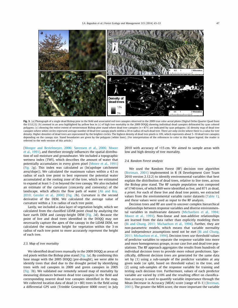
We identified dead trees manually in the 2009 DOQQ as areas ofred pixels within the Bishop pine stand (Fig. 3a). By combining thisbase image with the 2005 DOQQ (pre-drought), we were able toidentify trees that died due to the drought period by identifyingtrees with red canopies in 2009 and green canopies in 2005(Fig. 3b). We validated our remotely sensed map of mortality bymeasuring distances between dead tree canopies in the field andcorresponding nearest dead tree canopies identified in the map.We collected location data of dead (n = 80) trees in the field usinga differential GPS unit (Trimble Geoexplorer 6000 rover) in July

2010 with accuracy of <15 cm. We aimed to sample areas withlow and high density of tree mortality.

2.4. Random Forest analysis

We used the Random Forest (RF) decision tree algorithm(Breiman, 2001) implemented in R (R Development Core Team2010 version 2.12.2) to identify environmental variables that bestexplain the distribution of dead trees, relative to live trees, acrossthe Bishop pine stand. The RF sample population was composedof 1740 trees, of which 869 were identified as live, and 871 as dead,a priori. For each of these live and dead tree points, we extractedvalues from the environmental variable raster datasets (Table 1),and these values were used as input to the RF analysis.

Decision trees and RF are used to uncover complex hierarchicalrelationships between response variables and diverse environmen-tal variables in multivariate datasets (Michaelsen et al., 1994;Moore et al., 1991). Non-linear and non-additive relationshipsare learned from the data rather than explicitly modeling them(Bi and Chung, 2011; Michaelson et al., 1994). Further, they arenon-parametric models, which means that variable normalityand independence assumptions need not be met (Bi and Chung,2011; Michaelson et al., 1994). Decision trees use threshold valuesof predictor variables to separate the response variable into moreand more homogeneous groups, in our case live and dead tree pop-ulations. The RF approach aggregates the results from hundreds ofindividual decision trees to provide more robust predictions. Spe-cifically, different decision trees are generated for the same dataset by (1) using a sub-sample of the predictor variables at anygiven node (or split, based on threshold value) in the tree, and(2) using sub-samples of the response variable for training andtesting each decision tree. Furthermore, values of each predictorvariable are varied by ±10% and the resulting effect on classifica-tion accuracy is used to quantify variable importance through theMean Decrease in Accuracy (MDA) score (range of 0–1) (Breiman,2001). The greater the MDA score, the more important the variable

Fig. 3. (a) Photograph of a single dead Bishop pine in the field and associated red tree canopies observed in the 2009 true color aerial photo (Digital Ortho Quarter Quad fromthe U.S.G.S); (b) zoomed in an area highlighted by yellow box in (c) of high tree mortality in the 2009 DOQQ showing individual dead canopies delineated by cyan coloredpolygons; (c) showing the entire extent of westernmost Bishop pine stand where dead tree canopies (n = 871) are indicated by cyan polygons; (d) density map of dead treecanopies where white circles represent average number of dead tree canopy pixels within a 30 m radius of each dead tree. There are only circles where there is a value for treedensity. Higher densities of dead trees are represented by the brighter circles. The highest density of dead tree pixels is 10%, which represents about 5–10 dead tree canopiesdepending on the canopy size. Stand boundaries are given by the polygons (white lines). (For interpretation of the references to color in this figure legend, the reader isreferred to the web version of this article.)


is in separating live and dead tree populations. While the RF anal-ysis ranks the importance of variables, it does not indicate the nat-ure of the relationships between explanatory variables and thedependent variable. In order to identify and illustrate the natureof these relationships, we compared the histograms of live anddead tree populations for each of these variables, and conducteda Mann–Whitney U test (R version 2.12.2) to test for significant dif-ferences between median values at the p < 0.01 level.

We acknowledge that some of the environmental variables usedin our analysis are interdependent, e.g., slope correlates positivelywith solar insolation and elevation is correlated with cloudiness(Table A2). However, the use of correlated variables in RF analysesbiases neither the classification output (because RF is non-para-metric) nor the measure of variable importance (Peterson et al.,2012; Bi and Chung, 2011).

2.5. Predictive map of tree mortality

We created a predictive map of tree mortality using the RF re-sults and the maps of environmental variables. Specifically, weused the R function ‘yaimpute’ (R version 2.12.2), which takesthe 500 decision trees generated by the RF and applies them tothe environmental variables. The algorithm then averages the500 resulting predictor maps to make one final map. Areas wheretrees are more likely to die following drought are indicated by val-ues closer to one, whereas trees in areas closer to zero are morelikely to live. To better understand what environmental conditionscharacterize areas of low and high mortality during drought, wecompared and contrasted average values of environmental vari-ables at five sites that fall along a coastal inland elevation gradientestablished by Fischer (2007). We examined mortality risk at thesesites for two reasons: (1) sites varied in their levels of probability ofmortality, and (2) field data on fog-water inputs were available forthese locations providing an opportunity for us to relate our remo-tely sensed data of environmental factors with field observationsrelated to potential moisture availability.

3. Results

3.1. Spatial pattern of tree mortality

We were able to accurately identify mortality of nearly 900Bishop pine trees at 1 m spatial resolution (Fig. 3b and c). To moreclearly represent the spatial distribution of dead tree clustersacross the stand, we generated a map of dead tree density(Fig. 3d). While there are many isolated patches of dead trees invarious locations within the stand, we found the highest densityof dead trees to be in the eastern, more inland margin. We assessedthe accuracy of our remote sensing approach with field validationpoints, and found that 30% of the remotely sensed dead trees werewithin 10 m of the ground points (n = 80), and 33% of the deadtrees were between 10 and 20 m (Fig. A2). In addition, visualinspection of the proximity of remotely sensed dead trees tofield-based points revealed good agreement between the twodatasets.

3.2. Relationship between environmental variables and tree mortality

The variables included in our RF analysis formed interacting,hierarchical relationships to distinguish dead (n = 871) from live(n = 869) tree populations within the stand. These variables, how-ever, had different levels of importance (Table 1). Cloud frequencyand elevation received a high rank by the RF analysis (Table 1,MDA: clouds = 0.84, elevation = 0.79), which suggests that the po-sition of trees relative to the summertime stratus cloud layer is

important for reducing the likelihood of mortality. Bishop pineson SCI grow along an elevation gradient that increases from thecoast inland, and along this gradient, summertime cloud cover fre-quency decreases (Fig. A3a). We found most of the dead trees wereclustered at the upper limits of the elevation range within thestand (!360–400 m), where cloud frequency was lowest(Fig. A3b), coinciding with where we observed the greatest treemortality. Live trees spanned a broader range of elevation andcloud frequencies (Fig. A3c). In particular, most Bishop pines thatdied were located at or above 350 m elevation (Fig. 4a, med-ian = 351 m) and where cloud frequency was less than 27%(Fig. 4b, median = 0.26) compared to live trees that were morefrequently found below 300 m (Fig. 4a, median = 279 m) in cloud-ier parts of the stand (Fig. 4b, median = 0.30).

Vegetation height was found to be of roughly equal importanceto cloud cover and elevation in separating live and dead trees(Table 1, MDA: veg. height = 0.81). Dead trees were significantlyshorter than live trees (Fig. 4c; median dead = 7.4 m, medianlive = 9.0 m, p < 0.001). We did not find a correlation between treeheight and any of the environmental factors used in our analysis;however, the spatial distribution of vegetation height indicatesthat taller trees dominate ridges in the southwest portion of thestand where tree mortality was minimal (Fig. 2d).

The remaining topographic variables (solar insolation, slope,and aspect) contributed to distinguishing live and dead treepopulations, yet were ranked lower than cloud frequency, eleva-tion, and vegetation height (Table 1). Nonetheless, the degree ofspread and skewness in the histograms revealed subtle, butinteresting differences between groups. The absolute differencein median solar insolation values between live and dead treepopulations was negligible; however, live trees were normallydistributed over the entire range of solar insolation values,whereas dead trees occurred more often in areas of higher solarinsolation (Fig. 4d; median dead = 19.5 MJ m"2, medianlive = 18.5 MJ m"2, p < 0.001). Additionally, dead trees were foundon more shallow slopes compared to live trees (Fig. 4e; mediandead = 25", median live = 30"). Most Bishop pines (dead or live)grew on northeast-facing slopes, yet live trees were slightly morerestricted to north-facing slopes compared to dead trees (Fig. 4f;median dead = 194 ", live = 203").

Geomorphic variables that characterize the hydrologicenvironment (TWI and curvature) received the lowest MDA rankrelative to other variables in the RF analysis (Table 1). Both liveand dead trees tended to grow in partially channelized areas ofthe landscape as indicated by larger, positive values of TWI(Fig. 4g). The negative curvature values for most of the treesindicate that they also grow in areas with convergent flow lines(Fig. 4h). Certainly Bishop pines grow on ridges as well, but theseresults suggest growing in drainages where more water accumu-lates is important for tree growth, especially during dry years.

Of the three environmental variables with the highest impor-tance (clouds, elevation, and vegetation height), clouds and vegeta-tion height showed linear relationships with probability ofmortality (correlations of 0.54 and 0.48 respectively). Elevationwas not linearly correlated with mortality, though the highimportance value of elevation suggests a non-linear or hierarchicalrelationship.

3.3. Accuracy assessment for Random Forest analysis

An accuracy assessment of the RF analysis allows us to evaluatehow well the RF algorithm classified live and dead trees based onthe reference map we generated from the DOQQ. The accuracy ofRF analysis is evaluated using a confusion matrix from which theProducer’s, User’s, and overall accuracy are derived (Table 2). Pro-ducer’s accuracy refers to the probability that a certain land-cover


category, e.g., dead trees, in the reference map was classified assuch by the RF algorithm (Congalton, 1991). For example, the Pro-ducer’s accuracy of dead trees was 77% because 674 pixels weremodeled as ‘dead’ by the RF algorithm out of the total 871 identi-fied as dead in our reference map. On the other hand, the User’saccuracy refers to the probability that a pixel modeled as ‘dead’is accurately modeled as dead by the RF algorithm (Congalton,1991). For example, the User’s accuracy for dead trees is 78% be-cause 674 pixels were correctly modeled as dead out of the 863 to-tal pixels modeled as such by the RF algorithm. The Producer’s andUser’s accuracy results for live trees were similar to that of deadtrees. Overall, the classification accuracy was high with a score of78% (kappa 0.55). The kappa statistic incorporates misclassificationinformation, so is a more robust measure of accuracy than overallclassification accuracy (Congalton, 1991).

3.4. Predictive map of tree mortality

The predictive map identifies where trees were most vulnerableto drought-induced mortality across the Bishop pine stand giventhe RF results (Fig. 5). We present these results in terms of proba-bility of mortality, where values closer to one indicate a greaterprobability of trees dying through a drought period. We found thatthe probability of mortality in the Bishop pine stand ranged from30% to 75% and that trees growing in eastern and western marginsof the stand were at greater risk of mortality (shades of red/brown)compared to the central and southwest portions of the stand(shades of blue) (Fig. 5).

We compared the probability of mortality and environmentalconditions at five sites that fell along a coastal-to-inland elevationgradient for which we also had fog-water input data collected inthe field (Fischer, 2007) (Table 3). The sites represent the mid-to-high values of the mortality probability scale (54–70%), andfor each area we present the average values of the environmentalpredictor variables (Table 3). Sites were generally characterizedby steep (30–34"), north-facing slopes with moderate solarinsolation (17.6–18.9 MJ m"2). Sites tended to be located in drain-ages (!"0.02–0.13 m m"2) and where water accumulates (TWI,7.9–9.1). There was greater variability in other environmentalpredictive variables across sites.

Site 1 is located at the western margin of the forest stand rela-tively close to the coast. Mortality risk is highest at this site(Table 3; probability of mortality = 70%). Of the five sites, site 1has the highest cloud frequency (32%), yet the lowest average fog

a b c d

e f g h

Fig. 4. Histogram of variables for dead and live tree populations. Differences between median values for live and dead tree populations differed significantly at the p < 0.01level, and values are reported in text. To interpret aspect, north-facing = 180", south-facing = 360", west-facing = 90", and east-facing = 270".

Table 2Average accuracy assessment of 500 decision classification trees in Random Forestanalysis.

Reference

Dead Live Total User’s

Modeled Dead 674 189 863 0.78Live 197 680 877 0.78Total 871 869 1740Producer’s 0.77 0.78Overall accuracy 0.78Kappa 0.55


water input over the summer (597 ml). This is likely attributed toits position below the cloud layer (elevation 141 m). Trees areshorter (5.4 m tall) than at most other sites. Site 2 is slightly higherin elevation (201 m). While less cloudy (28%) than site 1, it receivesmore fog-drip (938 ml) (Table 3). Trees are relatively tall (9.7 m)here and mortality risk low (56%). Site 3 is at higher elevation(423 m), with the highest solar insolation (18.9 MJ m"2) of all thesites. This site has moderate values of cloud cover frequency(26%), fog-drip (1300 ml), vegetation height (7.8 m), and risk ofmortality (63%) relative to other sites. Site 4 is located at the fareastern margin of the Bishop pine stand, close in elevation to site3 (390 m). Probability of mortality (64%) is also similar to that atsite 3. While cloud frequency is low (24%), fog-drip (!1900 ml) ex-ceeded that collected at most other sites. Like site 1, vegetationwas relatively short (6 m). Site 5 is located in the southwest por-tion of the stand at moderate elevation (275 m) where cloud fre-quency is high (31%) and receives the most fog-drip (3205 ml).Trees are tall (11 m) and grow on northwest facing slopes (131").

4. Discussion

4.1. Spatial patterns of tree mortality

We accurately identified approximately 900 dead Bishop pinetree clusters in the largest Bishop pine stand on SCI. While weare confident that the high-spatial resolution of the 2009 DOQQcaptured larger trees with red canopies when the photo wasacquired (Fig. 3b), we believe that we under-sampled smaller trees

(saplings) that we know died during the 2007–2009 drought peri-od, based on field observations. For example, the DOQQ could nothave captured smaller trees growing beneath the canopy of largertrees (Meentemeyer et al., 2008), or simply canopies too small tobe detected at 1-m spatial resolution, e.g., sub-meter diameter orseedlings. Furthermore, we observe that there were smaller treesthat died, or were very close to dead tree canopies, based on thevegetation height data derived from the LiDAR dataset (Fig. 4c),which has much higher precision compared to an aerial photo.

The discrepancy between field-validation points and the remo-tely sensed trees (Fig. A2) was likely attributed to the temporaldisconnect between when we identified dead trees remotely (June2009) and when we collected validation points (July 2010).Because many dead trees that expressed red needles in 2009 hadlost their needles by July 2010, we could not identify in the fieldexactly which trees we identified in our remotely sensed map ofmortality. Despite these shortcomings, the techniques used toidentify dead trees were robust, and feel that we captured themajority of the trees that died in response to drought.

4.2. Environmental controls on tree mortality

Our study demonstrates that there is an inverse relationshipbetween drought-induced mortality of Bishop pines and theoccurrence of summertime clouds along a coastal inland elevationgradient on SCI. The spatial clustering of dead trees in the eastern,and more inland, margin of the stand is consistent with predictionsfrom previous research. Fischer et al. (2009) characterized this area

Fig. 5. Predictive map of tree mortality following drought for our study area (see Fig. 1c for reference). Bishop pine stand is delineated with a black line, and other land surfacetypes are masked out. Red-colored areas represent areas where probability of mortality following drought is high (closer to one) compared to blue-colored areas (closer to 0).Numbered areas (1–5) are described in the text with respect to how probability of mortality relates to environmental conditions and tree height, and are included in Table 3.(For interpretation of the references to colour in this figure legend, the reader is referred to the web version of this article.)

Table 3Average probability of tree mortality and environmental variables for the five sites indicated in Fig. 5. Sample locations were determined based on field sites for which we haddata on fog-water inputs. The area of each site was approximately 20 m2.

Site Probability ofmortality (%)

Avg. summer fog-drip (ml)a

Cloud coverfrequency

Elevation(m)

Vegetationheight (m)

Solar insolation(MJ m"2)

Aspectb

(")Slope(")

Curvature(m m"2)

TWI

1 70 597 0.32 141 5.4 17.8 208 32 0.041 8.12 56 938 0.28 201 9.7 17.6 186 31 "0.033 8.73 63 1300 0.26 423 7.8 18.9 115 30 0.076 9.24 64 1889 0.24 390 6.0 18.0 176 34 0.128 9.15 54 3205 0.31 275 11.1 18.3 131 33 "0.021 7.9

a Fog-drip (ml) data was collected in the field at weather stations (Fischer, 2007) from May–September in 2004. We calculated average volume of fog-water inputs overthese summer months.

b Aspect: north-facing = 180", south-facing = 360", west-facing = 90", and east-facing = 270".


as marginal habitat for Bishop pine based on higher modeled soilwater deficit, which incorporated the cloud frequency variablesused in our analysis, as well as fog water volumes collected fromthe field. The occurrence of fog is spatially heterogeneous, thusthe strength of its impact on reducing water stress and supportingtree growth depends on how it interacts with other landscape andforest elements, such as canopy height.

The vegetation height dataset derived from the 1-m LiDAR DEMprovided us with a unique opportunity to address how character-istics of vegetation interact with climatic and landscape variables.We found that larger trees (>8 m tall) that occurred in cloudier, andthus foggier, areas (!30% summertime cloud frequency, Figs. 2aand 3d) had high survivorship following drought. This agrees withprevious research that showed Bishop pines had higher summer-time growth rates in the cloudier portion of the stand comparedto trees that grow further inland and at higher elevation (Carboneet al., 2012). The positive relationship between fog frequency, treesize, and survivability could be explained by the fact that largertrees having a greater capacity to intercept fog and generate fogdrip to the soil, which can significantly offset the effects of droughtstress and support growth even during low rainfall years (Carboneet al., 2012; Fischer et al., 2009). Therefore, fogginess may confer afitness advantage over trees that grow in the less foggy, and morexeric parts of the stand (del-Val et al., 2006), which has importantimplications for the local distribution of trees that persist at thewater-limited extent of the species range.

4.3. Environmental heterogeneity and probability of mortality

The occurrence of low-stratus clouds in the summertime is notthe only factor important to the survival of Bishop pine trees dur-ing drought. Complex and subtle interactions between climate,topography, and vegetation can have large effects on plant-avail-able water, and the suitability of habitat for growth and survival.We observed that the three main distinguishing factors betweensites with the highest and lowest mortality risk (Table 3; site 1and site 5, respectively) were elevation, volume of fog-drip, andvegetation height (Table 3). Because cloudiness was equally highat both sites (!31–32%), the large difference in fog water input isattributed to where the low-stratus clouds are intercepted by land.Based on a climatology of cloud base heights from the Santa Bar-bara airport, interception of low-stratus clouds is 40% more likelyat sites between 240 and 280 m than at lower elevation (B. Rastogi,pers. comm). Therefore, topographic relief is necessary for cloudi-ness to translate to direct fog water inputs, which influencesplant-available water (Fischer, 2007). In addition, trees were twiceas tall at site 5 than site 1 (Table 3).

The probability of mortality was similarly low between sites 2and 5. While these sites supported the tallest trees, they were dis-similar with respect to other environmental variables. Unlike site5, site 2 is located at the mouth of a large drainage in the centralvalley on SCI, which supports cool, wet conditions compared tosites located in more exposed areas. Because ridges rise steeplyfrom the valley floor, this site is also located on a steep, north-fac-ing slope, which explains why solar insolation was low comparedto other sites (Table 3).

The similarity in probability of mortality at sites 3 and 4 (63%and 64%, respectively) coincide with many of the environmentalfactors that characterize these sites. Located on ridges at the upperlimit of the elevation range for Bishop pines on the island (!400 m)where cloud frequency was relatively low (24–26%) suggests thatthe evaporative losses may dominate at these sites. The distin-guishing factor between these sites, other than measured fog-drip,is vegetation height. Trees are taller at site 3, therefore may havegreater access to groundwater, which could compensate for lowerfog-water inputs. Conversely, trees at site 4 are shorter, but grow

on steeper slopes and are less exposed, thus buffered from dryingeffects.

The results of our study indicate that microhabitat conditions inthe Bishop pine stand on SCI are critical for determining thesurvival and persistence of trees during exceptionally warm, dryperiods. However, just as environmental conditions can varywidely across a forested ecosystem, many studies have demon-strated that variation in physiological adjustments of trees tostressful conditions, and differential growth patterns, are strongpredictors of spatial patterns of mortality in forests (McDowellet al., 2008; Suarez et al., 2004; Wycoff and Clark, 2002; Ogleet al., 2000; Pederson, 1998; Cregg, 1994). While we did notexplicitly test for variation in physiological responses or growthof Bishop pine trees in response to drought, we did find mortalityrisk varied among trees of different size classes. The probability ofmortality was greater for shorter trees, even if the height differencewas only 1–2 m (Fig. 4d). One possible explanation for this patterncould be that smaller trees have limited access to stable waterreserves deeper in the soil, thus are at a disadvantage duringdrought periods compared to larger trees that have a greaterroot:shoot ratio (Suarez et al., 2004). Another interpretation of thispattern may be related to how drought has historically affectedpopulation dynamics (i.e., tree age and size structure) in the Bishoppine stand.

The most recent drought period (2007–09) was not an isolatedevent. Periodic droughts have affected the local distribution ofBishop pine on SCI in the past (Walter and Taha, 2000). The lastmajor drought occurred between years 1986 and 1991, and killedoff large swaths of Bishop pines across the island, particularly atthe margins of the Bishop pine stands (Walter and Taha, 2000;Lyndal Laughrin, pers. comm.). Our results support the idea thatsurvivorship of Bishop pine trees is compromised at the stand mar-gins during drought (Fig. 3). However, regeneration of the pinepopulation in these areas has not ceased (Fischer et al., 2009).The net effect of these drought cycles are even-aged cohorts dom-inating the stand margins. Therefore, the majority of trees weobserved die after the most recent drought likely emerged follow-ing the previous drought that ended in 1991; thus, they wereyounger and had a shorter stature than the trees more resilientto drought stress that dominate the central and southwest partsof the stand.

4.4. Implications for management

Analyzing high-spatial resolution (1 m) aerial imagery andLiDAR remotely sensed data of tree mortality can provide moreprecise spatial information about the growing conditions ofindividual trees, or small tree clusters, and provide a more efficientapproach to forest inventory (Hicke et al., 2012; Maggi andMeentemeyer, 2002). Specifically, the color infrared DOQQ usedin our study clearly showed red-attack trees allowing us todelineate dead tree canopies. DOQQ imagery is available at no costand collected 2–3 times per decade for any given local in theUnited States; therefore, acquiring and analyzing imagery thatbookends a mortality event is feasible, allowing for a cost-effectivemethod of inventorying forest damage. In contrast, LiDAR data isexpensive and not readily available but the utility of derivingvegetation height and landscape variables was clearly demon-strated in this project.

We found RF to be a power statistical tool for analyzing a largemultivariate dataset that ranked a suite of environmental variablesused to predict tree mortality. This approach can be used in a vari-ety of forest management applications that require analysis oflarge datasets where there may be correlation among the predic-tors and hierarchical and/or non-linear relationships betweenpredictor and response variables.


This study supports the idea that low-stratus summertimeclouds are important to survival of Bishop pines during droughtperiods at the most southern and water-limited extent of its range.However, the distribution of this species is restricted to the narrowfog-belt of California, despite the fact that precipitation is muchhigher further north, so fog must play a role in the more northernparts of the range as well. There is a great amount of uncertaintysurrounding how the spatial and temporal variability of fog maychange in the future; however, evidence suggests that fog fre-quency may decline in parts of the California coastline (Johnstoneand Dawson, 2010), which would have negative effects on the dis-tribution of Bishop pines and other fog-dependent species.

Acknowledgements

This work was funded by a grant from the Kearney Foundationof Soil Science. We would like to thank Carla D’Antonio, JenniferKing, and Doug Fischer for helpful comments and valuablesuggestions; Ryan Perroy for assistance in the field. We thank theNature Conservancy and the University of California NaturalReserve System for access to southwestern Santa Cruz Island.

Appendix A. Supplementary material

Supplementary data associated with this article can be found, inthe online version, at http://dx.doi.org/10.1016/j.foreco.2013.12.020.

References

Adams, H.D., Guardiola-Claramonte, M., Barron-Gafford, G.A., Villegas, J.C.,Breshears, D.D., Zou, C.B., Troch, P.A., Huxman, T.E., 2009. Temperaturesensitivity of drought-induced tree mortality portends increased regional die-off under global-change-type drought. Proc. Natl. Acad. Sci. 106, 7063–7066.

Ali, G.A., Roy, A.G., 2010. Shopping for hydrologically representative connectivitymetrics in a humid temperate forested catchment. Water Resour. Res. 46,W12544.

Allen, C.D., Breshears, D.D., 1998. Drought-induced shift of a forest-woodlandecotone: rapid landscape response to climate variation. Proc. Natl. Acad. Sci. 95,14839–14842.

Allen, C.D., Macalady, A.K., Chenchouni, H., Bachelet, D., McDowell, N., Vennetier,M., Kitzberger, T., Rigling, A., Breshears, D.D., Hogg, E.H. (Ted)., Gonzalez, P.,Fensham, R., Zhang, Z., Castro, J., Demidova, N., Lim, J.H., Allard, G., Running,S.W., Semerei, A., Cobb, N., 2010. A global overview of drought and heat-induced tree mortality reveals emerging climate change risks for forests. ForestEcol. Manage. 259, 660–684.

Anderegg, W.R.L., Berry, J.A., Smith, D.D., Sperry, J.S., Anderegg, L.D.L., Field, C.B.,2012. The roles of hydraulic and carbon stress in a widespread climate-inducedforest die-off. Proc. Natl. Acad. Sci. 109, 233–237.

Anderson, L.O., Malhi, Y., Aragão, L.E., Ladle, R., Arai, E., Barbier, N., Phillips, O., 2010.Remote sensing detection of droughts in Amazonian forest canopies. NewPhytologist 187, 733–750.

Azevedo, J., Morgan, D.L., 1974. Fog precipitation in coastal California forests.Ecology, 1135–1141.

Barbosa, O., Marquet, P.A., Bacigalupe, L.D., Christie, D.A., Del-Val, E., Gutierrez, A.G.,Jones, C.G., Weathers, K.C., Armesto, J.J., 2010. Interactions among patch area,forest structure and water fluxes in a fog-inundated forest ecosystem in semi-arid Chile. Funct. Ecol. 24, 909–917.

Bi, J., Chung, J., 2011. Identification of drivers of overall liking-determination ofrelative importances of regressor variables. J. Sens. Stud. 26, 245–254.

Breiman, L., 2001. Random forests. Machine Learning 45, 5–32.Breshears, D.D., Cobb, N.S., Rich, P.M., Price, K.P., Allen, C.D., Balice, R.G., Romme,

W.H., Kastens, J.H., Floyd, M.L., Belnap, J., Anderson, J.J., Myers, O.B., Meyer, C.W.,2005. Regional vegetation die-off in response to global-change-type drought.Proc. Natl. Acad. Sci. 102, 15144–15148.

Carbone, M.S., Williams, A.P., Ambrose, A.R., Boot, C.M., Bradley, E.S., Dawson, T.E.,Schaeffer, S.M., Schimel, J.P., Still, C.J., 2012. Cloud shading and fog dripinfluence the metabolism of a coastal pine ecosystem. Global Change Biol. 19,484–497.

Cavender-Bares, J., Bazzaz, F.A., 2000. Changes in drought response strategies withontogeny in Quercus rubra: implications for scaling from seedings to maturetrees. Oecologia 124, 8–18.

Cavelier, J., Solis, D., Jaramillo, M.A., 1996. Fog interception in montane forestsacross the Central Cordillera of Panama. J. Tropical Ecol. 12, 357–369.

Chambers, J.Q., Asner, G.P., Morton, D.C., Anderson, L.O., Saatchi, S.S., Espírito-Santo,F.D.B., Palace, M., Souza, C., 2007. Regional ecosystem structure and function:

ecological insights from remote sensing of tropical forests. Trends Ecol. Evol. 22,414–423.

Clark, D.B., Castro, C.S., Alvarado, L.D.A., Read, J.M., 2004. Quantifying mortality oftropical rain forest trees using high-spatial-resolution satellite data. Ecol. Lett.,52–59.

Congalton, R.G., 1991. A review of assessing the accuracy of classifications ofremotely sensed data. Remote Sens. Environ. 46, 35–46.

Coops, N.C., Johnson, M., Wulder, M.A., White, J.C., 2006. Assessment of QuickBirdhigh spatial resolution imagery to detect red attack damage due to mountainpine beetle infestation. Remote Sens. Environ. 103, 67–80.

Corbin, J.D., Thomsen, M.A., Dawson, T.E., D’Antonio, C.M., 2005. Summer water useby California coastal prairie grasses: fog, drought, and community composition.Oecologia 145, 511–521.

Cregg, B.M., 1994. Carbon allocation, gas exchange, and needle morphology of Pinusponderosa genotypes known to differ in growth and survival under imposeddrought. Tree Physiol. 14, 883–898.

Dawson, T.E., 1996. Determining water use by trees and forests from isotopic,energy balance and transpiration analyses: the roles of tree size and hydrauliclift. Tree Physiol. 16, 263–272.

Dawson, T.E., 1998. Fog in the California redwood forest: ecosystem inputs and useby plants. Oecologia 117, 476–485.

Dennison, P.E., Brunelle, A.R., Carter, V.A., 2010. Assessing canopy mortality during amountain pine beetle outbreak using GeoEye-1 high spatial resolution satellitedata. Remote Sens. Environ. 114, 2431–2435.

del-Val, E., Armesto, J.J., Barbosa, O., Christie, D.A., Gutiérrez, A.G., Jones, C.G.,Marquet, P.A., Weathers, K.C., 2006. Rain forest islands in the Chilean semiaridregion: fog-dependency, ecosystem persistence and tree regeneration.Ecosystems 9, 598–608.

Donovan, L.A., Ehleringer, J.R., 1994. Water stress and use of summer precipitationin a Great Basin shrub community. Funct. Ecol. 8, 289–297.

Dubayah, R.C., 1994. Modeling a solar radiation topoclimatology for the rio granderiver basin. J. Vegetation Sci. 5, 627–640.

Edburg, S.L., Hicke, J.A., Brooks, P.D., Pendall, E.G., Ewers, B.E., Norton, U., Gochis, D.,Gutmann, E.D., Meddens, A.J., 2012. Cascading impacts of bark beetle-causedtree mortality on coupled biogeophysical and biogeochemical processes. Front.Ecol. Environ. 10, 416–424.

Ewing, H.A., Weathers, K.C., Templer, P.H., Dawson, T.E., Firestone, M.K., Elliott, A.M.,Boukili, V.K., 2009. Fog water and ecosystem function: heterogeneity in aCalifornia redwood forest. Ecosystems 12, 417–433.

Fischer, D.T., 2007. Ecological and Biogeographic Impacts of Fog and Stratus Cloudson Coastal Vegetation, Santa Cruz Island, CA (Doctoral Disserations). Universityof California, Santa Barbara, CA.

Fischer, D.T., Still, C.J., Williams, A.P., 2009. Significance of summer fog and overcastfor drought stress and ecological functioning of coastal California endemic plantspecies. J. Biogeography 36, 783–799.

Floyd, M.L., Clifford, M., Cobb, N.S., Hanna, D., Delph, R., Ford, P., Turner, D., 2009.Relationship of stand characteristics to drought-induced mortality in threeSouthwestern pinon-juniper woodlands. Ecol. Appl. 19, 1223–1230.

Fraser, R.H., Latifovic, R., 2005. Mapping insect-induced tree defoliation andmortality using coarse spatial resolution satellite imagery. Int. J. Remote Sens.26, 193–200.

Gessler, P.E., Chadwick, O.A., Chamran, F., Althouse, L., Holmes, K., 2000. Modelingsoil – landscape and ecosystem properties using terrain attributes. Soil Sci. Soc.Am. 64, 2046–2056.

Gitlin, A.R., Sthultz, C.M., Bowker, M.A., Stumpf, S., Paxton, K.L., Kennedy, K., Muñoz,A., Bailey, J.K., Whitham, T.G., 2006. Mortality gradients within and amongdominant plant populations as barometers of ecosystem change during extremedrought. Conservation Biol. 20, 1477–1486.

Guo, Q., Kelly, M., Gong, P., Liu, D., 2007. An object-based classification approach inmapping tree mortality using high spatial resolution imagery. GIScienceRemote Sens. 44, 24–47.

Gutierrez, A.G., Barbosa, O., Christie, D.A., del-Val, E.K., Ewing, H.A., Jones, C.G.,Marquet, P.A., Weathers, K.C., Armesto, J.J., 2008. Regeneration patterns andpersistence of the fog-dependent Fray Jorge forest in semiarid Chile during thepast two centuries. Global Change Biol. 14, 161–176.

Hanson, P.J., Weltzin, J.F., 2000. Drought disturbance from climate change: responseof United States forests. Sci. Total Environ. 262, 205–220.

Harr, R.D., 1982. Fog drip in the Bull Run municipal watershed, Oregon. WaterResour. Bull. 18, 785–789.

Hetrick, W.A., Rich, M.P., Barnes, F.J., Weiss, S.B., 1993. GIS-based solar radiation fluxmodels. Am. Soc. Photogrammetry Remote Sens. Tech. Pap. 3, 132–143.

Hicke, J.A., Johnson, M.C., Hayes, J.L., Preisler, H.K., 2012. Effects of bark beetle-caused tree mortality on wildfire. Forest Ecol. Manage. 271, 81–90.

Hicke, J.A., Logan, J., 2009. Mapping whitebark pine mortality caused by a mountainpine beetle outbreak with high spatial resolution satellite imagery. Int. J.Remote Sens. 30, 4427–4441.

Huang, C.-Y., Anderegg, W.R.L., 2012. Large drought-induced aboveground livebiomass losses in southern Rocky Mountain aspen forests. Global Change Biol.18, 1016–1027.

Hutley, L.B., Doley, D., Yates, D.J., Boonsaner, A., 1997. Water balance of anAustralian subtropical rainforest at altitude: the ecological and physiologicalsignificance of intercepted cloud and fog. Aust. J. Bot. 45, 311–329.

Ingraham, N., Matthews, R., 1995. The importance of fog-drip water to vegetation:Point Reyes Peninsula, California. J. Hydrol. 164, 269–285.

Iacobellis, S.F., Cayan, D.R., 2013. The variability of California summertime marinestratus: Impacts on surface air temperatures. J. Geophys. Res.: Atmos. 118, 1–18.


Johnstone, J.A., Dawson, T.E., 2010. Climatic context and ecological implications ofsummer fog decline in the coast redwood region. Proc. Natl. Acad. Sci. 107,4533–4538.

Junak, S., Ayers, T., Scott, R., Wilken, D., Young, D.A., 1995. A flora of Santa CruzIsland. Santa Barbara Botanical Garden, Santa Barbara, California.

Koepke, D.F., Kolb, T.E., Adams, H.D., 2010. Variation in woody plant mortality anddieback from severe drought among soils, plant groups, and species within anorthern Arizona ecotone. Oecologia 163, 1079–1090.

Lanner, R.L., 1999. Conifers of California. Cachuma Press, Los Olivos, CA.Limm, E.B., Simonin, K.A., Bothman, A.G., Dawson, T.E., 2009. Foliar water uptake: a

common water acquisition strategy for plants of the redwood forest. Oecologia161 (3), 449–459.

Limm, E.B., Dawson, T.E., 2010. Polystichum munitum (Dryopteridaceae) variesgeographically in its capacity to absorb fog water by foliar uptake within theredwood forest ecosystem. Am. J. Bot. 97 (7), 1121–1128.

McDowell, N., Pockman, W.T., Allen, C.D., Breshears, D.D., Cobb, N., Kolb, T., Plaut, J.,Sperry, J., West, A., Williams, D.G., Yepez, E.A., 2008. Mechanisms of plantsurvival and mortality during drought: why do some plants survive whileothers succumb to drought? New Phytologist 178, 719–733.

Macomber, S.A., Woodcock, C.E., 1994. Mapping and monitoring conifer mortalityusing remote sensing in the lake tahoe basin. Remote Sens. Environ. 266, 255–266.

Maggi, K., Meentemeyer, R.K., 2002. Landscape dynamics of the spread of suddenoak death. Photogrammetric Eng. Remote Sens. 68, 1001–1009.

Meigs, G.W., Kennedy, R.E., Cohen, W.B., 2011. A Landsat time series approach tocharacterize bark beetle and defoliator impacts on tree mortality and surfacefuels in conifer forests. Remote Sens. Environ. 115, 3707–3718.

Meentemeyer, R.K., Rank, N.E., Shoemaker, D.A., Oneal, C.B., Wickland, A.C.,Frangioso, K.M., Rizzo, D.M., 2008. Impact of sudden oak death on treemortality in the Big Sur ecoregion of California. Biol. Invasions 10, 1243–1255.

Michaelsen, J., Schimel, D.S., Friedl, M.A., Davis, F.W., Dubayah, Ralph C., 1994.Regression tree analysis of satellite and terrain data to guide vegetationsampling and surveys. J. Vegetation Sci. 5, 673–686.

Monger, H., Bestelmeyer, B., 2006. The soil-geomorphic template and biotic changein arid and semi-arid ecosystems. J. Arid Environ. 65, 207–218.

Moore, D.M., Lees, B.G., Davey, S.M., 1991. A new method for predicting vegetationdistributions using decision tree analysis in a geographic information system.Environ. Manage. 15, 59–71.

Ogle, K., Whitham, T.G., Cobb, N.S., 2000. Tree-ring variation in pinyon predictslikelihood of death following severe drought. Ecology 81, 3237–3243.

Pederson, B.S., 1998. The role of stress in the mortality of Midwestern oaks asindicated by growth prior to death. Ecology 79, 79–93.

Perroy, R.L., Bookhagen, B., Asner, G.A., Chadwick, O.A., 2010. Comparison of gullyerosion estimates using airborne and ground-based LiDAR on Santa Cruz Island,California. Geomorphology 118, 288–300.

Perroy, R.L., Bookhagen, B., Chadwick, O.A., Howarth, J.T., 2012. Holocene andanthropocene landscape change: arroyo formation on Santa Cruz Island,California. Ann. Assoc. Am. Geographers 102, 1229–1250.

Peterson, S.H., Franklin, J., Roberts, D.A., van Wagtendonk, J.W., 2012. Mapping fuelsin Yosemite National Park. Can. J. Forest Res. 43, 7–17.

Ponette-Gonzalez, A.G., Weathers, K.C., Curran, L.M., 2010. Water inputs across atropical montane landscape in Veracruz, Mexico: synergistic effects of landcover, rain and fog seasonality, and interannual precipitation variability. GlobalChange Biol. 16, 946–963.

Raven, P.H., Axelrod, D.I., 1978. Origin and Relationships of the California Flora.University of California Press, Berkeley, CA.

Sørensen, R., Zinko, U., Seibert, J., 2006. On the calculation of the topographicwetness index: evaluation of different methods based on field observations.Hydrol. Earth Syst. Sci. 10, 101–112.

Stone, C., Penman, T., Turner, R., 2012. Managing drought-induced mortality in Pinusradiata plantations under climate change conditions: a local approach usingdigital camera data. Forest Ecol. Manage. 265, 94–101.

Suarez, M.L., Ghermandi, L., Kitzberger, T., 2004. Factors predisposing episodicdrought-induced mortality in Nothofagus-site, climatic sensitivity and growthtrends. J. Ecol. 92, 954–966.

Uehara, Y., Kume, A., 2012. Canopy rainfall interception and fog capture by pinuspumila regal at Mt. Tateyama in the Northern Japan Alps, Japan. Arctic,Antarctic, Alpine Res. 44, 143–150.

van Mantgem, P.J., Stephenson, N.L., Byrne, J.C., Daniels, L.D., Franklin, J.F., Fulé, P.Z.,Harmon, M.E., Larson, A.J., Smith, J.M., Taylor, A.H., Veblen, T.T., 2009.Widespread increase of tree mortality rates in the western United States.Science 323, 521–524.

Vogelmann, H.W., 1973. Fog precipitation in the cloud forests of eastern Mexico.Bioscience 23 (2), 96–100.

Walter, H.S., Taha, L.A. 2000. Regeneration of Bishop pine (Pinus muricata) in theabsence and presence of fire: a case study from Santa Cruz Island, California. In:Browne, D.R., Mitchell, K.L., Chaney, H.W. (Eds.), Proceedings of the fifthCalifornia Islands symposium, 1999 March 29 to April 1, Santa Barbara,California. San Diego, CA, U.S. Department of the Interior, Mineral ManagementService (OCS Study MMS 99–0038), pp. 172–181.

Weathers, K.C., Lovett, G.M., Likens, G.E., 1995. Cloud deposition to a spruce forestedge. Atmos. Environ. 29, 665–672.

Williams, A.P., Still, C.J., Fischer, D.T., Leavitt, S.W., 2008. The influence ofsummertime fog and overcast clouds on the growth of a coastal Californianpine: a tree-ring study. Oecologia 156, 601–611.

Williams, A.P., 2009. Teasing foggy memories out of Pines on the California ChannelIslands using Tree-Ring width and Stable Isotope approaches (Doctoraldisserations). University of California, Santa Barbara, CA.

Williams, A.P., Allen, C.D., Millar, C.I., Swetnam, T.W., Michaelsen, J., Still, C.J.,Leavitt, S.W., 2010. Forest responses to increasing aridity and warmth in thesouthwestern United States. Proc. Natl. Acad. Sci. 107, 21289–21294.

Wulder, M.A., Dymond, C.C., White, J.C., Leckie, D.G., Carroll, A.L., 2006. Surveyingmountain pine beetle damage of forests: a review of remote sensingopportunities. Forest Ecol. Manage. 221, 27–41.

Wycoff, P.H., Clark, J.S., 2002. The relationship between growth and mortality forseven co-occurring tree species in the southern Appalachian Mountains. J. Ecol.90, 604–615.


Forest Ecology and Management - University of …bodo/pdf/baguskas14_SCI_tree...Evaluating spatial...

Documents

Transcript of Forest Ecology and Management - University of …bodo/pdf/baguskas14_SCI_tree...Evaluating spatial...