Foreign Currency Bank Funding and Global Factors

Signe Krogstrup

International Monetary Fund

skrogstrup@imf.org

and

Cedric Tille

The Graduate Institute of International and Development Studies

cedric.tille@graduateinstitute.ch

September 1, 2017

Abstract

The literature on the drivers of international capital flows establishes the importance of

global financial risk factors. However, the cross country and time variation in the sensi-

tivity of capital flows to global factors is substantial and not well understood. We present

a portfolio balance model suggesting that the foreign currency mismatch on financial in-

stitutions’ balance sheets determine the size and sign of these institutions’ cross border

flows in response to global risk factors. Testing the model for European banks’ net foreign

currency funding flows yields supporting evidence, especially for countries that are not

members of the euro area.

JEL Classification: F32, F34, F36.

Keywords: Currency mismatch, push factors, spillovers, cross-border transmission of shocks,

European bank balance sheets.

The views in this paper are solely the responsibility of the authors and do not necessarily reflect the viewsof the International Monetary Fund, its Executive Board or Management. We would like to thank GiovanniDell’Ariccia, Oliver Gloede, Linda Goldberg, Alistair Milne, Philip Saure, Casper de Vries, Adrian van Rix-tel, Pinar Yesin, participants at the SNB workshop on foreign currency lending, the Infinity conference, theKonstanz seminar, the annual meeting of the Swiss Society of Economics and Statistics, an SNB brownbagworkshop, the BIS SNB research workshop, an IMF Research Seminar and a Federal Reserve Board brownbagseminar, for comments and suggestions on the present and earlier versions of this paper. Excellent researchassistance was provided by Menglu Cai.

1 Introduction

How do capital flows respond to global risk factors? It is well established in the empirical

literature that conditions in global financial markets, such as global risk sentiment, volatility

and liquidity, drive cross border capital flows (e.g. Calvo et al. [1996], Forbes and Warnock

[2012a], Rey [2015], Cerutti et al. [2016]). Global financial factors have traditionally been

viewed as push factors in the literature, impacting capital flows irrespective of the fundamen-

tals of recipient countries. Accordingly, they are usually modelled as having a uniform impact

on capital flows over time and across countries. Recent empirical studies point to substan-

tial cross country variation in the response of cross border capital flows to global financial

factors, however, and to changes in the sensitivity of capital flows to global factors over time

(e.g. Avdjiev et al. [2016c], Cerutti et al. [2017]). These patterns are not just a reflection

of differences between emerging markets and advanced economies, as time and cross country

variation is also manifested within these sets of countries (Goldberg and Krogstrup [2016]).

It underscores that country specific features play a role in determining a country’s capital

flow sensitivity to global factors and, hence, capital flow volatility.

An understanding of how country specific features drive capital flow sensitivity to global

factors can help inform the design of capital flow management measures. The literature

on the drivers of capital flow sensitivity to global factors is scarce, however. Two recent

empirical studies suggest that the types of foreign investors and domestic financial institutions

intermediating a country’s cross border capital flows play a role (IMF [2014], Cerutti et al.

[2015])), although the exact mechanisms remain unexplored. Cross country comparable data

on the financial market structure underlying cross border flows are limited, and there is, to

our knowledge, no theoretical literature investigating the determinants of a country’s capital

flow sensitivity to global risk factors.

This paper contributes to the theoretical as well as the empirical understanding of the

drivers of a country’s capital flow sensitivity to global factors. Building on the role of financial

institutional structure underlined in IMF [2014] and Cerutti et al. [2015], we focus on the

role of the balance sheet structure of a country’s financial institutions and illustrate that

their foreign currency mismatch can affect the sign and size of the response of capital flows

to global risk factors. The mechanism is the following. Financial institutions choose their

foreign currency exposure to maximize a risk-adjusted return on their total portfolio. When

the risk associated with their foreign currency exposure increases, a country’s resident financial

institutions will respond by reducing their foreign currency exposure, given expected returns.

Reducing foreign currency exposure, however, has different implications for the direction

of the resulting cross border flow depending on the sign of financial institutions’ foreign

1

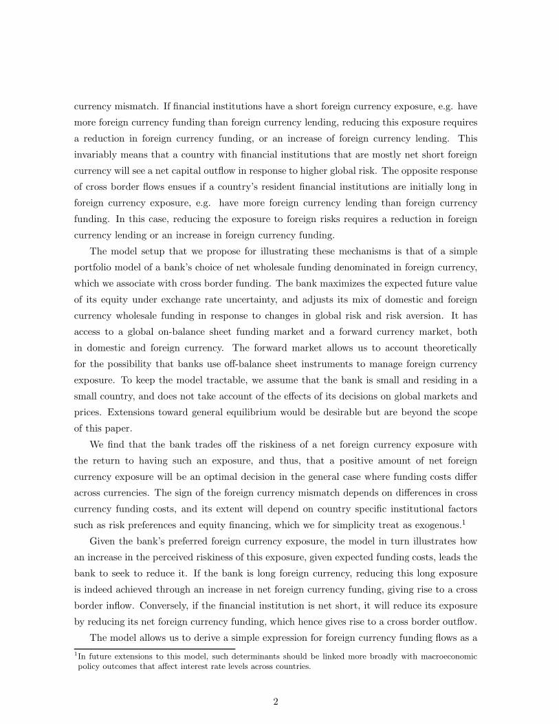
currency mismatch. If financial institutions have a short foreign currency exposure, e.g. have

more foreign currency funding than foreign currency lending, reducing this exposure requires

a reduction in foreign currency funding, or an increase of foreign currency lending. This

invariably means that a country with financial institutions that are mostly net short foreign

currency will see a net capital outflow in response to higher global risk. The opposite response

of cross border flows ensues if a country’s resident financial institutions are initially long in

foreign currency exposure, e.g. have more foreign currency lending than foreign currency

funding. In this case, reducing the exposure to foreign risks requires a reduction in foreign

currency lending or an increase in foreign currency funding.

The model setup that we propose for illustrating these mechanisms is that of a simple

portfolio model of a bank’s choice of net wholesale funding denominated in foreign currency,

which we associate with cross border funding. The bank maximizes the expected future value

of its equity under exchange rate uncertainty, and adjusts its mix of domestic and foreign

currency wholesale funding in response to changes in global risk and risk aversion. It has

access to a global on-balance sheet funding market and a forward currency market, both

in domestic and foreign currency. The forward market allows us to account theoretically

for the possibility that banks use off-balance sheet instruments to manage foreign currency

exposure. To keep the model tractable, we assume that the bank is small and residing in a

small country, and does not take account of the effects of its decisions on global markets and

prices. Extensions toward general equilibrium would be desirable but are beyond the scope

of this paper.

We find that the bank trades off the riskiness of a net foreign currency exposure with

the return to having such an exposure, and thus, that a positive amount of net foreign

currency exposure will be an optimal decision in the general case where funding costs differ

across currencies. The sign of the foreign currency mismatch depends on differences in cross

currency funding costs, and its extent will depend on country specific institutional factors

such as risk preferences and equity financing, which we for simplicity treat as exogenous.1

Given the bank’s preferred foreign currency exposure, the model in turn illustrates how

an increase in the perceived riskiness of this exposure, given expected funding costs, leads the

bank to seek to reduce it. If the bank is long foreign currency, reducing this long exposure

is indeed achieved through an increase in net foreign currency funding, giving rise to a cross

border inflow. Conversely, if the financial institution is net short, it will reduce its exposure

by reducing its net foreign currency funding, which hence gives rise to a cross border outflow.

The model allows us to derive a simple expression for foreign currency funding flows as a

1In future extensions to this model, such determinants should be linked more broadly with macroeconomicpolicy outcomes that affect interest rate levels across countries.

2

function of changes in global risk factors, pre-existing currency exposures, and other determi-

nants of the risk and return of funding positions, from which we derive an empirical estimating

equation. This estimating equation is then taken to the data for cross border bank funding

flows in foreign currency. Even though the model predictions extend more generally to flows

associated with other types of institutions, we focus on bank flows because the richness of

cross-country comparable bank balance sheet data allows us to compute specific types of flows

and associate these directly with features of the balance sheets of the institutions intermediat-

ing the flows. Specifically, we use a novel data set for European countries’ aggregate banking

sector balance sheets. This data set is compiled by the Swiss National Bank in collabora-

tion with central banks of participating European countries. It distinguishes between banks’

domestic and foreign counterparties as well as positions in local and foreign currency, the

latter being further divided into Swiss francs and other foreign currencies. We obtain cross

border foreign currency flows by valuation adjusting the quarterly changes in outstanding po-

sitions using additional country specific data sources on the currency breakdown of positions

in non-Swiss franc foreign currencies.

A remaining data challenge is the lack of information on off-balance sheet foreign currency

exposures, which can be an important part of banks’ total foreign currency exposures. We

instead use on-balance sheet foreign currency exposure as a proxy, and control empirically for

drivers of the use of off-balance sheet foreign currency instruments by including deviations

from covered interest parity, as suggested by the model. This source of imprecision could

attenuate our results. The results, however, confirm the main predictions of the model. The

global risk factor is not significant on its own, but becomes significant when interacted with

foreign currency exposure. We find that the effect is most pronounced, and very robust,

in countries outside the euro area, while global factors do not significantly explain foreign

currency funding flows in countries that use the euro. This difference could be related to

differences in foreign currency hedging practises across the two country samples. We also

find that the most consistently empirically relevant measure of the global financial factor

is growth in US broker dealer leverage, as proposed notably in Adrian and Shin [2014].

Alternative measures often used in the literature, such as the V IX and measures of US

financial conditions, are not significant in the sample that we consider.

Our model and empirical findings underline that global factors are not just indiscriminate

push factors, and that both the size and sign of a country’s capital flow sensitivity to global

factors depends on institutional features associated with the set of financial institutions in-

volved in intermediating a country’s cross border flows. Specifically, our findings imply that

currency mismatches in the balance sheets of a country’s financial institutions may not only

increase a country’s vulnerability to capital flow volatility, but could directly influence the

3

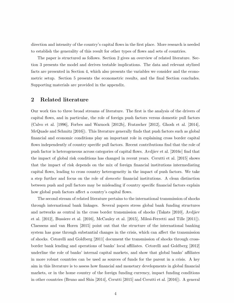
direction and intensity of the country’s capital flows in the first place. More research is needed

to establish the generality of this result for other types of flows and sets of countries.

The paper is structured as follows. Section 2 gives an overview of related literature. Sec-

tion 3 presents the model and derives testable implications. The data and relevant stylized

facts are presented in Section 4, which also presents the variables we consider and the econo-

metric setup. Section 5 presents the econometric results, and the final Section concludes.

Supporting materials are provided in the appendix.

2 Related literature

Our work ties to three broad streams of literature. The first is the analysis of the drivers of

capital flows, and in particular, the role of foreign push factors versus domestic pull factors

(Calvo et al. [1996], Forbes and Warnock [2012b], Fratzscher [2012], Ghosh et al. [2014],

McQuade and Schmitz [2016]). This literature generally finds that push factors such as global

financial and economic conditions play an important role in explaining cross border capital

flows independently of country specific pull factors. Recent contributions find that the role of

push factor is heterogeneous across categories of capital flows. Avdjiev et al. [2016c] find that

the impact of global risk conditions has changed in recent years. Cerutti et al. [2015] shows

that the impact of risk depends on the mix of foreign financial institutions intermediating

capital flows, leading to cross country heterogeneity in the impact of push factors. We take

a step further and focus on the role of domestic financial institutions. A clean distinction

between push and pull factors may be misleading if country specific financial factors explain

how global push factors affect a country’s capital flows.

The second stream of related literature pertains to the international transmission of shocks

through international bank linkages. Several papers stress global bank funding structures

and networks as central in the cross border transmission of shocks (Takats [2010], Avdjiev

et al. [2012], Bussiere et al. [2016], McCauley et al. [2015], Milesi-Ferretti and Tille [2011]).

Claessens and van Horen [2015] point out that the structure of the international banking

system has gone through substantial changes in the crisis, which can affect the transmission

of shocks. Cetorelli and Goldberg [2011] document the transmission of shocks through cross-

border bank lending and operations of banks’ local affiliates. Cetorelli and Goldberg [2012]

underline the role of banks’ internal capital markets, and show that global banks’ affiliates

in more robust countries can be used as sources of funds for the parent in a crisis. A key

aim in this literature is to assess how financial and monetary developments in global financial

markets, or in the home country of the foreign funding currency, impact funding conditions

in other countries (Bruno and Shin [2014], Cerutti [2015] and Cerutti et al. [2016]). A general

4

finding is that global financial factors, including global financial sentiment typically captured

by the V IX, and US monetary and financial conditions, drive bank funding costs in other

countries. Avdjiev et al. [2016b] find that the role of the V IX in driving global flows has

diminished, while the real exchange rate of the USD has gained in prominence as a driver,

underlining possible structural changes in funding markets since the crisis (see also Bremus

and Fratzscher [2015]). Our results suggest a complementary interpretation of a changing

impact of global risk factors since the crisis, in that the response of bank capital flows to

global financial factors may be conditional on the structure of bank balance sheets and their

risk management behavior, which have changed.

The final line of research that we link to is the analysis of borrowing in foreign currencies.

Foreign currency borrowing increased substantially before the crisis in some countries, notably

in Eastern Europe where the issuance of foreign currency mortgages increased prior to the

crisis, and dropped again after the crisis (Krogstrup and Tille [2017c], (Yesin [2013]). Foreign

currency borrowing by nonfinancial firms also increased in some countries (Bruno and Shin

[2015], Caballero et al. [2015]), and analysis of carry trades (Brunnermeier et al. [2009]).

Borrowers may have been unaware of the full extent of the risks taken with such loans.

Alternatively, taking foreign currency loans can translate into a schedule of payments for

the borrower that is more favorable compared to a loan in domestic currency even when

the full risk is internalized by the borrower (Dell’Ariccia et al. [2016]). Foreign currency

borrowing has often been limited to a few key currencies, giving rise to currency networks

in international banking activity (Avdjiev and Takats [2016]), the presence of which opens

channels for across border transmission of monetary policy from the home countries of these

key currencies (Takats and Temesvary [2016]). A recent line of research related to foreign

currency borrowing focuses on the breakdown of covered interest parity. A firm can borrow

in a foreign currency and lend in its domestic currency without incurring any exchange risk,

if it also takes a position in the forward exchange rate markets. The covered interest parity

condition implies that the two options carry the same cost, as otherwise there would be an

opportunity for risk-free arbitrage. While covered interest parity conditions generally held

empirically before the crisis, we have since seen sizable deviations that may reflect a limited

ability of banks to take the leverage required to exploit the arbitrage conditions (see Du et al.

[2017], Avdjiev et al. [2016a] and Borio et al. [2016]). This recent development motivates the

inclusion of a forward currency contract, balance sheet costs of holding this contract, and

deviations from covered interest parity in our analysis.

5

3 A model of wholesale bank funding

This section presents a simple partial equilibrium model of a financial institution’s funding

portfolio decision, and how it reacts to shocks in the short term, depending on the structure

of the balance sheet and risk preferences. The setup is a simplified version of the model

developed in Krogstrup and Tille [2017b]. Below, we refer to the financial institution as a

bank in order to match it with the subsequent empirical analysis of bank balance sheet data,

but the model is general enough to also characterize other types of financial institutions.

The model relates changes in global risk conditions to the currency composition of the

wholesale funding portfolio of the bank in the short term. Wholesale funding is net of whole-

sale lending in our model, the underlying assumption being that the bank can place wholesale

lending in the interbank market at the same conditions as it can obtain wholesale funding in

that market. We focus on the currency split of net wholesale funding because foreign cur-

rency wholesale funding is likely to capture the majority of cross border foreign currency flows

emanating from banks in the short term. Banks do maturity transformation, and wholesale

funding is traditionally of shorter duration and hence the component of the balance sheet

that banks can most rapidly adjust. By contrast, changing the composition of loans or de-

posits will usually take longer time and is less directly under the control of banks, as these

balance sheet items are often of longer duration and can respond autonomously to changes in

costumer demand for credit and deposits.2 Below, we derive the determinants of the bank’s

choice of currency composition of wholesale funding, taking the currency composition of loans

and other liabilities as given or predetermined. We selectively present only the main elements

of the model that will help illustrate the mechanisms that we are interested in. A more

complete presentation of the model is available in Appendix A.

3.1 Main building blocks

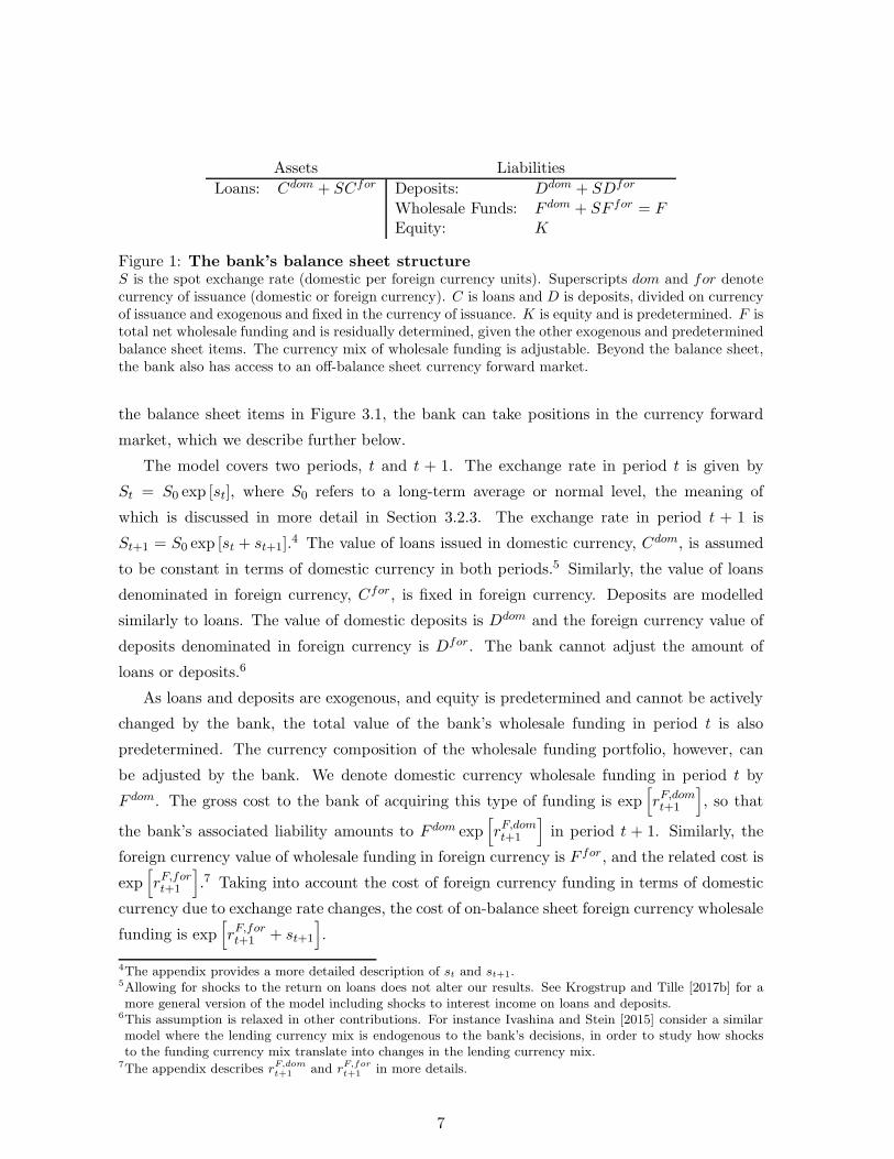
Figure 3.1 is a snapshot of the model’s bank balance sheet. There is only one foreign currency,

which we think of as the USD. The exchange rate between the domestic and the foreign

currency, in terms of units of local currency per unit of foreign currency, is denoted by S.

The bank’s assets are loans, C, issued either in domestic or in foreign currency. Its liabilities

include domestic and foreign currency deposits and wholesale funding, D and F , and equity

issued in domestic currency, K.3 Wholesale funding figures on the liabilities side of the

balance sheet, and since it is net of wholesale lending, it can turn negative. In addition to

2See Christensen and Krogstrup [2016] for an example of how bank deposits can respond autonomously tothe portfolio choice of a bank’s customers, and Choi and Choi [2016] for how banks tend to adjust wholesalefunding to shocks in deposit funding empirically.

3No equity is issued in foreign currency.

6

Assets Liabilities

Loans: Cdom + SCfor Deposits: Ddom + SDfor

Wholesale Funds: F dom + SF for = FEquity: K

Figure 1: The bank’s balance sheet structureS is the spot exchange rate (domestic per foreign currency units). Superscripts dom and for denotecurrency of issuance (domestic or foreign currency). C is loans and D is deposits, divided on currencyof issuance and exogenous and fixed in the currency of issuance. K is equity and is predetermined. F istotal net wholesale funding and is residually determined, given the other exogenous and predeterminedbalance sheet items. The currency mix of wholesale funding is adjustable. Beyond the balance sheet,the bank also has access to an off-balance sheet currency forward market.

the balance sheet items in Figure 3.1, the bank can take positions in the currency forward

market, which we describe further below.

The model covers two periods, t and t + 1. The exchange rate in period t is given by

St = S0 exp [st], where S0 refers to a long-term average or normal level, the meaning of

which is discussed in more detail in Section 3.2.3. The exchange rate in period t + 1 is

St+1 = S0 exp [st + st+1].4 The value of loans issued in domestic currency, Cdom, is assumed

to be constant in terms of domestic currency in both periods.5 Similarly, the value of loans

denominated in foreign currency, Cfor, is fixed in foreign currency. Deposits are modelled

similarly to loans. The value of domestic deposits is Ddom and the foreign currency value of

deposits denominated in foreign currency is Dfor. The bank cannot adjust the amount of

loans or deposits.6

As loans and deposits are exogenous, and equity is predetermined and cannot be actively

changed by the bank, the total value of the bank’s wholesale funding in period t is also

predetermined. The currency composition of the wholesale funding portfolio, however, can

be adjusted by the bank. We denote domestic currency wholesale funding in period t by

F dom. The gross cost to the bank of acquiring this type of funding is exp[

rF,domt+1

]

, so that

the bank’s associated liability amounts to F dom exp[

rF,domt+1

]

in period t + 1. Similarly, the

foreign currency value of wholesale funding in foreign currency is F for, and the related cost is

exp[

rF,fort+1

]

.7 Taking into account the cost of foreign currency funding in terms of domestic

currency due to exchange rate changes, the cost of on-balance sheet foreign currency wholesale

funding is exp[

rF,fort+1 + st+1

]

.

4The appendix provides a more detailed description of st and st+1.5Allowing for shocks to the return on loans does not alter our results. See Krogstrup and Tille [2017b] for amore general version of the model including shocks to interest income on loans and deposits.

6This assumption is relaxed in other contributions. For instance Ivashina and Stein [2015] consider a similarmodel where the lending currency mix is endogenous to the bank’s decisions, in order to study how shocksto the funding currency mix translate into changes in the lending currency mix.

7The appendix describes rF,domt+1 and r

F,fort+1 in more details.

7

Banks also participate in the foreign currency swap market (Fender and McGuire [2010]).

We include this dimension through a forward exchange rate contract. The contract pays off

the forward rate Tt+1 = S0 exp [tt+1] units of domestic currency per foreign currency in period

t + 1, which is known in period t. The realized cost in period t + 1 of this covered foreign

funding through the swap market is thus exp[

rF,fort+1 + tt+1 − st

]

. As all terms are fully known

in period t, the covered foreign currency funding position entails no risk, and it is therefore

directly comparable to domestic currency funding in its risk profile. If tt+1 − st < rF,domt+1 −

rF,fort+1 , the cost of swapped funding is lower than the cost of domestic wholesale funding. In

the absence of other costs, this implies an unlimited risk-free arbitrage opportunity, and the

only equilibrium would be for the cost of domestic and covered foreign funding sources to

be equalized. There is, however, occasionally large and persistent deviations from covered

interest parity, in particular since the global financial crisis. The fact that banks do not

take unlimited positions suggests the presence of additional costs in foreign currency swap

markets (Ivashina and Stein [2015]). Such costs could be time varying risk premiums of

specific financial institutions or sectors, constraints on the balance sheet capacity of swap

market participants, and constraints on counterparty risk taking (Du et al. [2017], Borio

et al. [2016], Avdjiev et al. [2016b]). We include such costs in the model by assuming that

positions in the forward contract entail a balance sheet cost which is quadratic in the amount

of positions the bank takes. In a fully specified global equilibrium model, the presence of

such costs would be the driver of deviations from covered interest parity in the first place. In

our partial equilibrium model, however, we assume that each bank takes the deviation from

covered interest parity as given.

The presence of risk-free arbitrage through covered foreign currency borrowing, with a

marginally increasing balance sheet cost associated with it, gives banks an incentive to engage

in covered foreign currency borrowing up to the point where costs outweigh the risk-free

benefit. This part of foreign currency funding is driven purely by the risk free return and

the balance sheet costs, and not by a risk-return trade-off or a desire to change exposure to

risk. Risk exposure is fully managed in the uncovered foreign currency funding market. As

we only observe total foreign currency funding in the data, and not covered and uncovered

foreign currency funding individually, it is important to include the drivers of both types of

funding to allow us to take the implications of the model to the data.

The total payoff in period t+ 1 of buying G units of the forward contract is:

G (Tt+1 − St+1)−αt+1

2(G)2

where the balance sheet cost term αt+1 is presented in more details in the appendix.

8

3.2 Solution of the model

3.2.1 Optimality conditions

The bank is initially endowed with an equity position Kt in domestic currency:

Kt = Cdom−Ddom

− F dom + St

[

Cfor−Dfor

− F for]

We assume that the bank cannot raise new equity within the two periods. The bank’s

equity in period t+1, Kt+1, then reflects the overall changes in the values of loans, deposits,

wholesale funding, and forward exchange rate contract payoff:

Kt+1 = Cdom−Ddom

− F dom exp[

rF,domt+1

]

+St exp [st+1][

Cfor−Dfor

− F for exp[

rF,fort+1

]]

+G (Tt+1 − St+1)−αt+1

2(G)2

A bank will choose its wholesale funding currency mix—and hence its total exposure to

currency risk—according to the risk management framework employed, such as a Value-At-

Risk framework as discussed in Adrian and Shin [2014], in addition to regulatory constraints

on risk taking and other factors. It is out of the scope of this paper to model such factors in

a complete sense. Instead, we follow the literature and note that the presence of risk, moral

hazard and regulatory rules can imply a convex payoff schedule for the bank (e.g. Adrian and

Duarte [2016], Nuno and Thomas [2017]). As an approximation, we assume that the bank

maximizes a CRRA expected utility function of equity in the final period:

U =1

1− γEt (Kt+1)

1−γ

The optimization takes place subject to the constraint that overall wholesale funding is

given initially. Combining the first-order conditions with respect to the wholesale funding in

domestic and foreign currency, we get the standard result that the bank will choose uncovered

foreign currency funding to the point where the expected discounted excess returns between

the domestic and foreign currency funding are zero:

0 = E (Kt+1)−γ

[

exp[

st+1 + rF,fort+1

]

− exp[

rF,domt+1

]]

(1)

The first-order conditions with respect to the holdings of the forward contract imply

that the bank will choose covered foreign currency funding to the point where the expected

9

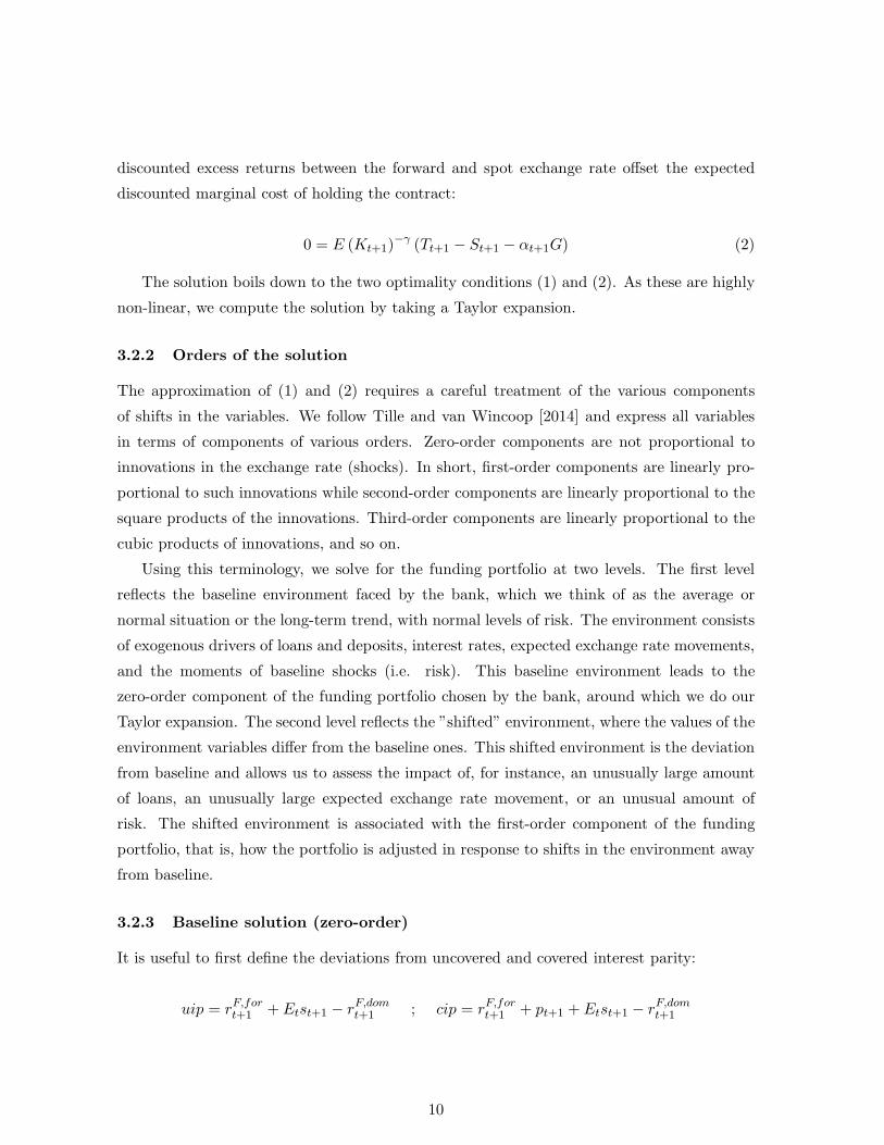
discounted excess returns between the forward and spot exchange rate offset the expected

discounted marginal cost of holding the contract:

0 = E (Kt+1)−γ (Tt+1 − St+1 − αt+1G) (2)

The solution boils down to the two optimality conditions (1) and (2). As these are highly

non-linear, we compute the solution by taking a Taylor expansion.

3.2.2 Orders of the solution

The approximation of (1) and (2) requires a careful treatment of the various components

of shifts in the variables. We follow Tille and van Wincoop [2014] and express all variables

in terms of components of various orders. Zero-order components are not proportional to

innovations in the exchange rate (shocks). In short, first-order components are linearly pro-

portional to such innovations while second-order components are linearly proportional to the

square products of the innovations. Third-order components are linearly proportional to the

cubic products of innovations, and so on.

Using this terminology, we solve for the funding portfolio at two levels. The first level

reflects the baseline environment faced by the bank, which we think of as the average or

normal situation or the long-term trend, with normal levels of risk. The environment consists

of exogenous drivers of loans and deposits, interest rates, expected exchange rate movements,

and the moments of baseline shocks (i.e. risk). This baseline environment leads to the

zero-order component of the funding portfolio chosen by the bank, around which we do our

Taylor expansion. The second level reflects the ”shifted” environment, where the values of the

environment variables differ from the baseline ones. This shifted environment is the deviation

from baseline and allows us to assess the impact of, for instance, an unusually large amount

of loans, an unusually large expected exchange rate movement, or an unusual amount of

risk. The shifted environment is associated with the first-order component of the funding

portfolio, that is, how the portfolio is adjusted in response to shifts in the environment away

from baseline.

3.2.3 Baseline solution (zero-order)

It is useful to first define the deviations from uncovered and covered interest parity:

uip = rF,fort+1 + Etst+1 − rF,domt+1 ; cip = rF,fort+1 + pt+1 + Etst+1 − rF,domt+1

10

where pt+1 is the forward premium.8 Positive values indicate that funding in foreign currency

is more expensive than funding in the domestic currency. This can reflect interest rate spreads,

expected exchange rate movements, and the expected forward premium (for the covered

interest parity).

We first solve for the baseline wholesale funding positions and forward contract holdings.

Denote the (zero-order) position in wholesale foreign currency funding by F for0 , and the

holdings of the forward contract by G0, and denote the second-order components of the

deviations from uncovered and covered interest parity by uipbaseline and cipbaseline respectively.

Further, define two measures of the net foreign currency exposure in the baseline solution:

NetOnB0 = S0

[

Cfor0 −Dfor

0 − F for0

]

; Nettot0 = NetOnB0 − S0G0 (3)

where Cfor0 and Dfor

0 are the (zero-order) values of foreign currency loans and deposits

in the baseline environment, and S0 is the (zero-order) exchange rate. NetOnB0 measures

on-balance sheet foreign currency exposure.9 This is the measure that we focus on in the

empirical application, as it is observed in the data. A positive value indicates that the bank

is long in foreign currency on its balance sheet, as the value of its total foreign currency loans

exceeds the values of its total foreign currency deposits and wholesale funding. This measure

does not take into account the part of foreign currency lending and funding that is covered in

the off-balance sheet forward market. Nettot0 is instead the broad measure that also includes

the exposure through the forward exchange rate contract.

Using this notation, the baseline solution is:

G0 =cipbaselineαbaseline

; Nettot0 = K0uipbaselineγ0σ2

fx

(4)

where αbaseline is the second-order term of the cost α of holding the forward contract, K0

is the zero-order component of equity, γ0 is the (zero-order) coefficient of risk aversion in the

baseline, and σ2fx is the second-order variance of exchange rate shocks.

The position in the forward contract, G0, reflects the deviation from covered interest

parity and the marginal cost of holding the contract. It is unaffected by risk aversion or

risk, because the forward contract in combination with spot funding positions offers risk-

free arbitrage, which the bank will exploit fully up until the cost of buying more contracts

outweigh the risk-free returns.

Given G0, Ffor0 follows from Nettot0 . The total exchange rate exposure that the bank

8uip and cip are presented in more details in the appendix.9In the general case, this measure of foreign currency exposure would include the cross interest on the threecomponents of the term. These are equal to one in baseline, however, and hence do not figure here.

11

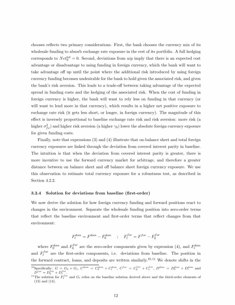
chooses reflects two primary considerations. First, the bank chooses the currency mix of its

wholesale funding to absorb exchange rate exposure in the rest of its portfolio. A full hedging

corresponds to Nettot0 = 0. Second, deviations from uip imply that there is an expected cost

advantage or disadvantage to using funding in foreign currency, which the bank will want to

take advantage off up until the point where the additional risk introduced by using foreign

currency funding becomes undesirable for the bank to hold given the associated risk, and given

the bank’s risk aversion. This leads to a trade-off between taking advantage of the expected

spread in funding costs and the hedging of the associated risk. When the cost of funding in

foreign currency is higher, the bank will want to rely less on funding in that currency (or

will want to lend more in that currency), which results in a higher net positive exposure to

exchange rate risk (it gets less short, or longer, in foreign currency). The magnitude of this

effect is inversely proportional to baseline exchange rate risk and risk aversion: more risk (a

higher σ2fx) and higher risk aversion (a higher γ0) lower the absolute foreign currency exposure

for given funding costs.

Finally, note that expressions (3) and (4) illustrate that on-balance sheet and total foreign

currency exposures are linked through the deviation from covered interest parity in baseline.

The intuition is that when the deviation from covered interest parity is greater, there is

more incentive to use the forward currency market for arbitrage, and therefore a greater

distance between on balance sheet and off balance sheet foreign currency exposure. We use

this observation to estimate total currency exposure for a robustness test, as described in

Section 4.2.2.

3.2.4 Solution for deviations from baseline (first-order)

We now derive the solution for how foreign currency funding and forward positions react to

changes in the environment. Separate the wholesale funding position into zero-order terms

that reflect the baseline environment and first-order terms that reflect changes from that

environment:

F domt = F dom

− F dom0 ; F for

t = F for− F for

0

where F dom0 and F for

0 are the zero-order components given by expression (4), and F domt

and F fort are the first-order components, i.e. deviations from baseline. The position in

the forward contract, loans, and deposits are written similarly.10,11 We denote shifts in the

10Specifically: G = G0 + Gt, Cdom = Cdom0 + Cdom

t , Cfor = Cfor0 + C

fort , Ddom = Ddom

0 + Ddomt and

Dfor = Dfor0 +D

fort .

11The solution for Ffort and Gt relies on the baseline solution derived above and the third-order elements of

(13) and (14).

12

deviations from uncovered and covered interest parity away from baseline by uipdeviation and

cipdeviation respectively, with the exact expressions given in the appendix. Positive values

indicate that funding in the foreign currency is more expensive, relative to its cost differential

in the baseline environment.

Using these expressions, the holdings of the forward contract reflect the deviation from

covered interest parity and the hedging cost (all relative to their baseline values):

Gt =cipdeviationαbaseline

−G0αdeviation

αbaseline

(5)

where αdeviation is the third-order component of the cost α, and reflects how the cost of

holding the forward contract differs from the baseline environment (αdeviation > 0 indicates

that the cost is higher than usual).

The first-order solution for total foreign currency funding (including the covered as well

as uncovered variety) is given by:

S0Ffort = Nettot0

(

γt + νσt+1

)

+Nettot0 st (6)

−NetOnB0

Nettot0

K0st + S0C

fort − S0D

fort

−

K0

γ0

uipdeviationσ2fx

− S0

(

cipdeviationαbaseline

−G0αdeviation

αbaseline

)

The first-order solution (6) is expressed in terms of deviations from baseline values, for a

given exchange rate S0 (i.e. deviations due to valuation effects of exchange rate shifts away

from baseline are not included). The funding position in foreign currency can exceed its

baseline value (F fort > 0, meaning a larger foreign currency liability position or a smaller

foreign currency asset position) for a number of reasons.

The first term in the first line in (6) is the focus of this paper. It confirms that the

effect of risk and risk aversion on foreign funding depends qualitatively on baseline balance

sheet features. νσt+1 > 0, which captures shifts in exchange rate variance away from baseline,

indicates that risk is elevated relative to baseline, while γt > 0 reflects an environment where

risk aversion is elevated. Higher risk and/or higher risk aversion leads the bank to reduce

its exposure to exchange rate risk. A key feature is that the impact on foreign currency

funding depends on the pre-existing net foreign currency exposure. If the bank is long in

foreign currency (Nettot0 > 0) in the baseline, reducing the risk exposure requires the bank

to increase its foreign currency wholesale funding. By contrast, foreign currency wholesale

funding is reduced if the baseline net position is short (Nettot0 < 0). This is the central result

13

that we are testing in this paper.

The second term in the first line contains a standard portfolio rebalancing result as also

found in the previous literature (e.g. Hau and Rey [2008]). Foreign wholesale funding adjusts

to rebalance the direct impact of the exchange rate on the currency exposure through valuation

effects. st indicates how the initial exchange rate differs from the baseline value, with st > 0

indicating that the foreign currency is stronger than in the baseline environment. If the

bank holds a long foreign currency position in the baseline (Nettot0 > 0), the stronger foreign

currency raises the domestic currency value of the net position. This is offset by additional

funding in foreign currency.

The first term in the second line also contains the exchange rate in period t, and captures

a risk-taking channel arising from balance sheet valuation gains and losses akin to the risk

taking channel of international monetary policy transmission as described in Bruno and Shin

[2013]. Consider a situation where the bank has a long foreign currency position on balance

sheet in the baseline (NetOnB0 > 0).12 A strengthening of the foreign currency in the first

period (st > 0) generates a capital gain for the bank (before the forward contract kicks in),

and higher equity in period t + 1. All else equal, this puts the bank on a part of its utility

where marginal utility is reduced. The bank is thus willing to take on more risk. If the

baseline foreign currency exposure is long (Nettot0 > 0), taking extra risk is achieved through

a reduction of foreign currency funding (F fort < 0). Our model thus shows that the impact of

the risk taking channel depends on the initial net foreign currency exposure. The channel is

distinct from the direct impact of exchange rate exposure presented in the first line. Notice

that the impact of this term on wholesale foreign currency funding also depends on the equity

position of the bank (K0), which we do not observe empirically.

The last two terms in the second line capture the effect of deviations in foreign currency

loans and deposits from baseline on wholesale foreign currency funding. The terms Cfort and

Dfort indicate if the value of loans and deposits denominated in foreign currency deviate from

the baseline environment. The bank’s long foreign exchange position is increased when there

are more loans (Cfort > 0) or fewer deposits (Dfor

t < 0) denominated in foreign currency, and

this is offset by higher foreign currency wholesale funding.

The third line in (6) captures the drivers of wholesale foreign currency funding related

to interest rates. Uncovered funding will respond directly to changes in the deviation from

uncovered interest parity uipdeviation > 0, following expression (4). Covered funding will be

unresponsive to changes in risk factors, as also illustrated by expression (4), but will instead

12The fact that it is the on-balance sheet exposure that matters to the valuation again is an artifact of ourmodeling choices, and has to do with the way we model the forward rate as a function of the baseline spotexchange rate and not the shifted one.

14

be driven by the excess risk-free return that can be made on covered foreign currency funding

relative to domestic currency funding (the deviations from covered interest parity) and the

balance sheet costs associated with positions in the forward contract. If the deviation from

covered interest parity increases (cipdeviation > 0) or the cost of holding the forward contract

goes up (αdeviation > 0), covered foreign currency wholesale funding drops.

The third line also makes clear that the response of total foreign wholesale funding to

funding costs depends on baseline variables specific to the bank (balance sheet structure

and behavior), suggesting that these terms should enter a panel regression allowing for the

parameter estimates to vary across countries. We do this in robustness checks.

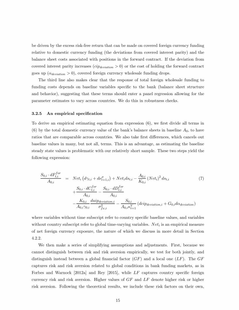
3.2.5 An empirical specification

To derive an empirical estimating equation from expression (6), we first divide all terms in

(6) by the total domestic currency value of the bank’s balance sheets in baseline A0, to have

ratios that are comparable across countries. We also take first differences, which cancels out

baseline values in many, but not all, terms. This is an advantage, as estimating the baseline

steady state values is problematic with our relatively short sample. These two steps yield the

following expression:

S0,i · dFfort,i

A0,i= Neti

(

dγt,i + dνσt+1,i

)

+Netidst,i −A0,i

K0,i(Neti)

2 dst,i (7)

+S0,i · dC

fort,i

A0,i−

S0,i · dDfort,i

A0,i

−

K0,i

A0,iγ0,i

duipdeviation,iσ2fx,i

−

S0,i

A0,iκVt+1

(dcipdeviation,i +G0,idαdeviation)

where variables without time subscript refer to country specific baseline values, and variables

without country subscript refer to global time-varying variables. Neti is an empirical measure

of net foreign currency exposure, the nature of which we discuss in more detail in Section

4.2.2.

We then make a series of simplifying assumptions and adjustments. First, because we

cannot distinguish between risk and risk aversion empirically, we test for both jointly, and

distinguish instead between a global financial factor (GF ) and a local one (LF ). The GF

captures risk and risk aversion related to global conditions in bank funding markets, as in

Forbes and Warnock [2012a] and Rey [2015], while LF captures country specific foreign

currency risk and risk aversion. Higher values of GF and LF denote higher risk or higher

risk aversion. Following the theoretical results, we include these risk factors on their own,

15

and interacted with net currency exposure, in the estimating equation.

Second, the model indicates that the parameters for the risk taking channel of exchange

rate valuation effects and those of uip and cip depend on country specific features (such as

bank equity and country specific average risk factors). We include them with joint param-

eter estimates in the baseline specification to simplify, but check robustness to allowing the

parameter estimates to vary across countries.

Third, the cost of engaging in foreign exchange swap contracts, α, is not empirically

observable and is hence not included in the regressions. α is likely to be correlated with

deviations from CIP , as in Ivashina and Stein [2015]. If indeed we were to allow α to be

proportional to cip in the model, the two terms would collapse into one with a different

parameter. We keep this interpretation of what cip is capturing in the regression in mind

when interpreting the results. Moreover, to the extent that the balance sheet cost is common

across countries, we can capture it with time fixed effects, which pick up all factors that are

common across countries but vary over time. As a robustness text, we hence also run the

regressions with time fixed effects instead of the global factor on its own, but still including

the interaction between the global factor and net currency exposure.

Finally, we add country fixed effects to capture all time invariant country specific factors

affecting foreign currency funding decisions. Taking into account all these assumptions and

adjustments yields our main empirical estimating equation:

dF fort,i = β0 + β1 · dlog (GFt−1) + β2 ·Neti · dlog (GFt−1) (8)

+β3 · dlog (LFt−1) + β4 ·Neti · dlog (LFt−1)

+β5 · dlog (Si,t−1) + β6Neti · dlog (Si,t−1) + β7 ·Net2i · dlog (Si,t−1)

+β8 ·Neti + β9 ·Net2i

+β10 · dCfort,i + β11 · dD

fort,i

+β12 · duipi,t−1 + β13 · dcipi,t−1

+µi + ǫi,t

where dF fort,i = Si,t−1dF

fort,i /Ai,t is the valuation adjusted change in net foreign currency

wholesale funding as a share of total bank assets, dCfort,i = Si,t−1dC

fort,i /Ai,t is the valuation

adjusted change in foreign currency assets net of wholesale assets as a share of total bank

assets, and dDfort,i = Si,t−1dD

fort,i /Ai,t is the valuation adjusted change in foreign currency

liabilities net of wholesale liabilities as a share of total bank assets.

The model analyzes the bank’s demand for foreign currency wholesale funding, taking the

16

supply side as well as domestic and global prices of funding as exogenous. It is possible that

changes in demand also affect prices and supply, giving rise to endogeneity, a common problem

in the literature. We follow the standard approach of lagging all explanatory variables by one

quarter (e.g. Cerutti et al. [2016]). Given that there is some persistence in bank balance

sheet dynamics and in the explanatory variables, one should bear in mind that lagging may

not fully alleviate endogeneity concerns.

The model implies that β1, β2, β4, β6 and β10 are positive, and β7, β11, β12 and β13 are

negative. There are no priors for the signs of the remaining parameter estimates.

4 The data

4.1 Dependent variable

For bank balance sheet data, we rely on the Swiss Franc Lending Monitor (SFLM) database.

This database is maintained by the Swiss National Bank and contains data from 20 partici-

pating European central banks.13 We include the 16 of these countries, that have sufficiently

complete data, in our sample.14 Most, but not all, of the data included in the SFLM are

publicly available through national data sources. The SFLM was initiated in 2009, but some

participating countries provide data for earlier quarters as well, and we use an unbalanced

sample that starts in the first quarter of 2007.15 This allows us to cover a part of the financial

crisis period. We check robustness throughout to excluding data prior to Q2 2009, which

turns out to be important. The SFLM contains quarterly data on various components of res-

ident banks’ balance sheet positions, aggregated to the country level across all banks residing

in the country.16 All balance sheet positions are divided on currency of issuance. Specifically,

positions are divided on those issued in local currency, those issued in Swiss francs, and those

issued in other foreign currencies than the Swiss franc. These other foreign currency positions

are not broken further down into individual currencies. Assets are divided on lending and

other assets, while liability positions are divided on deposits (including repo and interbank

borrowing), own securities issuance and other liabilities. Lending and deposits are further

13Austria, Bulgaria, Czech Republic, Croatia, Denmark, Estonia, France, Germany, Greece, Hungary, Iceland,Italy, Latvia, Luxembourg, Poland, Romania, Serbia, Slovenia, Slovakia, and the United Kingdom.

14We exclude Iceland and France due to insufficient data coverage. Luxembourg is excluded as an outlier,and Poland is excluded due to incomplete data on the asset side of the balance sheet. We include data forEstonia from 2011 when it joined the euro. Estonia is hence considered a euro area country. In contrast, weinclude data for Latvia only until 2014, when it joined the euro, and we hence consider Latvia a non-euroarea country in this sample.

15The individual country charts in the appendix reflect the period covered for each country.16The data thus includes subsidiaries of foreign banks, but not foreign bank branches. Subsidiaries of foreignbanks, especially European ones, account for a very large share of the market, particularly in some EasternEuropean countries.

17

divided on resident banks and non-banks, and non-resident banks and non-banks.17 The

data structure is comparable in structure to the BIS locational banking statistics, but with a

different country coverage. In particular, the division of bank balance sheets on currencies in

the SFLM covers a broader set of European countries than the locational banking statistics,

and in particular, it includes eastern European countries.

Our dependent variable is the change in net wholesale funding in foreign currency at

constant exchange rates, as a ratio to total bank assets.18 We measure foreign currency

wholesale funding as the difference between foreign currency liabilities to non-resident bank

counterparties, minus foreign currency denominated claims on non-resident bank counterpar-

ties. Including non-bank foreign claims and liabilities does not affect the results, as these

positions are relatively small. As the SFLM quotes the value of all positions in domestic cur-

rency equivalents, we adjust for the direct valuation impact of exchange rate movements, as

these affect the domestic currency value of a position issued in foreign currency. This is easily

done for positions in Swiss francs, which are quoted explicitly in the SFLM. The adjustment

is more challenging for other foreign currency positions, for which we rely on country specific

data sources for the currency breakdown. The steps and the sources used to valuation adjust

positions are described Appendix C. A similar adjustment is made when computing the flows

of loans and non-wholesale liabilities denominated in foreign currencies.

Appendix E contains plots of the resulting net cross-border funding flows in foreign cur-

rency to bank counterparties as well as cross border flows to all counterparties and in all

currencies for each of the sample countries. We observe substantial variation across countries

and time. A pattern of particular interest is that foreign currency bank flows are of smaller

magnitude for euro area countries than for other countries. There is much less heterogeneity

in overall flows (including the ones in domestic currency). This reflects that cross border

flows in euro countries are to a larger extent denominated in euros. We thus carry out all

regressions splitting the sample into euro and non-euro area countries, a distinction that turns

out to be important.

4.2 Explanatory variables

4.2.1 Risk factors

The main explanatory variables of interest are the global and local factors capturing risk

and risk aversion. The literature proposes a host of different measures of global risk factors.

17The data does not divide positions with foreign bank counterparties on positions vis-a-vis a foreign parentbank and positions vis-a-vis an unrelated foreign bank.

18To focus on changes in positions between the domestic banking sector and the rest of the economy, we excludedomestic interbank positions from total bank assets.

18

We use quarterly growth in US broker dealer leverage, following Adrian et al. [2014], as the

baseline global risk factor. Higher leverage growth among US broker dealers is associated

with lower global risk aversion and higher liquidity within global wholesale funding markets.

This global risk factor measure is likely to be particularly relevant for international banking

flows, and this is indeed what we confirm in our empirical analysis. We multiply broker

dealer leverage growth by −1 so that an increase denotes a higher level of risk aversion or

more restrictive global financial conditions. We refer to this measure as gbdl in the following.

We also consider other measures used in the literature, such as the log of the V IX (Forbes

and Warnock [2012a], Rey [2015], Goldberg and Krogstrup [2016]), referred to as lvix in the

following, and different measures of US financial and monetary conditions, further described

in Section 5.3. We show that these alternative measures are less empirically relevant as drivers

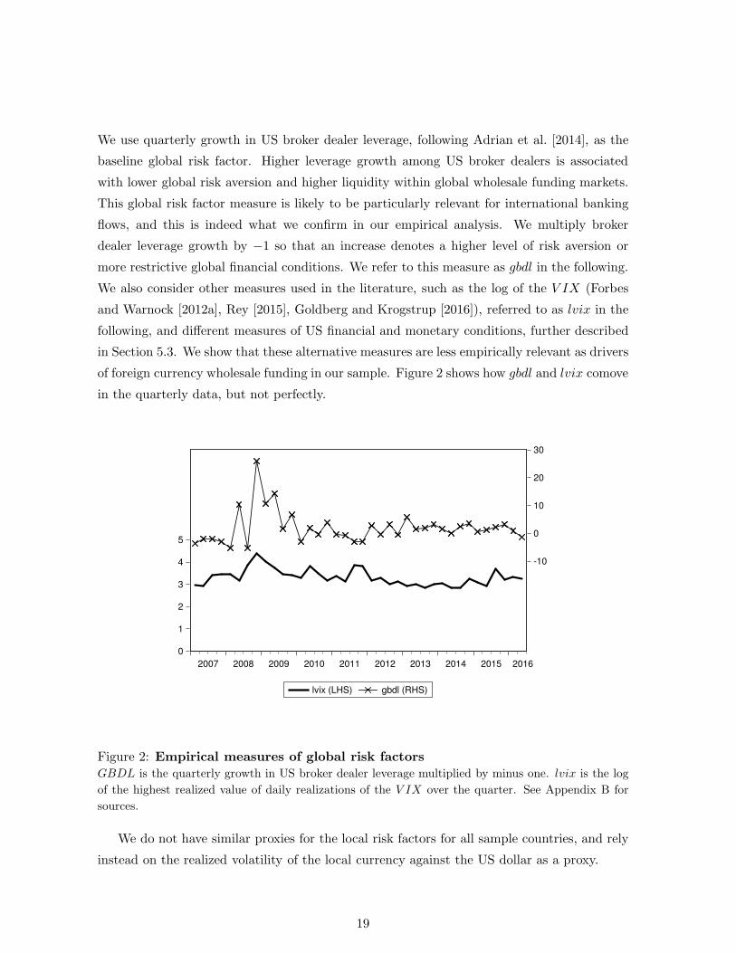
of foreign currency wholesale funding in our sample. Figure 2 shows how gbdl and lvix comove

in the quarterly data, but not perfectly.

0

1

2

3

4

5

-10

0

10

20

30

2007 2008 2009 2010 2011 2012 2013 2014 2015 2016

lvix (LHS) gbdl (RHS)

Figure 2: Empirical measures of global risk factorsGBDL is the quarterly growth in US broker dealer leverage multiplied by minus one. lvix is the log

of the highest realized value of daily realizations of the V IX over the quarter. See Appendix B for

sources.

We do not have similar proxies for the local risk factors for all sample countries, and rely

instead on the realized volatility of the local currency against the US dollar as a proxy.

19

4.2.2 Net foreign currency exposure

To test the hypothesis that net foreign currency exposure determines how banks respond to

changes in global risk conditions, we need a measure of banks’ currency exposure. The size and

sign of this exposure is driven by deviations from uip as well as initial equity, average riskiness

and risk preferences, according to expression (4). As the levels of these variables are not

observable, we instead seek to measure foreign currency exposure directly.19 The theoretical

treatment in Section 3 suggests that it is the total currency exposure, including off balance

sheet positions, which matters, but the SFLM does not report off-balance sheet exposures, and

we are not aware of other sources of data that do so consistently across countries and time.

Instead, we approximate the exposure to foreign currency by the on-balance sheet foreign

currency mismatch, which is directly observable in the SFLM. Specifically, we measure Neti

in expression (8) as foreign currency assets minus foreign currency liabilities, divided by total

bank assets.20 Neti can conceivably range from −1 (if all liabilities and no assets are in

foreign currency) to 1 (if all assets but no liabilities are in foreign currency). A positive value

indicates that the banking sector of country i has a long foreign currency exposure on its

balance sheet. Figure 3 depicts country specific sample average foreign currency exposures

for each country. Figures 9 to 11 in Appendix E illustrate the variation over time in Neti

within each of the sample countries. As time variation is substantial, we rely on the lagged

Neti for the interaction term in the regression, instead of using the country sample averages.21

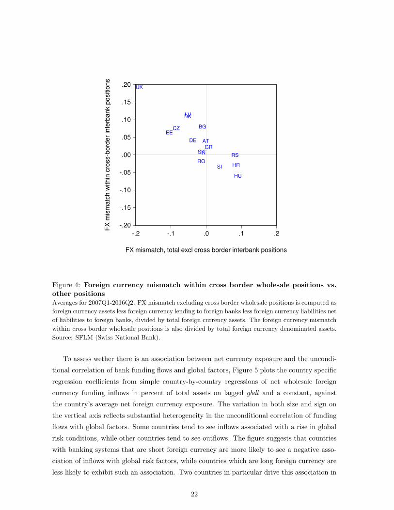
The net on balance sheet exposure is composed of the exposure within non-wholesale

funding positions and the exposure within wholesale positions. Our model illustrated that

the bank uses the currency mix of the adjustable wholesale funding to redress excessive for-

eign currency exposures within the parts of its balance sheet that it cannot adjust. The net

currency exposures in our data set are consistent with this use of wholesale funding. This is

illustrated by Figure 4, which contrasts the currency exposure in wholesale funding with the

exposure in the other components of the balance sheet. The country-specific average exposure

excluding net wholesale funding is shown on the horizontal axis, while the exposure in the

wholesale funding position is shown on the vertical axis. If banks used wholesale funding

in foreign currency to fully offset their exposure in the other positions of the balance sheet,

the dots would line up on the negative 45 degrees line. While this is not exactly the case,

we observe a clear negative association, suggesting that banks respond to the foreign cur-

19In robustness tests using the level of deviations from uip unadjusted for equity or risk as a proxy for netforeign currency exposure, we get very similar results. Not shown, but results are available upon request.

20Total bank assets exclude domestic interbank positions. Austria, Denmark and the Czech Republic do notreport other assets and liabilities. For these countries, we instead proxy the foreign currency mismatch bythe mismatch reflected in total lending and total deposits only.

21Sample average would be closer to theory, but our sample does not allow us to reasonably assess long-termunderlying structural values

20

-.06

-.04

-.02

.00

.02

.04

.06

.08

.10

EE RO CZ SK IT UK DE SI GR HU AT DK LV HR BG RS

Figure 3: Average foreign currency mismatchAverages for 2007Q1-2016Q2. Foreign currency mismatch is computed as foreign currency assets less

foreign currency liabilities divided by total bank assets net of domestic interbank positions. Source:

SFLM (Swiss National Bank).

rency exposure in their non-wholesale portfolio by taking offsetting positions in the wholesale

funding market.

21

-.20

-.15

-.10

-.05

.00

.05

.10

.15

.20

-.2 -.1 .0 .1 .2

BGCZ

HR

HU

LV

RORS

GRIT

SI

SK

EE

ATDE

DK

UK

FX mismatch, total excl cross border interbank positions

FX

mis

ma

tch

with

in c

ross-b

ord

er

inte

rba

nk p

ositio

ns

Figure 4: Foreign currency mismatch within cross border wholesale positions vs.other positionsAverages for 2007Q1-2016Q2. FX mismatch excluding cross border wholesale positions is computed as

foreign currency assets less foreign currency lending to foreign banks less foreign currency liabilities net

of liabilities to foreign banks, divided by total foreign currency assets. The foreign currency mismatch

within cross border wholesale positions is also divided by total foreign currency denominated assets.

Source: SFLM (Swiss National Bank).

To assess wether there is an association between net currency exposure and the uncondi-

tional correlation of bank funding flows and global factors, Figure 5 plots the country specific

regression coefficients from simple country-by-country regressions of net wholesale foreign

currency funding inflows in percent of total assets on lagged gbdl and a constant, against

the country’s average net foreign currency exposure. The variation in both size and sign on

the vertical axis reflects substantial heterogeneity in the unconditional correlation of funding

flows with global factors. Some countries tend to see inflows associated with a rise in global

risk conditions, while other countries tend to see outflows. The figure suggests that countries

with banking systems that are short foreign currency are more likely to see a negative asso-

ciation of inflows with global risk factors, while countries which are long foreign currency are

less likely to exhibit such an association. Two countries in particular drive this association in

22

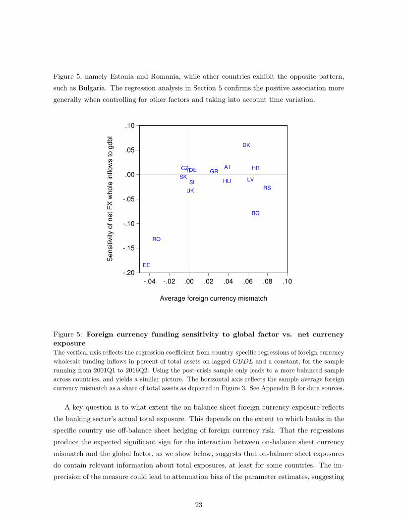
Figure 5, namely Estonia and Romania, while other countries exhibit the opposite pattern,

such as Bulgaria. The regression analysis in Section 5 confirms the positive association more

generally when controlling for other factors and taking into account time variation.

-.20

-.15

-.10

-.05

.00

.05

.10

-.04 -.02 .00 .02 .04 .06 .08 .10

BG

CZ HR

HU LV

RO

RS

GRIT

SISK

EE

ATDE

DK

UK

Average foreign currency mismatch

Se

nsitiv

ity o

f n

et

FX

wh

ole

in

flo

ws t

o g

db

l

Figure 5: Foreign currency funding sensitivity to global factor vs. net currencyexposureThe vertical axis reflects the regression coefficient from country-specific regressions of foreign currency

wholesale funding inflows in percent of total assets on lagged GBDL and a constant, for the sample

running from 2001Q1 to 2016Q2. Using the post-crisis sample only leads to a more balanced sample

across countries, and yields a similar picture. The horizontal axis reflects the sample average foreign

currency mismatch as a share of total assets as depicted in Figure 3. See Appendix B for data sources.

A key question is to what extent the on-balance sheet foreign currency exposure reflects

the banking sector’s actual total exposure. This depends on the extent to which banks in the

specific country use off-balance sheet hedging of foreign currency risk. That the regressions

produce the expected significant sign for the interaction between on-balance sheet currency

mismatch and the global factor, as we show below, suggests that on-balance sheet exposures

do contain relevant information about total exposures, at least for some countries. The im-

precision of the measure could lead to attenuation bias of the parameter estimates, suggesting

23

that actual associations could be even stronger.

As a second approach to measuring currency exposure, we note that Expressions (3) and

(4) describe the relationship between the on-balance sheet exposure and the total exposure

as a function of the deviation from covered interest parity, or NetOnB0 = Nettot0 +S0

cipbaseline

αbaseline.

Assuming that α is a constant or linearly proportional to cip, we then regress the net on-

balance sheet exposure on the deviations from covered interest parity. The residuals from

that regression are, in turn, used as an alternative proxy for the total balance sheet exposure:

Netc,tot

t = εct (9)

where εct are the residuals from the panel regression Netc,OnBt = βcipct + εct . As this approach

relies on data on deviations from covered interest parity which are quite volatile (see below),

and because other factors not included in the model that could influence the net total currency

exposure of banks, such as bank regulation of risk exposures, we use this measure of total

exposure only as a robustness check, and not as our main measure of currency exposure.22

Finally, it should be kept in mind that a dimension of banks’ exposures to foreign currency,

which we do not account for, is the indirect exposure through the credit risk of clients, which

can be associated with foreign currency risk if clients are exposed to foreign currency risk.

Banks in many European countries have issued foreign currency mortgages to clients and in

turn partly hedged these on their own balance sheet, while clients will often have not hedged

their resulting foreign currency exposure. Banks are likely to factor such exposures into their

portfolio decisions as well.

4.2.3 Other explanatory variables

Based on the model, the empirical analysis controls for a range of other explanatory variables.

We briefly discuss how these are measured here, with a more detailed description of definitions

and sources (as well as information on additional data used in robustness tests) given in

Appendix B. The flows of new loans and deposits in foreign currency, dCFX and dDFX , are

computed from the SFLM, adjusting for the valuation effect of exchange rates. The local risk

factor is measured through the intra-quarter volatility of the exchange rate vis-a-vis the US

dollar, lvol USD. The exchange rate is included in the form of the appreciation of the dollar

through the quarter, d USD. Relative funding costs in domestic and foreign currency are

proxied by deviations from uncovered interest parity, dUIP , computed as the simple interest

differential, and deviations from covered parity, dCIP . The computation of deviations from

covered interest parity is explained in more detail in Appendix B. Currency swap markets are

22See also footnote 19 on using uip is a proxy for net exposure.

24

not necessarily liquid for all these countries, giving rise to rather volatile deviations, notably

for Latvia (which accounts for the max and min observations of the dCIP recorded in Table

1, Romania and Serbia. In robustness tests not reported here, we have used averages of the

last month of the quarter instead of the last week of the quarter in order to average out some

of the volatility. The regression results are largely the same, however, and deviations from

covered interest parity are rarely significant in any case.

In robustness tests, we consider additional measures of global funding conditions, as de-

scribed in Section 5.3, as well as country growth and inflation.

Summary statistics of all regression variables are provided in Table 1.

5 Results

5.1 Full sample

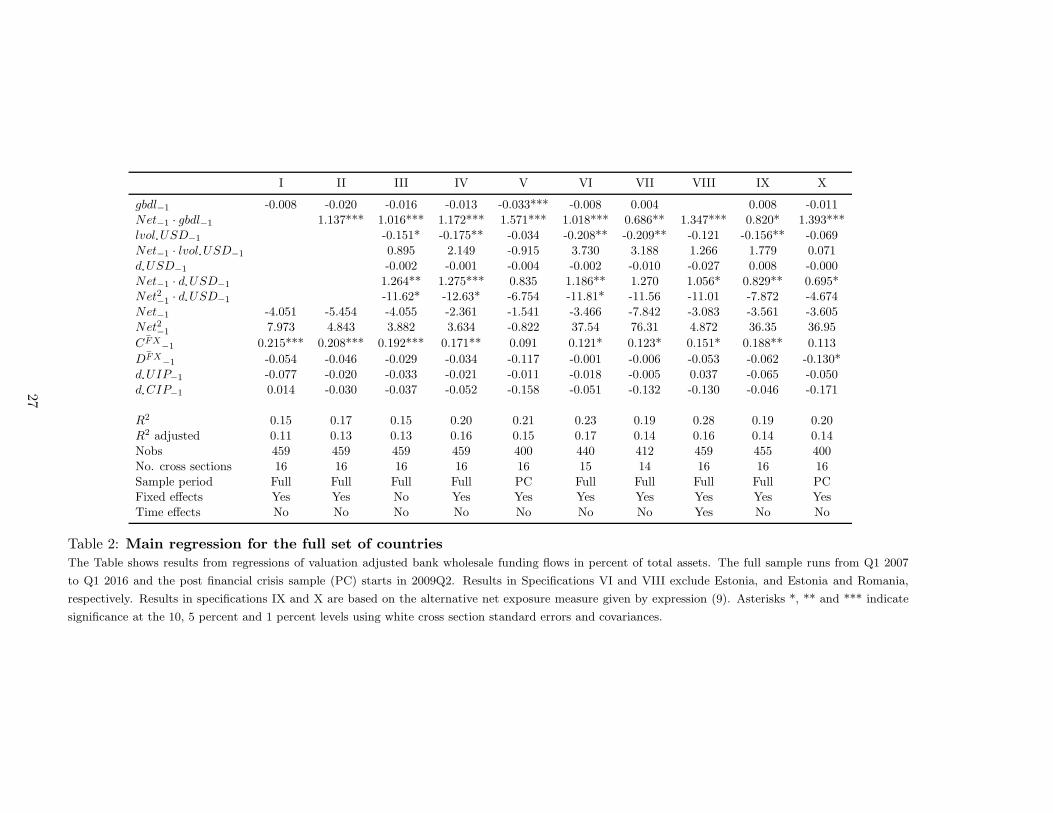
We first run the regression on the whole sample of European countries, with the results of

different specifications shown in the columns of Table 2. All specifications rely on growth

in US broker dealer leverage as the global factor. In Section 5.3, we consider alternative

measures of the global factor including the V IX, and show that growth in US broker dealer

leverage is the most relevant one for this sample of countries and the type of bank flows we

are considering.

Column I shows that the global factor is not significant when it enters on its own and

without other risk factors. This stands in contrast with the earlier literature, but is in line

with the findings of Avdjiev et al. [2016c] that the V IX has not been a significant driver of

cross-border banking flows in recent years, in contrast to earlier years. Column II shows that

the global factor is significant in interaction with foreign currency exposure. A higher risk

factor, as measured by an increase in gbdl, reduces foreign currency funding, but increases it

for banks that have a long exposure, in line with the theory. This finding is consistent across

the different specifications in columns II to X.

Turning to the other explanatory variables, higher exchange rate volatility, as a measure of

local risk factors, reduces funding, but this impact does not depend significantly on currency

exposure. Global risk factors seem to be more important in driving perceived foreign currency

risk than local factors, for the banking sectors in the sample that we consider.

Realized exchange rate movements enter significantly and with the right signs through

portfolio rebalancing in response to valuation effects (interaction term with net exposure),

and through the risk taking channel (interaction term with the square of net exposure). We

also find that wholesale funding reacts to the flows of loans granted in foreign currency, with

the positive coefficient indicating a partial offsetting of new exchange rate exposure. No such

25

Variable Mean Median Max Min Std. Dev. Obs

Euro Area SampledFFX -0.04 -0.06 5.01 -5.65 0.80 211dF l -0.10 -0.09 8.50 -7.86 1.55 212Net 0.01 0.00 0.06 -0.08 0.03 216lvol USD -1.48 -1.44 0.20 -3.24 0.73 236d USD 1.47 -0.54 11.71 -9.63 4.73 254dCFX -0.07 -0.06 4.93 -5.26 0.84 212dDFX -0.08 -0.05 1.94 -2.26 0.55 208dUIP -0.01 0.02 1.16 -2.04 0.46 280dCIP -0.017 0.005 1.14 -1.38 0.34 263

Non-Euro Countries SampledFFX -0.14 -0.21 7.10 -4.45 1.58 284dF l 0.05 0.03 3.42 -2.50 0.76 298Net 0.03 0.04 0.16 -0.15 0.05 303lvol USD -1.21 -1.21 1.37 -3.23 0.81 313d USD 0.81 -0.06 20.79 -16.72 5.91 345dCFX 0.23 0.04 15.84 -15.45 2.37 298dDFX 0.30 0.07 16.79 -4.62 2.23 298dUIP 0.02 0.05 5.74 -7.02 1.26 348dCIP 0.001 -0.008 4.50 -4.20 0.69 318

Global Factorsgbdl 1.98 1.24 25.96 -5.22 5.71 39lvix 3.31 3.25 4.39 2.83 0.37 39

Table 1: Data and descriptive statisticsThe euro area sample includes Austria, Estonia (post euro), Germany, Greece, Slovakia and Slovenia. The

non-euro sample includes Bulgaria, Croatia, Czech Republic, Denmark, Hungary, Latvia (before joining the

euro), Romania, Serbia and the UK. lvol USD and lD USD are the same for all euro area countries and the

number of independent observations would be 39 for these variables in the euro area sample. All variables are

expressed in percentage or percentage points, except for Net, which is expressed as a ratio of total bank assets.

The sample is unbalanced and runs from Q1 2007 to Q1 2016. Number of observations include all individual

observations of the given variable during the sample period. The appendix presents data sources, definitions

and computations in more detail.

26

I II III IV V VI VII VIII IX X

gbdl−1 -0.008 -0.020 -0.016 -0.013 -0.033*** -0.008 0.004 0.008 -0.011

Net−1 · gbdl−1 1.137*** 1.016*** 1.172*** 1.571*** 1.018*** 0.686** 1.347*** 0.820* 1.393***

lvol USD−1 -0.151* -0.175** -0.034 -0.208** -0.209** -0.121 -0.156** -0.069

Net−1 · lvol USD

−1 0.895 2.149 -0.915 3.730 3.188 1.266 1.779 0.071d USD

−1 -0.002 -0.001 -0.004 -0.002 -0.010 -0.027 0.008 -0.000Net

−1 · d USD−1 1.264** 1.275*** 0.835 1.186** 1.270 1.056* 0.829** 0.695*

Net2−1 · d USD

−1 -11.62* -12.63* -6.754 -11.81* -11.56 -11.01 -7.872 -4.674Net

−1 -4.051 -5.454 -4.055 -2.361 -1.541 -3.466 -7.842 -3.083 -3.561 -3.605Net2

−1 7.973 4.843 3.882 3.634 -0.822 37.54 76.31 4.872 36.35 36.95¯CFX

−1 0.215*** 0.208*** 0.192*** 0.171** 0.091 0.121* 0.123* 0.151* 0.188** 0.113¯DFX

−1 -0.054 -0.046 -0.029 -0.034 -0.117 -0.001 -0.006 -0.053 -0.062 -0.130*d UIP

−1 -0.077 -0.020 -0.033 -0.021 -0.011 -0.018 -0.005 0.037 -0.065 -0.050d CIP

−1 0.014 -0.030 -0.037 -0.052 -0.158 -0.051 -0.132 -0.130 -0.046 -0.171

R2 0.15 0.17 0.15 0.20 0.21 0.23 0.19 0.28 0.19 0.20R2 adjusted 0.11 0.13 0.13 0.16 0.15 0.17 0.14 0.16 0.14 0.14Nobs 459 459 459 459 400 440 412 459 455 400No. cross sections 16 16 16 16 16 15 14 16 16 16Sample period Full Full Full Full PC Full Full Full Full PCFixed effects Yes Yes No Yes Yes Yes Yes Yes Yes YesTime effects No No No No No No No Yes No No

Table 2: Main regression for the full set of countriesThe Table shows results from regressions of valuation adjusted bank wholesale funding flows in percent of total assets. The full sample runs from Q1 2007

to Q1 2016 and the post financial crisis sample (PC) starts in 2009Q2. Results in Specifications VI and VIII exclude Estonia, and Estonia and Romania,

respectively. Results in specifications IX and X are based on the alternative net exposure measure given by expression (9). Asterisks *, ** and *** indicate

significance at the 10, 5 percent and 1 percent levels using white cross section standard errors and covariances.

27

offset is seen in response to movements in deposits. We find no evidence that funding reacts

short-term to deviations from interest parity, with the coefficients on changes in uip and cip

deviations both insignificant.

The results are sensitive to the sample considered (with the exception of the role of the

global risk factor), as many coefficients lose significance when we exclude the crisis period

(column V and X, where we only consider observations from 2009Q2 on).

The salient result from Table 2 is the significance of gbdl interacted with exchange rate

exposure. While gbdl also matters on its own in some specifications, its impact is primarily

driven by the interaction in terms of magnitude. Consider a one standard deviation increase

in gbdl (an increase of about 6). Using the estimates of column IV, this leads to an increase

in foreign currency wholesale funding of 0.62% of assets in a country with an initial net long

foreign currency exposure of 10% of assets,23 but a contraction of foreign currency wholesale

funding of 0.78% of total assets if the country initially has a net short exposure of 10%.24

This result is robust to changes in the specification, net exposure measure, and sample

period; notably to whether fixed effect are included (columns III, IV and VIII), to using the

alternative net exposure measure given by Equation (9) (columns IX and X)25, to allowing for

the parameter estimates of deviations from interest parity conditions to vary across countries

(Table 6 in the appendix)26, and to the inclusion of a number of additional control variables

such as inflation, growth and US financial and monetary variables, as shown in Table 7 in

the appendix. The effect of gbdl interacted with net currency exposure is stronger when

the crisis period is omitted (column V and X in Table 2). Column VI in Table 2 shows

that the result is not driven by Estonia and Romania alone, the two countries with the

most clearly negative association between foreign currency exposure and the country specific

unconditional sensitivity of net foreign currency funding to gbdl in Figure (5), although the

parameter estimate becomes smaller without these countries in the sample (column VII). The

specific sample of countries matters, however, and we consider this next.

5.2 Euro area vs. other European countries

Since euro area countries and non-euro countries differ strongly in their currency denomi-

nation of cross border bank funding flows, we run the regressions separately for these two

sub-samples. The results are displayed in Table 3, where we again focus on the growth in

23−0.013 · 6 + 1.172 · 0.1 · 6 = 0.46%

24−0.013 · 6− 1.172 · 0.1 · 6 = −0.68%

25The results are also robust to using the lagged value of the level of the deviation from uip as an alternativemeasure of net foreign currency exposure, following expression (4). Not shown but results are available onrequest.

26In robustness tests not show, we also allow the parameter estimates of the risk taking term for foreigncurrency appreciation to vary across countries, with no implications for the results.

28

broker dealer leverage as a proxy for the global factor, and include country fixed effects in all

specifications.

The global factor is not significant for either group when entered alone (columns I and

V). It is however significant when interacted with the net foreign currency exposure for non-

euro countries (column II), but not for euro countries (column VI). The significance of the

interacted global factor is robust to the inclusion of additional controls for countries outside

the euro area (columns III and IV). It is also robust to the countries included in the sample.

Excluding Romania (column V) as a possible outlier reduces significance somewhat but the

results remain, and jointly excluding Denmark and the UK, or sequentially excluding any

other country, does not change the sign and significance of the interaction term (not shown).

The pattern is quite different in the sample of euro area countries. Estonia is an outlier that

strongly drives the results, and we therefore exclude it from the main euro sample in columns

VI to IX, whereas columns X and XI illustrate the results including Estonia. The interaction

term of the global factor with net currency exposure is never significant. The global factor is

marginally significant and positive when entered on its own in the post-crisis sample period

(column IX). A positive coefficient would be in line with theory, as without Estonia, euro

countries are largely long foreign currency, which would predict a greater inflow as global risk

conditions tighten. The data do not allow us to confirm this association, however. The lack

of significance of the interaction term between the global factor and exchange rate exposure

in the euro area sub-sample is quite robust.

As already noted, foreign currency funding is a marginal activity for euro-area countries,

both in terms of level and first-differences. The cross-border flows of these countries are thus

predominantly in domestic currency, and these are not included in the main specification.

For completeness, we therefore also run the regressions using net wholesale funding flows

denominated in domestic currency. The results are shown in the appendix, Table 8.27 This

change in currency denomination of cross border flows, as expected, leads to a lower fit of

the regression. Moreover, the global factor remains insignificant as a driver of local currency

flows in the euro area.28

Other drivers of foreign currency funding inflows also behave differently across euro and

non-euro countries. There is some evidence of a role for the local risk factor (exchange

27For comparability with the previous results for the euro sub-sample, we have excluded Estonia from the eurosample, but the exclusion does not matter for the results in this specification.

28Interestingly, it is significant and with the right sign when interacted with exchange rate exposure in thenon-euro sample. The regressions show other interesting results that are not the focus of this paper. Forexample, the coefficient on the deviation from uncovered interest parity is significant and negative in thefull and euro sub-samples, which is not the case for foreign currency flows. Deviations from covered interestparity are significant and positive in full sample, indicating perhaps some substitution effects between foreignand domestic currency wholesale funding.

29

Non-Euro Countries Euro Area Countries

I II III IV V VI VII VIII IX X XIgbdl

−1 -0.013 -0.032 -0.010 -0.076*** 0.012 0.004 0.005 0.005 0.014* 0.001 0.014Net

−1 · gbdl−1 1.167*** 1.039*** 2.096*** 0.621* -0.310 -0.210 -0.681 -0.213 -0.580lvol USD

−1 -0.425** -0.116 -0.465** -0.011 -0.014 -0.061 -0.034Net

−1 · lvol USD−1 5.282 1.719 5.389 0.682 0.137 2.772 1.839

d USD−1 -0.003 -0.015 -0.018 0.004 0.004 0.005 0.004

Net−1 · d USD

−1 1.082** 0.942 1.166 1.833** 1.711** 0.308 0.193Net2

−1 · d USD−1 -10.462 -6.641 -9.410 -34.72** -34.34** -0.136 -1.897

Net−1 -7.649 -8.799*** -2.384 -9.822 -7.621 3.391 4.319 5.016 5.013 38.04*** 41.77***

Net2−1 37.22 31.80 42.55 84.39 97.05 -94.22 -100.8 -94.17 -86.09 -796.6*** -796.3***

¯CFX−1 0.183*** 0.180*** 0.137* 0.072 0.144** -0.087 -0.087 -0.095 -0.146 -0.100 -0.127

¯DFX−1 -0.022 -0.014 -0.019 -0.072 -0.029 -0.087 -0.087 -0.042 -0.012 -0.088 -0.115

d UIP−1 -0.081 -0.023 -0.032 -0.028 -0.012 -0.140** -0.141** -0.174*** 0.004 -0.117 0.134

d CIP−1 0.013 -0.045 -0.059 -0.123 -0.129 -0.074 -0.066 -0.033 -0.155 0.056 -0.012

R2 0.18 0.21 0.25 0.25 0.23 0.06 0.06 0.11 0.15 0.48 0.51R2 adjusted 0.13 0.17 0.19 0.17 0.16 0.00 0.00 0.01 0.05 0.43 0.45Nobs 257 257 257 221 229 183 183 183 183 202 179No. cross sections 9 9 9 9 8 6 6 6 6 7 7Sample period Full Full Full PC Full Full Full Full PC Full PCFixed effects Yes Yes Yes Yes Yes Yes Yes Yes Yes Yes Yes

Table 3: Main regression for euro and non-euro samples separatelyThe Table shows results from regressions of valuation adjusted bank wholesale funding flows in percent of total assets. The non-euro sample includes Bulgaria,

Croatia, Czech Republic, Denmark, Hungary, Latvia (before joining the euro), Romania, Serbia and the UK. The euro area sample includes Austria, Estonia

(post euro), Germany, Greece, Slovakia and Slovenia. The full sample runs from Q1 2007 to Q1 2016 and the post financial crisis sample (PC) starts in

2009Q2. Specification V excludes Romania, specifications VI-IX exclude Estonia. Asterisks *, ** and *** indicate significance at the 10, 5 percent and 1

percent levels, respectively, using white cross section standard errors and covariances.

30

rate volatility), as well as of the use of wholesale funding as a way to offset the change in

exposure due to realized exchange rate movements (positive coefficient on Net · d USD) and

additional foreign currency loans (positive coefficient on d ¯CFX) in non-euro countries. These

effects, however, lose significance once we exclude the crisis period (column IV). Funding

cost differentials do not play a role. Euro area net foreign currency funding inflows respond

significantly to exchange rate changes interacted with net currency exposure, and to interest

rate differentials as captured by dUIP in line with theory. These findings are sensitive to

sample period as well as sample countries included, however.

Why are the results so different for euro and non-euro countries? While we do not have

data to confirm this, one difference could be in the use of off-balance sheet hedging practises,

and hence the information contents of on-balance sheet net foreign currency exposure as

a proxy for total foreign currency exposure. Euro area banks use the euro dollar forward

market, which is likely to be a substantially more deep and liquid market than many of the

bilateral forward markets for non-euro area currencies. If this is the case, then the net foreign

currency measure we use could contain more information about actual exposures in non-euro

area countries.29

Overall, the regressions indicate that the foreign currency mismatch on bank balance

sheets affects the response of cross border bank capital flows to global risk factors, especially

in non-euro area countries. Omitting the interaction with exposure affects the estimates of

the impact of global risk factors in some countries. The result suggests that changing balance

sheet features could change the sensitivity of capital flows to global risk factors, at least in

some areas of the world.

5.3 Alternative global factor measures

The literature considers a number of alternative measures of global financial factors as drivers

of capital flows. Table 7 in the appendix shows that including such measures as explanatory

variables in the baseline regression does not affect the results for gbdl. Table 4 shows the

results for the regressions when including alternative global factor measures in place of gbdl,

for the sample of all countries.

As alternative global factor measures, we consider quarterly changes in the short-term

US real interest rate (3-month money market rate less inflation)30, the quarterly change in

the term spread (10-year treasury yield less the 3-month money market rate), the log of the

29In future extensions, this conjecture would be investigated by looking at data for the depth and liquidity offorward markets across currencies.

30We also tried specifying the short-term real interest rate as the shadow federal funds rate of Wu and Xia[2016] less inflation, with no difference in the results, despite the finding that this measure is much morecorrelated with gbdl in our sample.

31

V IX, the appreciation rate of the real effective US dollar, and two alternative measures of the

US monetary policy stance. Since the Federal Funds rate has been at the zero lower bound

during the larger part of the sample period, US monetary policy has been conducted with

alternative tools, such as quantitative easing, forward guidance and the provision of swap

lines with foreign central banks. We therefore consider the growth rate in the US monetary

base and the change in the US shadow federal funds rate estimated in Wu and Xia [2016] as

measures of changes in the US monetary policy stance.

I II III IV V VIdUS RR dUS TS lvix dUS REER dUS M0 dUS SFFR

GF−1 -0.073 0.050 -0.003 0.008 -0.004 0.011

Net−1 ·GF

−1 1.664 0.709 0.087 0.137 -0.059 -1.985lvol USD

−1 -0.195** -0.219** -0.105 -0.221** -0.199** -0.208**Net

−1 · lvol USD−1 3.100 3.106 0.614 3.092 2.908 3.111

d USD−1 0.009 0.006 0.005 -0.009 0.004 0.003

Net−1 · d USD

−1 1.063 1.159* 1.082* 0.939 1.109* 1.184*Net2

−1 · d USD−1 -13.36* -12.66** -12.85* -12.53 -12.76* -12.92*

Net−1 1.758 0.303 -31.531 0.253 0.134 -0.045

Net2−1 -3.474 11.060 9.168 9.110 9.533 11.235

¯CFX−1 0.145* 0.176* 0.181** 0.181** 0.181** 0.177**

¯DFX−1 -0.009 -0.038 -0.043 -0.048 -0.049 -0.041

d UIP−1 -0.066 -0.070 -0.080 -0.074 -0.093 -0.082

d CIP−1 -0.008 -0.025 -0.016 -0.018 0.004 -0.008

R2 0.19 0.19 0.19 0.19 0.19 0.19R2 adjusted 0.13 0.13 0.14 0.14 0.13 0.13Nobs 446 459 459 459 459 459No. cross sections 16 16 16 16 16 16Sample period Full Full Full Full Full FullFixed effects Yes Yes Yes Yes Yes Yes

Table 4: Alternative global factors, all countriesThe Table shows results from regressions of valuation adjusted bank net wholesale funding flows in percent of

total assets, for the sample of all countries. The full sample period (FULL) runs from Q1 2007 to Q1 2016

and the post-crisis sample period (PC) starts in Q2 2009. Asterisks *, ** and *** indicate significance at the

10, 5 percent and 1 percent levels, respectively, using white cross section standard errors and covariances.

Table 4 shows that the alternative global factor measures considered are not significant

drivers of foreign currency wholesale funding in this sample of European banking sectors.31

Including the crisis period, or splitting the sample into euro and non-euro countries do not

change these findings (not shown). The missing role of the V IX is particularly interesting,

as this is the most frequently used measure of global risk factors in the literature. The result

31The appreciation of the broad nominal effective USD exchange rate index was also tried, without significantresults in the full sample.

32

could reflect that the V IX is derived from US equity prices which are not strictly linked

to global bank conditions. While the V IX has been found to be an important indicator of

global risk and risk aversion in the literature, it may not be the most important indicator of

the type of global risk factor that matters for foreign currency wholesale bank funding in our

particular sample.

6 Conclusion

This paper has offered a new perspective on the link between global risk factors and the cross

border foreign currency funding activity of banks. It is often argued that when global risk

sentiment eases, banks are likely to increase their reliance on foreign currency funding. We

have shown that one cannot expect a clear unidirectional relationship between global risk and

foreign currency funding. Rather, it is important to consider how global risk affects the foreign

currency risk exposure on financial institutions’ balance sheets. Easing risk conditions may

lead financial institutions to seek to increase their exposure to foreign currency risk. This

translates into lower funding in foreign currency for institutions which are long in foreign

currency (thus making the position even longer), but it translates into higher foreign currency

funding for institutions with a short exposure (thus making the position even shorter).

To illustrate these effects, we have developed a simple portfolio model of the bank’s foreign

currency wholesale funding choice, and tested its predictions empirically for cross border bank

funding flows and bank balance sheet positions in 16 European countries. When using growth

in US broker dealer leverage as a measure of the global risk factor, we have shown that the

effect of the global risk factor on wholesale funding flows depends qualitatively on the pre-

existing foreign currency exposure of the banking sector. This finding is driven mainly by

European countries that are not part of the euro area. In contrast, the relatively small foreign

currency funding positions of euro area banking sectors are not sensitive to the risk factors

we consider, which could reflect different off-balance sheet hedging practises.

Finally, our results have also shown that the most consistently relevant empirical global

risk factor for European foreign currency wholesale funding is growth in US broker dealer

leverage. Other measures used in the literature, such as the V IX, are not significant drivers

in the sample of European banking sectors we have studied.

Foreign currency risk exposure in bank balance sheets varies across countries and over

time, suggesting that the link between global factors and banks’ foreign currency funding

will also vary. We have viewed the response of banks to global risks through the prism of

portfolio risk management behavior. Other factors may be at play, such as regulatory rules.

Moreover, we have focused empirically on bank net funding flows, for which comprehensive

33

balance sheet data exist that are comparable across countries. Similar comprehensive data

are not readily available for other types of financial institutions intermediating an important

share of cross border capital flows, such as institutional investors. Other institutions may

respond differently to global factors, and we therefore cannot generalize our results to total

cross border capital flows. More research and development of better data would help further

our understanding of the link between domestic financial market structure and regulation on

the one hand, and capital flow sensitivity to global risk and hence volatility, on the other.

A better understanding could in turn help inform the design of capital flow management

measures to reduce capital flow volatility.

34

References

Tobias Adrian and Fernando M. Duarte. Financial vulnerability and monetary policy. Staff

Reports 804, Federal Reserve Bank of New York, December 2016.

Tobias Adrian and Hyun Song Shin. Procyclical Leverage and Value-at-Risk. Review of

Financial Studies, 27(2):373–403, 2014.

Tobias Adrian, Erkko Etula, and Tyler Muir. Financial intermediaries and the cross-section

of asset returns. forthcoming, The Journal of Finance, 2014.

Stefan Avdjiev and Elod Takats. Monetary policy spillovers and currency networks in cross-

border bank lending. BIS Working Papers 549, Bank for International Settlements, March

2016.

Stefan Avdjiev, Zsolt Kuti, and Elod Takats. The euro area crisis and cross-border lending to

emerging markets. Bank for International Settlements quarterly review, pages 37–47, 2012.

Stefan Avdjiev, Wenxin Du, Catherine Koch, and Hyun Song Shin. The dollar, bank lever-

age and the deviation from covered interest parity. BIS Working Papers 592, Bank for

International Settlements, November 2016a.

Stefan Avdjiev, Wenxin Du, Catherine Koch, and Hyun Song Shin. The dollar, bank leverage

and the deviation from covered interest parity. Working Papers 592, BIS, 2016b.

Stefan Avdjiev, Leonardo Gambacorta, Linda Goldberg, and Stefano Schiaffi. The shifting

drivers of international capital flows. BIS Mimeo, 2016c.

Claudio Borio, Robert Neil McCauley, Patrick McGuire, and Vladyslav Sushko. Covered inter-

est parity lost: understanding the cross-currency basis. BIS Quarterly Review, September

2016.

Franziska Bremus and Marcel Fratzscher. Drivers of structural change in cross-border banking

since the global financial crisis. Journal of International Money and Finance, 52:32 – 59,

2015.

Martin Brown and Helmut Stix. The euroization of bank deposits in Eastern Europe. paper

presented at the 59th panel meeting of economic policy, 2014.

Markus K. Brunnermeier, Stefan Nagel, and Lasse H. Pedersen. Carry Trades and Currency

Crashes. In NBER Macroeconomics Annual 2008, Volume 23, NBER Chapters, pages

313–347. National Bureau of Economic Research, Inc, April 2009.

35

Valentina Bruno and Hyun Song Shin. Capital flows and the risk-taking channel of monetary

policy. Working Paper 18942, National Bureau of Economic Research, April 2013.

Valentina Bruno and Hyun Song Shin. Cross-border banking and global liquidity. BISWorking

Papers 458, Bank for International Settlements, Aug 2014.

Valentina Bruno and Hyun Song Shin. Global dollar credit and carry trades: a firm-level

analysis. BIS Working Papers 510, Bank for International Settlements, August 2015.

Matthieu Bussiere, Julia Schmidt, and Natacha Valla. International Financial Flows in the

New Normal: Key Patterns (and Why We Should Care). CEPII Policy Brief 2016-10,

CEPII research center, March 2016.

Julian Caballero, Ugo Panizza, and Andrew Powell. The second wave of global liquidity: Why

are firms acting like financial intermediaries? CEPR Discussion Papers 10926, C.E.P.R.

Discussion Papers, November 2015.

Guillermo A. Calvo, Leonardo Leiderman, and Carmen M. Reinhart. Inflows of Capital

to Developing Countries in the 1990s. Journal of Economic Perspectives, 10(2):123–139,

Spring 1996.

Eugenio Cerutti. Drivers of cross-border banking exposures during the crisis. Journal of

Banking & Finance, 55(C):340–357, 2015.

Eugenio Cerutti, Stijn Claessens, and Andrew K Rose. How Important is the Global Financial

Cycle? Evidence from Capital Flows. CEPR Discussion Papers 12075, C.E.P.R. Discussion

Papers, June 2017.

Eugenio M Cerutti, Stijn Claessens, and Damien Puy. Push Factors and Capital Flows to

Emerging Markets; Why Knowing Your Lender Matters More Than Fundamentals. IMF

Working Papers 15/127, International Monetary Fund, June 2015.

Eugenio M Cerutti, Stijn Claessens, and Lev Ratnovski. Global Liquidity and Cross Border

Bank Flows. Economic Policy, 00(0):000–000, Jan 2016.

Nicola Cetorelli and Linda Goldberg. Global banks and international shock transmission:

evidence from the crisis. International Monetary Fund Economic Review, 59:41–46, 2011.

Nicola Cetorelli and Linda Goldberg. Follow the money: Quantifying domestic effects of

foreign bank shocks in the Great Recession. American Economic Review Papers and Pro-

ceedings, 2012.

36

Dong Boem Choi and Hyun-Soo Choi. The effect of monetary policy on bank wholesale

funding. Staff Reports 759, Federal Reserve Bank of New York, January 2016.

Jens H. E. Christensen and Signe Krogstrup. A Portfolio Model of Quantitative Easing.

Working Paper Series 2016-12, Federal Reserve Bank of San Francisco, July 2016.

Stijn Claessens and Neeltje van Horen. The impact of the global financial crisis on banking

globalization. DNB Working Papers 459, Netherlands Central Bank, Research Department,

February 2015.

Giovanni Dell’Ariccia, Luc Laeven, and Robert Maquez. Financial Frictions, Foreign Currency

Borrowing, and Systemic Risk. Manuscript 000, IMF, Dec 2016.

Wenxin Du, Alexander Tepper, and Adrien Verdelhan. Deviations from covered interest rate

parity. Working Paper 23170, National Bureau of Economic Research, February 2017.

ECB. The International Role of the Euro. Technical report, The European Central Bank,

2014.

Ingo Fender and Patrick McGuire. Bank structure, funding risk and the transmission of shocks

across countries: concepts and measurement. BIS Quarterly Review, September 2010.

Kristin Forbes and Francis Warnock. Capital flow waves: Surges, stops, flight, and restrench-

ment. Journal of International Economics, 88:235 – 251, 2012a.

Kristin J. Forbes and Francis E. Warnock. Capital flow waves: Surges, stops, flight, and

retrenchment. Journal of International Economics, 88(2):235–251, 2012b.

Marcel Fratzscher. Capital flows, push versus pull factors and the global financial crisis.

Journal of International Economics, 88(2):341–356, 2012.

Atish R. Ghosh, Mahvash S. Qureshi, Jun Il Kim, and Juan Zalduendo. Surges. Journal of

International Economics, 92(2):266–285, 2014.

Linda Goldberg and Signe Krogstrup. International Capital Flow Pressures. Paper presented

at the piie-kiep-bok conference on monetary policy options for small open economies, korea,

july 17, 2016, PIIE, Jul 2016.

Harald Hau and Helene Rey. Global portfolio rebalancing under the microscope. Technical

report, National Bureau of Economic Research, 2008.

37

IMF. How Do Changes in the Investor Base and Financial Deepening Affect Emerging Market

Economies? Chapter 2, Global Financial Stability Report, International Monetary Fund,

Apr 2014.

David S. Scharfstein Ivashina, Victoria and Jeremy C. Stein. Dollar Funding and the Lending

Behavior of Global Banks. Quarterly Journal of Economics, 130(3):1241–1281, Aug 2015.

Signe Krogstrup and Cedric Tille. What drives for foreign currency funding mix of banks?

Manuscript 000, Graduate Institute and IMF, Nov 2017a.

Signe Krogstrup and Cedric Tille. A portfolio model of cross border bank funding. mimeo,

Graduate Institute, Geneva, 2017b.

Signe Krogstrup and Cedric Tille. On the Roles of Different Foreign Currencies in European

Bank Lending, chapter in ”International Currency Exposure”. CESifo Seminar Series. MIT

Press, 1 edition, July 2017c.

Robert McCauley, Patrick McGuire, and Vladyslav Sushko. Global dollar credit: links to

US monetary policy and leverage. Working Paper 483, Bank for International Settlements,

January 2015.

Peter McQuade and Martin Schmitz. The great moderation in international capital flows: a

global phenomenon? Working Paper Series 1952, European Central Bank, August 2016.

Gian-Maria Milesi-Ferretti and Cedric Tille. The great retrenchment: International capital

flows during the global financial crisis. Economic Policy, 66:285–330, 2011.

Galo Nuno and Carlos Thomas. Bank Leverage Cycles. American Economic Journal: Macroe-

conomics, 9(2):32–72, April 2017.

Helene Rey. Dilemma not Trilemma: The global Financial Cycle and Monetary Policy Inde-

pendence. Working Paper 21162, National Bureau of Economic Research, May 2015.

Elod Takats. Was it credit supply? Cross-border bank lending to emerging market economies

during the financial crisis. Bank for International Settlements Quarterly Review, pages

49–56, 2010.

Elod Takats and Judit Temesvary. The currency dimension of the bank lending channel

in international monetary transmission. BIS Working Papers 600, Bank for International

Settlements, December 2016.

Cedric Tille and Eric van Wincoop. Solving DSGE portfolio choice models with dispersed

private information. Journal of Economic Dynamics and Control, 40(C):1–24, 2014.

38

Jing Cynthia Wu and Fan Dora Xia. Measuring the Macroeconomic Impact of Monetary

Policy at the Zero Lower Bound. Journal of Money, Credit and Banking, 48(2-3):253–291,

03 2016.

Pinar Yesin. Foreign currency loans and systemic risk in Europe. Federal Reserve Bank of St

Louis Review, pages 219–235, 2013.

39

Appendix

A Theoretical model

A.1 Spot and forward exchange rates

The exchange rate in period t is:

St = S0 exp[

νSt]

(10)

where S0 is the zero-order baseline component of the exchange rate. νSt is a first-order element

that is realized in period t. νSt corresponds to st in the main text, and captures any deviation

of the exchange rate from the baseline that is already realized at the time of the funding

decision. The exchange rate in period t+ 1 is:

St+1 = S0 exp[

νSt + κSt+1 + τνSt+1 + εSt+1

]

(11)

where κSt+1+τνSt+1+εSt+1 correspond to st+1 in the text. The terms κSt+1 and νSt+1 capture

exchange rate movements that are expected at the time of the bank’s decision. Both terms

have the same economic interpretation, but each impacts a different order of the funding

portfolio. Specifically, κSt+1 is a second-order term reflecting the exchange rate expectation

in the baseline environment, and affects the zero-order component of the funding portfolio.

νSt+1 is a first-order term, scaled by a second-order term τ , reflecting the extent to which the

exchange rate expectation in the shifted environment differs from the baseline one. It affects

the first-order component of the funding portfolio.32

εSt+1 in (11) is a standard first-order shock realized in period t+1. It reflects the part of the

exchange rate that is unknown at the time of the funding decision. Its variance is V ar(

εSt+1

)

and its expected value is E(

εSt+1

)

= −0.5V ar(

εSt+1

)

.33 As risk is a major determinant of the

funding portfolio, we model the variance of the exchange rate as:

V ar(

εSt+1

)

= σ2fx

(

1 + νσt+1

)

Both σ2fx and νσt+1 are known in period t. σ2

fx is the second-order variance of the shock

in the baseline situation. νσt+1 is a first-order term reflecting the deviation of the variance

from its baseline level. As shown below, it affects the first-order component of the funding

portfolio.

We write the forward exchange rate Tt+1 as follows:

32The specification of κSt+1 and νS

t+1 as first-order terms and τ as a second-order term ensures a well-definedsolution.

33The expected value differs from zero to offset the presence of a Jensen inequality term.

40

Tt+1 = S0 exp[

νSt + κSt+1 + τνSt+1 + κTt+1 + τνTt+1

]

. (12)

νSt , κSt+1 and τνSt+1 are defined above. The terms κTt+1 and νTt+1 reflect the forward pre-

mium, each affecting a different order of the funding portfolio. κTt+1 is a second-order term

reflecting the forward premium in the baseline environment, and affecting the zero-order com-

ponent of the funding portfolio. νTt+1 is a first-order term, scaled by τ , that reflects the extent

to which the premium in the shifted environment differs from the baseline one. It affects

the first-order component of the funding portfolio. The forward premia is represented by

κTt+1 + τνTt+1 which corresponds to pt+1 in the text.

A.2 Loans and deposits

The value of loans denominated in domestic currency is constant and written as Cdom =

Cdom0 exp

[

νC,domt

]

. The term Cdom0 is the zero-order baseline value of loans, and νC,dom

t is a

first-order element that is realized in period t. It captures the deviation of the loans from the

baseline value, and affects the first-order component of the funding portfolio in the shifted

environment. Without loss of generality, we consider that the returns on loans (as well as on

deposits) is zero in the absence of shocks.

The foreign currency value of loans denominated in that currency is written similarly:

Cfor = Cfor0 exp

[

νC,fort

]

. The domestic currency value of these loans in the two periods is

computed using (10) and (11):

StCfor = S0C

for0 exp

[

νC,fort + νSt

]

St+1Cfor = S0C

for0 exp

[

νC,fort + νSt + κSt+1 + τνSt+1 + εSt+1

]

Deposits are modelled along similar lines. The value of domestic currency deposits is

Ddom = Ddom0 exp

[

νD,domt

]

. The term is the zero-order baseline value of deposits and νD,domt

is a first-order element that is realized in period t, similar to νC,domt . The domestic currency

value of deposits denominated in foreign currency in period t and t+ 1 is:

StDfor = S0D

for0 exp

[

νD,fort + νSt

]

St+1Dfor = S0D

for0 exp

[

νD,fort + νSt + κSt+1 + τνSt+1 + εSt+1

]

41

A.3 Wholesale funding and forward contract

The value of wholesale funding in domestic currency in the first period is written as F dom =

F dom0 exp

[

fdomt

]

. Both F dom0 and fdom

t are chosen by the bank in period t. F dom0 is a zero-

order term which denotes the value in the baseline environment. The first-order term fdomt

captures the difference in funding between the shifted and baseline environments. The value

in the final period reflects the interest cost:

F dom0 exp

[

fdomt + κR,dom

t+1 + τνR,domt+1

]

The terms κR,domt+1 and νR,dom

t+1 are known at the time of the funding decision (κR,domt+1 +

τνR,domt+1 corresponds to rF,domt+1 in the text). Both reflect the interest cost of wholesale funding

in domestic currency, each impacting a different order of the funding portfolio. Specifically,

the second-order term κR,domt+1 reflects the interest rate in the baseline environment, and affects

the zero-order component of the funding portfolio. The first-order term νR,domt+1 , scaled by τ ,

shows the extent to which the interest rate in the shifted environment differs from the baseline

one. It affects the first-order component of the funding portfolio.

Funding in the foreign currency is written along similar lines. In the first period it is

F for = F for0 exp

[

f fort

]

(in foreign currency) and StFfor = S0F

for0 exp

[

f fort + νSt

]

(in do-

mestic currency). In the final period, the foreign currency value, including the interest cost,

is:

F for0 exp

[

f fort + κR,for

t+1 + τνR,fort+1

]

and the domestic currency value is:

S0Ffor0 exp

[

f fort + νSt + κSt+1 + κR,for

t+1 + τ(

νR,fort+1 + νSt+1

)

+ εSt+1

]

where the various terms have similar interpretations to the ones for domestic currency

funding. In particular κR,fort+1 and νR,for

t+1 reflect the interest cost of wholesale funding in

foreign currency (κR,fort+1 + τνR,for

t+1 corresponds to rF,fort+1 in the text).34

We write the holding of the contract as G = G0 exp [gt], where the zero-order component

G0 denotes the value in the baseline environment and the first-order component gt the dif-

ference between the shifted and baseline environments. Both G0 and gt are chosen by the

bank in period t. The payoff of holding G units of the contract reflects the ex-post difference

34The orders of the various terms ensure a well-defined solution. Without loss of generality, we assume thatthe zero- and first-order terms of funding interest rates are both equal to zero (they only need to be equalfor domestic and foreign currency funding).

42

between the forward and spot exchange rate, and the quadratic cost of holding the contract:

G0 exp [gt] (Tt+1 − St+1)−1

2Tt+1

(

κVt+1 + τνVt+1

)

(G0 exp [gt])2

The quadratic cost is scaled by the forward exchange rate Tt+1 for convenience. The terms

κVt+1 and νVt+1 reflect the size of the adjustment costs, and impact different orders of the bank’s

decision. κVt+1 is a second-order term reflecting the cost in the baseline environment, while

νVt+1 is a first-order term reflecting the extent to which the cost in the shifted environment

differs from the baseline one. The term Tt+1

(

κVt+1 + τνVt+1

)

corresponds to αt+1 in the text.

A.4 Bank equity

Using our detailed notation, the equity position Kt in domestic currency in period t is:

Kt = Cdom0 exp

(

νC,domt

)

−Ddom0 exp

(

νD,domt

)

− F dom0 exp

(

fdomt

)

+S0

[

Cfor0 exp

(

νSt + νC,fort

)

−Dfor0 exp

(

νSt + νD,fort

)

− F for0 exp

(

f fort + νSt

)]

Equity is the residual value of loans minus deposits and wholesale funding. In period t+1

equity is given by:

Kt+1 = Cdom0 exp

(

νC,domt

)

−Ddom0 exp

(

νD,domt

)

+S0Cfor0 exp

[

νC,fort + νSt + κSt+1 + τνSt+1 + εSt+1

]

−S0Dfor0 exp

[

νD,fort + νSt + κSt+1 + τνSt+1 + εSt+1

]

−F dom0 exp

[

fdomt + κR,dom

t+1 + τνR,domt+1

]

−S0Ffor0 exp

[

f fort + νSt + κSt+1 + κR,for

t+1 + τ(

νR,fort+1 + νSt+1

)

+ εSt+1

]

+S0G0

[

exp(

gt + νSt + κSt+1 + κTt+1 + τ(

νSt+1 + νTt+1

))

− exp(

gt + νSt + κSt+1 + τνSt+1 + εSt+1

)

]

−

1

2S0 exp

[

2gt + νSt + κSt+1 + κTt+1 + τ(

νSt+1 + νTt+1

)] (

κVt+1 + τνVt+1

)

(G0)2

A.5 First-order conditions and approximations

We allow the coefficient of relative risk aversion to shift. Specifically, we write γ = γ0 exp [γt].

The zero-order term γ0 is the risk aversion in the baseline environment. γt is a first-order term

which indicates how the risk aversion in the shifted environment differs from the baseline. γt

thus represents shifts in the bank’s risk aversion. Using our notation (1) is written as:

43

Et (Kt+1)−γ0 exp[γt] exp

[

κR,domt+1 + τνR,dom

t+1

]

(13)

= Et (Kt+1)−γ0 exp[γt] exp

[

κR,fort+1 + κSt+1 + εSt+1 + τ

(

νR,fort+1 + νSt+1

)]

(2) is written as:

Et (Kt+1)−γ0 exp[γt]

[

exp(

κTt+1 + τνTt+1

)

− exp(

εSt+1

)]

(14)

= Et (Kt+1)−γ0 exp[γt] exp

[

gt + κTt+1 + τνTt+1

]

G0

(

κVt+1 + τνVt+1

)

It is useful to define the second-order components of the deviations from uncovered and

covered interest parity, and the friction in holding the forward contract as follows:

uipbaseline = κRt+1 + κSt+1 − κR,domt+1

cipbaseline = κRt+1 + κTt+1 + κSt+1 − κR,domt+1

αbaseline = κVt+1

Similarly, the third-order components of the deviations from uncovered and covered in-

terest parity, and the friction in holding the forward contract are:

uipdeviation = τ(

vRt+1 + vSt+1 − vR,domt+1

)

cipdeviation = τ(

vRt+1 + vTt+1 + vSt+1 − vR,domt+1

)

αdeviation = τνVt+1

We take a cubic expansion of (13)-(14) with respect to the shocks ε’s, the terms κ’s and

ν’s and the terms f ’s. The expansion takes the form:

0 = linear +1

2quadratic+

1

6cubic

In general, the linear term has first-, second- and third order components, the quadratic

term has second- and third order components, and the cubic term has a third-order compo-

nents. In our case, only the second- and third-order components include terms that are not

zero. We use the second-order component to compute the zero-order positions F for0 and G0,

and the third-order component to compute the first-order positions f fort and gt.

44

The second-order components of the linear and quadratic terms of (13) are:

linearF (2) = (K0)−γ0 σ2

fx

[

uipbaselineσ2fx

−

1

2

]

quadraticF (2) = (K0)−γ0 σ2

fx

[

1− 2γ0Nettot0

K0

]

where uipbaseline = κR2 + κS2 − κR,dom2 . Combining these leads to Nettot0 in (??).

The second-order components of the linear and quadratic terms of (14) are:

linearG (2) = (K0)−γ0

[

κTt+1 +1

2σ2fx −G0κ

Vt+1

]

quadraticG (2) = −quadraticF (2)

Combining these terms and the solution for Nettot0 we get G0 in (4).

The third-order components of the linear, quadratic and cubic terms of (13) are):

linearF (3) = (K0)−γ0

[

uipdeviation −

1

2σ2fxν

σt+1

]

quadraticF (3) = (K0)−γ0 σ2

fx

[

νσt+1 − 2γ0Nettot0

K0νσt+1

]

−2γ0 (K0)−γ0 σ2

fx

[

uipbaselineσ2fx

−

1

2

]

[

ln (K0) γt +NetOnB

0

K0νSt

]

and:

cubicF (3) = (K0)−γ0 σ2

fx

[

−6γ0 [1− γ0 ln (K0)]Nettot0

K0− 3γ0 ln (K0)

]

γt

− (K0)−γ0 σ2

fx6γ0 (−γ0 − 1)NetOnB

0

K0

Nettot0

K0νSt

−6γ0 (K0)−γ0−1 σ2

fx

[

Nettot0 νSt + S0Cfor0 νC,for

t

−S0Dfor0 νD,for

t − S0Ffor0 f for

t − S0Gfor0 gt

]

−3γ0 (K0)−γ0−1NetOnB

0 σ2fxν

St

Combining these terms we write:

45

S0Ffor0 f for

t = −S0G0gt −K0

γ0

uipdeviationσ2fx

(15)

+Nettot0 νSt + S0Cfor0 νC,for

t − S0Dfor0 νD,for

t

+Nettot0

(

γt + νσt+1

)

−NetOnB0

Nettot0

K0νSt

The third-order components of the linear, quadratic and cubic terms of (14) are:

linearG (3) = (K0)−γ0

[

τνTt+1 +1

2σ2fxν

σt+1 −G0τν

Vt+1

]

quadraticG (3) = 2 (K0)−γ0

[

−

1

2σ2fxν

σt+1 −G0κ

Vt+1gt + γ0

Nettot0

K0σ2fxν

σt+1

]

−2 (K0)−γ0 γ0

[

κTt+1 −G0κVt+1 +

1

2σ2fx

](

ln (K0) γt +NetOnB

0

K0νSt

)

cubicG (3) = −cubicF (3)

Combining these terms and (15) we obtain:

gt =cipdeviationcipbaseline

−

αdeviation

αbaseline

(16)

While the notation in terms of percentage changes from the baseline allocation (f fort ,

gt, νC,fort , νD,for

t ) is convenient to derive the solution, it has to be handled carefully when

drawing testable implications. This is because the zero order positions (F for0 , G0, C

for0 , Dfor

0 )

can be zero, or even negative. It is thus convenient to write (??) and (16) with the first-order

components in units of domestic currency instead of percentage terms. Specifically:35

Gt = G0gt

Cdomt = Cdom

0 νC,domt ; Cfor

t = Cfor0 νC,for

t

Ddomt = Ddom

0 νD,domt ; Dfor

t = Dfor0 νD,for

t

With this notation (15) is rewritten as (6) and (16) is written as (5).

35These equalities hold only up to a linear approximation, which is sufficient for our purpose.

46

B Data

The Swiss Franc Lending Monitor contains end-of-quarter bank balance sheet positions. We

match these with relevant end-of-quarter positions of the following financial variables:

• dFFX is the exchange rate valuation adjusted change in net foreign currency wholesale

funding in percent of total bank assets, quarterly, end of quarter. Source: Swiss Franc

Lending Monitor. Net wholesale funding for the banking sector as a whole is proxied by

lending to and deposits from foreign banks. For Austria, Czech Republic and Denmark,

data on total assets is not reported. We have instead used total lending for these

countries.

• dF l is the change in net domestic currency wholesale funding in percent of total bank

assets, quarterly, end of quarter. Net wholesale funding for the banking sector as a

whole is proxied by lending to and deposits from foreign banks. Source: Swiss Franc

Lending Monitor. For Austria, Czech Republic and Denmark, data on total assets is

not reported. We have instead used total lending for these countries.

• Net is total foreign currency assets less total foreign currency liabilities as a share of

total assets. Source: Swiss Franc Lending Monitor. For Austria, Czech Republic and

Denmark, data on total assets and liabilities is not reported. We have instead used total

lending and total deposits plus own securities instead of assets and liabilities respectively

for these countries.

• dCFX is the exchange rate valuation adjusted change in foreign currency assets net

of wholesale assets (as defined above) in percent of total bank assets, quarterly, end

of quarter. Source: Swiss Franc Lending Monitor. For Austria, Czech Republic and

Denmark, data on total assets is not reported. We have instead used total lending for

these countries.

• dDFX is the exchange rate valuation adjusted change in foreign currency liabilities net

of wholesale liabilities (as defined above) in percent of total bank assets, quarterly, end

of quarter. Source: Swiss Franc Lending Monitor. For Austria, Czech Republic and

Denmark, data on total assets is not reported. We have instead used total lending for

these countries.

• lvix. The log of the V IX, the options based expected stock price volatility, based on

the S&P 500, calculated by the CBOE. Highest daily realized value of quarter (end of

quarter has been used alternatively). Source: Datastream.

47

• gbdl. Quarterly percentage growth in US Broker Dealer Leverage as defined in Adrian

et al. [2014], page 9, multiplied by minus one. Source: US Financial Accounts (http://www.federalreserve.go

Quarterly, based on end-of-quarter accounts.

• lvol USD. The log of the quarterly average of squared daily percentage changes of

the nominal exchange rate of the local currency against the USD (quarterly mean of

(100 ∗ dlog(St))2, where St is the USD exchange rate obtained from Datastream.

• d USD. Percentage nominal appreciation of the US dollar over the quarter, where the

exchange rate is measured as the average of daily exchange rates of the local currency

per foreign currency unit in the last week of the quarter. Daily date is obtained from

Datastream. Exchange rate data (for other foreign currencies) are also used for valuation

adjusting flows as well as directly in the regressions. Bank balance sheet positions are

recorded end of quarter, and to match the exchange rate but avoiding most of the

volatility of daily data, we use the average daily rate in the last week of the quarter.

Due to an abnormal move in the exchange rate for Romania between last quarter of

2014 and first quarter of 2015, we exclude these observations for Romania.

• dUIP . Quarterly changes in deviations from uncovered interest parity are computed

as changes in the simple USD-domestic interest differential based on 3-month money

market interest rates, with the underlying assumption that expected appreciation is

zero. 3-month Libor interest rates in all currencies are in % p.a and are obtained daily

from Bloomberg. We use the average of the daily observations over the last week of the

quarter in the regressions.

• dCIP . Quarterly changes in deviations from covered interest parity are computed daily

based on data for 3-month forward premiums and spot rates against the USD, as well

as 3-month Libor rates, obtained from Bloomberg. Interest rates are in % p.a. and the

average for the last week of the quarter is used in the regressions. Du et al. [2017] show

that there is a spike in the deviations from covered interest parity in the last days of

the quarter for a sample of European countries, which they link to regulation related

balance sheet constraints. These spikes are mainly found for shorter maturity deviations

(overnight and one-week deviations), however. We have verified that such spikes are not

observable in our data, which allows us to use the average the last week of the quarter

as representative (using the second to last week of quarter does not change results).

• dUS TS. Quarterly change in the US term premium. 10-year government bond yield

less 3-month money market interest rate (in % p.a.). Source: Haver Analytics.

48

• dUS RR. The US short-term real interest rate. 3-month USD money market interest

rate, average for the last week of the quarter, less US realized annualized inflation rate

as defined below, in % p.a. Source: Bloomberg and Haver Analytics.

• d US REER. The quarterly percentage change (annualized) in the real effective ex-

change rate of the USD. Last month of quarter. Source: IFS.

• dUS M0. The quarterly percentage change in the US monetary base. Source: IFS.

• dUS SFFR. Quarterly change in the shadow Federal Fund Rate computed in Wu and

Xia [2016], in % p.a. Monthly averages, last month of the quarter is used in regressions.

• Inflation: Percentage change in the consumer price index between last month of quarter

and same quarter the previous year. Source: Haver Analytics.

• Growth: Percentage change between quarterly real GDP and the same quarter the

previous year. Source: Haver Analytics.

C Adjusting bank positions for exchange rate valuation effects

Changes in net funding positions across currencies are adjusted for changes due to exchange

rate movements, based on the data available from the Swiss Franc Lending Monitor and other

sources. Consider the wholesale funding position of country c in a foreign currency j. We

denote its value in domestic currency at the end of period t by Lc,jt . The total change in the

value of the position between periods t−1 and t consists of the active change in that position,

F c,jt , and the valuation impact of the exchange rate. We denote the exchange rate in terms of

units of local currency per unit of foreign currency as Sc,jt (so an increase is an appreciation

of the foreign currency). The dynamics of the position are then:

Lc,jt = Lc,j

t−1 + F c,jt + Lc,j

t−1dln(Sc,jt )

Which we rewrite as:

lc,jt = f c,jt + Sc,j

t

where lc,jt = dLc,jt /Lc,j

t−1, fc,jt = F c,j

t /Lc,jt−1 and Sc,j

t = dln(Sc,jt ). There is one such relation for

positions in CHF and one for positions in other foreign currencies. The latter is a weighted

sum across various currencies, where c,j is the share of foreign currency j in the other foreign

currency positions (i.e. foreign currency positions excluding Swiss franc positions):

49

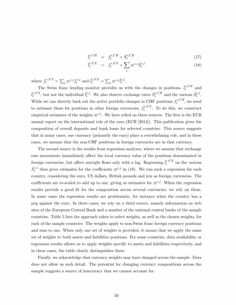
lc,CHt = f c,CH

t + Sc,CHt (17)

lc,FXt = f c,FX

t +∑

j

c,jSc,jt (18)

where f c,FXt =

∑

j c,jf c,j

t and lc,FXt =

∑

j c,j lc,jt .

The Swiss franc lending monitor provides us with the changes in positions, lc,CHt and

lc,FXt , but not the individual lc,jt . We also observe exchange rates Sc,CH

t and the various Sc,jt .

While we can directly back out the active portfolio changes in CHF positions f c,CHt , we need

to estimate these for positions in other foreign currencies, f c,FXt . To do this, we construct

empirical estimates of the weights c,j. We have relied on three sources. The first is the ECB

annual report on the international role of the euro (ECB [2014]). This publication gives the

composition of overall deposits and bank loans for selected countries. This source suggests

that in many cases, one currency (primarily the euro) plays a overwhelming role, and in these

cases, we assume that the non-CHF positions in foreign currencies are in that currency.

The second source is the results from regression analyses, where we assume that exchange

rate movements immediately affect the local currency value of the positions denominated in

foreign currencies, but affect outright flows only with a lag. Regressing lc,FXt on the various

Sc,jt then gives estimates for the coefficients c,j in (18). We run such a regression for each

country, considering the euro, US dollars, British pounds and yen as foreign currencies. The

coefficients are re-scaled to add up to one, giving us estimates for c,j. When the regression

results provide a good fit for the composition across several currencies, we rely on them.

In some cases the regression results are problematic, for instance when the country has a

peg against the euro. In these cases, we rely on a third source, namely information on web

sites of the European Central Bank and a number of the national central banks of the sample

countries. Table 5 lists the approach taken to select weights, as well as the chosen weights, for

each of the sample countries. The weights apply to non-Swiss franc foreign currency positions

and sum to one. When only one set of weights is provided, it means that we apply the same

set of weights to both assets and liabilities positions. For some countries, data availability or

regression results allows us to apply weights specific to assets and liabilities respectively, and

in these cases, the table clearly distinguishes these.

Finally, we acknowledge that currency weights may have changed across the sample. Data

does not allow us such detail. The potential for changing currency compositions across the

sample suggests a source of inaccuracy that we cannot account for.

50

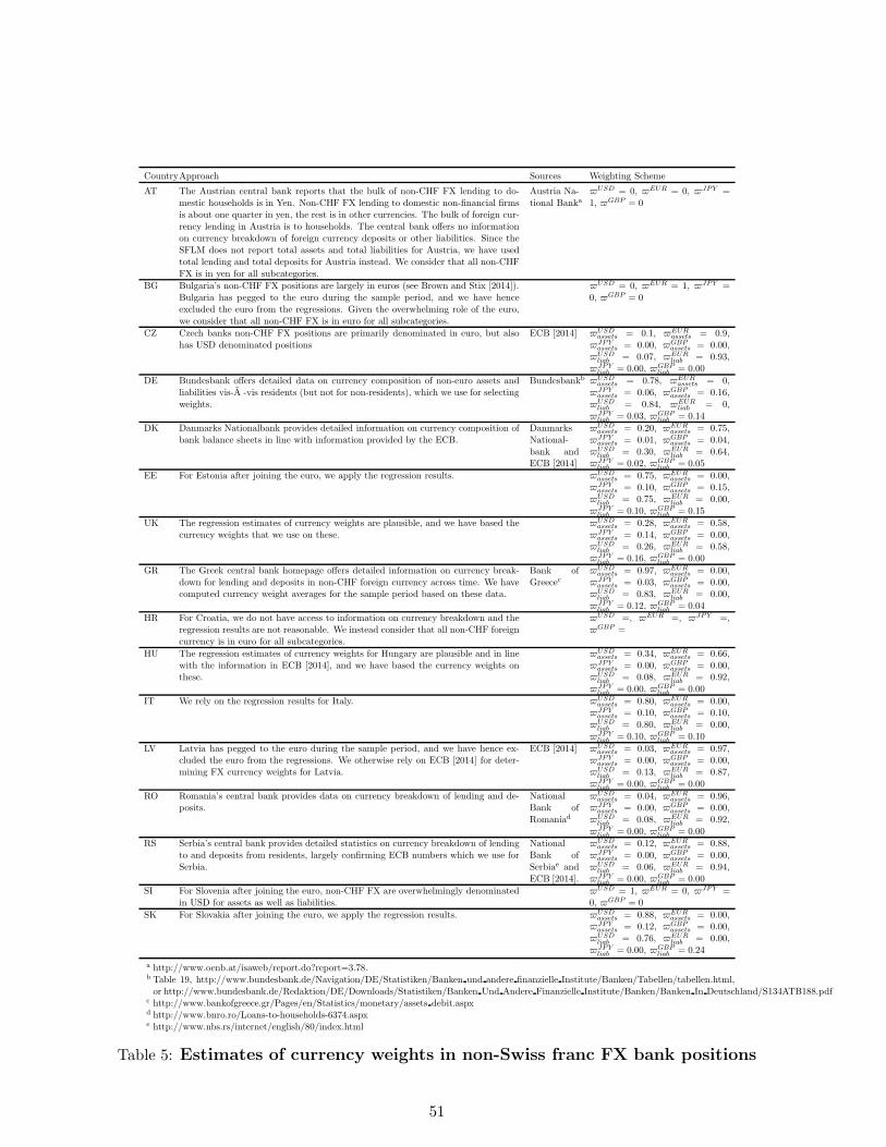
CountryApproach Sources Weighting Scheme

AT The Austrian central bank reports that the bulk of non-CHF FX lending to do-mestic households is in Yen. Non-CHF FX lending to domestic non-financial firmsis about one quarter in yen, the rest is in other currencies. The bulk of foreign cur-rency lending in Austria is to households. The central bank offers no informationon currency breakdown of foreign currency deposits or other liabilities. Since theSFLM does not report total assets and total liabilities for Austria, we have usedtotal lending and total deposits for Austria instead. We consider that all non-CHFFX is in yen for all subcategories.

Austria Na-tional Banka

USD = 0, EUR = 0, JPY =1, GBP = 0

BG Bulgaria’s non-CHF FX positions are largely in euros (see Brown and Stix [2014]).Bulgaria has pegged to the euro during the sample period, and we have henceexcluded the euro from the regressions. Given the overwhelming role of the euro,we consider that all non-CHF FX is in euro for all subcategories.

USD = 0, EUR = 1, JPY =0, GBP = 0

CZ Czech banks non-CHF FX positions are primarily denominated in euro, but alsohas USD denominated positions

ECB [2014] USDassets = 0.1, EUR

assets = 0.9,JPY

assets = 0.00, GBPassets = 0.00,

USDliab = 0.07, EUR

liab = 0.93,JPY

liab = 0.00, GBPliab = 0.00

DE Bundesbank offers detailed data on currency composition of non-euro assets andliabilities vis-A -vis residents (but not for non-residents), which we use for selectingweights.

Bundesbankb USDassets = 0.78, EUR

assets = 0,JPY

assets = 0.06, GBPassets = 0.16,

USDliab = 0.84, EUR

liab = 0,JPY

liab = 0.03, GBPliab = 0.14

DK Danmarks Nationalbank provides detailed information on currency composition ofbank balance sheets in line with information provided by the ECB.

DanmarksNational-bank andECB [2014]

USDassets = 0.20, EUR

assets = 0.75,JPY

assets = 0.01, GBPassets = 0.04,

USDliab = 0.30, EUR

liab = 0.64,JPY

liab = 0.02, GBPliab = 0.05

EE For Estonia after joining the euro, we apply the regression results. USDassets = 0.75, EUR

assets = 0.00,JPY

assets = 0.10, GBPassets = 0.15,

USDliab = 0.75, EUR

liab = 0.00,JPY

liab = 0.10, GBPliab = 0.15

UK The regression estimates of currency weights are plausible, and we have based thecurrency weights that we use on these.

USDassets = 0.28, EUR

assets = 0.58,JPY

assets = 0.14, GBPassets = 0.00,

USDliab = 0.26, EUR

liab = 0.58,JPY

liab = 0.16, GBPliab = 0.00

GR The Greek central bank homepage offers detailed information on currency break-down for lending and deposits in non-CHF foreign currency across time. We havecomputed currency weight averages for the sample period based on these data.

Bank ofGreecec

USDassets = 0.97, EUR

assets = 0.00,JPY

assets = 0.03, GBPassets = 0.00,

USDliab = 0.83, EUR

liab = 0.00,JPY

liab = 0.12, GBPliab = 0.04

HR For Croatia, we do not have access to information on currency breakdown and theregression results are not reasonable. We instead consider that all non-CHF foreigncurrency is in euro for all subcategories.

USD =, EUR =, JPY =,GBP =

HU The regression estimates of currency weights for Hungary are plausible and in linewith the information in ECB [2014], and we have based the currency weights onthese.

USDassets = 0.34, EUR

assets = 0.66,JPY

assets = 0.00, GBPassets = 0.00,

USDliab = 0.08, EUR

liab = 0.92,JPY

liab = 0.00, GBPliab = 0.00

IT We rely on the regression results for Italy. USDassets = 0.80, EUR

assets = 0.00,JPY

assets = 0.10, GBPassets = 0.10,

USDliab = 0.80, EUR

liab = 0.00,JPY

liab = 0.10, GBPliab = 0.10

LV Latvia has pegged to the euro during the sample period, and we have hence ex-cluded the euro from the regressions. We otherwise rely on ECB [2014] for deter-mining FX currency weights for Latvia.

ECB [2014] USDassets = 0.03, EUR

assets = 0.97,JPY

assets = 0.00, GBPassets = 0.00,

USDliab = 0.13, EUR

liab = 0.87,JPY

liab = 0.00, GBPliab = 0.00

RO Romania’s central bank provides data on currency breakdown of lending and de-posits.

NationalBank ofRomaniad

USDassets = 0.04, EUR

assets = 0.96,JPY

assets = 0.00, GBPassets = 0.00,

USDliab = 0.08, EUR

liab = 0.92,JPY

liab = 0.00, GBPliab = 0.00

RS Serbia’s central bank provides detailed statistics on currency breakdown of lendingto and deposits from residents, largely confirming ECB numbers which we use forSerbia.

NationalBank ofSerbiae andECB [2014].

USDassets = 0.12, EUR

assets = 0.88,JPY

assets = 0.00, GBPassets = 0.00,

USDliab = 0.06, EUR

liab = 0.94,JPY

liab = 0.00, GBPliab = 0.00

SI For Slovenia after joining the euro, non-CHF FX are overwhelmingly denominatedin USD for assets as well as liabilities.

USD = 1, EUR = 0, JPY =0, GBP = 0

SK For Slovakia after joining the euro, we apply the regression results. USDassets = 0.88, EUR

assets = 0.00,JPY

assets = 0.12, GBPassets = 0.00,

USDliab = 0.76, EUR

liab = 0.00,JPY

liab = 0.00, GBPliab = 0.24

a http://www.oenb.at/isaweb/report.do?report=3.78.b Table 19, http://www.bundesbank.de/Navigation/DE/Statistiken/Banken und andere finanzielle Institute/Banken/Tabellen/tabellen.html,or http://www.bundesbank.de/Redaktion/DE/Downloads/Statistiken/Banken Und Andere Finanzielle Institute/Banken/Banken In Deutschland/S134ATB188.pdf

c http://www.bankofgreece.gr/Pages/en/Statistics/monetary/assets debit.aspxd http://www.bnro.ro/Loans-to-households-6374.aspxe http://www.nbs.rs/internet/english/80/index.html

Table 5: Estimates of currency weights in non-Swiss franc FX bank positions

51

D Appendix Figures

-8

-6

-4

-2

0

2

4

6

8

2007 2008 2009 2010 2011 2012 2013 2014 2015

(a) Austria

-8

-6

-4

-2

0

2

4

6

8

2007 2008 2009 2010 2011 2012 2013 2014 2015

(b) Bulgaria

-8

-6

-4

-2

0

2

4

6

8

2007 2008 2009 2010 2011 2012 2013 2014 2015

(c) Czech Republic

-8

-6

-4

-2

0

2

4

6

8

2007 2008 2009 2010 2011 2012 2013 2014 2015

(d) Germany

-8

-6

-4

-2

0

2

4

6

8

2007 2008 2009 2010 2011 2012 2013 2014 2015

(e) Estonia

-8

-6

-4

-2

0

2

4

6

8

2007 2008 2009 2010 2011 2012 2013 2014 2015

(f) Greece

Figure 6: Net foreign currency and domestic currency wholesale funding inflowsThe black line is quarterly valuation adjusted change in foreign currency interbank funding less foreign

currency interbank lending, divided by total bank assets. The gray line is quarterly domestic currency

foreign interbank funding less domestic currency foreign interbank lending, divided by total bank

assets. Valuation adjusted as in Krogstrup and Tille [2017a]. Source: The Swiss Franc Lending

Monitor, SNB

52

-8

-6

-4

-2

0

2

4

6

8

2007 2008 2009 2010 2011 2012 2013 2014 2015

(a) Croatia

-8

-6

-4

-2

0

2

4

6

8

2007 2008 2009 2010 2011 2012 2013 2014 2015

(b) Hungary

-8

-6

-4

-2

0

2

4

6

8

2007 2008 2009 2010 2011 2012 2013 2014 2015

(c) Italy

-8

-6

-4

-2

0

2

4

6

8

2007 2008 2009 2010 2011 2012 2013 2014 2015

(d) Romania

-8

-6

-4

-2

0

2

4

6

8

2007 2008 2009 2010 2011 2012 2013 2014 2015

(e) Serbia

-8

-6

-4

-2

0

2

4

6

8

2007 2008 2009 2010 2011 2012 2013 2014 2015

(f) Slovenia

Figure 7: Net total and foreign currency wholesale funding inflowsThe black line is quarterly valuation adjusted change in foreign currency interbank funding less foreign

currency interbank lending, divided by total bank assets. The gray line is quarterly domestic currency

foreign interbank funding less domestic currency foreign interbank lending, divided by total bank

assets. Valuation adjusted as in Krogstrup and Tille [2017a]. Source: The Swiss Franc Lending

Monitor, SNB

53

-8

-6

-4

-2

0

2

4

6

8

2007 2008 2009 2010 2011 2012 2013 2014 2015

(a) Slovakia

-8

-6

-4

-2

0

2

4

6

8

2007 2008 2009 2010 2011 2012 2013 2014 2015

(b) United Kingdom

-8

-6

-4

-2

0

2

4

6

8

2007 2008 2009 2010 2011 2012 2013 2014 2015

(c) Latvia

-8

-6

-4

-2

0

2

4

6

8

2007 2008 2009 2010 2011 2012 2013 2014 2015

(d) Denmark

Figure 8: Net total and foreign currency wholesale funding inflowsThe black line is quarterly valuation adjusted change in foreign currency interbank funding less foreign

currency interbank lending, divided by total bank assets. The gray line is quarterly domestic currency

foreign interbank funding less domestic currency foreign interbank lending, divided by total bank

assets. Valuation adjusted as in Krogstrup and Tille [2017a]. Source: The Swiss Franc Lending

Monitor, SNB

54

-.16

-.12

-.08

-.04

.00

.04

.08

.12

.16

2007 2008 2009 2010 2011 2012 2013 2014 2015

(a) Austria

-.16

-.12

-.08

-.04

.00

.04

.08

.12

.16

2007 2008 2009 2010 2011 2012 2013 2014 2015

(b) Bulgaria

-.16

-.12

-.08

-.04

.00

.04

.08

.12

.16

2007 2008 2009 2010 2011 2012 2013 2014 2015

(c) Czech Republic

-.16

-.12

-.08

-.04

.00

.04

.08

.12

.16

2007 2008 2009 2010 2011 2012 2013 2014 2015

(d) Germany

-.16

-.12

-.08

-.04

.00

.04

.08

.12

.16

2007 2008 2009 2010 2011 2012 2013 2014 2015

(e) Estonia

-.16

-.12

-.08

-.04

.00

.04

.08

.12

.16

2007 2008 2009 2010 2011 2012 2013 2014 2015

(f) Greece

Figure 9: Foreign currency mismatch.The black line is the difference between foreign currency assets and foreign currency liabilities as

a share of total bank assets. The gray line is foreign currency interbank cross border lending less

similarly defined funding, as a share of total bank assets. Source: The Swiss Franc Lending Monitor,

SNB.

55

-.16

-.12

-.08

-.04

.00

.04

.08

.12

.16

2007 2008 2009 2010 2011 2012 2013 2014 2015

(a) Croatia

-.16

-.12

-.08

-.04

.00

.04

.08

.12

.16

2007 2008 2009 2010 2011 2012 2013 2014 2015

(b) Hungary

-.16

-.12

-.08

-.04

.00

.04

.08

.12

.16

2007 2008 2009 2010 2011 2012 2013 2014 2015

(c) Italy

-.16

-.12

-.08

-.04

.00

.04

.08

.12

.16

2007 2008 2009 2010 2011 2012 2013 2014 2015

(d) Romania

-.16

-.12

-.08

-.04

.00

.04

.08

.12

.16

2007 2008 2009 2010 2011 2012 2013 2014 2015

(e) Serbia

-.16

-.12

-.08

-.04

.00

.04

.08

.12

.16

2007 2008 2009 2010 2011 2012 2013 2014 2015

(f) Slovenia

Figure 10: Foreign currency mismatch.The black line is the difference between foreign currency assets and foreign currency liabilities as

a share of total bank assets. The gray line is foreign currency interbank cross border lending less

similarly defined funding, as a share of total bank assets. Source: The Swiss Franc Lending Monitor,

SNB.

56

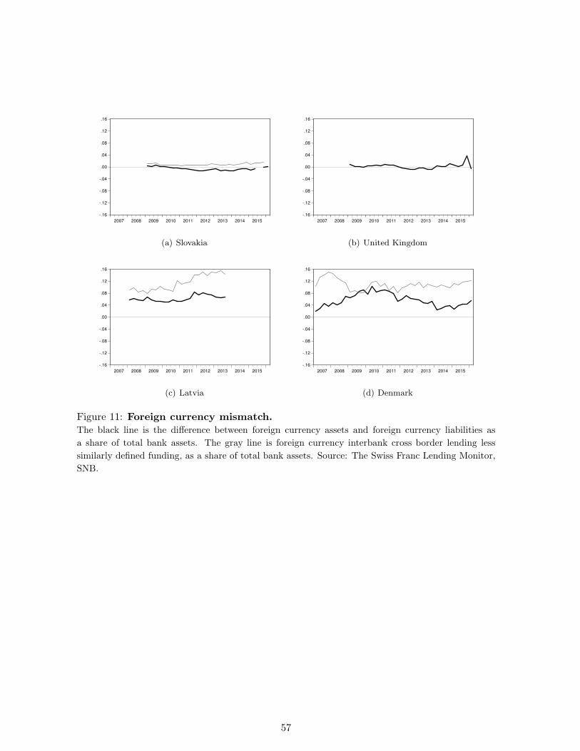
-.16

-.12

-.08

-.04

.00

.04

.08

.12

.16

2007 2008 2009 2010 2011 2012 2013 2014 2015

(a) Slovakia

-.16

-.12

-.08

-.04

.00

.04

.08

.12

.16

2007 2008 2009 2010 2011 2012 2013 2014 2015

(b) United Kingdom

-.16

-.12

-.08

-.04

.00

.04

.08

.12

.16

2007 2008 2009 2010 2011 2012 2013 2014 2015

(c) Latvia

-.16

-.12

-.08

-.04

.00

.04

.08

.12

.16

2007 2008 2009 2010 2011 2012 2013 2014 2015

(d) Denmark

Figure 11: Foreign currency mismatch.The black line is the difference between foreign currency assets and foreign currency liabilities as

a share of total bank assets. The gray line is foreign currency interbank cross border lending less

similarly defined funding, as a share of total bank assets. Source: The Swiss Franc Lending Monitor,

SNB.

57

E Appendix tables

58

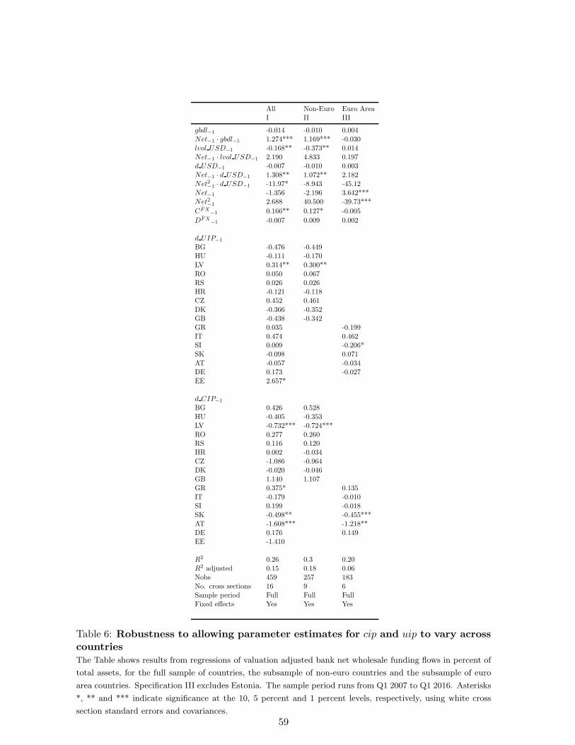
All Non-Euro Euro AreaI II III

gbdl−1 -0.014 -0.010 0.004

Net−1 · gbdl−1 1.274*** 1.169*** -0.030

lvol USD−1 -0.168** -0.373** 0.014

Net−1 · lvol USD

−1 2.190 4.833 0.197d USD

−1 -0.007 -0.010 0.003Net

−1 · d USD−1 1.308** 1.072** 2.182

Net2−1 · d USD

−1 -11.97* -8.943 -45.12Net

−1 -1.356 -2.196 3.642***Net2

−1 2.688 40.500 -39.73***¯CFX

−1 0.166** 0.127* -0.005¯DFX

−1 -0.007 0.009 0.002

d UIP−1

BG -0.476 -0.449HU -0.111 -0.170LV 0.314** 0.300**RO 0.050 0.067RS 0.026 0.026HR -0.121 -0.118CZ 0.452 0.461DK -0.366 -0.352GB -0.438 -0.342GR 0.035 -0.199IT 0.474 0.462SI 0.009 -0.206*SK -0.098 0.071AT -0.057 -0.034DE 0.173 -0.027EE 2.657*

d CIP−1

BG 0.426 0.528HU -0.405 -0.353LV -0.732*** -0.724***RO 0.277 0.260RS 0.116 0.120HR 0.002 -0.034CZ -1.086 -0.964DK -0.020 -0.046GB 1.140 1.107GR 0.375* 0.135IT -0.179 -0.010SI 0.199 -0.018SK -0.498** -0.455***AT -1.608*** -1.218**DE 0.176 0.149EE -1.410

R2 0.26 0.3 0.20R2 adjusted 0.15 0.18 0.06Nobs 459 257 183No. cross sections 16 9 6Sample period Full Full FullFixed effects Yes Yes Yes

Table 6: Robustness to allowing parameter estimates for cip and uip to vary acrosscountriesThe Table shows results from regressions of valuation adjusted bank net wholesale funding flows in percent of

total assets, for the full sample of countries, the subsample of non-euro countries and the subsample of euro

area countries. Specification III excludes Estonia. The sample period runs from Q1 2007 to Q1 2016. Asterisks

*, ** and *** indicate significance at the 10, 5 percent and 1 percent levels, respectively, using white cross

section standard errors and covariances.

59

All Non-Euro Euro AreaI II III

gbdl−1 -0.011 -0.027 0.012**

Net−1 · gbdl−1 1.356*** 1.435*** -0.280

lvol USD−1 -0.200** -0.290 -0.048

Net−1 · lvol USD

−1 1.133 2.224 0.428d USD

−1 -0.005 -0.017 0.011Net

−1 · d USD−1 1.410** 1.272** 0.862

Net2−1 · d USD

−1 -12.11* -9.377 1.817Net

−1 -3.948 -6.931* 6.192Net2

−1 0.909 28.901 -14.362¯CFX

−1 0.138* 0.116 -0.065¯DFX

−1 -0.020 -0.028 -0.009d UIP

−1 0.021 -0.006 -0.161**d CIP

−1 -0.094 -0.079 0.046Growth

−1 0.022 0.020 0.007Inflation

−1 0.057 0.060 0.029dUS TS

−1 -0.135** -0.350*** 0.051dUS RR

−1 0.047 0.098 -0.031d USREER

−1 -0.010 -0.013 -0.005DUSM0

−1 0.003 0.017 -0.001DUSSFFR

−1 0.360** 0.516* -0.001

R2 0.25 0.32 0.22R2 adjusted 0.19 0.23 0.08Nobs 421 238 166No. cross sections 16 9 6Sample period Full Full FullFixed effects Yes Yes Yes

Table 7: Robustness to inclusion of additional controlsThe Table shows results from regressions of valuation adjusted bank net wholesale funding flows in percent

of total assets, for the full sample of countries, the sub-sample of non-euro countries and the sub-sample of

euro area countries. Specification III excludes Estonia. The sample period runs from Q1 2007 to Q1 2016.

Asterisks *, ** and *** indicate significance at the 10, 5 percent and 1 percent levels, respectively, using white

cross section standard errors and covariances.

60

All Non-Euro Euro AreaI II III

gbdl−1 -0.016 -0.016 -0.011

Net−1 · gbdl−1 0.375 0.410* 0.166

lvol USD−1 -0.046 -0.005 -0.063

Net−1 · lvol USD

−1 1.416 1.211 10.07*d USD

−1 -0.005 -0.008 0.020Net

−1 · d USD−1 -0.234 -0.424 0.240

Net2−1

· d USD−1 1.294 4.155 -15.453

Net−1 -2.293 -6.901** 29.55*

Net2−1

38.243 68.43*** 61.748¯CFX

−1 0.033 -0.007 -0.177¯DFX

−1 -0.030 0.001 0.475d UIP

−1 -0.069** -0.028 -0.629***d CIP

−1 0.103** 0.041 0.371

R2 0.05 0.15 0.16R2 adjusted 0.00 0.08 0.07Nobs 467 265 183No. cross sections 16 9 6Sample period Full Full FullFixed effects Yes Yes Yes

Table 8: Regression for total cross border flows denominated in domestic currencyThe Table shows the results for regression with the alternative dependent variable that includes do-

mestic currency denominated cross border flows to foreign banks. Column III excludes Estonia from

the euro area sample. The sample runs from Q1 2007 to Q1 2016 and all regressions include country

fixed effects as well as the three explanatory variables. Asterisks *, ** and *** indicate significance

at the 10, 5 percent and 1 percent levels, respectively, using white cross section standard errors and

covariances.

61