Foreign Aid, Donor Fragmentation, and Economic Growth · Volume 9, Issue 1 2009 Article 33 Foreign...

Foreign Aid, Donor Fragmentation, and Economic Growth

Kurt Annen Department of Economics and Finance, University of Guelph

[email protected]

Stephen Kosempel Department of Economics and Finance, University of Guelph

[email protected]

Department of Economics and Finance University of Guelph

Discussion Paper 2009-14

The final publication of this article is available at www.degruyter.com DOI: http://dx.doi.org/10.2202/1935-1690.1863

The B.E. Journal of Macroeconomics

ContributionsVolume 9, Issue 1 2009 Article 33

Foreign Aid, Donor Fragmentation, andEconomic Growth

Kurt Annen∗ Stephen Kosempel†

∗University of Guelph, [email protected]†University of Guelph, [email protected]

Recommended CitationKurt Annen and Stephen Kosempel (2009) “Foreign Aid, Donor Fragmentation, and EconomicGrowth,” The B.E. Journal of Macroeconomics: Vol. 9: Iss. 1 (Contributions), Article 33.Available at: http://www.bepress.com/bejm/vol9/iss1/art33

Copyright c©2009 The Berkeley Electronic Press. All rights reserved.

Foreign Aid, Donor Fragmentation, andEconomic Growth∗

Kurt Annen and Stephen Kosempel

Abstract

This paper analyzes the impact of foreign aid on growth. It differs from the existing literaturein at least two important ways. First, we differentiate between foreign aid as technical assistanceand non-technical assistance, and demonstrate both theoretically and empirically that this distinc-tion is important. Second, we test the hypothesis that the effectiveness of aid depends on its levelof fragmentation. To preview our main results: non-technical assistance has no statistically sig-nificant impact on growth; but technical assistance has a positive and significant impact, except incountries where it is highly fragmented.

KEYWORDS: foreign aid, technical assistance, donor fragmentation, growth

∗We are grateful for helpful remarks and suggestions to Ryan Compton, Brian Ferguson, JoniadaMilla, Miana Plesca, Thanasis Stengos, Esteban Rossi-Hansberg, and two anonymous referees aswell as to seminar and conference participants at the University of Manitoba and Guelph, CanadianEconomic Association Meetings 2008 in Vancouver, and Small Open Economy in a GlobalizedWorld conference 2008 in Waterloo. The usual disclaimer applies.

1 IntroductionDoes foreign aid help countries grow? Are some forms of aid more effective thanothers? For many years economists and policymakers concerned with economicdevelopment have debated the answers to these important questions, but with littleresolution. The debate over the effectiveness of aid remains unresolved for at leasttwo reasons: First, in the background of this debate is a large empirical literature onthe impact of foreign aid on growth, in which the evidence in support of a positiverelationship between aid and growth is mixed. In this literature it is quite commonfor one paper to present a positive result, which is later overturned or qualified in asubsequent paper. Second, there exists a “micro-macro paradox” – projects fundedby foreign aid often report positive micro-level returns, but these have been difficultto detect at the macro-level. In fact, the results obtained from some of the morerecent papers in the empirical literature support the view that there is virtually noaggregate relationship between aid and growth across countries:

“. . . at best there appears to be a small, positive, but insignificant, im-pact of aid on growth.” (Bourguignon and Sundberg, 2007)

“. . . we find little robust evidence of a positive (or negative) relationshipbetween aid inflows into a country and its economic growth. We findvirtually no evidence that aid works better in better policy or institu-tional or geographical environments, or that certain kinds of aid workbetter than others.” (Rajan and Subramanian, 2008)

This paper argues that it is premature to draw strong policy conclusions on thebasis of the current empirical literature for at least two reasons. First, we differen-tiate between foreign aid as technical assistance (TA) and non-technical assistance(NTA), and demonstrate both theoretically and empirically that this distinction isimportant. Second, we believe that there are scale economies associated with theprovision of TA, and therefore its effectiveness may depend on how fragmentedit is. In our empirical work we show that there is a strong interaction effect be-tween donor fragmentation and TA, suggesting that the effectiveness of TA falls asfragmentation increases.

Within the context of a standard neo-classical growth model, we demonstratethat the effectiveness of aid depends on its type. TA is modeled as a knowledgetransfer that is intended to improve productive capabilities in the recipient country,whereas NTA is treated as an income transfer that adds to available resources forconsumption and investment.1 The theory says that TA, which affects productivity,

1Both types represent a substantial share of total aid. For example, in 2005 TA accounted for52% of total current and actual transfers for the average recipient.

1

Annen and Kosempel: Foreign Aid, Donor Fragmentation, and Economic Growth

Published by The Berkeley Electronic Press, 2009

should affect growth; whereas NTA, which enters the resource constraint, shouldnot. In our empirical work we provide evidence in support of these predictions.In comparison, most of the current literature uses aid measures as an aggregate ofmany different forms of aid including emergency and food aid, and debt forgivenessof loans that were not originally intended for development projects (i.e. debtforgive-ness of non-Official Development Assistance (ODA) loans).2 These aid measuresare not specific enough. It is not surprising that such macro measures yield incon-clusive results. In addition, in all of the current literature it is assumed that onedollar of aid equals one dollar of additional financial resources. However, the dis-bursement of foreign aid is costly. If the technology used for aid disbursementsexhibits increasing returns to scale, then the effectiveness of a given amount of aiddepends on how fragmented this amount of aid is. This is particularly true for TA.Donor countries that provide TA run local offices in recipient countries, or hireNGOs to run them on their behalf. To run these offices involves fixed costs in theform of maintaining offices typically in the fancier part of the capitals of develop-ing countries, living expenses for foreign engineers and consultants, etc. This maysuggest that the effectiveness of TA increases with the scale of the operation. Theremay be an interaction effect between TA and donor fragmentation. In fact, it will bedemonstrated that foreign aid, when given in the form of technical assistance, has apositive and statistically significant impact on growth, except in countries where itis highly fragmented.3

The basic underlying framework for our theoretical analysis of the aid-growthrelationship is the neo-classical growth model of Ramsey (1928)-Cass (1965)- Koop-mans (1965). Following Mankiw, Romer, and Weil (1992), we extend the produc-tion side of the basic model to allow for the accumulation of both physical and hu-man capital. Since NTA involves a transfer of income, it enters the model throughthe resource constraint. In comparison, TA enters the model through the human cap-ital production function, and in this way the model’s treatment of TA correspondsclosely with the OECD’s definition of it. TA is recorded by the OECD under tech-nical cooperation, and is defined as follows: “Technical co-operation is defined asactivities whose primary purpose is to augment the level of knowledge, skills, tech-

2Two exceptions are Clemens, Radelet, and Bhavnani (2004) and Minoiu and Reddy (2009).They observe that disaggregating aid measures is key for a better understanding of the impact of aidon growth.

3When calculating the fragmentation index, we follow Knack and Rahman (2007). Donor frag-mentation has increased substantially between 1970 and 2005, namely from 40% to 62%. In 2005,countries like Vietnam (86%), Nicaragua (86%), Gambia (85%), and Bangladesh (82%) had thehighest levels of donor fragmentation; whereas countries like Comoros (7.3%) and Solomon Is-lands (7.7%) had the lowest levels of fragmentation, with France and Australia as the major donorsrespectively.

2

The B.E. Journal of Macroeconomics, Vol. 9 [2009], Iss. 1 (Contributions), Art. 33

http://www.bepress.com/bejm/vol9/iss1/art33

nical know-how or productive aptitudes of the population of developing countries,i.e., increasing their stock of human intellectual capital, or their capacity for moreeffective use of their existing factor endowment.” Technical assistance is intendedto fill skills and knowledge gaps in developing countries. TA comes in two forms: Itis either linked to other aid projects, providing the technical component and know-how for these aid projects, or TA constitutes free-standing initiatives focusing ontraining and skills transfer (Riddell, 2007, p. 203). The distinction between TA andNTA matters. In the model, an increase in TA promotes income growth because itaffects productivity no matter whether the change in TA is perceived as being per-manent or temporary. In contrast, the model predicts that NTA is consumed entirelyif the change is perceived as being permanent. In this case, NTA does not promoteincome growth.

The papers that most closely resemble the theoretical component of this pa-per are Chatterjee, G., and Turnovsky (2003), Dalgaard, Hansen, and Tarp (2004),Hodler (2007), Chatterjee, Giuliano, and Ilker (2007), Chatterjee and Turnovsky(2007) and Agenor, Bayraktar, and Aynaoui (2008). The main feature that distin-guishes these earlier papers from ours is that they only consider income transfers,whereas we also consider the transfer of knowledge. In several of the papers men-tioned above, aid funds were allowed to be used to finance public infrastructure,and therefore - like TA - these funds may also have a productivity enhancing effect.However, unlike other forms of aid, one advantage of TA is that it is not fungible.4

The aid literature claims that fungibility may render most aid distinctions meaning-less.5 However, TA is to our knowledge mainly disbursed by the donor countriesthemselves or by NGOs working for donor countries. Thus, the view that aid is inthe form of a check that the government of a recipient country can spend at its owndiscretion does not apply to TA.6

In our empirical work we estimate the impact of technical- and non-technicalassistance on economic growth using the GMM system estimator developed byArellano and Bond (1991) and Blundell and Bond (1998). One of the advantagesof this estimator is that we do not need to deal with country specific effects such asinstitutional and cultural variables that are difficult to measure.7 We include policymeasures that control for a changing policy environment across time. This paperfinds, first, a strong interaction effect between TA pc and donor fragmentation. The

4Aid funds that are intended to help finance specific activities often merely substitute for spend-ing that recipient governments would have undertaken anyway.

5see Devarajan and Swaroop (1998).6TA is a form of tied aid as opposed to un-tied aid. See Amegashie, Quattara, and Strobl (2007)

for an economic model explaining why donor countries may use tied- as opposed to un-tied aid.7See Glaeser, La Porta, Lopez-de Silanes, and Shleifer (2004) for a critical discussion of the

institutional variables typically used in the literature.

3



partial impact of TA pc decreases as donor fragmentation increases. We obtain thisfinding no matter the time frame considered. Our result is also robust to the exactspecification of the empirical model and the normalization of aid used. For ourmain result we use the System GMM estimator, but we obtain a similar result forthe time horizon between 1970 and 2004 using IV estimation with an instrumenta-tion strategy similar to the one used in Rajan and Subramanian (2008). Second, theestimates suggest that tripling TA pc for the country receiving an average amount ofTA pc would increase its income growth rate by about 3 percentage points if donorfragmentation is zero.8 However, for the country with an average fragmentationlevel, we find no significant positive impact of TA pc on income growth at the fivepercent level.9 Our result for donor fragmentation suggests that donor fragmen-tation produces inefficiencies that greatly reduce the effectiveness of TA. From apolicy perspective, this paper provides evidence that the coordination of aid amongdonors is critical.

The papers most closely related to the empirical component of this paper areMinoiu and Reddy (2009) and Clemens, Radelet, and Bhavnani (2004). Both pa-pers disaggregate the ODA measure into different forms of aid. Minoiu and Reddy(2009) focus on aid which is developmental and non-developmental. They refer toaid that was given for geopolitical reason as non-developmental while the remain-ing aid is called developmental. They use an aid allocation regression to obtain theirmeasures. Using similar estimation techniques than here, they show that develop-mental aid has a significant positive impact on growth in the long run. Clemens,Radelet, and Bhavnani (2004) divide aid into three categories: humanitarian, long-run impact, and short-run impact aid. They find a strong positive causal relationshipbetween short-impact aid and growth. These two papers suggest that disaggregat-ing aid measures is a promising way of getting a better understanding of aid ongrowth. Our paper follows these approaches by distinguishing between aid in formof technical assistance and non-technical assistance. However, unlike these earlierpapers, we also study the impact of donor fragmentation on aid effectiveness. Ourwork on donor fragmentation is related to a recent paper by Knack and Rahman(2007). They show that donor fragmentation is inversely related to bureaucraticquality of recipient countries. However, they do not link donor fragmentation to aideffectiveness.

The rest of the paper is organized as follows. Section 2 outlines the theoreticalmodel. Section 3 presents the empirical results. Section 4 evaluates the robustnessof the results. Finally, Section 5 concludes.

8To give 0.7 percent of their GNP as official development assistance is often discussed as a targetin policy circles, which means that aid would more than triplicate from 0.2 percent of GNP in 2002.

9But note that in a specification without donor fragmentation, the coefficient for TA pc is positiveand significant at the ten percent level.

4



2 Aid and Growth: Theoretical AnalysisThis section provides the theoretical rationale for disaggregating aid according towhether it takes the form of TA or NTA.10 The basic framework is due to Ramsey(1928), Cass (1965) and Koopmans (1965). However, following Mankiw, Romer,and Weil (1992), we extend the production side of the basic model to allow forthe accumulation of both physical and human capital. The convention throughoutthe paper is to use upper case letters to denote per capita variables, lower caseletters to denote variables that have been transformed into effective labor units, astar superscript (*) to denote a long-run or steady-state value, and a dot over avariable to denote a time derivative.

We consider a closed economy populated by a large number of infinitely livedand identical households. The size of each household grows at rate n. The repre-sentative household seeks to maximize lifetime utility by choosing an optimal pathfor consumption and investment. The lifetime utility function is given by

U =

∫ ∞

t=0

u[C(t)]e−(ρ−n)tdt, (1)

where C(t) denotes consumption per person, and ρ is the constant rate of timepreference. The instantaneous utility function is assumed to take the constant in-tertemporal elasticity of substitution form

u[C(t)] =C(t)1−θ − 1

1− θ, (2)

where θ > 0 is the reciprocal of the elasticity of intertemporal substitution.In a given recipient country of foreign aid, each household-producer has access

to a Cobb-Douglas constant returns to scale production technology

Y (t) = X(t)1−α−βK(t)αH(t)β, (3)X(t) = X(0)egt. (4)

Here, Y (t) denotes GDP per person, K(t) and H(t) are the levels of physical andhuman capital per person, X(t) is the level of labor augmenting technology, and g isthe constant rate of technological change. Following most of the empirical growthliterature, it is assumed that the value of g is the same for all countries. However,countries may differ with respect to their initial productivity level, X(0).

10Easterly (2003) observes the lack of theoretical models on the aid growth relationship whichhelp to pin down the specification needed for empirical analysis.

5



The country receives aid in the form of technical and non-technical assistance.Non-technical aid affects the resource constraint, which is given by

Y (t) + NTA(t) = C(t) + IK(t) + IH(t), (5)

where NTA(t) denotes non-technical assistance per capita; and IK(t) and IH(t)denote investment in physical and human capital respectively. In contrast, technicalassistance is assumed to affect the productivity of human capital production, be-cause it is a transfer of knowledge. The laws of motion for capital are then givenby

K(t) = IK(t)− (δ + n)K(t), (6)H(t) = σ[TA(t)/X(t)]× IH(t)− (δ + n)H(t), (7)

where δ denotes the rate of capital depreciation, σ is a function that describesproductivity in human capital production, and TA(t) is technical assistance percapita. A specific functional form for σ will not be required. We, however, assume:∂σ/∂TA > 0, ∂2σ/(∂TA · ∂X) < 0, and σ(0) = 1. These assumptions implythat TA has a positive effect on the productivity of human capital production, andtherefore it enters into the model in a way that corresponds closely to the OECDdefinition of technical co-operation, that is, as activities whose primary purpose isto augment the level of knowledge, skills, technical know-how, or productive ap-titudes of the population of the recipient countries. Furthermore, our assumptionsimply that TA is not an essential input into human capital production, and that TAwill be more effective in countries with relatively low levels of the labor augment-ing technology. In other words, TA will be more effective when given to countriesthat are farther from the world technology frontier.11

Finally, to complete the model, aid payments are assumed to grow in proportionto the income in donor countries. As indicated above, all countries are assumed tohave a common long-run growth rate, and therefore:

NTA(t) = NTA(0)egt. (8)TA(t) = TA(0)egt. (9)

The optimality conditions with respect to the representative household’s choicesof C, IK and IH are

C(t)−θe−(ρ−n)t = ψ(t), (10)−ψ(t)[αY (t)/K(t)− δ − n] = ψ(t), (11)

−ψ(t)[βσ(t)Y (t)/H(t)− δ − n] = ψ(t), (12)11In Mankiw, Romer, and Weil (1992) the production functions for physical and human capital

are identical; whereas here they will differ if a country is a recipient of TA, because TA lowers thecost of acquiring an additional unit of human capital.

6



where ψ(t) is the present-value shadow price of income. These conditions implythat the optimal solution to the representative household’s maximization problemrequires that households set their investment levels to equalize rates of return be-tween the two types of capital. This produces the following ratio of human-to-physical capital:

H(t) =

[βσ(t)

α

]K(t). (13)

In turn, this result is used to substitute out for H , and reduce the model to a systemof two differential equations and two unknowns (C and K). The maximization ofthe representative household’s lifetime utility implies that the growth rate of con-sumption per effective unit of labor (c ≡ C/X) and capital per effective unit oflabor (k ≡ K/X) at each point in time are given by

c(t)

c(t)=

1

θ

(αAk(t)α+β−1 − δ − ρ− θg

), (14)

(1 + β/α)k(t) = Ak(t)α+β + nta− (δ + n + g)(1 + β/α)k(t)− c(t),(15)

where

A ≡[β

ασ(ta)

]β

. (16)

Here nta and ta are constants and denote the levels of non-technical and technicalaid per effective unit of labor.

A well known feature of the basic Ramsey-Cass-Koopmans model is that itexhibits saddle path stability. Although the basic structure has been augmented toincorporate foreign aid, the equilibrium is still a saddle point.12 The phase diagramfor the model is displayed in Figure 1. Expressions for the c = 0 and k = 0 loci aregiven by:

c = 0 ⇒ k∗ =

[αA

δ + ρ + θg

] 11−α−β

, (18)

k = 0 ⇒ c∗ = A(k∗)α+β + nta− (δ + n + g)(1 + β/α)k∗. (19)

12The saddle path property can be verified by log-linerizing the dynamic system for c and karound the steady state and showing that the determinant of the characteristic matrix is negative. Aclosed form solution exists for the log-linearized version. The solution for the growth rate of percapita output over an interval from some initial time 0 to a future time T ≥ 0 is given by

ln Y (T )− ln Y (0)T

= g +(1− e−λT )

T[ln X(0) + ln y∗ − ln Y (0)], (17)

where λ is the speed of convergence. This is the base equation for the empirical part of this paper.

7



Since the general properties of the model are well known, our discussion focusesonly on how an economy will respond to a change in its levels of foreign aid. Sincethe two different forms of aid enter differently into the model, the comparativestatics properties are distinct.

First, consider the effects of an increase in the level of technical assistance.Suppose that the economy is in the long-run equilibrium (at point E in panel (a) inFigure 1), and there is an unexpected, permanent increase in technical assistance:ta → ta′. The increase in ta lowers the cost of acquiring an additional unit ofhuman capital, and therefore the stock of human capital rises. In turn, this increasesthe marginal product of physical capital, which shifts the k = 0 locus up and thec = 0 locus to the right.13 The economy jumps to a new saddle path (SP → SP ′),and proceeds to a new long-run equilibrium at E ′, which has more capital andhigher output.14 In comparison, if the change was perceived as being temporary,then the long-run equilibrium would remain at E. However, the influx of ta wouldstill temporarily lower the cost of acquiring human capital. As such, an economythat was initially at E, would over accumulate capital relative to the long-run level,and income growth would be temporarily high. However, if the terminal date wasknown, then when the aid level returned to normal, the economy would find itselfback on the saddle path SP to the initial equilibrium.15

Next, consider the effects of an increase in the level of non-technical assistance.Once again suppose that there is an unexpected permanent increase in non-technicalassistance when the economy is in the long-run equilibrium (at point E in panel (b)in Figure 1): nta → nta′. The increase in nta raises the amount of resourcesavailable for consumption and investment, and therefore shifts the k = 0 locus(parallel) upwards. However, unlike technical assistance, nta does not have a directeffect on productivity or the rate of return to capital, and therefore the c = 0 locusis unaffected. The economy jumps to a new saddle path, with a higher level ofconsumption. Notice that the economy moves instantaneously to its new long-runequilibrium, and this is because the long-run level of capital has not changed. Thesavings rate applied to additional nta is zero. Instead of saving out of new aidmoney, households obtain their desired consumption profile by consuming it all

13This can be seen in the expressions above since the productivity parameter, A, depends posi-tively on ta.

14The initial effect on consumption is ambiguous, but it rises in the long-run.15A similar analysis applies to an economy in transition. In the case of a unexpected, permanent

increase in ta, the additional aid pushes the economy farther from the steady-state position, andtherefore leads to faster growth in income. For the temporary case, the economy will operate off thesaddle path during the periods in which the additional aid is received. Investment will rise duringperiods in which additional ta is available, and this is because the economy will take advantage ofthe relatively low cost of acquiring human capital.

8



(a) An increase in technical assistance

(b) An increase in non-technical assistance

0 k

)0( ! k

0 c )0( ! c

SP

PS !

k

c

E

E !

0 k

)0( ! k

0 c

SP

PS !

k

c

E

E !

nta

ant !

*k

*k

)( *!k

nta

Figure 1: Phase Diagram

9



each period. In comparison, if the change was perceived as being temporary, thenthe long-run equilibrium would remain at E. However, the economy will initiallyfollow a path away from E, and therefore it will over accumulate capital relativeto the steady-state level. If the terminal date is known with certainty, then theeconomy must find itself back on the saddle path exactly when the aid level returnsto normal. The intuition for this result is that in order to smooth their consumptionprofile, households will optimally save (or invest) some of the additional nta. Theadditional savings will be used to support relatively high consumption levels whenaid payments revert back to normal levels, and therefore consumption levels willfollow a smooth transition. The more temporary the change is perceived, the largerwill be the effect on the savings rate, the capital stock, and output.

Note that for both types of aid the responses follow standard macro-intuition.For TA, responses are identical to models with investment specific technical change.In those models, an investment specific technology shock affects the relative priceof physical capital, whereas in our model a change in TA affects the relative priceof human capital. For NTA, responses follow directly from the permanent incomehypothesis.

In summary, the model reveals that foreign aid can have a positive effect ongrowth of income per capita in poor countries. This prediction of the model isnecessarily true for technical assistance, but for non-technical assistance the resultdepends on whether the change is viewed as being temporary or permanent. Inaddition, given our modeling assumptions, we expect to find a more significanteffect of foreign aid on income growth at shorter time horizons. Only a permanentincrease in technical assistance is expected to have a long-term effect on capital andincome.

Despite what the model predicts for TA, Riddell (2007) refers to “a growingconsensus – not least among many leading official donors – that TA, as tradition-ally given, has largely been a failure.” However, Riddell also notes that surprisinglyenough there is little evidence of studies that have assessed the results and impactof TA. The assessment that TA has mainly been a failure stems from two kinds ofobservations among others: First, the costs of providing TA have always been veryhigh. Riddell reports that for example the yearly costs of employing a foreign con-sultant amounted to about $150,000 in the early 80s. Today, this amount is probablythe double. A second problem associated with TA is duplication of activities whichhas arisen because donors failed to consult with each other. For example, Riddell(2007, p. 205) claims that “it was not uncommon in the past, and still not unknowntoday, for long-term consultants, working in a ministry to discover other consul-tants, located even along the same corridor, funded by other donors to do workoverlapping with their own.” In the next section we will provide empirical evidencein support of a positive relationship between TA and income growth, and we will

10



address the possibility of overlap by including donor fragmentation of TA into ourregression analysis.

3 Aid and Growth: Empirical AnalysisThe model developed previously distinguishes between technical assistance andnon-technical assistance and shows that TA enhances economic growth at least inthe short run no matter whether this form of aid is perceived as being permanent ortemporary. In contrast, NTA does not increase income growth rates when perceivedas being permanent.

In order to test these predictions, we separate between these two forms of aidand estimate the following model using a sample of 105 countries:16

yi,t − yi,t−1

T= b0 + b1yi,t−1 + b2TAi,t + b3NTAi,t + b4X

′i,t (20)

+ b5Fi,t + b6Fi,t × TAi,t + φi + ϕt + εi,t,

where the subscript i indexes countries, t indexes periods, and T measures periodlength. For our main result we use data between 1970 and 2004 and divide thislength into eight 4-year and one 3-year period indexed by t ∈ {1, . . . , 9}. We use4-year periods because they have been used elsewhere (for example, Burnside andDollar (2000)). We use period averages to estimate the impact of foreign aid ongrowth. This procedure is done to account for business cycle movements.17

The dependent variable is the average annual growth rate of real per capita GDPduring period t. yi,t−1 is the logarithm of real per capita GDP in the last year ofperiod t − 1. TAit and NTAi,t are the average per capita levels during period tfor technical and non-technical assistance respectively. The aid data is from theOECD. TA is measured using the data series “technical cooperation.” For NTA wefocus on current and actual transfers, thereby following Roodman (2006). Weexclude all debt forgiveness grants and capitalized interest, none of which involvesactual movement of money.18 In addition, we exclude food and emergency aidfrom our measure since we believe that these forms of aid are not directly intended

16A list of the countries in the sample is provided in Table 7 in the Appendix. We include allcountries in our sample for which data is available.

17Note, however, that in Table 4 we present results when estimating (20) with varying definitionsof period length.

18Debt forgiveness would not affect any economic decisions if it was anticipated or if it was givenbecause the recipient is unable to service the debt.

11



for “development.” Subtracting TA from this measure then yields our measure forNTA.19 Both of our aid measures, TA and NTA, are PPP adjusted.

The vector X i,t is a vector of control variables that affect the steady state ofcountry i. Our strategy for selecting the appropriate controls is to adopt a spec-ification that is close to the one typically used in the aid effectiveness literature(e.g. Burnside and Dollar, 2000; Rajan and Subramanian, 2008). In particular, weinclude policy variables such as openness, M2/GDP, inflation, and budget balancedivided by GDP. We also include life expectancy and the average number of revolu-tions in a given period defined as any forced attempted or succeeded change in thetop of the government. Data sources are explained in Table 8 in the Appendix. Incontrast to the typical aid effectiveness literature, we also include a control for theinvestment rate. We have theoretical reasons to do so because the investment rateis an important control for the steady state of an economy. In Column (4) in Table3, however, we report results without the investment rate and we show that similarresults are obtained.

The variable Fi,t measures the average donor fragmentation of recipient countryi in period t. The fragmentation index is constructed by calculating a Herfindahlindex of donor concentration, which ranges from 0 to 1. This index is then sub-tracted from 1 and multiplied by 100. The value of donor fragmentation of zeroindicates completely unfragmented aid (i.e. one donor in a given country). Thefragmentation measure increases in the number of donors or with equality of aidshares. We argued in the introduction that if the technology for the disbursement ofTA exhibits increasing returns to scale, then less fragmented TA will have a largerimpact on growth rates than more fragmented TA. Furthermore, we indicated thatdonor duplication is a well known problem associated with TA (Riddell, 2007).We believe that this argument does not apply to foreign aid that is fungible andaffects the resource constraint of a country. For example, we do not expect the ef-fectiveness of NTA to depend on donor fragmentation. In order to test the impactof donor fragmentation on aid effectiveness, we include an interaction term of TAand donor fragmentation in our main specification. In Table 2 we report estimationresults when we also include an interaction term for NTA. The evidence reportedthere seems to support our claim that there is no interaction effect between donorfragmentation and NTA.

In (20), the partial impact of technical aid on growth equals b2 + b6 × F . Inaddition, the standard error of interest now is given by

σ ∂y∂TA

=

√var(b2) + Fvar(b6) + 2F cov(b2, b6). (21)

19Our aid measure NTA is derived from aid data reported by the OECD as follows: NTA=Total Grants-Debt Forgiveness Grants+ODA loans extended-Reorganized Debt-Emergency Aid-Development Food Aid-Technical Cooperation.

12



It is important to point out that the standard error now depends on the level of donorfragmentation, F . In particular, note that in case the estimates of b2 and b6 arenot statistically significant separately, they may nevertheless be significant jointly,since cov(b2, b6) can be negative.20 We hypothesize that b6 is negative so that theeffectiveness of aid decreases as donor fragmentation increases.

Finally φi and ϕt are country and time fixed effects. We use a country fixedeffect to properly control for unobserved time invariant variables that may be corre-lated with some of the independent variables. In particular, we do not need to con-trol for institutions, where only imperfect measures are available. Glaeser, La Porta,Lopez-de Silanes, and Shleifer (2004) provides a discussion of the institutionalmeasures used in the growth literature which highlights their limitations. By us-ing fixed effects, we avoid these limitations.21 Furthermore, fixed effects will alsocontrol for other permanent factors such as culture and initial level of technology.

Using a fixed effect estimator (FE) for equation (20), however, raises economet-ric issues. First, a fixed effect estimator yields consistent estimates if the so called“strict exogeneity” assumption holds. This assumption states that ei,t is not corre-lated with any other future, current, and past right-hand side variable in (20). Ina model with a lagged depended variable, the strict exogeneity assumption is nec-essarily violated (Woolbridge, 2002, p. 255). Thus, estimates using a fixed-effectestimator in this setting are biased. Monte Carlo simulations, however, show thatthe bias on the lagged dependent variable can be significant, while it tends to beminor for other right-hand side variables (Judson and Owen, 1996). This wouldbe true for foreign aid. There are estimators that are able to address the problem ofunobserved country fixed effects which do not require the strict exogeneity assump-tion. Building on Arellano and Bond (1991), Blundell and Bond (1998) developeda system estimator (GMM(sys)) that allows ei,t to be correlated with future valuesof the other right-hand side variables in (20) (but not with current and past val-ues) which is consistent with the generalized method-of-moments (GMM).22 Thisestimator uses lagged level variables as instruments for differences and lagged dif-ferences as instruments for level variables. Note that this instrumentation strategycan be implemented for any right hand side variable that one suspects to be en-

20Most of the critical discussion of the policy interaction term in Burnside and Dollar (2000) fo-cusses on the significance of the interaction term itself (see for example Easterly (2003) and Easterly,Levine, and Roodman (2004)). We believe this is misleading. For an assessment of aid effectiveness,one needs to focus on the point estimates and standard errors pointed out above. Brambor, Clark,and Golder (2006) provide a useful discussion of how to correctly interpret interaction terms.

21Note also that data on institutions is often available for a limited set of (developing) countriesand typically the data does not got far back.

22We use xtabond2 in Stata for our regressions. For a detailed description and for advice on howto use this command see Roodman (2009).

13



dogenous. For example, if foreign aid is given because of the “need” of a recipientcountry as its economy is under-performing, then treating aid as exogenous intro-duces a downward bias. For this reason we treat our aid variables as endogenousvariables where lagged level variables serve as an instrument for first differencesand lagged differences serve as an instrument for level variables. Note that in theresults reported we use only one lag, since using more lags can easily lead to weakinstrument problems.23

Column (4) in Table 1 reports our main result. Table 1 also includes ordinaryleast square (OLS), fixed-effect (FE), and GMM difference results for comparisonreasons. Since system GMM corrects for the bias introduced because of the inclu-sion of initial GDP per capita as a lagged dependent variable, the expectation is thatthe coefficient for initial GDP per capita is somewhere between the coefficient esti-mated using OLS and FE. This prediction is confirmed in Table 1. In addition, thepoint estimates on TA increase when comparing OLS and FE results with the GMMdifference and GMM system results. Difference and system GMM uses lagged aidvalues as instruments to address potential problems of endogeneity. Again, this re-sult is expected since treating aid as exogenous likely introduces a downward bias.In the following tables, we use system GMM for all estimations.

The results shown in Column (4) of Table 1 show a strong positive impact ofTA on income growth. The result suggest that increasing TA pc by 10 dollars willincrease the growth rate by 0.6 percentage points if donor fragmentation is zero.Note that in the sample, average TA pc is equal to about $30. To give 0.7 percentof GNP as official development assistance is often discussed as a reasonable targetamong policy makers. Reaching this target means that aid would more than tripli-cate from 0.2 percent of GNP in 2002. Accordingly, increasing TA by 50 dollarswill increase growth rates by about 3 percentage points if donor fragmentation iszero. The impact of TA pc on growth, however, declines as donor fragmentationincreases. For the typical developing country, donor fragmentation is quite high. Inour sample, the average donor fragmentation index for TA equals 65%.

The coefficient for the interaction term between donor fragmentation and TA issignificant and negative as expected. For example, with a donor fragmentation in-dex of 50%, a 50 dollar increase in per capita TA increases the growth rate by only0.75 percentage points as compared to the 3 percentage points if donor fragmenta-tion is zero. Furthermore, for the country with an average donor fragmentation, thepartial impact of TA pc on income growth is zero. Thus, our results suggest a stronginteraction effect between aid effectiveness and donor fragmentation. Using (21),

23We, hereby, follow Roodman (2009), who cautions from using too many instruments. Note,however, that increasing the number of lags does not affect our result. We obtain similar results nomatter the exact lag structure we use.

14



Table 1: Foreign Aid and Growth: Main Result

(1) (2) (3) (4)

Estimation method OLS FE GMM (diff) GMM (sys)

Initial GDP pc -1.51∗∗∗ -6.55∗∗∗ -12.0∗∗∗ -3.86∗∗∗(0.30) (0.94) (1.83) (0.98)

Investment/GDP 1.21∗∗∗ 1.07 -2.22 1.98∗(0.32) (0.82) (1.55) (1.12)

Openness 0.011∗∗∗ 0.013 0.043∗∗ 0.030∗(0.0038) (0.0094) (0.017) (0.017)

M2/GDP -0.035∗∗∗ -0.035∗∗∗ -0.074∗∗∗ -0.096∗∗∗(0.013) (0.0075) (0.0085) (0.017)

Inflation -0.0014∗∗∗ -0.0012∗∗∗ -0.0010∗∗∗ -0.0011∗∗(0.00042) (0.00022) (0.00024) (0.00047)

Budget balance/GDP 0.0051 0.0089 0.0012 -0.0018(0.0058) (0.0085) (0.010) (0.0099)

Revolutions -0.63∗∗ -0.82∗∗ -0.84∗∗ -0.78∗∗(0.25) (0.36) (0.34) (0.38)

Life expectancy 0.12∗∗∗ 0.050 0.11 0.24∗∗∗(0.029) (0.064) (0.11) (0.083)

TA pc 0.017 0.049∗∗∗ 0.077∗∗∗ 0.060∗∗∗(0.012) (0.013) (0.019) (0.017)

TA pc × frag. -0.00024 -0.00062∗∗ -0.00057 -0.00090∗∗∗(0.00020) (0.00026) (0.00047) (0.00030)

NTA pc 0.0020 -0.00073 -0.0011 0.0018(0.0025) (0.0035) (0.0045) (0.0042)

Donor Fragmentation 0.0086 0.00057 0.034 0.026(0.013) (0.023) (0.023) (0.023)

N 621 621 621 621Hansen over-id test 0.206 0.944AB(1) p-value 0.002 0AB(2) p-value 0.590 0.733Dependent Variable in all equations is average growth rates. Significance levels : ∗ : 10 ∗∗ :5% ∗ ∗ ∗ : 1%. Robust standard errors are in parenthesis. Constant term, time-, and country fixedeffects are not reported. AB(1) and AB(2) refers to the Arellano-Bond test for first and second orderzero autocorrelation respectively.

Figure 2 plots a 95% confidence interval for the partial impact of TA on growth forfragmentation levels between 0 and 100 based on the estimation results reported inColumn (4), Table 1. This figure confirms our hypothesis that the partial impact ofTA on growth decreases with an increasing level of fragmentation. For countrieswith a donor fragmentation below 51% we find a positive and statistically signif-icant impact of TA on growth at the 5% level. For levels of donor fragmentation

15



−.0

50

.05

.1

0 20 40 60 80 100Donor Fragmentation

Partial Impact of TA pc from Eq. (4) in Table 1

Figure 2: 95% Confidence Interval of Partial Impact of TA pc

exceeding 66%, b2 + b6 × F becomes negative but remains insignificant.In contrast to TA, the evidence suggests that there is no significant positive nor

negative impact of NTA on growth. The coefficient for NTA is not significant.There may be at least two reasons for this finding: First, the model introducedearlier suggests that if NTA is perceived as being permanent then the income growthrate does not change as a result of an influx of NTA.24 NTA is consumed insteadof being invested. Boone (1996) and more recently Chatterjee, Giuliano, and Ilker(2007) provide evidence that suggests that most of foreign aid is consumed ratherthan invested. The second reason for the finding may be that NTA is still a residualmeasure of aid. It may include some forms of aid that are not intended to fostereconomic development, and therefore a further disaggregation of this aid measureis needed in order to get a better understanding of the impact of NTA on growth.

Table 1 furthermore confirms other predictions of the neoclassical growth modelintroduced earlier. The countries in the sample exhibit conditional convergence(since the point estimates of initial GDP are negative), with an annual convergencerate of 4.2% for System GMM. This estimate is well within the rates observed inthe literature.25 We also find that the investment rate positively affects economic

24Recall that in the model the effect that a change in NTA has on income growth depends onwhether it is perceived as being permanent or temporay. Since we cannot observe from the data howchanges in aid levels are perceived, then pooling this shocks and estimating an average effect meanswe should find smaller effects for NTA than TA.

25See Barro and Sala-i Martin (2004) for a survey of the empirical growth literature.

16



growth. The estimate is significant in Column (4), although only at the 10% level.Openness has the expected sign and is significant at the 10% level. In contrast, bud-get balance has not the expected sign and is not significant. Finally, the remainingcontrol variables are revolutions and life expectancy, and they have the expectedsign and are significant.

4 Sensitivity AnalysisIn this section we analyze how sensitive the results presented in Column (4) ofTable 1 are to various changes to the estimation procedure. First, we analyze howour main result is affected by changing the specification of our regression model.Second, we analyze our empirical model when changing the definition of periodlength. In this subsection, we include a cross-sectional analysis looking at the timehorizon between 1970 and 2004. Finally, we test the robustness of our main resultwhen normalizing aid differently. Particularly, we compare the results when usingTA divided by GDP instead of TA per capita as done in the analysis so far.

4.1 Sensitivity to Model SpecificationIn Tables 2 and 3 we analyze the sensitivity of our result to the exact specificationof the empirical model. In Table 2 we vary the combination of the two forms ofaid and their respective interaction terms included in the model. One reason for thisanalysis is that having more than one form of aid in a regression raises concernsabout multi-collinearity. Columns (1) and (2) in Table 2 include only TA and TAinteracted with fragmentation respectively, while columns (3) and (4) repeat thisanalysis for NTA. Finally, in column (5) we run a regression that includes TA andNTA and an interaction term for both of them. This table shows that the coefficientfor TA pc is always positive and significant while the coefficient for NTA pc is not.TA pc is positive and significant (although only at the 10 percent level) when theinteraction term with donor fragmentation is excluded. The interaction term forTA is also highly significant when NTA is excluded. In column (5) the interactionterm for TA is not significant but a confidence interval plot for this equation wouldlook similar to the one presented in Figure 2. The interaction term for NTA hasa negative sign but is not significant. When plotting a confidence interval for thepartial impact of NTA on growth similar to the one shown in Figure 2, it wouldshow no significant impact of NTA on growth no matter the fragmentation level.

We can conclude that our result is robust no matter whether we include an inter-action term for NTA or exclude NTA altogether. TA has a positive and significant

17



Table 2: Sensitivity to the Inclusion of Different Forms of Aid

(1) (2) (3) (4) (5)

Initial GDP pc -2.69∗∗∗ -3.75∗∗∗ -2.61∗∗ -2.47∗∗∗ -3.13∗∗∗(0.81) (0.97) (1.02) (0.91) (0.89)

Investment/GDP 1.84 1.77 2.11∗ 2.32∗∗ 2.39∗∗(1.17) (1.19) (1.19) (1.17) (1.07)

Openness 0.027∗ 0.028∗ 0.025∗ 0.020 0.021(0.015) (0.016) (0.015) (0.014) (0.015)

M2/GDP -0.089∗∗∗ -0.095∗∗∗ -0.090∗∗∗ -0.068∗∗∗ -0.065∗∗∗(0.016) (0.016) (0.017) (0.010) (0.011)

Inflation -0.0011∗∗ -0.0011∗∗ -0.00097∗ -0.00080∗ -0.00080∗(0.00052) (0.00049) (0.00051) (0.00046) (0.00042)

Budget balance/GDP -0.016 -0.017 0.0068 -0.00058 -0.0038(0.015) (0.016) (0.012) (0.0100) (0.011)

Revolutions -0.72∗ -0.70∗ -0.77∗∗ -0.91∗∗ -0.87∗∗(0.38) (0.38) (0.39) (0.37) (0.38)

Life expectancy 0.19∗∗ 0.26∗∗∗ 0.21∗∗ 0.21∗∗∗ 0.20∗∗(0.083) (0.087) (0.082) (0.078) (0.078)

TA pc 0.019∗ 0.060∗∗∗ 0.048∗∗∗(0.011) (0.016) (0.017)

TA pc × frag. -0.00084∗∗∗ -0.00049(0.00029) (0.00030)

NTA pc 0.0066 0.012 0.0069(0.0062) (0.0094) (0.0062)

NTA pc × frag. -0.00011 -0.00019(0.00015) (0.00013)

Donor Fragmentation 0.026 0.0078(0.026) (0.024)

Donor Fragmentation NTA 0.00046 0.00055(0.00039) (0.00039)

N 621 621 621 616 616Hansen over-id test 0.263 0.418 0.286 0.718 0.999AB(1) p-value 0 0 0 0 0AB(2) p-value 0.702 0.794 0.576 0.631 0.838Dependent Variable in all equations is average growth rates. Significance levels : ∗ : 10 ∗∗ :5% ∗ ∗ ∗ : 1%. All estimations use the system GMM estimator. Robust standard errors are inparenthesis. Constant term and time fixed effects are not reported. AB(1) and AB(2) refers to theArellano-Bond test for first and second order zero autocorrelation respectively.

impact on growth as long as TA is not too fragmented. Table 2 also confirms ourmain result related to NTA: This form of aid has no significant impact on growth.

In Table 3 we analyze how our result changes when changing the set of controlvariables included in the regression model. It should be noted, however, that our

18



specification includes all controls that in the empirical literature on aid effectivenessare considered to be important. Note also that in this table and in the following oneswe no longer include NTA for the sake of having a more parsimonious specification.The main objective of these tables is to analyze the robustness of our result withrespect to TA pc. In Column (2) we exclude life-expectancy and revolutions; inColumn (3) we exclude all policy variables, and finally in Column (4) we excludethe investment rate. This table suggests that our results are robust to these changesof the empirical specification. In all columns, the magnitudes of the coefficientsfor TA pc and its interaction term remain essentially the same as compared to ourmain specification, and all the coefficients remain statistically significant. We canconclude that our result is robust to the exact specification of the regression modelused.

4.2 Sensitivity to the Choice of Period LengthTable 4 analyzes how the results are affected when altering the definition of periodlength. Period length yields insights into how long it takes for aid to have an impacton growth. One may hope for aid to have a long term impact (e.g. Rajan and Sub-ramanian, 2008), but it is ultimately an empirical question of whether aid impactsgrowth rates in the short- or in the long run. Our theoretical model shows that ifTA pc is perceived as being permanent then it will have a positive and permanenteffect on income. In contrast, if TA pc is being perceive as being temporary thenit increases growth rates only in the short run. Our main result suggests that TApc increases growth rates, at least in the short run. Table 4 shows that as we ex-tend the period length, our results are fairly robust to this alteration. The coefficientfor TA pc is positive and significant in all columns, except in Column (4) wherewe analyze 10 year periods. The interaction term is negative and significant in allcolumns. Thus, we find a strong interaction effect between TA effectiveness anddonor fragmentation no matter the period definition we use. In all estimations, themessage is the same: A high level of donor fragmentation significantly reduces theimpact of TA pc on income growth.

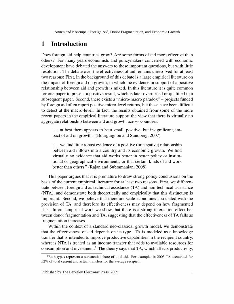
We obtain a similar result when abandoning panel regressions and switching tocross-sectional regressions. In this way we can test for the partial impact of TApc on income growth for the time horizon between 1970 and 2004. However, thedrawback of cross-sectional regressions is that we are no longer able to control forunobserved heterogeneity. In these regressions we include some additional con-trols such as institutional quality (ICRG), ethnic fractionalization, and geographysuch as the percentage of tropical area and an Sub-saharan Africa dummy and anEast Asia dummy. Table 5 shows the cross-sectional results. We present OLS and2SLS results. For the 2SLS result reported in Column (2), we use a similar instru-

19



Table 3: Sensitivity to the Choice of Control Variables

(1) (2) (3) (4)

Initial GDP pc -3.75∗∗∗ -1.78∗∗ -2.84∗∗∗ -3.61∗∗∗(0.97) (0.73) (0.90) (1.26)

Investment/GDP 1.77 3.50∗∗∗ 3.37∗∗∗(1.19) (1.03) (0.79)

Openness 0.028∗ 0.015 0.041∗∗∗(0.016) (0.016) (0.014)

M2/GDP -0.095∗∗∗ -0.098∗∗∗ -0.11∗∗∗(0.016) (0.017) (0.020)

Inflation -0.0011∗∗ -0.0013∗∗ -0.0012∗∗(0.00049) (0.00057) (0.00050)

Budget balance/GDP -0.017 -0.015 -0.012(0.016) (0.018) (0.010)

Revolutions -0.70∗ -1.05∗∗∗ -0.79∗∗(0.38) (0.38) (0.39)

Life expectancy 0.26∗∗∗ 0.19∗∗ 0.29∗∗∗(0.087) (0.088) (0.081)

TA pc 0.060∗∗∗ 0.045∗∗∗ 0.063∗∗∗ 0.050∗∗(0.016) (0.014) (0.016) (0.020)

TA pc × frag. -0.00084∗∗∗ -0.00046∗ -0.00081∗∗∗ -0.00074∗∗(0.00029) (0.00026) (0.00030) (0.00034)


N 621 621 621 621Hansen Over-id test 0.418 0.472 0.363 0.146AB(1) p-value 0 0 0 0AB(2) p-value 0.794 0.804 0.852 0.796Dependent Variable in all equations is average growth rates. Significance levels : ∗ : 10 ∗∗: 5% ∗ ∗ ∗ : 1%. All estimations use the system GMM estimator. Robust standard errors arein parenthesis. Constant term, time-, and country fixed effects are not reported. AB(1) and AB(2)refers to the Arellano-Bond test for first and second order zero autocorrelation respectively.

mentation strategy than the one adopted in Rajan and Subramanian (2008). That iswe use information on the colonial past, common language, and population ratios(as a proxy for donor influence) to predict TA receipts using the dyadic data set ofdonor-recipient pairs.26 The estimation results for the exogenous variation of TA pcby donor across recipients is reported in Table 9 in the Appendix. We then aggregatedonor-recipient aid flows to get one observation of predicted TA pc per recipient.Predicted TA pc is then used as an instrument for actual TA pc. The specification

26The only difference to Rajan and Subramanian (2008) is that we do not use a dummy for coun-tries that are currently in a colonial relationship. Our sample does not include such a country.

20



Table 4: Sensitivity to the Choice of Period Length

(1) (2) (3) (4)

Period Interval 5-years 6-years 8-years 10-years

Initial GDP pc -5.66∗∗∗ -3.49∗∗∗ -2.95∗∗∗ -1.62∗∗(1.47) (1.01) (1.02) (0.81)

Investment/GDP 0.78 1.43 1.45∗ 1.55∗(1.05) (0.97) (0.79) (0.87)

Openness 0.025∗ 0.026∗∗ 0.017 0.019∗(0.013) (0.012) (0.011) (0.011)

M2/GDP -0.042 -0.092∗∗∗ 0.00013 0.011(0.042) (0.020) (0.014) (0.0094)

Inflation -0.00099∗∗∗ -0.0012∗∗ -0.00085∗∗ -0.0012∗∗∗(0.00020) (0.00053) (0.00038) (0.00037)

Budget balance/GDP 0.0036 0.012∗∗∗ 0.050∗∗∗ 0.37(0.011) (0.0042) (0.017) (0.64)

Revolutions -1.21∗∗∗ -0.47 -0.59 -0.15(0.45) (0.41) (0.47) (0.36)

Life expectancy 0.34∗∗∗ 0.22∗∗∗ 0.20∗∗∗ 0.11∗∗(0.086) (0.078) (0.055) (0.054)

TA pc 0.059∗∗∗ 0.049∗∗∗ 0.054∗∗ 0.026(0.019) (0.017) (0.027) (0.020)

TA pc × frag. -0.0011∗∗∗ -0.00081∗∗∗ -0.00095∗∗ -0.00067∗∗(0.00035) (0.00030) (0.00042) (0.00032)

Donor Fragmentation 0.041∗ 0.042∗∗ 0.046 0.016(0.025) (0.021) (0.028) (0.017)

N 498 435 300 289Hansen over-id test 0.300 0.263 0.278 0.479AB(1) p-value 0 0 0.003 0.001AB(2) p-value 0.229 0.046 0.168 0.315Dependent Variable in all equations is average growth rates. Significance levels : ∗ : 10 ∗∗: 5% ∗ ∗ ∗ : 1%. All estimations use the system GMM estimator. Robust standard errors arein parenthesis. Constant term, time-, and country fixed effects are not reported. AB(1) and AB(2)refers to the Arellano-Bond test for first and second order zero autocorrelation respectively.

reported in Column (2) in Table 5 is the one that is closest to the specification re-ported in Rajan and Subramanian (2008). In the specification reported in Column(3) we add the Sub-saharan Africa and the East Asia dummy variables as additionalcontrols as done in Burnside and Dollar (2000). In this latter specification we finda similar result than in the panel estimations. The coefficient for TA pc is positiveand significant and the interaction term is negative and again significant. In Column(4) we add “democracy” from Freedom house as an additional instrument so that

21



−.1

−.0

50

.05

.1

0 20 40 60 80 100Donor Fragmentation

Partial Impact of TA pc from Eq. (4) in Table 5

Figure 3: 95% Confidence Interval of Partial Impact of TA pc

we can run a Hansen over-identification test. We fail to reject the null hypothesisthat our instruments are exogenous, suggesting that our predicted aid variable is avalid instrument.

In order to compare this result with our main result we plot the 95% confidenceinterval in Figure 3. We find a positive and significant positive impact of TA pcon income growth provided that donor fragmentation is low enough – similar thanin Figure 2. In contrast to the panel result plotted in Figure 2, we find that TA pccan actually adversely affect income growth if donor fragmentation is high. Thisevidence suggests that TA pc positively affects economic performance in the short-and long-run provided that donor fragmentation is low enough. In contrast, if donorfragmentation is high, we find no significant impact on income growth in the short-run but a negative impact on income growth in the long-run.

In conclusion, we find evidence that TA pc interacts negatively with donor frag-mentation. The partial impact of TA pc on income growth declines as donor frag-mentation increases. We obtain this result using a range of different estimationprocedures. When we vary the period length, we can learn something about theshort- and long-run impact of TA pc. Here, we find a positive and significant effectof TA pc on income growth provided that donor fragmentation is sufficiently lowin the short- and long-run. This result goes a long with the model’s prediction pre-sented earlier for the case when TA is perceived as being permanent. The reportedevidence, in addition, suggests that TA pc may lower growth rates when donor frag-

22



Table 5: Cross-section 1970-2004

(1) (2) (3) (4)

Estimation method OLS 2SLS 2SLS 2SLS

Initial GDP pc -1.25∗∗∗ -1.25∗∗∗ -1.22∗∗∗ -1.22∗∗∗(0.22) (0.20) (0.18) (0.18)

Investment/GDP 1.05∗∗∗ 1.06∗∗∗ 0.69∗∗ 0.68∗∗(0.31) (0.30) (0.35) (0.34)

Openness (initial) 0.0034∗ 0.0045∗∗∗ 0.0049∗∗∗ 0.0049∗∗∗(0.0019) (0.0016) (0.0014) (0.0014)

M2/GDP (initial) -0.0064∗∗∗ -0.0048∗∗ -0.00097 -0.00094(0.0021) (0.0022) (0.0054) (0.0053)

Inflation (initial) 0.00057 0.00075∗ 0.00064∗ 0.00062(0.00054) (0.00043) (0.00038) (0.00038)

Budget surplus (initial) -0.46∗∗ -0.80∗∗∗ -0.69∗∗∗ -0.65∗∗∗(0.19) (0.25) (0.25) (0.24)

Revolutions 0.18 -0.097 -0.50 -0.49(0.55) (0.56) (0.44) (0.44)

Life expectancy (initial) 0.044 0.023 0.022 0.023(0.028) (0.027) (0.026) (0.025)

Institutional quality (ICRG) 1.69∗∗∗ 1.93∗∗∗ 1.57∗∗∗ 1.54∗∗∗(0.51) (0.59) (0.60) (0.58)

Ethnic fractionalization -1.97∗∗∗ -2.08∗∗∗ -1.63∗ -1.62∗(0.65) (0.72) (0.95) (0.93)

Percentage of tropical area 0.21 0.44 0.18 0.15(0.42) (0.39) (0.41) (0.40)

Sub-Saharan Africa dummy -0.61 -0.63(0.79) (0.76)

East Asia dummy 1.22∗∗ 1.25∗∗∗(0.48) (0.47)

TA pc 0.030∗∗ 0.031 0.033∗∗ 0.035∗∗(0.015) (0.024) (0.016) (0.015)

TA pc × frag. -0.00071∗ -0.0013∗∗∗ -0.0011∗∗∗ -0.0011∗∗∗(0.00037) (0.00044) (0.00034) (0.00033)


N 83 83 83 83R-squared 0.61 0.53 0.61 0.62adj. R-squared 0.53 0.43 0.52 0.53Hansen Over-id test 0.4315Dependent Variable in all equations is average growth rates. Significance levels : ∗ : 10 ∗∗ :5% ∗ ∗ ∗ : 1%. Robust standard errors are in parenthesis. Constant term is not reported.

mentation is high. Particularly in the long run, TA pc seems to affect income growthnegatively for countries with a fragmentation above 53%. In other words, if TA isnot administered efficiently then it may have adverse effects.

23



4.3 Sensitivity to the Normalization of AidThroughout the paper we normalized aid by dividing it by the population of recip-ient countries. To divide aid by GDP, however, is the aid normalization typicallyused in the literature. We prefer to use aid per capita mostly for econometric rea-sons. Dividing aid by GDP introduces an additional potential source for endogene-ity. Table 6 shows the results when using aid divided by GDP instead of aid percapita. TA divided by GDP is positive and significant in all columns, except Col-umn (5). Table 6 is essentially a duplication of Table 3 with the exception that wenow use aid divided by GDP. We can conclude that our main result is robust to theaid normalization used. However, when comparing Table 3 with Table 6 we cansee that in Table 6 the result depends more on the exact specification used. This,however, is expected. Since our aid measure has now being divided by GDP, acountry that performs well will have a low aid divided by GDP value but a highgrowth of income per capita, thereby introducing a downward bias. What Table 6reveals is that if TA/GDP is used then it is particularly important to adequately con-trol for cross country heterogeneity in steady state income levels. The investmentrate, for example, is an important control variable.27 For this reason, our preferredaid normalization is to use aid per capita instead of aid divided by GDP.

5 ConclusionsIn this paper we show, first, that aid effectiveness depends on the type of aid, and,second, that aid effectiveness depends on the fragmentation level of aid. The typeof aid matters because different types of aid enter differently into an economy. Weargued that NTA enters into the economy through the resource constraint. We de-veloped a model that shows that this form of aid may not increase income growth,namely then when perceived as being permanent. TA, however, affects productiv-ity – via human capital production. This type of aid increases income growth bothwhen perceived as being temporary or permanent. In our empirical analysis weshow that NTA does not affect growth rates. In contrast, TA does, provided that its

27Excluding the investment rate lowers the point estimate for TA/GDP, because a positive corre-lation between GDP and income growth and the investment rate respectively means we associatelow aid values with high growth rates or high aid values with low growth rates, thereby introducinga downward bias.

level of fragmentation is sufficiently low. We provide evidence that the effectivenessof TA significantly depends on donor fragmentation. With a low donor fragmenta-tion, the partial impact of TA on income growth is large. For example, increasingTA pc by $10 increases annual growth rates by about 0.6 percentage points if donor

24



Table 6: Sensitivity to the Normalization Choice of Aid

(1) (2) (3) (4) (5)

Initial GDP pc -3.79∗∗∗ -3.52∗∗∗ -0.78 -3.05∗∗∗ -2.68∗∗∗(0.89) (0.91) (0.77) (0.87) (1.02)

Investment/GDP 1.00 1.61 2.93∗∗ 3.26∗∗∗(1.22) (1.29) (1.24) (0.83)

Openness 0.030∗ 0.026 0.019 0.036∗∗∗(0.016) (0.017) (0.018) (0.013)

M2/GDP -0.089∗∗∗ -0.090∗∗∗ -0.094∗∗∗ -0.10∗∗∗(0.017) (0.016) (0.021) (0.017)

Inflation -0.00100∗∗ -0.00087∗∗ -0.0011∗∗ -0.0011∗∗(0.00043) (0.00042) (0.00051) (0.00047)

Budget balance/GDP 0.00048 -0.012 -0.012 -0.0067(0.012) (0.012) (0.016) (0.0074)

Revolutions -0.57 -0.69∗ -1.00∗∗ -0.85∗∗(0.38) (0.40) (0.39) (0.41)

Life expectancy 0.31∗∗∗ 0.29∗∗∗ 0.23∗∗∗ 0.27∗∗∗(0.066) (0.070) (0.072) (0.064)

TA/GDP 234.0∗∗ 253.2∗∗ 278.6∗∗ 281.2∗∗ 184.8(112.8) (121.3) (116.0) (123.7) (118.3)

TA/GDP × frag. -3.41∗∗ -3.72∗∗ -3.74∗∗ -4.03∗∗ -2.70(1.69) (1.73) (1.73) (1.73) (1.67)

NTA/GDP -3.95(15.5)

Donor Fragmentation 0.045 0.042 0.046 0.035 0.034(0.030) (0.033) (0.036) (0.034) (0.033)

N 621 621 621 621 621Hansen over-id test 0.955 0.450 0.310 0.346 0.260AB(1) p-value 0 0 0 0 0AB(2) p-value 0.824 0.778 0.839 0.898 0.812Dependent Variable in all equations is average growth rates. Significance levels : ∗ : 10 ∗∗: 5% ∗ ∗ ∗ : 1%. All estimations use the system GMM estimator. Robust standard errors arein parenthesis. Constant term, time-, and country fixed effects are not reported. AB(1) and AB(2)refers to the Arellano-Bond test for first and second order zero autocorrelation respectively.

fragmentation is zero, whereas this effect drops to 0.15 if donor fragmentation is50%. We find a strong interaction effect between TA and donor fragmentation nomatter the exact specification, time frame, or aid normalization we use.

One of the main conclusions of this paper is that donor fragmentation seems tointroduce inefficiencies thereby significantly reducing the effectiveness of technicalassistance. This paper provides empirical evidence for the view that asks for a bettercoordination among donor countries to improve the effectiveness of foreign aid.

According to growth accounting studies, differences in levels of GDP per per-son between the wealthiest and poorest countries are due primarily to differences inthe production function residual; whereas only a small amount is accounted for by

25



differences in physical capital intensity (see Hall and Jones, 1999). As such, onewould think that the policies that will be most effective in reducing internationalincome disparities will be the ones that help reduce the productivity gap, and bypromoting the accumulation of human capital this is exactly what technical assis-tance is intended to do. This paper demonstrated that when foreign aid takes theform of technical assistance it can be effective at improving economic conditions inpoor countries, at least when it is administered efficiently.

AppendixTable 7: Countries in the Sample

Albania Ghana OmanAlgeria Grenada∗ PakistanArgentina Guatemala Papua New GuineaAzerbaijan Guinea-Bissau ParaguayBahamas, The Haiti PeruBahrain Honduras PhilippinesBangladesh∗∗ India Rwanda∗

Barbados∗ Indonesia Saudi ArabiaBelize∗ Iran, Islamic Rep. SenegalBhutan∗ Jamaica Sierra LeoneBolivia Jordan SingaporeBotswana Kazakhstan SloveniaBrazil Kenya Solomon Islands∗

Burkina Faso Korea, Rep. South AfricaBurundi∗ Kuwait Sri LankaCambodia∗ Kyrgyz Republic∗ St. Kitts and Nevis∗

Cameroon Lebanon St. Lucia∗

Chad∗ Lesotho∗ St. Vincent and the Grenadines∗

Chile Macedonia, FYR∗ SudanChina Madagascar SurinameColombia Malawi Swaziland∗

Congo, Dem. Rep. Malaysia TanzaniaCongo, Rep. Maldives∗ ThailandCosta Rica Mali TogoCote d’Ivoire Malta Tonga∗

Croatia Mauritania∗ Trinidad and TobagoCyprus Mauritius∗ TunisiaDjibouti∗ Mexico TurkeyDominican Republic Moldova UgandaEcuador Mongolia UruguayEgypt, Arab Rep. Morocco Venezuela, RBEthiopia Namibia∗∗ VietnamFiji∗ Nepal∗ Yemen, Rep.Gabon Nicaragua ZambiaGambia, The Niger ZimbabweGeorgia∗ Nigeria∗ and ∗∗ denotes a country when only included in the sample for panel results and cross-sectionresults respectively.

26



Table 8: Data SourceVariable Definition SourceGDP pc GDP per capita PPP adj. Penn World Tables 6.2

in $2000.Investment/GDP Investment share of real Penn World Tables 6.2

GDP in $2000.Openness Exports and Imports divided Penn World Tables 6.2

by real GDP ($2000)M2/GDP M2 dividid by GDP both World Development Indicators

in local current currencyInflation Yearly consumer price World Development Indicators

inflationBudget balance Budget surplus divided by Financial Statistics IMF

GDP both in local currentcurrency or US dollars

Revolutions Number of revolutions Arthur S. Banksper year

Life expectancy Life expectancy at birth World Development Indicatorsin years

TA Technical Cooperation OECD.statPPP in $2000.

NTA See discussion in text OECD.statColony Data on colonial history CEPII Research CenterLanguage Common language CEPII Research CenterPopulation Penn World Tables 6.2Democracy Freedom HouseInstitutional Quality International Country Risk GuideEthnic Fractionalization Philip G. Roeder. 2001.

Ethnolinguistic Fractionalization(ELF) Indices, 1961 and 1985.

Percentage of GEO-data, Gallup, John L.tropical area and Jeffrey D. Sachs (1999)

27



Table 9: Estimation of exogenous variation in TA pc by donors across recipients

Dummy for pairs that ever had a colonial relationship -2.23(2.20)

Dummy for pairs that have common language 2.28∗∗∗(0.57)

Dummy for country that ever had a colonial relationship with U.K. -0.82∗∗∗(0.18)

Dummy for country that ever had a colonial relationship with France -1.05∗∗∗(0.28)

Dummy for country that ever had a colonial relationship with Spain -0.47∗∗∗(0.15)

Dummy for country that ever had a colonial relationship with Portugal 0.38(0.38)

Ratio of logarithm of population of donor relative to recipient 0.56∗∗∗(0.18)

Ratio of logarithm of population × colony dummy 4.69∗∗∗(1.20)

Ratio of logarithm of population × U.K. colony dummy -0.23(0.22)

Ratio of logarithm of population × France colony dummy 0.52(0.36)

Ratio of logarithm of population × Spain colony dummy -0.31(0.30)

Ratio of logarithm of population × Portuguese colony dummy 0.20(0.31)

N 3212R-squared 0.24adj. R-squared 0.23Dependent Variable in all equations is TA pc. Significance levels : ∗ : 10 ∗∗ : 5% ∗ ∗ ∗ :1%. OLS regression. Robust standard errors are in parenthesis. Constant term is not reported.

ReferencesAGENOR, P.-R., N. BAYRAKTAR, AND K. E. AYNAOUI (2008): “Roads out of

Poverty? Assessing the links between Aid, Public Investment, Growth, andPoverty Reduction,” Journal of Development Economics, 86(2), 277–295.

AMEGASHIE, J. A., B. QUATTARA, AND E. STROBL (2007): “Moral Hazardand the Composition of Transfers: Theory with an Application to Foreign Aid,”Working Paper, Department of Economics, University of Guelph.

ARELLANO, M., AND S. BOND (1991): “Some Tests of Specification for PanelData: Monte Carlo Evidence and an Application to Employment Equations,”Review of Economic Studies, 58, 277–297.

BARRO, R. J., AND X. SALA-I MARTIN (2004): Economic Growth. MIT Press,Cambridge, Mass.

28



BLUNDELL, R., AND S. BOND (1998): “Initial Conditions and Moment Restric-tions in Dynamic Panel Data Models,” Journal of Econometrics, 87, 115–143.

BOONE, P. (1996): “Politics and the Effectiveness of Foreign Aid,” European Eco-nomic Review, 40(2), 289–329.

BOURGUIGNON, F., AND M. SUNDBERG (2007): “Aid Effectiveness - Openningthe Black Box,” American Economic Review, 97(2), 316–321.

BRAMBOR, T., W. R. CLARK, AND M. GOLDER (2006): “Understanding Interac-tion Models: Improving Emprical Analyses,” Political Analysis, 14, 63–82.

BURNSIDE, C., AND D. DOLLAR (2000): “Aid, Policies, and Growth,” AmericanEconomic Review, 90(4), 847–868.

CASS, D. (1965): “Optimum Growth in an Aggregate Model of Capital Accumu-lation,” Review of Economic Studies, 32(July), 233–240.

CHATTERJEE, S., S. G., AND S. J. TURNOVSKY (2003): “Unilateral CapitalTransfers, Public Investment and Economic Growth,” European Economic Re-view, 47, 1077–1103.

CHATTERJEE, S., P. GIULIANO, AND K. ILKER (2007): “Where Has All theMoney Gone? Foreign Aid and the Quest for Growth,” IZA-Discussion Paper.

CHATTERJEE, S., AND S. J. TURNOVSKY (2007): “Foreign Aid and EconomicGrowth: The Role of Flexible Labor Supply,” Journal of Development Eco-nomics, 84, 507–533.

CLEMENS, M., S. RADELET, AND R. BHAVNANI (2004): “Counting ChickensWhen They Hatch: The Short Term Effect of Aid on Growth,” Working PaperCenter for Global Development 44.

DALGAARD, C.-J., H. HANSEN, AND F. TARP (2004): “On the Empirics of For-eign Aid and Growth,” Economic Journal, 114, F191–F216.

DEVARAJAN, S., AND V. SWAROOP (1998): “The Implication of Foreign Aid Fun-gibility for Development Assistance,” Policy Research Working Paper Series,World Bank, 2022.

EASTERLY, W. (2003): “Can Foreign Aid Buy Growth?,” Journal of EconomicPerspectives, 17(3), 23–48.

EASTERLY, W., R. LEVINE, AND D. ROODMAN (2004): “Aid, Policies, andGrowth: Comment,” American Economic Review, 94(3), 774–780.

29



GLAESER, E. L., R. LA PORTA, F. LOPEZ-DE SILANES, AND A. SHLEIFER

(2004): “Do Institutions Cause Growth?,” NBER Working Paper, Nr. 10568.

HALL, R. E., AND C. I. JONES (1999): “Why do some Countries Produce so muchmore Output per Worker than others?,” Quarterly Journal of Economics, 114,83–116.

HODLER, R. (2007): “Rent Seeking and Aid Effectiveness,” International Tax andPublic Finance, 14(5), 525–541.

JUDSON, R., AND A. L. OWEN (1996): “Estimating Dynamic Panel Data Mod-els: A Practical Guide for Macroeconomicsts,” Working paper, Federal ReserveBoard of Governors.

KNACK, S., AND A. RAHMAN (2007): “Donor Fragmentation and BureaucraticQuality in Aid Recipients,” Journal of Development Economics, 83(1), 176–197.

KOOPMANS, T. C. (1965): “On the Concept of Optimal Economic Growth,” TheEconometric Approach to Development Planning.

MANKIW, G., D. ROMER, AND D. WEIL (1992): “A Contribution to the Empiricsof Economic Growth,” Quarterly Journal of Economics, 107, 407–37.

MINOIU, C., AND S. G. REDDY (2009): “Development Aid and Economic Growth:A Positive Long-Run Relation,” SSRN eLibrary.

RAJAN, R. G., AND A. SUBRAMANIAN (2008): “Aid and Growth: What does theCross-Country Evidence Really Show?,” The Review of Economics and Statis-tics, 90(4), 643–665.

RAMSEY, F. (1928): “A Mathematical Theory of Savings,” Economic Journal,38(December), 543–559.

RIDDELL, R. (2007): Does Foreign Aid Really Work? Oxford University Press,Oxford.

ROODMAN, D. (2006): “An Index of Donor Performance,” Working Paper Centerfor Global Development, 67.

(2009): “How to do xtabond2: An introduction to difference and systemGMM in Stata,” Stata Journal, 9(1), 86–136.

WOOLBRIDGE, J. (2002): Econometric Analysis of Cross Section and Panel Data.MIT-Press, Boston, Cambridge Mass.

30



Foreign Aid, Donor Fragmentation, and Economic Growth · Volume 9, Issue 1 2009 Article 33 Foreign...

Documents

Transcript of Foreign Aid, Donor Fragmentation, and Economic Growth · Volume 9, Issue 1 2009 Article 33 Foreign...