FORECASTING VALUE-AT-RISK BY USING GARCH MODELS

BY

NASIR ALI KHAN

B.S. (ACTUARIAL SCIENCE & RISK MANAGEMENT)

UNIVERSITY OF KARACHI

February 2007

II

ACKNOWLEDGEMENT Acknowledge is due to Department of Statistics, University of Karachi for support of this

project.

We wish to express our appreciation to Mr. Usaman Shahid who served as advisor, and

has major influence in guiding us in the correct direction of implementing the project.

Specially, I thanks to my taecher Mr. Uzair Mirza for supporting and helping me in

problems I faced during this period.

I would also like to thanks my friends and colleagues who have been of great help by

providing advices to improve our work.

III

ABSTRACT: The variance of a portfolio can be forecasted using a single index model or the covariance matrix of the portfolio. Using univariate and multivariate conditional volatility models, this paper evaluates the performance of the single index and portfolio models in forecasting Value-at-Risk (VaR) of a portfolio by using GARCH-type models, suggests that which model have lesser number of violations, and better explains the realized variation.

IV

TABLE OF CONTENTS 1.0 Introduction ………………………………………………………………1

1.1 Stochastic Process 1.1.1 Stationary time series 1.1.2 Non-stationary time series

1.2 Value-at-Risk 1.3 Conditional volatility model 1.4 Methodology

2.0 Conditional Hetroscedastic Model …………………………………….10

2.1 Introduction 2.2 Assumption for OLS Regression 2.3 Hetroscedasticiy 2.4 Hetroscedastic Model and its specification

2.4.1 ARCH Model 2.4.2 GARCH Model 2.4.3 EGARCH Model 2.4.4 GJR Model

2.5 Parameter Estimation 2.6 Dynamic Conditional Correlations

3.0 Data ………………………………………………………………………20

3.1 Introduction 3.2 KSE-100 Index 3.3 Sample Portfolio

4.0 Pre-Estimation Analysis ………………………………………………...26

4.1 Introduction 4.2 Ljung-Box-Pierce Q-Test 4.3 Engle’ ARCH Test 4.4 Analysis

5.0 Applying Models ………………………………………………………32

5.1 Introduction 5.2 Estimation of Parameter and Conditional Volatility 5.3 Post Estimation Analysis

6.0 Testing of Models ……………………………………………………...40

6.1 Introduction 6.2 Linear Regression Approach 6.3 Back Testing

7.0 Conclusion………………………………………………………………44

V

8.0 Appendices ……………………………………………………………..45 A. Plots B. ACF & PACF Plots of Retorns C. ACF & PACF Plots of Squared Retorns D. ACF & PACF Plots of Absolute Retorns E. Ljung-Box Peirce Q-Test F. Engle’s ARCH Test G. Parameter Estimation H. Linear Regression Approach I. Back Testing J. MATLAB Code

9.0 Biblography …………………………………………………………….79

VI

LIST OF FIGURE 3.1 Daily prices, returns and squared returns of KSE-100 index ….....…………….…..21

3.2 Price trend of six selected stocks .…………………..……………………...………23

3.3 Plot of returns and squared returns of sample portfolio ...……….…………...…….24

4.1 ACF and PACF plot of log returns of KSE-100 index ………….……………...….28

4.2 ACF.and PACF plot of squared returns of KSE-100 index …….……………….....29

4.3 ACF and PACF plot of absolute returns of KSE-100 index …….………………....29

4.4 LBQ-test and ARCH-test of KSE-100 index returns …………….………………...30

4.5 LBQ-test and ARCH-test of KSE-100 index squared returns ………………..…...31

5.1 Estimated coefficient with iterations for GARCH(1,1) specification …...…………34

5.2 Comparison of return, innovations and conditional volatilities ...……………….....36

5.3 Standardized innovations of GARCH(1,1) ………………………………………...37

5.4 ACF plot of squared standardized innovations …………………………………….37

5.5 LBQ-test and ARCH–test for innovations …………………………………………38

6.1 forecasted VaR and violations of upper and lower band………………………...…42

VII

LIST OF TABLES 3.1 portfolio components with their respective sectors, index weights and portfolio weights…22

3.2 Descriptive statistics of index and sample stocks returns …………………………………25

6.1 Number and percentage of violation of VaR bands …...…………………………………..42

1

1.0 INTRODUCTION Conditional variance of the portfolio or stock returns is one of the key ingredients required to calculate the Value-at-Risk (VaR) of a portfolio or any individual stock. Conditional volatility models used to estimate the conditional variance of the portfolio returns either by using a multivariate volatility model to forecast the conditional variance of each asset in the portfolio, as well as the conditional co variances between the assets pair, in order to calculate the forecasted portfolio conditional variance and called the portfolio model; or fitting univaiate volatility model to the portfolio returns, called single index model. Secondly, compare each estimated conditional variance and VaR from different hetroscedastic models and suggests which one model is better explains. In this document, I compare the performance of the KSE-100 index as single index and portfolio, which covers 45% market capitalization of KSE-100 index and contains its six highly traded components, taking as sample. I also compare single index model with same portfolio model. There are different criteria are used to compare the forecasting performance of the various conditional volatility models and methods considered, namely: (1) the linear regression approach of Pagan and Schwert (1990) and (2) backtesting method of Crnkovic and Drachman (1996), applied in J. P. Morgan’s RiskMetrics technical document Engle (2000) proposed a Dynamic Conditional Correlation (DCC) multivariate GARCH model which models the conditional variances and correlations using a single step procedure and which parameterizes the conditional correlations directly in a bivariate GARCH model. In this approach, a univariate GARCH model is fitted to a product of two return series. Parameters or model coefficients of GARCH model can be estimated by log likelihood estimation. The need to model the variance of a financial portfolio accurately has become especially important following the 1995 amendment to the Basel Accord, whereby banks were permitted to use internal models to calculate their Value-at-Risk (VaR) thresholds (see

2

Jorion (2000) for a detailed discussion of VaR). This amendment was in response to widespread criticism that the ‘Standardized’ approach, which banks used to calculate their VaR thresholds, led to excessively conservative forecasts. Excessive conservatism has a negative impact on the profitability of banks as higher capital charges are subsequently required. Although the amendment to the Basel Accord was designed to reward institutions with superior risk management systems, a back testing procedure, whereby the realized returns are compared with the VaR forecasts, was introduced to asses the quality of the internal models. In cases where the internal models lead to a greater number of violations than could reasonably be expected, given the confidence level, the bank is required to hold a higher level of capital. If a bank’s VaR forecasts were violated more than 9 times in any financial year, the bank may be required to adopt the ‘Standardized’ approach. The imposition of such a penalty is severe as it affects the profitability of the bank directly through higher capital charges has a damaging effect on the bank’s reputation, and may lead to the imposition of a more stringent external model to forecast the bank’s VaR.

1.1 STOCHASTIC PROCESS Stochastic or random process is a collection of random variable ordered in time. If we let P denote a random variable, and if it is continuous, we denote as P(t), but if it is discrete, we denoted it as Pt. Economic data and Assets prices, such as daily stock prices, bond prices, foreign exchange rate, GDP, inflation rates etc. are examples of stochastic process and in the discrete form. As we work on equity prices, If Pt denote a stock’s price at time t, where t=1,2,3,….n. stochastic process are two types, stationary and non-stationary stochastic process.

1.1.1 STATIONARY TIME SERIES The foundation of time series is stationary. A time series {rt} is said to be strictly stationary if the joint distribution of (rt1,….,rtk) is identical to that of (rt1+t,….,rtk+t) for all t, where k is arbitrary positive integer and (t1,….tk) is a collection of k positive integers. In other words, a stochastic process is said to be stationary if its mean and variance are constant over time and the value of covariance between the two time periods depends

3

only on the distance or gap or the lag between two time periods and not the actual time at which covariance is computed. A time series {rt} is weakly stationary if both the mean of rt and covariance rt and rt-l, where l is an arbitrary integer. More over rt is weakly stationary if:

( )( ) ( )( ) ( )( )[ ] kkttktt

tt

t

PPEPPCovPEPVar

PE

γμμσμ

μ

=−−==−=

=

++,

2

1.1.2 NON-STATIONARY TIME SERIES

If a time series is not stationary in the sense just defined, it is called non-stationary time

series. In other words, a non-stationary time series will have a time-varying mean or

time-varying variance or both. The classic example of non-stationary time series is

Random Walk Model (RWM). It is often said that asset prices, such as stock prices or

exchange rates, follows a random walk; that is they are non-stationary. There are two

types of random walks:

1. Random walk without drift

2. Random walk with drift

RANDOM WALK WITHOUT DRIFT

Let rt be a white noise with mean 0 and variance σ2. Then the series Pt is said to be

random walk if:

ttt rPP += −1

In random walk model shows that the value of P at time is equal to its value at time t-1

plus a random shock; thus it is an AR(1). Believer in the efficient capital market

hypothesis argue that stock prices are essentially random and no scope for profitable in

the stock markets.

4

In general, if the process started at some time 0 with value of Y0, we have

∑+= tt rPP 0

( ) ( ) 00 PrPEPE tt =+= ∑

( ) 2σtPV t =

RANDOM WALK WITH DRIFT Let

ttt rPP ++= −1μ Where μ is known as drift parameter. We ca also write as

tttt rPP +=− − μ It shows that Pt drift upward or downward, depending on m being positive or negative. It is also an AR(1) model. Where

( ) μtPPE t += 0

( ) 2σtPV t =

RWM with drift the mean as well as the variance increases over time, again violating the conditions of weak stationary. RWM, with or without drift, is a non-stationary stochastic process. 1.2 VALUE-AT-RISK (VaR) When using VaR measure, we are interested in making a statement of the following form. For example:

“We are P% certain that we will not lose more than $V in the next N days.”

5

V is the VaR of the portfolio. It is a function of two parameters: N is the time horizon, and, the confidence level. It is the loss level over N days that the manager is P% certain will not be exceeded. In general, when an N day is the time horizon, and P% is the confidence level, VaR is the loss corresponding to the (100-P)th percentile of the percentile of the distribution of the change in the value of the portfolio over the next N days. VaR is an attractive measure because it is easy to understand. In essence, it asks the simple question “how bad can things get?” All senior mangers want answered this question. A measure that deals with the problem we have just mentioned is conditional VaR (C-VaR). C-VaR “if things do get bad, how much can we expect to lose?” C-VaR is expected loss during an N-days period conditional that we are in the (100-X)% left tail of the distribution. In theory, VaR has two parameters. These are N, the time horizon measured in days, and X, and the confidence interval. In practice, analyst almost invariability set N = 1 in the first instance. The usual assumption is

N-day VaR = 1-day VaR (√N)

This formula is exactly true when the changes in the value of the portfolio on the successive days have independent identical normal distribution with mean zero. In other cases, it is an approximation. There are different methodologies to calculate the VaR, most popular are Historical simulation, Variance – Covariance, Monte Carlo simulation, J. P. Morgan’s RiskMetrics® Methodology etc. Different methodologies have different approaches and different inputs to calculate the VaR of the portfolio, but volatility is the main ingredient to estimate the VaR of an asset. In this technical report, estimate volatility by using RiskMetrics. Actually, this technical report focused on C-VaR or forecasting VaR, so RiskMetrics is specially design for C-VaR. however, volatility is the main ingredient to calculate VaR and conditional VaR depends upon conditional volatility. RiskMetrics uses historical time series analysis to derive estimates of volatilities and correlations on a large set of financial instruments. It assumes that the distribution of past returns can be modeled to provide us with a reasonable forecast of future returns over different horizons. While RiskMetrics assumes conditional normality of returns, we have

6

refined the estimation process to incorporate the fact that most markets show kurtosis and leptokurtosis. We will be publishing factors to adjust for this effect once the RiskMetrics customizable data engine becomes available on the Reuters Web. These volatility and correlation estimates can be used as inputs to:

Analytical VaR models Full valuation models.

Users should be in a position to estimate market risks in portfolios of foreign exchange, fixed income, equity and commodity products.

1.3 CONDITIONAL VOLATILITY MODELS As in technical document, J. P. Morgan’s RiskMetrics (1995) introduced EWMA approach. RiskMetrics uses the exponentially weighted moving average model (EWMA) to forecast variances and covariances (volatilities and correlations) of the multivariate normal distribution. This approach is just as simple, yet an improvement over the traditional volatility forecasting method that relies on moving averages with fixed, equal weights. This latter method is referred to as the simple moving average (SMA) model. To compute exponentially weighted (standard deviation) volatility, formula given as:

∑=

−+ −)−1 =

T

tt

tt rr

1

121 )(( λλσ (1.1)

Consequently, under the EWMA model in Eq. (1.1) the conditional variance or rt is proportional to the time horizon k. The conditional standard deviations of a k-period horizon return k at+1 EWMA is a special form of heteroscedastic model IGARCH(1,1) with intercept equal to zero, today’s GARCH-type models have gained the most attention, because that time series realization of returns often show time-dependent volatility. This idea was first give in Engle’s (1982) ARCH (Auto Regressive Conditional Heteroscedasticity) model, which is base on the specification of conditional densities at consecutive periods with a time

7

dependent volatility process. Volatility compute by these models is easy; it is two-step regression model on assets returns. Then we will also work on GARCH models, which are advance shape of ARCH model, which firstly introduced by Bolerslev, T. in his journal of Econometrics, “Generalized Auto Regressive Conditional Hetroscedasticity” in 1986, other are GJR, EGARCH, IGARCH, and etc. the detail discussions about each model will be in next chapter. EWMA is special form of IGARCH(1,1) without drift or with intercept 0.

1.4 METHODOLOGY

Risk is often measured in terms of price changes. These changes can take a variety of forms such as absolute price change, relative price change, and log price change. When a price change is defined relative to some initial price, it is known as a return. RiskMetrics measures change in value of a portfolio (often referred to as the adverse price move) in terms of log price changes also known as continuously compounded returns. For any asset, we know the price, for example at time t is Pt of an asset, and its current price is Pt+1, so the absolute return, Ra, for an asset at time t from t+1 is given as:

tta PPR −= + 1 (1.2)

Where a in the subscript of R is referring to absolute, relative price change or return, Rr, relative to price Pt:

t

ttr P

PPR −= + 1

(1.3)

Then the log price change or continuously compounded return, rt+1, of a security is defined to be the natural logarithm of its gross return.

8

⎟⎟⎠

⎞⎜⎜⎝

⎛=

+=

+

t

t

r

PPr

Rr

1ln

)1ln(

( ) ( )ttt PPr lnln 11 −= ++ (1.4)

We firstly compose the portfolio, give weights each with respect its market capitalization

and KSE-100 index acts as single or index, which discuss in detail in chapter 3. In

chapter 4, now we check each time series of stocks return that model which we have

discussed in chapter 2 are applicable or not. For this, we use three methods, ACF and

PACF, Ljung-Box-Perice Q-Test and Engle’s ARCH Test; apply on returns and squared

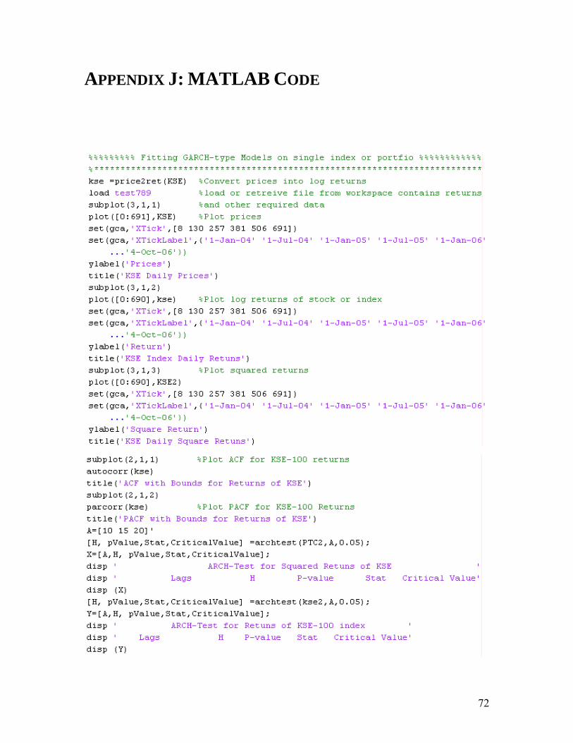
returns and absolute. In chapter 5, by using MATLAB 7.0 commands, estimate the

parameter or coefficients of each of the given models, MATLAB commands and code are

given in the appendix J that used for this paper and then test the outputs. In the next

chapter, assessing the each model by to approaches, linear regression approach and back

testing. In regression approach, apply simple linear regression on each model variance by

taking independent variable, squared returns as dependent, check coefficients, and

coefficient of determination under the assumptions of OLS model. On the other hand,

back testing on each model and confirm the number of VaR violations. Suppose that the

financial position is a long position so that loss occurs when there is a big price drop. If

the probability is set to 5%, then RiskMeterics uses 1.65σt+1 to measure the risk of the

portfolio-that is, it uses the one sided 5% quantile of a normal distribution with mean and

variance 0 and σt+1. The actual 5% quantile is -1.65σt+1, but the negative sign is ignored

with the understanding that it signifies a loss. Consequently, if the standard deviation is

measured in percentage, the daily VaR of the portfolio under RiskMeterics is:

VaR = (Amount of Position) (1.65σt+1)

In addition, that of a k-day horizon is

VaR = (Amount of Position) (1.65σt+1)

9

Where the argument (k) of VaR is used to denote the time horizon. We have

VaR =√ k x VaR

This is referred to as the square root of time rule in VaR calculation under RiskMetreics.

10

2.0 CONDITIONAL HETEROSCEDASTIC

MODELS 2.1 INTRODUCTION Econometricians are typically to determine how much one variable will change in response to a change in some other variable. Increasingly however, econometricians are being asked to forecast and analyze the size of the errors of the model. In this case, the questions are about volatility, and the standard tools have become the ARCH/GARCH models.

2.2 ASSUMPTIONS FOR OLS REGRESSION OLS (ordinary least square) regression analysis is the great workhorse of economists and statisticians and forms a central tool in financial modeling. The well-proved technique relies on a set of four basic underlying assumptions to produce linear models that are the Best Unbiased Linear Estimate (BLUE). Furthermore, it is necessary to add a fifth assumption of homoscedasticity to obtain results that are also statistically consistent. It is assume that there are linear parameters, meaning that there is a linear relationship between the dependent and the explanatory variables. Mathematically this relationship is expresses as a function of the form:

uXY ++= 10 ββ (2.1)

Where β0 is the intercept, β1 the slope of the function and where u represents an error term containing all the factors affecting Y other than the specified independent variable. Second, it is intuitively a necessity that the sample to be analyzed must consist of a random sample of the relevant population to yield an unbiased result. Mathematically (xi,

11

yi): i = 1, 2...n. Third, a zero conditional mean is assumed. This means that the linear model will be the single line that minimizes the value of the sum of all error terms forming an average of the positive and negative errors. In other words, this means that the average error term of the function should always be zero as the negative and positive errors cancel each other out. This can be refined into the assumption that the average value of u does not depend on the value of X as for any value of X the average value of u will be equal to the average value of u in the entire population, which is zero. Mathematically it can Econometricians are typically to determine how much one variable will change in response to a change in some other variable. Increasingly however, econometricians are being asked to forecast and analyze the size of the errors of the model. In this case, the questions are about volatility, and the standard tools have become the ARCH/GARCH models be expressed as:

( ) ( ) 0| == uExuE

Fourth, it is assumed a sample variation in the independent variables X. This means that two independent variables cannot be equal to the same constant. This is however not an assumption that is likely to fail in an interesting statistical analysis as a completely homogenous population is not the typical target for statistical analysis. The assumption is defined as xi, i = 1, 2...n. These assumptions assure an unbiased result where the sample βn is equal to the population βn. Finally, we assume homoscedasticity to obtain a consistent result. This assumption states that the value of the variance of error term u conditional on the explanatory variable X is constant. In other words, the pattern of distribution of error terms at any given value of X will show the same distribution with a mean around the sample βnX. This is expressed as:

2)|( σ=xuVar

2.3 HETROSCEDASTICITY The effect of a violation of this assumption is that we still have a BLUE model, however it is no longer consistent and, as a result the regression output in terms of test statistics can no longer be reliable. This is because the variance that is in the heart of these statistics is no longer constant and will hence be false.

12

In cross sectional data the distribution of the error term u should constant distribution in

relation to the function uXY ++= 10 ββ . Heteroscedasticity in time series will take a

graphically different appearance is that the variance, or the volatility, will vary according to time. Engle (1982) and others with him have looked at the properties of the volatility of financial markets and there is wide recognition of the presence of heteroscedasticity in the distribution of returns. Mandelbrot (2002) describes this phenomenon as a clustering of volatility where a period of high volatility is likely to be followed by another period of high volatility and opposite. The sometimes calm and sometimes turbulent volatilities observed in financial markets. Research has found out that a relationship between volatility from one period to the next one exists. The presence of this heteroscedastic relationship may be used when modeling and forecasting future volatility of financial markets. The range and complexity of methods applied to this problem is vast.

2.4 HETERSCEDASTIC MODELS AND ITS SPECIFICATION Simply using all past information on past price movements does in fact utilize the heteroscedastic properties of financial markets to some extent. By using the formula

( )∑=

−−

=N

tt rr

N 1

2

11σ (2.2)

The assumption that all past prices have an equal relevance in the shaping of the Volatility of the future is applied. Intuitively this assumption is too crude as more recent volatility is likely to have more relevance than that of several years ago and should hence be given a relatively higher weight in the calculation. A simple way to counter this problem is done by only using the last 30 days to calculate the historical volatility and this model is actually widely used by actors in the financial markets. The model weighs volatility older than 30 days as zero and puts equal weight on the volatility of the last 30 days. This model is however still crude and more sophisticated models are frequently used moving into the area covered by models such as the Exponential Weighted Volatility models (EWMA) as shown in Eq (1.1).

13

Models that can be used to estimate the conditional variance of a portfolio directly by modeling the historical stock or portfolio returns or indirectly by modeling the conditional variance of each asset and the conditional correlation of each pair of assets (namely, the portfolio model) are shown in this section. Financial returns are typically modeled as a stationary AR(1) process.

2.4.1 ARCH MODEL Prior to the ARCH model introduced by Engle (1982), the most common way to forecast volatility was to determine the standard deviation using a fixed number of the most recent observations. As we know that the variance is not constant, i.e. homoscedastic, but rather a heterocedastic process, it is unattractive to apply equal weights considering we know recent events are more relevant. Moreover, it is not beneficial to assume zero weights for observations prior to the fixed timeframe. The ARCH model overcomes these assumptions by letting the weights be parameters to be estimated thereby determining the most appropriate weights to forecast the variance. An ARCH(1) model, where the conditional variance depends only on one lagged square error, is given by

2

1102

−+= tt δαασ (2.3)

We can capture more of the dependence in the conditional variance by increasing the number of lags, p , giving us an ARCH( p ) model

22

222

1102

ptpttt −−− ++++= δαδαδαασ L (2.4) 2.4.2 GARCH MODEL Bollerslev in 1986 proposed a useful extension known as the Generalized Autoregressive Conditional Heteroscedasticity (GARCH) model. For a log return rt. Let at be the mean corrected log return. If δt follows a GARCH(u, v) model is:

14

ttt εσδ = ∑ ∑= =

−− ++=u

i

v

jjtjitit

1 1

220

2 σβδαασ (2.5)

Since, we know that r t is log return of daily stock prices with mean, μ=0 and we also know that δt is mean corrected return and can be written as:

μδ −= tt r

Where δt is a random variable with mean 0 and variance 1, and assumed to be standard normal or standardized student-t distribution. If v=0, then equation (2.5) reduces to ARCH(u). Simplest form of GARCH model is GARCH(1,1), and written as

2

12

102

−− ++= ttt βσαδασ (2.6)

Where, ( ) 1,1,0 <+≤≤ βαβα

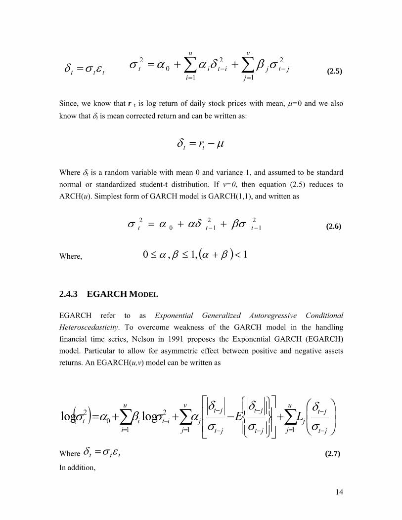
2.4.3 EGARCH MODEL EGARCH refer to as Exponential Generalized Autoregressive Conditional Heteroscedasticity. To overcome weakness of the GARCH model in the handling financial time series, Nelson in 1991 proposes the Exponential GARCH (EGARCH) model. Particular to allow for asymmetric effect between positive and negative assets returns. An EGARCH(u,v) model can be written as

( ) ∑∑ ∑= −

−

= = −

−

−

−− ⎟

⎟⎠

⎞⎜⎜⎝

⎛+

⎥⎥⎦

⎤

⎢⎢⎣

⎡

⎪⎭

⎪⎬⎫

⎪⎩

⎪⎨⎧

−++=u

j jt

jtj

u

i

v

j jt

jt

jt

jtjitit LE

11 1

20

2 loglogσδ

σ

δ

σ

δασβασ

Where ttt εσδ = (2.7)

In addition,

15

( ) {tsStudent

GaussianEE

jt

jtjt '

/2

2

21

2

π

υ

υ

πυσ

δε

⎟⎠⎞

⎜⎝⎛Γ

⎟⎠⎞

⎜⎝⎛ −

Γ−−

−− =

⎟⎟⎠

⎞⎜⎜⎝

⎛=

As the range of log (σt) is the real number line, the EGARCH model does not require any parametric restrictions to ensure that the conditional variances are positive. Furthermore, the EGARCH specification is able to capture several stylized facts, such as small positive shocks having a greater impact on conditional volatility than small negative shocks, and large negative shocks having a greater impact on conditional volatility than large positive shocks. Such features in financial returns and risk are often cited in the literature to support the use of EGARCH to model the conditional variances.

2.4.4 GJR MODEL Glosten, Jagannathan and Runkle (1992) extended the GARCH model to capture possible asymmetries between the effects of positive and negative shocks of the same magnitude on the conditional variance through changes in the debt-equity ratio. The GJR(u,v) model is given by:

( ) ∑∑

=−

=−−− +++=

v

iiti

u

jttjtjt D

11

211

20 σβδψγδαασ

(2.8)

Where ttt εσδ = and indicator or dummy variable, D (ψτ−1), is defined as

( ) 01

00{ ≤>= tif

iftD δδψ

For the case u = 1, a0>0, α1>0, α1+γ1 >0, β1 ≥0 are sufficient conditions to ensure a strictly positive conditional variance, σt>0. The indicator variable distinguishes between positive and negative shocks, where the asymmetric effect ( γ1 > 0 ) measures the contribution of shocks to both short run persistence (α1 +γ1 / 2 ) and long run persistence (α1 +β1 +γ1 / 2). Several important theoretical results are relevant for the GARCH model.

16

Ling and McAleer (2002) established the necessary and sufficient conditions for strict stationarity and ergodicity, as well as for the existence of all moments, for the univariate GARCH( u,v ) model, and Ling and McAleer (2003) demonstrated that the QMLE for GARCH( u, v ) is consistent if the second moment is finite, E(δ2)<∞, and asymptotically normal if the fourth moment is finite, E(δ4)<∞. The necessary and sufficient condition for the existence of the second moment of δt for the GARCH(1,1) model is α1 +β1 <1. Another important result is that the log-moment condition for the QMLE of GARCH(1,1), which is a weak sufficient condition for the QMLE to be consistent and asymptotically normal, is given by E(log(αtψt

2+β1)). The log-moment condition was derived in Elie and Jeantheau (1995) and Jeantheau (1998) for consistency and in Boussama (2000) for asymptotic normality. In practice, it is more straightforward to verify the second moment condition than the weaker log-moment condition, as the latter is a function of unknown parameters and the mean of the logarithmic transformation of a random variable. The GJR model has also had some important theoretical developments. In the case of symmetry of ψt, the regularity condition for the existence of the second moment of GJR(1,1) is α1+β1+γ1/2<1 (see Ling and McAleer (2002)). Moreover, the weak log moment condition for GJR(1,1), E(log[(α1+γ1D(ψt))ψt

2+β1 ])< 0, is sufficient for the consistency and asymptotic normality of the QMLE (see McAleer, Chan and Marinova (2002)). 2.5 PARAMETERS ESTIMATION Historical observations will be used to estimate the parameters in these models. The approach used to estimate the parameters is the maximum likelihood method. It involves choosing values for the parameters that maximize the chance (or likelihood) of the data occurring. The first assumption made, is that the probability distribution of εi conditional on the variance is normal. In Hull (2003) the best parameters can be found by maximizing

17

⎟⎟⎠

⎞⎜⎜⎝

⎛ −

=∏

2

2

2

122

1 i

i

em

i t

σδ

πσ (2.9)

Where m is the number of observations. Maximizing an expression is equivalent to maximizing the logarithm of the expression. Taking the logarithm of the expression in equation (2.7) and ignoring constant multiplicative factors, it can be seen that we wish to maximize.

∑

=⎟⎟⎠

⎞⎜⎜⎝

⎛−−

m

i t

it

12

22ln

σδσ

An iterative search is used to find the parameters in the model that maximize the expression in equation (2.9).

2.6 DYNAMIC CONDITIONAL CORRELATION A new class of multivariate GARCH estimators which can best be viewed as a generalization of Bollerslev(1990)’s constant conditional correlation estimator. In

ttt RDDH =

Where { }tit hdiagD ,=

Where Ht is conditional covariance matrix and R is a correlation matrix containing the conditional correlations as can directly be seen from rewriting this equation as:

[ ] RDHDE tttttt == −−−

111 'εε

Since ttt D δε 1−=

18

The expressions for h are typically thought of as univariate GARCH models; however, these models could certainly include functions of the other variables in the system as predetermined variables or exogenous variables. A simple estimate of R is the unconditional correlation matrix of the standardized residuals. Engle’s (2000) proposes an estimator called Dynamic Conditional Correlation or DCC. The dynamic correlation model differs only in allowing R to be time varying:

tttt DRDH = Parameterizations of R have the same requirements that H did except that the conditional variances must be unity. The matrix Rt remains the correlation matrix. Probably the simplest specification for the correlation matrix is the exponential smoother, which can be expressed as:

∑∑

∑−

=−

−

=−

−

= −=1

1,

1

1,

,1

1 ,, t

titj

t

titi

ijt

t ititij

ελε

ελερ

A geometrically weighted average of standardized residuals. Clearly, these equations will produce a correlation matrix at each point in time. A simple way to construct this correlation is through exponential smoothing. In this case the process followed by the

( )( ) ( )1,1,1,, 1 −−− +−= tijtjtitij qq λεελ

tjjtii

tijtij qq

q

,,

,, =ρ

19

A natural alternative is suggested by the GARCH(u, v) model.

∑ ∑= =

−−− ++=u

m

v

nntnmtmtmtij qq

1 10, βεεαα

Matrix versions of these estimators can be written as:

( )( ) 111 '1 −−− +−= tttt QQ λεελ

and 111 )'()1( −−− ++−−= tttt QSQ βεεαβα

where S is the unconditional correlation matrix and Qt is covariance matrix. So, GARCH models can also be used for updating covariance estimates and forecasting the future level of covariance. For example, the GARCH(1,1) model for updating a covariance and simply write as is

Cov t = α0 +α1 ri,t-1 r j,t-1 +βCov t-1

In addition, the long-term average covariance is α0 / (1−α1+β1).

20

3.0 DATA

3.1 INTRODUCTION For this study, I select KSE-100 Index stocks of Karachi Stock Exchange. My main objective is not only to forecast conditional volatilities or to suggest which model better explains the given data, but I also want to study the behavior of our local markets. We can also implement on the other financial and economic time series data, such are foreign exchange rate, bonds or fixed income securities, etc. but for ARCH/GARCH model require large sample size data and it cannot easily available. 3.2 KSE-100 INDEX Karachi Stock Exchange is the biggest and liquid exchange and has been declared as the “Best Performing Stock Market of the World for the year 2002”. As on June 30, 2006, 658 companies were listed with the market capitalization of Rs. 2,801.182 billion (US $ 46.69) having listed capital of Rs. 495.968 billion (US $ 8.27 billion). KSE began with a 50 shares index. On November 1, 1991 the KSE-100 was introduced and remains to this date the most generally accepted measure of the Exchange. The KSE-100 is a capital-weighted index and consists of 100 companies representing about 90 percent of market capitalization of the Exchange. KSE-100 index is weighted average of 100 stock prices on Karachi Stock Exchange and is therefore good benchmark for KSE. The KSE-100 Index closed at 9989.41 on June 30, 2006. Karachi Stock Exchange recently introduced KSE-30 index, last year. As we see in figure 3.1, KSE-100 index have increasing trend from Jan 2004 to Oct 2006. There some fluctuation in KSE-100 between Jan and Jul in both year 2004 and 2005, KSE-100 rapidly increases and drop, known as March Crisis. KSE-100 index average returns are zero throughout the graph; there are huge fluctuations and deviations between

21

Jan and Jul in 2004 and 2005. The main purpose of square returns plot to analyze the variation in the returns of index.

Figure 3.1: Daily prices, returns and squared returns of KSE-100 index.

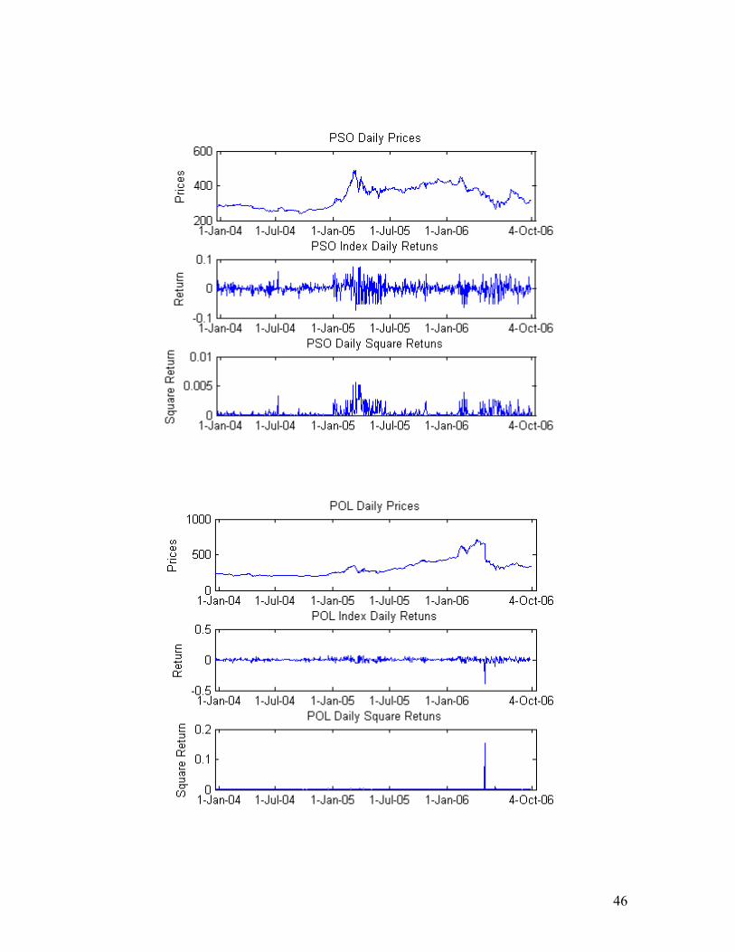
The data used for this study consists of stock prices from six different companies and the price of the index itself, selection based on market capitalization. The prices are corrected for stock splits and dividend. The daily closing prices were retrieved dated from 22 Dec 2003 to Oct 2006. This means that the dataset consists of 692 observations for each company and the index itself. The mixture of six different stocks called Portfolio.

3.3 SAMPLE PORTFOLIO OGDC is on number one of the list of KSE-100 index, because of its huge market capitalization, its weight is 20%, KSE-100 compose on the basis of Market capitalization and its market capitalization is about Rs. 50, 707, 946, 000. On the second number, Pakistan Telecommunication, the biggest telephone service provider, only fixed landline telephone service provider in the country and have large customers. Their subsidiaries are

22

Ufone (Cell phone service Provider), Paknet (Internet service provider) and V-PTCL (based on WLL technology). National Bank is the biggest bank in Pakistan, which management is completely own by the public sector. The MCB Bank Limited is one of the largest banks in Pakistan. MCB, advised by Merrill Lynch, became the fourth Pakistani company (the other three being Hubco, PTCL and Chakwal Cement - they all have been de listed) to list on the London Stock Exchange when it raised $150 million floating global depositary receipts. MCB Bank Ltd. ranks amongst the Leaders in the commercial banking industry. MCB has been one of the most profitable banks of 2005, registering an increase of over 250% in net profits. POL is a petroleum exploration and production company. The company also own and operates a network of pipelines for transportation of crude oil to Attock Refinery Limited in Rawalpindi. POL has two subsidiaries. One subsidiary CAPGAS markets LPG and another subsidiary Attock Chemical produces sulphuric acid. Pakistan State Oil (PSO) is the oil market leader in Pakistan. The well-established infrastructure, built at par with international standards, representing 82% of country’s storage, provides PSO an edge over its competitors. PSO is currently enjoying over 73% share of Black Oil market and 59% share of White Oil market. It is engaged in import, storage, distribution and marketing of various petroleum products including mogas, high speed diesel (HSD), fuel oil, jet fuel, kerosene, liquefied petroleum gas (LPG), compressed natural gas (CNG) and petrochemicals. PSO also enjoys around 35% market participation in lubricants.

Table 3.1: Sample portfolio components with their respective sectors, index weights and portfolio weights.

23

Figure 3.2: price trend of six selected stocks.

As we see in figure 3.2, stocks price prices moves in horizontal direction form jan 2004 to Jan 2005 as well as KSE-100 also move in the same in the same direction. Nevertheless, after Jan 2004 all stock prices rapidly increased, PTC and MCB have very small effect of it. Stocks that have Massive change in prices all are from oil and gas sector, except NBP. Therefore, this gain in prices is not due to demand and supply or change in prices of petroleum product in domestic and international market, this is rumor which made by some big market player. If compare both figures 3.1 and 3.3, portfolio’s squared returns are greater as compare to square return of KSE-100 index. Therefore, portfolio, which composed, is more volatile than KSE-100 index, because KSE-100 is hundred shares portfolio, more diversified and of course, it has less return. However, trend in both are identical, sample portfolio contain contains those stocks which are actively trade in a market and these stocks have huge average daily trading volume.

24

Figure 3.3: Plot of returns and squared returns of sample portfolio.

We assume log returns are random variable or white noise, which are normally distributed with mean 0 and variance, say σ2. As we see in table 3.2 that all mean of log returns are significantly close to zero and some exactly equal to zero, like PTC and PSO. Variances of stock’s log returns are approximately same, .001. We know that kurtosis of normal distribution is 3. POL log returns are not normally distributed, because its kurtosis is much greater than normal kurtosis and other kurtosis are significantly close to 3. All medians are close to its corresponding means. All returns are negatively skewed, but close to symmetric except POL is more negatively skewed, Skewness is -4.42. Finally, I suggest that all log returns are normally distributed with mean and median close to zero, all variances are similar and symmetric except POL returns. All of six stocks are good correlated to KSE-100 index. As KSE-100 20% depends on OGDC and its correlation is close to zero, 0.877. In addition, correlations among stocks are normally between 0.5 and 0.7. as we compare figure 3.1 and 3.3, price trend of KSE-100 and portfolio are same and same movement of returns and squared returns. So we say that portfolio follow the same trend and behavior as KSE-100 and portfolio is true sample of KSE-100 index.

25

Table 3.2: Descriptive statistics of index and sample stocks returns.

Table 3.3: Correlations among stocks and index.

26

4.0 PRE-ESTIMATION ANALYSIS

4.1 INTRODUCTION

To justify modeling the returns by a GARCH model, the presence needs to be detected first. To detect the presence of a GARCH process, some qualitative and quantitative checks can be performed on the dataset. To check it qualitatively, plots will be made of the sample autocorrelation function (ACF) and the partial-autocorrelation function (PACF) on the returns, looking for signs of correlation. For quantitative checks, two tests will be employed, Ljung-Box-Pierce Q-Test and Engle's ARCH Test.

4.2 LJUNG-BOX-PIERCE Q-TEST The Ljung-Box Pierce Q-Test (LBQ Test) can verify, at least approximately, if a significant correlation is present or not. It performs a lack-of-fit hypothesis test for model misspecification, which is based on the Q-statistic.

( )∑

= −+=

L

k

k

kNr

NNQ1

2

)(2

(4.1)

Where N = sample size, L = number of autocorrelation lags included in the statistic, and r2

k is the squared sample autocorrelation at lag k. Once you fit a univariate model to an observed time series, you can use the Q-statistic as a lack-of-fit test for a departure from randomness. The Q-test is most often used as a post estimation lack-of-fit test applied to the fitted innovations (i.e., residuals). In this case, however, you can also use it as part of the prefit analysis because the default model assumes that returns are just a simple

27

constant plus a pure innovations process. Under the null hypothesis of no serial correlation, the Q-test statistic is asymptotically Chi-Square distributed.

4.3 ENGLE'S ARCH TEST As for Engle's ARCH Test, the ARCH test also tests the presence of significant evidence in support of GARCH effects (i.e. heteroskedasticity). It tests the null hypothesis that a time series of sample residuals consists of independent identically distributed (i.i.d.) Gaussian disturbances, i.e., that no ARCH effects exist. Given sample residuals obtained from a curve fit (e.g., a regression model), this test tests for the presence of uth order ARCH effects by regressing the squared residuals on a constant and the lagged values of the previous M. squared residuals. Under the null hypothesis, the asymptotic test statistic, T(R2) , where T is the number of squared residuals included in the regression and R2 is the sample multiple correlation coefficients, is asymptotically chi square distributed with M degrees of freedom. When testing for ARCH effects, a GARCH(u,v) process is locally equivalent to an ARCH(u+v) process. All the analysis about pre estimation analysis were did in MATLAB 7.0, Q-statistics or Engle’s ARCH-statistics, p-value and critical values at 95% confidence level for 10, 15 and 20 lags are generated in MATLAB. Both functions return identical outputs. The first output, H, is a Boolean decision flag. H = 0 implies that no significant correlation exists (i.e., do not reject the null hypothesis). H = 1 means that significant correlation exists (i.e., reject the null hypothesis). The remaining outputs are the P-value (p-Value), the test statistic (Stat), and the critical value of the Chi-Square distribution (Critical Value).

4.4 ANALYSIS As we can see ACF and PACF plots of KSE-100 index in figure 4.1, 4.2 and 4.3, which shows that there are no autocorrelation or no significant serial correlation and independent. PACF of log returns are give different result, at lag 1 returns are good correlated and till lag 4 PACF shows significant positive serial correlation. Both these plots are useful preliminary identification tools as they provide some indication of the broad correlation characteristics of the returns. Form ACF of log returns, we suggest that no auto correlation is present in returns data. ACF of squared returns are shows that there

28

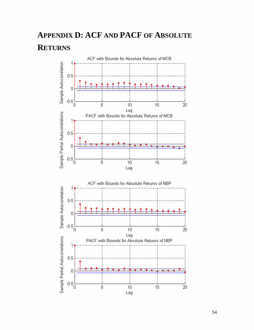
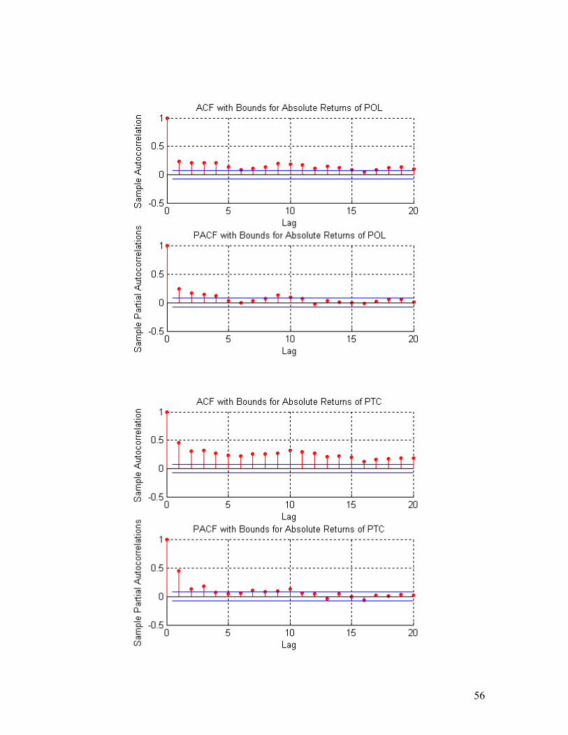
are serial correlation and dependent. We deduce that squared returns are variance process of the returns and PACF of squared returns give the same result. ACF of absolute returns also shows in the figure 4.3 that is significantly serially correlated and dependent. ACF and PACF of returns, squared an absolute returns of each of the six stocks are give in the appendix. ACF’s of each of the stock shows the similar phenomena as KSE-100. ACF of each of the stock shows that returns are not correlated and independent. While ACF’s of stock returns are correlated except POL and NBP. However, ACF of absolute return of all six stocks shows that there is serial correlation and dependent. Lastly, I suggest that all are serially dependent and volatility models, i.e. ARCH and GARCH model are applicable and attempt to capture such dependence in the return series.

Figure 4.1: ACF and PACF plot of log returns of KSE-100 index.

29

Figure 4.2: ACF and PACF plot of squared returns of KSE-100 index.

Figure 4.3: ACF and PACF plot of absolute returns of KSE-100 index.

30

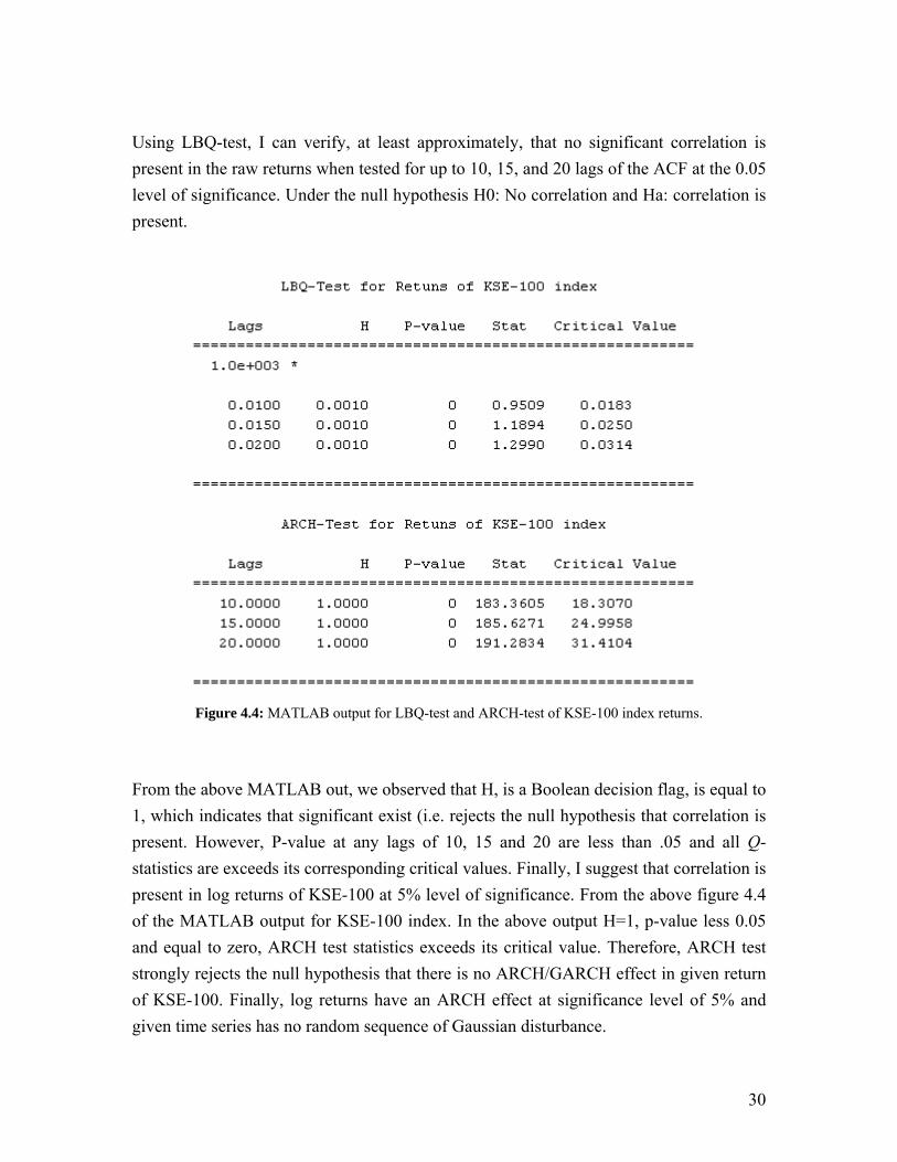
Using LBQ-test, I can verify, at least approximately, that no significant correlation is present in the raw returns when tested for up to 10, 15, and 20 lags of the ACF at the 0.05 level of significance. Under the null hypothesis H0: No correlation and Ha: correlation is present.

Figure 4.4: MATLAB output for LBQ-test and ARCH-test of KSE-100 index returns.

From the above MATLAB out, we observed that H, is a Boolean decision flag, is equal to 1, which indicates that significant exist (i.e. rejects the null hypothesis that correlation is present. However, P-value at any lags of 10, 15 and 20 are less than .05 and all Q-statistics are exceeds its corresponding critical values. Finally, I suggest that correlation is present in log returns of KSE-100 at 5% level of significance. From the above figure 4.4 of the MATLAB output for KSE-100 index. In the above output H=1, p-value less 0.05 and equal to zero, ARCH test statistics exceeds its critical value. Therefore, ARCH test strongly rejects the null hypothesis that there is no ARCH/GARCH effect in given return of KSE-100. Finally, log returns have an ARCH effect at significance level of 5% and given time series has no random sequence of Gaussian disturbance.

31

Figure 4.4: MATLAB output for LBQ-test and ARCH-test of KSE-100 index squared returns.

Same analysis for the squared returns of KSE-100. All H is equal to 1, simply we can serial correlation is present in the squared returns. We further analyzed that P-value for any lag are zero, null hypothesis (H0) cannot be accept at any significance level. Q-statistics at lags 10, 15 and 20 exceeds its corresponding critical values. Therefore, serial correlation is present in the squared returns of KSE-100.

32

5.0 APPLYING MODELS

5.1 INTRODUCTION In the previous chapter, we analyzed the nature of time series. First, we do qualitative test by plotting ACF and PACF of each return or squared return series and check the quality of time series, that they are serially correlated or independent. For further analysis, we quantify the preceding qualitative checks for correlation (ACF and PACF) using formal hypothesis tests, such as the Ljung-Box-Pierce Q-test and Engle's ARCH test. Ljung-Box-Pierce Q-test implemented to check the randomness of the time series data and suggested that correlation is significant or not. In Engle's ARCH test, check the presence of ARCH effects. In this chapter, we will estimate the parameters of the ARCH/GARCH models, which discussed in the second chapter. The parameters of GARCH models can be estimated by maximum likelihood estimation technique (MLE), which is discussed in the as chapter 2. Practically, I use packages, like MATLAB 7.0 and Eveiws for parameter estimation and its analysis. The presence of heteroscedasticity, shown in the previous chapter, indicates that GARCH modeling is appropriate. Use the estimation MATLAB function to estimate the model parameters. I cannot discuss every model for each of the time series. For illustration, I talk about KSE-100 index return series.

5.2 ESTIMATION OF PARAMETER AND CONDITIONAL VOLATILITY

By using MATLAB commands and enter the return series as input and estimates the parameters of a conditional variance specification of GARCH, EGARCH, or GJR form. The estimation process infers the innovations (i.e., residuals) from the return series, and fits the model specification to the return series by maximum likelihood. MATLAB commands related to GARCH are give in Appendix J. Estimated coefficients and

33

MATLAB output for GARCH(1,1) specification with iteration are given in the below figure:

34

Figure 5.1: MATLAB output shows estimated coefficient with iterations for GARCH(1,1) specification.

Generalized form of GARCH(u,v) can be write as:

211

2110

2−− ++= ttt σβδαασ

Where LVγα =0

35

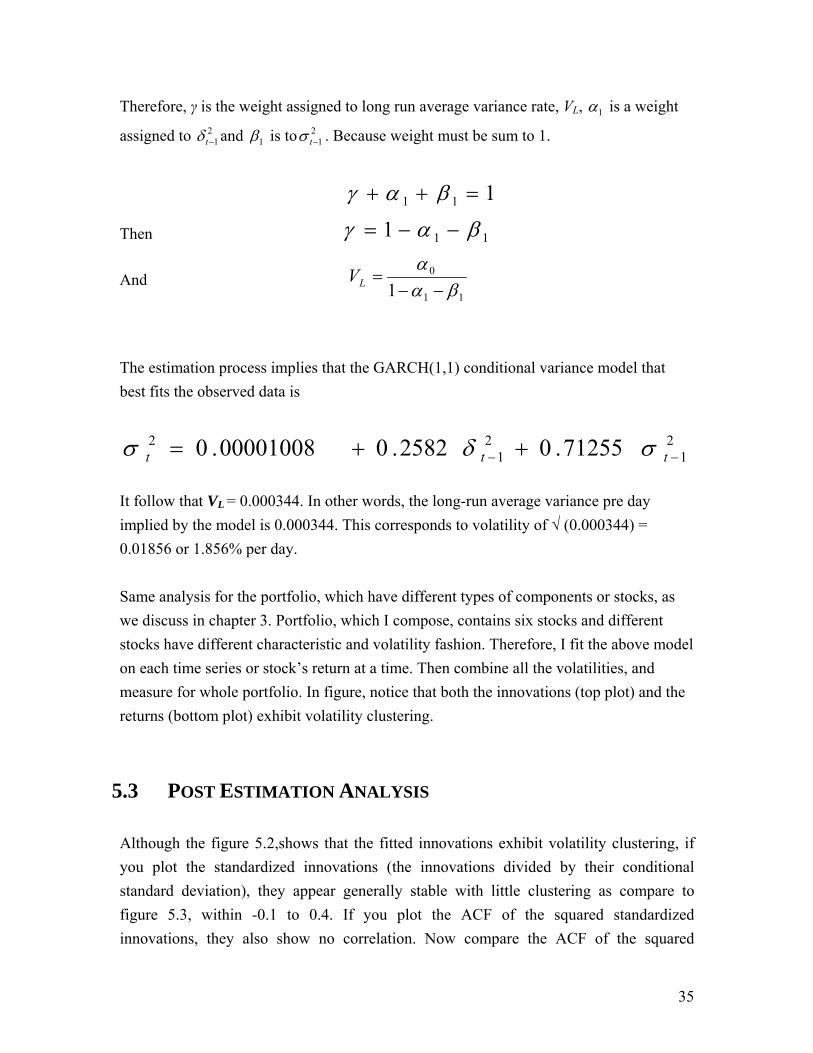
Therefore, γ is the weight assigned to long run average variance rate, VL, 1α is a weight

assigned to 21−tδ and 1β is to 2

1−tσ . Because weight must be sum to 1.

111 =++ βαγ

Then 111 βαγ −−=

And 11

0

1 βαα

−−=LV

The estimation process implies that the GARCH(1,1) conditional variance model that best fits the observed data is

21

21

2 71255.02582.000001008.0 −− ++= ttt σδσ It follow that VL = 0.000344. In other words, the long-run average variance pre day implied by the model is 0.000344. This corresponds to volatility of √ (0.000344) = 0.01856 or 1.856% per day. Same analysis for the portfolio, which have different types of components or stocks, as we discuss in chapter 3. Portfolio, which I compose, contains six stocks and different stocks have different characteristic and volatility fashion. Therefore, I fit the above model on each time series or stock’s return at a time. Then combine all the volatilities, and measure for whole portfolio. In figure, notice that both the innovations (top plot) and the returns (bottom plot) exhibit volatility clustering.

5.3 POST ESTIMATION ANALYSIS Although the figure 5.2,shows that the fitted innovations exhibit volatility clustering, if you plot the standardized innovations (the innovations divided by their conditional standard deviation), they appear generally stable with little clustering as compare to figure 5.3, within -0.1 to 0.4. If you plot the ACF of the squared standardized innovations, they also show no correlation. Now compare the ACF of the squared

36

standardized innovations in figure 5.4 to the ACF of the squared returns prior to fitting the GARCH(1,1) figure 4.2 (chapter 4). The comparison shows that the model sufficiently explains the heteroscedasticity in the raw returns. Compare the results below of the Q-test and the ARCH test with the results of these same tests in the pre estimation analysis (chapter 4). In the pre estimation analysis, both the Q-test and the ARCH test indicate rejection (H = 1 with P-value = 0) of their respective null hypotheses, showing significant evidence in support of GARCH effects. In the post estimation analysis, using standardized innovations based on the estimated model, these same tests indicate acceptance (H = 0 with highly significant P-values) of their respective null hypotheses as shown in figure 5.4 and 5.5 and confirm the explanatory power of the GARCH(1,1) model.

Figure 5.2: comparison of return, innovations and conditional volatilities from GARCH(1,1) model.

37

Figure 5.3: standardized innovations of GARCH(1,1).

Figure 5.4: ACF plot of squared standardized innovations.

38

Figure 5.5: LBQ-test and ARCH–test for innovations.

39

6.0 Testing of Models

6.1 INTRODUCTION After applying different models, next step is to check which is appropriate. In last chapter, we show step of estimation of the model and show only GARCH(1,1) for the purpose of illustration. There are different ARCH/GARCH-type model can be applied on the data which are discussed in the chapter 2, i.e. ARCH, GARCH, EGARCH, GJR models, some of them shown in the appendix with their estimated coefficients. There are different approaches to check which model better explains our stock exchange data. Each model can be applied with different parameters, i.e. u and v, but in limited way, each parameter cannot be greater than three for ARCH and simple GARCH models and two for EGARCH and GJR models. However, I apply different models with different combinations of parameters; they have different characteristics and volatility forecasts, analyze them and identify the causes of difference in them. Two different criteria are used to compare the forecasting performance of the various conditional volatility models and methods considered, namely: (1) the linear regression approach of Pagan and Schwert (1990); (2) RiskMetrics approach of Crnkovic and Drachman (1996).

6.2 LINEAR REGRESSION APPROACH Pagan and Schwert (1990) proposed a procedure whereby the volatility forecasts are regressed on the realized volatility. In this paper, the squared portfolio returns are used as a proxy for the realized volatility. The auxiliary regression equation is given by:

ttt eFVRV ++= βα

40

Where RVt is the realized volatility and FVt is the forecasted volatility. In this auxiliary equation, the intercept, α, should be equal to zero and the slope, β, should be equal to 1. The coefficient of determination, R2, is a measure of forecasting performance, and the t-ratio of the coefficients is a measure of the bias. Tables H-1 and H-2 in appendix give the estimates and test statistics for the single index and portfolio models. Based on the R2 criterion, the portfolio EGARCH(2,1) model performs the best, with R2 = 0.29079 and single index EGARCH(1,2), which R2 = 0.34885 with little difference. The worst performing models are the KSE-100 (single) index ARCH(1) and portfolio EGARCH(2,2) models, which have R2 = 0.02845 and 0.18765 respectively. On the basis of coefficients, intercept terms of all models are same to each other or close to zero. However, on th basis of slope, KSE-100’s EGARCH(2,1) and portfolio’s EGARCH(2,2) with slopes 0.92954 and 1.69581 respectively. In all cases, the single index models outperform the portfolio models based on R2 , which suggests that the index model approach leads to superior forecasts of the conditional variance of the single index compared with their portfolio counterparts.

6.3 BACK TESTING The purpose of this section is not to offer a review of the quantitative measures for VaR model comparison. There is a growing literature on such measures and we refer the reader to Crnkovic and Drachman (1996) for the latest developments in that area. Instead, we present simple calculations that may prove useful for determining the appropriateness of the models.

6.3.1 PORTFOLIO For back testing, I use same index (KSE-100) and portfolio, which contains six stocks with different weights. Using daily prices for the period December 22, 2003 through October 4, 2006 (a total of 962 observations), we construct 1-day VaR forecasts over the most recent 962 days of the sample period. We then compare these forecasts to their respective realized profit/loss (P/L) which are represented by 1-day returns.

41

∑=

=6

1,,

itiitp rwr

Where r i,t represents the log return of the ith stock. The Value-at-Risk bands are based on the portfolio’s standard deviation. The formula for the portfolio’s variance at t is:

Where is the σ2

i,t variance of the ith return series made for time t and γij,t is the correlation between the ith and jth returns for time t and wi is the weight for the ith stock.

6.3.2 ASSESSING THE MODELS The first measure of model performance is a simple count the number of times that the VaR estimates “under predict” future losses (gains). Each day it is assumed that there is a 5% chance that the observed loss exceeds the VaR forecast. For the sake of generality, let’s define a random variable X(t) on any day t such that X(t) = 1 if a particular day’s observed loss is greater than its corresponding VaR forecast and X(t) = 0 otherwise. We can write the distribution of X(t) as follows

( ) { 1,0)()05.01(05.00

)(1)(

05.0|)( =− −

= tXtXtX

tXf e.w

Now, suppose we observe X(t) for a total of T days, t = 1,2,..., T , and we assume that the X(t)’s are independent over time. In other words, whether a VaR forecast is violated on a particular day is independent of what happened on other days. The random variable X(t) is said to follow a Bernoulli distribution whose expected value is 0.05.The total number of VaR violations over the time period T is given by

∑ ∑∑= = >

+=6

1

6

1,

2,

22, 2

i i ijtijjitiitp www γσσ

42

∑=

=T

tT tXX

1)(

The expected value of, i.e., the expected number of VaR violations over T days, is T times 0.05. For example, if we observe T = 961 days of VaR forecasts, then the expected number of VaR violations is (961) (0.05) = 48; hence one would expect to observe one VaR violation every 961 days. What is convenient about modeling VaR violations according to Eq. 6.1 is that the probability of observing a VaR violation over T days is same as the probability of observing a VaR violation at any point in time, t . Therefore, we are able to use VaR forecasts constructed over time to assess the appropriateness of the models for this portfolio of 6 stocks. For example, if we forecast VaR for KSE-100 by the GARCH(1,1) conditional variance model . If true probability of violation is 5%, then realized VaR violations are:

-0.08

-0.06

-0.04

-0.02

0

0.02

0.04

0.06

0.08

KSE

SD-1.65

SD+1.65

Figure 6.1: forecast VaR for KSE-100 by the GARCH(1,1) and violations of upper and lower band.

Table 6.1: No. and percentage of violations of upper and lower band.

43

At confidence level of 95%, we expect that there is 5% chances that VaR band of each side and the expected number of violation is 48 days out of 961 days, violation of lower band closer to expected, of upper band lesser than expected. VaR violation for other models is given in Appendix I.

44

7.0 CONCLUSION The Endeavour to examine if GARCH-type models were the better model in describing return series for VaR was done statistically and empirically. The dataset was first tested by various statistical testing methods to see if GARCH modelling was suitable. Only for NBP and POL, the tests showed showed that there is no significant correlation. The other companies including the KSE-100 index contained correlation in its returns or squared returns, which meant that a GARCH process was found and modeling with GARCH was appropriate. After testing the dataset, the models were set up and run; the parameters were estimated for each of the model with their conditional volatility. As the conditional volatility is the main ingredient for forecasting VaR and its depends on Conditional variance. Then we check the quality of our estimated parameter and volatility. First test the innovations of each, that there are any kind of correlation is present or not. I found that there is no significant correlation and ARCH effect is not present. In the next step, check the conditional volatility by applying linear regression approach that each model can explains market variation. Therefore, models for single-index that are good fitted and better explain the market variation as compare to portfolio, its coefficients of determination are high, beta coefficient close to 1 and a smaller amount of standard errors. In back testing, test the number of violations of VaR band for each model at 95% confidence level. I observed that there is huge number of violations of portfolio VaR and the number of violation of KSE index of its VaR band, close and within its expected violation. In whole document, we assume that KSE-100 index as single index. However, I also compose six and twenty components of single index as well as portfolio of twenty stocks and applying univariate and multivariate model on single index and portfolio respectively. It is observed that single index of six and twenty stocks has less number of violation and close to its expected violations as compare to its portfolios. In addition, it is also observed that the number of stocks increases in the portfolio, so the number of violation also increases as we can see in appendix figure

45

APPENDIX A:

46

47

48

APPENDIX B: ACF AND PACF OF RETURNS

49

50

51

APPENDIX C: ACF AND PACF OF SQUARED

RETURNS

52

53

54

APPENDIX D: ACF AND PACF OF ABSOLUTE

RETURNS

55

56

57

APPENDIX E: LJUNG-BOX-PIERCE Q-TEST OF

RETURNS AND SQUARED RETURNS

58

59

60

APPENDIX F: ENGLE’S ARCH TEST

61

62

63

APPENDIX G: PARAMETER ESTIMATION

(1)

(2)

(3)

64

(4)

(5)

(6)

65

(7)

(8)

(9)

66

APPENDIX H: LINEAR REGRESSION APPROACH

Table H-1: linear regression approach for single index model (KSE-100)

67

Table H-2: linear regression approach for portfolio by using multivariate model

68

APPENDIX I: BACK TESTING

Table I-1: No. and percentage of violations of upper and lower VaR band of single index model(KSE-100)

-0.1000000

-0.0800000

-0.0600000

-0.0400000

-0.0200000

0.0000000

0.0200000

0.0400000

0.0600000

0.0800000

0.1000000

KSE

SD-1.65SD+1.65

Figure I-1: violations of upper and lower VaR band of single index model (KSE-100)

69

Table I-2: No. and percentage of violations of upper and lower VaR band of Portfolio

-0.10000

-0.08000

-0.06000

-0.04000

-0.02000

0.00000

0.02000

0.04000

0.06000

0.08000

port_retSD-1.65SD+1.65

Figure I-2: violations of upper and lower VaR band of Portfolio

70

-0.1

-0.08

-0.06

-0.04

-0.02

0

0.02

0.04

0.06

0.08

SD-1.65SD+1.65Portfolio (20)

Figure I-3: violations of upper and lower VaR band of Portfolio of 20 components by using multivariate

model (example)

Table I-2: No. and percentage of violations of upper and lower VaR band of Portfolio of 20 components by

using multivariate model (example)

-0.10000

-0.08000

-0.06000

-0.04000

-0.02000

0.00000

0.02000

0.04000

0.06000

0.08000

0.10000

PORTFOLIO (6)

SD-1.65

SD+1.65

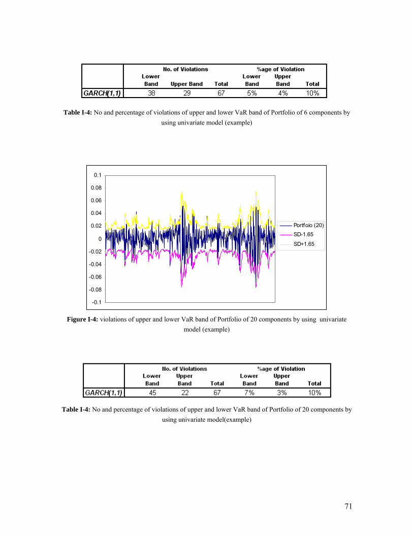
Figure I-4: violations of upper and lower VaR band of Portfolio of 6 components by using univariate

model (example)

71

Table I-4: No and percentage of violations of upper and lower VaR band of Portfolio of 6 components by

using univariate model (example)

-0.1

-0.08

-0.06

-0.04

-0.02

0

0.02

0.04

0.06

0.08

0.1

Portfoio (20)SD-1.65

SD+1.65

Figure I-4: violations of upper and lower VaR band of Portfolio of 20 components by using univariate

model (example)

Table I-4: No and percentage of violations of upper and lower VaR band of Portfolio of 20 components by

using univariate model(example)

72

APPENDIX J: MATLAB CODE

73

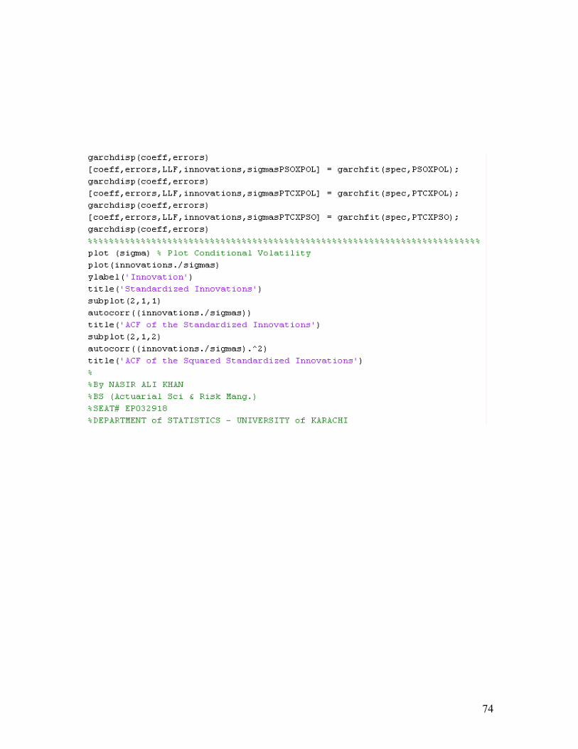
74

75

8.0 BIBLIOGRAPHY Tsay, Ruey S. Analysis of Financial Time Series, First Edition. John Wiley & Sons, INC (2002) Gujrati, Demodar N. Basic Econometrics, Fourth Edition. McGraw Hill International (2003) Longerstaey, Jacques, and Peter Zangari. RiskMetrics™—Technical Document. 4th Edition. (New York: Morgan Guaranty Trust Co., 1996) Engle, Robert. Journal of Economic Perspectives—Volume 15, Number 4—Fall 2001—Pages 157–168 Veiga, Bernardo da & McAleer, Michael Single Index and Portfolio Models for Forecasting Value-at-Risk Thresholds. School of Economics and Commerce, University of Western Australia (January 2005) Hull, John.C. Options, Futures, and Other Derivatives, fifth edition, Prentice Hall International. (2003).