
FORECASTING TOURIST DEMAND TO SINGAPORE: A …vuir.vu.edu.au/15622/1/Kon_2002compressed.pdf ·...
196
FORECASTING TOURIST DEMAND TO SINGAPORE: A MODERN TIME-SERIES APPROACH Sen Choeng Ken A dissertation submitted in partial fulfillment of the requirements for the degree of Doctor of Business Administration School of Applied Economics Faculty of Business and Law Victoria University October 2002
Transcript of FORECASTING TOURIST DEMAND TO SINGAPORE: A …vuir.vu.edu.au/15622/1/Kon_2002compressed.pdf ·...
FORECASTING TOURIST DEMAND TO SINGAPORE:
A MODERN TIME-SERIES APPROACH
Sen Choeng Ken
A dissertation submitted in partial fulfillment
of the requirements for the degree of
Doctor of Business Administration
School of Applied Economics
Faculty of Business and Law
Victoria University
October 2002

WJH^THESIS 338.47915957 KON 30001008249320 Kon, Sen Choeng Forecasting tourist demand to Singapore : a modern time-series approach

ABSTRACT
This dissertation exammes the application of modem time series
forecasting methods in the forecasting of inbound tourists from the six
major tourist generating markets to Singapore, namely the USA,
Ausfralia, Japan, UK, India and China. The purpose of the study is to
assess the capacity of modem time-series models with regard to their
relative forecasting accuracy.
The modem time-series forecasting models applied are Neural
Networks and the Basic Stmctural Model. The time period for the
analysis is from 1985 Quarter 1 to 2001 Quarter 4. The time series are
disaggregated into Holiday, Business, and Total tourist arrivals into
Singapore. Multi-step, one one-step and 4-step ahead forecasts are
made. The forecasting performance comparison between the modem
time-series models are compared using the mean absolute percentage
error (MAPE), against the Winters model and the naive process.
The empirical results show that Neural Networks outperform the BSM
and Winters for the Holiday, Business and Total flows with the Direct
multistep forecast. The BSM outperforms the Neural Network model
and Winters model for one-step-ahead and four-step-ahead forecasts.
The findings indicate that the Neural Network model is an excellent
and practical time-series model for forecasting disaggregated tourist
flows.
Overall, the study vigorously tested the Neural Networks and BSM
modem time series models, and demonstrates their superiority for
tourism demand forecasting over simpler time-series methods, and
highlights to the business practitioner the importance of these models
for short-term tourism demand forecasting.

TABLE OF CONTENTS
CHAPTER 1 INTRODUCTION 1
Introduction 1
1.1 OBJECTIVE OF THE RESEARCH 3
1.2 OUTLINE OF THE THESIS 5
1.3 TOURISM OVERVIEW 7
1.3.1 The Tourism Product 7
1.3.2 The Tourism Industry 8
1.3.3 Tourism Models 9
1.3.4 Tourism Marketing 10
1.3.5 Tourism Demand 13
1.4 ECONOMIC IMPACTS OF TOURISM 15
1.4.1 Tourism Planning and Development 17
1.5 TOURISM IN SINGAPORE 20
1.5.1 Singapore History and Economic Development 20
1.5.2 Economic Importance of Tourism in Singapore 23
1.5.3 Tourism Grov rth 23
1.5.4 Inbound Tourism Market Characteristics 27
1.5.5 Tourism Development 31
CHAPTER 2 LITERATURE REVIEW 38
Introduction 38
2.1 QUALITATIVE FORECASTING METHODS N 40
2.1.1 Jury of Executive Opinion 40
2.1.2 Delphi Method ' 41
2.1.3 Surveys 42
2.2 QUANTITATIVE FORECASTING METHODS 44
2.2.1 Causal Methods 44
2.2.1.1 Regression analysis 44
2.2.1.2 Error Correction Models 55

Ill
2.2.1.3 Multivariate Structural Model 57
2.2.2 Time Series Forecasting Methods 59
2.2.2.1 Naive Forecasting Method 60
2.2.2.2 Simple Moving Average Method 60
2.2.2.3 Decomposition Model 61
2.2.2.4 Exponential Smoothing Methods 62
2.2.2.5 Box-Jenkins Method 66
2.2.2.6 Basic Structural Time Series Models 76
2.2.2.7 Neural Netv*/orks 80
CHAPTERS FORECASTING PROCESS 91
Introduction 91
3.1 THE FORECASTING PROCESS 91
3.1.1 Design 91
3.1.2 Specification 96
3.1.3 Implementation 97
3.1.4 Evaluation 97
CHAPTER 4 EMPIRICAL RESULTS 99
Introduction 99
4.1 FORECASTING PERFORMANCE EVALUATION 99
4.1.1 Forecasting Accuracy Measures 100
4.2 FORECASTING IMPLEMENTATION AND EVALUATION 102
4.2.1 Naive Model 103
4.2.2 Winters Forecasting 105
4.2.3 BSM Forecasting 110
4.2.4 Neural Network Forecasting 115
4.3 FORECASTING ACCURACY COMPARISON 125
CHAPTERS CONCLUSIONS, IMPLICATIONS AND FUTURE RESEARCH 142
5.1 CONCLUSIONS 142
5.2 PRACTICAL CONTRIBUTIONS 144

IV
5.3 RECOMMENDATIONS FOR FUTURE RESEARCH 145
REFERENCE
APPENDICES
147
Appendix A:
Appendix B:
Tourist Flows Data Series Time plots for Australia, China, India, Japan, UK and USA
RMSE values of MLP and RBF Neural Network models
for Australia, China, India, Japan, UK and USA
seasonal data series
Appendix C: RMSE values of MLP and RBF Neural Network models
for Australia, China, India, Japan, UK and USA
deseasonalised data series

LIST OF TABLES
Table 1.1 International Tourist arrivals by Region (mil)
Table 1.2 Variables influencing tourism demand
1
14
Table 1.3 Singapore Tourism Receipts (1990 to 2000)
Table 1.4 Visitor Arrivals to Singapore (1978 to 2000)
23
24
Table 1.5 Percentage Distribution of Regions by Visitor
Arrivals by Residence (1990 to 2000)
Table 1.6 Percentage Distribution of USA, Japan, China,
India, UK and Australia By Visitor Arrivals
by Residence (1990 to 2000)
Forecast Arrivals of USA, Japan, China, India, UK
and Australia from (2002 to 2004)
Percentage Distribution of Visitor Arrivals by
Purpose of Visit
Strategic Plan for Grov rth (1993 to 1995)
ARMA models decision matrix
Forecasting Error Measures
Forecasting Framework
Forecasting implementation of the naive mode!
Summary of Naive Forecast MAPEs
Forecasting implementation of the Winters model.
Winters exponential smoothing forecasting model
example: UK Holiday tourism to Singapore
27
Table 1.7
Table 1.8
Table 1.9
Table 2.1
Table 4.1
Table 4.2
Table 4.3
Table 4.4
Table 4.5
Table 4.6
27
29
29
33
71
100
102
103
104
105
106
Table 4.7 Summary of Winter's Forecast MAPEs 109
VI
Table 4.8 Forecasting implementation of the BSM model 110
Table 4.9 BSM forecasting model example:
Australia Business Travel to Singapore 111
Table 4.10 Summary of Basic Structural Model Forecasts
MAPEs 114
Table 4.11 MLP and RBF Neural Network model parameters 116
Table 4.12 Overall Best Performing Neural network models
- Seasonal Data 120
Table 4.13 Overall Best Performing Neural network models
- Deseasonalised Data 121
Table 4.14 Forecasting implementation of the Neural Network
models 122
Table 4.15 Summary of Neural Networks Forecast MAPEs
- Deseasonalised Data 123
Table 4.16 Summary of Neural Networks Forecast MAPEs
- Seasonal Data 124
Table 4.17 Forecasting Accuracy Comparison of Naive, Winters,
BSM and Neural Networks Models using MAPE 125
Table 4.18 Summary of Holiday Flow MAPEs 131
Table 4.19 Summary of Business Flow MAPEs 132
Table 4.20 Summary of Total Flow MAPEs 133
Table 4.21 Overall average MAPEs for Holiday, Business and Total Flows 137
Table 4.22 Summary of overall average MAPEs for Neural Network models with
seasonal and deseasonalised data 139

Vll
LIST OF FIGURES
Figure 1.1 Seasonality of Arrivals into Singapore for 1999 and 2000 30
Figure 2.1 Types of forecasting methods 39
Figure 3.1 Ex ante/ex post forecasts 97

VIU
DECLARATION
This thesis contains no material which has been accepted for the award of any other
degree or diploma in any university or other institution, and to the best of my
knowledge, contains no material previously published or written by another person,
except where due reference is made in the text of this thesis.
Signed:

IX
ACKNOWLEDGEMENTS
I would like to express my utmost gratitude to my principal supervisor, Professor
Lindsay Turner, who has guided, assisted and encouraged me throughout each stage
of my research. His critical and insightfijl comments have provided thoughtfiil ideas
that have greatly improved the quality of the thesis.
I would also like to thank all the staff in the Faculty of Business, School of Applied
Economics of Victoria University for their helpfiil assistance and care given to me
during my stay in Melbourne, Australia.
Last but not least, I would like to thank my parents, my sisters and my wdfe for their
support and encouragement during this period of research.
CHAPTER 1 INTRODUCTION
Introduction
The rapid growth of international tourism arrivals worldwide has been impressive
since the end of the Second World War. According to the World Tourism
Organisation (WTO), international tourist arrivals grew by 7.4% in 2000, and world
inbound tourism receipts for 2000 totalled US$455.4 billion. Factors that contributed
to worldwide tourism growth are: (a) on the supply side - lower fransportation costs,
government reforms, deregulation and opening of tourist and related sectors; (b) on
the demand side - changing demography with ageing and retirement, global business
fravel, rising affluence, new forms of tourism such as eco-tourism, arts tourism,
religious and adventure tourism.
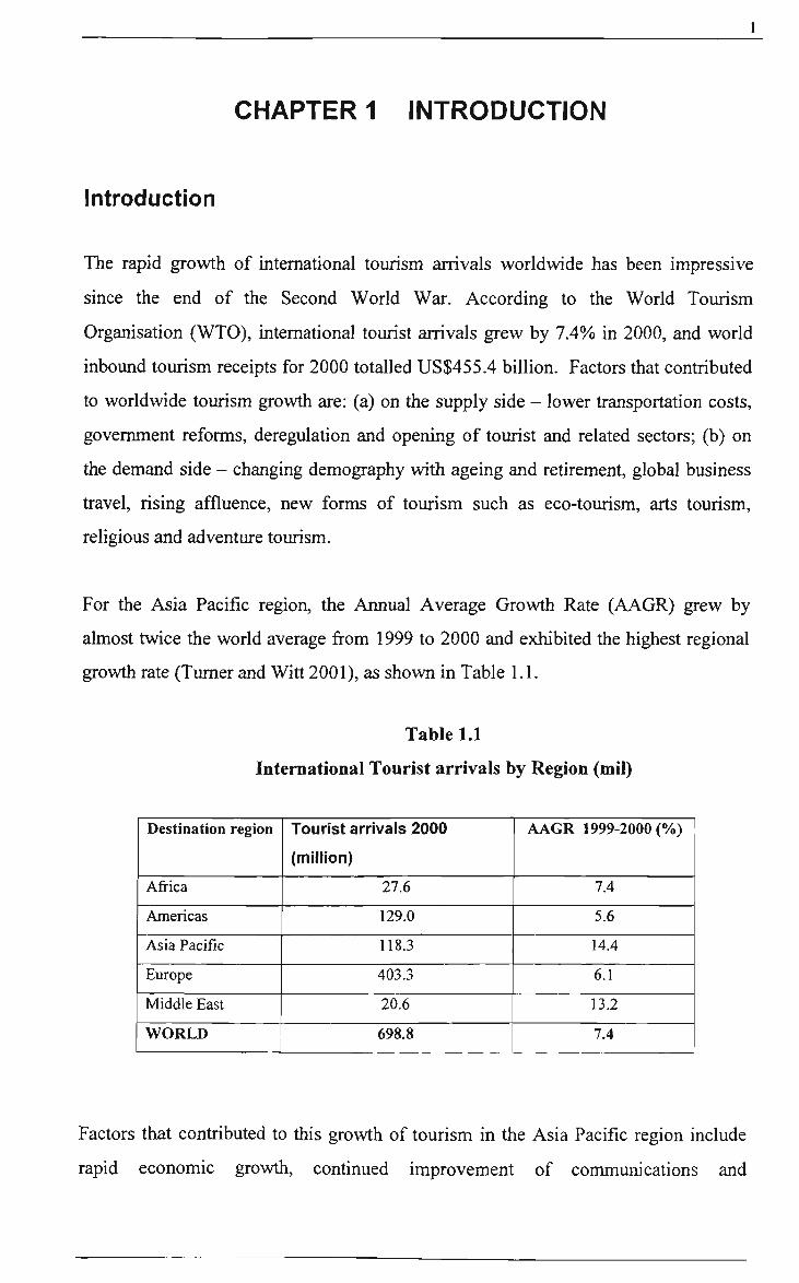
For the Asia Pacific region, the Aimual Average Growth Rate (AAGR) grew by
almost twice the world average from 1999 to 2000 and exhibited the highest regional
growth rate (Turner and Witt 2001), as shown in Table 1.1.
Table 1.1
International Tourist arrivals by Region (mil)
Destination region
Africa
Americas
Asia Pacific
Europe
Middle East
WORLD
Tourist arrivals 2000
(million)
27.6
129.0
118.3
403.3
20.6
698.8
AAGR 1999-2000 (%)
7.4
5.6
14.4
6.1
13.2
7.4
Factors that contributed to this growth of tourism in the Asia Pacific region include
rapid economic growth, continued improvement of communications and

transportation modes, higher per capita personal disposable incomes and more short-
haul intra-regional travel. These factors have resulted in tourism becoming a major
component of economic development and an important source of foreign exchange for
many of the countries in the region. This has raised the intensity of competition in the
tourism industry in the Asia Pacific region as coimtries become more aggressive in
their tourism marketing and promotion campaigns. At the same time, visitors will be
looking for new, exciting and different holiday experiences while choosing from a
wider selection of tourist destinations. This increased growth and competition for
international tourism (Wahab and Cooper 2001) in the Asia Pacific region, and the
importance and contribution of tourism to Singapore's economic performance that is
discussed later highlight the need for accurate tourism demand forecasts for
Singapore.
The importance of tourism demand forecasting is emphasised by Frechtling (1996)
with the following reasons: (a) The perishable nature of the tourism 'product' (Archer
1987), (b) People are inseparable fi-om the production-consumption process, (c)
Customer satisfaction depends on complementary services, (d) Leisure tourism
demand is extremely sensitive to natural and manmade disasters, and (e) Tourism
supply requires large, long lead-time investments in plant, equipment and
infrastmcture. At present, the residual effects of terrorism fears, conflicts and
economic uncertainty in the US, Europe and Middle East is seen to have an affect on
the tourism industry in 2002.
Witt et al. (1991) states: 'Reliable forecasts of tourism demand are essential for
efficient planning by airlines, shipping companies, railways, coach operators,
hoteliers, tour operators, food and catering establishments, providers of entertainment
facilities, manufacturers producing goods primarily for sale to tourists, and other
industries connected with the tourism market.' Tourism demand forecasting models
have been reviewed by Crouch (1994) who found that nearly two-thirds of them
define demand in terms of arrivals or departures; and about one-half of them measured
demand in terms of tourism expenditures and receipts. Frechtling (1996) states that
visitor arrivals in a country or local area constitute tourism demand since visitors avail
themselves of the services of a destination in arriving there. In essence, the availability
of accurate tourist arrivals forecasts can assist governments in tourism planning and
development for the tourism industry.
This study is a significant contribution to the current literature by examining and
testing modem time-series forecasting models for generating accurate disaggregated
tourist arrival forecasts, in the short-term.
1.1 Objective of the Research
Questions relating to the best methodology to use in forecasting tourism arrivals have
been discussed extensively in the literature (Martin and Witt 1989; Crouch and Shaw
1990; Witt and Witt, 1992; Witt et al. 1994). There are basically two kinds of
methods: time-series and causal methods. Each method has different strengths and
weaknesses. The causal models require the need to identify and forecast independent
variables in the defined model in order to use the model. This represents a significant
challenge as the incorrect prediction of these independent variables will result in an
incorrect forecast from the causal model. Moreover, the causal based methodologies
have become very complex in recent years with the use of cointegration modelling and
hence very expensive for use by business. Time-series methods do not have the above
causal requirements and can be more practical for business use, primarily because they
cost less to execute within a business workplace. Furthermore, purely from the point
of view of accuracy, time-series models can be at least as accurate as causal models in
the short term. So in cases where practical forecasting of arrivals numbers is the
primary aim (as opposed to determining cause) time-series models are very useful for
industry application.
From the perspective of practical forecasting in industry the greatest need is for short-
term tourist arrival forecasts (Tumer and Witt 2001). Industry needs in the hospitality,
ttansport and accommodation sectors have become more short-term focused, and
designed to change rapidly with changing market demand. Partly in consequence of
this, the longer term economettic modeling (as opposed to short-term processes) have
become less relevant to industry. However, the best short-term modeling processes

are not well understood, especially given the development of new methods such as
Neural Network forecasting and structural modeling.
Furthermore, tourist visits can occur for a variety of reasons, such as holidays,
business trips, visits to friends and relatives, business and pleasure, and other reasons
such as education or accompanying someone else. However, most of the empirical
studies of tourism demand functions have examined either (annually or quarterly) total
tourist visits or holiday visits; with only a few studies concerned v^th busmess
tourism flows. The reason is that most tourist flows have been for holiday and
pleasure purposes, and therefore the determinants of demand for holiday trips are
assumed to be the same for total tourist flows. This may not always be the case. As
such, modelling business and holiday arrivals is important. Also, Witt et al. (1991)
state that 'tourist spending on a business trip is likely to be much higher than on a
holiday, so the contribution of business tourism to the total wdll be higher in value.'
Davidson (1994) also highlighted that Business fravel is the fastest growing and most
profitable segment of tourism. In addition, business fravel tends to exhibit less
seasonality compared to holiday travel thereby allowing better planning and utilisation
of tourism infrastructure. Some recent business travel tourism demand analyses have
been conducted by Moriey and Sutikno (1991), Witt et al. (1995), Tumer et al. (1998),
Tumer and Witt (2001).
The purpose of this study is to:
(1) Identify the most accurate modem time-series models for short-term
forecasting of the main disaggregated (Holiday, Business, Total) tourists flows
into Singapore.
(2) Identify the best stmcture for Neural Network methods when applied to
forecasting tourism data.
(3) Analyse the relative forecasting performance of the latest time-series
forecasting models, these are defined as the stmctural model and Neural
Network model.
Given the different character of business flows it is necessary to test modem time
series methods to include business travel separately. In many cases Visiting Friends
and Relatives (VFR) flow should also be included separately. However, for Singapore
such flows are relatively small and less important relative to holiday and business
travel, and are therefore not included in this study.
Forecasts generated from the stmctural and Neural Networks are compared with those
generated from the Holt-Winters model and the naive model, as these two methods are
widely used in business applications, and can serve as benchmarks for comparison of
forecast accuracy. In this way, the practical application of modem time-series
methods for industry can be assessed.
1.2 Outline of the Thesis
This thesis contains five chapters starting with the introduction, which presents the
research background, research objectives, and a discussion of Singapore tourism
forecasting.
Chapter 2 reviews the relevant literature on the application of qualitative and
quantitative forecasting models that include causal models, time-series models,
moving average, exponential smoothing, decomposition method, Basic Stmctural
Time Models and Neural Networks in tourism demand forecasting.
Chapter 3 describes the selection of forecasting models for this study, the data used to
test these models, and the methodology adopted to empirically test the modem time-
series forecasting models of Neural Networks, BSM and Winters.
Chapter 4 discusses forecasting performance evaluation and presents the results of the
forecasting performance comparison. The most accurate modem time-series
forecasting model is identified for each of the disaggregated tourist flows. It also
highlights the key findings gathered from the empirical results.

Chapter 5 provides the conclusions from this practical research. Finally,
recommendations for future study are offered.

1.3 Tourism Overview
Tourism relates to leisure and business travel activities that centre on visitors to a
particular destination. The abstract nature of tourism has resulted in many different
interpretations, definitions and concepts being discussed by Leiper (1979), Mattieson
and Wall (1982), Burkart and Medlik (1989), and Moriey (1990), Hunt and Layne
(1991). Definitions of tourism include:
"The temporary movement to destinations outside the normal home and workplace,
the activities undertaken during the stay and the facilities created to cater for the needs
of tourists" (Mathieson and Wall, 1982, p.l).
Tourism also denotes "the temporary, short-term movement of people to destinations
outside the places where they normally live and work and their activities during their
stay at these destinations" (Burkart and Medlik, 1981, p. v).
The World Tourism Organisation (WTO, 1993) defines three forms of tourism as: (1)
domestic tourism - comprised of residents visiting their own country; (2) inbound
tourism - comprised of non-residents travelling into a given country; and (3) outbound
tourism - comprised of residents ttavelling to another country. The WTO also
highlighted that 'travellers' refer to all individuals making a trip between two or more
geographical locations, either in their country of residence (domestic travellers) or
between countries (intemational ttavellers). All travellers who engage in the activity
of tourism are considered to be 'visitors'. A secondary division of the term visitors is
divided into two categories: (1) 'Tourists' (ovemight visitors), and (b) 'Same-day
visitors' also called 'excursionists' (Vellas and Becherel 1995).
1.3.1 The Tourism Product
The tourism 'product' is a combination of components including accommodation,
food, transportation, entertainment, and tourist sites and attractions. The

characteristics of the tourist product include: (a) it is intangible, that is it cannot be
inspected by prospective buyers before they buy, (b) it cannot be stockpiled, and (c) it
is not homogenous, that is it tends to vary in standard and quality over time. Burkart
and Medlik (1981) differentiate between (a) resource-based products which tend to be
unique attractions created by nature or past human activity (such as mountains), and
(b) user-oriented products which are those created specifically for tourist use (such as
a sports stadium or convention centre). Smith (1994) presented a useful model that
describes the tourism product as consisting of five elements: the physical plant,
service, hospitality, freedom of choice, and involvement. The characteristics of
tourism products may be positive or negative. In recent years, the negative
characteristics of tourism products such as the incidence of terrorism, political
instability and reliability of essential services such as an airline's safety record have
affected tourism travel.
1.3.2 The Tourism Industry
The tourism industry is regarded as a service industry and has been defined as: "... the
aggregate of all businesses that directly provide goods and services to facilitate
business, pleasure and leisure activities away from the home environmenf (Smith
1988). The Austtalian Government Committee of Inquiry into Tourism (1987) has
described the tourism industry as "not one discrete entity but a collection of inter
industry goods and services which constitute the travel experience".
Because of the complex range of businesses within the tourism industry, tourism has
been categorised (Holloway 1990; Middleton 1988) into the following sectors: (a)
carriers and fransportation companies, (b) accommodation providers such as hotels,
(c) attractions both 'permanent' and 'temporary' such as events and festivals, (d)
private sector support services, (e) public sector support services, and (f) 'middlemen'
such as tour wholesalers and travel agents. Travel agents buy fravel services at the
request of their customers while tour wholesales or operators buy a range of tourist
products in bulk, such as airline seats and hotel rooms, and package these as a holiday

package at an all-inclusive price for subsequent sale to fravel agents or directiy to
customers.
Past research on the tourism industry has been classified by Sinclair and Stabler
(1991) into three main categories: (a) descriptions of the industty and its operation,
management and marketing (Burkart and Medlik 1989; Cleverdon and Edwards 1982;
Hodgson 1987; Holloway 1990; Lundberg 1989; Mcintosh and Goeldner 1990); (b)
the spatial development and interactions which characterise the industry on a local,
national and intemational scale (Mill and Morrison 1985; Pearce 1987, 1989;
Robinson 1976), and (c) the effects which result from the development of the industry,
including economic, social, cultural, political and environmental repercussions
(Mathieson and Walls 1982; OECD 1981; Worid Tourism Organisation 1980, 1988a).
1.3.3 Tourism Models
Various models and systems of tourism have been developed over the years in
attempting to incorporate the various elements of the tourism product and industry
(Culpan 1987; Moriey 1990). Leiper (1979) identified three geographic elements of a
tourism system: (a) the Tourist Generating Region, (b) the Transit Region, and (c) the
Destination Region. The tourist generating region is the region or market from which
a destination draws its visitors or clientele. The transit region is the region where
visitors stop when travelling between the tourist generating and destination region and
the tourist destination region is the place or location that is chosen by, or sold to, the
visitors from the generating region. Mill and Morrison (1985) state that the tourism
system has four components: Market, Travel, Destination and Marketing. The Market
refers to the individual tourist demand. The Travel component is concemed with
travel flows and transportation. The Destination refers to the destination relevant
policy, regulatory framework and development plans. The Marketing component
refers to how the destination reaches out to potential tourists. Poon (1993) states that
the four components of the tourism system are: producers; distributors; facilitators;
and consumers. Cooper et al. (1993) also describe tourism as having four elements:
demand; the destinations, industry and government organisations; and marketing.

10
Other types of system models introduced in tourism research are: (a) a model which
emphasises the supply and demand dimensions of tourism and focuses on the
importance of the tourist experience (Murphy 1983, 1985), and (b) a tourism market
system model which integrates the behavioural and socio-cultural context of tourism
with the demand and supply of the tourism experience (Hall 1995).
Moriey (1990) concluded that models of tourism are usually limited in their scope by
the concerns of their framers and proposed a dynamic and encompassing model based
on two dimensions of tourism: the Tourist-Tour-Others dimension and the Demand-
Supply-Impacts dimension.
1.3.4 Tourism Marketing
The task of tourism marketing requires imderstanding tourist behaviour (Witt and
Moutinho 1989; Pearce and Stringer 1991; Dann and Cohen 1991; Mansfeld 1992,
Swarbrooke and Homer 1999) and performing segmentation based on tourist types.
Krippendorf (1986, 1989) stated that people 'need to escape the burdens of their
normal life' and highlighted the role of travel in physical recuperation. The
motivating factors that serve to push and pull people to travel have drawn the interest
of various researchers (Lundberg 1989; Mercer 1970; Mcintosh and Goeldner 1990).
'Push' factors which encourage the tourist to leave home include the desire to escape
the crowding, noise and traffic of cities while 'pull' factors include the attractions of
the destination that are away from familiar home surroundings. Major motivational
categories (Hall 1995) include: (a) physical motivations which relate to health,
pleasure and the physical refreshment of body and mind, (b) cultural motivations
which serve to satisfy the curiosity about foreign places, people and culture, (c) social
motivations which include the desire to visit friends and relatives, and prestige and
status motivations, (d) spiritual motivations which include visiting places for religious
reasons, and (e) fantasy motivations (Dann 1977) to enhance one's ego and to
experience the excitement of travel. These motivations have contributed partly to
seasonality in tourism (Bar On 1975; Baum 1999). Moore (1989) has defined

11
seasonality as movements in a time series during a particular time of year that recur
similarly each year. Butler (1994) highlighted the two basic origins of seasonality:
'natural' and 'institutional'. Natural seasonality is the result of regular variations in
climatic conditions such as temperature, snowfall and rainfall. Institutional
seasonality is the outcome of a combination of religious worship, holidays, cultural,
ethnic and social factors. Frechtling (1996) classifies the causes of seasonality as
climate, social customs, business customs, calendar effects and supply constraints.
As tourist consumers are not homogeneous (Crompton 1979; Pearce 1982), the
tourism market can be segmented allovmig marketers (a) to perform differentiated
marketing, and (b) to examine varying economic constraints and contributions, and
formulate policy based on behavioural or psychological economics (Katona 1975).
Mattieson and Wall (1982) describe four different types of tourist for tourist
segmentation. These are:
(1) The organised mass tourist - This role is typified by the package tour in
which itineraries are fixed, stops are plaimed and guided, and all major
decisions are left to the organiser. Familiarity is at a maximum and
novelty at a minimum.
(2) The individual mass tourist - In this role, the tour is not entirely planned
by others, and the tourist has some control over his itinerary and time
allocations. However, all of the major arrangements are made through a
fravel intermediary. Familiarity is still dominant.
(3) The explorer - Explorers usually plan their own trips and try to avoid
developed tourist attractions as much as possible. Novelty dominates and
the tourist does not become fiilly integrated with the host society.
(4) The drifter - Drifters plan their trips alone, avoid tourist atfractions and live
vsith members of the host society. They are almost entirely immersed in

12
the host culture, sharing its shelter, food and habits. Novelty is dominant
and familiarity disappears.
Bull (1995) highlighted three methods of tourist segmentation:
(1) segmentation by purpose of travel - where the various types of tourists are
classified into (a) Leisure, (b) Business, (c) Business and Leisure, (d) Visit
Friends and Relatives (VFR), (e) Convention/exhibition delegates, and (f)
Others.
(2) psychographic segmentation - where tourists are categorised by a
consideration of lifestyles (sometimes called activities, interests and opinions
or AIO), motives and personality fraits which are important for both marketing
and economic analysis. Traits identified to be especially important (Schewe
and Calantone 1978) in tourists are: (a) Venturesome - the degree of 'risk'
tourists want, (b) Hedonism - the degree of comfort required on a trip, (c)
Changeability - the extent to which tourists are impulsive or seeking
something new, (d) Dogmatism - the extent to which a tourist cannot be
persuaded to change ideas, and (e) Intellectualism - the degree of 'culture'
tourists want. These traits are seen to influence the tourist activity or the
purchasing characteristics of tourists, which thereby enables tourist market
segmentation.
(3) interactional segmentation - where the tourists are classified by the effect
on the tourism destination, into (a) Explorer, (b) Elite, (c) Hosted or 'second
homers', (d) Individual or incipient mass, and (e) Mass or charter.
Plog (1974) developed a cognitive-normative model that can be used to segment
tourism markets based on their degree of 'venturesomeness'. This model identified
tourists as being on a continuum from 'allocentric' (high venturesome) through to
mid-centtic (liking to explore, but with home comforts), to 'psychocentric' (disliking
the unfamiliar or risky). Understandably, the mid-centric category represents the mass
of the tourism market. This static model was criticised for not accommodating change
13
in market taste, and a new model that incorporates a dynamic element, whereby
allocentrics can pick up new products and pass them through each of the groups, was
proposed.
Regardless of the approaches to defining, understanding, and marketing tourism as
discussed above, the power that drives the engine of tourism development is the
market dynamics that result from supply and demand factors (Bums and Holden
1995). Supply-side issues are concemed with the provision of communication,
services, fransport, accommodation and attraction. One unique characteristic of
tourism supply has been its static nature. For example, the number of rooms caimot
be easily increased to meet short-term changes in demand thereby inttoducmg the
problem of seasonality.
1.3.5 Tourism Demand
Song and Witt (2000) defined 'tourism demand' for a particular destination as the
quantity of the tourism product (a combination of tourism goods and services) that
consumers are willing to purchase during a specified period under a given set of
conditions. The three groups of variables likely to mfluence and constrain tourism
demand are classified m Table 1.2 based on Leiper's (1979) system model. Link
variables are those between one generating region and one destination; that is they v^ll
act only on demand for that destination from the one generating region. The next step
is to examine the forms of effect that these variables are likely to have on overall
demand (Bull 1995).

14
Table 1.2
Variables influencing tourism demand
Tourist Generating Region variables Personal disposable income levels
Distribution of incomes
Holiday entitlements
Value of currency
Tax policy and controls on tourist spending
Tourist Destination Region variables General price level
Degree of supply competition
Quality of tourism products i.e. attractions, amenities, etc. General economic and political condition Physical and geographical factors
Link variables
Comparative prices between generator and destination Promotional effort by destination in generating regions Exchange rates
Time to travel
Cost of travel
Cooper et al. (1993) highlighted demand for tourism as affected by overall
concomitant economic and psychological factors resulting in the following types of
tourism demands:
(1) Actual demand: the number of people who actually purchase travel and
tourism;
(2) Potential demand: those people who will ttavel when their circumstances
allow it; and
(3) Deferred demand: where supply elements such as transport or
accommodation availability, and actual or psychological climate, have
temporarily been affected in some way, causing fravel to be delayed.
In addition, the tourist experience and how the 'hosts' and 'tourists' interact (Doxey
1975; Ryan 1991) in the host country will affect the tourist decision whether to retum
to that destination again.
More importantiy, tourism demand analysis can be used to not only ascertain the
contribution of the tourism industry to the country's economy; it can also assist in
tourism strategic planning.

15
1.4 Economic Impacts of Tourism
The economic benefits and costs of tourism have been extensively documented in
Bryden (1973), Archer (1977), Archer and Fletcher (1990), Eadington and Redman
(1991), Bull (1991), Gray (1992), Bums and Holden (1995) and Lundberg et al.
(1995).
The benefits or positive impacts of tourism include that it is an important source of
foreign exchange earnings which can be used, amongst other earnings, to finance
developments, and offset balance of payments problems. O'Clery (1990) highlighted
the potential of tourism to reduce levels of overseas debt. Tourism can also create
employment opportunities that can be both directly and indirectly related to tourism.
Direct employment opportunities in the tomism industry are, for example, tour
wholesalers, tour operators, tour agencies, airlines, hotels, and restaurants. Indirect
employment opportunities are created in the constmction, agriculture and
manufacturing industries. The economic significance of tourism (Mathieson and
Wall 1982; Bull 1991) can be determined by its contribution to a coimtry's Gross
Domestic Product (GDP), balance of payments (that is, the measure of a nation's total
receipts from and total payments to the rest of the world (Salvatore 1990)), mcome
levels, employment opportunities, government revenue creation, economic
diversification and regional stimulation.
Mathematically, in an open economy, GDP is expressed as:
GDP = Consumption (C) + Investment (I) + Exports (X) - Imports (M).
In tourism, expenditure by tourists can be regarded as (a) consumption spending, C,
(b) expenditure by business on buildings, plant, equipment which is part of
investment, I, to provide tourism services, and (c) 'importing' services which occurs
when money is spent by that country's nationals in a foreign coimtry when fravelling
as tourists. This expenditure is a leakage from the national economy. Finally,
'exporting' is the situation when a country is able to sell its fransportation or tourism
services to intemational tourists. In many countries, tourism can play a significant

16
part in contributing to GDP as it has a demonstrated ability to grow faster than other
economic sectors even under generally slow conditions.
The economic impact of tourism also includes the negative consequences of tourism,
or its costs, to residents. Thus while tourism contributes to a country's' GDP and its
economic growth, it also imposes social, cultural, moral and environmental changes
upon the host country. Social impacts (Dann and Cohen 1991; Dogan 1989; Pearce
1989) refer to the effects tourism has on collective and individual value systems,
behaviour pattems, community stmctures, lifestyle and quality of life. The
relationship of tourism to the environment was examined by Budowski (1976), who
suggested that three basic relationships can occur: (a) conflict, (b) coexistence, and
(c) symbiosis where tourism and enviromnental conservation are mutually supportive
resulting in economic advantages and a better quality of life in host communities. In
recent years, the emphasis for sustainable tourism development (Romeril 1989; Taylor
and Stanley 1992; Hall and Page 1999) is growing and this reflects the concem for the
environment. Two major negative effects that may arise from inbound tourism are:
(a) Demonsfration effects (Bryden 1973) where the emulation by residents of inbound
tourists could result in changes in consumption pattems leading to a higher propensity
to consume imported goods which tourists are seen to have, and (b) Tourism-imported
inflation as highlighted by Bull (1991) where the extta demand from the tourists can
lead to price pressures and eventually a higher price for local consumers. Other
negative effects include the 'caimibalisation' of other industry sectors and a potential
for overdependence on the tourism industry. In essence, extemal effects (Pigou 1950;
Boadway and Wildasin 1984; Stiglitz 1988) or externalities of tourism can have
positive or negative effects on third parties (i.e., outside the specific tourism activity)
through economic, social, cultural and environmental impacts.
Once the economic benefits and economic costs of tourism are obtained, the net
economic benefits of tourism can be calculated. As travel and tourism services
consumed are not easily identifiable, the measurement of a country's tourism
contribution to GDP is a major problem. Frechtling (1987) highlighted that methods
of estimating economic impact are numerous and vary widely in their approaches and

17
output. He suggested a set of criteria forjudging economic impact methods including:
(a) relevance, (b) coverage, (c) efficiency, and (d) accuracy, and (e) applicability.
The economic impact of tourism in relation to a country's economy may be analysed
using input-output analysis and tourism multipliers (Archer 1991; Fletcher 1989;
Frechtling 1987; Briassoulis 1991; Johnson and Moore 1993). The total impact of
tourism consists of primary and secondary effects. Primary or direct impacts are
economic impacts that are a direct result of tourist spending. Secondary impacts are
either indfrect or induced impacts. Indirect impacts are the result of the re-spending of
money in the form of local business transactions, while induced impacts are the
additional income generated by further consumer spending. The tourist multiplier is a
measure of the total impacts (primary plus secondary) that result from additional
tourist expenditure. Pearce (1989) describes the tourism multiplier effect as: 'the way,
in which expenditure on tourism filters throughout the economy, stimulating other
sectors as it does so'. The six tourism multipliers identified by Fletcher and Snee
(1989) are: (a) output multiplier, (b) sales or transactions multiplier, (c) income
multiplier, (d) employment multiplier, (e) government revenue multiplier, and (f)
import multiplier. The value of a multiplier depends on the nature of the economy
concemed and on the degree to which the sectors which supply tourists frades with
other sectors in the economy (Archer 1991). However, the value of the multiplier
effect is diminished by leakage, and by the costs incurred in attracting and securing
the infrastmctural needs of the tourism industry. Studies on tourism in Singapore
using Input-Output techniques include those of Diamond (1979), Seow (1981), and
Toh and Low (1990).
1.4.1 Tourism Planning and Development
The desirability for tourism planning (Gunn 1994; Athiyaman 1995; Inskeep 1997;
Hall 2000) is a response to the potential negative economic, social and environmental
impacts of unplanned tourism development. Tourism planning, according to Gertz
(1987), is 'a process, based on research and evaluation, which seeks to optimise the
potential contribution of tourism to human welfare and environmental quality.' Gimn

18
(1994) highlighted that tourism planning can avert negative impacts of tourism
development and it must be strategic and integrative involving social, economic, and
physical dimensions. The four broad approaches of tourism planning identified by
Gertz (1987) are:
(a) Boosterism - where little consideration to any potential negative impacts of
tourism is made and tourism development is regarded inherently as good and
beneficial to the country,
(b) Economic, industry-oriented approach - where a government utilises
tourism to achieve economic growth and goals,
(c) physical/spatial approach - where tourism development is based upon
spatial pattems that would minimise the negative impacts of tourism on the
physical environment, and,
(d) A community-oriented approach - where the community and residents, and
not the tourists, are regarded as the focal point in tourism planning. Kaufinan
and Jacobs (1987) refer to this as sfrategic planning at a community level.
Gunn (1994) highlighted the need to consider three levels for overall tourism
planning: (a) continuous tourism planning which focuses collaboration between
players in the public and private sectors; (b) regional strategic plaiming which
provides guidelines and concepts in both physical and programme development; and
(c) local tourism planning which avoids sporadic development that is not able to
integrate with broader objectives and planning.
Overall, a government's tourism development policy (Hartley and Hooper 1990) is
likely to reflect a range of objectives such as: (a) economic (b) enviromnental (c)
social (d) educational (e) political (Hall 1994) and others (Ferguson 1988) geared
towards correcting market failures, and optimising the total economic and
noneconomic value that tourism can bring to a country. Tourism development
policies vary between governments (Richter and Richter 1985) with controversy on
whether tourism confributes to development or hinders development. Williams and
Shaw (1988) show that development issues are not confined to poor countries.

19
This important task of tourism planning and development is carried out by the
National Tourism Organisation (NTO) in most countries. Soteriou and Roberts
(1998) proposed a model for the strategic planning process for NTOs and highlighted
that the comprehensiveness of the strategic plaiming process is determined by an
internal capability for strategic planning, and dimensions of the extemal environment
that reinforce or undermine the employment of this process. Key activities of the
strategic plaiming process (Chon and Olsen 1990; Camillus and Datta 1991; Choy
1993) include: (a) defining vision and mission, (b) defining goals and objectives, (c)
environmental scaiming, (d) intemal analysis, (e) developing and evaluating
altematives, (f) sttategy selection, (g) developing and executing operational plans, and
(h) strategic control.
In addition, the need for some form of crisis management (PATA 1991; Pottorfif and
Neal 1994) seems critical for a national tourist organisation (Henderson 1999) given
the nature of travel and tourism. Henderson (2002) concluded that conventional crisis
management theories and models required modification to take into account the
magnitude of the crises the NTO may face; and many of these crises arising in
extemal environments where they have no authority and over which they can exercise
little control. Planning for disasters and preparing responses was also emphasised
with Barton (1994) claiming that "tourism related organisations that ignore the need
for a crisis plan do so at their own peril."

20
1.5 Tourism in Singapore
1.5.1 Singapore History and Economic Development
Singapore's strategic location within the Asia Pacific region has enabled it to become
a gateway into the region in terms of frade and capital flows. Singapore has a fropical
climate that is warm and humid throughout the year, moderated by cool sea breezes.
The temperature ranges from about 24 degrees Celsius to 32 degrees Celsius with
most of the rainfall occurring during the months of November to January. Singapore
consists of a main island and about 50 smaller islands at the southem tip of the
Malaysian Peninsular. Singapore's main island is about 42 kilometres long and 23
kilometres wide with an area of 574 square kilometres. The total land area is about
639 square kilometres. The country is linked to the Malaysian peninsular by a 1.2
kilometre causeway that carries a road, rail and water pipeline link across the Sfraits of
Johor. The terrain is generally flat and low lying, with the highest point, the Bukit
Timah Hill at 163 meters above sea level. The main urban area and the financial
cenfre are located on the southem part of the island.
Singapore was founded by Sir Stamford Raffles in 1819 as a frading post for the
British East India Company. In 1826 Singapore was grouped v^th Malacca and
Penang to form the Sfraits Settlements that became British colonies in 1867. During
World War II, Singapore was occupied by the Japanese from 1942. After the war in
1946, Singapore was made a separate crovm colony of the United Kingdom. In 1959,
the British granted partial independence. In 1963 Singapore joined Malaya as one of
the constituent states of the new Federation of Malaysia. However, Singapore was
separated from Malaysia and became a republic on August 9, 1965 with full
independence from Britain. Since gaining independence the country has been mled by
the People's Action Party (PAP) and for over thirty years Mr. Lee Kuan Yew was
Prime Minister. As a whole, since independence, the country has remained politically
stable.

21
The population of Smgapore is approxunately 4 million in 1999 with a multi-racial
society comprising 78% Chinese, 14% Malay, 7% Indian and 1% other races.
Population density is about 4,000 people per square kilomefre making Singapore one
of the most densely populated counties in the worid. There are four official
languages: English, Mandarin, Malay and Tamil with English being the language of
commerce and administration. The country enjoys religious freedom, with the main
religions being Buddhism, Christianity, Islam and Hinduism.
Singapore is one of East Asia's New Industrialising Countries (NICs) often referred to
as the 'Four Tigers' together with South Korea, Taiwan, and Hong Kong. This
classification is based on their rapid economic growth (World Bank 1991) and
performance since the 1960s. In 1979, the Organisation for Economic Co-operation
and Development (OECD) defined NICs as countries with per capita incomes between
US$1100 and US$3500 in 1978, and with manufacturing sectors which accounted for
at least 20% of GDP. The NICs economic success has been attributed to the transition
and adoption of export-oriented industrialisation (EOI) strategies from import
substitution industrialisation (ISI) strategies. Advantages of the EOI sttategy uiclude:
more efficient allocation of resources and pressure for domestic firms to be more
efficient and active in world ttade. Further, EOI has generated employment by fulfilling
demand in intemational markets through the supply of labour-intensive manufactured
goods. Finally, EOI has increased the earnings of foreign exchange in activities where
there is no dependence on imported inputs or foreign capital. The disadvantages of the
EOI sttategy include the increased vulnerability of Singapore to: (a) economic shocks,
(b) technological changes that could reduce the country's comparative advantage, (c)
sudden changes in consumer demand in world markets, (d) intense competition, and (e)
increasing tariff and non-tariff barriers from target markets. Furthermore, with the EOI
sttategy the increase in educational attainments of women in employment and incomes
has been accompanied by declining fertility rates and an upward pressure on wage rates
as the labour market tightens. However, empirically it can be shown that the EOI
sttategy is more conducive to rapid, efficient and sustainable economic development
than the ISI sttategy.

22
The change by Singapore, following a short exposure to an import substitution
sttategy in the early 1960s, to an EOI growth sfrategy was due to its very small
domestic market, the tariff and quota restrictions on imports from Malaysia after
separation, and the intention of the British government to withdraw all its military
forces (which was an important source of employment) within four years after
Singapore's independence. Economic initiatives in support of the EOI strategy
include the formation of the Economic Development Board (EDB) whose aim is to
administer and coordinate relations between government and capital on proposed
investments; the Jurong Town Corporation (JTC) which is charged with the
responsibility for the development of industrial estates; the Intemational Trading
Company (INTRACO) which provides assistance in developing overseas markets for
Singapore-made products and also helps to find cheaper sources of raw materials for
local industries through bulk-buying; the Development Bank of Singapore which
provides finance for industry at below market rates, and stimulates investments
through equity participation; the Centtal Provident Fund (CPF); and the Post Office
Savings Bank (POSB) through which Singapore captures the major share of its
domestic savings. In 1979 the intention to move Singapore up in the hierarchy of the
new intemational division of labour (NIDL), and to take it out of direct competition
with the lower-wage countries, caused the government to promote a shift from labour-
intensive production to higher value-added production. This shift consisted of four
main actions: (a) 'corrective' wage policy where substantial wage cost increases were
introduced between 1979 to 1981, (b) expansion and improvement of social and
physical infrastmcture supporting preferred higher value-added industries, (c)
inttoduction of various selective fiscal and tax concessions and incentives that
encourage the investment of higher-value added products and processes by firms, and
(d) maximising its institutional control of organised labour through its direct
representation in and control over the National Trade Union Council (NTUC).
With the EOI growth strategy, Singapore is today a leading competitive player in the
petrochemicals, oil-refining, consumer electronics, financial services, and tourism
industties. Currentiy, more than 5,000 multinational companies are represented on the
island.
23
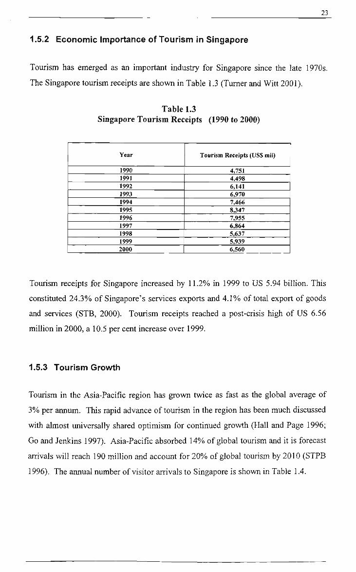
1.5.2 Economic Importance of Tourism in Singapore
Tourism has emerged as an important industry for Singapore since the late 1970s.
The Singapore tourism receipts are shown in Table 1.3 (Tumer and Witt 2001).
Table 1.3 Singapore Tourism Receipts (1990 to 2000)
Year
1990 1991 1992 1993 1994 1995 1996 1997 1998 1999 2000
Tourism Receipts (US$ mil)
4,751 4,498 6,141 6,970 7,466 8,347 7,955 6,864 5,637 5,939 6,560
Tourism receipts for Singapore increased by 11.2% in 1999 to US 5.94 billion. This
constituted 24.3% of Singapore's services exports and 4.1% of total export of goods
and services (STB, 2000). Tourism receipts reached a post-crisis high of US 6.56
million in 2000, a 10.5 per cent increase over 1999.
1.5.3 Tourism Growth
Tourism in the Asia-Pacific region has grown twice as fast as the global average of
3% per annum. This rapid advance of tourism in the region has been much discussed
with almost universally shared optimism for continued growth (Hall and Page 1996;
Go and Jenkins 1997). Asia-Pacific absorbed 14% of global tourism and it is forecast
arrivals will reach 190 million and account for 20% of global tourism by 2010 (STPB
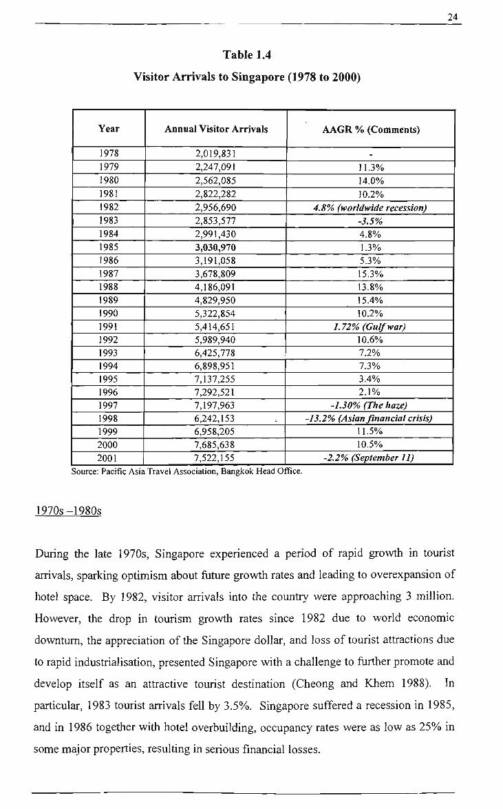
1996). The aimual number of visitor arrivals to Singapore is shovm in Table 1.4.
24
Table 1.4
Visitor Arrivals to Singapore (1978 to 2000)
Year
1978 1979 1980 1981 1982 1983 1984 1985 1986 1987 1988 1989 1990 1991 1992 1993 1994 1995 1996 1997 1998 1999 2000 2001
Annual Visitor Arrivals
2,019,831 2,247,091 2,562,085 2,822,282 2,956,690 2,853,577 2,991,430 3,030,970 3,191,058 3,678,809 4,186,091 4,829,950 5,322,854 5,414,651 5,989,940 6,425,778 6,898,951 7,137,255 7,292,521 7,197,963 6,242,153 6,958,205 7,685,638 7,522,155
AAGR % (Comments)
-
11.3% 14.0% 10.2%
4,8% (worldwide recession) -S.5% 4.8% 1.3% 5.3% 15.3% 13.8% 15.4% 10.2%
1.72% (Gulf war) 10.6% 7.2% 7.3% 3.4% 2.1%
-l.SO% (The haze) -IS.2% (Asian financial crisis)
11.5% 10.5%
-2.2% (September 11)
Source: Pacific Asia Travel Association, Bangkok Head Office.
1970s-1980s
During the late 1970s, Singapore experienced a period of rapid growth in tourist
arrivals, sparking optimism about fiiture growth rates and leading to overexpansion of
hotel space. By 1982, visitor arrivals into the country were approaching 3 million.
However, the drop in tourism growth rates since 1982 due to world economic
downturn, the appreciation of the Singapore dollar, and loss of tourist attractions due
to rapid industrialisation, presented Singapore with a challenge to further promote and
develop itself as an attractive tourist destination (Cheong and Khem 1988). In
particular, 1983 tourist arrivals fell by 3.5%. Singapore suffered a recession in 1985,
and in 1986 together with hotel overbuilding, occupancy rates were as low as 25% in
some major properties, resulting in serious financial losses.

25
The Singapore government's recognition that the poor performances of 1982 and 1983
were not due just to cyclical effects led to the development of the Tourism
Development Plan (1986-1990). The emphasis of the plan was to 'create a unique
destination combining elements of modemity with oriental mystique and cultural
heritage' (Millar 1989; Henderson 1997; Chang et al. 1996; Teo and Huang 1995; Teo
and Yeoh 1997) which resulted in a five-year restoration effort costing S$l billion.
The success of the Tourism Development Plan has resulted in an increase in visitor
arrivals into Singapore; and m 1985 tourist arrivals passed the 3 million mark.
Arrivals in 1987 totalled 3.69 million, up 15.3% over 1986. In 1988, arrivals of
foreign visitors reached a total of 4.19 million up 13.8% over 1987. By 1989, inbound
tourists increased by 15.4% to a total of 4.83 million, with hotel occupancy levels
ranging from the high 80s to mid-90s.
1990s-2000
In 1990, with an increase of 10.2% over the number of arrivals in 1989, Singapore has
a total of 5.32 million visitor arrivals. In 1991, tourism world-wide was hit by the
effects of the Persian Gulf war and Singapore's tourism industry registered only a
1.7% increase in tourist arrivals. Nevertheless, in 1992 the total number of visitor
arrivals into Singapore was on the increase again and reached 5.99 million, which
represents an increase of 10.6% over 1991. In 1994, total visitor arrivals into
Singapore reached 6.9 million up 7.3% from 1993. In 1995, the total number of
tourist arrivals exceeded 7 million.
The Southeast Asian region faced many challenges in 1997. In 1997, Singapore
annual tourist arrivals were 7.2 million, a 1.3% decline over 1996, due to the Asian
financial crisis and the environmental pollution caused by forest clearance through
burning on the two largest islands of Indonesia (Henderson 1999). When the haze
cleared in November 1997, STB launched a worldwide marketing programme.
Invitation to Blue Skies, to get both media and tour operators to come over and see
that clear skies had returned to Singapore. The financial crisis in late 1997 continued

26
through 1998, and Singapore like the rest of the countries m Southeast Asia was hit
badly resulting in a negative double-digit growth of 13.2%.
In 1999, most Asian economies began to recover from the crisis that plagued the
region the year before. At the same time, Singapore implemented a 15-month events-
packed campaign that ran from June 1999 to September 2000 called Millenia Mania
and this bold initiative resulted in visitor arrivals returning to double-digit grov^
rates of 11.5% in 1999 and 10.5% in 2000. hi 1999, total visitor arrivals mto
Singapore were 6.95 million. For 2000, total arrivals reached 7.69 million, the highest
number of visitors ever reached.
Singapore welcomed 7.52 million visitor arrivals in 2001; it's second highest in the
history of tourism, inspite of the aftermath of September 11 and the global economic
slowdown. The 7.52 million arrivals represented a drop of 2.2% over year 2000's
record 7.69 million.
27
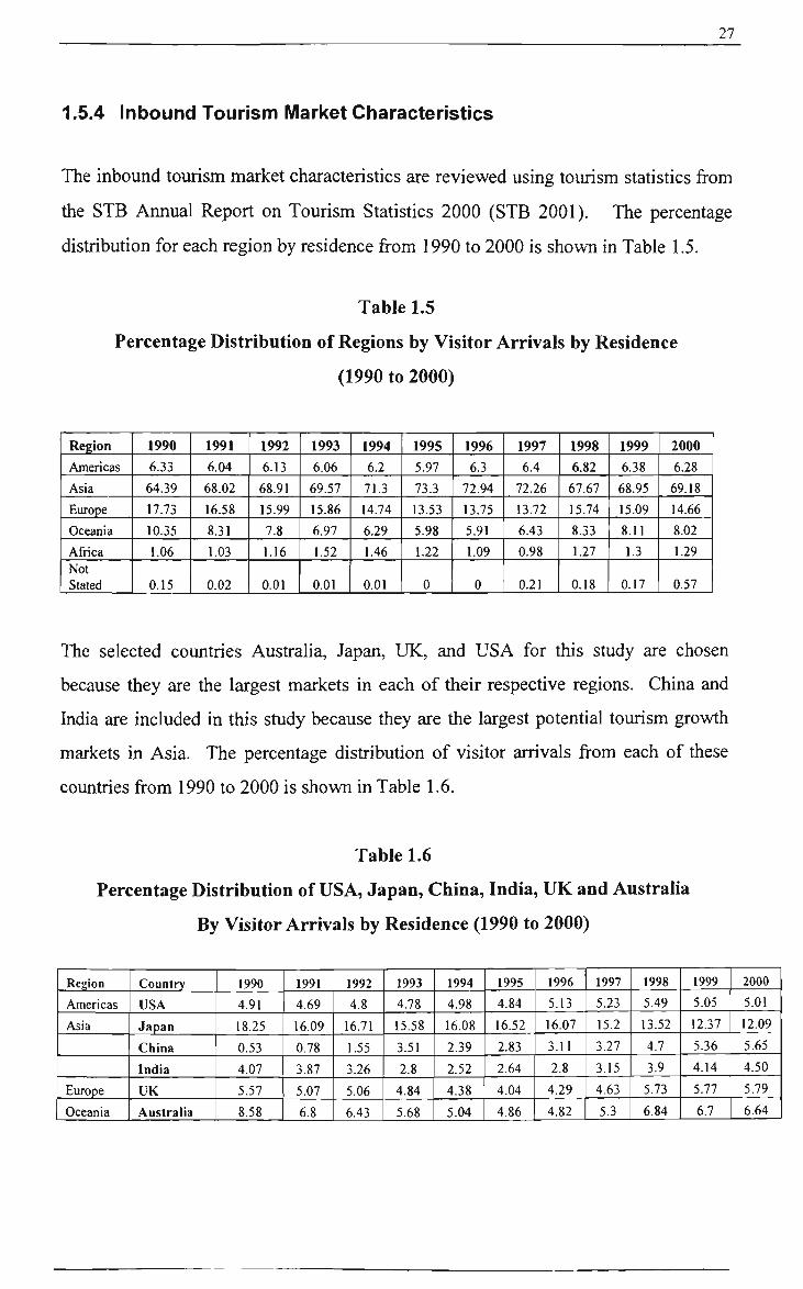
1.5.4 inbound Tourism Market Characteristics
The inbound tourism market characteristics are reviewed using tourism statistics from
the STB Annual Report on Tourism Statistics 2000 (STB 2001). The percentage
distribution for each region by residence from 1990 to 2000 is shown in Table 1.5.
Table 1.5
Percentage Distribution of Regions by Visitor Arrivals by Residence
(1990 to 2000)
Region
Americas
Asia
Europe
Oceania
Africa Not Stated
1990
6.33
64.39
17.73
10.35
1.06
0.15
1991
6.04
68.02
16.58
8.31
1.03
0.02
1992
6.13
68.91
15.99
7.8
1.16
0.01
1993
6.06
69.57
15.86
6.97
1.52
0.01
1994
6.2
71.3
14.74
6.29
1.46
0.01
1995
5.97
73.3
13.53
5.98
1.22
0
1996
6.3
72.94
13.75
5.91
1.09
0
1997
6.4
72.26
13.72
6.43
0.98
0.21
1998
6.82
67.67
15.74
8.33
1.27
0.18
1999
6.38
68.95
15.09
8.11
1.3
0.17
2000
6.28
69.18
14.66
8.02
1.29
0.57
The selected countries Australia, Japan, UK, and USA for this study are chosen
because they are the largest markets in each of their respective regions. China and
India are included in this study because they are the largest potential tourism grov^h
markets in Asia. The percentage distribution of visitor arrivals from each of these
countries from 1990 to 2000 is shovm in Table 1.6.
Table 1.6
Percentage Distribution of USA, Japan, China, India, UK and Australia
By Visitor Arrivals by Residence (1990 to 2000)
Region
Americas
Asia
Europe
Oceania
Country
USA
Japan
China
India
UK
Australia
1990
4.91
18.25
0.53
4.07
5.57
8.58
1991
4.69
16.09
0.78
3.87
5.07
6.8
1992
4.8
16.71
1.55
3.26
5.06
6.43
1993
4.78
15.58
3.51
2.8
4.84
5.68
1994
4.98
16.08
2.39
2.52
4.38
5.04
1995
4.84
16.52
2.83
2.64
4.04
4.86
1996
5.13
16.07
3.11
2.8
4.29
4.82
1997
5.23
15.2
3.27
3.15
4.63
5.3
1998
5.49
13.52
4.7
3.9
5.73
6.84
1999
5.05
12.37
5.36
4.14
5.77
6.7
2000
5.01
12.09
5.65
4.50
5.79
6.64
28
Japan accounts for about a million arrivals each year out of the seven nullion visitors
Singapore received from around the world. This makes them the number one source of
Singapore's visitor arrivals. In the year 2000, the number of visitor arrivals from
Japan was 929,895.
Austtalia has been a growth market for Singapore even during the difficult tourism
times stemming from the Asian economic crisis in 1988. The Singapore Tourism
Board opened a Marketing Representative Office in Melboume, Ausfralia in
November 1998. Within Australia, the STB has identified the state of Victoria as
having excellent potential for fiirther tourism grov^h. Victoria overtook Western
Australia in 1992 as the second largest source of visitors to Singapore from within
Ausfralia while New South Wales remained the largest source of visitors to Singapore.
Singapore's tourism presence in Australia is represented in the three biggest visitor-
generating cities and states - Sydney (NSW), Melboume (Victoria) and Perth (Westem
Austtalia). In the year 2000, the number of visitor arrivals from Austtalia was
510,347.
The United States has been consistently one of the top visitor-generating markets with
a buoyant growth rate of 9.7% in 2000 resulting in 385,585 American arrivals.
The UK is the largest market from Europe contributing 444,976 arrivals in the year
2000. European markets are significant tourism growth areas as they collectively
accounted for more than 14 per cent of visitor arrivals. For 2000, Europe as a region
demonsttated a healthy growth of 7.4%>.
China has been one of the star performers for Singapore in terms of tourist arrivals. In
1999, China overtook the United States as the sixth top visitor-generating market for
Singapore with 372,881 tourist arrivals. In 2000, the arrivals totalled 434,335.
Singapore's tourist growth in the future will increasingly depend on attracting visitors
from the new tourist generating markets of China and India.
India ranks 8 among Singapore's top visitor-generating markets. Each year,
Singapore welcomes approximately 340,000 visitors from India. Recognising the

29
potential of India as a major source of tourist arrivals, the STB has set up operations in
Mumbai in 1993, in 2001 a marketing representative was appomted in New Delhi to
service the North Asian market and in 2002 a Cheimai representative was established
to ensure that the South Indian markets will be serviced.
The visitor arrivals (from 1999 to 2001) and the forecast arrivals (from 2002 to 2004)
for USA, Japan, China, India, UK, and Ausfralia by Tumer and Witt (2001) are shovm
in Table 1.7.
Table 1.7 Forecast Arrivals of USA, Japan, China, India, UK and Australia from
(2002 to 2004)
Country USA
Japan
China India UK
Australia
1999 351,459
860,662
372,881
288,383
401,474
466,067
2000 385,585
929,895
434,335
346,356
444,976
510,347
2001 343,805
755,766
497,397
339,812
460,018
550,681
2002 342,132
897,551
487,990
350,029
427,462
562.130
2003 366,330
936,400
552,790
354,865
474.055
583,480
2004 406,730
946.570
584.110
362,260
503.560
601.800
The main purpose of visit to Singapore is classified into four categories: Holiday,
Business, Business & Pleasure, In Transit, and Others. As shown in Table 1.8,
Holiday ttavel is the dominant purpose of visit at about half of total volume. Business
ttavel also makes up a significant proportion of ttavel at 16%.
Table 1.8
Percentage Distribution of Visitor Arrivals by Purpose of Visit
PURPOSE OF VISIT
Holidav
Business
Business & Pleasure
In Transit
Others
1998
45%
16%
3%
10%
26%
1999
49%
16%
3%
10%
22%
2000
48%
16%
3%
10%
15%

30
Figure 1.1 shows the seasonality of arrivals into Singapore for the years 1999 and
2000. The peak arrival months are mostly in the second half of the year, particularly
in July and August. March, October and December are also popular months for ttavel
into Singapore (STB, 2001).
July, August and December were the peak months of fravel for visitors from Asia who
in all, accounted for over 65%o of arrivals to Singapore. Peak months of fravel for
visitors from Europe are concenfrated in the latter part of the year - in August,
October and November. The peak month of ttavel for visitors from the Americas is
usually in March. For the Oceania markets where Australia is represented, September
and October are the peak months of fravel.
Figure 1.1
Seasonality of Arrivals into Singapore for 1999 and 2000
800000
700000
600000
500000 -I
400000
300000
200000
100000
0
-1999
-2000
•8 S S. S>
^ 2 < s 5 =! o
Z Q

31
1.5.5 Tourism Development
Tourism is regarded by Singapore as an important mechanism for its economic growth
as discussed above. As such, the countiy's National Tourist Organisation (NTO)
known as the Singapore Tourist Promotion Board (STPB) was established in 1964,
with a mission to promote tourism and establish Singapore as a premier destmation
with universal appeal. The STBP changed its name to tiie Singapore Tourism Board
(STB) in 1998 and currently the STB has regional offices in Bombay, Chicago,
Frankfurt, Hong Kong, London, Los Angeles, New York, Osaka, Paris, Perth, Seoul,
Sydney, Taipei, Tokyo, Toronto and Zurich. Besides the STB, the Economic
Development Board (EDB), the national airline (Singapore Airlines), hotels, ttavel
and tour agencies, as well as the Singapore public have played an increasingly active
role in promoting tourism in the country.
Marketing efforts by the STB over the years have focused on frade and consumer
activities aimed at increasing the number of tourist arrivals, the average length of stay,
and tourist expenditure in Singapore. These tourism marketing activities or
campaigns include: (a) Intemational advertising - where major advertising campaigns
were undertaken in ASEAN, Australia, Taiwan, UK, US, Japan using both the print
and the broadcast media; (b) Consumer promotions - here the STB led sales missions
and joint promotions with airlines into countries such as Austtalia, Korea, the Middle
East counfries, and Thailand; (c) Participation in major intemational travel trade fairs -
this was conducted to raise Singapore's profile among intemational tour wholesalers
and operators; mcluding participation regularly in the ASEAN Tourism Forum (ATF),
World Travel Mart (WTM) and the Pacific Asia Travel Association (PATA) Travel
Mart; (d) Active media relations and publicity - whereby the intemational press is kept
informed of new tourism developments in Singapore through a public relations
programme consisting of seminars, publications and other relevant media education
programmes; (e) Promotion of cultural and sporting events (Weiler and Hall, 1992) -
the STB also promoted many cultural and local festivities such as the annual Chinese
Lunar New Year, Singapore's National Day celebrations, and Christmas light-up. In
promoting Singapore's reputation as an intemational sporting venue, spectacular

32
sporting events such as the Singapore Powerboat Grand Prix, Singapore Super Tennis
Tournament, Singapore World Invitational Dragon Boat Race and the Dunhill World
Cup Qualifying Round have been organised in the country by the STB.
Other than the above tourism marketing initiatives which serve to 'pull' visitors to
Singapore, the STB has adopted a forward-looking and strategic approach in
promoting Singapore as a premier tourist destination, with universal appeal, as well as
a venue and leading hub for meetings, conventions, exhibitions, incentive ttavel and
other tourism-related services. This was intended to allow Singapore to not only
capture new growth opportunities, such as those offered by the more affluent Asian
economies, but also to better meet the increased competition in the intemational
tourism market, with its limited land and labour resources.
The three major sttategies for growth implemented by the STB since its inception to
promote the country as a tourist destination are:
(1) a 1 billion "Tourism Product Development Plan" in 1986 (STPB 1986) which
called for the conservation and revitalisation of historic districts such as Chinatown,
Little India, Arab Street, Boat and Clark Quays; the upgrading of Raffles Hotel; the
development of resorts on Sentosa Island,
(2) The Strategic Plan for Growth from 1993 to 1995 to further promote tourism in
Singapore (STPB, 1993) with the objectives and sttategies listed in Table 1.9.

33
Table 1.9
Strategic Plan for Growth (1993 to 1995)
OBJECTIVES;
1. To boost tourism receipts by 10% per annum from $7.8 billion Singapore dollars in 1991 to $11.4 billion by end 1995.
2. To achieve an annual target of 25 million visitor-days by end 1995, by achieving an annual target of 6.8 million visitors by end 1995 and maintaining the 1992 average length of stay of 3.7 days.
3. To improve Singapore's position to the 6th top convention city in the world.
4. To establish Singapore as a venue with world-class special events.
5. To establish Singapore as the major cruise hub in the Asia-Pacific region.
6. To enhance the quality of the tourism experience.
STRATEGIES:
1. Increasing Singapore's share in existing key markets.
2. Forging Strategic alliances with airlines, national tourism organisations and industry members.
3. Capturing niche market segments.
4. Tapping new markets.
5. Intensifying convention promotion.
6. Developing world-class events.
7. Taking new directions in product development.
8. Improving services.
(3) the "Tourism 21 Vision" national tourism master plan launched in 1996 (STPB
1996) designed to position Singapore as a Tourism Capital, where Singapore is not
only a memorable tourist destination with plenty to see and do, but also a tourism
business centre and a tourism hub (STPB 1996). hi the words of the Tourism 21
sttategy document:

34
'Singapore is a vibrant, multicultural and progressive Asian city, located in the
heart of one of the world's most exciting and fast-grov^ng tourism and
economic regions. In other words, it embodies the essence of 'New Asia'...
After all Singapore, with its progressiveness, sophistication and unique multi
cultural Asian identity, can be said to be an expression of the modem Asian
dynamism that marks the entfre region - the island is a place where ttadition
and modemity. East and West meet and intermingle comfortably (p. 25).'
According to this strategy, as a Tourist Destination, Singapore must be a centte of
attraction in its own right. As a Tourism Business Cenfre, Singapore must be in a
position to attract the very best tourism businesses to take a stake in Singapore. As a
Tourism Hub, Singapore must assume the position of a switching node; a springboard
for visitors venturing into the region and vice versa as well as a headquarter for
tourism-related businesses in the region. Broadly, the six distinctive sttategic thmsts
of Tourism 21 are as follows:
(1) Redefine tourism with new tourism products such as business centte, hub
and New Asia,
(2) Reformulate products to be sophisticated to cater to demanding tourists
with thematic developments, hardware and software hamessed in technology,
(3) Develop tourism as an Industry involving a cluster of industries (Porter
1990) with a creative, productive and service-oriented workforce,
(4) Configure new tourism space in terms of Singapore's own facilities and
regional resort and selected destinations which are imlimited,
(5) Partnering for success involves public, private sectors on a win-win
concept, and,
(6) Championing tourism with STPB being renamed to STB with wider
powers and capabilities.
In conjunction with these thmsts, the image of Singapore as a vibrant cultural scene,
cosmopolitan and dynamic is projected using the New Asia-Singapore Brand
inttoduced in 1996. However, Henderson (2000) found in her survey that tiiere is still
a lack of awareness amongst both its tourists and locals of the New Asia-Singapore
35
brand and concluded that devising and implementing meaningfiil brands remains a
challenge for destination marketers. Kotler et al. (1996), Ward (1998) and Buhalis
(2000) highlighted that destination marketing has become increasingly important. In
addition, the creation of the right destination image through branding is a challenging
task (Echtner and Ritchie 1991; Chon 1992; Waitt 1996; Morgan and Pritchard 1998).
A second aspect of the Tourism 21 master plan comes under the slogan "Tourism
Unlimited" and the thmst is to develop and expand Singapore's role as a business and
investment centre for the Asia Pacific Region. STB (1996) highlighted that with the
successful implementation of the Tourism 21 vision, Singapore auns by the year 2005
to welcome its 10 millionth visitor and to receive S$16 billion in tourism receipts.
This seems achievable judging by the successes that Singapore has received in recent
times. In 2002, Singapore was voted the Favourite Business City in the world in an
aimual readership poll conducted by Business Traveller Asia Pacific (BTAP).
Singapore was ahead of more than 30 cities to take the top spot in the Favourite
Business City category with Hong Kong in second place and London, third.
Singapore also swept the polls in other categories. Singapore Airlines won six awards
including the Best Airline in the World, and the Best Asian Airline. Changi Airport
won for the Best Airport and Best Duty Free categories. In 2001, thousands of
travellers in Asia and Europe have also voted for Singapore as their Best Business
Destination. This was the imanimous result of three separate readership polls
conducted by Time Magazine, Business Traveller Asia Pacific (BTAP) and Business
Traveller UK (BTUK). For the year 2001, about 19% of total visitor arrivals to
Singapore were business travellers. Also in April 2001, Singapore was awarded the
Destination of the Year. This award was presented at the end of the annual PATA
Travel Mart. In March 2001, at the ITB 2001 (Intemationale Tourismus Borse), a
major ttavel trade event held annually in Berlin, the Singapore Tourism Board (STB)
was awarded the Best Marketing Effort recognising STB has succeeded in putting
across its tourism products and services in a clear, creative and consistent manner.
For a third year miming, the Singapore Tourism Board has been named the "Best
National Tourist Organisation" at the prestigious 1998 Travel Awards; in 1998 STB
also won the same award organised by the Miller Freeman Group.

36
It can be seen that tourism development initiatives by the STB over the years have
resulted in tourism growth and an economic contribution to Singapore. The tourism
strategies for growth developed and implemented by the STB indicate a high level of
commitment by the STB and its management to sttategic planning. Key sttategic
frameworks for tourism are discussed by Porter (1980), Gilberts (1990), Poon (1993),
and Tribe (1997). The need and the effectiveness of the strategy development and
implementation procedures adopted by the NTO are highlighted by Athiyaman and
Robertson (1995) and Soteriou and Roberts (1998). Ooi (2002) concluded that STB
in additional to taking initiatives, it's success and tourism plans are well supported by
the government policies and valuable resources and this has contributed to STB
success.
In summary, the factors that have contributed in the success and grov^ of
Singapore's' tourism industry are as follows:
a) High level investment by government and the private sector, which resulted in good transportation, telecommunications and financial infrastmcture.
b) The variety of admission-charging tourist atttactions and public places of interest.
c) The availability of a vside range of excellent value-for-money accommodation facilities to suit the needs of various types of visitors.
d) The social and political stability of a modem city.
e) The positive and welcoming attitudes of a well-ttained English speaking workforce serving the tourism industry created by both its culture and education and training system.
f) The accessibility of Singapore especially by air, land and sea due to its open-skies policy and its strategic location at the 'crossroads of the world' acting as a regional hub and gateway to the Asia- Pacific region. It is also an important stopover point for long-haul travellers. The opening of Changi Intemational Airport Terminal 1 in 1981 and Terminal 2 in 1990 has provided greater accessibility to intemational visitors.
g) A clean, green and safe city with an all-year round warm and pleasant ttopical climate.

37
h) An excellent venue for social and business meetings and functions because of its clean, safe and efficient reputation internationally.
i) A shopping and food paradise. Singapore offers good shopping facilities and good service with shoppers being protected by consumer protection and licensing policies.
j) A unique blend of Asian traditions and culture with Asian visitors feeling at home and Westerners intrigued by its multicultural society.
k) The high level of awareness of Singapore created by government participation in trade missions, sales missions and promotional campaigns in selling Singapore as a tourist destination.
1) Rapid economic growth of the Pacific Rim region leading to a corresponding increase in personal disposable incomes and consumerism.
The growing importance of tourism and growing maturity of Singapore as a tourist
destination pose a great challenge to Singapore. Given its small size and lack of
natural resources and attractions, it will be increasingly difficult for Singapore to
sustain high levels of growth in visitor arrivals and tourism receipts or eamings. In
addition, as the regional countries develop and open their markets, Singapore will also
have to contend with intensifying competition. The question that is now raised is
whether it is possible to use practical time-series models to further advance the
planning of tourism development in Singapore.
38
CHAPTER 2 LITERATURE REVIEW
Introduction
This chapter reviews the various qualitative and quantitative forecasting methods that
have been applied to tourism demand forecasting. Section 1 reviews qualitative
forecasting methods that include surveys, jury of executive opmion and the Delphi
method. In Section 2 quantitative forecasting methods are reviewed and are
subdivided into causal and time-series methods. Causal methods include regression
analysis and error correction models. The quantitative time series methods reviewed
include the naive method, moving average, exponential smoothing, Box-Jenkins,
stmctural time-series models, and Neural Network models.
Tourism demand modelling and forecasting have been well discussed by Song and
Witt (2000), and reviews of empirical research have been done by Bar On (1979),
Uysal and Crompton (1985), Sheldon and Turgut (1985), Calantone et al. (1987), Witt
(1989a, 1989b), Crouch and Shaw (1990), Crouch et al. (1992), Crouch (1994), Witt
(1994), Witt and Witt (1995), Lim (1997), Song et al. (1999). Tourism forecasting
methods can be divided into (a) qualitative, and (b) quantitative methods which in ttim
can be subdivided into non-causal quantitative techniques and causal quantitative
techniques.
Regardless of the type of forecasting method used, the usefulness of any tourism
demand forecasting model is really determined by the accuracy of the tourism
forecasts that it can generate, as measured by comparison to actual tourism flows
(Mahmoud 1984).
Frechtiing (1996, 2001) provides a usefiil distinction between a forecasting method
and a forecasting model as follows:

39
"A forecasting method is simply a systematic way of organising information
from the past to infer the occurrence of an event in the future. 'Systematic'
means follovdng a distinct set of procedures in a prescribed sequence .
A forecasting model is one expression of a forecasting method. More
specifically, it is a simplified representation of reality, comprising of a set of
relationships, historical information on these relationships, and procedures to
project these relationships into the future." (1996, p. 19).
Figure 2.1 shows the list of forecasting methods that are reviewed in this chapter
under the qualitative and quantitative classification headings.
Figure 2.1
Types of forecasting methods
A. Qualitative
1.
2.
3.
Jury of executive opinion
Delphi method
Surveys
B. Quantitative
1.
2.
Causal methods
a. Regression analysis
b. Error Correction Model
c. Multivariate Structural Model
Time-series methods
a. Na'ive
b. Simple Moving Average
c. Decomposition
d. Exponential smoothing
e. Box-Jenkins Approach
f. Basic Structural Model
g. Neural Networks
40
2.1 Qualitative Forecasting Methods
Qualitative forecasting methods, also called 'judgemental methods' or 'subjective
forecasting' rely on managerial or expert judgement without using specific models.
Therefore, different individuals using the same qualitative method may arrive at
v^dely different forecasts. However, these methods are useful when there is a lack of
historical data or when the historical data are not reliable predictors of the future.
2.1.1 Jury of Executive Opinion
In this approach, forecasts are made by a group of executives on the basis of
experience, hunches, or facts about the situation. This approach is aimed at generating
as much debate and interchange of ideas as possible in order to reach a consensus on
the forecast. The advantages of this technique are: (1) simplicity, (2) it does not
require much historical data, and (3) the most experienced executives can be brought
together to make the forecasts. The disadvantages include: (1) it requires costly
executive time, (2) the lack of consistency in the generated forecasts, (3) the
'bandwagon' effect where participants are reluctant to state views at odds with a
developing consensus, and (4) the most forceful or senior executive's opinion might
carry the most weight, which might lead to a poor forecast.
Example Application
Moutinho and Witt (1995) adopted a consensus approach method that permits full
discussion among the experts, in forecasting and ranking the importance and impact of
possible future developments in science and technology affecting tourism. The results
show that the experts expect advances in science and technology to have major
impacts on tourism development during the period up to 2030. This approach was
useful as it supports the clarification of reasoning for proposed developments.

41
2.1.2 Delphi Method
The Delphi metiiod (Brown 1968; Robinson 1979; Taylor and Judd 1989; Rowe et al.
1991; Moeller and Shafer 1994; Rowe and Wright 1999) which was developed by the
RAND Corporation, has been widely applied to tourism forecasting.
The Delphi method is conducted through a sequence of steps. On the first round, each
participant of the panel provides a written response to the questions asked. Responses
are fed back to the panel, and each participant is then asked to reconsider his or her
previous answers and to respond to the questions again. This procedure is repeated
for four to six rounds until sufficient convergence is achieved from the collective
knowledge of the participants (Robinson 1979). Thus, the estimates from the last
round are used as the forecasts. The Delphi method has attracted the most attention of
the several qualitative methods because all estimates from the panel of experts are
treated anonymously. Anonymity eliminates the influence of the supposed greatest
authority, as well as the 'bandwagon or herd effect' that is so common in the 'jury of
executive' opinion method (Frechtling 1996). However, the feedback process of the
Delphi method is criticised as having a tendency to force convergence toward the
group centre, which has sometimes been referred to as 'pool ignorance' (Schroeder
1982). This method also requires a substantial amount of time from beginning to the
end, resulting in panel attrition. Seely et al. (1980) highlighted that the most
important potential weakness of the Delphi method is not asking pertinent questions,
while Taylor and Judd (1989) consider the most important step is choosing the
respondents.
Example Applications
Kaynak and Macaulay (1984) use the Delphi technique to gather data on tourism
research, on future impacts of tourism and to sttengthen a regional data base, all of
which are intended to act as an effective policy-making tool in solving management
and planning problems in the tourism and hospitality industry of Nova Scotia, Canada

42
to the year 2000. The questions were posed to 150 judges, and after two rounds, 44
completed questionnafres were retumed.
Liu (1988) used the Delphi forecasting technique to forecast tourism to Hawaii,
particularly Oahu, by the year 2000. Local experts and travel agents were questioned
on visitor arrivals and percentage of domestic arrivals to Hawaii, market share, visitor-
to-resident ratio, maximum visitor accommodation and desirable growth rates, and
probable scenarios for Oahu tourism. The results show few significant differences in
responses among the groups, and confirmed expectations about convergence and
consistency of managerial responses with statistical projections and existing trends.
Yong, Keng and Leng (1989) used the Delphi method to project the future of
Singapore's tourism industry from 2 different panels, one consisting of people from
the local tourist industry and the other consisting of an intemational group of business
executives. The conclusions highlighted (a) positive future ttends that include: 1.
increased purchasing power for leisure and ttavel services for individuals from
developed coimtries, 2. better access to ttavel information, 3. fewer consttaints for
cross-border ttavel movements, and 4. higher pressure for regional collaboration in
tourism-related activities; and (b) negative trends which include the imposition of
more stringent exit taxes and a decrease in business ttavellers.
Miller (2001) presented the results of a two round Delphi study conducted into expert
opinion on the development of indicators for sustainable tourism. The results of this
dephi survey show considerable disagreement over 'sustainability' and where the
borders of the concept exist.
2.1.3 Surveys
The two survey approaches in qualitative forecasting are: (1) national or regional
surveys of tour operators, travel agencies, and airlines, and (2) surveys of visitors or
potential visitors as to whether they anticipate a frip to the tourism destination areas.
The analysis of these surveys often provides valuable insights into emerging tourism

43
ttends in the short to medium term. However, the survey approach is time consuming
and expensive and the conclusions dravm can be biased or incorrect due to (a)
sampling errors, (b) non-response errors, and (c) response errors.
In summary, qualitative forecasting methods have more value applied to medium- and
long-range forecasting, and are considered to be less rigorous than the quantitative
forecasting methods. However, they are appropriate where data is insufficient or
unreliable for the application of quantitative forecasting methods (Archer 1987; Var
and Lee 1993). Sheldon and Turgut (1985) in their review of empirical research on
tourism forecasting concluded expert-opinion methods are useful when data are
unavailable. Another key advantage of qualitative methods is that they do not require
high-level statistical skills to conduct forecasting. Sanders and Manrodt (1994) found
that companies still relied heavily on judgmental methods, even though the knowledge
of quantitative methods seemed to be improving. In another study by Frank and
McCollough (1992) it was found that judgement (82% of the respondents) was most
widely used followed by the quantitative methods such as moving averages and
exponential smoothing to obtain forecasts.

44
2.2 Quantitative Forecasting Methods
The basic divisions of the quantitative forecasting methods are causal and time-series
forecasting.
2.2.1 Causal Methods
2.2.1.1 Regression analysis
The linear regression method is one of the major approaches to causal modelling in
tourism demand forecasting (Frechtling 1996). The general form is given as:
Yt = a + Pi xi + P2 X2 + p3 X3 + p„ Xn + e
where:
Y = the dependent of forecast variable,
a = intercept constant,
P = slope coefficients,
x = independent, or explanatory, variables,
n = number of explanatory (independent) variable,
e = error term.
The regression line is a linear time ttend regression of the data series that minimises
the sum of the squared vertical departures (i.e. residuals) of the data from the
regression line; hence the technique is called 'least squares regression' or 'ordinary
least squares regression' (OLS) (Greene 1997).
Regression models include simple regression and multiple regression. In simple
regression, there is only one explanatory variable affecting the dependent or forecast
variable. Mathematically, it is expressed as:
Yt = po + Pi x,+ et
where:
Yt = dependent or forecast variable,
45
Po = intercept constant estimated by least squares regression.
Pi = slope coefficient estimated by least squares regression,
x t = explanatory (independent) variable,
Ct = error term.
With simple regression, a 'misspecification' problem can occur and this can be due to
one or more relevant explanatory variables being excluded from the simple regression
equation. As such, the multiple (or 'multivariate') regression model with two or more
explanatory variables is more commonly used and is expressed as:
Y = Po + Pi bi + P2 X2 + Pn Xn + e
where:
Y = dependent or forecast variable,
Po = intercept constant estimated by least squares regression.
Pi = slope coefficient estimated by least squares regression,
X = explanatory (independent) variables,
n = number of explanatory variables,
e = error term.
The possible explanatory variables or determinants of tourism demand (Moriey 1991
1996; Witt and Witt 1992; Frechtiing 1996; Lim 1999; Song and Witt 2000) include
the following:
(a) Population
- It is expected that the level of inbound tourists into the destination country
depends upon the population of the tourist generating countries. Therefore,
population can be used as an explanatory variable. Although, excluding the
population variable is not likely to affect the model significantly, as population
changes in the tourist generating countries are normally small over the short to
medium term. The main argument for not having population as a separate
variable is that it may cause multicoUinearity problems. Population can also
act as a surrogate variable for time change reflecting tourism growih rates that

46
are common over time but not 'caused' by population change. In this way, a
population variable can act as 'spurious' independent variable,
(b) Income
- The real per capita income of visitors from the tourist generating country is
normally used as an explanatory variable (Crouch 1992). Income is an
important explanatory variable in nearly all forecasting demand studies and is
a direct and current determinant of the capacity of individuals within a given
market to afford travel,
(c) Expenditure on the tour or price
- The expenditure on the tour can be included as an explanatory variable in
regression analysis; and it consists of two components: (i) ttavel cost to the
destination, and (ii) cost of living for the tourist in the destmation (Martin and
Witt 1987).
Travel costs could be air fares between the origin and destination, ferry fares,
and/or pettol cost (based on the distances travelled) for surface ttavel.
However, ttavel cost as a demand determinant is often excluded from the
models due to potential multicoUinearity problems, and the difficulty in
obtaining this data (Uysal and Crompton 1984).
The consumer price index (CPI) in a country is usually taken as a reasonable
proxy for the cost of living for the tourist in the destination. As Kliman (1981)
highlighted where 'the data do not represent the underlying variables as
accurately as one would like ... there are some instances in which only rough
approximations to the theoretically correct constmcts are possible'. Gray
(1966) commented that 'prices are seldom completely known in advance by
ttavellers so that the price level foreseen by the potential traveller will depend
predominantly upon the rate of exchange of his domestic and [the destination
currency]'. Thus a reasonable proxy for the cost of tourism is the exchange
rate adjusted consumer price index. Using exchange rate on its ovm is not an
acceptable proxy as consumers could be misled; as a favourable exchange rate
47
could be counterbalanced by a relatively high inflation rate. For all-inclusive
tours, both the fravel cost element and the tourists' cost of living element are
often added into a single cost variable as a determinant (Witt 1983).
(d) Substitute prices
- Prices of substitutes may be important determinants of demand in causal
models. Gray (1966, p.86) highlighted that: '...there is a high elasticity of
tourism demand substitution among countries so that higher than expected
prices in one country may result in a change of destination rather than a
decision to forgo overseas travel'. Thus both the tourists' fravel costs (White
1985; Martin and Witt 1988a; Rosenwseig 1988) and tourists' living costs at
the destination are just as likely to cause substitution possibilities thereby
influencing the demand for tourism to a destination. From the review studies,
it is found that substitute tourists' living costs are used more often than
substitute ttavel costs (Gray 1966; Kliman 1981; Papadopoulous and Witt
1985).
(e) Dummy variables
- These are included in the regression model to allow for the effect of 'one-off
events. These variables take the value 1 when the event occurs and 0
otherwise. Thus the impact of events such as the oil crises and mega-events
such as the Olympic Games can be incorporated as dummy variables (Witt and
Martin 1987c; Smeral et al. 1992). Dummy variables can also be used to
accommodate the effects of seasonality (Chadee and Mieczkowski 1987) when
quarterly data are used in tourism model estimation. Additionally, for multi-
destination models, dummy variables are used to represent destination
'attractiveness' (Witt 1980a) with the assumption that the relative attractiveness
of the destinations remains the same over the time period considered. In
reality this is not necessarily tme or possible.
(f) Trend
- A ttend variable representing the steady change in the popularity of a
destination country over the time period considered can be included in the

48
tourism demand model. Therefore this variable captures time-dependent
effects of all the other independent determinants that have not been explicitiy
incorporated in the model, such as demographic changes in the origins.
(g) Marketing expenditure
- The marketing expenditure of national tourist organisations, used specifically
for the promotion of the country as a tourist destination, is expected to have a
significant effect on the level of intemational tourism demand. Promotional
activities that include media advertising and public relations are often used to
create interest and persuade potential visitors to ttavel to the particular country.
However, there are problems associated with: (i) obtaining the relevant data,
(ii) defining the relationship of this particular variable due to the distribution
effect of advertising over time (that is, the advertising in a given period is
likely to influence not only the immediate period but also subsequent periods),
and (iii) assessing the effectiveness of a given level of advertising expenditure
on tourism demand, as it often varies across media. Empirical studies that
have included some form of marketing variable, in their tourism demand
models include those by Barry and O'Hagan (1972), Uysal and Crompton
(1984), O'Hagan and Harrison (1984) and Papadopoulous and Witt (1985).
(h) Lagged dependent variable
- A lagged dependent variable can be included in the tourism demand function
to bring in the effect of (a) habit persistence, that is, a visitor would tend to
retum to a particular destination in fiiture if the visitor likes the place; there is
less uncertainty associated v^th touring that destination again as compared to
ttavelling to a new and foreign environment, and (b) supply consttaints (Smith
and Toms 1967; Witt and Martin 1987a).
Other than determining the causal variables, it is the responsibility of the forecaster to
define the matiiematical relationship or functional form (linear, nonlinear, additive, or
multiplicative) of the tourism demand model. The log-linear form has been more
popular due to its association with elasticities and superior empirical results compared
49
with the corresponding linear fimctional form (Artus 1970; Barry and O'Hagan 1972;
Uysal and Crompton 1984; Witt 1987a; Johnson and Ashworth 1990; Crouch 1994).
Other functional forms include the semi-log (O'Hagan and Harrison 1984; White
1985), the Probit and Logit models (Witt, 1983), and a non-linear, diffusion form
(Moriey 1998, 2000). Moriey (1991) highlighted a wrong functional form can have a
significant impact on the model estimated. Song and Witt (1995) highlighted that
'For tourism demand forecasters, correctly identifying the determinants of tourism
demand and appropriately specifying the tourism demand models are cmcial for the
generation of accurate forecasts of future tourism demand.'
In regression models, once this estimated mathematical relationship and the
explanatory variables are established, forecasts into the future are obtained. As
mentioned, the forecasting model parameter estimates are generated using the ordinary
least squares (OLS) estimation method (Moriey 1997); sometimes this method is
augmented by the Cochrane-Orcutt procedure if autocorrelated residuals are identified.
The OLS estimator for the parameter of an explanatory variable in a regression model
is a constant and the best linear unbiased estimator of the parameter if the error term,
e, satisfies the following basic assumptions:
1. Zero mean: E(e) = 0 . 1 1
2. Homoskedasticity or constant variance: E(e ) = CTg . 3. Nonautocorrelation: E(etek) = 0 for t ^ k .
4. Uncorrelated with explanatory variable Xt : E(xt Ct) = 0 .
The sttength of the relationship between the forecast (dependent variable) and the
causal explanatory variables is calculated using the coefficient of determination, R .
That is, R , is the proportion of the total variation in the observed values of the
dependent variable that is explained by the overall regression model. Values of R
close to 1 indicate a close agreement between the model and data, while values close
to 0 indicate a poor fit. To avoid the trap of only trying to find a model that
maximises R , a 'good' regression model is selected based upon the following
properties (Famum and Stanton 1989):
50
(1) it should be a simple model with a reasonable number of predictor
variables,
(2) it should have a statistically significant overall F-value, showing tiie
usefulness of the entire set of predictor variables,
(3) it should have statistically significant partial t-values for each of the
predictor variables. The partial-t values test whether the variable adds
significantiy to a model already containing the remaining predictor variables,
(4) a high R value should be obtained from the model.
It has been recognised that certain problems can arise using the regression forecasting
methods above: (a) it requires considerable user understanding in order to determine
the causal stmcture, (b) it is generally more expensive and more complex through the
inclusion of more explanatory variables, (c) more importantly, the dependence on
predictor variables which are often themselves estimated or imavailable at the point of
estimation, (d) the accuracy of the forecasts is highly affected and dependent on the
accuracy of the predictor variables, and, (e) low levels of achieved accuracy despite
high R measures often occur. Generally, 'satisfactory' or 'acceptable' causal tourism
demand models can be identified using criteria based on: (i) Durbin-Watson (DW)
statistic - indicating no autocorrelation at the 5% significance level, (ii) 'correct' signs
for the predictor variable coefficients, and (iii) F statistic - indicating that the equation
is significantly different from zero at the 5% level. The 'best estimated' model is then
identified from these acceptable models by comparing their coefficient of
determination (R ) and the statistical significance of the coefficients using t statistics.
However, this assessment can be misleading as the appropriateness of the independent
variables in the estimated model may change over the forecast time period, and this
can lead to a decline in the accuracy of the model. One test for the stability of the
forecasting model is the Chow predictive failure test described in Song and Witt
(2000) and Frechtiing (2001). As Witt and Witt (1990) highlighted: 'Conditions such
as a high goodness of fit and a large proportion of statistically significant coefficients
do not appear to be sufficient to ensure a high level of forecast accuracy'.
In addition, with the regression forecasting technique, care is needed to deal with the
following problems:
51
(a) Heteroscedasticity; which implies that the residuals do not maintain
constant variance throughout the time series.
(b) MulticoUinearity; which refers to the correlation among explanatory
variables (Fujii and Mak 1980). This was 'the most common
methodological problem encountered' as highlighted by Crouch (1994)
in his review of 85 tourism demand forecasting models.
(c) Autocorrelation of the error terms or residuals that can lead to an
inappropriate model (Cook and Weisberg 1982). In regression models,
error terms or residuals are assumed to be an independent white noise
sequence with zero mean which has constant variance, independence,
and normality assumptions. The presence of autocorrelated residuals
may be detected by using residual plots and the Durbin-Watson statistic
d test (Durbin and Watson 1951). Values close to 0 indicate positive
autocorrelation, values close to 4 indicate negative correlation, and
values close to 2 indicate independent error terms.
(d) Spurious relationships, which occur when statistical evidence points to
the existence of a relationship between variables where, in fact, none
exists and are another serious problem found in regression models
(Granger and Newbold 1974; Skene 1995; Morris et al. 1995). In
particular, many tourism demand variables are non-stationary and using
the ttaditional regression model and obtaining a high R can lead to a
false conclusion that these variables are actually related when they are
not. This problem of a spurious relationship has led to the use of co-
integration analysis designed to overcome the problems of stationarity
and these issues are discussed further below.
Moriey (1991) highlighted that it is unlikely "that the widespread use of multiple
regression for estimating tourism demand functions will diminish, given its widely
perceived advantages over other ways of forecasting demand". However, he
highlighted that while problems of heteroscedasticity, multicoUinearity, and
autocorrelation are well recognized by modelers, questions of model specification are
less widely understood. Misspecification of the multiple regression model, such as

52
failure to include an important explanatory variable or a wrong functional form, can
have significant impacts on the model estimated. He concluded that more complex or
general functional forms yield better models than more simple functions, such as the
commonly used log-linear model.
Example Applications
Choy (1984) examines the accuracy and efficiency of forecasting techniques by
applying time series regression to forecasting visitor arrivals. Past studies have shovm
that simpler time series techniques perform as well or better than complex forecastmg
models. An assessment of visitor forecasts developed at regional, destination and
individual market levels suggests that time series regression performs well in
producing annual forecasts of visitors which can serve as a baseline for evaluating the
net benefits, if any, from applying more complex techniques. He highlighted that
tourism managers should appreciate the usefulness of simpler formal methods in
developing forecasts of visitors.
Witt and Martin (1987b) explored the inclusion of marketing variables in intemational
tourism demand models, as National Tourist Organizations often spend considerable
sums in foreign countries on promoting the particular country as a tourist destination.
However, marketing activity is seldom incorporated as an explanatory variable in
models of the demand for intemational tourism. It was highlighted where marketing is
used to explain intemational tourism demand, caution must be exercised in
interpreting the empirical results; poor results cannot be used to reach sensible
conclusions, and when good results are obtained the full implications of the estimated
coefficients need to be explored.
Smeral, Witt and Witt (1992) specified a complete system of econometric demand
equations to generate forecasts of tourism imports and exports for various major
geographical areas. The forecasts are presented for the period 1991 to 2000 under
three alternative assumptions: (1) there is no change in the extemal environment
(baseline scenario), (2) the completion of the single intemal market of the European
Community takes place, and (3) the liberalization and general creation of market
. 53_
economies in Eastem Europe. A comparison of the latter two scenarios with the
baseline scenario was made to explore the effects of these changes on the tourism
demand forecasts.
Crouch et al.'s (1992) study estimated the impact of the intemational marketing
activities of the Austtalian Tourist Commission (ATC) on the number of tourist
arrivals into Austtalia. Multivariate regression analysis was employed in order to
estimate the elasticities of demand from five origin countries (USA, Japan, New
Zealand, UK and FR Germany) using a set of determinants that include both total
ATC marketmg expenditure and advertising-only expenditure. The results suggested
that intemational marketing activities of the ATC have a significant role in
influencing inbound tourism to Australia from these countries. The best estimates of
the marketing elasticities for the USA, Japan, New Zealand, the UK and FR Germany
were +0.11, +0.20, +0.25, +0.14, and +0.23 respectively.
Chan (1993) employed a regression model that comprises a linear term in time and a
sine function in time to fit the monthly total tourist arrival data in Singapore.
Because of the seasonal fluctuation in the data, deseasonalised data was used in fitting
the model. This regression model was compared with the naive 1 model, naive 2
model, a simple linear regression time series model, and an ARIMA (2,1,2) model
using the mean absolute percentage errors (MAPEs) generated in forecasting the
monthly tourist arrivals from January 1989 to July 1990. The result indicated that the
sine wave time series regression model was the best forecasting model with a MAPE
of 2.56%.
Crouch (1994), through his survey of the practices of past empirical studies of
intemational tourism demand, highlighted the methodologies employed vary in a
number of ways. Ordinary least-squares (OLS) multivariable regression analysis was
identified as the most widely used approach. In terms of tiie functional form of the
model, it was found that there appears to be almost universal agreement that the
multiplicative (i.e., log-linear) form is superior to the additive (i.e., linear) form. In
addition, it was found that tiie most common metiiodological problem encountered has
been the difficulty of separating the effect of certain determinants as a result of

54
multicoUinearity. He concluded the selection of the most suitable approach will
depend upon the circumstances and objectives of the study being planned, and it
would be wrong to blindly adopt any one approach without first judging its limitations
and assumptions.
Witt and Witt (1995) provided a review of empirical research of forecasting tourism
demand studies and found that the vast majority of such studies are concemed with
econometric modelling/forecasting with emphasis placed on empirical comparisons of
the accuracy of tourism forecasts generated by different techniques. They highlighted
considerable scope exists for improving the model specification techniques employed
in econometric forecasting (Allen and Fildes 2001) of tourism demand.
Qu and Lam's (1997) study was to determine what exogenous variables best explained
the ttavel demand for Mainland Chinese tourists to Hong Kong. A 12 year (1984-
1995) annual time series data set of 'Mainland Chinese tourist arrivals', 'China
disposable income per capita', 'consumer price indices in Hong Kong and China' and
'exchange rates' was used to develop a ttavel demand model. Seven exogenous
variables were selected for the model. The OLS multiple regression analysis was
performed to identify the 'best' subset of seven exogenous variables to determine the
demand model. The results showed that ttavel demand for Mainland Chinese tourists
to Hong Kong could be explained by 'disposable income per capita' and 'relaxation of
visa requirements'.
Aki (1998) examined the relationship between tourism demand for Turkey and
national income of the tourist generating country at constant prices, and relative prices
(prices in the host country divided by prices in the tourist generating country) using a
double-logarithmic fimctional form of the regression model. The results indicated a
positive relationship between tourist arrivals and national income for the tourist
generating countries, and a negative relationship between tourist arrivals and relative
prices.
Kulendran and Wilson (2000) attempted to identify those economic variables that are
most important in influencing business ttips to Austtalia from four of Australia's most

55
important ttavel and ttade partners. They found that the importance of the economic
variables varies from country to country, although overall openness to ttade and origin
country real income are important variables explaining business fravel to Austtalia
from these origin countries.
2.2.1.2 Error Correction Models
In a stationary time series the mean, variance and covariance will not change through
time. If the time series analysed is non-stationary, using a regression model with the
assumption of stationarity would give misleading results (the spurious regression
problem). For a non-stationary time series, the ordinary least squares coefficients do
not generally follow a normal distribution and the validity of tests such as the t test are
in doubt. Moreover, the F test for the overall contribution of the independent
variables is also invalid, as the F distribution does not hold. Nelson and Plosser (1982)
indeed found non-stationarity in many macroeconomic variables and these would lead
to spurious inferences when using them in formulating the models.
The cointegration technique developed by Engle and Granger (1987), together with
the error correction mechanism is the proposed solution to the spurious regression
problem when non-stationary time series are used in tourism demand modelling.
Song and Witt (2001) provided a detailed description on cointegration and ECM. In
summary, the use of cointegration raises the level of complexity in tourism demand
modelling with the need to: (1) identify the order of integration using tests such as the
Dickey and Fuller (DF) and Augmented Dickey-Fuller (ADF) tests (Dickey and
Fuller, 1981), and the Hylleberg, Engle, Granger and Yoo (HEGY) (1990) test; (2) test
for cointegration, (3) estimate the ECM using either the Engle-Granger two stage, the
Wickens-Breusch one-stage (Wickens and Breusch 1988) or the ADLM (Pesaran and
Shin 1995) procedures.
In terms of forecasting accuracy performance, ECMs have been shovm to perform
well more for medium and long forecast horizons by Engle and Yoo (1987) and
Hofman and Rasche (1996). Clements and Hendry (1995) showed that the sample
^___ 56_
size and representation of data are of great importance for forecasting performance
improvement. Applications of cointegration and ECM for tourism forecasting include
Kulendran (1996), Kulendran and King (1997), Latiiiras and Siriopoulous (1998),
Kim and Song (1998), Song et al. (2000), Kulendran and Witt (2001).
Example Applications
Lathiras and Siriopoulous (1988) was the first study to forecast demand for tourism
using a cointegrated approach. In the study, tourist arrivals to Greece from six
important generating countries were considered: the UK, Germany, Italy, France, the
USA, and Holland using a total of 36 years' data from 1960 to 1995. As the economic
determinants of tourism demand were integrated to the order of one, cointegration
analysis and ECM methodology were applied to estimate the short- and long-run
demand for tourism. They concluded that although past empirical studies do not
indicate clearly that ECMs outperform regression models in forecasting, their results
have shown that the estimated short-run demand models have good forecasting power.
Kulendran and King (1997) compared a range of forecasting models in the context of
predicting quarterly tourist flows into Austtalia from the major tourist markets of
USA, Japan, UK and New Zealand. Models considered included the error-correction
model, the autoregressive model, the autoregressive integrated moving average model,
the basic structural model and a regression based time series model. They found that
the forecast horizon and country of origin are important parameters for the forecasting
performance of various time series models.
Song et al. (2000) explored UK demand for outbound tourism to 12 destinations using
error correction models. Ex post forecasts over a period of 6 years are generated from
the ECM models and the results compared with those of a naive model, an AR(1)
model, an ARMA (p,q) model, and a VAR model. The forecasting performance
criteria show that the ECM model has the best overall forecasting performance for UK
outbound tourism, although the improvement is not statistically significant at 5%.
57
2.2.1.3 Multivariate Structural Model
The single multivariate regression model assumes the only causality is from each
explanatory variable to the forecasting variable, and does not capture feedback and
cross-dependencies that might be present estimating the model. As such, stmctural
models which are systems of interdependent equations including time elements and
economic measures have been developed to more fully represent the
interdependencies of variables in the real world (Frechtiing 2001). As such these
models in their basic form (refer to section 2.2.2.6) are time-series models and are
discussed in the section ahead referring to time-series methods.
Key limitations of the multivariate stmctural models are: (a) its complexity, (b)
vulnerability to the 'specification problem', (c) there is no standard way to build these
models, and (d) it requires a large amount of input data. An extension of the stmctural
modelling concept is the use of Stmctural Equation Modelling (SEM) which is also
regression based (Reisinger and Tumer 1999).
Example applications
Gonzalez and Moral (1995) analysed the extemal demand for Spanish tourist services
using Stmctural Time Series Models. The estimated stmctural model includes as
explanatory variables an income index, two price indexes (one with respect to client
coimtries and another vsith respect to competitor countries), a stochastic ttend,
representing the changes in tourist tastes, and a stochastic seasonal component. The
results show that both price indexes are the more relevant of the variables that
determine tourist demand and that the contribution of the ttend component has been
decisive in the rapid rates of grov^h of the tourist sector during recent years. The
forecasting performance of the estimated stmctural model compares well with the
forecasting performance of two altemative dynamic models, the transfer function and
error correction models.
58
Turner, Reisinger and Witt (1998) examined tourist flows disaggregated into holidays,
business visits and visits to fiiends and relatives (VFR) for each origin country-
destination country pair in order to discover whether the various demand determinants
had differential impacts depending upon the purpose of visit imder consideration using
stmctural equation modelling (SEM) as distinct from the multivariate stmctural
model. The findings of the study suggested that simultaneously modelling on all three
flow types using SEM had considerable potential in both widening the variety of
explanatory variables that might be used, and also providing a clearer exposition of
the difference among types of tourism demand in terms of thefr individual
determinants.
Tumer and Witt (2001) analysed the factors influencing intemational inbound tourism
demand to New Zealand from Australia, Japan, UK, and the USA also using stmctural
equation modelling. The tourist flows were disaggregated into holidays, business
visits and visits to fiiends and relatives (VFR). The empirical results show that
intemational trade plays a major role in influencing business tourism demand, retail
sales are the major influence on the demand for foreign holidays, and new private car
registtations were the major determinant of VFR tourism demand. Again this
approach was used primarily to attempt to broaden the types of economic determinant
variables that could be used.

59
2.2.2 Time Series Forecasting Methods
A time series refers to observations on a variable that occurs in a time sequence. A
time series is deterministic if it can be predicted exactly. Most time series are
stochastic in that the future is only partly determined by past values. A time-series
forecasting model predicts future values of a time series solely on the basis of the past
values of the time series (Makridakis et al. 1983; Newbold and Bos 1990; Wei 1990;
Mills 1991; Moriey 1993; Frechtiing 1996; Makridakis et al. 1998). The basic
strategy in time series forecasting is:
(a) To identify a data pattem based on the historical time series. This can be
done by dividing the time series into data components, such as average level,
trend, seasonality, cycle, and residuals,
(b) Make forecasts by exttapolating the data pattem.
Thus, time series forecasting methods as an exttapolative method is not concemed
with causal factors when exttapolating the forecast estimates, unless specific
intermptions in the time series can be related to specific events that have occurred. In
this latter case, the time series model can be adjusted in its level by measurement of
the specific event. For example, in order to take into account the impact of discrete
extemal factors that could affect the forecast variable, intervention models (Box and
Tiao 1975) and leading indicator models (Tumer et al. 1997a) have been introduced.
Frechtling (1996, 2001) highlighted five pattems in a tourism time series: (a)
seasonality, (b) stationarity, (c) linear ttend, (d) non-linear trend, and (c) stepped
series. Tourist arrivals which typically exhibit seasonal, trend and irregular data
components have therefore made time series forecasting methods a reasonable
forecasting choice (Sheldon and Turgut 1985; Uysal and Crompton 1985; Calontone
et al. 1987; Martin and Witt 1989; Tumer and Kulendran 1993; Tumer et al. 1995a,
1995b; Gonzalez and Moral 1996; Tumer et al. 1997a, 1997b; Chan et al. 1999;
Greenidge 2001; Lim and McAleer 2001; Lim and McAleer 2002).
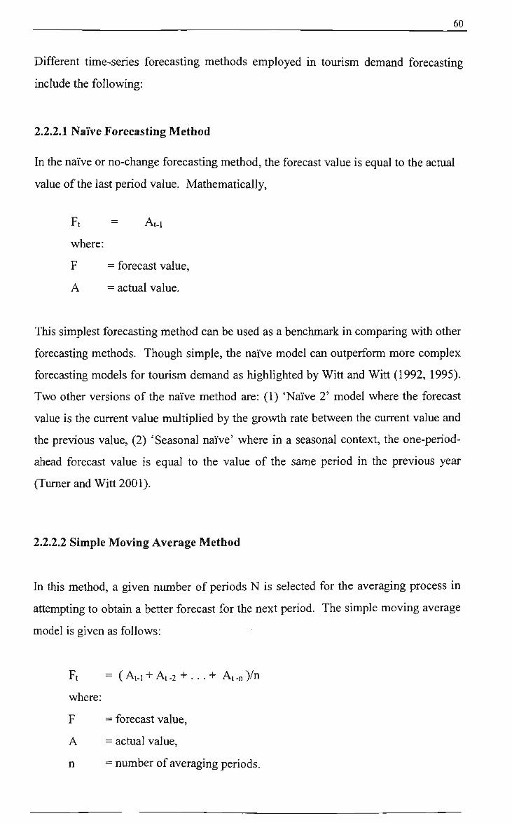
60_
Different time-series forecasting methods employed in tourism demand forecasting
include the following:
2.2.2.1 Naive Forecasting Method
In the naive or no-change forecasting method, the forecast value is equal to the actual
value of the last period value. Mathematically,
Ft = At.i
where:
F = forecast value,
A = actual value.
This simplest forecasting method can be used as a benchmark in comparing with other
forecasting methods. Though simple, the naive model can outperform more complex
forecasting models for tourism demand as highlighted by Witt and Witt (1992, 1995).
Two other versions of the naive method are: (1) 'Naive 2' model where the forecast
value is the current value multiplied by the growth rate between the current value and
the previous value, (2) 'Seasonal naive' where in a seasonal context, the one-period-
ahead forecast value is equal to the value of the same period in the previous year
(Tumer and Witt 2001).
2.2.2.2 Simple Moving Average Method
In this method, a given number of periods N is selected for the averaging process in
attempting to obtain a better forecast for the next period. The simple moving average
model is given as follows:
Ft = (At-i + At.2 + . . . + At.n)/n
where:
F = forecast value,
A = actual value,
n = number of averaging periods.

61
As a general principle, the longer the averaging period, the slower the response to
demand changes. Therefore, a longer period has the advantage of providing stability
in the forecast but the disadvantage of responding more slowly to real changes in the
demand level. Thus, the appropriate frade-off between stability and response of the
forecast must be made by selecting the average length n.
In the simple moving average method, all the past values used in the averagmg all
have the same influence on the forecast value. To make the moving average respond
more rapidly to changes in demand, relatively more weight (w) is placed on recent
demand than on earlier demand. This is knovm as the weighted moving average
approach and is computed as follows:
Ft =(wi At-i +W2At-2 +. . . + w„At-n)/n .
The advantage of the moving average method is its forecast simplicity. Disadvantages
of the weighted moving average method include: (a) the need to carry the entire
demand history for n periods for computation, and (b) the response of the weighted
moving average cannot be easily changed without changing each of the weights.
In summary, the moving-average method is one of the simplest methods of time-series
forecasting and assumes that the time series has only a level component and a random
component; that is no seasonal pattem, trend, or cycle components are present in the
time series data. In the results of a questionnaire survey by Martin and Witt (1988b),
it was indicated that the moving-average was the most popular technique for short-
term forecasting (less than one year ahead).
2.2.2.3 Decomposition Model
The classical decomposition approach decomposes a time series into four
components: trend, cycle, seasonal, and an irregular component. Therefore, a time
series can be represented as:

62
Xt = Tt x Ct X St X It or
Xt = Tt + Ct + St + It
where:
X represents the actual value in the time series,
T represents the trend component,
C represents the seasonal component,
S represents the seasonal component,
I represents the irregular component.
Thus the principle is to (1) identify these components and develop forecasts for each
using methods such as the moving average and regression, and (2) recombine the
individual forecasts to generate the final forecast.
The Census XI1 model developed for the US Bureau of the Census (Shiskin 1967) is
an example of the decomposition method. The X-11 program is used to deseasonalise
quarterly or monthly data thereby producing detailed analyses of seasonal factors, and
trend-cycle and irregular variations. The main disadvantage of X-11 is its inflexibility,
as the same procedure is essentially applied irrespective of the properties of the time
series.
2.2.2.4 Exponential Smoothing Methods
Intermediate extrapolative forecasting methods (Frechtling 1966, 2001) include: (1)
simple exponential smoothing, (2) double exponential smoothing, and (3)
autoregression. The single exponential smoothing method (Brovm 1963; Gardner
1985) equation is given as follows:
Ft = Ft-i + a(At-i - Ft-i)
where:
F = forecast value,
a = a smoothing constant between 0 and 1,
A - actual value.

63
From the equation, it can be seen that the higher the value of the smoothing constant,
the more weight it gives to the last value. A lower smoothing constant implies more
weight is given to all the values previous to the last value. Thus, the objective is to
obtain the smoothing constant value that will minimize the forecasting error measure.
The single exponential smoothing forecasting method is applicable to stationary time
series with no seasonality. Thus, it cannot always be applied directiy for tourism
arrival forecasting because of the seasonal effects that are present in a tourist arrival
data series. Differencing is used to derive stationary and to pre-process the seasonal
data series before using the single exponential forecasting to generate the forecast
values.
The double exponential smoothing method (Brovm 1963) was developed for ttended
time series, but its disadvantage is that is cannot deal with seasonality that is common
in tourism data series.
The triple exponential smoothing (Holt 1957; Winters 1960) method was developed
for a seasonal time series with ttend. The model is based on three equations
(Makridakis et al. 1998); one for level, one for ttend and one for seasonality.
Lt = a (At /S t . s )+ ( l -a ) (Lt . i+ Tt.i)
Tt = P(Lt-Lt . i )+ (l-P)Tt.,
St = y ( A t / L t ) + ( l - y ) S t . s
where:
L = level of the series,
a = level smoothing constant between 0 and 1,
A = actual value,
s = number of seasonal periods in a year,
T = trend of the series,
P = seasonal smoothing constant between 0 and 1,
S = seasonal component,
Y = seasonal smoothing constant between 0 and 1,

64
t = some time period,
h = number of time periods ahead to forecast.
Upon the determination of the values of the three smoothing constants, a, p and y the
forecast for m periods ahead is computed using the following equation:
Ft+h = (Lt+hTt) St-s + h
where:
h = number of time periods ahead to forecast.
The values of the three smoothing constants are calculated generally by the forecasting
system or statistical program internally and are chosen based on the minimum
absolute percentage error (MAPE) or mean square error (MSE) criterion (discussed
later in chapter 4).
In general, exponential smoothing methods are found to be most effective when the
components describing the time series are changing slowly over time (Bowerman and
O'Connell 1993).
Example Applications
Martin and Witt (1989) tested the accuracy of selected forecasting models (naive 1,
naive 2, exponential smoothing, trend curve analysis, Gompertz, autoregression, and
econometric) for outbound tourism from France, Germany, the United Kingdom, and
the United States to six of their main destinations. The results reveal that the simple
naive no-change extrapolation model generally generates the most accurate one-year-
ahead tourism demand forecasts with lower mean absolute percentage errors
(MAPEs).
Witt et al. (1992) applied the Holt-Winters, Naive 1 and Naive 2 models to generate
domestic forecasts of visitor arrivals in Las Vegas. The study shows that the Holt-
Winters exponential smoothing method generates forecasts with lower error
magnitudes (MAPE) than both the naive models for domestic tourism demand
65
forecasting in Las Vegas. This supported the suggestion that the Holt-Winters model
is particularly appropriate for data series where ttend and seasonality components are
present.
Athiyaman and Robertson (1992) use the following time-series forecasting techniques
to generate forecasts of intemational tourist arrivals from Thailand to Hong Kong: 1.
naive, 2. moving average, 3. single exponential smoothing, 4. linear moving average,
5. Brown's one-parameter linear exponential smoothing, 6. Holt's 2-parameter linear
exponential smoothing, and 7. Winter's 3-parameter exponential smoothing. Their
results confirm that simple techniques may be just as accurate and often more time-
and cost-effective than more complex ones.
Sheldon (1993) examined the accuracy of six different forecasting techniques (time
series and econometric causal models) to forecast annual tomism expenditures in the
United States by tourists from six origin countries (Canada, Japan, United Kingdom,
West Germany, France and Italy) for the years 1970 to 1986. The results show that
the accuracy of the forecasts, using MAPE, differs depending on the country being
forecast, but the no-change model and Brovm's double exponential smoothing are,
overall, the two most accurate methods for forecasting intemational tourism
expenditures.
Witt, Witt and Wilson (1994) examined the forecasting of quarterly outbound tourist
flows from tiie UK to four countries (Austtia, Greece, Italy and Spain). The
forecasting models (naive 1, naive 2, exponential smoothing, trend curve analysis,
Gompertz, autoregression, and ARIMA) were estimated over the period 1971 to 1987,
and used to forecast tourist flows for each quarter of 1988 and 1989. The forecasting
accuracy of the models were performed using MAPEs, and it was found that the
ARIMA forecasting model was the best performing model reflecting the suitability of
ARIMA for forecasting seasonal data as conducted in this study.
Witt and Witt (1995) reviewed the empirical research on forecasting tourism demand
and concluded that no single forecasting method performs consistently best across
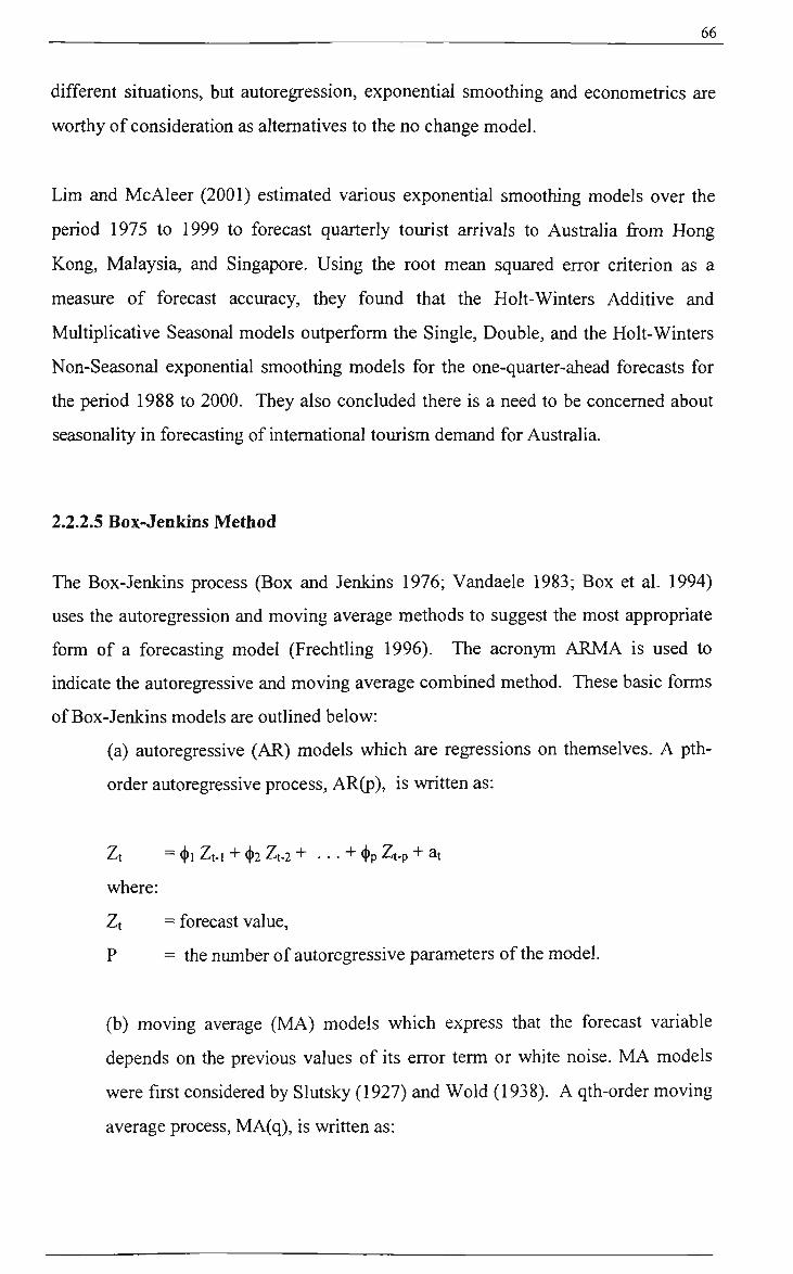
66
different situations, but autoregression, exponential smoothing and econometrics are
worthy of consideration as altematives to the no change model.
Lim and McAleer (2001) estimated various exponential smoothing models over the
period 1975 to 1999 to forecast quarterly tourist arrivals to Austtalia from Hong
Kong, Malaysia, and Singapore. Using the root mean squared error criterion as a
measure of forecast accuracy, they found that the Holt-Wmters Additive and
Multiplicative Seasonal models outperform the Single, Double, and the Holt-Winters
Non-Seasonal exponential smoothing models for the one-quarter-ahead forecasts for
the period 1988 to 2000. They also concluded there is a need to be concemed about
seasonality in forecasting of intemational tourism demand for Australia.
2.2.2.5 Box-Jenkins Method
The Box-Jenkins process (Box and Jenkins 1976; Vandaele 1983; Box et al. 1994)
uses the autoregression and moving average methods to suggest the most appropriate
form of a forecasting model (Frechtiing 1996). The acronym ARMA is used to
indicate the autoregressive and moving average combined method. These basic forms
of Box-Jenkins models are outlined below:
(a) autoregressive (AR) models which are regressions on themselves. A pth-
order autoregressive process, AR(p), is written as:
Zt = (f)} Zt-i + (j)2 Zt-2 + • • • + <f>p Zt-p + at
where:
Zt = forecast value,
P = the number of autoregressive parameters of the model.
(b) moving average (MA) models which express that the forecast variable
depends on the previous values of its error term or white noise. MA models
were first considered by Slutsky (1927) and Wold (1938). A qth-order moving
average process, MA(q), is written as:

67
Zt = at - 9i at-i - 02 at-2 - . . . - 9q at-q
where:
q = the number of moving average parameters.
(c) mixed autoregressive-moving average (ARMA) models, when the series is
partly autoregressive and partly moving average. An autoregressive moving
average process of orders p an q respectively, ARMA(p,q), is written as:
Zt = (|)i Zt-i + (|)2 Zt.2 + . . . + (|)p Zt-p + at - 61 at-i - 62 at-2 - . . . - % at-q .
A time series is known as stationary when its mean and variance do not change over
time. As ARMA models can only handle stationary time series, a non-stationary time
series would first be fransformed to become approximately stationary by applying
operations such as differencing. However, care is needed not to overdifference as this
can introduce unnecessary correlations into a model. If differencing is required to
achieve stationarity, then the series is eventually integrated before forecasting. In this
case, an I (for integrated) is added to ARMA model resulting in the
autoregressive/integrated/moving average or ARIMA model.
Mathematically, a nonseasonal stationary model resulting from d differencing, i.e.,
ARIMA (p,d,q) is written as:
Zt - Zt-i= (t)i (Zt-i - Zt-2) + ^2 (Zt-2 - Zt-3) + . . . + (|)p (Zt-p) +
at - 01 at-i - 02 at-2 - . . . - 0q at-q,
Yt = ()),Yt-i + (l)2Yt-2 + ... + (})pYt-p + at - Oiat-i -02at.2 -...-0qat-q
where:
Yt = Zt - Zt-i ,
Yt-(t)iYt-i - (t)2Yt-2 - ... - (l)pYt-p = at - 0iat.i -02 at-2 -...-0qat-q.
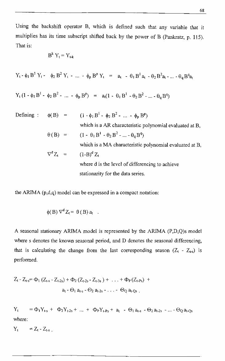
68_
Using the backshift operator B, which is defined such that any variable that it
multiplies has its time subscript shifted back by the power of B (Pankratz, p. 115).
That is:
B ' Yt = Yt-k
Y t - f B ^ Y t - (l)2B2Yt - ... - (t)pBPYt = at - 0iB^at -02B2at- . . . -OqB^
Yt (1 - (t)i B^ - (|)2 B ' - ... - (t)p BP) = at(l - 01B' - 02B" -... - OqB")
Defining : (|)(B) = ( l -( t ) ]B'- (j)2 B^ - ... - ^pB^)
which is a AR characteristic polynomial evaluated at B,
0(B) = ( 1 - OiB^ -02B^-.. .-0qB' ')
which is a MA characteristic polynomial evaluated at B,
V Z t = (l-B)''Zt
where d is the level of differencing to achieve
stationarity for the data series.
the ARIMA (p,d,q) model can be expressed in a compact notation:
(t)(B)V''Zt= 0(B) at .
A seasonal stationary ARIMA model is represented by the ARIMA (P,D,Q)s model
where s denotes the knovm seasonal period, and D denotes the seasonal differencing,
that is calculating the change from the last corresponding season (Zt - Zt-s) is
performed.
Zt - Zt-s= O i (Zt-s - Zt-2s) + O2 (Zt-2s - Zt-3s ) + . . . + O p (Zt-Ps) +
at - 0] at-s - 02 at.2s - . . . - 0 Q at-Qs ,
Yt =0,Yt-s+ 02Yt-2s+ ... + OpYt-Ps+ at - 0iat-s -02at-2s -...-©Qat-Qs
where:
Yt = Zt - Zt-s,
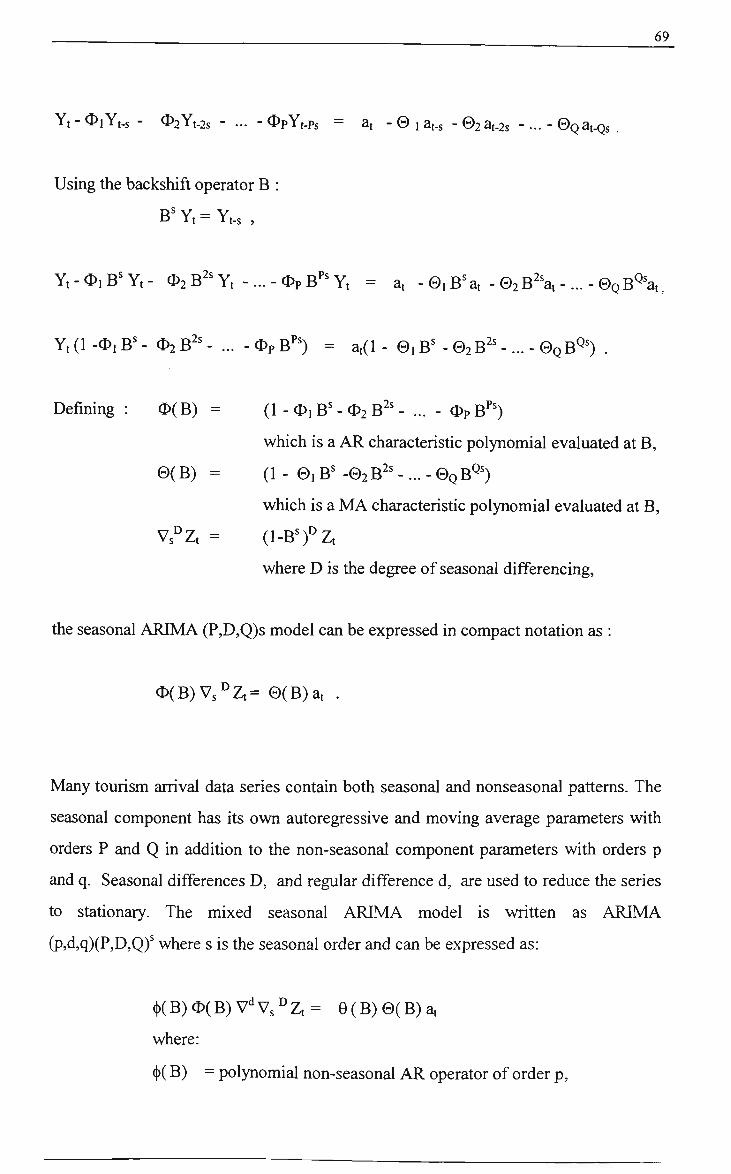
69
Yt - OiYt-s - 02Yt-2s - ... - OpYt-Ps = at - 0 1 at-s - 02at.2s -... - ©gat-Qs.
Using the backshift operator B :
B^ Yt = Yt-s ,
Yt-OiB^Yt- O2 B'^ Yt -... - Op B''^ Yt = a, -OiB^at - 0 2 B ' % - . . . - © Q B ^ ^ ,
Yt (1 -O, B^ - O2 B^' - ... - Op B''') = at(l - ©i B' - ©2 B^' - . . . - ©QB^^) .
Defining : 0 (B) = (1 - O j B ' - O s B ^ ' - ... - OpB''')
which is a AR characteristic polynomial evaluated at B,
©(B) = (1 - ©1B^ -©2 B^' -... - 0Q B^')
which is a MA characteristic polynomial evaluated at B,
Vs' Zt = (l-B^)°Zt
where D is the degree of seasonal differencing,
the seasonal ARIMA (P,D,Q)s model can be expressed in compact notation as :
0 (B)Vs°Zt= ©(B)at .
Many tourism arrival data series contain both seasonal and nonseasonal pattems. The
seasonal component has its ovm autoregressive and moving average parameters with
orders P and Q in addition to the non-seasonal component parameters with orders p
and q. Seasonal differences D, and regular difference d, are used to reduce the series
to stationary. The mixed seasonal ARIMA model is written as ARIMA
(p,d,q)(P,D,Q)^ where s is the seasonal order and can be expressed as:
7dv7 D . ())(B)0(B)V' 'V3"Zt- 0(B) ©(B) at
where:
(j)( B) = polynomial non-seasonal AR operator of order p.

70
0( B) = polynomial non-seasonal MA operator of order q,
0 ( B) = polynomial seasonal AR operator of order P,
©( B) = polynomial seasonal MA operator of order Q, and
V Vs° = differencmg operators.
The Box-Jenkins modelling methodology, shovm in Figure 2.1, has the following five
stages (Frechtiing 1996,2001):
(1) Preparation
- the data series is first examined for stationarity and seasonality. Seasonality
in the series can be determined by using the autocorrelated coefficients. The
data is then pre-processed to achieve mean and variance stationarity.
(2) Model identification
- the data series estimated autocorrelation and partial autocorrelation
coefficients are displayed graphically using the estimated autocorrelation
function (acf) and partial autocorrelation function (pacf). An estimated
autocorrelation function (acf) shows the correlation between ordered pairs
from a time series, separated by various time spans; and an estimated partial
autocorrelation fimction (pacf) which shows the correlation between ordered
pairs from a time series, separated by various time spans, with the effects of
intervening observations accounted for.
To identify a tentative model with the values of p,d and q, a visual
examination and comparison is then made between the theoretical and
estimated acf s and pacf s, with the objective of finding a model that is
parsimonious and statistically adequate. A time-dependent process has a
theoretical acf and pacf and the estimated acf s and pacf s are found by
applying the autocorrelation coefficient statistic and Yule-Walker equations
(Pankratz, 1983). Estimated acf s and pacf s never match theoretical acf s
and pacf s exactly due to sampling error. The decision matrix for identifying
the appropriate form of the ARMA model using the acf and pacf is shovm in
Table 2.1

70
0( B) = polynomial non-seasonal MA operator of order q,
0 (B) = polynomial seasonal AR operator of order P,
©( B) = polynomial seasonal MA operator of order Q, and
V Vs = differencing operators.
The Box-Jenkins modelling methodology, shown in Figure 2.1, has the following five
stages (Frechtiing 1996,2001):
(1) Preparation
- the data series is first examined for stationarity and seasonality. Seasonality
in the series can be determined by using the autocorrelated coefficients. The
data is then pre-processed to achieve mean and variance stationarity.
(2) Model identification
- the data series estimated autocorrelation and partial autocorrelation
coefficients are displayed graphically using the estimated autocorrelation
function (acf) and partial autocorrelation function (pacf). An estimated
autocorrelation function (acf) shows the correlation between ordered pairs
from a time series, separated by various time spans; and an estimated partial
autocorrelation function (pacf) which shows the correlation between ordered
pairs from a time series, separated by various time spans, with the effects of
intervening observations accounted for.
To identify a tentative model with the values of p,d and q, a visual
examination and comparison is then made between the theoretical and
estimated acf s and pacf s, with the objective of finding a model that is
parsimonious and statistically adequate. A time-dependent process has a
theoretical acf and pacf and the estimated acf s and pacf s are found by
applying the autocorrelation coefficient statistic and Yule-Walker equations
(Pankratz, 1983). Estimated acf s and pacf s never match theoretical acf s
and pacf s exactly due to sampling error. The decision matrix for identifying
the appropriate form of the ARMA model using the acf and pacf is shovm in
Table 2.1

71
Table 2.1
ARMA models decision matrix
Model (order) AR(p) MA(q) ARMA (1,1)
Autocorrelations (acf) Tail off toward zero Cuts off to zero after lag q Tails off towards zero
Partial Autocorrelations (pacf) Cuts off to zero after lag p Tails off toward zero Tails off towards zero
(3) Model estimation
- the tentative ARMA model parameters ((j) and 0) are then estimated based on
the iterative maximum likelihood (ML) process (Norden, 1972). The final
values of (j) and 0 are based on their combination to minimise the sum of the
squared errors.
(4) Diagnostic checking
- Once the tentative model has been estimated, a residual analysis diagnostic
check can be made of the model. The fitted residuals should be white noise ;
that is it should have a mean of zero, a constant covariance, and be
uncorrelated with each other over time. These assumptions can be examined
by visual examination of the residuals plot in tiie diagnostic checking process.
Also, tiie Box-Pierce Q statistic and the modified Box-Pierce (or Ljung-Box)
Q* statistic can be applied to check that there are no significant
autocorrelations in the fitted model's error terms. If the t-tests on the
estimated parameters show that tiiey are significantiy different from zero, and
tiie fitted residuals are white noise, then the model is deemed to be adequate.
Should the model fail the diagnostic checks, the cycle is repeated until a
satisfactory model is foimd. When final model selection is needed from
various competing possible models, the Akaike information criterion (AIC)
(Akaike, 1973, 1974, 1979) and Schwartz Baynesian criterion (SBC) can be
used to aid in selecting tiie most appropriate model. Ideally, the AIC and SBC
should be as small as possible.

72
(5) Forecasting
- The fitted model is used to forecast future values of time series. Once the
forecasts are obtained, fransformation of the values back to into the term of the
original series is taken, if necessary.
Characteristics of a good ARMA or ARIMA model (Pankratz, 1983) are that (a) it is
parsimonious, i.e. the model uses a small number of parameters or coefficients to
explain the available data, (b) it is stationary, (c) it is mvertible, (d) it has high quality
estimated coefficients, (e) it has uncorrelated residuals, (f) it fits the available data
satisfactorily, that is, it has acceptable root-mean-squared error (RMSE) and mean
absolute percent error (MAPE) values, and (g) it produces accurate forecasts.
Advantages of ARIMA models are: (a) ARIMA models are based on a solid
foundation of classical probability theory and mathematical statistics (Pankratz
1983), (b) Versatility of the ARIMA models for various types of time series. For
example, exponential smoothing methods can handle only time series with
deterministic frend in which the average level of the series grows or declines
according to some specific function in time. However, many time series display
stochastic frends, i.e. ttends with variable rates of growth. Both deterministic and/or
stochastic ttend can be modelled using ARIMA models (Famum and Stanton 1989),
and (c) Unified, theoretically sound approach to forecasting. That is, the Box-Jenkins
methodology provides a systematic approach to model selection, utilising all the
information available in the sample acf and pacf
Disadvantages of the Box-Jenkins method are: (a) the method is fairly complicated
and considerable expertise is required in specifying a suitable model using the sample
and partial autocorrelation functions, particularly in small samples, (b) difficulties of
interpretation, and (c) attempts to select ARIMA models by an automatic procedure,
such as the AIC can lead to worse results (Harvey and Todd 1983). Consequently,
statistical packages which purport to offer automatic ARIMA selection are severely
limited, (d) the method requires about at least 50 observations as the minimum
amount of data in the time series (Box and Jenkins 1976), and (e) it does not
necessarily guarantee better forecasts than simpler forecasting techniques.
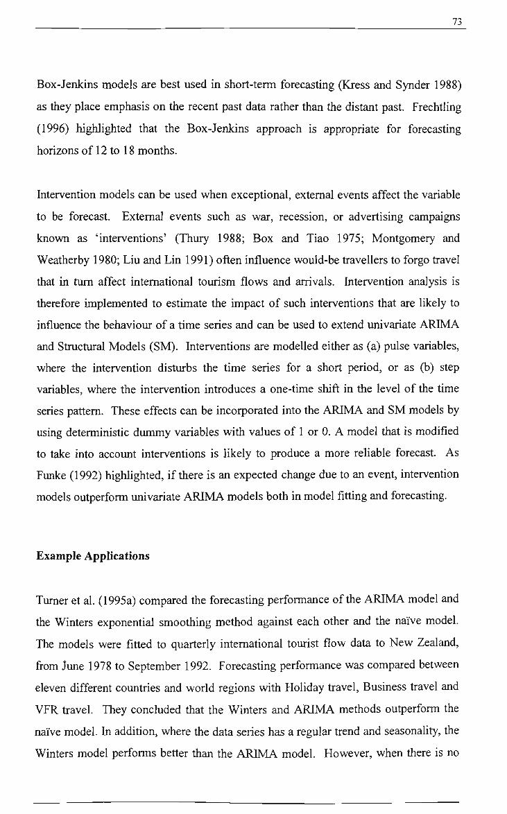
73
Box-Jenkins models are best used in short-term forecasting (Kress and Synder 1988)
as they place emphasis on the recent past data rather than the distant past. Frechtiing
(1996) highlighted that the Box-Jenkins approach is appropriate for forecasting
horizons of 12 to 18 months.
Intervention models can be used when exceptional, extemal events affect the variable
to be forecast. Extemal events such as war, recession, or advertising campaigns
knovm as 'interventions' (Thury 1988; Box and Tiao 1975; Montgomery and
Weatherby 1980; Liu and Lin 1991) often influence would-be ttavellers to forgo ttavel
that in tiim affect intemational tourism flows and arrivals. Intervention analysis is
therefore implemented to estimate the impact of such interventions that are likely to
influence the behaviour of a time series and can be used to extend univariate ARIMA
and Stmctural Models (SM). Interventions are modelled either as (a) pulse variables,
where the intervention disturbs the time series for a short period, or as (b) step
variables, where the intervention inttoduces a one-time shift in the level of the time
series pattem. These effects can be incorporated into the ARIMA and SM models by
using deterministic dummy variables with values of 1 or 0. A model that is modified
to take into account interventions is likely to produce a more reliable forecast. As
Funke (1992) highlighted, if there is an expected change due to an event, intervention
models outperform univariate ARIMA models both in model fitting and forecasting.
Example Applications
Tumer et al. (1995a) compared the forecasting performance of the ARIMA model and
the Winters exponential smoothing method against each other and the naive model.
The models were fitted to quarterly intemational tourist flow data to New Zealand,
from June 1978 to September 1992. Forecasting performance was compared between
eleven different countries and world regions with Holiday travel, Business fravel and
VFR ttavel. They concluded that the Winters and ARIMA methods outperform tiie
naive model. Lti addition, where the data series has a regular ttend and seasonality, the
Winters model performs better than the ARIMA model. However, when there is no
74
highly significant ttend and seasonality, the ARIMA forecasting model performs
better.
Dharmaratne (1995) estimated ARIMA models for forecasting long-stay annual
visitors arrivals in Barbados with data from 1956-87 and from 1956-91, to facilitate
testing of the long-term (5-year) and short-term (2-year) forecasting ability of the
models. The accuracy of the ex post forecasts were compared using MAPE. It was
found that the ARIMA (2, 1,1) model provides excellent forecasts for both the long-
term and short-term forecasts of tourist arrivals in Barbados. Therefore, he concluded
that customized forecasting model building may be highly rewarding as the value of a
forecasting model depends on the accuracy of out-of-sample forecasts that can be
generated from the model.
Chu (1998a) performed the forecasting of annual total tourist arrivals into Singapore
using seasonal and non-seasonal ARIMA models. Data from July 1977 to December
1988 were used to forecast the tourist arrivals for the following 19 months (January
1989 to July 1990). The empirical results showed that tiie ARIMA (3, 1, 0) (0, 1, 0)
forecasting model tumed out to be relatively accurate among several other forecasting
methods including a nonlinear sine wave time-series regression model. Chu
concluded that although the proposed ARIMA model needed a reasonable amount of
data to implement, the gain in forecasting accuracy over the naive model was worth
the effort.
Chu (1998b) examined forecasting models using monthly intemational tourist arrivals
data in 10 countries (Taiwan, Japan, Hong Kong, South Korea, Singapore, the
Philippines, Indonesia, Thailand, New Zealand, and Australia). The models are fitted
to the arrivals in these countries between January 1975 and December 1994. Tourist
arrival forecasts were made from January 1995 to June 1996. The forecasting
accuracy was compared based on the smallest MAPE value, and it was found to differ
between countries. Overall, the seasonal-non-seasonal ARIMA models were found to
be the most accurate forecasting method in nine out of ten countties. Holt-Winters

75
were found to perform marginally better than the ARIMA model for New Zealand
arrivals.
Chan, Hui and Yuen (1999) highlighted that most forecasting models for tourist
arrivals were constmcted under the assumption of only minor changes in the
environment; and the performance of forecasting models in situations of sudden,
drastic environmental change(s) has not been given much attention. Using the Gulf
War as an example of sudden environmental change, the study explored the relative
performance of different forecasting models which include: (1) ARIMA (p,d,q) model,
(2) exponential smoothing, (3) naive I, (4) naive II, and (5) frend curve analysis. Six
sets of data were used that included total tourist arrivals in Singapore as well as
arrivals from the United States, Japan, United Kingdom, Germany, and Austtalia. For
each of the five forecasting techniques, the mean absolute percentage error (MAPE)
was the criterion used to measure the accuracy of the forecastmg model. The findings
showed that in terms of forecasting accuracy, the naive II model performs better than
other techniques in this study.
Lim and McAleer (2002) estimated various Autoregressive Moving Average (ARMA)
models over the period 1975(1) to 1996(12) for monthly tourist arrivals to Australia
from Hong Kong, Malaysia and Singapore. The Akaike Information Criterion and the
Schwartz Baynesian Criterion was used to select the best fitting ARMA model to
obtain post-sample forecasts. They found that the fitted seasonal ARIMA models
outperform the non-seasonal ARMA models. In particularly, the fitted ARIMA
(0,1,1) model for the seasonally adjusted data series performed better than the non-
seasonally adjusted ARMA (12,2) model for Singapore monthly tourist arrivals to
Austtalia.
Gob and Law (2002) applied ARIMA models with interventions in forecasting
tourism demand using ten arrival series for Hong Kong. The forecasts obtained using
these intervention models captured stochastic nonstationary seasonality and
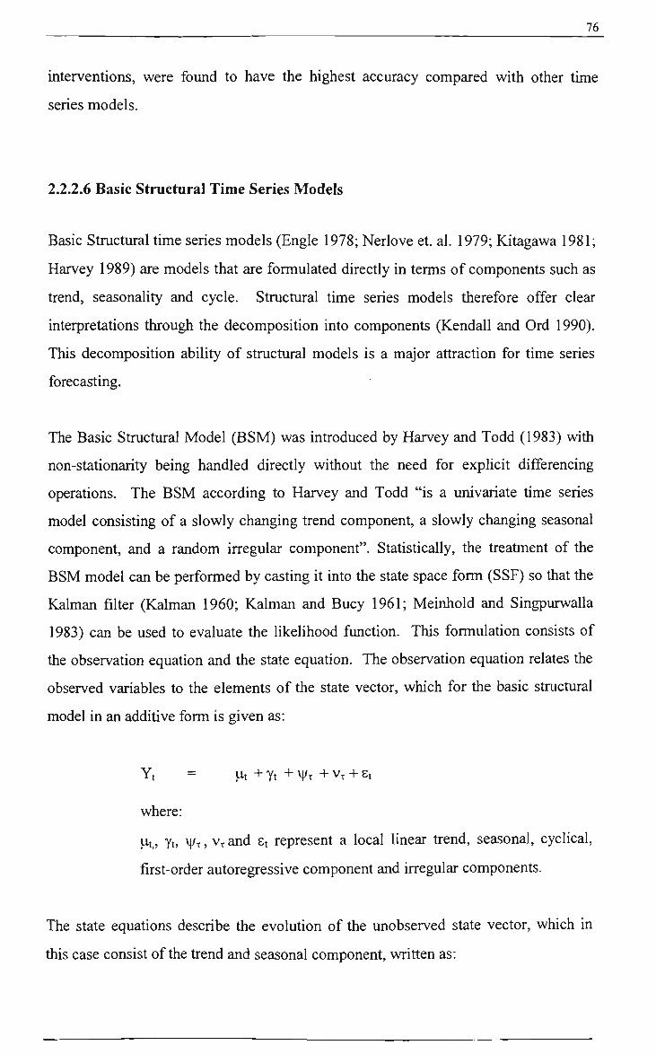
76
interventions, were found to have the highest accuracy compared with other time
series models.
2.2.2.6 Basic Structural Time Series Models
Basic Structural time series models (Engle 1978; Nerlove et. al. 1979; Kitagawa 1981;
Harvey 1989) are models that are formulated directly in terms of components such as
ttend, seasonality and cycle. Stmctural time series models therefore offer clear
interpretations through the decomposition into components (Kendall and Ord 1990).
This decomposition ability of stmctural models is a major attraction for time series
forecasting.
The Basic Stmctural Model (BSM) was introduced by Harvey and Todd (1983) with
non-stationarity being handled directly without the need for explicit differencing
operations. The BSM according to Harvey and Todd "is a univariate time series
model consisting of a slowly changing ttend component, a slowly changing seasonal
component, and a random irregular component". Statistically, the tteatment of the
BSM model can be performed by casting it into the state space form (SSF) so that the
Kalman filter (Kalman 1960; Kalman and Bucy 1961; Meinhold and Singpurwalla
1983) can be used to evaluate the likelihood function. This formulation consists of
the observation equation and the state equation. The observation equation relates the
observed variables to the elements of the state vector, which for the basic stmctural
model in an additive form is given as:
Yt = |it + Yt + H/x + VT + St
where:
l t,, Yt, VT , Vx and 8t represent a local linear trend, seasonal, cyclical,
first-order autoregressive component and irregular components.
The state equations describe the evolution of the unobserved state vector, which in
this case consist of the trend and seasonal component, written as:
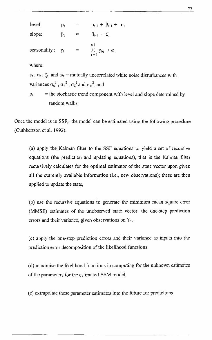
77
level: ^t = Ht-i + Pt-i + lit
slope: pt = Pt-i + Ct
s-l
seasonality: yt = S Yt-j + ©t j = i
where:
Et, rit, C,t and cot = mutually uncorrelated white noise disturbances with
variances Gg , a ^ , CQ and ao^, and
fit = the stochastic trend component with level and slope determined by
random walks.
Once the model is in SSF, the model can be estimated usmg the follovving procedure
(Cutiibertson et al. 1992):
(a) apply the Kalman filter to the SSF equations to yield a set of recursive
equations (the prediction and updating equations), that is the Kalman filter
recursively calculates for the optimal estimator of the state vector upon given
all the currently available information (i.e., new observations); these are then
applied to update the state,
(b) use the recursive equations to generate the minimum mean square error
(MMSE) estimates of the unobserved state vector, the one-step prediction
errors and their variance, given observations on Yt,
(c) apply the one-step prediction errors and their variance as inputs into the
prediction error decomposition of the likelihood functions,
(d) maximise the likelihood fimctions in computing for the unknovm estimates
of the parameters for the estimated BSM model,
(e) exttapolate these parameter estimates into the future for predictions.
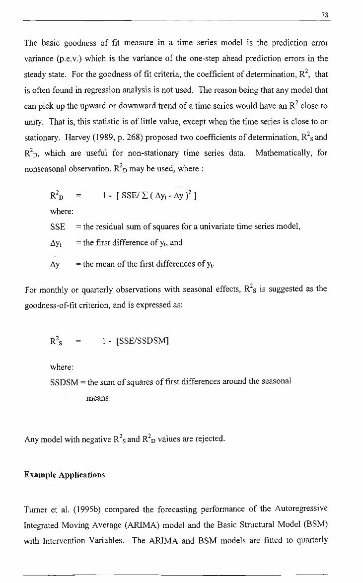
78
The basic goodness of fit measure in a time series model is the prediction error
variance (p.e.v.) which is the variance of the one-step ahead prediction errors m the
steady state. For the goodness of fit criteria, the coefficient of determination, R , that
is often found m regression analysis is not used. The reason being that any model that
can pick up the upward or downward ttend of a time series would have an R close to
unity. That is, this statistic is of little value, except when the time series is close to or
stationary. Harvey (1989, p. 268) proposed two coefficients of determination, R s and
R D, which are useful for non-stationary time series data. Mathematically, for
nonseasonal observation, R D may be used, where :
R'D = 1- [SSE/S(Ayt-Ay) ']
where:
SSE = the residual sum of squares for a univariate time series model,
Ayt = the first difference of yt, and
Ay = the mean of the first differences of yt.
For monthly or quarterly observations with seasonal effects, R s is suggested as the
goodness-of-fit criterion, and is expressed as:
R s = 1 - [SSE/SSDSM]
where:
SSDSM = the sum of squares of first differences around the seasonal
means.
Any model with negative R s and R^D values are rejected.
Example Applications
Tumer et al. (1995b) compared the forecasting performance of the Autoregressive
hitegrated Moving Average (ARIMA) model and the Basic Stmctural Model (BSM)
with Intervention Variables. The ARIMA and BSM models are fitted to quarteriy

79
tourist flows into Austtalia and New Zealand, from the USA, Japan, and the UK. The
model estimation period was from 1978 (Jime) to 1993 (September), and eight
quarters (December 1991 to September 1993) were used as the post-sample period to
assess the forecasting performance of the models. It was found that the BSM model
showed a consistently high performance against the ARIMA model. In addition the
forecast errors were reduced when intervention variables (such as special events) were
added to the models. They highlighted that tourism practitioners will find it
worthwhile to look at BSM modelling in the fiiture.
Tumer and Witt (2001) analysed forecasting of inbound tourism to New Zealand from
Australia, Japan, the UK and the USA disaggregated by purpose of visit using both the
Basic Stmctural Model (BSM) and the muhivariate stmctural time series model. The
stmctural time series models were estimated over the 2" " quarter 1978 to 4* quarter
1995, leaving a post-estimation period of eleven quarters from 1** quarter 1996 to 3'
quarter 1998 for forecasting performance assessment. The respective forecasting
accuracy of the models is compared using MAPEs. The findings are that the stmctural
time series model is reasonably accurate and outperformed the seasonal naive model;
and the multivariate stmctural time series model does not generate more accurate
forecasts than the BSM model. They concluded that the stmctural time series model
can reduce overall forecast error by 2% to 3% against tiie seasonal naive model and
tills was important, because this has not been found to be case for causal based
models.
Greenidge (2001) utilized Sttncttiral Time Series Modeling to explain and forecast
tourist arrivals to Barbados from its major generating markets and found these models
offered valuable insights into the stylized facts of tourism behavior and provided
reliable out-of-sample forecasts.

80
2.2.2.7 Neural Networks
The application of Artificial Neural Networks (ANNs) in forecasting as an altemative
to fraditional statistical methods have been well reviewed by Hill et al. (1994), Warner
and Misra (1996), and Zhang et al. (1998). Denton (1995) highlighted that tiie Neural
Network offers an altemative to multiple regression for performing causal forecasts,
hi particular, under less than ideal conditions. Neural Networks do a better job. That
is, the Neural Network forecasting method eliminates the ambiguities present in
selecting the appropriate independent variables needed in defmmg a multiple
regression model. This is important as performing a statistical regression v^th a mis-
specified model can result in biased and inconsistent parameter estimates. In Hill et al.
(1996) study, time series forecasts produced by Neural Networks are compared with
forecasts from 6 statistical time series methods generated in a major forecasting
competition (Makridakis et al. 1982). The ttaditional method forecasts are estimated
by experts in the particular techniques. It was found that across monthly and quarterly
time series, the Neural Networks did significantly better than ttaditional methods.
Refenes et al. (1994) also highlight that traditional statistical techniques for
forecasting have reached their limitations in applications with non-linearities in the
data set, such as stock indices.
ANN Overview
The artificial Neural Network (ANN) (Simpson 1990; Carling 1992; Haykin 1994;
Rojas 1996; Taylor 1998) consists of a number of processing elements, normally
arranged in layers. Each processing element is linked to elements in the previous
layer by connections that have an adaptable strength or weight. The adaptation of
these weights is performed by a leaming algorithm. It is this adaptation of these
weights that gives the Neural Network its capability to leam by example thereby
capturing the functional relationships within the data (White 1989; Koster et al. 1990;
Ripley 1993; Cheng and Titterington 1994). ANN has been mathematically shovm to
be a universal approximator of functions and their derivatives (Cybenko 1989; Homik
et al. 1989; White et al. 1992). Unlike ttaditional statistical metiiods, ANN do not

81
require assumptions about the form or distribution of the data to analyze it, and are
more tolerant of imperfect data, and therefore estimate norUinear functions well
(Lapedes and Farber 1987; Gorr 1994; Hill and Remus 1992, 1994; Zhang 1998) and
discontinuous functions (Wasserman 1989; Marquez et al. 1991). After the network
has been trained and validated, the model may be applied to suitable neural
computations such as prediction, classification, time-series forecasting or data
segmentation.
ANN models have two leaming methods, supervised and imsupervised. Time-series
forecasting neural computation involves the use of a class of neural models knovm as
supervised Neural Networks. These networks require both inputs and targets. The
leaming algorithm modifies the network weights so that the model leams the mapping
from input to target. The different supervised artificial Neural Networks known for
time-series forecasting are Multi-Layer Perceptton, Radial Basis Function, and
Bayesian Neural Network. An overview of the architecture, activation function, and
training algorithm for these Neural Networks is discussed below.
The Multi-Layer Perceptron
The MLP is perhaps the most popular network architecture in use (Rumelhart and
McClelland 1986; Haykin 1994; Bishop 1995). The MLP is a Neural Network that is
based on the original Simple Perceptton model but with additional hidden layers of
neurons between the input and output layers. This hidden layer vastly increases tiie
leaming power of the MLP. The inputs to each processing element, or nodes, are
usually fiilly connected to the outputs of the previous layer. Typically, the mcoming
signals to a node are combined by summing their weighted values. This is represented
mathematically as:
n netj = X xiwij
i= l
where:
netj = the resultant combined input to node j .
82
xi = the output from node i, and,
n = the number of impinging connections.
The leaming algorithm modifies the weights associated with each processing element
such that the system minimizes the error between the target output and the network's
actual output. The number of nodes is directiy related to the complexity of the system
being modelled. The most widely use MLP Neural Network ttaining or leaming
algorithm is back propagation (Rumelhart et al. 1986; Patterson 1996; Haykin 1994;
Fauset 1994). The backpropagation algorithm was first developed by Werbos (1974)
and has been actively adopted for use vsith Neural Networks. In the backpropagation
training algorithm, there is a forward pass through the Neural Network to determine
the network's current outputs, followed by a backward pass to determine, based on the
difference between these outputs and the correct ones, how the weights should be
changed. Training begins with arbitrary values for the weights. In each iteration,
called epoch, the network adjusts the weights in the direction that reduces the error.
As the iterative process continues, the weights gradually converge to an optimal set of
values.
The method of determining the amount of change is known as the leaming law. Two
commonly used learning laws are Steepest Descent and Conjugate Gradient. For
Steepest Descent, at the completion of a pass, all the nodes change their weights based
on the accumulative derivatives of the error with respect to each weight. These
weight changes move the weight in the direction in which the error declines most
quickly. The Conjugate Gradient method (Bishop 1995) also called 'backpropagation
with momentum' is one of the second-order methods of deciding weight change.
Second-order methods involve calculating an approximation of the second derivative
of the error with respect to a weight and using this quantity, in conjunction with the
first derivative, to decide the amount of the weight change.
There are also heuristic modifications of back propagation which work well for some
problem domains, such as quick propagation (Fahlman 1989) and Delta-Bar-Delta
(Jacobs 1988). In most cases, they are not significantly better than back propagation,
and sometimes they are worse (relative performance is application-dependent). They

. 83_
also require more control parameters than any of the other algorithms, which makes
them more difficuh to use.
During the forward pass through the MLP, each node output is computed from its
inputs based on several possible 'activation' or 'transfer' functions such as sigmoid,
linear, and hyperbolic tangent (tanh). Mathematically,
Sigmoid: f(net) = 1/1+ exp(-net) .
Tanh: f(net) = [exp(net) - exp(-net)]/ [exp(net) + exp(-net)]
Where:
f(net) = the node output using the ttansfer fimction,
net = the resultant combined inputs to the node,
exp = the constant with value of about 2.71828.
MLP models generally use a sigmoid activation function, with continuous activations,
mostly chosen from [0,1] or [-1,1].
Important issues in Multilayer Perceptrons (MLP) design include the specification of
the number of hidden nodes and the leaming algorithm for the network (Haykin 1994;
Bishop 1995). If there are too many hidden nodes for the problem, the network can
become too specific or over-trained. Fimahashi (1989) has shown mathematically that
only one hidden layer is needed to model a network to fit and fimction optimally; and
Hecht-Nelson (1989) show that there need be no more than 2n+l hidden layer nodes,
for n input nodes. Therefore, developing an MLP requires a certain degree of
experimentation. The error of a particular configuration of the MLP network can be
determined by miming all the training cases through the network, and comparing the
actual output generated with the desired or target outputs. The differences are
combined together by an error function to give the network error. The most common
error fimctions are the sum squared error (used for regression problems), where the
individual errors of output units on each case are squared and summed together, and
the cross enfropy fimctions (used for maximum likelihood classification).
84
The Radial Basis Function
Another model used in time-series forecasting is the Radial Basis Fimction network,
or RBF (Broomhead and Lowe 1989; Moody and Darkin 1989; Leonard et al. 1992;
Haykin 1994). It is a supervised, feed-forward Neural Network with one hidden layer
of artificial neurons. RBF is also used for supervised leaming, but uses different
activation fimctions than multilayer perceptions. The advantages of RBF models are
that they can model any nonlinear function using a single hidden layer, which removes
some design-decisions about numbers of layers, and the fraining is much more rapid
than with the MLP since they train in one stage rather than using an iterative process.
hi the RBF network the outputs that form the hidden layer are treated as a measure of
how far away the data are from a centte. The ttansfer functions of the nodes are
nonlinear. The ttansfer function used is known as the Radial Basis Functions, which
is a linear combination of nonlinear basis fimctions.
The most common ttansfer functions used in Radial Basis Functions are radial spline,
Gaussian, Quadratic, and Inverse Quadratic.
The Baynesian Network
Lastly but not least, tiie Bayesian Network (BAYN) is a modified MLP network for
time-series forecasting designed to avoid over-fitting. The Bayesian network applies
Bayes Theorem to the MLP. The Bayesian theory adds an extra term to tiie error
measure that reduces the impact of noise on the network.
Performance measures
The metiiod for validating the performance of a Neural Network in time-series
forecasting is based on the measurements of the residuals; that is the differences

85
between the output of the Neural Network model and the actual values in the time
series. These different measures of accuracy in forecasting (Makridakis et al. 1983,
1998) are: MSE, RMSE, and MAPE. They will be discussed fiirtiier in next chapter.
Li addition, Adya and Collopy (1998) highlighted how effectively a Neural Network
technique was compared with other forecasting methods and how well the Neural
Network technique was implemented, is a key area to consider before concluding on
the effectiveness of Neural Networks for forecasting and prediction.
ANN Modelling Issues
Zhang et al. (1998) has reviewed the main ANN modelling issues which include: (1)
the network architecture, which mclude determining the number of input nodes, the
number of hidden layers and hidden nodes, and the number of output nodes; (2) the
activation function, and (3) the ttaining algorithm, (4) the ttaining sample and test
sample, and (5) performance measures. Similarly, Walczak (2001) highlighted several
design factors that can significantly impact on the accuracy of Neural Network
forecasts. These factors include selection of input variables, architecture of the
network, and quantity of ttaining data.
Another issue with the use of Neural Networks comes essentially from their power as
a universal approximator. In general, a complex (in terms of numbers of hidden
layers) network will be able to fit any data set perfectly. When this happens, over-
fitting occurs, that is the Neural Network will offer good explanatory power within
their ttaining sample but they may breakdovm completely out of the sample. Thus, it
is an art to achieve a sufficiently good fit without over-fitting.
Also the question of whether the data should be deseasonalized first for time series
forecasting using Neural Networks was raised by Nelson et al. (1999). Their findings
using forecasts for 68 monthly time series from the M-competition (Makridakis et al.
1982) indicated that when there was seasonality in the time series, forecasts from
Neural Networks estimated on deseasonalized data were significantiy more accurate
than the forecasts produced by Neural Networks that were estimated using data which
were not deseasonalized. They highlighted that the mixed results from past studies of

86
ANN forecasting accuracy may be due to inconsistent handling of seasonality. It
caimot be assumed that the Neural Network model can build seasonal effects into its
leaming process.
In summary, there is no formal systematic ANN model building approach (Qi and
Zhang 2001). For instance, there is no standard formula for calculating the number of
layer and nodes needed in the hidden layer (Lippman 1987; Gorr et al. 1994; Turban
1995; Jeng and Fesenmaier 1996). In particular, the problem of network ''tuning"
remains: parameters of the backpropagation algorithm as well as the Neural Network
design need to be adjusted for optimal performance. Therefore, there is no one single
ANN configuration that is suitable for all applications; and a process of trial and error
is needed to find the right parameters for an ANN forecasting model.
Example Applications
Neural Networks has been used in many business areas (Widrow et al. 1994; Ansuj et
al. 1996; Wong et al. 2000; Smith and Gupta 2002). One major application of Neural
Networks is in financial forecasting (Refenes 1995; Qi 1996; Cheng et al. 1997;
Fadlalla and Lin 2001). Some of these studies are highlighted below.
Chiang et al. (1996) applied a backpropagation artificial Neural Network to forecast
tiie end-of-year net asset value (NAV) of mutual fimds. The results of the forecasting
are compared to those of traditional econometric techniques (linear and nonlinear
regression analysis), and it was shovm that Neural Networks significantiy outperform
regression models in situations with limited data availability.
Zhang and Hu (1998) in their application of Neural Network forecasting of the British
pound/US dollar exchange rate highlighted that researchers often overiook the effect
of Neural Network parameters on the performance of Neural Network forecasting.
They found that Neural Networks outperform linear models, particularly when the
forecast horizon is short. In addition, the number of input nodes has a greater impact
on performance than the number of hidden nodes, while a larger number of
observations do reduce forecast errors.
87
Aiken (1999) presented the findings of Consumer Price Index (CPI) forecasts from an
artificial Neural Network using leading economic mdicator data in the USA. The
resuhs show that the Neural Network predicts the level of the CPI with a high degree
of accuracy.
Yao and Tan (2000) in their forecasting of the option prices of Nikkei 225 index
futures using backpropagation Neural Networks found that different resuhs in terms of
accuracy are achieved by grouping the data differentiy. The results suggested tiiat for
volatile markets a Neural Network option pricing model outperforms the ttaditional
Black-Scholes model. However, the Black-Scholes model is still good for pricing at-
the-money options.
Moshiri and Cameron's (2000) study compared the performance of Back Propagation
Artificial Neural Network (BPN) models with the traditional approaches to forecasting
the inflation rate. The ttaditional models included a stmctural reduced-form model, an
ARIMA model, a vector autoregressive model, and a Bayesian vector autoregression
model. Each model is compared with a hybrid BPN model that uses the same set of
variables. Dynamic forecasts are compared for three different horizons: one, three and
twelve months ahead. The results show the hybrid BPN models are able to forecast as
well as all the ttaditional methods, and to outperform them in some cases.
Tkacz (2001) in his Neural Network forecasting of Canadian GDP growth found that
Neural Networks yield statistically lower forecast errors for the year-over-year growth
rate of real GDP relative to linear and univariate models. However, such forecast
improvements are less notable when forecasting quarterly real GDP growth.
More recentiy, Neural Networks have been applied to tourism demand forecasting.
Pattie and Snyder (1996) utilised a Neural Network to forecast over-night backcountry
stays in US national parks. Comparison of classical time series forecasting
techniques, namely (1) simple regression, (2) single exponential smoothing, (3) Holt-
Winters exponential smoothing, (4) ARIMA model, (5) Census II decomposition, and
(6) naive or 'random walk' with a backpropagation Neural Network model was made.

88
The models are estimated using monthly data from 1979 to 1989 with forecasts made
for the 12 periods of 1990. The widely used unit-free measure MAPE was used as a
measure of forecasting accuracy comparison. They found that the Census II
decomposition (MAPE of 1.9%) and the Neural Network (MAPE of 2.7%) are tiie
most accurate models. These results indicated that the Neural Network model is a
valid altemative to classical forecasting techniques in tourism forecasting.
Fernando et al. (1999) used Neural Networks to forecast monthly tourist arrivals to
Japan from the USA. Univariate forecasts were made for total tourism for the two
disaggregated categories of tourist and business travel. Multivariate forecasts were
made using the same data, combined with national indicators of the tourist's country
of origin. The national indicators used are income, imports and exports. They foimd
that the univariate and multivariate Neural Network forecasts generated were very
close to the actual arrivals. They concluded that the multivariate forecasts did not
provide improved forecasting accuracy to the univariate forecast of total arrivals and
this may be due to the very steady pattem in the data for tourist arrivals.
Uysal and Roubi (1999) compare the use of ANN against multiple regression in
tourism demand analysis. The study uses Canadian tourism expenditures in the US as
a measure of demand. The variables selected for explaining the dependent variable
include (1) per capita income of Canada in real terms, (2) consumer price index ratio
in real terms between Canada and the US muUiplied by the exchange rate ratio
between Canada and the US, (3) lagged Canadian tourist expenditures in the US, (4)
yearly quarter dummies. The relative comparison of the two approaches with regard
to model prediction accuracy is based on the mean absolute percentage error (MAPE).
The ANN approach resulted in a MAPE of 3.2%) compared to 4.1% for tiie estimated
regression model. The resuhs of the study provide evidence to suggest that the ANN
model is useful in identifying existing data pattems that may not be revealed by
multiple regression, and demonstrated the usefulness of ANNs in tourism demand
studies.
Law and Au (1999) use a supervised feed-forward Neural Network causal model to
forecast aimual Japanese tourist arrivals in Hong Kong. The input layer of the Neural

89
Network contains six nodes: Service Price, Average Hotel Rate, Foreign Exchange
Rate, Population, Marketing Expenses, and Gross Domestic Expenditure. The single
node in the output layer of the Neural Network represents the Japanese demand for
fravel to Hong Kong. Accuracy comparison was based on MAPE and the results
showed that the Neural Network model outperforms the multiple regression, naive,
moving average, and exponential smoothing methods in forecasting the Japanese
arrivals into Hong Kong.
Law (2000) highlighted in his tourism demand forecasting of Taiwanese tourist
arrivals in Hong Kong the importance of incorporating the backpropagation leaming
process in the ANN causal model. The study adopts the first 25 observations (i.e.
1966 to 1991) for training the ANN. Forecasts were then made from 1992 to 1996.
Five other forecasting methods, namely multiple regression, naive, moving average.
Holt's two-parameter exponential method, and a feed-forward ANN were used as
comparison for forecasting accuracy. The results indicated that utilising the
backpropagation ANN causal model outperforms regression models, time-series
models, and feed-forward networks in terms of forecasting accuracy with an
exceptionally low MAPE of 2.8%.
Burger et al.'s (2001) study uses monthly time series data of tourist arrivals from the
US to Durban, South Africa over the time period 1982 to 1998 in an attempt to create
models that can predict the expected number of tourist arrivals over defined fiiture
periods. A variety of techniques are employed, namely naive, moving average,
decomposition, single exponential smoothing, ARIMA, multiple regression, genetic
regression and Neural Networks. He found that the Neural Network time series model
performed best with the lowest MAPE (5.1%). They suggested that the Neural
Network be used in time series forecasting as the innate model complexity is far better
able to handle non-linear behaviour.
Tsaur et al. (2002) employed artificial Neural Networks (ANNs) for analyzing the
guest loyalty toward intemational tourist hotels and found that ANNs models
demonsttate satisfactory model fitting performance. Their comparative analysis

90
between ANNs and logistic regression models concluded that ANNs outperforms
regression models in overall model-fitting.
The above studies indicate the feasibility of applying Neural Network causal and tune-
series models to practical tourism demand forecasting. Zhang et al. (1998) noted 'the
unique characteristics of ANNs - adaptability, nonlinearity, arbittary fimction
mapping - make them quite suitable and useful for forecasting tasks. Overall, ANNs
give satisfactory performance in forecasting'. In addition, Remus and O'Connor
(2001) highlighted that Neural Networks performed best when used for discontmuous
monthly and quarterly data for time series forecasting.
The next chapter covers the tourism forecasting strategy for forecasting inbound
tourist arrivals into Singapore from Austtalia, China, India, Japan, UK and USA. The
selection of the forecasting models and the forecasting accuracy comparison approach
used in this study are discussed.

91
CHAPTER 3 FORECASTING PROCESS
Introduction
This chapter discusses the tourism forecasting process used in this study.
3.1 The Forecasting Process
The forecasting process used in this study is based on four sequential major phases,
namely (1) design, (2) specification, (3) implementation, and (4) evaluation as
discussed by Frechtling (2001, 1996). The various issues under each phase are
discussed below:
3.1.1 Design
This phase involves determining the user or industry need, data availability
and makes a choice of the forecasting method for this study.
(a) The Industry Need
The aim is to identify tourism arrivals forecasting models that are practical for
industry use in a whole variety of business activity from medium to large sized
firms. The issue of cost is highly relevant for complex quantitative causal
models because these models require constant surveillance and updating. In
particular, the cost of skilled personnel to run the quantitative causal models
can be extremely high and beyond the reach of most companies and
government agencies. Consequently, the choice is limited in the first instance
to time-series methods.
92_
In addition, practical tourism industry forecasting has largely moved to a focus
on short-term forecasting. This is up to 3 years ahead witii emphasis on tiie
first two years ahead. The reason relates partly to recent worid ttavel
instability and partly to the now industry accepted view that long-term
forecasts are both inaccurate and less useful in a world subject to increasing
competition and chaos. For instance, competition between suppliers of the
tourism product leads to rapid market demand shifts relating to fashion, safety,
price, and the emerging and not yet known growth markets of China and India.
(b) Data availability
The selection of a forecasting method is often constrained by available data.
With causal and econometric models, data on the predictor variables might just
not be available within the timeframe of practical industry forecasting cost and
time consttaints. Also, more sophisticated methods using the time-series Box-
Jenkins model require about sixty data points (Tumer et al. 1995b).
The time series of the tourist arrivals data for this study was acquired from the
STB electtonically and the 'Statistical Report on Visitor Arrivals to Singapore'
a publication of the STB. The Singapore Tourism Board compiles statistics
based on the information collected from the disembarkation/embarkation cards
filled out by visitors entering the coimtry. All visitors are classified by country
of residence. The accuracy of the data pertaining to the characteristics of
visitors therefore depends on how accurately the visitors had filled out these
cards.
The data used in this study are the quarterly disaggregated tourist flows
(Holiday, Business, and Total) visitor arrivals into Singapore from six major
tourist generating markets, namely: Ausfralia, China, India, Japan, UK, and
USA. The data is available for 68 quarters from 1985 Quarter 1 to 2001
Quarter 4 for US, UK, Ausfralia, Japan and India, which represents a total of
68 quarters of which 60 quarters are use for model estimation and the last eight
quarters is used to forecasting performance comparison. Tourist flows data for

, ^ 93
China are collected from 1995Q1 to 2001Q4 which provides 28 quarters m
total of which the last eight quarters is used for forecasting comparison ex
ante. Given the shorter series there is a consttaint on the methods tiiat can be
used for forecasting arrivals to China.
The time series data pattem for each of the disaggregated quarteriy tourist
flows from each of the six major tourist generating markets to Singapore
(Australia, China, India, Japan, UK, and USA) are shown in Appendix A.
(c) Resource availability
The computer statistical programs that are adopted for the time-series models
in this research are:
1. GB STAT for the Holt-Winters forecasting model.
2. Stmctural Time Series Analyser, Modeller and Predictor (STAMP) for the
Basic Structural Model. STAMP is a menu-driven program for automatically
fitting univariate time-series models.
3. SPSS Neural Connection 2.0 for the Neural Network time series forecasting
model.
Each of these programs is readily available to industry and relatively
inexpensive
(d) Selection of forecasting method
The selection of the forecasting methods is based on the purpose of this study
that is to test the short-term forecasting accuracy of the modem time-series
methods of BSM and Neural Networks. The BSM and Neural Networks are
chosen based on the following reasons:

^ 94_
(i) As objective data is available, the study will adopt quantitative
methods instead of the subjective qualitative methods (Mahmoud
1984).
(ii) The forecast horizon is not more than 2 years and as such time-series
methods are considered suitable for tiiis study. Frechtling (2001)
highlighted that time-series or exttapolative methods have often proved
less successful only in providing accurate long-range forecasts than
quantitative causal methods.
(iii) With quantitative time series methods, it has been found that the
complex time series forecasting methods are not necessarily more
accurate than simple exttapolative methods. It has been concluded in
studies, that between the quantitative causal and time-series methods,
and between the time series methods themselves there was no one
'best' method (Makridakis 1986; Makridakis et al. 1998). For
example, Martin and Witt (1989) foimd that forecasts from causal
economettic models are relatively less accurate than several univariate
models. Among the univariate forecasting methods. Van Doom (1984)
in his examination of inbound tourism to the Netherlands found that
the ARIMA forecasts are more accurate than the exponential
smoothing forecasts. In contrast, empirical results obtained by Geurts
and Ibrahim (1975), who examined inbound tourism to Hawaii found
that the univariate ARIMA model and exponential smoothing method
performed equally well. In another study of inbound tourism to Hawaii
(Geurts 1982), it was found that exponential smoothing outperforms
univariate ARIMA methodology. Thus, the more sophisticated
univariate autoregressive integrated moving average (ARIMA) time
series method does not necessarily produce a more accurate forecast
than simpler and older methods, such as exponential smoothing
methods. As the relatively modem ARIMA model has already been
extensively tested for tourism forecasting it is not included here. It
would also have a problem in that it cannot be applied to the important
China flow data due to the shorter series available for analysis.

95
(iv) Additionally, it is only recentiy that the techniques of Stmctural time
series models (BSM) and Neural Networks have been applied to tourist
arrivals forecasting with mixed results as reviewed in Chapter 2. The
general conclusion for tourism data is that Neural Networks outperform
regression (Muzaffer and Roubi 1999) and time-series methods
although the BSM model has yet to be tested. Thus, these modem time
series methods are selected to further extend the research study in this
area of tourism demand forecasting.
The stmctural time series models are still limited by thefr underlying
assumption of linearity though they have a firm statistical base.
However, Neural Networks are non-linear models that can be ttained to
map past values of a time series, and thereby exttact hidden stmcture
and relationships goveming the data. As Hall (1994) highlighted the
potential power of non-linear techniques is enormous and they may
well be the main area of development in forecasting in coming decades.
In the case of Neural Networks the models have been used for long-
term forecasting and they have been assumed to be less useful for
short-term tourist arrivals forecasting, given the seasonal nature of
tourist flows it is also unclear how Neural Networks are best applied to
ttended seasonal tourist measures. Furthermore, most work has
focussed upon the MLP Neural Network model and the value of the
more recent RBF and Bayesian Neural Network models requires
further study.
The Holt-Winters models are also calculated as a base model for
comparison. This method is a suitable seasonal model that could
reasonably be applied (from past studies) to offer an acceptable level of
forecasting accuracy. The Holt-Winters method is the most
sophisticated model from among the simpler time-series methods
discussed earlier. Moreover, because its parameters can be calculated
by ttial and error the model can be automatically generated by

96
computer, requiring little operator expertise. It is worth noting here
that the nature of data does vary slightly between the disaggregated
series. The Business flows are less seasonal than the Holiday flows.
However, the Business flows do contain some seasonality and it would
not be correct to just use a Hoh model on this somewhat less seasonal
data. The decision has been made therefore to use the Wmters model
on all the series even though the degree of seasonal effect varies
between the series. The Chinese data is probably the most difficult
series in this regard as the first part of the series is non-seasonal and the
more recent data is seasonal and this is compounded by the data having
a shorter time-span. However, this does not mean that the Winters
model cannot handle the series as well as a non seasonal model such as
Holt's model.
In addition, the naive process (naive 1 model) is calculated as a basic
benchmark to compare model performance against the use of no model
at all. That is, simply using the previous period's knovm arrival
numbers as the naive forecast.
3.1.2 Specification
The objective of this phase is to determine the relationships that should be
measured in the appropriate forecasting model and to select the appropriate
model. The BSM and tiie Multi-Layer Perceptron (MLP), Radial Basis
Function (RBF) and Bayesian (BAY) Neural Network models are selected
because they are the currently knovm models supported by commercial
software. There are some other methods, for example the use of fijzzy logic
(Fernando et al. 1999) that use only private software tools at this time.
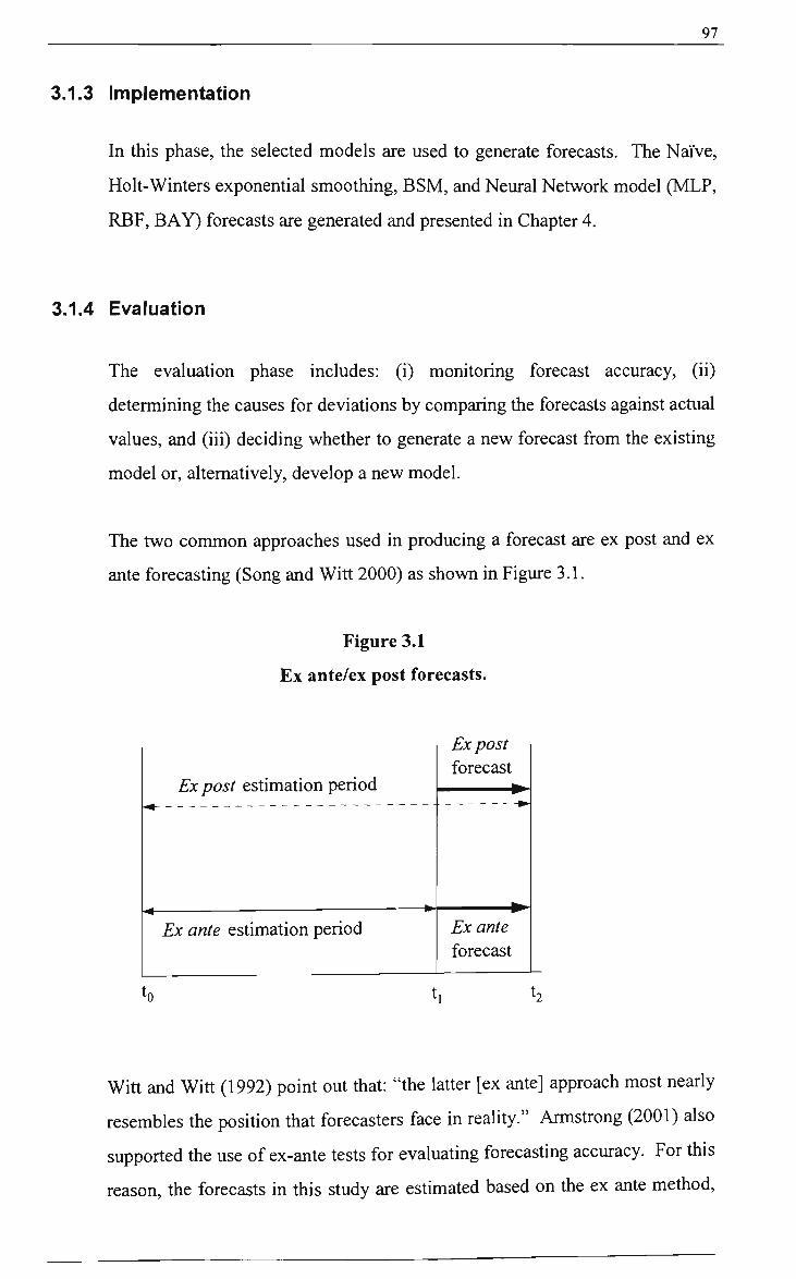
97
3.1.3 Implementation
In this phase, the selected models are used to generate forecasts. The Naive,
Holt-Winters exponential smoothing, BSM, and Neural Network model (MLP,
RBF, BAY) forecasts are generated and presented in Chapter 4.
3.1.4 Evaluation
The evaluation phase includes: (i) monitoring forecast accuracy, (ii)
determining the causes for deviations by comparing the forecasts against actual
values, and (iii) deciding whether to generate a new forecast from the existing
model or, alternatively, develop a new model.
The two common approaches used in producing a forecast are ex post and ex
ante forecasting (Song and Witt 2000) as shown in Figure 3.1.
Figure 3.1
Ex ante/ex post forecasts.
Ex post estimation period
Ex ante estimation period
Ex post forecast
Ex ante forecast
Witt and Witt (1992) point out tiiat: "the latter [ex ante] approach most nearly
resembles tiie position tiiat forecasters face in reality." Armstrong (2001) also
supported the use of ex-ante tests for evaluating forecasting accuracy. For tiiis
reason, the forecasts in this sttidy are estimated based on the ex ante method.

__^ 98
with the estimation period 1985 Quarter 1 to 1999 Quarter 4 and the forecast
period 2000 Quarter 1 to 2001 Quarter 4. A single 'best forecast' model for
each origin-Singapore pair is therefore chosen on the basis of minimum
forecast error. The choice of which is discussed in Chapter 4.
The forecasting horizon has been selected, as discussed before, to be short-
term. Therefore, the performance of the models is compared for only two years
ahead (8 quarters). In order to test the capacity of the forecast models fiilly,
direct forecasts for the whole two years ahead are compared against the shorter
time frames of one quarter ahead per forecast and one year ahead forecasts (4
quarters).
The next chapter discusses the implementation and evaluation of the selected time
series forecasting models for each disaggregated quarterly tourist flow from the six
major tourist generating markets to Singapore (Austtalia, China, India, Japan, UK, and
USA) using the Winters, BSM and Neural Network models. The empirical results and
the findings obtained are presented and discussed.

99
CHAPTER 4 EMPIRICAL RESULTS
Introduction
This chapter presents the empirical results of the time-series forecasting performance
analysis compared on the basis of the selected forecasting performance measures.
Firstly, the various forecasting performance measures are discussed. Next, forecasting
results obtained from each of the forecasting models are given.
4.1 Forecasting Performance Evaluation
While the cost of forecasting must be balanced against the accuracy obtained, the most
important forecast performance criterion is the accuracy of the prediction that is
generated by the forecasting method or model as compared to the actual observation.
As highlighted by Klein (1984), "the forecast ... accuracy is the bottom line for the
professional forecaster". Carbone and Armstrong (1982) also concluded that
forecasting accuracy is the most important forecasting performance criterion, relative
to other criteria such as ease of interpretation, cost/time, and ease of
use/implementation. In another survey by Witt and Witt (1992) carried out at the
'Tourism in the 1990s" conference held in London in November 1986, the results
found that 'accuracy' is the most important forecast performance evaluation criterion.
More recentiy, Yokum and Armsttong (1995) summarised the selection criteria for
selecting a forecasting method that had been examined in earlier surveys by Carbone
and Armstrong (1982), Mahmoud et al. (1986), Mentzer and Cox (1984) and Sanders
and Mandrodt (1994), and found that forecasting accuracy is still the most important
criteria.

100
4.1.1 Forecasting Accuracy Measures
The various types of forecasting accuracy measures (Mahmoud, 1984; Mahmoud,
1990) include: (a) Mean absolute deviation (MAD) or mean absolute error (MAE)
which is the average of the absolute values of the forecast errors with all errors
assigned equal weights, (b) Mean square error (MSE) where large errors are given
additional weight, (c) Root mean squared error (RMSE) which is the square root of
the average of the squared values of the errors, (d) Mean absolute percentage error
(MAPE) which is the average of the absolute values of the percentage errors. These
four common measures each have advantages and limitations (Makridakis 1983;
Makridakis et al. 1998) and are shovm mathematically in Table 4.1 where Ct is the
forecast error in period t (i.e.. Ft - At), At is the actual observation at time t, and Ft
denotes the forecast at time t.
Table 4.1
Forecasting Error Measures
MAD
MSE
MAPE
RMSE
1/n i 1 e, 1 t = i
1/n Z (e,) ' t = i
n
1/n I 1 e, / A, 1 . 100 t= 1
V MSE
However, Makridakis et al. (1983) highlighted that, 'one of the difficulties in dealing
witii the criterion of accuracy in forecasting situations is the absence of a single
universally accepted measure of accuracy'. From a theoretical standpoint, the best
accuracy measure must be robust from one situation to another and not be unduly
influenced by outliers. From a practical point of view, it must make sense, be easily
understood, and convey as much information about accuracy (or errors) as possible.

10]_
Witt and Witt (1992) summarises the use of the various forecasting accuracy measures
used by researchers tiiat include MAD, MSE, RMSE, MAPE and concluded: 'tiiere
are two clear winners: MAPE and RMSE. Many of tiie authors do not discuss tiie
measures that they use but simply employ them'. Additionally:
"The MAPE ... First, being less affected than squared measures by exfreme
errors, it becomes a good relative measure for comparison among techniques.
Secondly, is independent of scale, enabling a comparison to be made between
different time series" (Lawrence et al. 1985, p. 28),
"MAPE being a relative dimensionless measure incorporates the best
characteristics among the various accuracy criteria" (Makridakis 1993, p. 527),
"Both [MAPE and RMSE] of these accuracy criteria are measured in unit-free
terms; they are independent of scale, and hence it is possible to compare data
series of tourist flows which are of widely differing sizes or stated in different
units" (Witt et al. 1992, p. 37).
However, Armsttong (2001) highlighted that given RMSE is based on squaring
forecast errors, it is unreliable, especially if the data contains mistakes or outliers, and
it should not be used for comparison across series. While Carbone and Armsttong
(1982) found that RMSE was the most popular in their survey in 1981, Mentzer and
Kahn (1995) in contrast over a decade later found that MAPE has become the most
commonly used measure (52%) while only 10% used RMSE. The unreliability of
RMSE as a forecasting measure is also highlighted in the findings of Armstrong and
Collopy (1992).
As the disaggregated tourist flow volumes vary considerably among the different
purpose of visits (Holiday, Business and Total) for a given origin country, it is
necessary to use a unit-free measure for comparing forecasting accuracy. The use of
unit-independent measures allows forecasting comparison not only between models
but also across countiies (units) as highlighted by Song and Witt (2001). Hence,
MAPE is selected for forecasting accuracy comparison purposes in tiiis study.

102
4.2 Forecasting Implementation and Evaluation
This section discusses the forecasting implementation and evaluation for the selected
Naive model. Holt-Winters exponential smoothing model, Basic stmctural model, and
tiie MLP, RBF, and BAYN Neural Network models. A summary of tiie forecasting
framework for the selected forecasting models is given in Table 4.2. This table
captures the various issues in the forecasting process as discussed in Chapter 3.
Table 4.2
Forecasting Framework
Data Series
Origin Countries
Forecasting Models
Estimation Period
Post-estimation period
Forecasting Horizon
Forecast Accuracy Measure
Quarterly Holiday, Business and Total Tourist Arrivals into
Singapore
Australia, US, UK, Japan, China and India
Naive, Winters, BSM, Neural Networks (MLP, RBF, BAYN)
1985Q1 to 1999Q4
2000Qlto2001Q4
Direct 8 quarter forecasts. One-quarter ahead forecast. Four-
quarter ahead forecast
MAPE
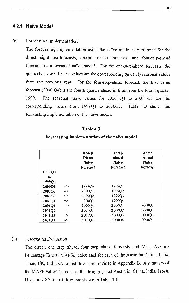
103
4.2.1 Naive Model
(a) Forecasting Implementation
The forecasting implementation using the naive model is performed for the
direct eight-step-forecasts, one-step-ahead forecasts, and four-step-ahead
forecasts as a seasonal naive model. For the one-step-ahead forecasts, the
quarterly seasonal naive values are the corresponding quarterly seasonal values
from the previous year. For the four-step-ahead forecast, the first value
forecast (2000 Q4) is the fourth quarter ahead in time from the fourth quarter
1999. The seasonal naive values for 2000 Q4 to 2001 Q3 are the
corresponding values from 1999Q4 to 2000Q3. Table 4.3 shows the
forecasting implementation of the naive model.
Table 4.3
Forecasting implementation of the naive model
1985 QI to
1999Q4 2000Q1 2000Q2 2000Q3 2000Q4 2001 QI 2001Q2 2001Q3 2001Q4
=> => => => => => => =>
8 Step Direct Naive
Forecast
1999Q4 2000Q1 2000Q2 2000Q3 2000Q4 2001Q1 2001Q2 2001Q3
1 step ahead Naive
Forecast
1999Q1 1999Q2 1999Q3 1999Q4 2000Q1 2000Q2 2000Q3 2000Q4
4 step Ahead Naive
Forecast
2000Q1 2000Q2 2000Q3 2000Q4
(b) Forecasting Evaluation
The direct, one step ahead, four step ahead forecasts and Mean Average
Percentage Errors (MAPEs) calculated for each of the Australia, China, India,
Japan, UK, and USA tourist flows are provided in Appendix B. A summary of
the MAPE values for each of the disaggregated Australia, China, India, Japan,
UK, and USA tourist flows are shown in Table 4.4.

104
Table 4.4
Summary of Naive Forecast MAPEs
Aus Holiday
Aus Business
Aus Total
Average
China Holiday
China Business
China Total
Average
India Holiday
India Business
India Total
Average
Japan Holiday
Japan Business
Japan Total
Average
UK Holiday
UK Business
UK Total
Average
USA Holiday
USA Business
USA Total
Average
Overall
Overall Average 13.15%
Direct forecast 10.45%
11.83%
10.30%
10.86%
12.11%
13.90%
16.04%
14.02%
18.67%
14.97%
13.32%
15.65%
14.97%
12.80%
13.29%
13.69%
11.10%
9.28%
9.14%
9.84%
10.94%
17.40%
10.24%
12.86%
12.82%
1-Step-ahead 9.26%
10.82%
9.13%
9.74%
9.94%
11.50%
13.32%
11.59%
15.18%
12.32%
11.23%
12.91%
25.97%
14.54%
19.95%
20.15%
9.63%
9.20%
8.23%
9.02%
11.58%
20.52%
11.32%
14.47%
12.98%
4-Step-ahead 8.74%
8.87%
9.55%
9.05%
9.98%
3.75%
12.31%
8.68%
7.94%
4.97%
6.33%
6.41%
44.98%
18.13%
32.46%
31.86%
7.11%
8.42%
6.65%
7.39%
13.64%
28.04%
13.79%
18.49%
13.65%

105
4.2.2 Winters Forecasting
(a) Forecasting Implementation
The forecasting implementation using the Holt-Winters exponential smootiiing
model is performed for the direct eight-step-forecasts, one-step-ahead
forecasts, and four-step-ahead forecasts as shovm in Table 4.5.
Table 4.5
Forecasting implementation of the Winters model
Actual
1985 QI to
1999Q4 2000Q1 2000Q2 2000Q3 2000Q4 2001Q1 2001Q2 2001Q3 2001Q4
=> => => => => => => =>
8 Step Direct
Winters Forecast
T Model Estimation
i 1999Q4 2000Q1 2000Q2 2000Q3 2000Q4 2001Q1 2001Q2 2001Q3
1 step ahead
Winters Forecast
T Model Estimation
i 2000Q2 2000Q3 2000Q4 2001Q1 2001Q2 2001Q3 2001Q4
4 step ahead
Winters Forecast
2001Q1 2001Q2 2001Q3 2001Q4
Table 4.6 presents the empirical results for one example of a one-step-ahead
forecast of the Winters Model - Holiday flow forecast from UK to Singapore.
In here, the number of Holiday arrivals from the UK in the 62" Quarter
(2001Q2) is generated, the value being 45961.
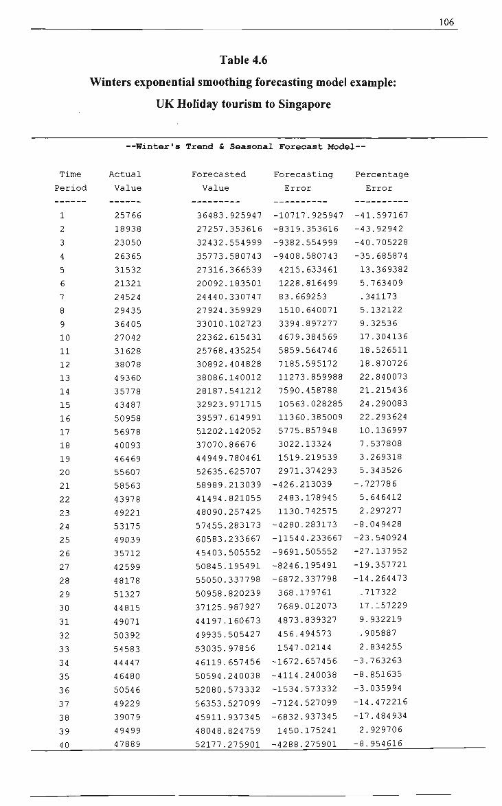
106
Table 4.6
Winters exponential smoothing forecasting model example:
UK Holiday tourism to Singapore
—Winter's Trend & Seasonal Forecast Model—
Time
Period
1
2
3
4
5
6
7
8
9
10
11
12
13
14
15
16
17
18
19
20
21
22
23
24
25
26
27
28
29
30
31
32
33
34
35
36
37
38
39
40
Actual
Value
25766
18938
23050
26365
31532
21321
24524
29435
36405
27042
31628
38078
49360
35778
43487
50958
56978
40093
46469
55607
58563
43978
49221
53175
49039
35712
42599
48178
51327
44815
49071
50392
54583
44447
46480
50546
49229
39079
49499
47889
Forecasted
Value
36483
27257
32432
35773
27316
20092
24440
27924
33010
22362
25768
30892
38086,
28187,
32923,
39597,
51202,
37070,
44949.
52635.
58989.
41494.
48090.
57455.
60583.
45403.
50845.
55050.
50958.
37125.
44197.
49935.
53035.
46119.
50594.
52080.
56353.
45911.
48048.
52177.
.925947
.353616
.554999
.580743
.366539
.183501
.330747
.359929
.102723
.615431
.435254
.404828
.140012
.541212
.971715
.614991
.142052
.86676
.780461
.625707
.213039
.821055
.257425
,283173
,233667
,505552
,195491
,337798
.820239
987927
160673
505427
97856
657456
240038
573332
527099
937345
824759
275901
Forecasting
Error
-10717.925947
-8319.353616
-9382.554999
-9408.580743
4215.633461
1228.816499
83.669253
1510.640071
3394.897277
4679.384569
5859.564746
7185.595172
11273.859988
7590.458788
10563.028285
11360.385009
5775.857948
3022.13324
1519.219539
2971.374293
-426.213039
2483.178945
1130.742575
-4280.283173
-11544.233667
-9691.505552
-8246.195491
-6872.337798
368.179761
7689.012073
4873.839327
456.494573
1547.02144
-1672.657456
-4114.240038
-1534.573332
-7124.527099
-6832.937345
1450.175241
-4288.275901
Percentage
Error
-41.597167
-43.92942
-40.705228
-35.685874
13.369382
5.763409
.341173
5.132122
9.32536
17.304136
18.526511
18.870726
22.840073
21.215436
24.290083
22.293624
10.136997
7.537808
3.269318
5.343526
-.727786
5.646412
2.297277
-8.049428
-23.540924
-27.137952
-19.357721
-14.264473
.717322
17.157229
9.932219
.905887
2.834255
-3.763263
-8.851635
-3.035994
-14.472216
-17.484934
2.929706
-8.954616
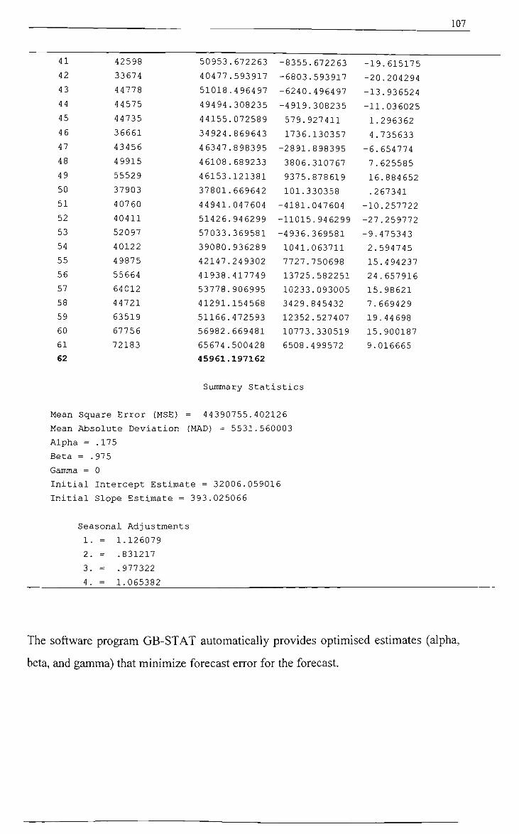
107
41
42
43
44
45
46
47
48
49
50
51
52
53
54
55
56
57
58
59
60
61
62
42598
33674
44778
44575
44735
36661
43456
49915
55529
37903
40760
40411
52097
40122
49875
55664
64012
44721
63519
67756
72183
50953
40477
51018
49494
44155
34924
46347
46108
46153,
37801,
44941,
51426.
57033.
39080.
42147.
41938.
53778.
41291.
51166.
56982.
65674.
45961.
.672263
.593917
.496497
.308235
.072589
.869643
.898395
.689233
.121381
.669642
.047604
.946299
.369581
,936289
,249302
,417749
906995
154568
472593
669481
500428
197162
-8355.672263
-6803.593917
-6240.496497
-4919.308235
579.927411
1736.130357
-2891.898395
3806.310767
9375.878619
101.330358
-4181.047604
-11015.946299
-4936.369581
1041.063711
7727.750698
13725.582251
10233.093005
3429.845432
12352.527407
10773.330519
6508.499572
-19.615175
-20.204294
-13.936524
-11.036025
1.296362
4.735633
-6.654774
7.625585
16.884652
.267341
-10.257722
-27.259772
-9.475343
2.594745
15.494237
24.657916
15.98621
7.669429
19.44698
15.900187
9.016665
Summary Statistics
Mean Square Error (MSE) = 44390755.402126
Mean Absolute Deviation (MAD) = 5531.560003
Alpha = .175
Beta = .975
Gamma = 0
Initial Intercept Estimate = 32006.059016
Initial Slope Estimate = 393.025066
Seasonal Adjustments
1. = 1.126079
2. = .831217
3. = .977322
4. = 1.065382
The software program GB-STAT automatically provides optimised estimates (alpha,
beta, and gamma) that minimize forecast error for the forecast.

108
(b) Forecasting Evaluation
The forecasts and the Mean Average Percentage Errors (MAPEs) are then
calculated for each of the Ausfralia, China, India, Japan, UK, and USA tourist
flows and are presented in Appendix C. A summary of the MAPEs for the
Australia, China, India, Japan, UK, and USA tourist flows is shovm in Table
4.7.
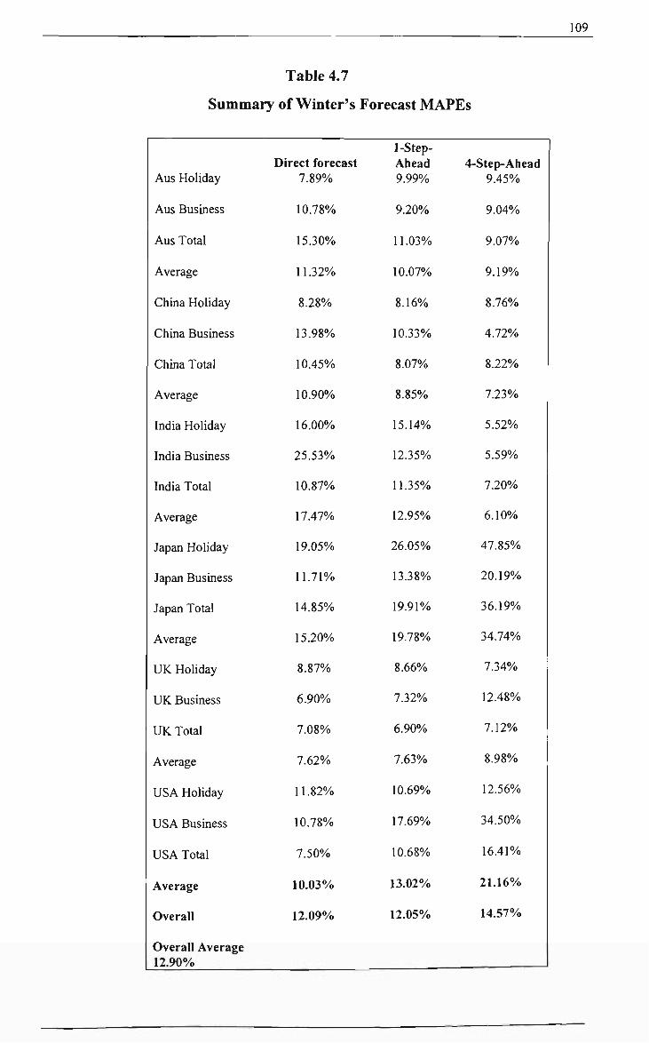
109
Table 4.7
Summary of Winter's Forecast MAPEs
Aus Holiday
Aus Business
Aus Total
Average
China Holiday
China Business
China Total
Average
India Holiday
India Business
India Total
Average
Japan Holiday
Japan Business
Japan Total
Average
UK Holiday
UK Business
UK Total
Average
USA Holiday
USA Business
USA Total
Average
Overall
Overall Average 12.90%
Direct forecast 7.89%
10.78%
15.30%
11.32%
8.28%
13.98%
10.45%
10.90%
16.00%
25.53%
10.87%
17.47%
19.05%
11.71%
14.85%
15.20%
8.87%
6.90%
7.08%
7.62%
11.82%
10.78%
7.50%
10.03%
12.09%
1-Step-Ahead 9.99%
9.20%
11.03%
10.07%
8.16%
10.33%
8.07%
8.85%
15.14%
12.35%
11.35%
12.95%
26.05%
13.38%
19.91%
19.78%
8.66%
7.32%
6.90%
7.63%
10.69%
17.69%
10.68%
13.02%
12.05%
4-Step-Ahead 9.45%
9.04%
9.07%
9.19%
8.76%
4.72%
8.22%
7.23%
5.52%
5.59%
7.20%
6.10%
47.85%
20.19%
36.19%
34.74%
7.34%
12.48%
7.12%
8.98%
12.56%
34.50%
16.41%
21.16%
14.57%
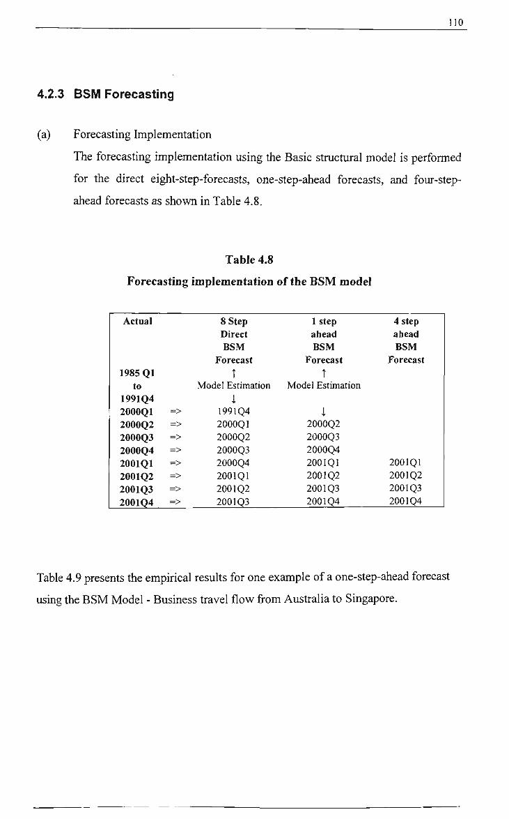
110
4.2.3 BSM Forecasting
(a) Forecasting Implementation
The forecasting implementation using the Basic structural model is performed
for the direct eight-step-forecasts, one-step-ahead forecasts, and four-step-
ahead forecasts as shovm in Table 4.8.
Table 4.8
Forecasting implementation of the BSM model
Actual
1985 QI to
1991Q4 2000Q1 2000Q2 2000Q3 2000Q4 2001Q1 2001Q2 2001Q3 2001Q4
=> => => => => => => =>
8 Step Direct BSM
Forecast t
Model Estimation
i 1991Q4 2000Q1 2000Q2 2000Q3 2000Q4 2001Q1 2001Q2 2001Q3
1 step ahead BSM
Forecast t
Model Estimation
i 2000Q2 2000Q3 2000Q4 2001Q1 2001Q2 2001Q3 2001Q4
4 step ahead BSM
Forecast
2001Q1 2001Q2 2001Q3 2001Q4
Table 4.9 presents the empirical results for one example of a one-step-ahead forecast
using the BSM Model - Business travel flow from Ausfralia to Singapore.
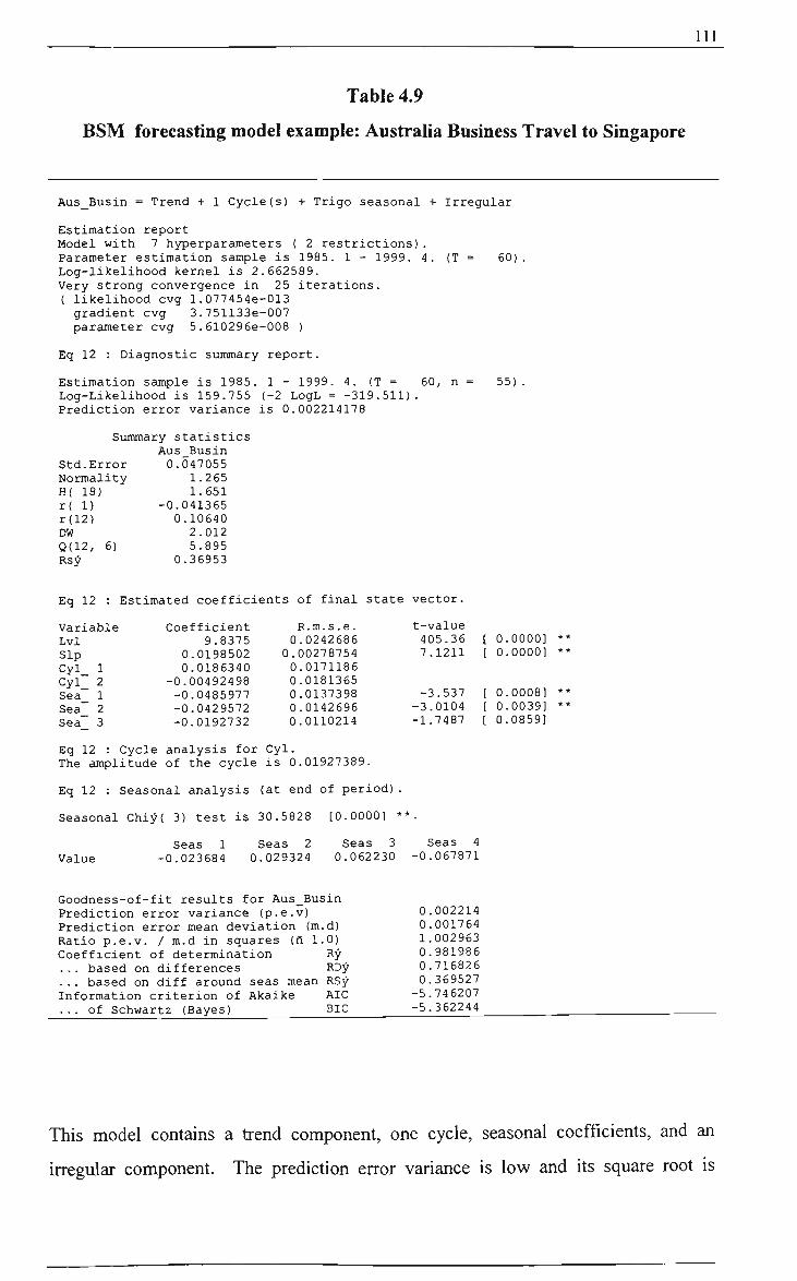
I l l
Table 4.9
BSM forecasting model example: Australia Business Travel to Singapore
Aus_Busin = Trenci + 1 Cycle(s) + Trigo seasonal + Irregular
Estimation report Model with 7 hyperparameters ( 2 restrictions). Parameter estimation sample is 1985. 1 - 1999. 4. {T = 60). Log-likelihooci )cernel is 2.662589. Very strong convergence in 25 iterations. ( likelihood cvg 1.077454e-013 gradient cvg 3.751133e-007 parameter cvg 5.610295e-008 )
Eq 12 : Diagnostic summary report.
Estimation sample is 1985. 1 - 1999. 4. (T = 60, n = 55). Log-Likelihood is 159.755 (-2 LogL = -319.511). Prediction error variance is 0.002214178
Summary statistics
Std.Error Normality H( 18) r( 1) r(12) DW Q(12, 6) Rsy
Aus Busin 0.047055
1.265 1.651
-0.041365 0.10640 2.012 5.895
0.36953
Eq 12 : Estimated coefficients of final state vector.
Variable Lvl Sip Cyl 1 Cyl 2 Sea 1 Sea 2 Sea 3
Coefficient 9.8375
0.0198502 0.0186340
-0.00492498 -0.0485977 -0.0429572 -0.0192732
R.m.s.e. 0.0242686 0.00278754 0.0171186 0.0181365 0.0137398 0.0142696 0.0110214
t-value 405.36 7.1211
-3.537 -3.0104 -1.7487
[ [
[ [ [
0, 0,
0. 0, 0.
.0000]
.0000]
.0008]
.0039]
.0859]
Eq 12 : Cycle analysis for Cyl.
The amplitude of the cycle is 0.01927389.
Eq 12 : Seasonal analysis (at end of period).
Seasonal Chiy{ 3) test is 30.5828 [0.0000] **.
Value Seas 1 Seas 2 Seas 3 Seas 4
-0.023684 0.029324 0.062230 -0.067871
Goodness-of-fit results for Aus_Busin Prediction error variance (p.e.v) Prediction error mean deviation (m.d) Ratio p.e.v. / m.d in squares (n 1.0) Coefficient of determination Ry
based on differences RDy based on diff around seas mean RSy
AIC BIC
Information criterion of Akaike ... of Schwartz (Bayes)
0.002214 0.001764 1.002963 0.981986 0.716826 0.369527 -5.746207 -5.362244
This model contains a frend component, one cycle, seasonal coefficients, and an
irregular component. The prediction error variance is low and its square root is
n2_
presented as tiie "Std Error". The normality test statistic is tiie Bowman-Shenton
statistic based on third and fourth moments of the residuals, with a Chi-square
distribution and 2 degrees of freedom. The critical 5% value is 5.99 and needs to be
exceeded to consider rejecting the model.
H is the heteroskedasticity test statistic, treated as having an F distiibution with 18, 18
degrees of freedom in this example (critical 5% value is 2.23). A low 'H' value
indicates a decrease in variance over time and a high value indicates an increase. The r
values give tiie autocorrelations at given lags. The DW statistic is the standard Durbin
Watson test, and Q is the Box-Ljung statistic based here on 12 autocorrelations, tested
against the Chi-square distribution with six degrees of freedom in this example
(critical 5% value is 12.59). The Rsy statistic compares the model fit against a
random walk with fixed seasonal dummies and as such is a measure of goodness of
fit.
In the final state vector, the t value is the coefficient divided by the root mean square
error, with 1.96 the critical value for 5% statistical significance. The seasonal effects
are jointly tested for significance and the resulting statistic is denoted "Seasonal
Chiy". The probability value is the probability of a Chi-square at s=3, exceeding the
value of the test statistic. The seasonal effect is highly significant here. The final
estimate of the seasonal effect for each season is also provided.
The goodness-of-fit relates to the generalised least squares residuals. The prediction
error variance (p.e.v.) is the variance of the residuals, and the mean deviation of the
residuals is also given. The ratio of the p.e.v. and m.d. should approximate unity in a
correctly specified model. Ry is the equivalent of a regression R square, and RDy
should not be negative. Model comparison are best made using the AIC and BIC
statistics; the lower the value the better the model.
(b) Forecasting Evaluation

113
The forecasts and the Mean Average Percentage Errors (MAPEs) are then
calculated for each of the Australia, China, India, Japan, UK, and USA tourist
flows. A summary of the MAPEs for the Ausfralia, China, India, Japan, UK,
and USA tourist flows is shovm in Table 4.10.
Overall the MAPE is 11.5% for the direct forecast, 8.55% for 1-step-ahead and
9.90% for 4-step-ahead forecasts. The forecasts are good in that they
outperform the naive forecasts and Holt-Winters exponential smoothing
forecasts.

114
Table 4.10
Summary of Basic Structural Model Forecast MAPEs
Aus Holiday
Aus Business
Aus Total
Average
China Holiday
China Business
China Total
Average
India Holiday
India Business
India Total
Average
Japan Holiday
Japan Business
Japan Total
Average
UK Holiday
UK Business
UK Total
Average
USA Holiday
USA Business
USA Total
Average
Overall
Overall Average 9.98%
Direct forecast 13.59%
7.28%
15.99%
12.29%
7.18%
8.46%
10.93%
8.86%
17.85%
10.43%
10.96%
13.08%
19.05%
12.20%
16.18%
15.81%
7.93%
5.65%
5.02%
6.20%
13.23%
15.54%
9.51%
12.76%
11.50%
1-Step-Ahead 5.89%
5.77%
11.72%
7.79%
5.56%
5.67%
10.82%
7.35%
12.01%
5.49%
6.92%
8.14%
16.58%
9.57%
14.33%
13.50%
5.56%
4.26%)
5.16%
4.99%
9.66%
10.85%
8.15%
9.55%
8.55%
4-Step-Ahead 6.49%
7.14%
3.58%
5.73%
5.16%
4.03%
6.94%
5.38%
9.03%.
4.95%.
5.04%
6.34%
30.79%.
15.69%
24.37%.
23.62%
4.77%.
6.78%
5.70%
5.75%.
10.70%
16.11%.
10.85%
12.56%
9.90%

115
4.2.4 Neural Network Forecasting
(a) Forecasting Implementation
Given that Neural Networks are universal approximators of fimctions
(Cybenko 1989) one might expect that they could model seasonal pattems.
However, Kolarik and Rudorfer (1994) and Wheelwright and Makridakis
(1985) have found Neural Networks have difficulty modellmg seasonal
pattems. Nelson et al. (1999) tested this issue and established that for time
series with seasonality, the MAPE for Neural Networks based on
deseasonalised data was significantly more accurate than Neural Networks
based on non-deseasonalised data. Further post-hoc testing was also
performed to establish that this finding was valid across the functional form,
the number of historical data points and the type of forecasting horizon. These
results suggest deseasonalising may benefit forecast accuracy just as with
statistical methods. Consequently, a test is conducted here whereby the results
are given for both a seasonal and deseasonalised series.
Neural models can have two leaming methods 'supervised' and
'unsupervised'. Only a supervised method can be used for time-series analysis
where 'targets' (actual values) can be used to frain the models. An
'unsupervised' model has an intemal comparison process between sets of data
and is best used for clustering analysis. In SPSS the Kohonen Network is
provided as an 'unsupervised' model and is not used here. The three models
MLP, RBF and Bayesian are 'supervised' models suitable for forecasting.
There are also two directions of flow that the leaming process can take
'forward' and 'backward'. Forward flow passes from one node to the next
with information sent only from the preceding node to adjust tiie layer
calculations. Backward flow receives preceding information and compares it
v^th the output before adjusting the layer calculations.
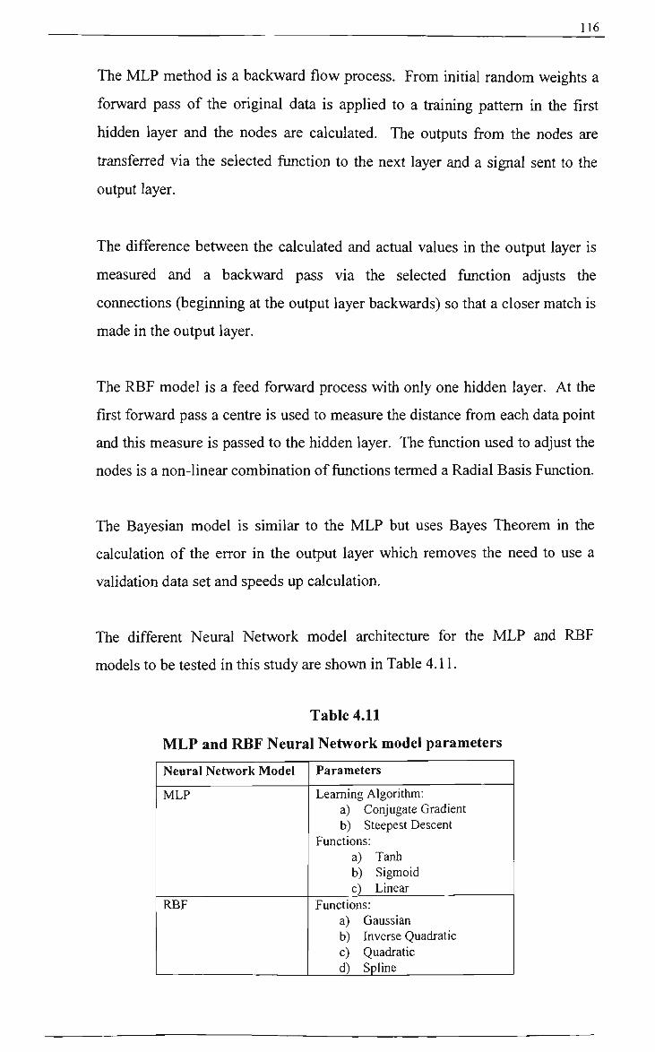
116
The MLP method is a backward flow process. From mitial random weights a
forward pass of the original data is applied to a fraining pattem m tiie first
hidden layer and the nodes are calculated. The outputs from the nodes are
fransferred via the selected fimction to the next layer and a signal sent to the
output layer.
The difference between the calculated and actual values in the output layer is
measured and a backward pass via the selected fimction adjusts the
connections (beginning at the output layer backwards) so that a closer match is
made in the output layer.
The RBF model is a feed forward process with only one hidden layer. At the
first forward pass a centre is used to measure the distance from each data point
and this measure is passed to the hidden layer. The function used to adjust the
nodes is a non-linear combination of functions termed a Radial Basis Function.
The Bayesian model is similar to the MLP but uses Bayes Theorem in the
calculation of the error in the output layer which removes the need to use a
validation data set and speeds up calculation.
The different Neural Network model architecture for the MLP and RBF
models to be tested in this study are shovm in Table 4.11.
Table 4.11
MLP and RBF Neural Network model parameters
Neural Network Model
MLP
RBF
Parameters
Leaming Algorithm: a) Conjugate Gradient b) Steepest Descent
Functions: a) Tanh b) Sigmoid c) Linear
Functions: a) Gaussian b) Inverse Quadratic c) Quadratic d) Spline

117
The resulting Neural Networks models are:
1) MLP conjugate gradient Tanh
2) MLP conjugate gradient Sigmoid
3) MLP conjugate gradient Linear
4) MLP steepest descent Tanh
5) MLP steepest descent Sigmoid
6) MLP steepest descent Linear
7) RBF Gaussian
8) RBF Inverse Quadratic
9) RBF Quadratic
10) RBF Spline
11) Bayesian
The Bayesian Neural Network model has no fimction selection.
Parameter selection is a complex issue. The parameters are largely focussed
upon the number of nodes, the number of hidden layers and difler between the
three network models.
These parameters are best selected by trial and error automatically in the
software and are not reported separately in this study. The reasons for this
need some discussion. For the MLP models the choice of the number of layers
is between one or two, although selecting a second layer often does not
improve forecast accuracy. In the case of this analysis no series was improved
by having more than one layer and this is a finding discussed later. However,
because only one layer was used there is no point in specifying the number of
layers in the model tables.
For tiie MLP the number of nodes in a layer is also selected automatically.
Increasing the number of nodes will improve the accuracy of the MLP model
gradually until 100% fit is achieved on the training data. However, tiiis is

118
because each new unit starts to represent individual features in the data, and it
is possible to over-fit the model and begm to decrease forecasting accuracy
through adding more nodes, as the nodes begin to represent noise in the data.
SPSS uses an automatic convergence criteria to avoid the over-fitting problem.
As such the number of nodes derived is of little practical information and is
not reported.
For the Radial Basis Function model parameter selection focuses upon the
number of cenfres (nodes). Again this is best selected by trial and error
automatically based upon 5 centres as a start mnning up to 50 at intervals of 5.
As with the MLP model the number of centres provides no practical
information when selected automatically and there is no reason to try and
select them manually because of the risk of over-fitting. The positioning of the
centres also needs to be decided and it is possible to select particular data
points such as outliers. However, a reason is needed for doing this, and no
reason exists in this study with this type of data. Consequently, selection is
random through the series as recommended by the SPSS Neural Coimections
software manual.
It needs to be noted that Euclidean error distance was used to calculate the
Radial Basis model because this is the most accurate parameter to use (refer to
the SPSS Neural Connection Manual).
For the Bayesian Network model parameter selection focuses upon the weights
for the parameter groups and given the input data is a time-series
(automatically normalized) of arrivals the paramount basis for deciding is to
reduce noise in the series. This is best done by again selecting an automatic
process (Automatic Relevance Detection) so that the number of groups is
dependent on the number of nodes in the input layer. The number of nodes
selected is also automatic for the same reasons given above for the MLP
model. Also like the MLP model the number of layers could be one or two,
but of the working models, only one layer is selected by the model.

119
A fiirther parameter for the Bayesian model is the number of models. Because
the fraining begins from a randomly selected set of parameter values the
accuracy of calculations (when compared in the output layer) can vary
depending upon the start selected. Consequently it is possible to run several
models with different starting pomts and then have two different decision mles
to select the best model. The choice is Most Likely Models and tiie Committee
Decision. Although initial testing attempted to test the difference m the
decision mles, the Bayesian model did not work for the tune-series in this
study, and mle selection became irrelevant.
The forecasting implementation using the Neural Network model is performed
in two stages for the seasonal data series and deseasonalised data series.
Stage 1: In this stage, each of the eleven Neural Network models as
highlighted above are used to perform the eight-quarter Direct forecast for
each of the disaggregated data series. Appendix B provides the RMSE values
of the MLP and RBF models for the non-deseasonalised data, while Appendix
C provides the RMSE values of the MLP and RBF models for deseasonalised
data. The RMSE forecasting accuracy comparison is used as this error
measure (as conventionally RMSE and not MAPE is used for neural model
selection in the software) to compare across the MLP, RBF, and BAY Neural
Network models with the same data series.
Table 4.12 provides a summary of the best MLP, RBF and Bayesian models
for each deseasonalised data series with their respective RMSE values; the
overall best model is then selected as shovm in the last column. Similarly,
Table 4.13 provides a summary of the best MLP, RBF and Bayesian models
for each non-deseasonalised data series with their respective RMSE values; the
overall best model is then selected as shovm in the last column. The Bayesian
model did not work on the sample data. However, there is no reason as to why
this occurred. In many cases the model could not be calculated at all and when
calculated the model did not provide accurate forecasts.
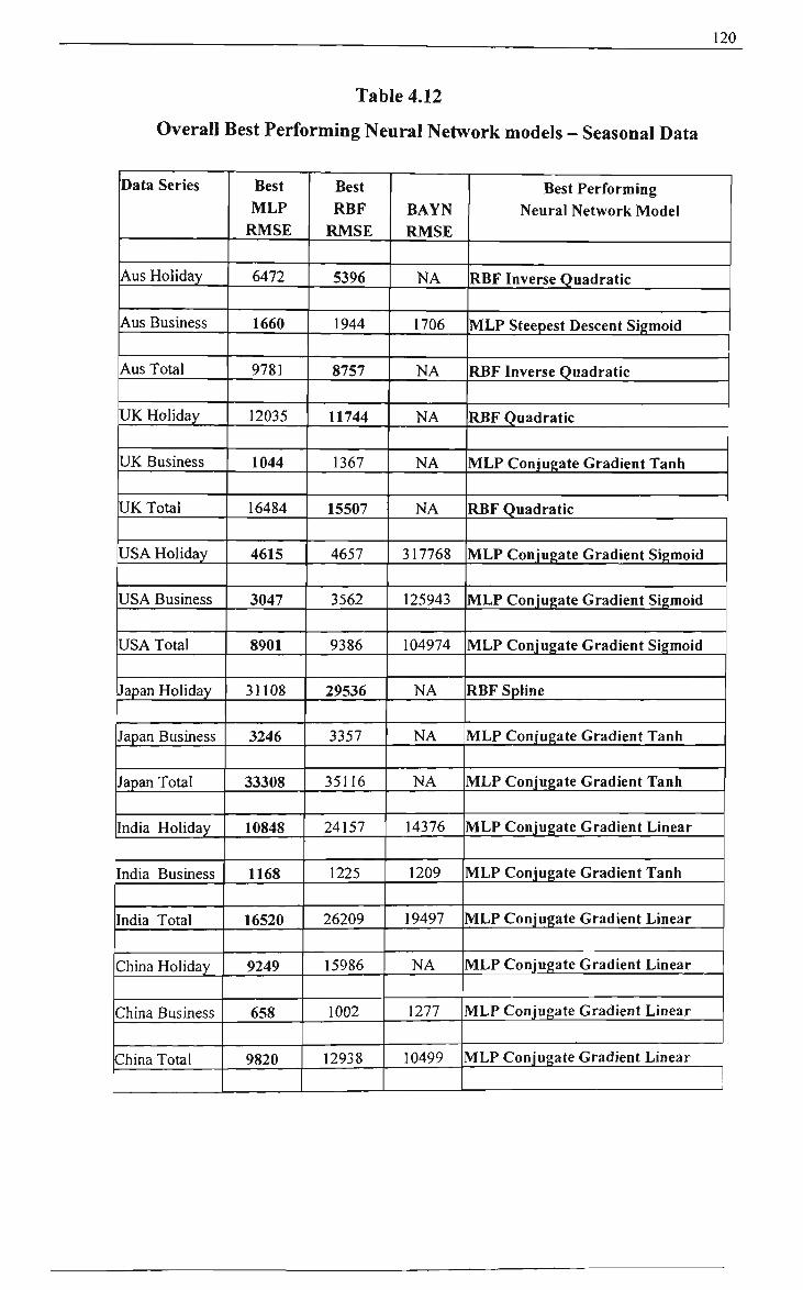
120
Table 4.12
Overall Best Performing Neural Network models - Seasonal Data
Data Series
Aus Holiday
Aus Business
Aus Total
UK Holiday
UK Business
UK Total
USA Holiday
USA Business
USA Total
Japan Holiday
Japan Business
Japan Total
India Holiday
India Business
India Total
China Holiday
China Business
China Total
Best MLP
RMSE
6472
1660
9781
12035
1044
16484
4615
3047
8901
31108
3246
33308
10848
1168
16520
9249
658
9820
Best RBF
RMSE
5396
1944
8757
11744
1367
15507
4657
3562
9386
29536
3357
35116
24157
1225
26209
15986
1002
12938
BAYN RMSE
NA
1706
NA
NA
NA
NA
317768
125943
104974
NA
NA
NA
14376
1209
19497
NA
1277
10499
Best Performing Neural Network Model
RBF Inverse Quadratic
MLP Steepest Descent Sigmoid
RBF Inverse Quadratic
RBF Quadratic
MLP Conjugate Gradient Tanh
RBF Quadratic
MLP Conjugate Gradient Sigmoid
MLP Conjugate Gradient Sigmoid
MLP Conjugate Gradient Sigmoid
RBF Spline
MLP Conjugate Gradient Tanh
MLP Conjugate Gradient Tanh
MLP Conjugate Gradient Linear
MLP Conjugate Gradient Tanh
MLP Conjugate Gradient Linear
MLP Conjugate Gradient Linear
MLP Conjugate Gradient Linear
MLP Conjugate Gradient Linear
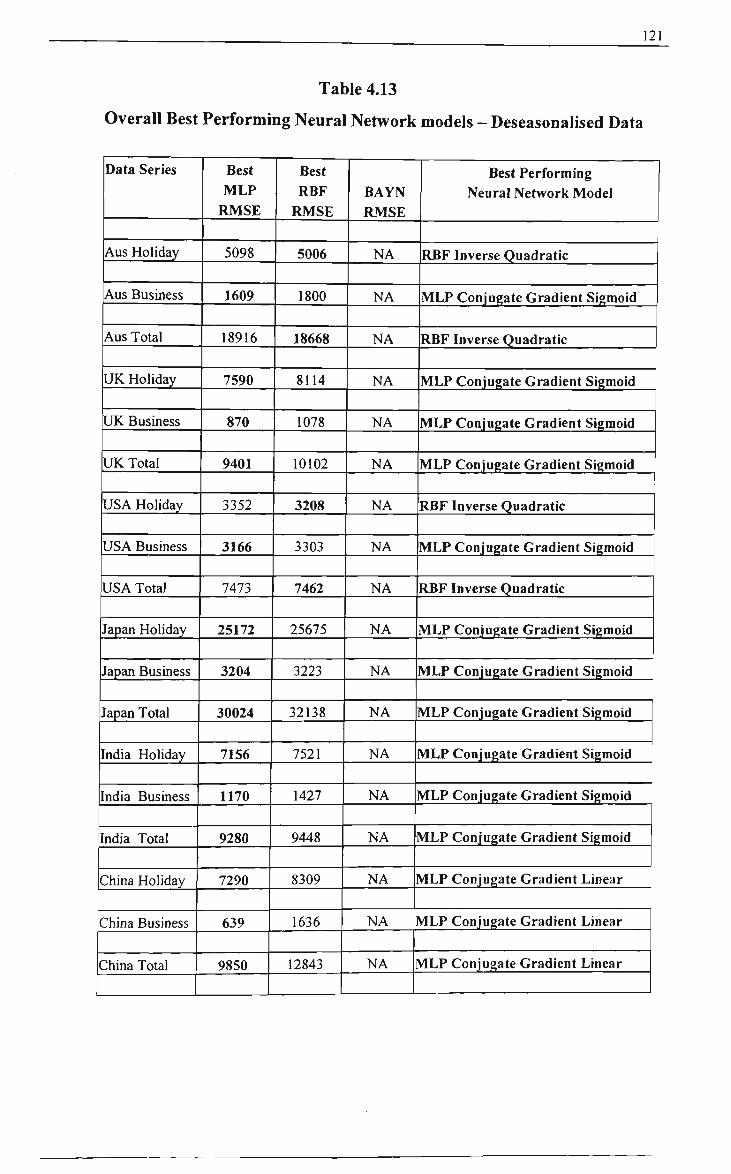
121
Table 4.13
Overall Best Performing Neural Network models - Deseasonalised Data
Data Series
Aus Holiday
Aus Business
Aus Total
UK Holiday
UK Business
UK Total
USA Holiday
USA Business
USA Total
Japan Holiday
Japan Business
Japan Total
India Holiday
India Business
India Total
China Holiday
China Business
Best MLP
RMSE
5098
1609
18916
7590
870
9401
3352
3166
7473
25172
3204
30024
7156
1170
9280
7290
639
China Total 9850
1
Best RBF
RMSE
5006
1800
18668
8114
1078
10102
3208
3303
7462
25675
3223
32138
7521
1427
9448
8309
1636
12843
BAYN RMSE
NA
NA
NA
NA
NA
NA
NA
NA
NA
NA
NA
NA
NA
NA
NA
NA
NA
NA
Best Performing Neural Network Model
RBF Inverse Quadratic
MLP Conjugate Gradient Sigmoid
RBF Inverse Quadratic
MLP Conjugate Gradient Sigmoid
MLP Conjugate Gradient Sigmoid
MLP Conjugate Gradient Sigmoid
RBF Inverse Quadratic
MLP Conjugate Gradient Sigmoid
RBF Inverse Quadratic
MLP Conjugate Gradient Sigmoid
MLP Conjugate Gradient Sigmoid
MLP Conjugate Gradient Sigmoid
MLP Conjugate Gradient Sigmoid
MLP Conjugate Gradient Sigmoid
MLP Conjugate Gradient Sigmoid
MLP Conjugate Gradient Linear
MLP Conjugate Gradient Linear
MLP Conjugate Gradient Linear

122_
Stage 2: Here, the best performing models that were selected from the
seasonalised and deseasonalised tourist data flows from stage 1 are used to
conduct the one-step-ahead forecast and four-step-ahead forecasts. The
multistepping and single-stepping forecasting method used to generate these
forecasts is shovm in Table 4.14.
Table 4.14
Forecasting implementation of the Neural Network models
Actual
1985 QI to
1991Q4 2000Q1 2000Q2 2000Q3 2000Q4 2001 QI 2001Q2 2001Q3 2001Q4
=> => => => => => => =>
8 Step Direct
Neural Network Forecast
(Selected from MLP, RBF,
BAYN models)
t Model Estimation
i 1991Q4 2000Q] 2000Q2 2000Q3 2000Q4 2001Q1 2001Q2 2001Q3
1 step Ahead
Neural Network Forecast
(Using the best Neural Network
model)
T Model Estimation
i 2000Q2* 2000Q3* 2000Q4* 2001Q1* 2001Q2* 2001Q3* 2001Q4*
4 step ahead
Neural Network Forecast
2001 QI* 2001Q2* 2001Q3* 2001Q4*
With Neural Network forecasting, the network is trained over a given training
set and a validation set that is used to evaluate the generalisation capabilities of
the learned model.
A summary of the MAPEs for the Australia, China, India, Japan, UK, and
USA are shown in Table 4.15 and 4.16 for the deseasonalised and seasonal
data series respectively.
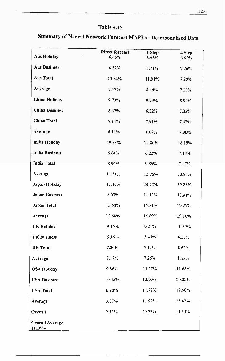
123
Table 4.15
Summary of Neural Network Forecast MAPEs - Deseasonalised Data
Direct forecast 1 Step 4 Step
Aus Holiday 6.46% 6.66% 6.65%
Aus Business 6.52%. 7.71% 7.76%
Aus Total 10.34% 11.01% 7.20%
Average 7.77% 8.46%. 7.20%
China Holiday 9.73% 9.99% 8.94%.
China Business 6.47%. 6.32% 7.32%
China Total 8.14% 7.91% 7.42%
Average 8.11% 8.07% 7.90%
India Holiday 19.33%. 22.80%. 18.19%
India Business 5.64% 6.22% 7.13%
India Total 8.96% 9.86% 7.17%
Average 11.31%. 12.96%. 10.83%
Japan Holiday 17.40%. 20.72% 39.28%
Japan Business 8.07%o 11.13% 18.91%
Japan Total 12.58% 15.81%. 29.27%
Average 12.68%. 15.89%. 29.16%
UK Holiday 9.15%. 9.21% 10.57%
UK Business 5.36% 5.45% 6.37%
UK Total 7.00% 7.13% 8.62%
Average 7.17% 7.26% 8.52%
USA Holiday 9.86%. 11.27%. 11.68%
USA Business 10.45% 12.99%. 20.22%
USA Total 6.90%. 11.72% 17.50%
Average 9.07% 11.99% 16.47%
Overall 9.35% 10.77% 13.34%
Overall Average 11.16%

124

125
Table 4.16
Summary of Neural Network Forecast MAPEs - Seasonal Data
Aus Holiday
Aus Business
Aus Total
Average
China Holiday
China Business
China Total
Average
India Holiday
India Business
India Total
Average
Japan Holiday
Japan Business
Japan Total
Average
UK Holiday
UK Business
UK Total
Average
USA Holiday
USA Business
USA Total
Average
Overall
Overall Average 12.17%
Direct forecast 7.04%
5.83%
4.93%
5.93%
11.55%.
5.80%.
6.84%
8.06%.
22.91%.
6.05%
14.29%
14.42%
22.84%.
8.31%
16.03%
15.73%
13.93%
7.08%
11.17%
10.73%.
14.62%
9.88%
8.16%
10.88%
10.96%.
IStep 6.97%
5.64%
5.38%
6.00%
12.52%,
5.72%.
7.48%
8.57%.
27.89%.
6.79%.
14.41%.
16.36%.
20.24%.
9.01%.
18.20%
15.82%
17.03%.
7.28%
13.26%
12.52%
15.81%
10.33%.
8.43%
11.52%
11.80%
4 Step 6.44%
7.04%
4.45%
5.97%
10.13%
5.60%
7.14%
7.62%
21.94%
4.97%
12.43%
13.11%.
31.33%.
14.01%
24.05%
23.13%.
21.32%
10.05%
16.23%
15.86%
22.56%
15.17%
12.58%
16.77%
13.75%

126
4.3 Forecasting Accuracy Comparison
Table 4.17 shows the forecasting performance accuracy comparisons of the Naive,
Winters, BSM, and Neural Network forecasting methods..
Table 4.17
Forecasting Accuracy Comparison of Naive, Winters,
BSM and Neural Network Models using MAPE
Origin Country
Aus Holiday
Aus Business
Aus Total
Aus Average
China Holiday
Nai've Winters BSM Neural Network -Neural Network -Deseasonalised
Naive Winters BSM Neural Network -Neural Network -Deseasonalised
Naive
Winters BSM Neural Network -Neural Network -Deseasonalised
Naive Winters BSM Neural Network -Neural Network -Deseasonalised
Naive Winters BSM Neural Network -Neural Network -Deseasonalised
- Seasonal
- Seasonal
- Seasonal
Seasonal
• Seasonal
Direct forecast
10.45%. 7.89%o 13.59% 7.04%
6.46%
11.83%. 10.78% 7.28% 5.83%
6.52%.
10.30%
15.30% 15.99% 4.93%
10.34%
10.86%. 11.32%. 12.29%. 5.93%
7.77%
12.11% 8.28% 7.18%, 11.55%
9.73%o
1 Step ahead forecast
9.26% 9.99% 5.89%. 6.97%
6.66%
10.82%. 9.20% 5.77% 5.64%
7.7 P/o
9.13%
11.03%. 11.72% 5.38%
11.01%.
9.74% 10.07%. 7.79% 6.00%,
8.46%
9.94% 8.16% 5.56%, 12.52%.
9.99%
4 Step ahead forecast
8.74%. 9.45%. 6.49% 6.44%
6.65%.
8.87% 9.04% 7.14%. 7.04%
7.76%
9.55%
9.07% 3.58% 4.45%
7.20%
9.05% 9.19% 5.73%, 5.97%.
7.20%
9.98% 8.76% 5.16%, 10.13%.
8.94%.

127
China Business
China Total
China Average
India Holiday
India Business
India Total
India Average
Japan Holiday
Naive Winters BSM Neural Network -Neural Network • Deseasonalised
Naive Winters BSM Neural Network • Neural Network • Deseasonalised
Naive Winters BSM Neural Network -Neural Network -Deseasonalised
Naive Winters BSM Neural Network -Neural Network -Deseasonalised
Naive Winters BSM Neural Network -Neural Network -Deseasonalised
Naive Winters BSM Neural Network -Neural Network -Deseasonalised
Naive Winters BSM Neural Network -Neural Network -Deseasonalised
Naive Winters BSM Neural Network -Neural Network -Deseasonalised
- Seasonal
• Seasonal
• Seasonal
Seasonal
Seasonal
Seasonal
Seasonal
Seasonal
13.90% 13.98% 8.46% 5.80%,
6.47%
16.04% 10.45% 10.93% 6.84%
8.14%
14.02% 10.90% 8.86% 8.06%
8.1 l%o
18.67% 16.00%, 17.85% 22.91%
19.33%
14.97% 25.53% 10.43%, 6.05%
5.64%
13.32% 10.87% 10.96% 14.29%
8.96%
15.65% 17.47% 13.08%. 14.42%
11.31%.
14.97%, 19.05% 19.05% 22.84%.
17.40%.
11.50%. 10.33% 5.67% 5.72%
6.32%
13.32%. 8.07% 10.82% 7.48%,
7.91%,
11.59% 8.85%. 7.35%. 8.57%
8.07%
15.18% 15.14%. 12.01%, 27.89%
22.80%
12.32% 12.35% 5.49%, 6.79%,
6.22%
11.23% 11.35%o 6.92%, 14.41%,
9.86%
12.91%
12.95%, 8.14%. 16.36%
12.96%.
25.97%
26.05%, 16.58%, 20.24%,
20.72%.
3.75%. 4.72% 4.03%, 5.60%
7.32%
12.31% 8.22% 6.94% 7.14%
7.42%
8.68%o 7.23%. 5.38%, 7.62%,
7.90%
7.94%, 5.52% 9.03%.
21.94%
18.19%.
4.97% 5.59%. 4.95%, 4.97%,
7.13%
6.33%o 7.20% 5.04%, 12.43%
7.17%
6.41%,
6.10%, 6.34% 13.1 l%o
10.83%.
44.98%
47.85%. 30.79%, 31.33%
39.28%.

128
Japan Business
Japan Total
Japan Average
UK Holiday
UK Business
UK Total
UK Average
USA Holiday
Naive Winters BSM Neural Network -Neiu-al Network -Deseasonalised
Naive Winters BSM Neural Network -Neural Network -Deseasonalised
Naive Winters BSM Neural Network -Neural Network -Deseasonalised
Naive Winters BSM Neiu-al Network -Neural Network -Deseasonalised
Naive Winters BSM Neural Network -Neural Network -Deseasonalised
Naive Winters BSM Neural Network -Neural Network -Deseasonalised
Naive Winters BSM Neural Network -Neural Network -Deseasonalised
Naive Winters BSM Neural Network -Neural Network -Deseasonalised
Seasonal
Seasonal
Seasonal
Seasonal
Seasonal
Seasonal
Seasonal
Seasonal
12.80% 11.71% 12.20% 8.31%
8.07%,
13.29% 14.85% 16.18% 16.03%
12.58%,
13.69% 15.20% 15.81% 15.73%
12.68%
11.10% 8.87% 7.93%, 13.93%,
9.15%
9.28% 6.90% 5.65% 7.08%o
5.36%,
9.14% 7.08%, 5.02%, 11.17%
7.00%
9.84%
7.62% 6.20%, 10.73%.
7.17%
10.94% 11.82% 13.23%o 14.62%
9.86%
14.54% 13.38% 9.57% 9.01%
11.13%
19.95% 19.91% 14.33% 18.20%
15.81%.
20.15% 19.78% 13.50% 15.82%
15.89%
9.63% 8.66% 5.56% 17.03%.
9.21%
9.20% 7.32%. 4.26%. 7.28%o
5.45%.
8.23%. 6.90% 5.16% 13.26%
7.13%
9.02%.
7.63% 4.99%. 12.52%
7.26%
11.58%
10.69% 9.66%, 15.81%
11.27%
18.13% 20.19%. 15.69% 14.01%,
18.91%
32.46%, 36.19% 24.37% 24.05%.
29.27%,
31.86%,
34.74%, 23.62% 23.13%,
29.16%,
7.11%.
7.34%o 4.77% 21.32%
10.57%
8.42% 12.48% 6.78%. 10.05%
6.37%,
6.65%
7.12% 5.70%, 16.23%
8.62%
7.39%
8.98% 5.75%, 15.86%
8.52%.
13.64%
12.56% 10.70%, 22.56%o
11.68%

129
USA Business
USA Total
USA Average
Overall Average
Overall Average ahead and 4-step Naive Winters BSM Neural Network -Neural Network -
Naive Winters BSM Neural Network -Neural Network -Deseasonalised
Naive Winters BSM Neural Network -Neural Network -Deseasonalised
Naive Winters BSM Neural Network -Neural Network -Deseasonalised
Naive Winters BSM Neural Network Neural Network Deseasonalised
of Direct, 1-step-ahead forecasts:
- Seasonal - Deseasonalised
Seasonal
Seasonal
Seasonal
- Seasonal
13.15%, 12.90%o 9.98%, 12.17%, 11.16%,
17.40% 10.78% 15.54% 9.88%,
10.45%
10.24% 7.50% 9.51% 8.16%
6.90%,
12.86% 10.03% 12.76%, 10.88%
9.07%o
12.82% 12.09%, 11.50%, 10.96%,
1 1 9.35%,
20.52% 17.69% 10.85%, 10.33%,
12.99%,
11.32%, 10.68% 8.15%, 8.43%
11.72%
14.47% 13.02% 9.55% 11.52%
11.99%
12.98%, 12.05%, 8.55%, 11.80%o
10.77%,
28.04% 34.50% 16.11% 15.17%
20.22%
13.79% 16.41% 10.85%, 12.58%
17.50%
18.49%, 21.16%, 12.56%, 16.77%.
16.47%o
13.65%, 14.57%, 9.90%, 13.75%,
13.34%o

130
The followdng findmgs are concluded upon from the empirical results above :
1) Are the modern time series models better than traditional simpler forecasting
Holt-Winters and naifve models?
From Table 4.17, overall average BSM MAPE (9.98%) and Neural Network model
MAPE with deseasonalised data (11.16%) are lower than those for the Holt-Winters
(12.90%) and naive model (13.15%). Based on the MAPE, tiie BSM model is tiie
more accurate model with lowest MAPE value. Statistically, the BSM is significantly
lower (t-3.56, 0.012) at 95% than the naive and Wmters models (t=2.44, 0.035).
However, the deseasonalised Neural Network model MAPE is not sigiuficantly lower
(t=1.67, 0.09) than the naive model, and tiie Winters model (t=1.21, 0.145).
Consequently, the study findings suggest that the Basic structural time series model
and Neural Network model forecast more accurately than the traditional simpler
extrapolative forecasting Holt-Winters and naive models.
2) Do any of the models perform better over different forecasting horizons?
Witii the Direct forecast, it can be seen from Table 4.17, the deseasonalised Neural
Network forecasting model (MAPE 9.35%) outperforms the seasonal Neural Network
model (MAPE 10.96%), BSM (MAPE 11.50%), Winters (MAPE 12.09%), and naive
model (MAPE 12.82%). Statistically, the deseasonalised neural model is significantly
lower (t=2.78, 0.01) at 95% tiian the naive model. However, it is not significantiy
lower than the seasonal Neural Network (t=0.91, 0.19), BSM (t=1.30, 0.11) or
Winters (t=1.59, 0.07) models.
With tiie 1-step-ahead forecasts, the BSM forecasting model (MAPE 8.55%)
outperforms the deseasonalised neural model (MAPE 10.77%), the seasonal neural
model (MAPE 11.80), the Winters (MAPE 12.05%), and tiie naive model (MAPE
12.98%). Statistically, tiie BSM is significantly lower (t=2.19, 0.03) at 95% tiian tiie

131
naive model, but not for the Winters (t=1.64, 0.07), seasonal Neural Network (t=1.61,
0.07) or deseasonalised Neural Network (t=1.23, 0.12) models.
With the 4-step-ahead forecasts, the BSM forecasting model (MAPE 9.90%)
outperforms the deseasonalised Neural Network (MAPE 13.34%), seasonal Neural
Network (MAPE 13.75%), Winters (MAPE 14.57%), and naive model (MAPE
13.65%)). Statistically, the BSM is not significantly lower (t=0.74, 0.24) at 95% than
the naive model. Winters (t=0.85, 0.21), seasonal Neural Network (t=0.98, 0.18) or
deseasonalised Neural Network (t=0.76, 0.23) models.
This overall result suggests that the BSM model is more accurate for forecasting
short-term quarterly tourist flows up to one year ahead than the Neural Network model
or the simpler models. However, for two years ahead the neural model is superior to
tiie BSM model.
3) Did any particular model perform better for different types of tourist flows
(that is. Holiday, Business and Total flows)?
The Holiday, Business, and Total flow overall average MAPEs for tiie Direct, 1-step-
ahead and 4-step-ahead forecast are shovm in Table 4.18,4.19 and 4.20 respectively.
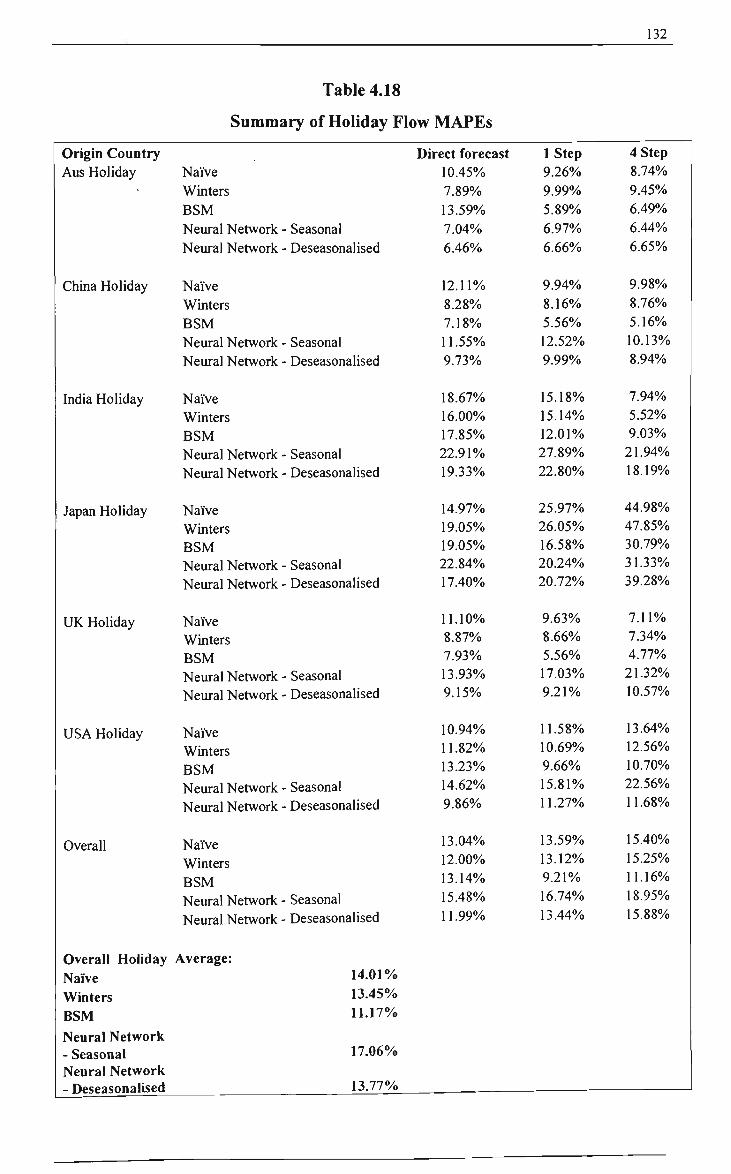
132
Table 4.18
Summary of Holiday Flow MAPEs
Origin Country Aus Holiday
-
China Holiday
India Holiday
Japan Holiday
UK Holiday
USA Holiday
Overall
Naive Winters BSM Neural Network • Neural Network •
Naive Winters BSM Neural Network • Neural Network -
Naive Winters BSM Neitfal Network • Neiu-al Network •
Naive Winters BSM Neural Network -Neural Network -
Naive Winters BSM Neural Network -Neural Network -
Naive Winters BSM Neiffal Network -Neiu-al Network -
Naive Winters BSM Neural Network -Neural Network -
Overall Holiday Average: Naive Winters BSM Neural Network - Seasonal Neural Network - Deseasonalised
• Seasonal • Deseasonalised
• Seasonal • Deseasonalised
• Seasonal • Deseasonalised
• Seasonal • Deseasonalised
• Seasonal • Deseasonalised
• Seasonal • Deseasonalised
Seasonal Deseasonalised
14.01%, 13.45%, 11.17%,
17.06%,
13.77%,
Direct forecast 10.45% 7.89% 13.59% 7.04% 6.46%
12.11% 8.28% 7.18% 11.55% 9.73%
18.67% 16.00% 17.85% 22.91%. 19.33%
14.97% 19.05%. 19.05%. 22.84% 17.40%
11.10% 8.87%, 7.93% 13.93%, 9.15%,
10.94% 11.82% 13.23% 14.62% 9.86%
13.04% 12.00% 13.14% 15.48% 11.99%
IStep 9.26% 9.99% 5.89% 6.97% 6.66%
9.94% 8.16% 5.56% 12.52% 9.99%
15.18%, 15.14% 12.01% 27.89%, 22.80%,
25.97% 26.05%, 16.58% 20.24%, 20.72%,
9.63% 8.66%o 5.56% 17.03% 9.21%,
11.58%
10.69%. 9.66%. 15.81% 11.27%o
13.59%. 13.12%. 9.21% 16.74%. 13.44%.
4 Step 8.74% 9.45%. 6.49% 6.44% 6.65%
9.98% 8.76% 5.16% 10.13% 8.94%
7.94% 5.52% 9.03%.
21.94% 18.19%.
44.98%
47.85% 30.79% 31.33% 39.28%
7.11%
7.34%. 4.77%. 21.32%. 10.57%
13.64%
12.56% 10.70% 22.56% 11.68%.
15.40%.
15.25% 11.16% 18.95%
15.88%
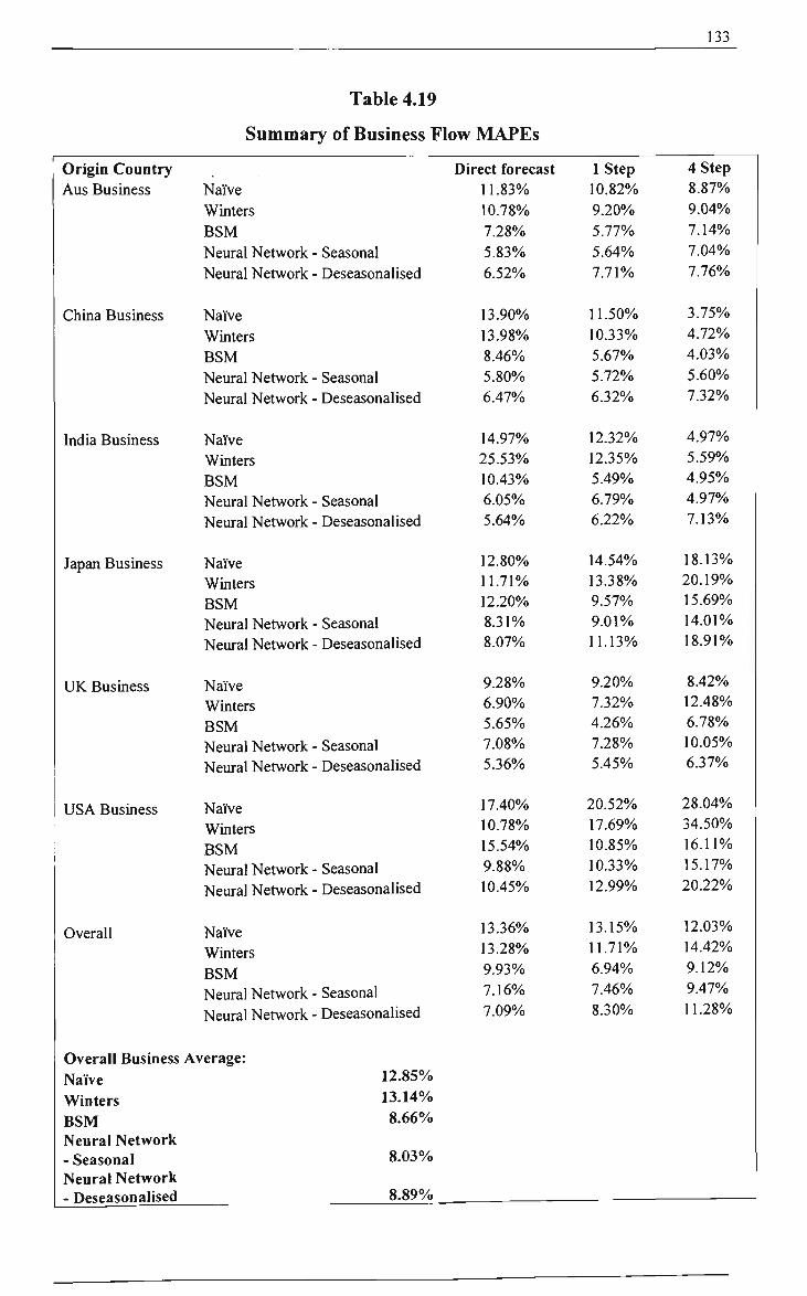
133
Table 4.19
Summary of Business Flow MAPEs
Origin Country Aus Business
China Business
India Business
Japan Business
UK Business
USA Business
Overall
Naive Winters BSM Neural Network • Neural Network •
Naive Winters BSM Neural Network -Neural Network •
Naive Winters BSM Neural Network -Neural Network -
Naive Winters BSM Neural Network • Neural Network •
Naive Winters BSM Neural Network • Neural Network •
Naive Winters BSM Neural Network -Neiu-al Network •
Naive Winters BSM Neural Network -Neural Network -
Overall Business Average: Naive Winters BSM Neural Network - Seasonal Neural Network - Deseasonalised
• Seasonal • Deseasonalised
Seasonal Deseasonalised
• Seasonal • Deseasonalised
• Seasonal • Deseasonalised
• Seasonal • Deseasonalised
• Seasonal • Deseasonalised
Seasonal Deseasonalised
12.85%, 13.14%, 8.66%,
8.03%o
8.89%o
Direct forecast 11.83% 10.78% 7.28% 5.83% 6.52%
13.90% 13.98% 8.46% 5.80%, 6.47%,
14.97% 25.53% 10.43% 6.05% 5.64%
12.80% 11.71% 12.20% 8.31% 8.07%
9.28% 6.90%, 5.65% 7.08%. 5.36%
17.40% 10.78% 15.54% 9.88% 10.45%.
13.36% 13.28%. 9.93% 7.16% 7.09%
IStep 10.82% 9.20%, 5.77% 5.64% 7.71%
11.50% 10.33% 5.67% 5.72% 6.32%
12.32% 12.35% 5.49% 6.79% 6.22%
14.54% 13.38% 9.57%, 9.01%, 11.13%,
9.20%, 7.32% 4.26%, 7.28%, 5.45%,
20.52% 17.69% 10.85% 10.33%, 12.99%
13.15% 11.71% 6.94%, 7.46%. 8.30%.
4 Step 8.87%. 9.04% 7.14% 7.04% 7.76%.
3.75% 4.72% 4.03% 5.60%. 7.32%
4.97%. 5.59% 4.95% 4.97%. 7.13%.
18.13% 20.19%. 15.69% 14.01% 18.91%
8.42% I2.48%o 6.78%. 10.05% 6.37%
28.04%.
34.50%. 16.11%. 15.17%. 20.22%.
12.03%
14.42% 9.12% 9.47% 11.28%
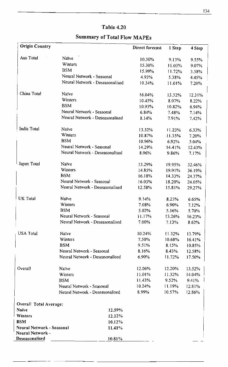
134
Table 4.20
Summary of Total Flow MAPEs
Origin Country
Aus Total
China Total
India Total
Japan Total
UK Total
USA Total
Overall
Naive Winters BSM Neural Network Neural Network
Naive Winters BSM Neural Network Neural Network
NaiVe Winters BSM Neural Network Neural Network
Naive Winters BSM Neural Network • Neural Network •
Naive Winters BSM Nexu*al Network -Neural Network -
Naive Winters BSM Neural Network -Neural Network -
Naive Winters BSM Neural Network -Neural Network -
Overall Total Average: Naive Winters BSM Neural Network -Neural Network -Deseasonalised
Seasonal
- Seasonal - Deseasonalised
- Seasonal - Deseasonalised
- Seasonal - Deseasonalised
- Seasonal • Deseasonalised
Seasonal Deseasonalised
Seasonal Deseasonalised
Seasonal Deseasonalised
12.59%. 12.12%o 10.12%o 11.41%,
10.81%,
Direct forecast
10.30% 15.30% 15.99% 4.93% 10.34%
16.04% 10.45% 10.93% 6.84% 8.14%
13.32% 10.87% 10.96% 14.29%, 8.96%
13.29% 14.85% 16.18% 16.03% 12.58%
9.14% 7.08% 5.02% 11.17% 7.00%,
10.24% 7.50%, 9.51% 8.16% 6.90%
12.06% 11.01% 11.43%, 10.24% 8.99%
IStep
9.13% 11.03% 11.72% 5.38% 11.01%,
13.32% 8.07% 10.82% 7.48% 7.91%
n.23% 11.35% 6.92%, 14.41%o 9.86%,
19.95% 19.91% 14.33% 18.20%, 15.81%,
8.23% 6.90%. 5.16% 13.26%. 7.13%
11.32% 10.68%. 8.15% 8.43% 11.72%
12.20% 11.32%, 9.52%, 11.19% 10.57%.
4 Step
9.55% 9.07% 3.58% 4.45% 7.20%
12.31% 8.22%. 6.94%. 7.14% 7.42%.
6.33% 7.20% 5.04%, 12.43% 7.17%.
32.46% 36.19%, 24.37% 24.05% 29.27%
6.65% 7.12% 5.70% 16.23% 8.62%
13.79% 16.41% 10.85% 12.58% 17.50%
13.52% 14.04% 9.41% 12.81% 12.86%
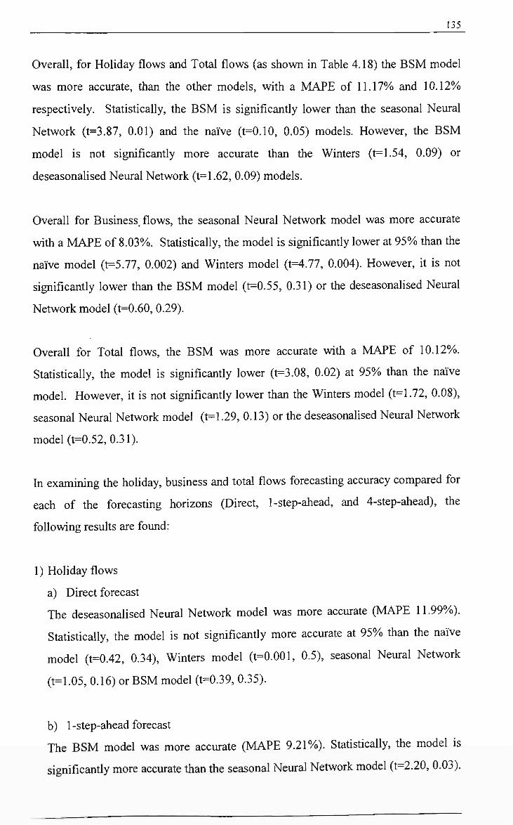
135
Overall, for Holiday flows and Total flows (as shovm in Table 4.18) the BSM model
was more accurate, than the other models, with a MAPE of 11.17% and 10.12%
respectively. Statistically, the BSM is significantly lower than the seasonal Neural
Network (t=3.87, 0.01) and the naive (t=0.10, 0.05) models. However, the BSM
model is not significantly more accurate than the Winters (t=1.54, 0.09) or
deseasonalised Neural Network (t=1.62, 0.09) models.
Overall for Business, flows, the seasonal Neural Network model was more accurate
with a MAPE of 8.03%. Statistically, the model is significantly lower at 95%) tiian tiie
naive model (t=5.77, 0.002) and Winters model (t=4.77, 0.004). However, it is not
significantly lower than the BSM model (t=0.55, 0.31) or the deseasonalised Neural
Network model (t=0.60, 0.29).
Overall for Total flows, the BSM was more accurate wdth a MAPE of 10.12%).
Statistically, tiie model is significantiy lower (t=3.08, 0.02) at 95% tiian tiie naive
model. However, it is not significantly lower than the Winters model (t=1.72, 0.08),
seasonal Neural Network model (t=1.29, 0.13) or tiie deseasonalised Neural Network
model (t=0.52, 0.31).
In examining the holiday, business and total flows forecasting accuracy compared for
each of the forecasting horizons (Direct, 1-step-ahead, and 4-step-ahead), the
following results are found:
1) Holiday flows
a) Direct forecast
The deseasonalised Neural Network model was more accurate (MAPE 11.99%).
Statistically, the model is not significantiy more accurate at 95% tiian tiie naive
model (t=0.42, 0.34), Winters model (t=0.001, 0.5), seasonal Neural Network
(t=1.05, 0.16) or BSM model (t=0.39, 0.35).
b) 1-step-ahead forecast
The BSM model was more accurate (MAPE 9.21%). Statistically, the model is
significantiy more accurate than the seasonal Neural Network model (t=2.20, 0.03).

136
However, it is not significantly more accurate at 95%, than the naive model (t=1.37,
0.1), Winters model (t=1.17, 0.13), or deseasonalised Neural Network model
(t=1.29,0.11).
c) 4-step-ahead forecast
The BSM model was more accurate (MAPE 11.16%). Statistically, the model is not
significantly more accurate at 95% than the naive model (t=0.58, 0.29), Winters
model (t=0.53, 0.30), seasonal Neural Network (t=1.42, 0.09) or deseasonalised
Neural Network model (t=0.74, 0.23).
2) Business flows
d) Direct forecast
The deseasonalised Neural Network model was more accurate (MAPE 7.09%).
Statistically, the model is significantly more accurate at 95% than the naive model
(t=4.57, 0.0005), Winters model (t=2.26, 0.02), BSM model (t=1.71, 0.06), and
seasonal Neural Network (t=0.07, 0.47).
e) 1-step-ahead forecast
The BSM model was more accurate (MAPE 6.94%). Statistically, the model is
sigiuficantly more accurate at 95% than the naive model (t=3.18, 0.01), Winters
model (t=2.60, 0.01), seasonal Neural Network model (t=0.40, 0.35), and
deseasonalised Neural Network model (t=0.83, 0.21).
f) 4-step-ahead forecast
The BSM model was more accurate (MAPE 9.12%). Statistically, the model is not
significantly more accurate at 95%. than the naive model (t=0.66, 0.26), Winters
model (t=1.04, 0.16), seasonal Neural Network model (t=0.13, 0.45), and
deseasonalised Neural Network model (t=0.63, 0.27).
3) Total flows
g) Direct forecast

137
The deseasonalised Neural Network model was more accurate (MAPE 8.99%).
Statistically, the model is significantly more accurate at 95%) than the naive model
(t=2.21, 0.03). However, it is not significantly more accurate than the Winters
model (t=1.20, 0.12), BSM model (t=1.26, 0.12), and seasonal Neural Network
model (t=0.63, 0.27).
h) 1-step-ahead forecast
The BSM model was more accurate (MAPE 9.52%). Statistically, the model is not
significantly more accurate at 95%) than the naive model (t=1.21, 0.13), Winters
model (t=0.78, 0.28), seasonal Neural Network model (t=0.69, 0.25) or
deseasonalised Neural Network model (t=0.56, 0.29).
i) 4-step-ahead forecast
The BSM model was more accurate (MAPE 9.41%). Statistically, the model is not
sigiuficantiy more accurate at 95% than the naive model (t=0.81, 0.22), Winters
model (t=0.82, 0.22), seasonal Neural Network model (t=0.80, 0.22) or
deseasonalised Neural Network model (t=0.71, 0.25).
This suggests that the Neural Networks with deseasonalised data were more accurate
across all flows for the Direct forecasts; while tiie BSM was more accurate across all
flows for the 1-step-ahead and 4-step-ahead forecasts. However, there was no
difference between the different data series disaggregated by purpose of visit in regard
to particular forecasting models.
4) Does disaggregation of the Total flows improve forecast accuracy?
Table 4.21 shows tiie overall average MAPEs for tiie best flows for each type of
travel.
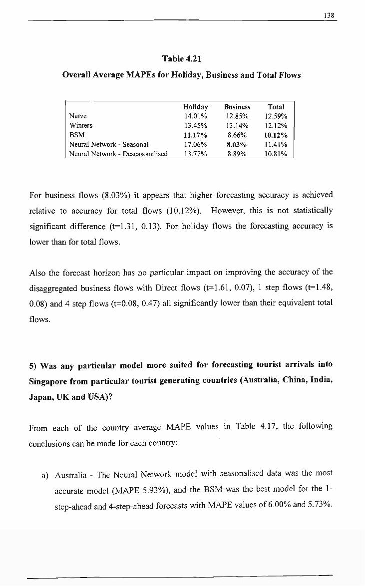
138
Table 4.21
Overall Average MAPEs for Holiday, Business and Total Flows
Naive Winters BSM Neural Network - Seasonal Neural Network - Deseasonalised
Holiday 14.01% 13.45% 11.17% 17.06% 13.77%
Business 12.85% 13.14% 8.66% 8.03%o 8.89%
Total 12.59% 12.12% 10.12%, 11.41% 10.81%
For business flows (8.03%) it appears that higher forecasting accuracy is achieved
relative to accuracy for total flows (10.12%)). However, this is not statistically
significant difference (t=1.31, 0.13). For holiday flows the forecasting accuracy is
lower than for total flows.
Also the forecast horizon has no particular impact on improving the accuracy of the
disaggregated business flows with Direct flows (t=1.61, 0.07), 1 step flows (t=1.48,
0.08) and 4 step flows (t=0.08, 0.47) all significantiy lower than tiiefr equivalent total
flows.
5) Was any particular model more suited for forecasting tourist arrivals into
Singapore from particular tourist generating countries (Australia, China, India,
Japan, UK and USA)?
From each of the countty average MAPE values in Table 4.17, the following
conclusions can be made for each coimtry:
a) Australia - The Neural Network model with seasonalised data was the most
accurate model (MAPE 5.93%), and the BSM was the best model for the 1-
step-ahead and 4-step-ahead forecasts witii MAPE values of 6.00% and 5.73%.

139_
b) China - The Neural Network model with seasonalised data was the most
accurate model (MAPE 8.06%), and the BSM was tiie best model for tiie 1-
step-ahead and 4-step-ahead forecasts witii MAPE values of 7.35% and 5.38%.
c) India - The Neural Network model with deseasonalised data was the most
accurate model (MAPE 11.31%), and the BSM was the best model for the 1-
step-ahead forecasts with a MAPE of 8.14%), while the Holt-Winters was the
best model for the 4-step-ahead forecasts with a MAPE of 6.10%).
d) Japan - The Neural Network model with deseasonalised data was the most
accurate model (MAPE 12.86%), and the BSM was the best model for tiie 1-
step-ahead forecasts with MAPE 13.5%. For the 4-step-ahead forecasts, the
Neural Network model with seasonal data was best model with a MAPE of
23.13%.
e) UK - The BSM was the most accurate model over the three forecasting
horizons with MAPEs of 6.20%, 4.99% and 5.75%) respectively.
f) USA - The Neural Network model with deseasonalised data was the most
accurate model (MAPE 9.07%), and the BSM was the most accurate model for
the 1-step-ahead and 4-step-ahead forecasts with MAPE values of 9.55% and
12.56%.
Only for the UK was the BSM selected as the most accurate model across all the
forecasting horizons. Consequently, there is no evidence of particular models being
suited to particular countries. The overall results for most countries supports the
previous finding that Neural Network models and BSM models are the most accurate
with the Neural Network model working better over longer forecasting horizon and
tiie BSM model working better over a shorter forecasting horizon.

140
6) Did deseasonalising the data improve the forecasting accuracy of the Neural
Network models?
A summary of the Neural Network forecasting performance with seasonal and
deseasonalised data is shovm in Table 4.22.
Table 4,22
Summary of overall average MAPEs for the Neural Network models
with seasonal and deseasonalised data
Neural Network - Seasonal Neural Network - Deseasonalised
Direct forecast
10.96%, 9.35%
1-step-ahead forecast 11.80% 10.77%
4-step-ahead forecast 13.75%, 13.34%,
The results suggests that the Neural Network models using deseasonalised data
perform better than the Neural Network models using seasonal data in all of the three
forecasting horizons examined. However, the differences are not statistically
significant with tiie Direct difference (t=0.92, 0.19), 1 step difference (t=0.47, 0.32)
and 4 step difference (t=0.09, 0.46) all insignificant at 95%.
The conclusion here is that deseasonalising the data improves the forecasting accuracy
of Neural Network models when forecasting seasonal tourism arrivals data. However,
the improvement cannot be said to be statistically significant.
7) Which Neural Network model architecture was most suitable for tourist
arrival forecasting?
From Tables 4.12 and 4.13, it was found tiiat the MLP Conjugate Gradient model was
the best performing Neural Network model for 26 data series out of the 36 seasonal

141
and deseasonalised data series. In particular, the MLP Conjugate Gradient Sigmoid
model was tiie selected as tiie best model for 14 data series. This has been the most
commonly used model in previous tourism forecasting and is found to be the best
defauh model. However, for some series altemative models do improve forecast
accuracy so tiiat just using an MLP Conjugate Gradient model for lower cost will
mean possibly achieving lower accuracy.
8) Do different Neural Network model activation functions have an affect on the
forecasting accuracy of the model?
Appendices B and C give the RMSE values and particular fimctions used for the
different Neural Network models. The RMSE results indicate that different fimctions
are associated with particular Neural Network model architecture and can have a
significant effect on the forecasting performance of the model.
Therefore attention must be given to testing and selecting the most appropriate
functions before applying Neural Network models for tourist arrivals forecasting.
This weakens the ease of applying neural models and therefore increases the cost of
using neural models in industry.
9) Do different Neural Network model parameters have an affect on the
forecasting accuracy of the model?
From an analysis of the data in this study it appears that the number of hidden layers
will almost always be one. However, this question is not a problem for practical
industry forecasting as the software can test out by trial and error for the necessary
number of layers. Similarly the number of nodes is best left to trial and error and
selecting the number of nodes may be dangerous in industry situations as over-fitting
of the data may suggest a very good model that is not relevant for forecasting ahead
because of adding in the noise of the original series.

142_
The various parameters discussed under model implementation for the Neural models
are all best selected by trial and error.
The final conclusions to this study are discussed in the next chapter.

143
CHAPTER 5 CONCLUSIONS, IMPLICATIONS AND
FUTURE RESEARCH
5.1 Conclusions
Practical modem time series models, namely Winters, BSM and Neural Networks
have been used to model the aggregated and disaggregated tourist flows (Australia,
China, Japan, India, UK, and US) into Singapore.
Empirical results in this study show that the relative performance of a particular
forecasting model varies for each of the tourist flows. There is no single model that is
'best' for all the origin-Singapore pairs. It was found that the more sophisticated
BSM model and Neural Network time series models are more accurate forecasting
models for the total or disaggregated inbound tourists into Singapore in all the short-
term forecasting horizons used in this study.
The failure of the Winters and naive methods to forecast arrivals accurately for most
of the tourist flows into Singapore seems to suggest that we can discount the ability of
these simpler methods for forecasting quarterly seasonal inbound tourists, in favour of
the more sophisticated BSM and Neural Network techniques.
The BSM and Neural Network models are more complicated models than the
Winter's forecasting method. But with the advent of sophisticated programs, these
models can be applied for tourism forecasting to obtain more accurate forecasts in
industrial environments, at relatively low cost in manpower and data requirements.
In summary the following findings are concluded from the empirical results discussed
above:

. 144_
1) Modem Time Series models such as the Basic stmctural time series models and
Neural Network models forecast tourism arrivals more accurately than traditional
simpler extrapolative forecasting Holt-Winters and naive models.
2) The overall resuhs support the conclusion that Neural Network models are usefiil
for forecasting short-term quarterly tourist flows data, but Neural Networks perform
better over longer time periods (in this case two years ahead) compared with one year
or one quarter ahead horizons where the BSM is more accurate.
3) No particular model works best for disaggregated data.
4) It is not clear that disaggregating the data improves the accuracy of forecasts
5) No particular model is best for forecasting arrivals from any particular country.
6) Deseasonalising the data improves the forecasting accuracy of Neural Network
models.
7) The MLP Conjugate Gradient model stands out as the most accurate neural model.
However, other models may also work better for particular series.
8) The appropriate selection of the Neural Network model and its associated functions
is important and will improve the forecasting accuracy of a particular Neural Network
architecture type (MLP and Radial Basis Function).
The findings are highly consistent with previous research (the exception being the
comparison to BSM that has not been done before) that suggest Neural Network
models work better over longer time horizons, are best run using deseasonalised data
and that they outperform the simpler time-series methods (eg. Naive and Winters).
The finding that the Neural Network operates well over the short-term for tourism
series is a new finding. It is also a new finding that the BSM is the overall best

145
modem time series model and particularly so over short tune-frames. The BSM
model has not been compared with Neural Network modelling before.
Furthermore, previous studies in tourism demand forecasting have not examined the
issue of the Neural fimction in sufficient depth. Previous studies have primarily used
the sigmoid fimction or not stated the fimction used. This study has found that such
an approach is a reasonable default method, but that other fimctions sometimes
outperform the sigmoid function and need to be considered to obtain the most accurate
forecast possible.
In regard to the Gradient function it is noticeable in the findings (refer to Table 4.13)
that for the particularly short China series the linear gradient fimction worked better
than the generally selected sigmoid fimction. So it is possible that the length of the
series may affect fimctional choice and this would need to be an issue in fiiture
research.
In regard to the original objectives of this study is can be concluded that the study has
identified the relative performance of the modem time-series forecasting models and
assessed the most relevant stmcture of neural models for tourism forecasting.
5.2 Practical Contributions
This study makes new, significant and practical contributions to tourism demand
forecasting.
(1) this study has shovm that the newer BSM and neural techniques are capable of
producing high levels of forecasting accuracy around 10%, error and
outperform simpler forms of time-series models.
(2) the suitability and usefiilness of Neural Networks for short term forecasting is
confirmed for use by management and decision makers.

. ^ 146_
(3) for Neural Network modelling, it has been shown tiiat deseasonalisation of tiie
data can improve short-term forecastmg accuracy.
(4) it is found tiiat the neural MLP models have outperformed the neural RBF
networks in most instances in this study, and Bayesian model did not work
satisfactorily.
(5) it has been found that the MLP Conjugate Gradient model is the preferred
Neural Network model for short-term tourist arrival forecasting.
(6) it is shovm there is a need to test and select the appropriate Neural Network
model fimctions before applying any MLP or Radial Basis model.
5.3 Recommendations for Future Research
The results suggest three possible directions for fiiture research.
The question can firstly be raised as to whether the findings can be replicated wdth
arrival series to other countries. The Singapore series tends to be a relatively non-
seasonal series in that the variations between travel seasons are less than in most
markets. This arises because Singapore is located so close to the equator that weather
variations are not marked. In this regard the finding that the data should be
deseasonalised for input into Neural models is particularly significant and suggests
this would be essential in highly seasonal markets. The question of whether the
particular model findings here would be similar in other markets with different series
cannot be answered, and must be left the subject of fiirther research.
Secondly, fiiture researchers could consider expanding tourism demand forecasting
with the use of Neural Networks and fiizzy logic models. The most important reason
for combining fiizzy systems with Neural Networks is their leaming capability as
highlighted by Nauck et al. (1997) and they can aid ANNs in extracting the features of
time series data and potentially generate more accurate forecasts (Zhang, 1998).

147
Thirdly, although it is apparent from the literature that it is unlikely that regression
methods will outperform neural and BSM models in the short-term, and that
deseasonalising the neural data input is worthwhile; fiirther studies into these issues
are needed for different tourism data series, to fiirther confirm these findings. Other
issues also remain with the Neural forecasting process. It is unclear why the Bayesian
model would not accurately forecast or even calculate out on the sample data, and this
requires fiirther investigation. Also more work needs to be done on the fimctional
form of the Neural models.
148
Reference:
Adya, M. and Collopy F. (1998), "How effective are Neural Networks at forecasting
and prediction? A review and evaluation," Jowrna/ of Forecasting, 17,451-461.
Aiken, M. (1999), "Using a Neural Network to forecast inflation," Industrial
Management + Data Systems, Wembley, 99 (7), 296-301.
Akaike, H. (1973), "Maximum likelihood identification of Gaussian auto-regressive
moving average models," Biometrika, 60,255-266.
Akaike, H. (1974), "A new look at tiie statistical model identification," IEEE Trans,
on Auto. Control, 19, 716-723.
Akaike, H. (1979), "A Bayesian extension of the minimum AIC procedure of
autoregressive model fitting," Biometrika, 66, 237-242.
Aki, S. (1998), "A compact econometric model of tourism demand for Turkey,"
Tourism Management, 19 (1), 99-102.
Allen, G.P. and Fildes, R. (2001), "Economettic Forecasting," hi Armsttong, J.S.
(ed.). Principles of Forecasting, Kluwer Academic Publishers.
Ansuj, A.P., Camargo, M. E., R^dharamanan, R. and Petty, D. G. (1996), "Sales
forecasting using time series and Neural Networks," Computers & Industrial
Engineering, 31 (1), 421-424.
Archer, B. (1977), "Tourism Multipliers: The State of the Art," Bangor Occasional
Papers in Economics, no. 11, University of Wales Press, Cardiff.
Archer, B.H. (1987), "Demand forecasting and Estimation," In Brent Ritchie J.R. &
Goeldner C.R. (eds.). Travel, Tourism & Hospitality Research, Wiley, New York.

^___ 149
Archer, B.H. (1991), "The Value of Multipliers and tiiefr Policy Implications," hi
Medlik, S., Managing Tourism, Butterworth Heinemann, Oxford.
Armsttong, J.S. (2001), "Evaluating Forecasting Metiiods," hi Armsttong, J.S. (ed.).
Principles of Forecasting, Kluwer Academic Publishers.
Armstrong, J.S. and Collopy, F. (1992), "Error measures for generalising about
forecasting methods: Empirical comparisons," International Journal of Forecasting,
8, 69-80.
Artcher, B. and Fletcher, J. (1990), "Tourism: its Economic frnportance," hi Quest
M. (ed.), Horwath Book of Tourism, Macmillan Press, London.
Artus, J.R. (1970), "The effect of revaluation on the foreign travel balance of
Germany," IMF Staff Papers, 17, 602-617.
Athiyaman, A. (1995), "The Interface of Tourism and Strategy Research: An
Analysis," Tourism Management, 16, 447-53.
Athiyaman, A. and Robertson, R.W. (1995), "Strategic Plaiming in large tourism
firms: an empirical analysis," Tourism Management, 16 (3), 199-205.
Athiyaman, A and Robertson, R.W (1992), "Time Series Forecasting Techniques:
Short-Term Planning in Tourism," International Journal of Contemporary Hospitality
Management, Bradford.
Australian Government Committee of Inquiry Into Tourism (1987), Report of the
Australian Government Committee of Inquiry Into Tourism, vol. 1, Australian
Government Publishing Service, Canberra.
Bar On, R. (1975), Seasonality in Tourism - a Guide to the Analysis of Seasonality
and Trends in Policy Making, EIU, London.
150
Bar On, R. (1979), "Forecasting Tourism - Theory and Practice," TTRA Tenth Annual
Conference Proceeding, College of Business, University of Utah.
Barry, K. and O'Hagan, J. (1972), "An econometric sttidy of British tourist
expenditure in heland," Economic and Social Review, 3 (2), 143-161.
Barton, L. (1994), "Crisis Management: Preparing for and Managing Disasters," The
Cornell Hotel and Restaurant Association Quarterly, 35 (1), 59-65.
Battiti, R. (1992), "First and Second Order Methods of Leaming: Between Steepest
Descent and Newton's Method," Neural Computation, 4 (2), 141-166.
Baum, T. (1999), "Seasonality in tourism: understanding the challenges," Tourism
Economics, 5 (1), 5-8.
Bishop, C. (1995), Neural Networks for Pattern Recognition, Oxford: University
Press.
Boadway, R.W. and Wildasin, D.E. (1984), Public Sector Economics, Second Edition,
Little Brovm and Company, Canada.
Bowerman, B.L. and O'Connell, R.T. (1993). Forecasting and Time Series; An
Applied Approach, Duxbury Press, California.
Box, G.E.P. and Jenkins, G.M. (1970), Time Series Analysis, Holden Day, San.
Francisco, CA.
Box, G.E.P. and Jenkins, G.M. (1976), Time Series Analysis: Forecasting and
Control, revised edition, Holden Day, San. Francisco, CA.
Box, G.E.P. and Tiao, G.C. (1975), "Intervention analysis with applications to
economic and environmental problem," Journal of the American Statistical
Association, 70 (349), 70-79.

151
Box, G.E.P, Jenkins, G.M., and Reinsel, G.G. (1994), Time Series Analysis;
Forecasting and Control, 3 ed, Englewood Cliffs, NJ.
Briassoulis, H. (1991), "Metiiodological Issues: Tourism friput-Output Analysis,"
Annals of Tourism Research, 18 (3), 485-95.
Broomhead, D.S. and Lowe, D. (1989), "Muhivariate fimctional interpolation and
adaptive networks," RSRE Memorandum No. 4341, Royal Signals and Radar
Establishment, Malvem, UK.
Brovm, R.G. (1963), Smoothing, Forecasting, and Prediction of Discrete Time Series,
Englewood Cliffs, N.J., Prentice-Hall.
Brovm, B.B., (1968), Delphi Process: A Methodology Used for the Elicitation of
Opinion of Experts, P-3925, RAND Corporation, Santa Monica, California.
Bryden, J. (1973), Tourism and Development; A Case Study of the Commonwealth
Carribbean, Cambridge University Press, Cambridge, UK.
Budowski, G. (1976), "Tourism and conservation: conflict, coexistence or symbiosis,"
Environmental Conservation, 3 (1), 27-31.
Buhalis, D. (2000), "Marketing the competitive destination of the fiiture," Tourism
Management, 21, 97-116.
Bull, A. (1991), The Economics of Travel and Tourism, Longman Cheshire, South
Melboume.
Burger, C.J.S.C, Dohnal, M., Katiirada, M., and Law, R. (2001), "A practitioners
guide to time-series methods for tourism demand forecasting - case study of Durban,"
South Africa, Tourism Management, 22, 403-409.
152
Burkart, A.J. and Medlik, S. (1981), Tourism Past, Present and Future, 2nd ed.,
Heinemarm, London.
Bums, P. and Holden, A. (1995), Tourism; A New Perspective, Prentice Hall.
Butier, R.W. (1994), "Seasonality in tourism: issues and problems," in A.V. Seaton et
al. Tourism State of the Art, John Wiley and Sons, Chichester, 332-339.
Calantone, R.J. and Di Benedetto, C.A., and Bojanic, D. (1987), "A Comprehensive
Review of the Tourism Forecasting Literature," Journal of Travel Research, 26 (2),
28-39.
Camillus, J.C. and Datta, D.K. (1991), "Managing Sttategic Issues in a Turbulent
Environment," Long-Range Planning, 24 (2), 67-74.
Carling, A. (1992), Introducing Neural Networks, Wilmslow, UK: Sigma Press.
Carbone, R. and Armstrong, J.S. (1982), "Evaluation of exttapolative forecasting
methods: results of a survey of academicians and practitioners," Journal of
Forecasting, 1,215-217.
Chadee, D. and Mieczkowski, Z. (1987), "The empirical analysis of the effects of the
exchange rate on Canadian tourism," Journal of Travel Research, XXVI (1),13-17.
Chan, Y. (1993), "Forecasting Tourism: A Sine Wave Time Series Regression
Approach," Journal of Travel Research, 32 (2), 58-60.
Chan, Y.M., Hui, T.K, and Yuen, E. (1999), "Modeling the Impact of Sudden
Environmental Changes on Visitor Arrival Forecasts: The Case of the Gulf War,"
Journal of Travel Research, 37, 391-394.
Chang, T.C., Milne, S., Kallon, D., and Polmann, N.C. (1996), "Urban heritage
tourism: The global-local nexus," Annals of Tourism Research, 3 (2), 284-305.

153
Cheng, B. and Titterington, D.M. (1994), "Neural Networks: A review from a
statistical perspective," Statistical Science, 9 (1), 2-54.
Cheng, W., McClain, B.W. and Kelly, C. (1997), "Artificial Neural Networks make
thefr mark as a powerfiil tool for investors," Review of Business, 18 (4), 4-9.
Cheong, W. K. and Khem, G. S. (1988), "Sfrategies for Tourism in Singapore," Long
Range Planning, 21 (4), 36-44.
Chiang, W.C, Urban, T. L. and Baldridge, G. W. (1996), "A Neural Network
approach to mutual fimd net asset value forecasting," Omega, 24 (2), 205.
Chon, K.S. (1992), "The role of destination image in tourism: An extension," The
Tourist Review, 47 (1), 2-8.
Chon, K.S and Olsen, M.D. (1990), "Applying the strategic management process in
the management of tourism organisations," Tourism Management, 11 (3), 206-213.
Choy, D.J.L. (1993), "Altemative Roles of National Tourism Organisation," Tourism
Management, 14, 357-365.
Choy, D.J.L. (1984), "Forecasting tourism revisited," Tourism Management, 5 (3),
171-176.
Chu, F.L. (1998a), "Forecasting Tourism: a combined approach," Tourism
Management, 19 (6), 515-520.
Chu, F.L. (1998b), "Forecasting Tourism Demand in Asian-Pacific Countries,"
Annals of Tourism Research, 25 (3), 597-615.
Clements, M.P. and Hendry, D.F. (1995), "Forecasting in cointegrated systems,"
Journal of Applied Econometrics, 10, 127-146.
154
Cleverdon, R. and Edwards, E. (1982). International Tourism to 1990, Abt Books,
Cambridge.
Cook, R.D. and Weisberg, S. (1982), Residuals and Influence in Regression,
Chapman & Hall, London.
Cooper, C. Fletcher, Gilbert, D.J. and Wanhill, S. (1993), Tourism Principles and
Practices, London: Pitman.
Crouch, G.I. (1992), "Effect of income and price on intemational tourism," Annals of
Tourism Research, 19 (4), 643-664.
Crouch, G.I., Schultz, L. and Valerio, P. (1992), "Marketing mtemational tourism to
Australia: A regression analysis," Tourism Management, 13 (2), 196-208.
Crompton, J. (1979), "Motivations for Pleasure Vacation," Annals of Tourism
Research, 6, 420-34.
Crouch, G.I. and Shaw, R.N. (1990), "Determinants of intemational tourist flows:
findings from 30 years of empirical research," Proceedings of 21st Annual Conference
of the Travel and Tourism Research Association, New Orleans, 45-60.
Crouch, G.I. (1994), "The study of intemational tourism demand: a survey of
practice," Journal of Travel Research, 32 (2), 41-55.
Culpan, R. (1987), "Intemational Tourism Model for Developing Eeonomies,," Annals
of Tourism Research, 14, 541-552.
Cuthbertson, K., Hall, S.G. and Taylor, M.P. (1992), Applied Econometric
Techniques, Simon & Schuster.
155
Cybenko, G. (1989), "Approximation by superpositions of a sigmoid fimction,"
Mathematics of Control Signals and Systems, 2, 303-314.
Daim, G.M.S. (1977), "Anomie, ego-enhancement and tourism, " Annals of Tourism
Research, 4(4), 184-194.
Dann, G. and Cohen, E. (1991), "Sociology and Tourism," Annals of Tourism
Research, 18,154-69.
Davidson, R. (1994), Business Travel, Pitman Publishing, London.
Denton, J.W. (1995), "How good are Neural Networks for causal forecasting?" The
Journal of Business Forecasting Methods & Systems, 14 (2), 17.
Dharmaratne, G.S (1995), "Forecasting tourist arrivals in Barbados," Annals of
Tourism Research, 22 (4), 804-818.
Diamond, J. (1979), "The Economic Impact of Intemational Tourism on the Singapore
Economy," Discussion Paper no. 77, Harvard Institute for Intemational Development,
Boston MA.
Dickey, D.A. and Fuller, W.A. (1981), "Likelihood Ratio Statistics for Autoregressive
Time Series with a Unit Root," Econometrica, 49,1057-72.
Dogan, H.Z. (1989), "Forms of adjustment: socio-cultural impacts of tourism. Annals
of Tourism Research," 16 (2), 216-36.
Doxey, G. (1975), "A causation theory of visitor - resident irritants: methodology and
research inferences," Proceedings of the Travel Research Association, 6 Annual
conference, San Diego, Califomia.
Durbin, J. and Watson, G.S. (1951), "Testing for Serial Correlation in Least-Squares
Regression: II," Biometrika, 38,159-178.

156
Eadington, W.R. and Redman, M. (1991), "Economics and tourism," Annals of
Tourism Research, 18 (1), 41-56.
Echtner, CM. and Ritchie, B. Jr. (1991), "Meaning and measurement of destination
image," Journal of Tourism Studies, 2 (2), 2-12.
Engle, R.F. (1978), "Estimating stmcttiral models of seasonality", hi Zellner, A. (ed.).
Seasonal Analysis of Economic Time Series, Washington DC, Bureau of the Census,
281-308.
Engle, R.F. and Granger, C.W.J. (1987), "Co-mtegration and error correction:
representation, estimation and testing," Econometrica, 55,251-276.
Engle, R.F. and Yoo, B.S. (1987), "Forecasting and testing in cointegrated systems,"
Journal of Econometrics, 35,251 -276.
Fadlalla, A. and Lin, L. (2001), "An analysis of the applications of Neural Networks
mfmance," Interfaces, 31 (4), 112-122.
Falhman, S. (1989), "Faster-learning variations of back-propagation: An empirical
study," In Touretzky, D., Hinton, G., Sejnowski, T., (eds.). Proceedings of the 1988
Connectionist Models Summer School, 38-51.
Famum, N.R. and Stanton, L.W. (1989), Quantitative Forecasting Methods, PWS-
KENT, Boston.
Fausett, L. (1994), Fundamentals of Neural Networks. New York: Prentice Hall.
Ferguson, J. (1988), The Tourism Industry - A Government Perspective', In Blackwell
J. (ed). The Tourism & Hospitality Industry, I.M.S. Sydney.
157
Femando, H., Tumer, L.W. and Reznik, L. (1999), "Neural Networks to Forecast
Tourist Arrivals to Japan from the USA," 3 '* Intemational Data Analysis Symposium,
17 September 1999, Aachen, Germany.
Fletcher, J.E. (1989), "Input-output analysis and tourism unpact studies," Annals of
Tourism Research, 16, 541-56.
Fletcher, J.E. and Snee, H.R. (1989), "Tourism multiplier effects," hi Witt S.F. and
Moutinho L. (eds.) Tourism Marketing and Management Handbook, Prentice-Hall,
529-31.
Frank, H.A. and McCollough, J. (1992), "Municipal forecasting practice: Demand and
supply side perspecitives," International Journal of Public Administration, 15, 1669-
1696.
Frechtiing, D.C. (1987), "Assessing the Impacts of Travel & Tourism: Measuring
Economic Costs", In Ritchie, J.R., Brent & Goeldner C.R., Travel, Tourism &
Hospitality Research, Wiley, New York, 333-352.
Frechtiing, D.C. (1996), Practical Tourism Forecasting, Butterworth-Heinemann,
Oxford.
Frechtling, D.C. (2001), Forecasting Tourism Demand, Butterworth-Heinemann,
Oxford.
Fujii, T.E. and Mak, J. (1980), "Forecasting Tourism Demand when the Explanatory
Variables Are Highly Correlated," Journal of Travel Research, 18, Spring, pp. 31-34.
Funahashi, K. (1989), "On the approximate realisation of continuous mappings by
Neural Networks," Neural Networks, 2, 183-192.
Funke, M. (1992), "Time-series forecasting of the German unemployment rate,"
Journal of Forecasting, 11, 111-25.
158
Gardner, E.S. Jr. (1985), "Exponential Smootiiing: The State of tiie Art," Journal of
Forecasting, 4 (1), 1-28.
Gamaut, R. (1990), Australia and the Northeast Asian Ascendancy, AGPS, Canberra.
Getz, D. (1987), Tourism Planning and Research; Traditions, Models and Futures,
paper presented at The Australian Travel Research Workshop, Bunbury, Westem
Australia, November 5-6.
Geurts, M.D. and Ibrahim, I.B. (1975), "Comparing the Box-Jenkins Approach with
the Exponentially Smoothed Forecasting Model: Application to Hawaii Tourists,"
Journal of Marketing Research, 12, 182-188.
Geurts, M.D. and Buchman, T.A. and Ibrahim, I.B. (1976), "Use of the Box-Jenkins
Approach to Forecast Tourist Arrivals," Journal of Travel Research, 14 (4), 5-8.
Gilbert, D. (1990), "Sttategic marketing planning for national tourism," The Tourist
Review, 1, 18-27.
Goh C. and Law R. (2002), "Modeling and forecasting tourism demand for arrivals
with stochastic nonstationary seasonality and intervention," Tourism Management, 23
(5), 499-510.
Gonzalez, P. and Moral, P. (1996), "Analysis of Tourism Trends in Spain," Annals of
Tourism Research, 23, 739-754.
Go, F.M. and Jenkins, C.L. (1997), Tourism and Economic Development in Asia and
Australasia, Cassell, London and Washington.
Gorr, W.L. (1994), "Research Prospective on Neural Network Forecasting,"
International Journal of Forecasting, 10, 1-4.

159
Gorr, W.L., Nagin, D. and Szczypula, J. (1994), "Comparative Sttidy of Artificial
Neural Network and Statistical Methods for Predicting Student Grade Pomt
Averages," International Journal of Forecasting, 10,17-34.
Granger, C.W.J, and Newbold, P. (1974) "Spurious regressions in econometrics,"
Journal of Econometrics, 2,111-120.
Gray, H.P. (1982), "The Contributions of Economics to Tourism," Annals of Tourism
Research, 9 (l), 105-25.
Gray, H.P. (1966), "The demand for intemational ttavel by the United States and
Canada," International Economic Review, 1 (1), 83-92.
Greene, W.H. (1997, Econometric Analysis, 3rd ed., Prentice-Hall, Englewood Cliffs,
NJ.
Greenidge, K. (2001), "Forecasting Tourism Demand: An STM Approach," ^wwa/i' of
Tourism Research, 28 (1), 98-112.
Gunn, CA. (1988), Tourism Planning, 2"'' ed, Taylor & Francis, New York.
Gunn, CA. (1994), Tourism Planning, 3^^ ed., Taylor & Francis, London.
Hall, CM. (1994), Tourism and Politics: Policy, Power and Place, Belhaven Press,
London.
Hall, CM. (1995), Introduction to Tourism in Australia: impacts, planning and
development, 2nd ed., Longman Australia, Melboume.
Hall, CM. (2000), Tourism Planning; Policies, processes, relationships. UK: Prentice
Hall.
160
Hall, M.C and Page S.J. (1996), Tourism in the Pacific; Issues and Cases,
Intemational Thomson Busmess Press, London.
Hall, M.C and Page S.J. (1999), The Geography of Tourism and Recreation,
Routledge, New York.
Hall, S. (1994), Applied economic forecasting techniques, Simon & Schuster.
Hartley, K. and Hooper, N. (1990), "Tourism Policy: Market Failure and Public
Choice," In Johnson, P. and Thomas, B. (eds.) Perspectives on Tourism Policy,
Cassell, London.
Harvey, A. C (1989), Forecasting, structural time series models and the Kalman
filter, Cambridge University Press, Cambridge.
Harvey, A.C and Todd, P.H.J. (1983), "Forecasting Economic Time-series with
Structural and Box-Jenkins models: A case study," Journal of Business and Economic
Statistics, 299-315
Haykin, S. (1994), Neural Networks: A Comprehensive Foundation, New York:
Macmillan.
Henderson, J.C. (2002), "Managing a Tourism Crisis in Southeast Asia: The Role of
National Tourism Organisation," International Journal of Hospitality & Tourism
Administration, 3 (1), 85-105.
Henderson, J.C. (2000), "Selling Places: The New Asia-Singapore Brand," The
Journal of Tourism Studies, 11 (1), 36-43.
Henderson, J. C (1999), "Managing tiie Asian Financial Crisis: Tourist Attractions in
Singapore," Journal of Travel Research, 38 (Nov), 177-181.

161
Hecht-Nelson, R. (1989), "Theory of the backpropagation Neural Network,"
Proceedings of the International Joint Conference on Neural Networks, Washington,
DC, I, 593-605.
Henderson, J. C (1997), "Singapore's Wartime Heritage Atttactions," The Journal of
Tourism Studies, 8 (2), 39-49.
Hill, T., Marquez, L., O'Connor, M. and Remus, W. (1994), "Artificial Neural
Network models for forecasting and decision making," International Journal of
Forecasting, 10 (1), 5-16.
Hill, T., O'Connor, M., and Remus, W. (1992), "Neural Networks for Time Series
Forecasting," Working Paper in Economics, Honolulu: University of Hawaii.
Hill, T. and Remus, W. (1994), "Neural Network Models for Intelligent Support of
Managerial Decision Making," Decision Support Systems, 11,449-59.
Hill, T, O'Connor M., and Remus, W. (1996), "Neural Network models for time
series forecasts," Management Science, 42 (7), 1082-1092.
Hodgson, A. (1987), The Travel and Tourism Industry, Pergamon, Oxford.
Hofinan, D.L, and Rasche, R.H. (1996), "Assessing forecasting performance in a
cointegrated system," Journal of Applied Econometrics, 11, 495-517.
Holloway, J.C. (1990), The Business of Tourism, 3rd ed.. Pitman, London.
Holt, C C (1957), "Forecasting Seasonal and Trends by Exponentially Weighted
Moving Averages," Office of Naval Research, Research Memorandum, No. 52.
Homik, K., Stinchcombe, M. and White, H. (1989), "Multilayer feedforward networks
are universal approximators," Neural Networks, 2, 359-366.
162
Hunt, J.D and Layne, D. (1991), "Evolution of Travel and Tourism Terminology and
Definitions," Journal of Travel Research, Spring, 7-11.
Hylleberg, S., Engle, R.F., Granger, C.W.J, and Yoo, B.S. (1990), "Seasonal
Integration and Co-integration," Journal of Econometrics, 44,215-18.
Inskeep, E. (1997), Tourism Planning, The Hague: Van Nosttand Reinhold.
Jacobs, R.A. (1988), "Increased rates of convergence through leaming rate
adaptation," Neural Networks, 1 (4), 295-308.
Jeng, J.M. and Fesenmaier, D.R. (1996), "A Neural Network Approach to Discrete
Choice-Modelling," Journal of Travel and Tourism Marketing, 5, 119-44.
Johnson, P. and Ashworth, J. (1990), "Modelling Tourism Demand: A Summary
Review," Leisure Studies, 9, 145-60.
Johnson, R. and Moore, E. (1993), "Tourism Impact Estimation,", Annals of Tourism
Research, 20 (2), 279-88.
Kalman, R.E. (1960), "A new approach to linear filtering and prediction problems,"
Transactions ASME Journal of Basic Engineering, D 82, 35-42.
Kalman, R.E. and Bucy, R.S. (1961), "New results m linear filtering and prediction
theory," Transactions ASME Journal of Basic Engineering, D 83, pp. 95-108.
Katona, G. (1975), Psychological Economics, Elsevier Scientific, New York.
Kaufman, J.L. and Jacobs, H.M. (1987), "A Public Planning Perspective on Sttategic
Planning," Journal of the American Planning Association, 53, Winter, 23-33.
163
Kaynak, E. and Macaulay, J.A. (1984), "The Delphi Technique in the Measurement of
Tourism Market Potential: The Case of Nova Scotia," Tourism Management, 5 (2),
87-101.
Kendall, M. and Ord, J.K. (1990), Time Series, 3rd ed., Edward Arnold.
Kim, S. and Song, H. (1998), "An Empirical Analysis of Demand for Korean
Tourism: A Cointegration and Error Correction Approach," Tourism Analysis, 3, 25-
41.
Kitagawa, G. (1981), "A nonstationary time series model and its fitting by a recursive
filter," Journal of Time Series Analysis, 2, 103-116.
Klein, L.R. (1984), "The importance of tiie forecast," Journal of Forecasting, 3,1-9.
Kliman, M.L. (1981), "A quantitative analysis of Canadian overseas tourism,"
Transportation Research, 15A (6), 487-497.
Kolarik, T. and Rudorfer, G. (1994), "Time series forecasting using Neural
Networks," APL Quote Quad, 25, 86-94.
Kotler, P., Bowen, J. and Makens, J. (1996), Marketing for hospitality and tourism.
New Jersey, Prentice-Hall Intemational.
Koster, A., Sondak, N. and Bourdia, W. (1990), "A Business Application of Artificial
Neural Network Systems," Journal of Computer Information Systems, 31 (3), 3-10.
Kress, G. and Snyder, J. (1988), "ABC of Box-Jenkins Models," Journal of Business
Forecasting, 1 (2), 2-8.
Krippendorf, J. (1986), "The new tourist - tuming point for leisure and fravel,"
Tourism Management, 7, 131-135.
164
Krippendorf, J. (1989), The Holiday-makers; understanding the impact of travel and
tourism, Oxford: Butterworth-Heinemaim.
Kulendran, N. (1996), "Modelling quarteriy tourist flows to Austtalia using
cointegration analysis," Tourism Economics, 2 (3), 203-222.
Kulendran, N. and King M. (1997), "Forecasting intemational quarterly tourist flows
using error-correction and time-series models," International Journal of Forecasting,
13,319-327.
Kulendran, N. and Wilson, K. (2000), "Modellmg business travel," Tourism
Economics, 6 (1), 47-59.
Kulendran, N. and Witt, S.F. (2001), "Cointegration versus Least Squares
Regression," Annals of Tourism Research, 28 (2), 291-311.
Lathiras, P. and Siriopoulous, C (1988), "The demand for tourism to Greece: a
cointegrated approach," Tourism Economics, 3 (2), 171-185.
Lapedes, A. and Farber, R. (1987), "Nonlinear signal processing using Neural
Networks: prediction and system modelling," Technical report LA-UR-87-2662, Los
Almos National Laboratory, Los Almos, NM.
Law, R. (2000), "Back-propagation leaming in unprovmg the accuracy of Neural
Network-based tourism demand forecasting," Tourism Management, 21, 331-340.
Law, R. and Au, N. (1999), "A Neural Network model to forecast Japanese demand
for travel to Hong Kong," Tourism Management, 20 (1), 89-97.
Lawerence, M.J., Edmundson, R.H. and O'Connor, M.J. (1985), "An examination of
the accuracy of judgemental extrapolation of time series," International Journal of
Forecasting, 1, 25-35.
165
Leiper, N. (1979), "The Framework of Tourism: Towards a Definition of Tourism,
Tourist, and the Tourist fridustry," Annals of Tourism Research, 6 (4), 390-407.
Leonard, J.A., Kramer, M.A. and Ungar, L.H. (1992), "Using radial basis fimctions to
approximate a fimction and its error bounds," IEEE Transactions on Neural Networks,
3.
Lippman, R.P. (1987), "An hittoduction to Computing witii Neural Nets," lEEEASSP
Magazine, April, 4-22.
Lim, C (1997), "An econometric classification and review of intemational tourism
demand models," Tourism Economics, 3 (1), 69-81.
Lim, C (1999), "A Meta-Analytic Review of Intemational Tourism Demand,"
Journal of Travel Research, 37, 273-284.
Lim, C and McAleer, M. (2002), "Time series forecasts of intemational travel
demand for Australia," Tourism Management, 23 (4), 389-396.
Lim, C and McAleer, M. (2001), "Forecasting tourist arrivals," Annals of Tourism
Research, 28 (4), 965-977.
Liu, J.C. (1988), "Hawaii tourism to tiie year 2000," Tourism Management, 9 (4), 279-
290.
Liu, L.M. and Lin, M.W. (1991), "Forecasting residential consumption of natural gas
using monthly and quarterly time series," International Journal of Forecasting, 1,3-
16.
Lundberg, D.E. (1989), The Tourism Business, 6tii edn. Van Nosttand Reinhold, New
York.

166
Lungberg, D.E., Krishnamoorthy, M. and Stavenga, M.H. (1995), Tourism
Economics, New York: John Wiley.
Mchitosh, R.W. and Goeldner, C.R. (1990), Tourism Practices, Principles,
Philosophy, Wiley, New York.
Mahmoud, E. (1984), "Accuracy in Forecasting: a Survey," Journal of Forecasting,
3,139-59.
Mahmoud, E.P. (1990), "An Approach for Selecting Times Series Forecasting
Models," International Journal of Operations & Production Management, 10, 50-60.
Mahmoud, E., Rice and Malhotta, N. (1986), "Emerging issues in sales forecasting on
decision support systems," Journal of the Academy of Marketing Science, 16, 47-61.
Makridakis, S. (1993), "Accuracy measures: Theoretical and practical concems,"
International Journal of Forecasting, 9 (4), 527-529.
Makridakis, S., Wheelwright, S.C and McGee, V.E. (1983), Forecasting; Methods
and Applications, John Wiley & Sons, New York.
Makridakis, S., Anderson, A., Carbone, R., Fides, R., Hibdon, M., Lewandowski, R.,
Newton, J., Parzen, E. and Winkler, R. (1982), "The accuracy of exttapolation (time
series) methods: Results of a forecasting competition," Journal of Forecasting, 1,
111-53.
Makridakis, S., Wheelwright, S.C. and Hyndman, R.J. (1998), Forecasting; Methods
and Applications, Wiley, New York.
Mansfeld, Y. (1992), "From Motivation to Actual Travel", Annals of Tourism
Research, 19,399-419.

167
Marquez, L., Hill, T., Remus, W., and Wortiiley, R. (1991), "Neural Network Models
as an Altemative to Regression," In Turban, E. and Trippi, R. (eds). Neural Network
Applications in Investment and Financial Services, Probus Publishing, 145-61.
Martin, CA. and Witt, S.F. (1987), "Tourism demand forecasting models: Choice of
appropriate variable to represent tourists' cost of living," Tourism Management, 8 (3),
233-46.
Martin, CA. and Witt, S.F. (1988a), "Substitute prices in models of tourism
demzndi," Annals of Tourism Research, 15 (2), 255-268.
Martin, CA. and Witt, S.F. (1988b), "Forecasting performance," Tourism
Management, 9 (4), 326-9.
Martin,C.A. and Witt, S.F. (1989), "Forecasting Tourism Demand: a comparison of
the accuracy of several quantitative methods," International Journal of Forecasting, 5
(1), 1-13.
Mathieson, A. and Wall, G. (1982), Tourism; Economic, Physical and Social Impacts,
Longman, London.
Means, G. and Avila, R. (1988), "Globalisation redirects tiie ttavel industry: the 1988
TRAM analysis," World Travel Overview 1988/89, 86-100.
Meinhold, R.J. and Singpurwalla, N.D. (1983), "Understandmg tiie Kalman filter,"
American Statistician, 37, 123-7.
Mentzer, J.T. and Cox, J.E. Jr. (1984), "Familiarity, application, and performance of
sales forecasting techniques," Jowrwa/ of Forecasting, 3, 27-36.
Mercer, D.C. (1970), "A Geography of Leisure: A Contemporary Growtii Point,"
Geography, 55,261-273.

168
Middleton, V.T.C (1988), Marketing in Travel and Tourism, Heinemann, London.
Mill, R.C. and Morrison, A.M. (1985), The Tourism System: An Introductory Text,
Prentice-Hall, Englewood Cliffs, New Jersey.
Millar, S. (1989), "Heritage management for heritage tourism," Tourism Management,
10(1), 9-14.
Miller, G. (2001), "The development of mdicators for sustainable tourism: results of a
Delphi survey of tourism researchers," Tourism Management, 22, 351-362.
Mills, T.C (1991), Time Series Techniques for Economists, Cambridge University
Press, Cambridge.
Moeller, G.H. and Shafer, E.L. (1994), "The Dephi technique: A tool for long-range
travel and tourism planning," in Travel, Tourism and Hospitality Research, A
Handbook for Managers and Researchers, 2"** ed., John Wiley &. Sons, 473-480.
Montgomery, D.C. and Weatiierby, G. (1980), "Modeling and forecast time series
using ttansfer fimction and intervention methods," AIIE Transactions, 289-307.
Moody, J.E. and Darken, C.J. (1989), "Fast leaming in networks of locally-tuned
processing units," Neural Computation, 1.
Moore, T.W. (1989), Handbook of Business Forecasting, Harper & Row.
Morgan, N. and Pritchard, A. (1998), Tourism promotion and power; Creating
images, creating identities, Chichester: Wiley.
Moriey, C.L. (1990), "What is Tourism? Definitions, Concepts and Characteristics,"
The Journal of Tourism Studies, 1 (1), 3-8.
169
Moriey, C.L. (1991), "Modeling Intemational Tourism Demand: Model Specification
and Stmctme," Journal of Travel Research, 30(1), 40-44.
Moriey, C.L. and Sutikno, H. (1991), "Economic factors m the demand for business
travel to Ausfralia," Regional Journal of Social Issues, 25, 22-29.
Moriey, C.L. (1993), "Forecasting Tourism Demand Using Extrapolative Time Series
Methods," RMIT Graduate School of Management, Management Papers, 91-93.
Moriey, C.L. (1995), "Tourism demand: characteristics, segmentation and
aggregation," Tourism Economics, 1 (4), 315-328.
Moriey, C.L. (1996), "A comparison of three methods for estimating tourism demand
models," Tourism Economics, 2 (3), 223-234.
Moriey, C.L. (1997), "An Evaluation of the Use of Ordinary Least Squares for
Estimating Tourism Demand Models," Journal of Tourism Research, Spring, 69-73.
Moriey, C.L. (1998), "A Dynamic Intemational Demand Model," Annals of Tourism
Research, 25 (1), 70-84.
Moriey, C.L. (2000), "Demand modelling methodologies: integration and other
issues," Tourism Economics, 6 (1), 5-19.
Morris A., Wilson K. and Bakalis, S. (1995), "Modelling Tourism flows from Europe
to Australia," Tourism Economics, 1 (2), 147.
Moshiri, S. and Cameron N. (2000), "Neural Network versus econometric models in
forecasting inflation," Journal of Forecasting, 19, 3, 201 -217.
Moutihno, L. and Witt, S.F. (1995), "Forecasting the tourism environment using a
consensus approach," Journal of Travel Research, XXXIII, 46-50.
170
Nauck, D., Klawoim, F. and Kmse, R. (1997), Foundations of Neuro-Fuzzy Systems,
John-Wiley & Sons.
Nelson C.R. and Plosser, CI. (1982), "Trends and random walks m macroeconomic
time series: some evidence and implications," Journal of Monetary Economics, 10 (2),
139-162.
Nelson M., Hill T., Remus, W. and O'Connor, M. (1999), "Time Series Forecasting
Using Neural Networks: Should the Data be Deseasonalised First?" Journal of
Forecasting, 18, 359-367.
Nerlove, M., Grether, D.M. and Carvalho, J.L. (1979), Analysis of Economic Time
Series, Academic Press, New York.
Newbold, P. and Bos, T. (1990), Introductory Business Forecasting, South Westem
Publishing Co., Cincinnati.
Norden, R.H. (1972), "A survey of maximum-likelihood estimation," Review of the
International Institute of Statistics, 40, 329-54.
O'Clery, P. (1990), "There is a way: tourism eamings could be the answer to our
overseas debt problem," Tourism Travel and Management, April, 39.
O'Hagan, J.W. and Harrison, M.J. (1984), "Market shares of US tourist expenditure
in Europe: an econometric analysis," Applied Economics, 16 (6), 919-931.
Ooi, CS. (2002), "Conttasting Strategies: Tourism in Denmark and Singapore,"
Annals of Tourism Research, 29 (3), 689-706.
Pacific Asia Travel Association (1991), Crisis Management Planning in the Travel
and Tourism Industry; A Case Study of Three Destination Cases and a Crisis
Management Planning Manual, San Francisco, PATA.

171
Pankratz, A. (1983), Forecasting with Univariate Box-Jenkins Models; Concepts and
Cases, John Wiley & Sons, New York.
Papadopoulos, S.I. and Witt, S.F. (1985), "A marketing analysis of foreign tourism in
Greece," In Shaw, S., Sparks, L., and Kaynak, E. (eds). Proceedings of Second World
Marketing Congress, University of Stirling, 682-693.
Patterson, D. (1996), Artificial Neural Networks, Singapore: Prentice Hall.
Pattie, D.C. and Snyder J. (1996), "Using a Neural Network to forecast visitor
behaviour," ^««a/5 of Tourism Research, 23 (1), 151-164.
Pearce, P.L. (1982), The Social Psychology of Tourist Behaviour, Pergamon, Oxford.
Pearce, D.G. (1987), Tourism Today; A Geographical Analysis, Longman, Harlow.
Pearce, D.G. (1989), Tourism Development, Longman, Harlow.
Pearce, P.L. and Stringer, P.F. (1991), "Psychology and Tourism", Annals of Tourism
Research, 18, 136-54.
Pesaran, M.H. and Shin, Y. (1995), "An Autoregressive Distributed Lag Modelling
Approach to Cointegration Analysis," In Sttom, S., Holly, A., and Diamond, P. (eds).
Centennial Volume of Rangar Frisch, Econometric Society Monogragh, Cambridge:
Cambridge University Press.
Pigou, A.C (1950), The Economics of Welfare, 3rd edn., Macmillan, London.
Plog, S.C (1974), "Why Destination Areas Rise and Fall in Popularity," The Cornell
Hotel and Restaurant Administration Quarterly, 15, 13-16.
Poon, A. (1993), Tourism, Technology and Competitive Strategies, Wallingford:
CABI.

172
Porter, M.E. (1990), The Competitive Advantage of nations. The Free Press, New
York.
Porter, M.E. (1980), Competitive strategy; Techniques for analysing industries and
competitors. New York: Free Press.
Porttorf, S.M. and Neal D.M. (1994), "Marketing Implications for Post Disaster
Tourism Destinations," Journal of Travel & Tourism Marketing, 3(1), 115-23.
Qi, M. (1996), "Financial applications of artificial Neural Networks," In Maddala,
G.S., Rao, C.R. (eds.). Handbook of Statistics, Statistical Methods in Finance, North-
Holland, Elsevier Science Publishers, Amsterdam, 529-552.
Qi, M. and Zhang, G. P. (2001), "An investigation of model selection criteria for
Neural Network time series forecasting," European Journal of Operational Research;
Amsterdam, August.
Qu, H. and Lam, S. (1997), "A ttavel demand model for Mainland Chinese tourists to
Hong Kong," Tourism Management, 18 (8), 593-597.
Refenes, A.P. (1995), Neural Networks in the Capital Markets, Chichester, UK:
Wiley.
Refenes, A. N., Zapranis, A. and Francis, G. (1994), "Stock performance modeling
using Neural Networks: A comparative study with regression models," Neural
Networks, 1 (2), 375-388.
Reisinger, Y. and Tumer, L. (1999), "Stmctural equation modelling witii Lisrel:
application in tourism," Tourism Management, 20, 71-88.

173
Remus, W. and O'Connor, M. (2001), "Neural Network Models for Time-Series
Forecasting," in Armsttong, J.S. (ed). Principles of Forecasting, Kluwer Academic
Publisher, 245-256.
Richter, L. and Richter, W. (1985), "Policy choices in South Asian tourism
development," Annals of Tourism Research, 12(2), 201-17.
Ripley, B.D. (1993), "Statistical aspects of Neural Networks," fri Bamdoeff-Nielsen,
Jensen, O.E., and Kendall, J.L. (eds.). Networks and Chaos - Statistical and
Probabilistic Aspects, Chapman and Hall, London, 44-123.
Robinson, A. E. (1979), "Tourism and the Next Decade: A Look to the Future through
A Retum to Delphi," In Proceedings of Travel and Tourism Research Association
Tenth Annual Conference, Salt Lake City: TTRA, 269-82.
Robinson, H. (1976), A Geography of Tourism, MacDonald and Evans, London.
Rojas, (1996), Neural Networks - A Systematic Introduction. Springer-Verlag, Berlin.
Romeril, M. (1989), "Tourism and the environment - accord or discord?" Tourism
Management, 10(3), 204-208.
Rosensweig, J.A. (1988), "Elasticities of substitution in Caribbean tourism," Journal
of Development Economics, 29 (1), 89-100.
Rowe, G. and Wright G. (1999), "The Delphi technique as a forecasting tool: Issues
and analysis," International Journal of Forecasting, 15, 353-375.
Rowe, G., Wright, G. and Boldger, F. (1991), "The Delphi technique: A re-evaluation
of research and theory," Technological Forecasting and Social Change, 3, 65-73.
Rumelhart, D.E. and McClelland, J.L. (1996), Parallel Distributed Processing;
Explorations in the Microstructure of Cognition, Cambridge, MA: MIT Press.

174
Rumelhart, D.E., Hinton, G.E., and Williams, R.J. (1986), "Learning representations
by backpropagating errors," Nature, 322, 533-536.
Ryan, C (1991), Recreational Tourism; a social science perspective, London:
Routledge.
Salvatore, D. 1990, International Economics, Macmillan, New York.
Sanders, N.R. and Mandrodt, K.B. (1994), "Forecasting practices in U.S.
corporations: Survey results," Interfaces, 24 (2), 92-100.
Schewe, C and Calantone, R. (1978), "Psychographic Segmentation of Tourists,"
Journal of Travel Research, 16.
Schroeder, R.G. (1982), Operations Management, McGraw-Hill, Auckland.
Seely, R.L., Iglarsh, H., and Edgell, D. (1980), "Utilising tiie delphi technique at
intemational conferences: A method for forecasting intemational tourism conditions,"
Travel Research Journal, 1, 30-35.
Seow, G. (1981), "Economic Impact Significance of Tourism in Singapore,"
Singapore Economic Review, 26 (2).
Sheldon, P.J. (1993), "Forecasting Tourism: Expenditures and Arrivals," Journal of
Travel Research, 13-20.
Sheldon, P.J. and Turgut, V. (1985), "Tourism Forecasting: a review of empirical
research," Journal of Forecasting, 4 (2), 183-195.
Shiskin, J. (1967), The X-11 Variant of the Census Method II Seasonal Adjustment
Program, Technical Paper No. 15, US Bureau of the Census, Washington, D.C.

175_
Simpson, P.K. (1990), Artificial Neural Systems; Foundations, Paradigms,
Applications, and Implementations, Elmsford, New York, Pergamon.
Sinclair, M.T. and Stabler, M.J. (1991), New Perspectives on the Tourism hidustty.
In The Tourism Industry; An International Analysis, CAB Intemational, UK.
Singapore Tourist Promotion Board (STPB) (1986), Tourism Product Development
Plan, Singapore.
Singapore Tourist Promotion Board (STPB) (1993), Strategic Plan for Growth 1993-
1995, Singapore, STPB.
Singapore Tourist Promotion Board (STPB) (1996), Tourism 21: Vision of a Tourism
Capital. Singapore, STPB.
Singapore Tourism Board (STB) (2000), Aimual Report on Tourism Statistics, STB.
Singapore Tourism Board (STB) (2001), Annual Report on Tourism Statistics, STB.
Skene, J. (1995), "Efficient estimation of spurious relationships in tourism," Paper
presented at the National Tourism and Hospitality Conference, Bureau of Tourism
Research, Canberra.
Skyes, A.M. and Witt, S.F. (1994), "Forecasting monthly tourism demand using
causal models," In Faulkner B., Fagence, M., Davidson, M. and Craig-Smith, S.,
(eds.). Tourism Research and Education in Australia, Bureau of Tourism Research,
Canberra, 37-43.
Slutsky, E. (1927), "The summation of random causes as the source of cyclic
processes," (in Russian) Problems of Economic Conditions, 3, English translation in
Econometrica, 5 (1937), 105-146.
176
Smeral, E., Witt, S.F. and Witt, CA. (1992), "Economettic forecasts: tourism ttends
to 2000," Annals of Tourism Research, 19(3), 450-466.
Smeral, E. and Witt, S. (1996), "Econometric forecasts of tourism demand to 2005,
Annals of Tourism Research," 23(4), 891-907.
Smith, S.L.J. (1994), "The Tourism Product," Annals of Tourism Research, 21 (3),
582-595.
Smith, S.L.J. (1988), "Defining tourism: a supply-side view," Annals of Tourism
Research, 15 (2), 179-90.
Smith, A.B. and Toms, J.N. (1967), "Factors Affecting Demand for Intemational
Travel to and from Australia,' Bureau of Transport Economics, Occ. Paper 11,
Canberra.
Smith, K.A. and Gupta, J.N.D. (2002), Neural Networks in business; techniques and
applications. Idea Group Publishing.
Soteriou, E.G. and Roberts, C (1998), "The Sttategic Planning Process in National
Tourism Organisations," Journal of Travel Research, 37, 21 -29.
Song, H., Witt, S.F. and Jensen, T. (1999), "Forecasting Performance of Tourism
Demand Models: The Case of Denmark," Paper presented at the 19* Intemational
Symposium on Forecasting, Washington, DC.
Song, H. and Witt, S.F. (2000), Tourism Demand Modelling and Forecasting:
Modern Econometric Approaches, Pergamon, Oxford.
Soteriou, E. and Roberts, C (1998), "The Strategic Planning Process in National
Tourism Organisations," Journal of Travel Research, 37, Aug, 21-29.

177
Song, H., Romilly, P. and Liu, X. (2000), "An empirical study of outbound tourism
demand in the VK," Applied Economics, April, London.
Swarbrooke, J. and Homer, S. (1999), Consumer Behaviour in Tourism, London:
Butterworth-Heinemann.
Taylor, R.E., and Judd L.L. (1989), "Dephi Method Applied to Tourism," In Witt, S.F.
and Moutinho, L. (eds.). Tourism Marketing and Management Handbook Prentice-
Hall, UK, 95-98.
Taylor, G.D. and Stanley, D. (1992), "Tourism, sustainable development and the
environment: an agenda for research," Journal of Travel Research, 31 (1), 66-7.
Teo, P., and Huang, S. (1995), "Tourism and conservation in Singapore," Annals of
Tourism Research, 22 (3), 589-615.
Teo, P. and Yeoh, B.S.A. (1997), "Remaking Local Heritage For Tourism," Annals of
Tourism Research, 24 (1), 192-213.
Thury, G. (1988), "Intervention analysis of consumer expenditure in Austria,"
Empirica, 15 (2), 295-325.
Tkacz, G. (2001), "Neural Network forecasting of Canadian GDP growth,"
International Journal of Forecasting, 17 (1), 57-69.
Toh, M. H. and Low, L. (1990), "Economic Impact of Tourism in Singapore," Annals
of Tourism Research, 17, 246-269.
Tribe, J. (1997), Corporate strategy for tourism, London: - Intemational Thomson
Business Press.
178
Tsaur, Y. C , Chiu, Y.C, and Huang CH. (2002), "Determmants of guest loyalty to
intemational tourist hotels - a Neural Network approach," Tourism Management, 23
(4), 397-405.
Turban, E. (1995), Decision support systems and expert systems, Englewood Cliffs,
NJ, Prentice-Hall.
Tumer, L.W. and Kulendran, N. (1993), "Intemational Tourism Arrivals to Austtalia
and the use of Modem Forecasting Methodology," Regional Journal of Social Issues,
24,33-63.
Tumer, L., Kulendran, N. and Femando, H. (1997a), "The Use of Composite National
Indicators for Tourism Forecasting," Tourism Economics, 3 (4), 309-317.
Tumer, L., Kulendran, and Femando, H. (1997b), "Uruvariate modelling using
periodic and non-periodic analysis: inbound tourism to Japan, Austtalia and New
Zealand compared," Tourism Economics, 3 (1), 39-56.
Tumer, L.W., Kulendran, N. and Pergat, V. (1995a), "Forecasting New Zealand
tourism demand with disaggregated data," Tourism Economics, 1 (1), 51-69.
Tumer L.W., Kulendran, N. and Femando, H. (1995b), "Forecasting Tourism to
Australia and New Zealand: A Comparative Study Using ARIMA and Stmctural
Time-Series Models vdth Intervention Variables," Working Paper National Tourism
and Hospitality Conference Melbourne, Feb 16-17.
Tumer, L.W., Reisinger, Y. and Witt, S.F. (1998), "Tourism Demand Analysis using
Stmctural Equation Modelling," Tourism Economics, 4 (4), 301-323.
Tumer, L.W. and Witt, S.F. (2001), "Forecasting tourism using univariate and
multivariate stmctural time series models," Tourism Economics, 1 (2), 135-147.

179
Uysal, M. and Crompton, J.L. (1984), "Determinants of demand for intemational
tourist flows to Turkey," Tourism Management, 5 (4), 288-297.
Uysal, M. and Crompton, J.L. (1985), "An Overview of Approaches used to Forecast
Tourism Demand," Journal of Travel Research, 23 (4), 7-15.
Uysal, M. and Roubi, M.S. (1999), "Artificial Neural Networks versus Multiple
Regression in Tourism Demand Analysis," Journal of Travel Research, 38,111-118.
Van Doom, J.W.M. (1984), "Tourism Forecasting and the Pohcymaker: Criteria of
Usefiilness," Tourism Management, 5, 24-39.
Vandaele, W. (1983), Applied Time Series and Box-Jenkins Models, Academic Press.
Var, T and Lee, CK. (1993), "Tourism Forecasting: State of the Art Techniques," In
Khan, M., Olsen, M. and Var, T. (eds.). Encyclopedia of Hospitality and Tourism,
Van Nosttand Reinhold, New York, 679-696.
Vellas, F. and Becherel, L. (1995), International Tourism: An Economic Perspective,
Macmillan Press, London.
Yokum, T. and Armstrong, J.S. (1995), "Beyong accuracy: Comparison of criteria
used to select forecasting methods, " International Journal of Forecasting, 11, 591-
597.
Yong, Y. W., Keng, K. A. and Leng, T. L. (1989), "A Delphi Forecast for the
Singapore Tourism Industty: Future Scenario and Marketing Implications,"
International Marketing Review, 6 (3), 35-46.
Wahab, S. and Cooper, C (2001), "Tourism, globalisation and tiie competitive
advantage of nations," In Tourism in the age of globalisation, Salah, W. and Chris C
(eds.). Routledge, London.

180
Waitt, G. (1996), "Marketing Korea as an intemational tourist destination," Tourism
Management, 17 (2), 113-121.
Walczak, S. (2001), "An empirical analysis of data requirements for financial
forecasting with Neural Networks," Journal of Management Information Systems, 17
(4), 203-222.
Ward, S.V. (1998), Selling places; The marketing and promotion of towns and cities
1850-2000, London: Routiedge.
Wamer, B. and Misra, M. (1996), "Understanding Neural Networks as statistical
tools," The American Statistician, 50 (4), 284-293.
Wasserman, P.D. (1989), NeuroComputing: Theory and Practice, New York: Van
Nostrand Reinhold.
Wei, W.S. (1990), Time series analysis, Addison-Wesley, Califomia.
Wheelwright, S. and Makridakis, S. (1985), Forecasting Methods for Management,
4* ed.. New York: Wiley.
White, H. (1989). "Leaming in artificial Neural Networks: A statistical perspective,"
Neural Computation, 1, 425-464.
White, K.J. (1985), "An intemational ttavel demand model: US travel to Westem
Europe," Annals of Tourism Research, 12 (4), 529-546.
White, H., Homik, K. and Stinchcombe, M. (1992), "Universal approximation of an
unknovm mapping and its derivatives," In White, H. (ed.). Artificial Neural Networks;
Approximations and Learning Theory, Oxford, UK: Blackwell.

. 181
Wickens, M.R. and Breusch, T.S. (1988), "Dynamic Specification, the Long-Run and
the Estimation of Transformed Regression Models," Economic Journal, 98
(Conference), 189-205.
Widrow, R., Rumelhart, D.E., and Lehr, M.A. (1994), "Neural Networks:
Applications in industry, business and science," Communications of the ACM, 37 (3),
93-95.
Williams, A.M. and Shaw, G. (eds.) (1988), Tourism and Economic Development;
Western European experience, Belhaven Press, London.
Winters, P.R. (1960), "Forecasting sales by exponentially weighted moving average".
Management Science, 6, 324-342.
Witt, CA. and Witt, S.F. (1990), "Appraising an Economettic Forecastmg Model,"
Journal of Travel Research, 28, 30-34.
Witt, S.F. (1980a), "An abstract mode-abstract (destination) node model of foreign
hoYidaydevascnd", Applied Economics, 12(2), 163-180.
Witt, S.F. (1983), "A binary choice model of foreign holiday demand," Journal of
Economic Studies, 10 (1), 46-59.
Witt, S.F. (1989a), "Forecasting Intemational tourism demand: The econometric
approach," In Witt, S.F. and Moutinho, L. (eds.) Tourism Marketing and Management
Handbook, Prentice-Hall, UK, 163-7.
Witt, S.F. (1989b), "Forecasting Intemational tourism demand: Univariate time series
methods," In Witt, S.F. and Moutinho, L. (eds.) Tourism Marketing and Management
Handbook, Prentice-Hall, UK, 169-74.
Witt, S.F. (1994), "Economettic demand forecasting," In Tourism Marketing and
Management Handbook, 2nd edn., Witt, S.F and Moutinho L (eds.). Prentice Hall.

182
Witt, S.F. and Martin, CA. (1985), "Forecasting fiittire ttends in European tourist
demand," Tourist Review, (4), 12-19.
Witt, S.F. and Martin, CA. (1987a), "Economettic Models for Forecasting
Intemational Tourism Demand," Journal of Travel Research, 25 (3), 23-30.
Witt, S.F. and Martin, CA. (1987b), "hitemational tourism demand models -
inclusion of marketing variables," Tourism Management, 8 (1), 33-40.
Witt, S.F. and Martin, CA. (1987c), "Measuring tiie impacts of mega-events on
tourism flows," In The Role and Impact of Mega-Events and Attractions on Regional
and National Tourism Development, AIEST publication vol. 28, AIEST, St. Gallen,
213-21.
Witt, S.F. and Moutinho, L. (1989), Tourism Marketing and Management Handbook,
Prentice-Hall, Hemel Hempstead.
Witt, S.F., Newbould, G.D. Watidns, A. J. (1992), "Forecasting Domestic Tourism
Demand: Application to Las Vegas Arrivals Data," Journal of Travel Research, 31,
1,36-41.
Witt, S.F. and Witt, CA. (1992), Modelling and Forecasting Demand in Tourism,
Academic Press, London.
Witt, S.F. and Witt, CA. (1995), "Forecasting tourism demand: a review of empirical
research," International Journal of Forecasting, 11 (3), 447-475.
Witt, S.F., Sykes, A.M. and Dartus, M. (1995), "Forecasting intemational conference
attendance," Tourism Management, 16 (8), 559-570.
Witt, S.F., Brooke, M.Z. and Buckley, P.J. (1991), The Management of International
Tourism, Unwin Hyman, London.

183
Witt, C A., Witt, S.F. and Wilson, N. (1994), "Forecasting hitemational Tourist
Flows," Annals of Tourism Research, 21 (3), 612-628.
Wold, H.O.A. (1938), A Study in the Analysis of Stationary Time Series, Uppsala,
Sweden.
Wong B.K., Jiang, L. and Lam, J. (2000), "A bibliography of Neural Network
business application research: 1994-1998," Computers and Operations Research, 27
(11), 1045-1076.
World Bank (1991), World Development Report: The Challenge of Development,
Oxford University Press, New York.
World Tourism Organisation (1980), Economic Effects of Tourism, World Tourism
Organisation, Madrid.
World Tourism Organisation (1988), Economic Review of World Tourism: Tourism
in the Context of Economic Crisis and the Dominance of the Service Economy, Report
for the WTO by V. Bote Gomez, World Tourism Organisation, Madrid.
World Tourism Organisation (1993), Recommendations on Tourism Statistics, WTO,
Madrid.
Yao, J.T. and Tan, C.L. (2000), "A case study on using Neural Networks to perform
technical forecasting of forex," Neurocomputing, 34 (1), 79-98.
Yong, Y.W., Keng, K.A., and Leng, T.L. (1989), "A Dephi forecast for tiie Singapore
tourism industry: Future scenario and marketing implications," International
Marketing Review, 6 (3).
Zhang, G. and Hu, M.Y. (1998), "Neural Network forecasting of tiie British pound/US
dollar exchange rate," Omega, Oxford, 26 (4), 495-506.

184
Zhang, G., Putuwo, B.E. and Hu, M.Y. (1998), "Forecasting with artificial Neural
Networks: The state of the ait," International Journal of Forecasting, 14, 35-62.