Forecasting the Money Multiplier:Implications for Money Stock Control and

Economic ActivityR. W. HAFER, SCOTT E. HUN and CLEMENS J. M. KOOL

ONE approach to controlling money stock growthis to adjust the level of the monetary base conditionalon projections ofthe money multiplier. That is, given adesired level for next period’s money stock and a pre-diction of what the level of the money multiplier nextperiod will be, the level of the adjusted baseneeded toachieve the desired money stock is determined re-sidually. For such a control procedure to functionproperly, the monetary authorities must be able topredict movements in the multiplier with someaccuracy. a

This article focuses, first, oma the problem of predict-ing moveanents in the multiplier. Two n_iodels’ capa-bilities in forecasting ti_ic Ml money multiplier fromJanuary 1980 to Decen_iber 1982 are compared. Oneprocedure is based on the time series models of Boxand Jenkins.2 The other model, a more general one, is

Scott E. Hem is an associate professor of finance at Texas TechUniversity, and Clemens J.M. Kool is an assistant professor ofeconosnic.t at Erasmus University, Rotterda,n, The Netherlands.This article was written sclaileProfessorHeio was a senior economistat the Federal Reserve hank of St. Louis.

‘One of the earlier attes_i_ipts to develop a n_i ultiplier forecastingmodel is preseia ted in Albert E. Bsam-ger. Lioaael Kalish til am_idChristo

1_ilaer T. Bal_il_i, ‘‘Mosaey Stock Control am_id Its Implications

for Monetary Policy,” this Review (October 1971), pp. 6—22. Morereceist attcnmpts, which almost exclusively laave used some fi_irna oftime-series mnodel, al-c represesated by Eduard J. BomholL “Pre-dicting tlae Money Multiplier: A Case Study Ihr the U.S. amad the~~etherIas_ids,”Journal of Monetary Economics (July 1977), pp.325—45; James M - Johans_ies am_id Rol_iert H. Rasclae, “Pi’edicting tI_icMoney Multiplier,” Journal of Monetary Economics (July 1979),pp. 301—25; H.-J. Buttler, J.-F. Corgerat, H. Schiltknecht asad K.Sehiltknecht, “A Multiplier Model for Controlling the MoneyStock, Journal of Monetary Economics (July 1979), pp. 327—41;and Miehele F,’atianaai am_id Mustapha Nahli, “Money Stock Controlin the EEC Countries,” WeltwirtsehaftlichesArchiv (Heft 3:1979), pp. 401—23.

2For an in—depth discussion of tl_icse models, see George E. P. Box

based on the technique of Kalman filtering.3 Althoughthe Box-Jenkins type of model has been used in pre-vious studies to forecast the Ml multiplier, this study isthe first to employ the Kalsnan filtering approach totlae problen_i.

The second purpose of this study is to rise the multi-plier forecasts in a simulation experiment that imple-ments the money control procedure cited above.Given monthly money multiplier forecasts from eachof the forecasting methods, along with predetermined,hypothetical Ml growth targets, monthly and quarter-ly Ml growth rates are simulated for the 1980—82period.

Finally, the importance of reduced volatility of thequarterly Ml growtla is examined in another simula-tion experiment. Using a reduced-form “St. Louis”GNP equation estimated througia IV/l979, nominalGNP is simulated for the 1980—82 period using actualMl, desired Ml arid tIae Ml growth rates derived fromour forecast/conts-ol procedure simulation. The out-come shows that the volatility of simulated GNPgrowth during the 1980—82 period is halved when theMl growth simulated front our forecast/control proce-dure is used in place of actual Nil growth. This findingindicates that, other things equal, reducis_ig the

and Gwilys_i_i M. Jeaakisas, Time Series Analysis, Forecasting andControl (Holden-1)av, Isac, , 1970).

‘~Kalnaanfiltering ‘vas introduced first in tI_ic field of esagisaeerimag.

See F. E. Kalsuan, “A New Approach to Linear Filtering andPrediction Problems,” Journal of Basic Engineering (1960), pp.34—45; and R. E. Kaiman and H. S. Bucy, “New’ Results ia_i linearFiltcring and Prediction Theory,” Journal of Basic Engineering(1961), p1_i, 95—108. For an introductiosa to Kalman filtering, seeRichard J, Meinhold and Nozer I). Sisagpurwalla, “Understandingthe Kalsasan Filter, “The American Statistician (May 1983), pp.123—27-

22

FEDERAL RESERVE BANK OF ST. LOUIS OCTOBER 1983

quarterly volatility of money growth would tend toproduce more stable economic growth.

THE MULTIPLIER FORECASTINGMODELS

Box4enkins Model

The first forecasting strategy considered is based onthe techniques of Box and Jenkins (hereafter BJ). Thisapproach requires the identification and estimation ofthe appropriate model before predicting the moneymultiplier. A consideration of the autocorrelation andpartial autocorrelation function suggested an ARIMA(0, 1, 1) process. Estimating this model for the periodJanuary 1959 to December 1979 yields the followingrelationship:

(1) mt —‘ mt_I = —0.002 + 0.263e,_1

± e,,(—4.40) (4.31)

SE = 0.011 Q(30) = 41.5

where m~is the Ml multiplier (Ml divided by tlaeadjusted monetary base), e~is the unforeseen currentshock to the change in the multiplier, e~_I is the un-foreseen shock to the change in the multiplier lastperiod, and the value —0.002 is a negative drift in thelevel of the multiplier.4

Equation 1 suggests that changes in the multipliercan he explainedpartially by the error in the multiplierprocess last month (eN.. a)• The reported t-statistic,which appears in parentheses below the respectivecoefficient estimate, reveals that last month’s errorexerts a statistically significant effect on the currentchange in the multiplier. Moreover, the constant termreveals a slight negative, hut statistically significant,trend ira the level of tiae multiplier. Finally, the Q-statistic indicates that the model’s residuals pass thetest for white noise.°The moving-average model givenby equation 1 will he used suhsequentlv to forecast ti_icMl multiplier.

“Thismodel was identified from an examination of the autocorrela-tion derived from_i_i the level and first difference of the n_inltiplicr.The first-difference specification ‘va-s chosen hecause the autocor-relations of the level series did not display the stationarity charac-teristic necessary to properly analyze time series.

~ Q-statistic is used to determine if the estimated model hastransformed the error series into white noise. Since the reportedQ-statistic is less than the critical x2

value at tlae 5 percent level(43.8), one cannot reject the hypothesis of white noise residualsand, therefore, the appropriateness of the estimated model.

Kalman Filter Model

Multiplier forecasts also are derived from a generalKalman filtering model, the so-called Multi-State Kal-mau Filter (MSKF) method.°This technique is de-scribed in more detail in the insert.

The MSKF model used here is a set offour parallelmodels, each equivalent to a different ARIMA (0, 1, 1)specification with the coefficients fixed a priori. Thesemodels are used to simultaneously distinguish amongfour types of shocks to the multiplier: small or large,temporary or permanent. Thus, unlike the BJ proce-dure, the MSKF technique tries to identify the natureof the different shocks and use this information inforecasting. Given this period’s prediction error andgiven the “state” of the system represented by allforn_ier information, the MSKF algorithm determinesthe probability that the shock was large or small, theproportion of this forecast error that should be viewedas temporary, and the portion that is likely to bepermanent. Once this evaluation is made, the proba-bilities associated with the four different states are re-vised, and the weights associated with each are ad-justed accordingly. In this way, the MSKF methodallows the forecaster to reassess the structure of theforecasting model as new data become available.

Since the BJ method has been shown to work welland the MSKF procedure appears more flexible inevaluating maew information, the MSKF method shouldbe useful ira forecasting the multiplier.

FORECASTING THE MULTIPLIERUSING BOX-JENKINS AND MSKFMETHODS

The Ml multiplier was forecast, cx ante, for tiaeperiod January 1980 to December 1982 using the BJand MSKF models. In each case, the forecasts are

°Develops_i_ientofthis method is presented is_i H. J. Harrison and C.E. Stevens, “A Bayesian Approach to Short-Term Forecasting,Operational Research Quarterly (4:1971), pp. 341—62, and “Bayes-ian Forecasting, “Journal of the RoyalStatistical Socmety (3:1976),pp. 205—47. Applications are found in Eduard J. Bomhoff, “Pre-dicting the Price Level in a Wodd that Changes All the Time,” inKarl Brunner arid Alias_i H. Meltzer, eds,, Economic Policy in aWorld of Change, Carnegie Rochester Conference Series oaa Pub-lic Policy (Autussmn 1982), pp. 7—38; Eduard J. Boinhoffand Clem-ens J. M. Kool, “Learning Processes and the Choice BetweenAbrtmpt and Gradual Cons_item-—Inflation Policies.” ua_ipul_iuisheds_i_ianuscript, Erasmus Ui_iivem-sity (May 1982): am_id Erluard J.l3omhoff and Pieter Korteweg, “Exchange Rate Varial_iility andMonetary Policy Us_ider Rational Exa_ieetations: Some Euro-American Experience. 1973—1979.” Journal of Monetary Eco-nomics (March 1983), pp. 169—207.

23

FEDERAL RESERVE BANK OF ST. LOUIS OCTOBER 1983

Exposition of the MSKF Model

a~. fl~~th ilbisAl

A ,.

_!~\ ~ S

~I \\~~_i, /

\\\ ~ SIS9ØPSSIflN øat at a

/, / N N N’ ~ ~‘~T~t/ /\\NN//;/ \N/\/N\ /, // / <,- -/ / N N, N / N

‘N’’ NNN/N~ N / N<’k/.. N\ N’,, // N

t N’ M ~ N

4,x:,,,Nr~y ~4~S N N / .‘~

1_i M$ 3 /

V / N” / “/NN, ,N’N //NN / / / // //“/‘ N

N / //,/,,N ‘N, N’N ,& / /cN’//N”//N ~ ~,////‘ / N

N / ,,N N’ “Nfl%d” ~N N

N” N’ NN N N\N / S

N N\ N N N N NN N N

AIUMA(N_i N’NN NN N/N’ / N~

NN ~ N

N ~N N4 , ‘ N N N N’N N N N N NN NNNNN ‘N

‘NN N ‘N NN~NNNNN ‘j4~~~

J ‘~ N,,, NN~N, NH

‘N, N,~NN N N N fl NNNNN/N:N

NNti tlI\ ftNAAANN N

r~mr iL > N / , XI N

4 \N Na N N \4th~tN thMtlM tiN N N 4*

~j Nj Jqjlc N ~ t eN N N

aI$mxl Ii Latml&ff

U t dth I It pr A £ JrAn pa_is rmdm ff?r theM

Ihppltiofth Jnkin~hnx a M’~iph’J , zeg I MttoA4 trailed moth N 4, ~pft am_idE, ft Uandth~ f bothafw hay Ndto~b \it p p A M I -

j% Lao - A ‘flaeMt_isN at Is! t M ho ‘ Ia ir A

N _i~ Frdmtw a M ad t5Tht t n_i p p mit NItormihol, N Wti_ide MS pp 9-51

24

paAuopioiiais~a~uojoqj~aIdwrsai1~

~upnpuianrd_rBIIw1s132~~0lI0JsMuJaoqi‘aJaq4uMoqssy•sa~inpdd(t~6tpidy)awyia~js~q~~q1A’.OJ3Aauoy~SiaIql~jIofluo3

..MOll,q°~qi”a~f:1l~~YOfl”aos~Z—LTdd‘(ERG!qoi~j~) -aocudOM~aqiijoipraioj(Jaqdnlnmpap~paidsnrnw~d;~dHs~q~~~‘3SfiJJ°Wa4JiJj~-~SO~V:AlddnSXouop~pJ~MARJ~

IEnw~)sio.uaisroaiojJa~jdp1nwaqis4oldi4~~3aq:L~‘U!OIIE1BOD~3~-‘~WHAkflU!~OSfl~ainpaooids~qj,

s~st~oaiojJa!1dq1nwav3Jaua~PIflOM‘4i~’n°~Ja~EmAoqod~qo~q~Aqssaaoidaqi~so~t~~nqA~asopOTpasnam1S61~thpjq~noiq~~wpaqi‘iuoflrnbaaiaqpasnainpoDoidaq~‘ia~stoaiojopoicqqrpmwcArs‘u~saTnuqsaiajawt~mdotpua~~pa.qsapsi

lastTOQ~WJOJU!otp&q4BpduA11rniuquooAquoOs~UEJ0!Id!llflWAauow1861aunfaqiiojiSrDOJOJ~osoddus‘45B00J0JATnJaq~~nJTsuoo01aunfapn~ou~0Tpawp‘A~~roqpad~LtpuowTuaDaJ450W~Iflq~inOJqTI~4~P-dnuaq~si~asrwp~~qilsraaJojaunfaqi43H145U03uopasrq‘iaqdq1nwaqijosuoqa~paidpBaqr-dalS-aUo

NNNNNNNNNNNN

~NNN~NN\NNN/\N~/\/NN~

NN\NNNN~NNNNN~N~N~NC~</ftN

NNNN\N//N/NNNC\NNNN\/C//,CN///\N\//~/N/N

N/NN\//~/N/NC//\~>N///~‘N/N///N//\//~~NN/N/N\N\N/N//NC//N NNNNNNN’NN‘N/

N’N~///jNN\N:NCN,N~NN’,’~/NCNN\/NN1NNC/NNNNNNNNC/NNN/

NN~NN/NN~NCNNNN//NNNN

NNNN/N/NNNNNN~N/N/NNNN

N///ftNNCNNNNCN~NNNNft/NN

NNNN~I;;N;:/NC/NN/N~NNCN/N/NN/NNN/NN,/~//

NN:NNCN/NNNNN/NNNN/Nt/~NNN/\////N///NN/~?/

N,~//N//N~//t//N/NN/NN~N/~/,N/NNN/NN:/

/N~NNNNN~~/~NNNNNNN

NN/N~NCNN/NN///NNN/NN~NN/N//~N,N

NNNNNNN/NNCN

N~/:NN//ftN,N7

/ftN

~NCNNNNNNNN)N

N~NNftNNN//,N,\/NN/NCft/N’/NN/NNNC/N/N//NN//N/~/ NNCNNNNNNN~:N)/p/

NNN~NN\NNN///NN/~N///,NNN/N/NN/N/~N/N~NN/~NNNNN/N//VN//N

~NC/~NNNNC

/NCNNNCNN/NN

/N~N/~ft/NNNN~N~N/r3NN

NNN/NNNNNNNCNC

NNNaIN~Nw,*1!*an

NCNNNN

NNNNflVS

N/‘/N/~//N//NN‘///NN/NNN/N~NN

N

N)~N~NNNNNNNNciNCN

NNNNaNN~—~N

~pa~N~~N[~NNWN

C86LH980130SiflolISdO)INVBBAHaSBU1VSBOBd

FEDERAL RESERVE BANK OF ST. LOUIS OCTOBER 1983

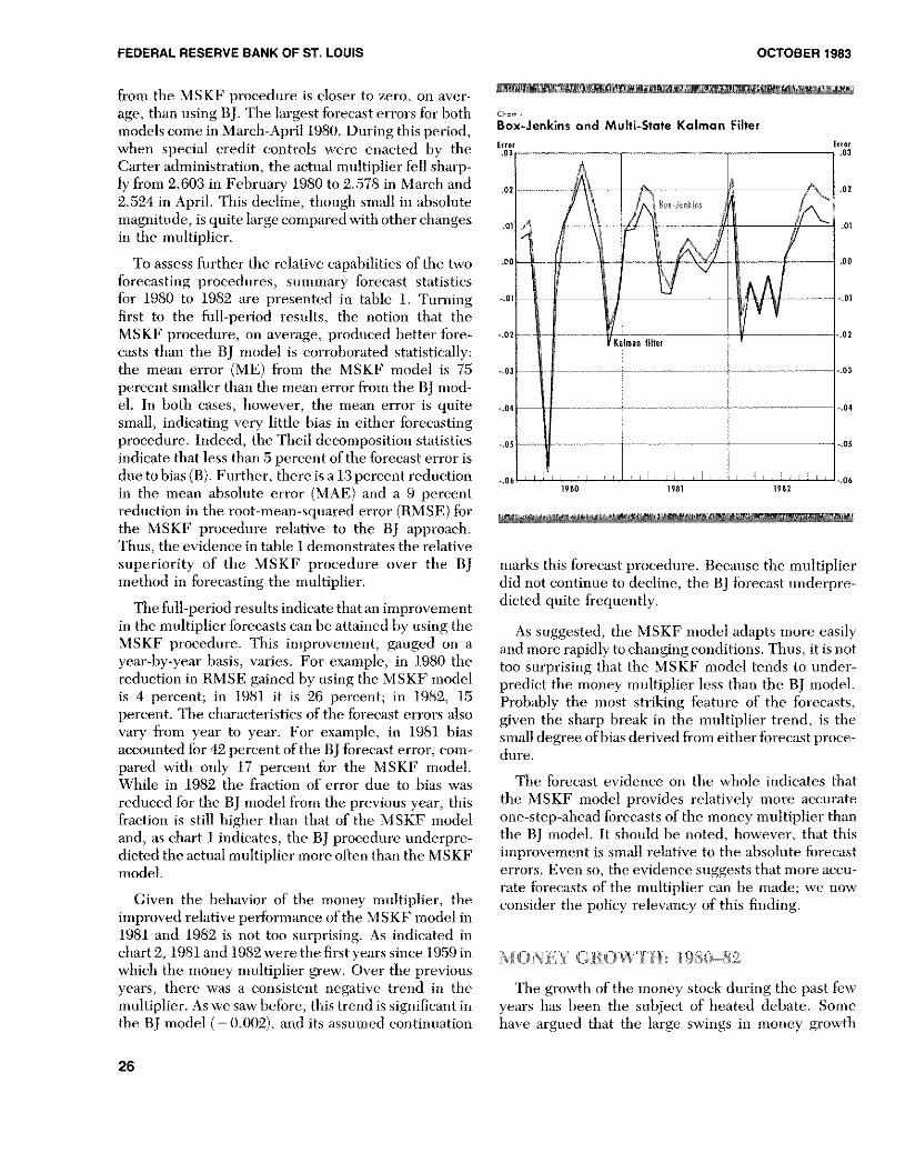
from the MSKF procedure is closer to zero, on aver-age, than using BJ. The largest forecast errors for bothmodels come in March-April 1980. During this period,when special credit controls were enacted by theCarter administration, the actual multiplier fell sharp-ly from 2.603 in February 1980 to 2.578 in March and2.524 in April. This decline, though small in absolutemagnitude, is quite large compared withother changesin the multiplier.

To assess further the relative capabilities of tlae twoforecasting procedures, summary forecast statisticsfor 1980 to 1982 are presented in table 1. Turningfirst to the full-period results, the notion that theMSKF procedure, on average, produced better fore-casts than the BJ model is corroborated statistically;the mean error (ME) from the MSKF model is 75percent smaller than the mean error from the BJ mod-el. In both cases, however, the mean error is quitesmall, indicating very little bias ira either forecastingprocedure. Indeed, the Theil decomposition statisticsindicate that less than 5 percent of the forecast error isdue tobias (B). Further, there is a 13 percent reductionin the mean absolute error (MAE) and a 9 percentreduction in the root-mean-squared error (RMSE) forthe MSKF procedure relative to the BJ approach.Thus, the evidence in table 1 demonstrates the relativesuperiority of the MSKF procedure over the BJmethod in forecasting the multiplier.

The full-period results indicate that an improvementin the multiplier forecasts can be attained by using theMSKF procedure. This improvement, gauged on ayear-by-year basis, varies. For example, in 1980 thereduction in RMSE gained by using the MSKF modelis 4 percent; in 1981 it is 26 percent; in 1982, 15percent. The characteristics of the forecast errors alsovary from year to year. For example, in 1981 biasaccounted for 42 percent of the BJ forecast error, com-pared with only 17 percent for the MSKF model.While in 1982 the fraction of error due to bias wasreduced for the BJ mnodel from the previous year, thisfraction is still higher than that of the MSKF modeland, as chart 1 indicates, the BJ procedure underpre-dicted the actual multiplier more often than the MSKFmodel.

Given the behavior of the money multiplier, theimnproved relative performance of the MSKF model in1981 and 1982 is not too surprising. As indicated inchart 2, 1981 and 1982 were the first years since 1959 inwhich the money multiplier grew. Over the previousyears, there was a consistent negative trend in themultiplier. As we saw before, this trend is significant inthe BJ model (—0.002), and its assumed continuation

c I,a,frs

Box-Jenkins and Multi-State Kalman Filter

marks this forecast procedure. Because the multiplierdid not continue to decline, the BJ forecast underpre-dicted quite frequently.

As suggested, the MSKF model adapts more easilyand more rapidly tochanging conditions. Thus, it isnottoo surprising that the MSKF model tends to under-predict the money multiplier less than tlae BJ model.Probably the most striking feature of the forecasts,given the sharp break in the multiplier trend, is thesmalldegree ofbias derived from either forecast proce-dure.

The forecast evidence on the whole indicates thatthe MSKF model provides relatively more accurateone-step-ahead forecasts of the money multiplier thanthe BJ anode!. It should he noted, however, that thisimprovement is small relative to the absolute forecasterrors. Even so, the evidence suggests that more accu-rate forecasts of the multiplier can be made; we nowconsider the policy relevancy of this finding.

MONEY GROWTH: 1980—S2

The growth of the money stock during the past fewyears has heera the subject of heated debate. Somehave argued tlaat the large swings in money growtla

Error Error.03 .03

1980 1981 1982

26

FEDERAL RESERVE BANK OF ST. LOUIS OCTOBER 1983

Table 1

Summary Statistics for One-Step-Ahead Multiplier Forecasts:January 1980—December 1982

1 1980 -121982 11980— 121980 1 1981 -- 121982 1 1982- 121982Summary .... —

statistics BJ MSKF Bj MSKE BJ MSKF - -- BJ MSKF

ME 00036 00009 0.0009 00023 00068 00035 00048 00015

MAE 00134 00116 00185 00165 00083 00069 00132 0.0115RMSE 0.0168 0.0153 00226 0.0216 00106 00084 00148 0.0129

U 0.0065 00059 0.0088 0.0084 00041 00033 00058 0.0050

B 00459 00035 0.0015 00112 0.4200 01741 01049 00132

V 0 0228 0.0021 0.0061 0.0009 0.0332 0.0954 0 0549 0.0262

C 09314 09944 09924 09879 0.5468 07305 08402 09606

ME isthe mean error; MAE is the mean abso’uteerror. RMSEisthe root-mean squared error. U .sthe med neouaiilycoe~ficient:B, Vanci Crepresent the amount of forecast error due to b’as. variation and covariation. respective

1y. between actual and forecasted series

Level of the Ml Money Multiplier

3.2

1959 60 61 62 63 64 65 66 67 68 69 70 7i 72 73 74 75 76 77 18 79 80 81 i982

27

FEDERAL RESERVE BANKOF ST. LOUIS OCTOBER 1983

resulted from erratic changes in the public’s demandfor money.8 Others have suggested that certain tech-nical changes, such as implementing contempora-neous reserve accounting, revising discount rate policyand the restructuring of reserve requirements, mustbe made in order to better control the money stock.

Table 2 reports the monthly and quarterly growthrates of Ml for the period January 1980 to December1982. The monthly growth rates indicate a significantdegree of variability in the series. During 1980, forexample, the average monthly growth rate for Ml was7.18 percent with a standard deviation of 12.50 per-cent. This relatively high degree of variability is dueprimarily to the large downturn in money growth dur-ing the February-April period when the special creditcontrols were implemented.

The years 1981 and 1982 show a reduction in moneygrowth variability. In 1981, the average monthlygrowth ofMl declined to 6.56 percent with a standarddeviation of 5.97 percent. In 1982, average monthlymoney growth and variability, although smaller than1980, showed some increase over 1981; money growthaveraged 6.56 percent with a standard deviation of6.80percent.

The quarterly growth rates in table 2 also indicate anerratic pattern to money growth. During the threeyears examined, the standard deviations of quarterlyMl growth are 8.60 percent in 1980, 2.85 percent in1981 and 4.71 percent in 1982.

SIMULATING MONEY GROWTH

It has been argued that policymakers could achieve amore stable pattern of quarterly money growth byimplementing the following control procedure;

1) In period t, using all available information, aforecastof the money multiplier for period t + 1 is made.

2) Given this forecast and the level of Ml desired int+ 1, the amount of adjusted monetary base to sup-port that money stock is determined, and the base ischanged toachieve this new desired level. Thus, anydeviation of the money stock from the desired level

5This view is disputed in Scott E- Hem, ‘Short-Run Money Growth

Volatility: Evidence ofMisbehaving Money Demand,” this Review(June/July 1982), pp. 27—36; Kenneth C. Froewiss, ‘Speaking soft-ly But Carrying a Big Stick,” Economic Research (Goldman Sachs,December1982); and John P. Judd, ‘The Recent Decline in Veloc-ity; Instability in Money Demand or Inflation?” Federal ReserveBank ofSan Francisco Economic Review (Spring 1983), pp. 12—19.

3) In period t+ 1, the forecast of the multiplier is re-calculated for t +2, taking into account money multi-plier information available through period t+ 1.

4) Again in t + 1, the adjusted base necessarytoachieve

the desired money stock in t + 2 is calculated.

The process continues month by month, alwaysattempting toachieve the desired level of money stock.Clearly, an accurate money multiplier prediction isimportant for this control procedure to achieve the

is the result solely of a money multiplier forecasterror.

28

FEDERAL RESERVE BANK OF ST. LOUIS OCTOBER 1983

Table 3

Simulating Ml Growth Using Box-Jenkins Multiplier Forecast:January 1 980—December 1982(seasonally adjusted)

Targeted Actual Forecasted Simulated Simuiated SirnulatecMl growth ratePeriod Ml’ multipher multiplier base Ml Monthly Quarterly

11980 $3907 25955 25866 5151.0 $3920 967%21980 3923 26026 2.5909 t514 3941 663 632%31980 3940 25783 25973 1517 3911 87041980 3957 25235 25811 153.3 3869 123551980 397.4 25266 25364 1567 3958 3176 21161980 399.1 25373 25270 157.9 4007 157771980 400.8 25508 25324 1583 4037 93281980 4025 2.5715 25437 1582 4069 995 121591980 4042 2.5812 25620 1578 4072 102

101980 4060 25837 25739 1577 4075 072111980 4077 2.5605 25789 1581 4048 770 065121980 4094 2.5514 25632 1597 4075 852

11981 4161 25612 25523 1630 4176 105021981 4181 25698 25566 1636 4203 8.15 51031981 4202 2.5853 25641 1639 4236 99941981 4222 25964 25775 1638 4253 483

51981 4243 25870 25892 1639 4239 3.87 41961981 4263 25789 25854 1649 4253 39071981 4284 25806 25784 1662 4288 104181981 4305 2.5843 25778 1670 4316 811 6.0991981 4326 2.5834 25804 1676 4331 432101981 4347 2.5807 25804 1685 4348 466111981 4368 25824 25784 1694 4375 781 629121981 4390 25918 25791 1702 4411 10.37

11982 4420 2.6096 25862 1709 4460 158521982 4435 25866 26012 1705 4410 1273 66431982 4449 25826 25882 1719 4440 8424.1982 4464 25689 2.5819 1729 4442 04651982 4479 25661 25701 1743 4472 844 220

61982 449.3 25515 25649 1752 4470 04971982 4508 25542 2.5528 176.6 4511 115181982 4583 25603 25516 1772 4538 762 72091982 4538 25733 25558 177.5 4569 836

10.1982 4552 25881 2.5665 1774 4591 5.93111982 4567 25987 25802 177.0 4600 2.47 558121982 4582 26088 25916 1768 4613 337

‘Billions of dollars

du~u-edminir\ ~Lo&h ohjc( tnt’. In tlii~rnz-tnl. the and. hec anw the pi~tcchIre.ttteiiipts to coiiuet vrrors

\.1SK I’ approat hi ~hiinldeU a qn~uicrI~nioiic\ stock in nione’ ~ro~th ~‘.tcii niontli the inonth—Io—nionth

series ol lower ariahuiiI~ thi.tn liii’ RI model. \U’i ihiiit~ ‘TI (hi simulated growth ratr~lna\ he I LT’4i

An important leature ol tins eoutrol proc cdii re. how —

Rc’fore esanniung the siniiil,ttuiii i’t’sult5. it inn’t he nel , is that it alters the di~trihiutionof nioutbd~Wow LII

noted that the control pi-ocedui-e discussed hvfl is not tales iii sot ii a wa~that growth oLe ariahdit> os el

desigiied to ri’diitt till’ nioiithI~ ~,triahihI’iii \i I qnartei—I~ i’’ loii~ti~time hon/oTis is I~keR to he ic—grow tii Ihe objet ti~e is to achie~i a nionthI~ target duced ( ,fl (TI esisti ig empiric o1 t\ idtnc’t’ Oil the ri H—

29

FEDERAL RESERVE BANK OF ST. LOUIS OCTOBER 1983

tionship between real economic activity and quarterlymoney growth, success can be measured in terms ofthe reduction in the variability of both the quarterlymoney growth series and in economic activity.

Money Growth Simulations: Box-JenkinsMultiplier Forecasts

The money multiplier forecasts generated from theBJ model, reported in table 1, are used to simulatemoney growth from January 1980 to December 1982.°Table 3 summarizes the results using these forecastsand the control procedure described above. The pos-ited Ml growth targets for 1980, 1981 and 1982 are5.25 percent, 6.00 percent and 4.00 percent, respec-tively.

The results in table 3 indicate that, on average, thesimulated level of Ml is close to the desired amount.The largest discrepancies occur in early 1980, theperiod of the special credit controls. For example, thesimulated level of Ml in April 1980 is more than $8billion below the targeted level. As explained, themonthly growth rates for the simulated series are ex-pectedly erratic under this control procedure. Com-pared with the actual Ml growth rate data in table 2,however, the pattern of growth rates is quite different.For example, in 1980, actual Ml increased during thefirst two months at an average rate of 10.7 percent.During the next two months, it declined at an averagerate of 11.7 percent. From April to August, Ml steadilyincreased at an average rate of 15.8 percent and, dur-ing the lastofthe year, increased at a 6.25 percent rate.

~It has been argued that the actual pattern of the multiplier and,therefore, the money stock would have been different had theFederal Reserve operated under a monetary control procedure likethe one discussed in this study. Two points need to he made: First,this argument can be raised against all simulation experiments.Their purpose, after all, is to investigate the outcomes underdifferent sets ofconditions. There is generallyno way to determinethe validity or usefulness of this criticisat.

Second, this argument is based on the assumption that multi-plier forecasts are rendered useless by the endogeneity of themonetary base during the multiplier forecastingperiod. This prob-lem has been examined by Lindsey (and others) and found to affectthe reliability of the type of multiplier Ibrecast procedures em-ployed here. In a recent paper, however, Brunner and Meltzerhave shown that these assertions are highly questionable. Foralternative views, see David Lindsey and others, “Monetary Con-trol Experience Under the New Operating Procedures,” in NewMonetary Control Procedures, Vol. 2, Federal Reserve Staff Study(February 1981); and Karl Brunner and Allan H.Meltzer.Strategies and Tactics for Monetary Control,” in Caniegie-

Rochester Conference Series, Vol. 18 (1983). pp. 59—104.

Table 4Vanablllty *1 Actual and StflntlstedM GrOWS

____ 9—Sumátded uathg nlulstedt

P~k,t Actual BJ MSKF Actual B4 M$KF

isae ta4r itS IES - .1 41

96 $ 41 4 285 ()SD 2619826 4 4 4 84

ability nteaswed by staSard S4abon mgu~wtbS

Simulated Ml based on the BJ multiplier forecastsincreases at a slower 8.2 percent rate in early 1980,then declines at a 10.5 percent rate from Februarythrough April. In May, the simulated Ml figure re-bounds sharply as the procedure attempts to offset theerrors of the previous two months: during the periodApril to August, simulated Ml growth averages 16.7percent. Finally, in contrast to the 6.25 percent rate ofactual Ml growth during the final four months of 1980,simulated Ml averages only a 0.64 percent rate ofgrowth.

The volatility of the simulated jnonthly growth ratescontinues throughout the sample. For comparison, thevariability of the actual and simulated money growthseries are reported in table 4. In each year, thevariability of the simulated growth rate series is aboutthe same as the actual growth rate of money.

Reducing the monthly variability of money growth,however, is not the goal ofthe procedure. One aim is areduction in quarterly growth rate variability. Judgingfrom the evidence in table 3, the approach used heredoes exactly that. ‘°Note that throughout the periodthe swings in quarterly growth rates are reduced. Forinstance, actual Ml growth ranges from 16.94 percentin 111/1980 to —3.84 percent iii IV/1980. The corre-sponding figures for simulated Ml growth are lessvolatile, varying between 12.15 percent in 111/1980and 0.65 percent in IV/1980.

iO~should be noted that the first-quarter growth rates of the simu-

lated series are measured from the actual level of money in theprevious quarter. l’his reflects the common ‘foregiveness princi-ple” ofadjudging money growth from its actual level as opposed tothe desired level.

30

FEDERAL RESERVE BANK OF ST. LOUIS OCTOBER 1983

\\ ~ ~ \~~\4 \‘~\ ~ ~v ,~ ~ ~ , \ /\/~\~ \ ~\~ \\\\ >\// /

\, ~,-, ,, ,~ ~S ~ <‘~,,,/ .y ,~ ~\

Tà~IG5~ ~ / N ~ ~ ~ /v V : ~ ~ / \ \, //

nulat~MtSYSfriS64 Màet V N

JaWuary 4980-fleiem$ti9aftseasonathj *1j~rsle~ V / 7,

~ AØuat ~ ~~tcsastilfl sisujaS swstá V~ ~ Sta hiS’S isSGr’ IDIIØ lta$ V Mt’~ N ~

9*0 ~S9tY 2SV4VVV1003 $3917~~ 043% V

N ~ N\240a ~N&S944 ~ ~V~39M V.O2 /4* /

*4k’ / V / / I /49* ‘~, 4 V V; / / V

/ $b /W VV4S/\ ~96 ~,43a4 /~0T V IOsS~ /

*0*8* $$Y ~ 24~28Ø St44V V/iS? Iti ~8(54 ~/ V

/ V 98*/V ~s / /‘<//V t8*6&~ V ‘tSB~ 460)’,. V

/ / 406)’ / ~ / N ~ / / *11% / 40& ‘V 7/V V

“ Vs$$~ V ~ V” ‘1*8k V /45)’ // 1< / ~ /

/ $4? // /4041/ ~V V *M8t /V~ V / 44t~ t4~” VV / 1

/ ‘40fl~/’ V/~j$~ / 207$’ a // V / /

V tt~ V” 407 ~ ask V 4oL // ~ OS Vt /

// /,‘48$4/V ~‘Z#ø V S c/ eat, / ~1/ / N / V V / // V//

AS N/VVV*S1* ~V ~1$$4C’ V / // 44/V”fJj9~V & ~tSS *4564* / 0/Vt

~ / I$90~’V~ tosó Y4**1~ V/tot/V /V / /

~ 911$t 774221 V/V $34’V// ,4840

V ~/V 7/ 4fl / V V/ V

45/191 ~ C7// V aS$AV 7 / VV~ V V / // / j7 /

428* taOs %$Ws VVIMPV / 4 734/ “ ~N

71*7V *4 3S06~ /~*V / t*IV 743*4 “Vt’tI V

8/S S ,fl$4~ N V~ø4* SI t V /7 iS4334 / \‘~ //~ ~ / / /,~ /

~1*ttOs 4341 ~2~07 1~ 434 434~ NV /7

I 9*1 43* US 2*1* V *2 743flV a ‘~ Sn*198 ~5*e~’ *918/V 24822 t /4 V

V /7 ~VV V ‘V N / V

11*82 4424 46096 2119fl 170 *2352/ V ~ ~‘V/2j4t~ Z600~\ ~V t4?hV \/ 490) ,S9/7 SOON V

s/19T82 /744413 \\ S*20 2S48Ø~\ V 7t~ \V 4444 V /

4/1*82’ 4454 V 25S$OV V 17245 , 44473 ~1G \/ V

$2 44/79 115081/7 ‘245~99 1142/ ~447 C a 2005~982 442$’ *4$5t$\V V 206,64 V 75 4461 1287 982 450$ V15642 V 2$S~ ‘17388/1382 4322 SI, I 40374 621 as91902 4034 2500 772 4521 53 V

10/1982 V as /1714 4500 5)021 1*2 4*7 2488? 2/75*72 V 7~ 45845 98 4aV

I 198 4582 5088 ~2J9& 84’ 4601 364

Bdhot~~*S V V

This reduction in quarterly money growth volatility ‘ -

is made clearer in table 4. There we see that thevolatility of the quarterly money growth derived fromthe BJ multiplier forecasts is appreciably smaller than The outcome from using the MSKF multiplier fore-the actual. In fact, in 1981 and 1982, the volatility of casts to simulate Ml growth is reported in table 5.simulated quarterly Ml growth is less than one-haff Similar to the results using the BJ multiplier forecasts,that of actual Ml growth. Thus, in terms of reducing the simulated Ml growth rates in table 5 exhibit a largequarterly fluctuations in money growth, the control degree of monthly variation. Again, in contrast toprocedure using the BJ multiplier forecasts is quite actual Ml growth, the distribution of monthly growthsuccessful, rates reveals the procedure’s attempt to correct devia-

31

FEDERAL RESERVE BANK OF ST. LOUIS OCTOBER 1983

tions from the desired Ml path. As reported in table 4,the monthly money growth derived from the MSKFforecasts is more variable than either actual moneygrowth or the BJ simulations in 1980 and again in 1982.

This monthly volatility, however, again translatesinto a more stable pattern of quarterly Ml growth.Recall that, during the second half of 1980, simulatedMl growth based on BJ multiplier forecasts variedfrom 0.65 percent to 12.15 percent. Over this period,the MSKF-based figures range from 0.78 percent to10.59 percent. As shown in table 4, quarterly Mlsimulated using the MSKF forecasts is less volatilethan that using the BJ multiplier forecasts in 1980 and1982. This suggests that the MSKF approach providesa steadier path of quarterly money growth than the BJapproach.

The evidence indicates that stable quarterly moneygrowth can be achieved by making use of the multiplierforecasting techniques implemented here. Based onour empirical results, the simulated quarterly moneygrowth series were, on average, about 50 percent lessvariable than actual Ml growth during the past fewyears. Moreover, the simulated series generally camequite close to hitting the desired Ml growth target. Asshowi~in table 6, both simulated money series missedthe annual growth targets by only one percentagepoint, on average.

MONEY GROWTH A~NDECONOMIC

ACTIVITY

Large fluctuations in quarterly Ml growth have ledsome observers to conclude that the pattern of eco-nomic activity during the 1980—82 period is attribut-able largely to volatile monetary policy actions. In-deed, empirical evidence for the United States andother countries suggests a close association betweensubstantial short-run declines in money growth fromits trend and the pace of economic activity. 11 During

11Historical evidence on this point for the United States is pre-

sented in Clark Warburton, “Bank Reserves and Business Fluc-tuations,” Journal of the American Statistical Association (De-cember 1948), pp. 547—58; Milton Friedman and Anna J.Schwartz, “Money and Business Cycles,” Review of Economicsand Statistics (Supplement: February 1963), pp. 32—78; and Wil-liam Poolc, “The Relationship ofMonetary Decelerations to Busi-ness Cycle Peaks: Another Look at the Evidence,” Journal ofFinance (June 1975), pp. 697—712. An analysis ofmore recent datafor the United States along with several other countries can befound in Dallas S. Batten and R. W. Hafer, “Short-Run Mouey

Table 6

Comparison of Desired and SimulatedMl Growth Rates

Simulated Ml

Desired Ml

Period growth MSKF BJ

IV’1979”1V.’1980 525% 4.82% 4.96%

IV’1980--IVl98i 6.00 7.69 7.67

IV’1981-IV.1982 400 4.96 5.10

our SLTII~I&,such dc\ jations occurrcd in Carl)’ i9.SU andagain in 1981. In this regard, reducing money growthfluctuations, everything else equal, should producemore stable economic growth. To examine this hypoth-esis, the following experiment was conducted: First, astandard, St. Louis type of reduced-form equation fornominal CNP growth was estimated over the period111960 to IV/1979. Then, using the estimated coef-ficients, CNP growth was simulated for the period111980 to IV/1982. Three simulation runs were made:one with actual Ml growth, one with the posited pathof Ml and one based on Ml growth from the MSKFmoney growth simulations. (The BJ simulations areomitted because they were so similar to the MSKF.)

The simulated GNP growth rates for each experi-ment are reported in table 7. 12 The volatility of actualMl growth is evident in the consequent fluctuations ofGNP growth, especially in 1980 when GNP growthfluctuated from 6.81 percent to 12.69 percent. For thewhole period, nominal GNP growth simulated withactual money growth averages 10.46 percent with astandard deviation of 1.94 percent.

The pattern of GNP growth simulated under theposited Ml path of 5.25 percent growth in 1980, 6.0

Growth Fluctuations and Real Economic Activity: Some Implica-tions for MonetaryTargeting,” this Review (May1982), pp. 15—20.

12The equation used to generate the simulations is (t-statisties inparentheses):

4 4= 2.507 + 1.052 X + 0.068 X

(2.14) (5.34) i=0 (0.68) i”O

= 0.33 SE = 3.52 DW = 1.95where 1’ is nominal GNP growth, 1%~Jis the growth of Ml and ft isthe growth of high-employment government expenditures. Theequation is estimated for the period I/1960=IV/1979 using afourth-order Almon polynomial lag for each of the explanatoryvariables with endpoints constrained, All simulations use actualE.

32

FEDERAL RESERVE BANKOF ST. LOUIS OCTOBER 1983

Table 7

Simulated Quarterly GNP GrowthRates: I/i 980—IV/i 982

Simuuated values

derived from

Period Actual Ml Desired Ml MSKF

11980 ll06°~ 1050% 10.37°II 681 898 824III 981 904 990IV 1269 923 926

11981 1270 924 841II 1212 889 7.13III 10.41 9.96 841

IV 905 1023 979

11982 915 837 898II 847 723 769III 1018 816 916IV 1304 857 9.80

Mean 10.46 903 893Standarddeviation 1 94 0 92 0 98

percent growth in 1981 and 4.0 percent growth in 1982is very different from that simulated with actual Mlgrowth. For one thing, the average GNP growth simu-lated with actual money is almost 1.5 percentage pointsabove that simulated with the desired path. It is only in11/1980 and IV/l98l that GNP growth based on actualmoney is less than CNP growth based on desiredmoney. In addition to the difference in mean growthrates, there is also a sizeable difference in the volatilityof CNP growth under the alternative simulations. Asmeasured by the standard deviation of GNP growth,the simulations with actual money show more thantwice the volatility than the simulations with desiredmoney yield.

Comparisons between simulations using actual anddesired money growth presumes that the desiredmoney growth easily can be achieved. As we haveseen, however, the Fed cannot totally control moneygrowth from one quarter to the next. How serious aproblem is this? Would this lack of precise controlmake it difficult to achieve a less volatile GNP growthobjective?

To examine this issue, the GNP equation was simu-lated using the Ml growth rates that resulted from theMSKF money multiplier forecasting control proce-dure. These simulated CNP growth rates are shown inthe third column of table 7. There is surprisingly littledifference between the CNP growth simulated usingdesired Ml growth and Ml growth resulting from theforecast/control procedure. The average level of GNPgrowth under the desired Ml growth scenario is 9.03percent, compared with9.08 percent under the MSKFprocedure. The standard deviation of simulated GNPgrowth is less than one percent in both cases — aboutone-half that associated with actual Ml growth. Inaddition, the simulated CNP path using the quarterlygrowth of money derived from the MSKF forecastprocedure usually is within one percentage point ofthesimulated GNP path using desired Ml growth.

SUMMARY AND CONCLUSION

This paper has examined two alternative proceduresto forecast the Ml multiplier. The multiplier was fore-cast one period ahead for the 1980—82 sample periodusing both a Box-Jenkins and a Multi-State KalmanFilter forecast procedure. The evidence from the mul-tiplier forecasts shows the MSKF procedure to be animprovement over the BJ procedure. For example, theMSKF yielded a root-mean-squared error about 9 per-cent smaller than the BJ procedure for the wholeperiod, with even greater reduction in forecast error in1981 and 1982.

Both forecasts of the multiplier then were used tosimulate Ml growth. These simulations resulted involatile monthly growth rates, but relatively stablequarterly growth rates. There was, in fact, little differ-ence between the simulated Ml growth rates, suggest-ing that forecasting the multiplier with great accuracymay not be as important as aiming for a steady long-rungrowth rate.

The paper also examined the importance of moneystock control by simulating GNP growth under thehypothetical desired path, as well as the Ml growthsimulated under the MSKF forecast/control proce-dure. There was only a minor difference in these simu-lations; quarterly CNP growth usually did not differ bymore than one percentage point. This indicates thatthe money multiplier forecast/control procedure usedin this article could be successful in achieving morestable GNP growth.

33