Forecasting the Equity Risk Premium:The Role of Technical Indicators

Christopher J. NeelyFederal Reserve Bank of

St. Louisneely@stls.frb.org

David E. RapachSaint Louis University

rapachde@slu.edu

Jun TuSingapore Management

Universitytujun@smu.edu.sg

Guofu Zhou∗Washington University in

St. Louis and CAFRzhou@wustl.edu

January 8, 2012

∗Corresponding author. Send correspondence to Guofu Zhou, Olin School of Business, Washington University in St. Louis, St. Louis,MO 63130; e-mail: zhou@wustl.edu; phone: 314-935-6384. This project began while Rapach and Zhou were Visiting Scholars at theFederal Reserve Bank of St. Louis. We thank seminar participants at the Cheung Kong Graduate School of Business, 2011 China Inter-national Conference in Finance, Federal Reserve Bank of St. Louis, Forecasting Financial Markets 2010 Conference, Fudan University,Saint Louis University, Singapore Management University 2010 Summer Finance Camp, Temple University, Third Annual Confer-ence of The Society for Financial Econometrics, University of New South Wales, 2010 Midwest Econometrics Group Meetings, HankBessembinder, William Brock, Henry Cao, Long Chen, Todd Clark, John Cochrane, Robert Engle, Miguel Ferreira, Mark Grinblatt,Bruce Grundy, Massimo Guidolin, Harrison Hong, Jennifer Huang, Raymond Kan (2011 CICF discussant), Michael McCracken, AdrianPagan, Jesper Rangvid, Pedro Santa-Clara, Jack Strauss, and George Tauchen for helpful comments. The usual disclaimer applies. Tuacknowledges support from SMU Internal Research Grant C207/MSS10B001. The views expressed in this paper are those of the authorsand do not reflect those of the Federal Reserve Bank of St. Louis or the Federal Reserve System.

Forecasting the Equity Risk Premium:The Role of Technical Indicators

Abstract

Do existing equity risk premium forecasts ignore useful information, such as technical indicators? Al-though academics have extensively used macroeconomic variables to forecast the U.S. equity risk premium,they have paid relatively little attention to the technical stock market indicators widely employed by practi-tioners. Our paper fills this gap by studying the forecasting ability of technical indicators relative to popularmacroeconomic variables. We find that technical indicators display statistically and economically significantout-of-sample forecasting power and generate substantial utility gains; moreover, technical indicators tendto detect the typical decline in the equity risk premium near cyclical peaks, while macroeconomic variablesmore readily pick up the typical rise near cyclical troughs. In line with this cyclical behavior, utilizing in-formation from both technical indicators and macroeconomic variables substantially increases out-of-sampleforecasting performance relative to either alone.

JEL classification: C53, C58, E32, G11, G12, G17

Key words: equity risk premium predictability; macroeconomic variables; moving-average rules; momen-tum; Volume; out-of-sample forecasts; asset allocation; business cycle

1. IntroductionA voluminous literature studies U.S. equity risk premium prediction with macroeconomic variables. Rozeff

(1984), Fama and French (1988), and Campbell and Shiller (1988a, 1988b) present evidence that valuation ra-

tios, such as the dividend yield, predict the U.S. equity risk premium. Similarly, Keim and Stambaugh (1986),

Campbell (1987), Breen, Glosten, and Jagannathan (1989), and Fama and French (1989) find predictive ability

for nominal interest rates and the default and term spreads, while Nelson (1976) and Fama and Schwert (1977)

detect predictive capability for the inflation rate. Recent studies confirm equity risk premium predictability using

valuation ratios (Cochrane 2008, Pastor and Stambaugh 2009), interest rates (Ang and Bekaert 2007), and infla-

tion (Campbell and Vuolteenaho 2004). Additional macroeconomic variables, such as the consumption-wealth

ratio (Lettau and Ludvigson 2001) and volatility (Guo 2006), also exhibit predictive power. Ang and Bekaert

(2007), Hjalmarsson (2010), and Henkel, Martin, and Nadari (2011) find equity risk premium predictability

based on macroeconomic variables across countries. Cochrane (2011) explains how this predictability literature

profoundly shifts the emphasis of asset pricing theory from expected cash flows to discount rates.

The degree of return predictability is small, however. The influential study of Goyal and Welch (2008)

argues that out-of-sample criteria are important for assessing stock return predictability. In light of this, recent

studies rely on the Campbell and Thompson (2008) out-of-sample R2 statistic (R2OS), which measures the reduc-

tion in mean squared forecast error (MSFE) for a competing forecast relative to the historical average (constant

expected excess return) benchmark forecast, as well as utility gains for investors. In terms of these metrics, Fer-

reira and Santa-Clara (2011) provide the best-to-date forecast of the U.S. equity risk premium with their intrigu-

ing “sum-of-the-parts” approach, which more efficiently exploits macro information. For the 1966:01–2008:12

evaluation period, the sum-of-the-parts forecast generates a monthly R2OS of 1.18% and annualized utility gain of

2.97% for a mean-variance investor with a risk aversion coefficient of five. By focusing on macroeconomic vari-

ables, however, recent studies ignore a specific type of information that practitioners commonly use: technical

indicators.

Technical indicators, such as moving averages and price-momentum signals, represent market price reac-

tions and other market statistics. Such indicators potentially capture information relevant for forecasting stock

market returns beyond that summarized by macroeconomic variables. Indeed, technical indicators are read-

ily available from newspapers and newsletters and are an important component of the information set used by

traders and investors (e.g., Billingsley and Chance 1996, Covel 2005, Park and Irwin 2007, Lo and Hasanhodzic

2010). Despite the widespread use of technical indicators, relatively few academic papers study their predictive

ability. Although early studies (e.g., Cowles 1933, Fama and Blume 1966, Jensen and Benington 1970) typi-

cally find little ability for technical indicators to track future stock returns, more recent studies provide much

stronger evidence that technical indicators work. For example, Brock, Lakonishok, and LeBaron (1992) present

evidence that moving averages based on the Dow Jones Industrial Average generate profitable trading signals,

while Lo, Mamaysky, and Wang (2000) find that technical analysis implemented via kernel estimators and au-

tomated rules provides incremental information that adds value to the investment process.1 Existing studies

of technical analysis focus on the profitability of trading signals, which essentially predict the sign of market

1Relative to equity markets, academic studies generally find stronger support for the efficacy of technical analysis in foreign exchangemarkets. For example, LeBaron (1999) and Neely (2002) show that moving averages generate substantial portfolio gains for currencytrading and that the gains are much larger than those in the stock market. Moreover, Menkhoff and Taylor (2007) argue that technicalanalysis today is as important as fundamental analysis to currency mangers.

1

returns, and do not forecast the magnitude of the equity risk premium with technical indicators.

Our paper is the first to compare and combine the power of macroeconomic variables and technical indicators

for forecasting the equity risk premium. We begin by analyzing equity risk premium forecasts based on technical

indicators with the R2OS statistic. We transform the technical indicators into equity risk premium forecasts using

a recursive predictive regression framework. This allows us to directly compare equity risk premium forecasts

based on technical indicators with those based on macroeconomic variables in terms of MSFE. We analyze the

forecasting ability of a variety of technical indicators, including popular moving-average (MA), momentum,

and volume-based technical indicators.

Following Campbell and Thompson (2008), among others, we also analyze the economic value of equity

risk premium forecasts based on technical indicators and macroeconomic variables from an asset allocation

perspective. Specifically, we calculate utility gains for a mean-variance investor who optimally allocates a

portfolio between equities and risk-free Treasury bills using equity risk premium forecasts based on either

technical indicators or macroeconomic variables relative to an investor who uses the historical average equity

risk premium forecast. While a number of studies investigate the profitability of technical indicators, these

studies are ad hoc in that they do not account for risk aversion in the asset allocation decision. Analogous to

Zhu and Zhou (2009), we address this drawback and compare the utility gains for a risk-averse investor who

forecasts the equity risk premium using technical indicators to those for an identical investor who forecasts the

equity risk premium with macroeconomic variables.

Our results indicate that monthly equity risk premium forecasts based on technical indicators produce eco-

nomically significant R2OS statistics and utility gains and frequently outperform forecasts based on popular

macroeconomic variables. Furthermore, the out-of-sample forecasting gains are highly concentrated in NBER-

dated business-cycle recessions for both technical indicators and macroeconomic variables. This is especially

evident for the utility metric. For example, a mean-variance investor with a risk aversion coefficient of five would

pay an annualized portfolio management fee of 3.58% to have access to the equity risk premium forecast based

on a monthly MA(2,12) technical indicator relative to the historical average benchmark forecast for the entire

1966:01–2008:12 forecast evaluation period; during recessions, the same investor would pay a hefty annualized

fee of 19.51%. Insofar as predictability is linked to the real economy, we expect that there will be more pre-

dictability in the rapidly changing economic conditions of recessions (e.g., Henkel, Martin, and Nadari 2011).

The relatively high predictability during recessions is consistent with the stock price continuation/trend story of

Zhang (2006), who incorporates behavioral insights from Daniel, Hirshleifer, and Subrahmanyam (1998, 2001)

and Hirshleifer (2001). When volatility is high, as in recessions relative to expansions, information uncertainty

is also high. In this environment, investors are more likely to underreact to information, which produces stock

price trends and greater return predictability based on technical indicators.

Although technical indicators and macroeconomic variables both forecast better than the historical average

benchmark during recessions, the two approaches exploit different patterns: technical indicators detect the

typical fall in the equity risk premium near cyclical peaks, while macroeconomic variables tend to pick up

the typical rise in the equity risk premium later in recessions near cyclical troughs. This suggests that technical

indicators and macroeconomic variables provide complementary information over the business cycle. To further

investigate this complementarity, we combine information from both technical indicators and macroeconomic

variables. In particular, we compute an equity risk premium forecast from a predictive regression with a small

2

number of principal components extracted from the complete set of technical indicators and macroeconomic

variables. This approach guards against in-sample overfitting when estimating the forecasting model in the

presence of a large number of potential predictors.2 Combining information from both technical indicators and

macroeconomic variables appears very useful. Relative to the Ferreira and Santa-Clara (2011) sum-of-the-parts

approach, the R2OS increases by about 40%, from 1.18% to 1.66%, while the annualized utility gain increases

by nearly 80%, from 2.97% to 5.32%, over the 1966:01–2008:12 evaluation period. These results help to

explain the simultaneously prominent roles for the macroeconomic variables used in the academic literature

and technical indicators used by practitioners: both approaches seem useful for predicting returns, and they

complement each other.

Overall, our findings suggest that technical indicators are at least as useful as macroeconomic variables

and capture additional relevant information for forecasting the equity risk premium. Existing theoretical asset

pricing models typically ignore the information investors have about technical indicators, and our study calls

for new asset pricing models that can improve our understanding of the role of technical indicators and their

equilibrium pricing impacts.3

2. Econometric Methodology2.1. Forecast Construction

The conventional framework for analyzing equity risk premium predictability based on macroeconomic

variables is the following predictive regression model:

rt+1 = αi +βixi,t + εi,t+1, (1)

where rt+1 is the return on a broad stock market index in excess of the risk-free rate from period t to t +1, xi,t

is a predictor (e.g., the dividend yield), and εi,t+1 is a zero-mean disturbance term. Following Campbell and

Thompson (2008) and Goyal and Welch (2003, 2008), we generate an out-of-sample forecast of rt+1 based on

(1) and information through t as

ri,t+1 = αi,t + βi,txi,t , (2)

where αi,t and βi,t are the ordinary least squares (OLS) estimates of αi and βi, respectively, in (1) computed by

regressing {rk}tk=2 on a constant and {xi,k}t−1

k=1. Dividing the total sample of T observations into q1 in-sample

and q2 out-of-sample observations, where T = q1 + q2, we can calculate a series of out-of-sample equity risk

premium forecasts based on xi,t over the last q2 observations: {ri,t+1}T−1t=q1 .4 The historical average of the equity

2This is similar to Ludvigson and Ng (2007, 2009), who use principal component forecasts to extract information from a very largenumber of macroeconomic variables to predict stock and bond returns.

3Behavioral models offer potential explanations for the predictive ability of technical indicators, especially during recessions, al-though these models have not typically been formalized for technical indicators per se. As previously discussed, Zhang (2006) finds thatstock-price underreaction is magnified when there is greater information uncertainty. Furthermore, Hong and Stein (1999) and Hong,Lim, and Stein (2000) provide both theory and empirical evidence on the slow transmission of bad news in financial markets. Recessionsare presumably associated with large adverse macroeconomic news shocks, which may take longer to be fully incorporated into stockprices. As a result, the market will exhibit stronger trending patterns during recessions, creating greater scope for trend-based technicalindicators to forecast equity prices. Consistent with this is the disposition effect—investors tend to hold losers too long and sell winnerstoo early (Odean 1998). During the early stages of recessions, there are more share price declines and hence more losers; this impliesthat the disposition effect is stronger in recessions, thereby reinforcing the stronger trend.

4Observe that the forecasts are generated using a recursive (i.e., expanding) window for estimating αi and βi in (1). Forecasts couldalso be generated using a rolling window (which drops earlier observations as additional observations become available) in recognition

3

risk premium, rt+1 = (1/t)∑tk=1 rk, is a natural benchmark forecast corresponding to the constant expected

excess return model (βi = 0 in (1)). Goyal and Welch (2003, 2008) show that rt+1 is a stringent benchmark:

predictive regression forecasts based on macroeconomic variables frequently fail to outperform the historical

average forecast in out-of-sample tests.

Campbell and Thompson (2008) demonstrate that parameter and forecast sign restrictions improve individ-

ual forecasts based on macroeconomic variables, allowing them to more consistently outperform the historical

average equity risk premium forecast. For example, theory often indicates the expected sign of βi in (1), so

that we set βi = 0 when forming a forecast if the estimated slope coefficient does not have the expected sign.

Campbell and Thompson (2008) also suggest setting the equity risk premium forecast to zero if the predictive

regression forecast is negative, since risk considerations typically imply a positive expected equity risk premium

based on macroeconomic variables. We impose Campbell and Thompson (2008) restrictions on the individual

predictive regression forecasts.

We consider three popular types of technical indicators. The first is an MA rule that, in its simplest form,

generates a buy or sell signal (St = 1 or St = 0, respectively) at the end of t by comparing two moving averages:

St =

{1 if MAs,t ≥MAl,t

0 if MAs,t < MAl,t, (3)

where

MA j,t = (1/ j)j−1

∑i=0

Pt−i for j = s, l, (4)

Pt is the level of a stock price index, and s (l) is the length of the short (long) MA (s < l). We denote the MA

rule with MA lengths s and l as MA(s, l). Intuitively, the MA rule is designed to detect changes in stock price

trends. For example, when prices have recently been falling, the short MA will tend to be lower than the long

MA. If prices begin trending upward, then the short MA tends to increase faster than the long MA, eventually

exceeding the long MA and generating a buy signal. In Section 3, we analyze monthly MA rules with s = 1,2,3

and l = 9,12.

The second type of technical indicator we consider is based on momentum. A simple momentum rule

generates the following signal:

St =

{1 if Pt ≥ Pt−m

0 if Pt < Pt−m. (5)

Intuitively, a current stock price that is higher than its level m periods ago indicates “positive” momentum

and relatively high expected excess returns, which generates a buy signal. We denote the momentum rule that

compares Pt to Pt−m as MOM(m), and we compute monthly signals for m = 9,12 in Section 3.

Technical analysts frequently employ volume data in conjunction with past prices to identify market trends.

In light of this, the final type of technical indicator we consider incorporates “on-balance” volume (e.g., Granville

1963). We first define

OBVt =t

∑k=1

VOLkDk, (6)

of potential structural instability. Pesaran and Timmermann (2007) and Clark and McCracken (2009), however, show that the optimalestimation window for a quadratic loss function can include pre-break data due to the familiar bias-efficiency tradeoff. We use recursiveestimation windows in Section 3, although we obtain similar results using rolling estimation windows of various sizes.

4

where VOLk is a measure of the trading volume during k and Dk is a binary variable that takes a value of 1 if

Pk−Pk−1 ≥ 0 and −1 otherwise. We then form a trading signal from OBVt as

St =

{1 if MAOBV

s,t ≥MAOBVl,t

0 if MAOBVs,t < MAOBV

l,t

, (7)

where

MAOBVj,t = (1/ j)

j−1

∑i=0

OBVt−i for j = s, l. (8)

Intuitively, relatively high recent volume together with recent price increases, say, indicate a strong positive

market trend and generate a buy signal. In Section 3, we compute monthly signals for s = 1,2,3 and l = 9,12

and denote the corresponding rule as VOL(s,l).

The MA, momentum, and volume-based indicators conveniently capture the trend-following idea at the

center of technical analysis and are representative of the technical indicators analyzed in the academic literature

(e.g., Sullivan, Timmermann, and White 1999). To directly compare these technical indicators to equity risk

premium forecasts based on macroeconomic variables, we transform the technical indicators to point forecasts

of the equity risk premium by replacing the macroeconomic variable xi,t in the predictive regression, (1), with

St from (3), (5), or (7). We then generate out-of-sample equity risk premium forecasts using St as the explana-

tory variable in a manner analogous to the forecasts based on macroeconomic variables described earlier. To

further facilitate comparison with predictive regression forecasts based on macroeconomic variables, we set the

predictive regression forecast based on a technical indicator to zero if the unrestricted forecast is negative.

2.2. Forecast EvaluationWe consider two metrics for evaluating forecasts based on macroeconomic variables and technical indica-

tors. The first is the Campbell and Thompson (2008) R2OS statistic, which measures the proportional reduction

in MSFE for a competing model relative to the historical average benchmark:

R2OS = 1− ∑

q2k=1(rq1+k− rq1+k)

2

∑q2k=1(rq1+k− rq1+k)2 , (9)

where rq1+k represents an equity risk premium forecast based on a macroeconomic variable or technical indi-

cator. Clearly, when R2OS > 0, the competing forecast outperforms the historical average benchmark in terms of

MSFE. We employ the Clark and West (2007) MSFE-adjusted statistic to test the null hypothesis that the com-

peting model MSFE is greater than or equal to the historical average MSFE against the one-sided alternative

hypothesis that the competing forecast has a lower MSFE, corresponding to H0 : R2OS ≤ 0 against HA : R2

OS > 0.5

R2OS statistics are typically small for equity risk premium forecasts, but even a relatively small R2

OS statistic

can signal economically important gains for an investor (Kandel and Stambaugh 1996, Xu 2004, Campbell and

Thompson 2008). From an asset allocation perspective, however, the utility gain itself is the key metric. As a

second metric for evaluating forecasts, we thus compute realized utility gains for a mean-variance investor who

optimally allocates across stocks and risk-free bills, as in, among others, Marquering and Verbeek (2004) and

5Clark and West (2007) develop the MSFE-adjusted statistic by modifying the familiar Diebold and Mariano (1995) and West(1996) statistic so that it has an approximately standard normal asymptotic distribution when comparing forecasts from nested models.Comparing the forecasts based on technical indicators or macroeconomic variables with the historical average forecast entails comparingnested models, since setting βi = 0 in (1) yields the constant expected excess return model.

5

Campbell and Thompson (2008). As discussed in the introduction, this procedure addresses the weakness of

many existing studies of technical indicators that fail to incorporate the degree of risk aversion into the asset

allocation decision.

In particular, we compute the average utility for a mean-variance investor with risk aversion coefficient of

five who monthly allocates between stocks and risk-free bills using an equity risk premium forecast based on

a macroeconomic variable or technical indicator. Following Campbell and Thompson (2008), we assume that

the investor uses a five-year moving window of past monthly returns to estimate the variance of the equity risk

premium, and we constrain the equity weight in the portfolio to lie between 0% and 150%. We then calculate

the average utility for the same investor using the historical average forecast of the equity risk premium. The

utility gain is the difference between the two average utilities. We multiply this difference by 1200, so that it

can be interpreted as the annual percentage portfolio management fee that an investor would be willing to pay

to have access to the equity risk premium forecast based on a technical indicator or macroeconomic variable

relative to the historical average forecast.

3. Empirical ResultsThis section describes the data and reports out-of-sample test results for the R2

OS statistics and average utility

gains.

3.1. DataOur monthly data span 1927:01–2008:12. The data are from Amit Goyal’s web page, which provides

updated data from Goyal and Welch (2008).6 The aggregate market return is the continuously compounded

return on the S&P 500 (including dividends), and the equity risk premium is the difference between the aggregate

market return and the log return on a risk-free bill. The following 14 macroeconomic variables, which are well

representative of the literature (Goyal and Welch 2008), constitute the set of macroeconomic variables used to

forecast the equity risk premium:

1. Dividend-price ratio (log), DP: log of a twelve-month moving sum of dividends paid on the S&P 500

index minus the log of stock prices (S&P 500 index).

2. Dividend yield (log), DY: log of a twelve-month moving sum of dividends minus the log of lagged stock

prices.

3. Earnings-price ratio (log), EP: log of a twelve-month moving sum of earnings on the S&P 500 index

minus the log of stock prices.

4. Dividend-payout ratio (log), DE: log of a twelve-month moving sum of dividends minus the log of a

twelve-month moving sum of earnings.

5. Stock variance, SVAR: monthly sum of squared daily returns on the S&P 500 index.

6. Book-to-market ratio, BM: book-to-market value ratio for the Dow Jones Industrial Average.

7. Net equity expansion, NTIS: ratio of a twelve-month moving sum of net equity issues by NYSE-listed

stocks to the total end-of-year market capitalization of NYSE stocks.

8. Treasury bill rate, TBL: interest rate on a three-month Treasury bill (secondary market).

9. Long-term yield, LTY: long-term government bond yield.

10. Long-term return, LTR: return on long-term government bonds.

6The data are available at http://www.hec.unil.ch/agoyal/.

6

11. Term spread, TMS: long-term yield minus the Treasury bill rate.

12. Default yield spread, DFY: difference between BAA- and AAA-rated corporate bond yields.

13. Default return spread, DFR: long-term corporate bond return minus the long-term government bond

return.

14. Inflation, INFL: calculated from the CPI (all urban consumers); we follow Goyal and Welch (2008) and

use xi,t−1 in (1) for inflation to account for the delay in CPI releases.

We use the S&P 500 index for Pt when computing the technical indicators based on the MA and momentum

rules in (3) and (5), respectively. In addition to the S&P 500 index, we use monthly volume data (beginning in

1950:01) from Google Finance to compute the trading signal in (7).7

3.2. R2OS Statistics

Panel A of Table 1 reports R2OS statistics (in percent) for monthly predictive regression forecasts based

on macroeconomic variables over the 1966:01–2008:12 forecast evaluation period. We use 1927:01–1965:12

as the initial in-sample period when forming the recursive out-of-sample forecasts. We assess the statistical

significance of R2OS using the Clark and West (2007) MSFE-adjusted statistic, as described in Section 2.2. R2

OS

statistics are computed separately for the full 1966:01–2008:12 forecast evaluation period, as well as NBER-

dated expansions and recessions.8 The U.S. economy is in recession for 77 of the 516 months (15%) spanning

1966:01–2008:12.

According to the second column of Table 1, Panel A, nine of the 14 individual macroeconomic variables

produce positive R2OS statistics over the full 1966:01–2008:12 out-of-sample period, so that they outperform

the historical average benchmark forecast in terms of MSFE. Three of the nine positive R2OS statistics for the

individual macroeconomic variables are significant at the 10% level or better. DP and DY have the highest R2OS

statistics, 0.54% and 0.77%, respectively, among the individual macroeconomic variables. The fourth and sixth

columns of Table 1 report R2OS statistics separately for business-cycle expansions and recessions, respectively.

Recessions markedly enhance the out-of-sample predictive ability of most macroeconomic variables compared

to the historical average. For example, the predictive ability of DP and DY is highly concentrated in recessions:

the R2OS statistics for DP (DY) are −0.10% and 2.06% (−0.20% and 3.06%) during expansions and recessions,

respectively. The R2OS statistics for DP, DY, LTR, and TMS are significant at the 10% level during recessions,

despite the reduced number of available observations; the R2OS for NTIS (0.01%) is the only statistic that is

significant during expansions for the macroeconomic variables.

To illustrate how equity risk premium forecasts vary over the business cycle, Figure 1 graphs predictive

regression forecasts based on individual macroeconomic variables, along with the historical average benchmark.

The vertical bars in the figure depict NBER-dated recessions. Many of the individual predictive regression

forecasts—especially those that perform the best during recessions, such as DP, DY, and TMS—often increase

substantially above the historical average forecast over the course of recessions, reaching distinct local maxima

near cyclical troughs. This is particularly evident during more severe recessions, such as the mid 1970s and

7The volume data are available at http://www.google.com/finance. While daily data are frequently used to generate technical indica-tors, we compute technical indicators using monthly data to put the forecasts based on macroeconomic variables and technical indicatorson a more equal footing. In ongoing research, we are investigating the use of daily data to generate monthly trading signals to study themore practical problem of maximizing portfolio performance using technical indicators.

8NBER peak and trough dates that define the expansion and recession phases of the U.S. business cycle are available athttp://www.nber.org/cycles.html.

7

early 1980s. The countercyclical fluctuations in equity risk premium forecasts in Figure 1 are similar to the

countercyclical fluctuations in in-sample expected equity risk premium estimates reported in, for example, Fama

and French (1989), Ferson and Harvey (1991), Whitelaw (1994), Harvey (2001), and Lettau and Ludvigson

(2009). The fifth and seventh columns of Table 1, Panel A show that the average equity risk premium forecast

is higher during recessions than expansions for a number of macroeconomic variables, including DP and DY.

Figure 2 provides a time-series perspective on the out-of-sample predictive ability of macroeconomic vari-

ables over the business cycle. The figure portrays the cumulative differences in squared forecast errors between

the historical average forecast and forecasts based on individual macroeconomic variables.9 A segment of the

curve that is higher (lower) at its end point relative to its initial point indicates that the competing forecast out-

performs (underperforms) the historical average forecast in terms of MSFE over the period corresponding to the

segment. The curves are predominantly positively sloped—sometimes quite steeply—during many recessions

in Figure 2 (with the notable exception of NTIS); outside of recessions, the curves are often flat or negatively

sloped. Overall, Figure 2 provides further evidence of the enhanced predictive power of macroeconomic vari-

ables during recessions.

We turn next to the forecasting performance of the technical indicators in Table 1, Panel B. For the MA

and momentum indicators in (3) and (5), respectively, we use 1927:12–1965:12 or 1928:01–1965:12 as the

initial in-sample period to estimate the predictive regression model that transforms the trading signals to point

forecasts.10 Data availability limits the starting date for the volume rules’ in-sample period to 1950:12.11 The

second column of Table 1, Panel B shows that twelve of the 14 individual technical forecasts have positive R2OS

statistics for 1966:01–2008:12, so that they outperform the historical average forecast according to the MSFE

metric. Eight of the twelve positive R2OS statistics are significant at conventional levels. Comparing the results in

Panels A and B of Table 1, equity risk premium forecasts based on technical indicators generally provide more

sizable out-of-sample gains than forecasts based on macroeconomic variables.

The fourth and sixth columns of Table 1, Panel B show even starker differences in forecasting performance

across business-cycle phases for the forecasts based on technical indicators in Panel B compared to the forecasts

based on macroeconomic variables in Panel A. Eleven of the 14 individual technical forecasts exhibit negative

R2OS statistics during expansions, while all forecasts have positive R2

OS statistics during recessions; twelve of the

positive statistics during recessions are significant at conventional levels. Moreover, the R2OS statistics for the

technical forecasts are quite sizable during recessions, with many ranging from around 1.5% to close to 4%.

Figure 3 shows that the technical forecasts almost always drop below the historical average forecast—often

substantially so—throughout recessions. There are also expansionary episodes where some of the technical

forecasts frequently fall below the historical average forecast. The fourth column of Table 1, Panel B indicates

that these declines detract from the accuracy of these technical forecasts during expansions. The fifth and

seventh columns of Panel B show that the average technical forecasts of the equity risk premium are uniformly

lower during recessions than expansions.

Analogous to Figure 2, Figure 4 graphs the cumulative differences in squared forecast errors between the

9Goyal and Welch (2003, 2008) employ this device to assess the consistency of out-of-sample predictive ability.10These starting dates allow for the lags necessary to compute the initial MA or momentum signal in (3) or (5).11This starting date for the volume rules’ in-sample period motivates our selection of 1966:01 as the start of the forecast evaluation

period, since this provides us with approximately 15 years of data for estimating the predictive regression parameters used to computethe initial forecast based on a volume rule.

8

historical average forecast and technical forecasts. The positive slopes of the curves during recessions in Figure

4 show that most of the technical forecasts consistently produce out-of-sample gains during these periods. But

the curves are almost always flat or negatively sloped for expansions, so that out-of-sample gains are nearly

limited to recessions. Taken together, the results in Table 1 and Figures 2 and 4 highlight the relevance of

business-cycle fluctuations for out-of-sample equity risk premium predictability using either macroeconomic

variables or technical indicators.

3.3. Utility GainsTable 2 reports average utility gains, in annualized percent, for a mean-variance investor with risk aversion

coefficient of five who allocates monthly across stocks and risk-free bills using equity risk premium forecasts

derived from macroeconomic variables (Panel A) or technical indicators (Panel B).12 The results in Panel A

indicate that forecasts based on macroeconomic variables often produce sizable utility gains vis-a-vis the his-

torical average benchmark. The utility gain is above 1% for seven of the individual macroeconomic variables

in the second column, so that the investor would be willing to pay an annual management fee of more than

100 basis points to have access to forecasts based on macroeconomic variables relative to the historical average

forecast. Similar to Table 1, the out-of-sample gains are concentrated in recessions. Consider, for example, DY,

which generates the largest utility gain (2.47%) for the full 1966:01–2008:12 forecast evaluation period. The

utility gain is negative (−0.21%) during expansions, while it is a very sizable 17.17% during recessions. DP,

TBL, LTY, and TMS also provide utility gains above 8% during recessions.

Figure 5 portrays the equity portfolio weights computed using equity risk premium forecasts based on

macroeconomic variables and historical average forecasts. Because the investor uses the same volatility forecast

for all of the portfolio allocations, only the equity risk premium forecasts produce differences in the equity

weights. Figure 5 shows that the equity weight computed using the historical average forecast (gray line) is

procyclical, which, given that the historical average forecast of the equity risk premium is relatively smooth,

primarily reflects countercyclical changes in expected volatility.13 The equity weights based on macroeconomic

variables (black lines) often deviate substantially from the equity weight based on the historical average, with

a tendency for the weights computed using macroeconomic variables to lie below the historical average weight

during expansions and move closer to or above the historical average weight during recessions. Panel A of Table

2 indicates that these deviations create significant utility gains for our mean-variance investor, especially during

recessions.

The second column of Table 2, Panel B shows that all 14 of the utility gains for forecasts based on technical

indicators are positive for the full 1966:01–2008:12 out-of-sample period. Twelve of the individual technical

forecasts provide utility gains above 1.5%, with the MA(2,12) forecast generating the largest gain (3.58%).

Comparing the fourth and sixth columns, the utility gains are substantially higher and more consistent during

recessions than during expansions. The MA(1,9) forecast provides a leading example: the utility gain is negative

during expansions (−0.51%), while it jumps to 16.95% during recessions. In all, ten of the individual technical

forecasts produce utility gains above 12% during recessions. The fifth and seventh columns reveal that the

12For the asset allocation exercises, we measure the equity risk premium and compute forecasts in terms of simple (instead of log)returns, so that the portfolio return is given by the sum of the individual portfolio weights multiplied by the asset returns.

13French, Schwert, and Stambaugh (1987), Schwert (1989, 1990), Whitelaw (1994), Harvey (2001), Ludvigson and Ng (2007),Lundblad (2007), and Lettau and Ludvigson (2009), among others, also find evidence of countercyclical expected volatility usingalternative volatility estimators.

9

average equity weight is substantially lower during recessions than expansions for all of the technical forecasts.

Figure 6 further illustrates that technical forecast weights (black lines) tend to decrease during recessions,

dropping below the weight based on the historical average forecast during cyclical downturns. Again recalling

that the investor uses the same rolling-window variance estimator for all portfolio allocations, these declining

weights reflect decreases in the technical forecasts during recessions, as discussed in the context of Figure 3.

Overall, Table 2 shows that equity risk premium forecasts based on both macroeconomic variables and

technical indicators usually generate sizable utility gains, especially during recessions, highlighting the eco-

nomic significance of equity risk premium predictability using either approach. Comparing Panels A and B

of Table 2, forecasts based on technical indicators typically provide larger utility gains than forecasts based on

macroeconomic variables over the full 1966:01–2008:12 forecast evaluation period and during recessions.

3.4. A Closer Look at Forecast Behavior Near Cyclical Peaks and TroughsTables 1 and 2 and Figures 1–6 present somewhat of a puzzle. Out-of-sample gains are typically concen-

trated in recessions for equity risk premium forecasts based on both macroeconomic variables and technical

indicators. However, equity risk premium forecasts based on macroeconomic variables often increase during

recessions, while forecasts based on technical indicators are usually substantially lower during recessions than

expansions. Despite the apparent differences in the behavior of the two types of forecasts during recessions, the

out-of-sample gains are concentrated in cyclical downturns for both approaches. Why?

We investigate this issue by examining the behavior of the actual equity risk premium and forecasts around

cyclical peaks and troughs, which define the beginnings and ends of recessions, respectively. We first estimate

the following regression model around cyclical peaks:

rt − rt = aP +4

∑k=−2

bP,kIPk,t + eP,t , (10)

where IPk,t is an indicator variable that takes a value of unity k months after an NBER-dated peak and zero

otherwise. The estimated bP,k coefficients measure the incremental change in the average difference between

the realized equity risk premium and historical average forecast k months after a cyclical peak. We then estimate

a corresponding model that replaces the actual equity risk premium, rt , with an equity risk premium forecast

based on a macroeconomic variable or technical indicator:

rt − rt = aP +4

∑k=−2

bP,kIPk,t + eP,t . (11)

The slope coefficients describe the incremental change in the average difference between a forecast based on a

macroeconomic variable or technical indicator relative to the historical average forecast k periods after a cyclical

peak. Similarly, we measure the incremental change in the average behavior of the realized equity risk premium

and the forecasts around cyclical troughs:

rt − r = aT +∑2k=−4 bT,kIT

k,t + eT,t , (12)

rt − rt = aT +∑2k=−4 bT,kIT

k,t + eT,t , (13)

where ITk,t is an indicator variable equal to unity k months after an NBER-dated trough and zero otherwise.

10

The top-left panel of Figure 7 graphs OLS slope coefficient estimates (in percent) and 90% confidence bands

for (10), and the remaining panels depict corresponding estimates for (11) based on individual macroeconomic

variables. The top-left panel shows that the actual equity risk premium tends to move significantly below the

historical average forecast one month before through two months after a cyclical peak. The remaining panels in

Figure 7 indicate that most macroeconomic variables fail to pick up this decline in the equity risk premium early

in recessions. Only the LTR, TMS, and INFL forecasts are significantly below the historical average forecast

for any of the months early in recessions when the equity risk premium itself is lower than average, although

the size of the decline in the INFL forecast is very small. The TMS forecast does the best job of matching the

lower-than-average actual equity risk premium for the month before through two months after a peak. However,

the TMS forecast is also significantly lower than the historical average forecast two months before and three

and four months after a peak, unlike the actual equity risk premium. Overall, Figure 7 suggests that equity risk

premium forecasts based on macroeconomic variables fail to detect the decline in the equity risk premium near

cyclical peaks.

How do the equity risk premium forecasts based on technical indicators behave near cyclical peaks? The

top-left panel of Figure 8 again shows estimates for (10), while the other panels graph estimates for (11) based

on individual technical indicators. Figure 8 reveals that most of the technical forecasts move substantially below

the historical average forecast in the months immediately following a cyclical peak, in accord with the behavior

of the actual equity risk premium. Given that the actual equity risk premium moves substantially below average

in the month before and month of a cyclical peak, it is not surprising that technical forecasts are nearly all lower

than the historical average in the first two months after a peak, since the technical forecasts are based on signals

that recognize trends in equity prices. This trend-following behavior early in recessions apparently helps to

generate the sizable out-of-sample gains during recessions for the technical forecasts in Tables 1 and 2. The

forecasts based on technical indicators in Figure 8 tend to remain well below the historical average for too long

after a peak, however.

Figures 9 and 10 depict estimates of the slope coefficients in (12) and (13) for forecasts based on macroe-

conomic variables and technical indicators, respectively. The top-left panel in each figure shows that the actual

equity risk premium moves significantly above the historical average forecast in the third and second months

before a cyclical trough, so that the equity risk premium is higher than usual in the late stages of recessions.

Figure 9 indicates that many of the forecasts based on macroeconomic variables, particularly those based on

DP, DY, EP, BM, and LTR, are also significantly higher than the historical average forecast in the third and

second months before a trough. The TMS forecast is also well above the historical average in the later stages

of recessions, although by less than the previously mentioned macroeconomic variables. The ability of many of

the forecasts based on macroeconomic variables to match the higher-than-average equity risk premium late in

recessions helps to account for the sizable out-of-sample gains during recessions for forecasts based on macroe-

conomic variables in Tables 1 and 2.

Figure 10 shows that forecasts based on technical indicators typically start low but rise quickly late in

recessions, in contrast to the pattern in the actual equity risk premium. The out-of-sample gains for the technical

forecasts during recessions in Tables 1 and 2 thus occur despite the relatively poor performance of technical

forecasts late in recessions. While the trend-following technical forecasts detect the decrease in the actual

equity risk premium early in recessions (see Figure 8), they do not recognize the unusually high actual equity

11

risk premium late in recessions.

In summary, Figures 7–10 paint the following nuanced picture with respect to the sizable out-of-sample

gains during recessions in Tables 1 and 2. Macroeconomic variables typically fail to detect the decline in the

actual equity risk premium early in recessions, but generally do detect the increase in the actual equity risk

premium late in recessions. Technical indicators exhibit the opposite pattern: they pick up the decline in the

actual premium early in recessions, but fail to match the unusually high premium late in recessions. Although

both types of forecasts generate substantial out-of-sample gains during recessions, they capture different aspects

of equity risk premium fluctuations during cyclical downturns. This suggests that fundamental and technical

analysis provide complementary approaches to out-of-sample equity risk premium predictability. We explore

this complementarity further in the next section.

4. Technical Indicators and Macro Variables in ConjunctionHeretofore, we have generated equity risk premium forecasts using individual macroeconomic variables and

technical indicators. Can employing macroeconomic variables and technical indicators in conjunction produce

additional out-of-sample gains?

Including all of the potential regressors simultaneously or using in-sample model selection methods can

overfit the data, leading to poor out-of-sample forecasts. To tractably incorporate information from all of the

macroeconomic variables and technical indicators, while avoiding in-sample over-fitting, we use a principal

component approach. Let xt = (x1,t , . . . ,xN,t)′ denote the N-vector of potential predictors; N = 28 in our appli-

cation, since we have 14 macroeconomic variables and 14 technical indicators. Let fk,t = ( f1,k,t , . . . , fJ,k,t)′ for

k = 1, . . . , t represent the vector comprised of the first J principal components of xt estimated using data avail-

able through t, where J� N. Intuitively, the principal components conveniently detect the key comovements in

xt , while filtering out much of the noise in individual predictors. We then use a predictive regression framework

to generate a principal component (PC) forecast of rt+1:

rPC,t+1 = αPC,t + β′PC,t ft,t , (14)

where αPC,t and βPC,t are the OLS intercept and J-vector of slope coefficient estimates, respectively, from

regressing {rk}tk=2 on a constant and { fk,t}t−1

k=1. Ludvigson and Ng (2007, 2009) use a PC approach to predict

stock and bond market returns based on a very large number of macroeconomic variables, while we use such an

approach to incorporate information from a large number of macroeconomic variables and technical indicators to

forecast the equity risk premium. For consistency, we continue to impose the non-negativity forecast restriction.

An important issue in constructing the PC forecast is the selection of J, the number of principal components

to include in (14). We need J to be relatively small to avoid an overly parameterized model; at the same time, we

do not want to include too few principal components, thereby neglecting important information in xt . We select

J using the Onatski (2011) ED algorithm. This algorithm displays good properties for selecting the true number

of factors in approximate factor models for sample sizes near ours in simulations in Onatski (2011). The ED

algorithm typically selects J = 3 when forming recursive PC forecasts using the 14 macroeconomic variables

and 14 technical indicators.

Panel A of Table 3 reports R2OS statistics for the PC forecast for the full 1966:01–2008:12 forecast evaluation

period and separately during expansions and recessions. The R2OS statistic is 1.66% for the full period, which

12

is significant at the 1% level and well above all of the corresponding R2OS statistics for the forecasts based on

individual macroeconomic variables and technical indicators in Table 1. Similar to the results in Table 1, the

PC forecast R2OS is substantially higher during recessions (4.37%, significant at the 1% level) than expansions

(0.50%, significant at the 10% level). The R2OS statistics for the PC forecast during expansions and recessions

are higher than each of the corresponding R2OS statistics in Table 1.14

The top panel of Figure 11 depicts the time series of PC equity risk premium forecasts. The PC forecast

exhibits a close connection to the business cycle. In particular, the PC forecast is typically well below the

historical average forecast near cyclical peaks. At the same time, the PC forecast moves well above the historical

average forecast near cyclical troughs corresponding to more severe recessions. This cyclical pattern in the PC

forecast indicates that it incorporates the relevant information from both macroeconomic variables and technical

indicators that enhances equity risk premium predictability, as discussed in Section 3.

Analogous to Figures 2 and 4, the middle panel of Figure 11 graphs the difference in cumulative squared

forecast errors for the historical average forecast relative to the PC forecast. The curve is predominantly posi-

tively sloped throughout the 1966:01–2008:12 period, so that the PC forecast delivers out-of-sample gains on a

consistent basis over time, much more consistently than any of the forecasts based on individual macroeconomic

variables or technical indicators in Figures 2 and 4. The curve is frequently steeply sloped during recessions,

again highlighting the importance of business-cycle fluctuations for equity risk premium predictability.

The PC forecast also generates substantial utility gains from an asset allocation perspective, as evidenced

by Table 3, Panel B. The utility gain is 5.32% for the full 1966:01–2008:12 forecast evaluation period, which

is well above any of the corresponding utility gains for forecasts based on individual macroeconomic variables

and technical indicators in Table 2. Continuing the familiar pattern, the utility gains are concentrated during

economic contractions, with gains of 1.39% and 27.25% during expansions and recessions, respectively. The

gains during expansions and recessions are again greater than any of the corresponding gains in Table 2. The

average equity weights reported in the last row of Table 2 show that the average equity weight is lower during

recessions vis-a-vis expansions (0.10 and 0.39, respectively). Inspection of the bottom panel of Figure 11 shows

that the average equity weight of 0.10 during recession masks sizable shifts in asset allocation during recessions:

the PC forecast typically leads the investor to move entirely out of stocks near cyclical peaks and throughout

much of the downturn; however, the investor tends to move aggressively back into stocks late in recessions near

cyclical troughs of severe recessions. In contrast, the historical forecast is much less capable of “timing” the

market near cyclical peaks and troughs.

“Data snooping” concerns naturally arise when considering a host of potential predictors. To control for

data snooping, we use a modified version of White’s (2000) reality check due to Clark and McCracken (2012).

The Clark and McCracken (2012) reality check is based on a wild fixed-regressor bootstrap and is appropri-

ate for comparing forecasts from multiple models that all nest the benchmark model, as in our framework.15

14We also generated a PC forecast based on the first prinicpal component of the 14 macroeconomic variables, so that informationfrom the technical indicators is excluded. The PC forecast based on macroeconomic variables alone has an R2

OS of 0.96% for thefull 1966:01–2008:12 forecast evaluation period (significant at the 1% level). This is less than the R2

OS of 1.66% for the PC forecastthat includes information from both the macroeconomic variables and technical indicators, so that incorporating information from thetechnical indicators improves the PC forecast. Furthermore, the Clark and West MSFE-adjusted statistic indicates that the MSFE for thePC forecast based on the 14 macroeconomic variables and 14 technical indicators taken together is significantly less than the MSFE forthe PC forecast based only on the 14 macroeconomic variables at the 5% level.

15As Clark and McCracken (2012) emphasize, the asymptotic and finite-sample properties of the non-parametric bootstrap procedurein White’s (2000) reality check, as well as Hansen’s (2005) modified reality check, do not generally apply when comparing forecasts

13

Specifically, we test the null hypothesis that the MSFE for each of the competing models is greater than or

equal to the MSFE for the historical average benchmark against the alternative hypothesis that at least one of the

competing models has a lower MSFE. This corresponds to a test of H0: R2OS,m ≤ 0 for all m = 1, . . . ,M, where

m indexes a competing model, against HA: R2OS,m > 0 for at least one m. We implement this test using the Clark

and McCracken (2012) maxMSFE-Fm statistic:

maxMSFE-Fm = maxm=1,...,M

q2dm

MSFEm, (15)

where q2 is the size of the forecast evaluation period,

dm = (1/q2)q2

∑k=1

[(rk− rk)

2− (rk− rm,k)2] , (16)

MSFEm = (1/q2)q2

∑k=1

(rk− rm,k)2. (17)

In our application, M = 29, corresponding to the 14 forecasts based on individual macroeconomic variables, 14

forecasts based on individual technical indicators, and the PC forecast. For the 1966:01–2008:12 forecast eval-

uation period, the maxMSFE-Fm statistic equals 8.70, with a wild fixed-regressor bootstrap p-value of 4.7%, so

that we reject the null hypothesis that none of the competing models outperforms the historical average bench-

mark in terms of MSFE at conventional significance levels.16 This reality check indicates that data snooping

cannot readily explain the out-of-sample equity risk premium predictability in Tables 1 and 3.

Finally, we compare the out-of-sample gains from the PC forecast, which incorporates information from

both macroeconomic variables and technical indicators, to two recently proposed methods for improving out-

of-sample equity risk premium forecasts. Rapach, Strauss, and Zhou (2010) show that a combination forecast

delivers consistent out-of-sample gains relative to equity risk premium forecasts based on individual macroeco-

nomic variables. Using the same approach, we form a combination forecast as the mean of the forecasts based

on the 14 individual macroeconomic variables that we consider. This combination forecast produces an R2OS of

0.63% and utility gain of 1.62% for the 1966:01–2008:12 forecast evaluation period.17 These values are both

well below the R2OS of 1.66% and utility gain of 5.32% for the PC forecast in Table 3 during this period.

Ferreira and Santa-Clara (2011) develop an intriguing “sum-of-the-parts” (SOP) approach to forecast the

market return. Specifically, they decompose the log market return into the sum of the growth in the price-

earnings ratio, growth in earnings, and the dividend-price ratio. Treating earnings growth as largely unfore-

castable and the dividend-price and earnings-price ratios as approximately random walks, Ferreira and Santa-

Clara (2011) propose the SOP equity risk premium forecast as the sum of a 20-year moving average of earnings

growth rates and the current dividend-price ratio (minus the risk-free rate).18 They show that the SOP fore-

from multiple models that all nest the benchmark model. Clark and McCracken (2012) show that a wild fixed-regressor bootstrapprocedure for maximum statistics delivers asymptotically valid critical values. They also find that this bootstrap procedure has goodfinite-sample properties.

16The wild fixed-regressor bootstrap used to compute the p-value is described in detail in the appendix.17Rapach, Strauss, and Zhou (2010) report an R2

OS of 3.58% and utility gain of 2.34% for quarterly (instead of monthly) equity riskpremium forecasts for the 1965:1–2005:4 forecast evaluation period.

18Ferreira and Santa-Clara (2011) focus on forecasting the market return, but note that they obtain similar results for the equity riskpremium.

14

cast outperforms equity risk premium forecasts based on individual macroeconomic variables over the postwar

period, primarily by reducing estimation error. For the 1966:01–2008:12 forecast evaluation period, the SOP

forecast generates an R2OS of 1.18% and utility gain of 2.97%.19 These values are larger than the corresponding

values for any of the individual macroeconomic variables in Tables 1 and 2, as well as those for the combination

forecast. However, the R2OS and utility gain for the SOP forecast are substantially lower than the corresponding

values of 1.66% and 5.32% for the PC forecast in Table 3. In short, the ability of the PC forecast to outper-

form the combination and SOP forecasts further establishes the relevance of technical indicators for equity risk

premium forecasting.

5. ConclusionWe analyze monthly out-of-sample forecasts of the U.S. equity risk premium based on popular technical in-

dicators in comparison to a set of well-known macroeconomic variables. We find that technical indicators have

statistically and economically significant out-of-sample forecasting power and frequently outperform macroe-

conomic variables. While both approaches perform disproportionately well during recessions, they exploit very

different patterns: technical indicators recognize the typical drop in the equity risk premium near cyclical peaks;

macroeconomic variables identify the typical increase in the equity risk premium near cyclical troughs. Building

on this complementarity, we generate a principal component equity risk premium forecast, which incorporates

information from all of the technical indicators and macroeconomic variables taken together. The principal

component forecast delivers substantially larger out-of-sample gains than any of the forecasts based on indi-

vidual technical indicators or macroeconomic variables. These gains show that both technical indicators and

macroeconomic variables are important for forecasting the U.S. equity risk premium.

Appendix: Wild Fixed-Regressor BootstrapThis appendix outlines the wild fixed-regressor bootstrap used to calculate the p-value for the maxMSFE-

Fm statistic given by (15). We first estimate the constant expected equity risk premium model, corresponding

to the null of no predictability: r = (1/T )∑Tt=1 rt . We next estimate an unrestricted model that includes all of

the potential predictors as regressors using OLS; denote the OLS residuals from this model as {ut}Tt=1. We then

generate a pseudo sample of equity risk premium observations under the null of no predictability as rbt = r+vb

t ut

for t = 1, . . . ,T , where vbt is a draw from an i.i.d. N(0,1) process. Generating pseudo disturbance terms in this

manner allows for conditional heteroskedasticity and makes this a “wild” bootstrap. Denote the pseudo sample

of equity risk premium observations as {rbt }T

t=1. We compute forecasts based on individual macroeconomic

variables and technical indicators, as well as the PC forecast, for the last q2 simulated equity risk premium

observations using {rbt }T

t=1 in conjunction with the macroeconomic variables and technical indicators from the

original sample. Using macroeconomic variables and technical indicators from the original sample makes this

a “fixed-regressor” bootstrap. Based on {rbt }T

t=q1+1 and the simulated forecasts, we compute the maxMSFE-Fm

statistic for the pseudo sample, maxMSFE-Fbm. Generating B = 10,000 pseudo samples in this manner yields

an empirical distribution of maxMSFE-Fm statistics, {maxMSFE-Fbm}B

b=1. The boostrapped p-value is given

by B−1∑

Bb=1 Ib, where Ib = 1 for maxMSFE-Fb

m ≥ maxMSFE-Fm and zero otherwise and maxMSFE-Fm is the

relevant statistic computed from the original sample.

19The R2OS of 1.18% is reasonably near the R2

OS of 1.32% (0.98%) for the market return reported by Ferreira and Santa-Clara (2011)for the 1948:01–2007:12 (1977:01–2007:12) forecast evaluation period.

15

ReferencesAng, A., G. Bekaert. 2007. Return predictability: Is it there? Review of Financial Studies 20 651–707.

Billingsley, R. S., D. M. Chance. 1996. The benefits and limits of diversification among commodity trading

advisors. Journal of Portfolio Management 23 65–80.

Breen, W., L. R. Glosten, R. Jagannathan. 1989. Economic significance of predictable variations in stock index

returns. Journal of Finance 64 1177–1189.

Brock, W., J. Lakonishok, B. LeBaron. 1992. Simple technical trading rules and the stochastic properties of

stock returns. Journal of Finance 47 1731–1764.

Campbell, J. Y. 1987. Stock returns and the term structure. Journal of Financial Economics 18 373–399.

Campbell, J. Y., R. J. Shiller. 1988a. The dividend-price ratio and expectations of future dividends and discount

factors. Review of Financial Studies 1 195–228.

Campbell, J. Y., R. J. Shiller. 1988b. Stock prices, earnings, and expected dividends. Journal of Finance 43661–676.

Campbell, J. Y., S. B. Thompson. 2008. Predicting the equity premium out of sample: Can anything beat the

historical average? Review of Financial Studies 21 1509–1531.

Campbell, J. Y., T. Vuolteenaho. 2004. Inflation illusion and stock prices. American Economic Review 94 19–23.

Clark, T. E., M. W. McCracken. 2009. Improving forecast accuracy by combining recursive and rolling fore-

casts. International Economic Review 50 363–395.

Clark, T. E., M. W. McCracken. 2012. Reality checks and nested forecast model comparisons. Journal of Busi-

ness and Economic Statistics, forthcoming.

Clark, T. E., K. D. West. 2007. Approximately normal tests for equal predictive accuracy in nested models. Jour-

nal of Econometrics 138 291–311.

Cochrane, J. H. 2008. The dog that did not bark: A defense of return predictability. Review of Financial Studies

21 1533–1575.

Cochrane, J. H. 2011. Discount rates. Journal of Finance 66 1047–1108.

Covel, M. W. 2005. Trend Following: How Great Traders Make Millions in Up or Down Markets. Prentice-Hall,

New York.

Cowles, A. 1933. Can stock market forecasters forecast? Econometrica 1 309–324.

Daniel, K., D. Hirshleifer, A. Subrahmanyam. 1998. Investor psychology and security market over- and under-

reactions. Journal of Finance 53 1839–1886.

Daniel, K., D. Hirshleifer, A. Subrahmanyam. 2001. Overconfidence, arbitrage, and equilibrium asset pric-

ing. Journal of Finance 56 921–965.

Diebold, F. X., R. S. Mariano. 1995. Comparing predictive accuracy. Journal of Business and Economic Statis-

tics 13 253–263.

Fama, E. F., M. F. Blume. 1966. Filter rules and stock market trading. Journal of Business 39 226–241.

Fama, E. F., K. R. French. 1988. Dividend yields and expected stock returns. Journal of Financial Economics

22 3–25.

Fama, E. F., K. R. French. 1989. Business conditions and expected returns on stocks and bonds. Journal of

Financial Economics 25 23–49.

Fama, E. F., G. W. Schwert. 1977. Asset returns and inflation. Journal of Financial Economics 5 115–146.

16

Ferreira, M. A., P. Santa-Clara. 2011. Forecasting stock market returns: The sum of the parts is more than the

whole. Journal of Financial Economics 100 514–537.

Ferson, W. E., C. R. Harvey. 1991. The variation of equity risk premiums. Journal of Political Economy 99385–415.

French, K. R., G. W. Schwert, R. F. Stambaugh. 1987. Expected stock returns and volatility. Journal of Financial

Economics 19 3–29.

Goyal, A., I. Welch. 2003. Predicting the equity premium with dividend ratios. Management Science 49 639–

654.

Goyal, A., I. Welch. 2008. A comprehensive look at the empirical performance of equity premium predic-

tion. Review of Financial Studies 21 1455–1508.

Granville, J. 1963. Granville’s New Key to Stock Market Profits. Prentice-Hall, New York.

Guo, H. 2006. On the out-of-sample predictability of stock market returns. Journal of Business 79 645–670.

Hansen, P. R. 2005. A test for superior predictive ability. Journal of Business and Economic Statistics 23 365–

380.

Harvey, C. R. 2001. The specification of conditional expectations. Journal of Empirical Finance 8 573–637.

Henkel, S. J., J. S. Martin, F. Nadari. 2011. Time-varying short-horizon predictability. Journal of Financial

Economics 99 560–580.

Hirshleifer, D. 2001. Investor psychology and asset pricing. Journal of Finance 56 1533–1596.

Hjalmarsson, E. 2010. Predicting global stock returns. Journal of Financial and Quantitative Analysis 45 49–80.

Hong, H., J. C. Stein. 1999. A unified theory of underreaction, momentum trading and overreaction in asset

markets. Journal of Finance 54 2143–2184.

Hong, H., T. Lim, T., J. C. Stein. 2000. Bad news travels slowly: Size, analyst coverage, and the profitability of

momentum strategies. Journal of Finance 55 265–295.

Jensen, M. C., G. A. Benington. 1970. Random walks and technical theories: Some additional evidence. Journal

of Finance 25 469–482.

Kandel, S., R. F. Stambaugh. 1996. On the predictability of stock returns: An asset allocation perspective.

Journal of Finance 51 385–424.

Keim, D. B., R. F. Stambaugh. 1986. Predicting returns in the stock and bond markets. Journal of Financial

Economics 17 357–390.

LeBaron, B. 1999. Technical trading rule profitability and foreign exchange intervention. Journal of Interna-

tional Economics 49 125–143.

Lettau, M., S. Ludvigson. 2001. Consumption, aggregate wealth, and expected stock returns. Journal of Finance

56 815–849.

Lettau, M., S. C. Ludvigson. 2009. Measuring and modeling variation in the risk-return tradeoff. In Y. Aıt-

Sahalıa, L. P. Hansen (Eds.), Handbook of Financial Econometrics. Elsevier, Amsterdam.

Lo, A. W., J. Hasanhodzic. 2010. The Evolution of Technical Analysis: Financial Prediction from Babylonian

Tablets to Bloomberg Terminals. John Wiley & Sons, Hoboken, New Jersey.

Lo, A. W., H. Mamaysky, J. Wang. 2000. Foundations of technical analysis: Computational algorithms, statisti-

cal inference, and empirical implementation. Journal of Finance 55 1705–1765.

17

Ludvigson, S. C., S. Ng. 2007. The empirical risk-return relation: A factor analysis approach. Journal of Finan-

cial Econometrics 83 171–222.

Ludvigson, S. C., S. Ng. 2009. Macro factors in bond risk premia. Review of Financial Studies 22 5027–5067.

Lundblad, C. 2007. The risk return tradeoff in the long run: 1836–2003. Journal of Financial Economics 85123–150.

Marquering, W., M. Verbeek. 2004. The economic value of predicting stock index returns and volatility. Journal

of Financial and Quantitative Analysis 39 407–429.

Menkhoff, L., M. P. Taylor. 2007. The obstinate passion of foreign exchange professionals: Technical analy-

sis. Journal of Economic Literature 45 936–972.

Neely, C. J. 2002. The temporal pattern of trading rule returns and exchange rate intervention: Intervention does

not generate technical trading profits. Journal of International Economics 58 211–232.

Nelson, C. R. 1976. Inflation and the rates of return on common stock. Journal of Finance 31 471–483.

Odean, T. 1998. Are investors reluctant to realize their losses? Journal of Finance 53 1775–1798.

Onatski, A. 2011. Determining the number of factors from empirical distributions of eigenvalues. Review of

Economics and Statistics, forthcoming.

Park, C.-H., S. H. Irwin. 2007. What do we know about the profitability of technical analysis? Journal of

Economic Surveys 21 786–826.

Pastor, L., R. F. Stambaugh. 2009. Predictive systems: Living with imperfect predictors. Journal of Finance 641583–1628.

Pesaran, M. H., A. Timmermann. 2007. Selection of estimation window in the presence of breaks. Journal of

Econometrics 137 134–161.

Rapach, D. E., J. K. Strauss, G. Zhou. 2010. Out-of-sample equity premium prediction: Combination forecasts

and links to the real economy. Review of Financial Studies 23 821–862.

Rozeff, M. S. 1984. Dividend yields are equity risk premiums. Journal of Portfolio Management 11 68–75.

Schwert, G. W. 1989. Why does stock market volatility change over time? Journal of Finance 44 1115–1153.

Schwert, G. W. 1990. Stock volatility and the crash of ’87. Review of Financial Studies 3 77–102.

Sullivan, R., A. Timmermann, H. White. 1999. Data-snooping, technical trading rule performance, and the

bootstrap. Journal of Finance 54 1647–1691.

West, K. D. 1996. Asymptotic inference about predictive ability. Econometrica 64 1067–1084.

White, H. 2000. A reality check for data snooping. Econometrica 68 1097–1126.

Whitelaw, R. F. 1994. Time variations and covariations in the expectation and volatility of stock market re-

turns. Journal of Finance 49 515–541.

Xu, Y. 2004. Small levels of predictability and large economic gains. Journal of Empirical Finance 11 247–275.

Zhang, X. F. 2006. Information uncertainty and stock returns. Journal of Finance 61 105–136.

Zhu, Y., G. Zhou. 2009. Technical analysis: An asset allocation perspective on the use of moving averages. Jour-

nal of Financial Economics 92 519–544.

18

Table 1 Out-of-Sample Equity Risk Premium Forecasting Results, 1966:01–2008:12

Overall Expansion Recession

Predictor R2OS (%) Average forecast (%) R2

OS (%) Average forecast (%) R2OS (%) Average forecast (%)

Panel A: Forecasts Based on Individual Macroeconomic Variables

DP 0.54∗∗ 0.21 −0.10 0.18 2.06∗∗ 0.41DY 0.77∗∗ 0.18 −0.20 0.14 3.06∗∗∗ 0.39EP −0.37 0.40 −0.42 0.35 −0.27 0.71DE −1.63 0.76 −1.42 0.77 −2.13 0.72SVAR −0.07 0.51 −0.09 0.51 −0.01 0.48BM −0.99 0.41 −1.06 0.33 −0.83 0.85NTIS −1.58 0.77 0.01∗ 0.74 −5.29 0.91TBL 0.13 0.26 −0.19 0.27 0.85 0.18LTY 0.35∗ 0.22 −0.03 0.23 1.23 0.16LTR 0.24 0.56 −0.72 0.55 2.49∗∗∗ 0.61TMS 0.02 0.63 −0.54 0.65 1.31∗ 0.48DFY 0.001 0.50 −0.03 0.49 0.08 0.52DFR 0.21 0.50 0.03 0.51 0.64 0.46INFL 0.12 0.46 0.12 0.48 0.13 0.35

Panel B: Forecasts Based on Individual Technical Indicators

MA(1,9) 0.31 0.51 −1.18 0.57 3.79∗∗∗ 0.15MA(1,12) 1.14∗∗ 0.54 0.19 0.62 3.36∗∗∗ 0.11MA(2,9) 0.71∗∗ 0.51 −0.53 0.58 3.59∗∗∗ 0.13MA(2,12) 1.23∗∗∗ 0.55 0.26 0.62 3.49∗∗∗ 0.11MA(3,9) 0.63∗∗ 0.50 −0.07 0.56 2.28∗∗ 0.17MA(3,12) 0.50∗ 0.50 0.02 0.56 1.63∗ 0.15MOM(9) 0.52∗ 0.58 −0.22 0.66 2.24∗∗ 0.11MOM(12) 0.65∗∗ 0.52 −0.13 0.59 2.47∗∗ 0.14VOL(1,9) 0.18 0.55 −0.76 0.60 2.40∗∗ 0.25VOL(1,12) 0.57∗ 0.55 −0.41 0.61 2.85∗∗ 0.19VOL(2,9) 0.01 0.56 −0.61 0.60 1.47∗ 0.33VOL(2,12) −0.16 0.54 −0.43 0.58 0.48 0.33VOL(3,9) −0.32 0.54 −0.76 0.58 0.69 0.31VOL(3,12) 0.38 0.53 −0.24 0.59 1.82∗ 0.21

Notes. R2OS measures the percent reduction in mean squared forecast error (MSFE) for the forecasting model based on the predictor

given in the first column relative to the historical average benchmark forecast. R2OS statistics and average forecasts are computed for

the entire 1966:01–2008:12 forecast evaluation period (second and third columns) and separately for NBER-dated expansions (fourthand fifth columns) and recessions (sixth and seventh columns). Statistical significance of R2

OS is assessed with the Clark and West(2007) MSFE-adjusted statistic corresponding to H0: R2

OS ≤ 0 against HA: R2OS > 0; ∗, ∗∗, and ∗∗∗ indicate significance at the 10%,

5%, and 1% levels, respectively.

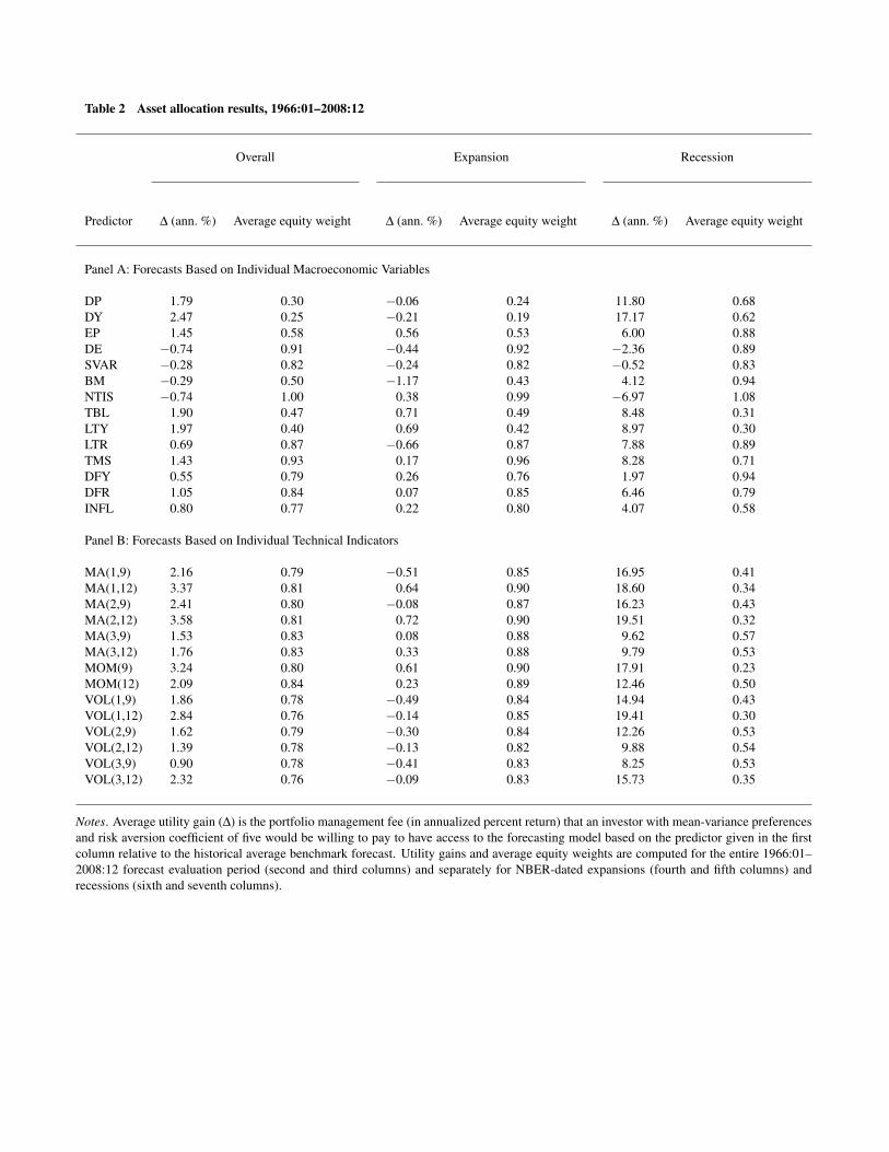
Table 2 Asset allocation results, 1966:01–2008:12

Overall Expansion Recession

Predictor ∆ (ann. %) Average equity weight ∆ (ann. %) Average equity weight ∆ (ann. %) Average equity weight

Panel A: Forecasts Based on Individual Macroeconomic Variables

DP 1.79 0.30 −0.06 0.24 11.80 0.68DY 2.47 0.25 −0.21 0.19 17.17 0.62EP 1.45 0.58 0.56 0.53 6.00 0.88DE −0.74 0.91 −0.44 0.92 −2.36 0.89SVAR −0.28 0.82 −0.24 0.82 −0.52 0.83BM −0.29 0.50 −1.17 0.43 4.12 0.94NTIS −0.74 1.00 0.38 0.99 −6.97 1.08TBL 1.90 0.47 0.71 0.49 8.48 0.31LTY 1.97 0.40 0.69 0.42 8.97 0.30LTR 0.69 0.87 −0.66 0.87 7.88 0.89TMS 1.43 0.93 0.17 0.96 8.28 0.71DFY 0.55 0.79 0.26 0.76 1.97 0.94DFR 1.05 0.84 0.07 0.85 6.46 0.79INFL 0.80 0.77 0.22 0.80 4.07 0.58

Panel B: Forecasts Based on Individual Technical Indicators

MA(1,9) 2.16 0.79 −0.51 0.85 16.95 0.41MA(1,12) 3.37 0.81 0.64 0.90 18.60 0.34MA(2,9) 2.41 0.80 −0.08 0.87 16.23 0.43MA(2,12) 3.58 0.81 0.72 0.90 19.51 0.32MA(3,9) 1.53 0.83 0.08 0.88 9.62 0.57MA(3,12) 1.76 0.83 0.33 0.88 9.79 0.53MOM(9) 3.24 0.80 0.61 0.90 17.91 0.23MOM(12) 2.09 0.84 0.23 0.89 12.46 0.50VOL(1,9) 1.86 0.78 −0.49 0.84 14.94 0.43VOL(1,12) 2.84 0.76 −0.14 0.85 19.41 0.30VOL(2,9) 1.62 0.79 −0.30 0.84 12.26 0.53VOL(2,12) 1.39 0.78 −0.13 0.82 9.88 0.54VOL(3,9) 0.90 0.78 −0.41 0.83 8.25 0.53VOL(3,12) 2.32 0.76 −0.09 0.83 15.73 0.35

Notes. Average utility gain (∆) is the portfolio management fee (in annualized percent return) that an investor with mean-variance preferencesand risk aversion coefficient of five would be willing to pay to have access to the forecasting model based on the predictor given in the firstcolumn relative to the historical average benchmark forecast. Utility gains and average equity weights are computed for the entire 1966:01–2008:12 forecast evaluation period (second and third columns) and separately for NBER-dated expansions (fourth and fifth columns) andrecessions (sixth and seventh columns).

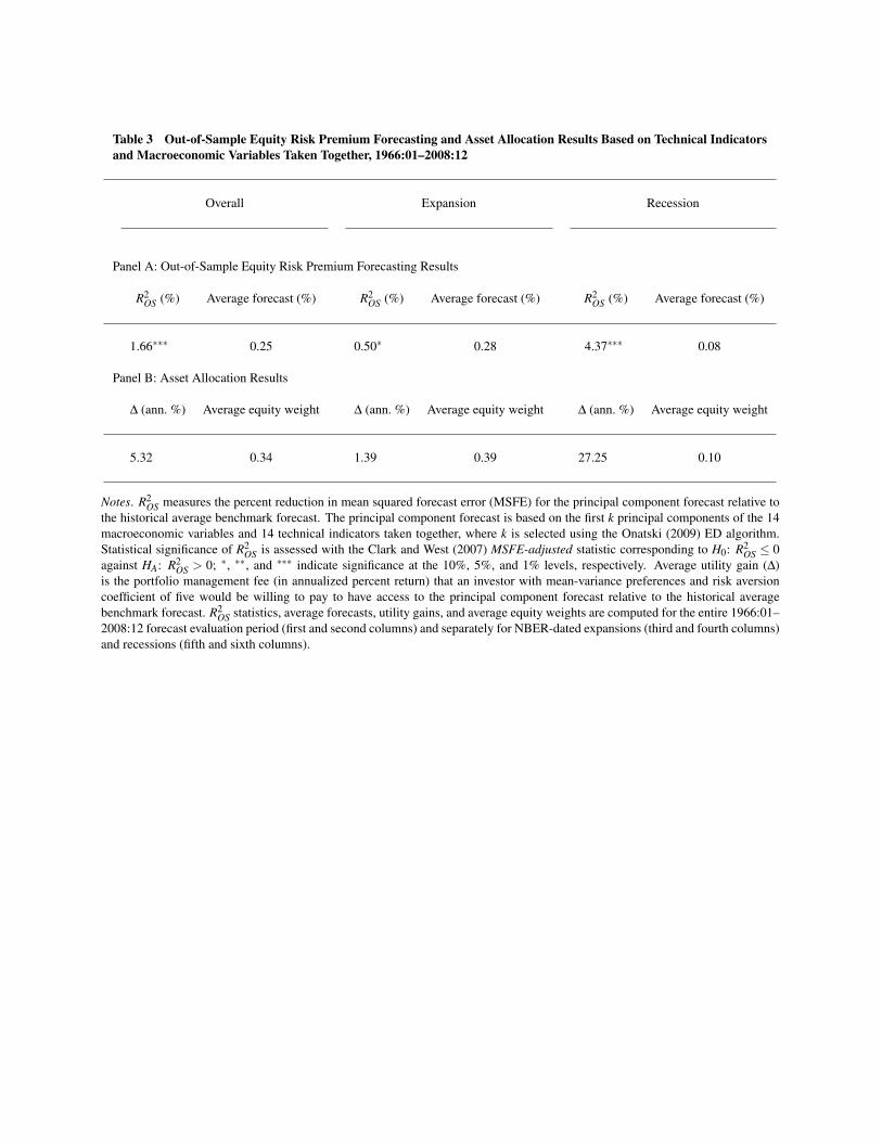
Table 3 Out-of-Sample Equity Risk Premium Forecasting and Asset Allocation Results Based on Technical Indicatorsand Macroeconomic Variables Taken Together, 1966:01–2008:12

Overall Expansion Recession

Panel A: Out-of-Sample Equity Risk Premium Forecasting Results

R2OS (%) Average forecast (%) R2

OS (%) Average forecast (%) R2OS (%) Average forecast (%)

1.66∗∗∗ 0.25 0.50∗ 0.28 4.37∗∗∗ 0.08

Panel B: Asset Allocation Results

∆ (ann. %) Average equity weight ∆ (ann. %) Average equity weight ∆ (ann. %) Average equity weight

5.32 0.34 1.39 0.39 27.25 0.10

Notes. R2OS measures the percent reduction in mean squared forecast error (MSFE) for the principal component forecast relative to

the historical average benchmark forecast. The principal component forecast is based on the first k principal components of the 14macroeconomic variables and 14 technical indicators taken together, where k is selected using the Onatski (2009) ED algorithm.Statistical significance of R2

OS is assessed with the Clark and West (2007) MSFE-adjusted statistic corresponding to H0: R2OS ≤ 0

against HA: R2OS > 0; ∗, ∗∗, and ∗∗∗ indicate significance at the 10%, 5%, and 1% levels, respectively. Average utility gain (∆)

is the portfolio management fee (in annualized percent return) that an investor with mean-variance preferences and risk aversioncoefficient of five would be willing to pay to have access to the principal component forecast relative to the historical averagebenchmark forecast. R2

OS statistics, average forecasts, utility gains, and average equity weights are computed for the entire 1966:01–2008:12 forecast evaluation period (first and second columns) and separately for NBER-dated expansions (third and fourth columns)and recessions (fifth and sixth columns).

Figure 1 Out-of-Sample Equity Risk Premium Forecasts Based on Individual Macroeconomic Variables, 1966:01–2008:12

1975 1985 1995 20050

0.5

1

1.5

2

DP

1975 1985 1995 20050

0.5

1

1.5

2

DY

1975 1985 1995 20050

0.5

1

1.5

2

EP

1975 1985 1995 20050

0.5

1

1.5

2

DE

1975 1985 1995 20050

0.5

1

1.5

2

SVAR

1975 1985 1995 20050

0.5

1

1.5

2

BM

1975 1985 1995 20050

0.5

1

1.5

2

NTIS

1975 1985 1995 20050

0.5

1

1.5

2

TBL

1975 1985 1995 20050

0.5

1

1.5

2

LTY

1975 1985 1995 20050

0.5

1

1.5

2

LTR

1975 1985 1995 20050

0.5

1

1.5

2

TMS

1975 1985 1995 20050

0.5

1

1.5

2

DFY

1975 1985 1995 20050

0.5

1

1.5

2

DFR

1975 1985 1995 20050

0.5

1

1.5

2

INFL

Notes. Black (gray) lines delineate equity risk premium forecasts in percent based on the macroeconomic variable given in the panel heading (historical average). Vertical bars depictNBER-dated recessions.

Figure 2 Cumulative Squared Forecast Error Differences, Out-of-Sample Equity Risk Premium Forecasts Based on the Historical Average and Individual MacroeconomicVariables, 1966:01–2008:12

1975 1985 1995 2005−0.02

−0.01

0

0.01

DP

1975 1985 1995 2005−0.02

−0.01

0

0.01

DY

1975 1985 1995 2005−0.02

−0.01

0

0.01

EP

1975 1985 1995 2005−0.02

−0.01

0

0.01

DE

1975 1985 1995 2005−0.02

−0.01

0

0.01

SVAR

1975 1985 1995 2005−0.02

−0.01

0

0.01

BM

1975 1985 1995 2005−0.02

−0.01

0

0.01

NTIS

1975 1985 1995 2005−0.02

−0.01

0

0.01

TBL

1975 1985 1995 2005−0.02

−0.01

0

0.01

LTY

1975 1985 1995 2005−0.02

−0.01

0

0.01

LTR

1975 1985 1995 2005−0.02

−0.01

0

0.01

TMS

1975 1985 1995 2005−0.02

−0.01

0

0.01

DFY

1975 1985 1995 2005−0.02

−0.01

0

0.01

DFR

1975 1985 1995 2005−0.02

−0.01

0

0.01

INFL

Notes. The figure depicts cumulative differences between squared forecast errors for the historical average equity risk premium forecast and the equity risk premium forecast based on themacroeconomic variable given in the panel heading. Vertical bars depict NBER-dated recessions.

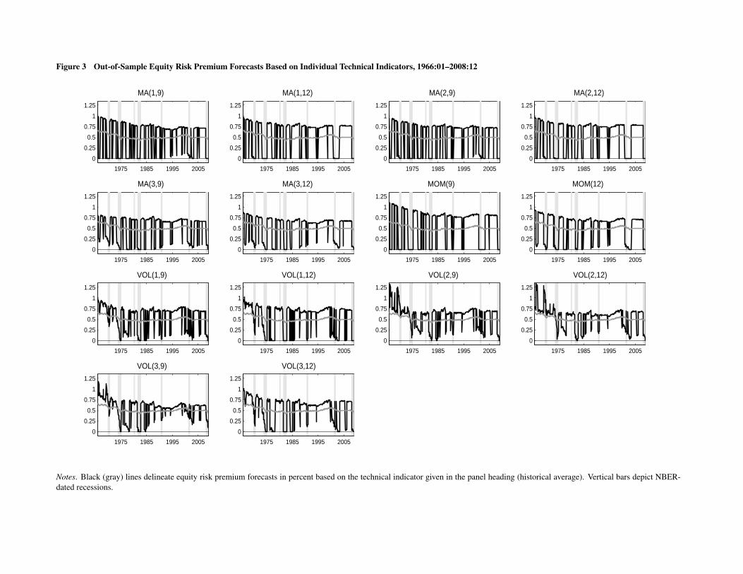
Figure 3 Out-of-Sample Equity Risk Premium Forecasts Based on Individual Technical Indicators, 1966:01–2008:12

1975 1985 1995 2005

0

0.25

0.5

0.75

1

1.25

MA(1,9)

1975 1985 1995 2005

0

0.25

0.5

0.75

1

1.25

MA(1,12)

1975 1985 1995 2005

0

0.25

0.5

0.75

1

1.25

MA(2,9)

1975 1985 1995 2005

0

0.25

0.5

0.75

1

1.25

MA(2,12)

1975 1985 1995 2005

0

0.25

0.5

0.75

1

1.25

MA(3,9)

1975 1985 1995 2005

0

0.25

0.5

0.75

1

1.25

MA(3,12)

1975 1985 1995 2005

0

0.25

0.5

0.75

1

1.25

MOM(9)

1975 1985 1995 2005

0

0.25

0.5

0.75

1

1.25

MOM(12)

1975 1985 1995 2005

0

0.25

0.5

0.75

1

1.25

VOL(1,9)

1975 1985 1995 2005

0

0.25

0.5

0.75

1

1.25

VOL(1,12)

1975 1985 1995 2005

0

0.25

0.5

0.75

1

1.25

VOL(2,9)

1975 1985 1995 2005

0

0.25

0.5

0.75

1

1.25

VOL(2,12)

1975 1985 1995 2005

0

0.25

0.5

0.75

1

1.25

VOL(3,9)

1975 1985 1995 2005

0

0.25

0.5

0.75

1

1.25

VOL(3,12)

Notes. Black (gray) lines delineate equity risk premium forecasts in percent based on the technical indicator given in the panel heading (historical average). Vertical bars depict NBER-dated recessions.

Figure 4 Cumulative squared forecast error differences, out-of-sample equity risk premium forecasts based on the historical average and individual technical indicators,1966:01–2008:12

1975 1985 1995 2005−0.01

−0.005

0

0.005

0.01

MA(1,9)

1975 1985 1995 2005−0.01

−0.005

0

0.005

0.01

MA(1,12)

1975 1985 1995 2005−0.01

−0.005

0

0.005

0.01

MA(2,9)

1975 1985 1995 2005−0.01

−0.005

0

0.005

0.01

MA(2,12)

1975 1985 1995 2005−0.01

−0.005

0

0.005

0.01

MA(3,9)

1975 1985 1995 2005−0.01

−0.005

0

0.005

0.01

MA(3,12)

1975 1985 1995 2005−0.01

−0.005

0

0.005

0.01

MOM(9)

1975 1985 1995 2005−0.01

−0.005

0

0.005

0.01

MOM(12)

1975 1985 1995 2005−0.01

−0.005

0

0.005

0.01

VOL(1,9)

1975 1985 1995 2005−0.01

−0.005

0

0.005

0.01

VOL(1,12)

1975 1985 1995 2005−0.01

−0.005

0

0.005

0.01

VOL(2,9)

1975 1985 1995 2005−0.01

−0.005

0

0.005

0.01

VOL(2,12)

1975 1985 1995 2005−0.01

−0.005

0

0.005

0.01

VOL(3,9)

1975 1985 1995 2005−0.01

−0.005

0

0.005

0.01

VOL(3,12)

Notes. The figure depicts cumulative differences between squared forecast errors for the historical average equity risk premium forecast and the equity risk premium forecast based on thetechnical indicator given in the panel heading. Vertical bars depict NBER-dated recessions.

Figure 5 Equity Portfolio Weights Computed Using Equity Risk Premium Forecasts Based on Individual Macroeconomic Variables, 1966:01–2008:12

1975 1985 1995 2005

0

0.5

1

1.5

DP

1975 1985 1995 2005

0

0.5

1

1.5

DY

1975 1985 1995 2005

0

0.5

1

1.5

EP

1975 1985 1995 2005

0

0.5

1

1.5

DE

1975 1985 1995 2005

0

0.5

1

1.5

SVAR

1975 1985 1995 2005

0

0.5

1

1.5

BM

1975 1985 1995 2005

0

0.5

1

1.5

NTIS

1975 1985 1995 2005

0

0.5

1

1.5

TBL

1975 1985 1995 2005

0

0.5

1

1.5

LTY

1975 1985 1995 2005

0

0.5

1

1.5

LTR

1975 1985 1995 2005

0

0.5

1

1.5

TMS

1975 1985 1995 2005

0

0.5

1

1.5

DFY

1975 1985 1995 2005

0

0.5

1

1.5

DFR

1975 1985 1995 2005

0

0.5

1

1.5

INFL

Notes. Black (gray) lines delineate equity portfolio weights for an investor with mean-variance preferences and risk aversion coefficient of five who uses an equity risk premium forecastbased on the macroeconomic variable given in the panel heading (historical average forecast). Vertical bars depict NBER-dated recessions.

Figure 6 Equity Portfolio Weights Computed Using Equity Risk Premium Forecasts Based on Individual Technical Indicators, 1966:01–2008:12

1975 1985 1995 2005

0

0.5

1

1.5

MA(1,9)

1975 1985 1995 2005

0

0.5

1

1.5

MA(1,12)

1975 1985 1995 2005

0

0.5

1

1.5

MA(2,9)

1975 1985 1995 2005

0

0.5

1

1.5

MA(2,12)

1975 1985 1995 2005

0

0.5

1

1.5

MA(3,9)

1975 1985 1995 2005

0

0.5

1

1.5

MA(3,12)

1975 1985 1995 2005

0

0.5

1

1.5

MOM(9)

1975 1985 1995 2005

0

0.5

1

1.5

MOM(12)

1975 1985 1995 2005

0

0.5

1

1.5

VOL(1,9)

1975 1985 1995 2005

0

0.5

1

1.5

VOL(1,12)

1975 1985 1995 2005

0

0.5

1

1.5

VOL(2,9)

1975 1985 1995 2005

0

0.5

1

1.5

VOL(2,12)

1975 1985 1995 2005

0

0.5

1

1.5

VOL(3,9)

1975 1985 1995 2005

0

0.5

1

1.5

VOL(3,12)

Notes. Black (gray) lines delineate equity portfolio weights for an investor with mean-variance preferences and risk aversion coefficient of five who uses an equity risk premium forecastbased on the technical indicator given in the panel heading (historical average forecast). Vertical bars depict NBER-dated recessions.

Figure 7 Actual Equity Risk Premium and Equity Risk Premium Forecasts Based on Individual Macroeconomic Variables Near a U.S. Business-Cycle Peak

−2 −1 0 1 2 3 4

−6

−3

0

3

6Actual

−2 −1 0 1 2 3 4

−0.6

−0.3

0

0.3

0.6

DP

−2 −1 0 1 2 3 4

−0.6

−0.3

0

0.3

0.6

DY

−2 −1 0 1 2 3 4

−0.6

−0.3

0

0.3

0.6

EP

−2 −1 0 1 2 3 4

−0.6

−0.3

0

0.3

0.6

DE

−2 −1 0 1 2 3 4

−0.6

−0.3

0

0.3

0.6

SVAR

−2 −1 0 1 2 3 4

−0.6

−0.3

0

0.3

0.6

BM

−2 −1 0 1 2 3 4

−0.6

−0.3

0

0.3

0.6

NTIS

−2 −1 0 1 2 3 4

−0.6

−0.3

0

0.3

0.6

TBL

−2 −1 0 1 2 3 4

−0.6

−0.3

0

0.3

0.6

LTY

−2 −1 0 1 2 3 4

−0.6

−0.3

0

0.3

0.6

LTR

−2 −1 0 1 2 3 4

−0.6

−0.3

0

0.3

0.6

TMS

−2 −1 0 1 2 3 4

−0.6

−0.3

0

0.3

0.6

DFY

−2 −1 0 1 2 3 4

−0.6

−0.3

0

0.3

0.6

DFR

−2 −1 0 1 2 3 4

−0.6

−0.3

0

0.3

0.6

INFL

Notes. The panels show the incremental change in the average difference between the actual equity risk premium or equity risk premium forecast based on the macroeconomic variablegiven in the panel heading and the historical average equity risk premium forecast two months before through four months after an NBER-dated peak. Actual and forecast values aremeasured in percent. Circles indicate point estimates and shaded areas depict 90% confidence bands.

Figure 8 Actual Equity Risk Premium and Equity Risk Premium Forecasts Based on Individual Technical Indicators Near a U.S. Business-Cycle Peak

−2 −1 0 1 2 3 4

−6

−3

0

3

6Actual

−2 −1 0 1 2 3 4−0.9

−0.6

−0.3

0

0.3MA(1,9)

−2 −1 0 1 2 3 4−0.9

−0.6

−0.3

0

0.3MA(1,12)

−2 −1 0 1 2 3 4−0.9

−0.6

−0.3

0

0.3MA(2,9)

−2 −1 0 1 2 3 4−0.9

−0.6

−0.3

0

0.3MA(2,12)

−2 −1 0 1 2 3 4−0.9

−0.6

−0.3

0

0.3MA(3,9)

−2 −1 0 1 2 3 4−0.9

−0.6

−0.3

0

0.3MA(3,12)

−2 −1 0 1 2 3 4−0.9

−0.6

−0.3

0

0.3MOM(9)

−2 −1 0 1 2 3 4−0.9

−0.6

−0.3

0

0.3MOM(12)

−2 −1 0 1 2 3 4−0.9

−0.6

−0.3

0

0.3VOL(1,9)

−2 −1 0 1 2 3 4−0.9

−0.6

−0.3

0

0.3VOL(1,12)

−2 −1 0 1 2 3 4−0.9

−0.6

−0.3

0

0.3VOL(2,9)

−2 −1 0 1 2 3 4−0.9

−0.6

−0.3

0

0.3VOL(2,12)

−2 −1 0 1 2 3 4−0.9

−0.6

−0.3

0

0.3VOL(3,9)

−2 −1 0 1 2 3 4−0.9

−0.6

−0.3

0

0.3VOL(3,12)

Notes. The panels show the incremental change in the average difference between the actual equity risk premium or equity risk premium forecast based on the technical indicator given inthe panel heading and the historical average equity risk premium forecast two months before through four months after an NBER-dated peak. Actual and forecast values are measured inpercent. Circles indicate point estimates and shaded areas depict 90% confidence bands.

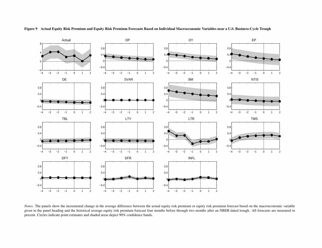
Figure 9 Actual Equity Risk Premium and Equity Risk Premium Forecasts Based on Individual Macroeconomic Variables near a U.S. Business-Cycle Trough

−4 −3 −2 −1 0 1 2−4

0

4

8Actual

−4 −3 −2 −1 0 1 2

−0.4

0

0.4

0.8

DP

−4 −3 −2 −1 0 1 2

−0.4

0

0.4

0.8

DY

−4 −3 −2 −1 0 1 2

−0.4

0

0.4

0.8

EP

−4 −3 −2 −1 0 1 2

−0.4

0

0.4

0.8

DE

−4 −3 −2 −1 0 1 2

−0.4

0

0.4

0.8

SVAR

−4 −3 −2 −1 0 1 2

−0.4

0

0.4

0.8

BM

−4 −3 −2 −1 0 1 2

−0.4

0

0.4

0.8

NTIS

−4 −3 −2 −1 0 1 2

−0.4

0

0.4

0.8

TBL

−4 −3 −2 −1 0 1 2

−0.4

0

0.4

0.8

LTY

−4 −3 −2 −1 0 1 2

−0.4

0

0.4

0.8

LTR

−4 −3 −2 −1 0 1 2

−0.4

0

0.4

0.8

TMS

−4 −3 −2 −1 0 1 2

−0.4

0

0.4

0.8

DFY

−4 −3 −2 −1 0 1 2

−0.4

0

0.4

0.8

DFR

−4 −3 −2 −1 0 1 2

−0.4

0

0.4

0.8

INFL

Notes. The panels show the incremental change in the average difference between the actual equity risk premium or equity risk premium forecast based on the macroeconomic variablegiven in the panel heading and the historical average equity risk premium forecast four months before through two months after an NBER-dated trough. All forecasts are measured inpercent. Circles indicate point estimates and shaded areas depict 90% confidence bands.

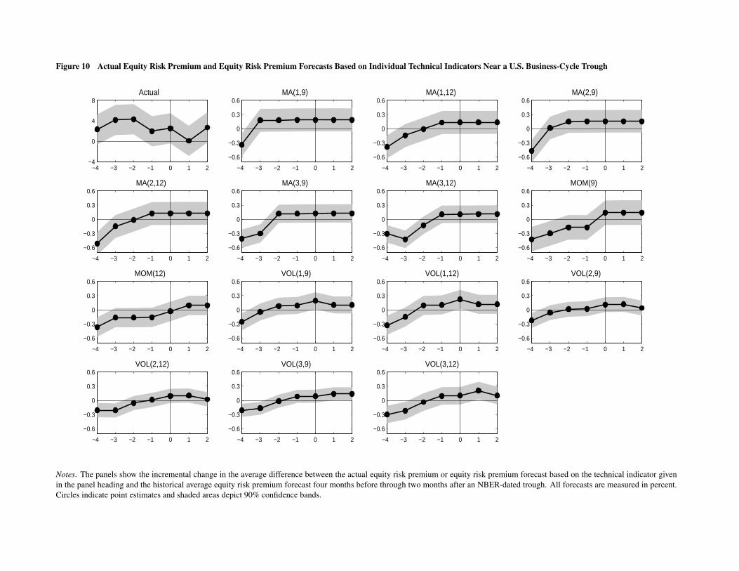
Figure 10 Actual Equity Risk Premium and Equity Risk Premium Forecasts Based on Individual Technical Indicators Near a U.S. Business-Cycle Trough

−4 −3 −2 −1 0 1 2−4

0

4

8Actual

−4 −3 −2 −1 0 1 2

−0.6

−0.3

0

0.3

0.6MA(1,9)

−4 −3 −2 −1 0 1 2

−0.6

−0.3

0

0.3

0.6MA(1,12)

−4 −3 −2 −1 0 1 2

−0.6

−0.3

0

0.3

0.6MA(2,9)

−4 −3 −2 −1 0 1 2

−0.6

−0.3

0

0.3

0.6MA(2,12)

−4 −3 −2 −1 0 1 2

−0.6

−0.3

0

0.3

0.6MA(3,9)

−4 −3 −2 −1 0 1 2

−0.6

−0.3

0

0.3

0.6MA(3,12)

−4 −3 −2 −1 0 1 2

−0.6

−0.3

0

0.3

0.6MOM(9)

−4 −3 −2 −1 0 1 2

−0.6

−0.3

0

0.3

0.6MOM(12)

−4 −3 −2 −1 0 1 2

−0.6

−0.3

0

0.3

0.6VOL(1,9)

−4 −3 −2 −1 0 1 2

−0.6

−0.3

0

0.3

0.6VOL(1,12)

−4 −3 −2 −1 0 1 2

−0.6

−0.3

0

0.3

0.6VOL(2,9)

−4 −3 −2 −1 0 1 2

−0.6

−0.3

0

0.3

0.6VOL(2,12)

−4 −3 −2 −1 0 1 2

−0.6

−0.3

0

0.3

0.6VOL(3,9)

−4 −3 −2 −1 0 1 2

−0.6

−0.3

0

0.3

0.6VOL(3,12)

Notes. The panels show the incremental change in the average difference between the actual equity risk premium or equity risk premium forecast based on the technical indicator givenin the panel heading and the historical average equity risk premium forecast four months before through two months after an NBER-dated trough. All forecasts are measured in percent.Circles indicate point estimates and shaded areas depict 90% confidence bands.

Figure 11 Out-of-Sample Equity Risk Premium Forecasts Based on Macroeconomic Variables and Technical Indicators Taken Together, 1966:01–2008:12

1970 1975 1980 1985 1990 1995 2000 2005

0

0.5

1

1.5

Principal component and historical average forecasts (%)

1970 1975 1980 1985 1990 1995 2000 2005−0.01

0

0.01

0.02

Difference in cumulative squared forecast error, historical average relative to principal component forecast

1970 1975 1980 1985 1990 1995 2000 2005

0

0.5

1

1.5

Equity weights based on principal component and historical average forecasts

Notes. Black (gray) line in the top panel delineates the principal component (historical average) equity risk premium forecast. The principal component (PC) equity risk premium forecastis based on the first k principal components of the 14 macroeconomic variables and 14 technical indicators taken together, where k is selected using the Onatski (2009) ED algorithm. Themiddle panel depicts cumulative differences between the squared forecast errors for the historical average and PC equity risk premium forecasts. Black (gray) line in the bottom paneldelineates the equity portfolio weight for an investor with mean-variance preferences and risk aversion coefficient of five who uses the PC equity risk premium forecast (historical averageforecast). Vertical bars depict NBER-dated recessions.