Forecasting the Demand of Oil in Ghana: A Statistical Approach

Management Science and Business Decisions

ISSN 2767-6528 / eISSN 2767-3316

2021 Volume 1 Issue 1: 29–43

https://doi.org/10.52812/msbd.25

Creative Commons Attribution-NonCommercial 4.0 International 29 © 2021 Science Insight

Forecasting the Demand of Oil in Ghana:

A Statistical Approach

Valentina Boamah1,*

1 School of Business, Nanjing University of Information Science and Technology, Nanjing, China

*Corresponding author:

Received 30 June 2021; Revised 6 July 2021; Accepted 7 July 2021

Abstract: Oil plays a vital role in the economic growth and sustainability of industries and their corporations. The

current study sought to forecast oil demand in Ghana for the next decade. The variables analyzed in this study were

Petroleum and other liquids, motor gasoline, distillate fuel, and liquefied petroleum gases (LPG). The study utilized

three univariate models; thus, linear regression, exponential regression, and exponential smoothing for forecasting

various oil components. The linear regression model was deemed a better fit for the analysis of most of the variables.

Furthermore, the findings revealed that the LPG growth rate is faster and requires less time to double in numbers

than the other energy sources. Also, the exponential smoothing model was ineffective and inefficient. Overall, the

demand for oil components analyzed will follow an increasing pattern from 2017 to 2027.

Keywords: Forecasting; Oil demand; Oil consumption; Energy; Ghana Africa

1. Introduction

Merchants and dealers involved in the oil markets view global oil demand and its output forecasts as

essential instruments. Speculative and non-quantifiable variables have essential roles in evaluating short-

run price fluctuations on the spot and in future markets. Oil prices escalating will lead to oil-consuming

nations' economic contraction and inflation, adversely affecting the world economy. Otherwise, a sharp

drop in oil price might preclude the economic growth of the countries producing oil and thus create

political turmoil and civil upheaval (Chen et al., 2018).

Developing countries like Ghana, Nigeria, Ivory Coast, among others, sometimes struggle to meet

the demands of their citizens, and oil is a clear example of it. Bourgeois and technical components that

affected each end energy category over the past decade have increased Ghana's demand for crude oil

and refined petroleum products. Ghana's oil consumption has increased substantially, and this has

shaken many energy experts. The function of energy resources in satisfying, among others, the needs

of households, factories, transportation, and agriculture in any economy cannot be overplayed.

Multiple forms of energy sources are needed to meet the demand for lighting, cooking, generating

electricity, among many other uses. Ghana's energy demand exceeds energy supply (Mensah et al., 2016).

In Ghana's energy sector, light crude oil is the main energy source that powers the electricity output of

thermal plants, apart from natural gas. As a multifunctional energy source heavily consumed in most

countries, the oil helps multiple sectors of an economy. Due to it being a very significant form of energy

for all economies, oil production and consumption are inextricably related to industrialization,

sustainable development and economic growth.

Management Science and Business Decisions: Vol. 1, No. 1 Baomah (2021)

30

In 2016, the government of Ghana decided to launch a new policy which stated one district, one

factory. With such expansion and development, the country will be aiming at growing its economy. Still,

the demand for oil will increase due to the industrialization tactics being adopted to implement such a

policy. With the amount of oil consumed significantly increasing and thus affecting the economic

growth of Ghana in the process, the data from the US EIA International Energy Statistics database

shows that there have been some variations in oil consumption values in Ghana since 2003 (see Figure

1).

From Figure 1, Petroleum and Other Liquid consumption reached its highest peak in 2017 with an

amount of 88TBPD (Total Barrels Per Day) and its lowest peak of 39TBPD in 2003. Motor Gasoline

consumption can also be seen experiencing variations in its values, reaching its highest peaks of

27TBPD in 2013, 2015 and 2017. Jet Fuel consumption, Residual Fuel Oil consumption and Liquefied

Petroleum Gases consumption (LPG) also reached their highest peak in 2017 with values of 4TBPD,

2TBPD, and 9TBPD, respectively. Kerosene consumption, Distillate Fuel Oil consumption, and Other

Refined Products consumption also had recorded values of 3.6TBPD, 39TBPD and 14TBPD,

respectively, as their highest peak in the years 2008, 2015 and 2016, respectively.

This study aims to forecast oil demand in Ghana for the next ten years, taking into account the

intensifying nature of oil demand in Ghana. To examine the amount of oil consumed in Ghana annually

and estimate the dynamics of the various types of oil that influence the aggregate oil demand in Ghana

are the key objectives operationalized from the main aim of this study. The subsequent sections of this

study are arranged as follows: Section 2 delves into the literature review highlighting underlying concepts

used to perform this study. Section 3 outlines the research methodology and approach, whilst sections

4 and 5 deals with results and discussions and, finally, the study concludes with recommendations.

2. Literature Review

Underlying works of literature that form the basis for conducting this research are discussed in this

section. The section describes the strengths and shortcomings of current literature based on the role of

oil in the energy sector in Ghana and oil forecasting, with key influencing factors affecting oil and its

demand in general.

2.1 The role of oil in Ghana's energy sector

"Supply chains are the veins of an economy" (Mahmoudi et al., 2021), and the energy sector enables

the smooth flow of supply in these veins. According to the world's economic and human development

indicators (HDI), the energy sector is a crucial component that drives economic growth and

development. The production and usage of oil can accelerate or impede economic growth as an essential

economic element. Over the last decade, oil demand has risen all over the world, leading to high prices.

Between 1980 and 2008, the price of crude oil fluctuated dramatically, with an average price of $32.31

(bbl), a minimum price of $12.72 (bbl) and a maximum price of $140 (bbl) respectively (Abledu et al.,

2013). A host of academic studies like that of Richardson et al. (2010), and Zhang et al. (2013) delved

into the increasing rate of energy demands or consumption for both developed and least developed

countries. The studies, as mentioned above, highlighted key determinants or indicators that culminate

into total consumption or extrapolated elements of various energy forms.

Ghana discovered oil in the year 2007. In 2010, the country began exploiting this resource, and the

country has realized its long-standing dream of improving its socio-economic growth with oil revenues

through subsequent discoveries. Ghana's energy sector has been prominent in numerous government

policies, such as initiatives to attain sustainable energy use to minimize the environmental impact,

increase access to new energy sources, and make energy products accessible and inexpensive for

Ghanaians (Mensah et al., 2016). A study by Ackah (2014) found that demand for natural gas is primarily

driven by income, population, prices, and industrial production share when it modelled Ghana's

aggregate residential and industrial demand for natural gas. But the the oil demand was not studied.

High growth rates of economic production and personal income are closely linked to the changing

oil requirements in Ghana. Increased demand for petrochemical feedstock, including naphtha-based

petrochemicals, which are close in composition to motor gasoline, drives the growth in production in

the industrial sector (Abledu et al., 2013). Duku et al. (2011) noted that Ghana's energy consumption

had increased significantly due to population growth and rapid urban growth. A continuing


31

Data source: International Energy Statistics, US EIA database

Graph source: Author's Construct Figure 1. Ghana's annual oil consumption between 2003 and 2017

Data source: International Energy Agency (IEA), 2020

Graph source: Author's Construct Figure 2. Ghana's energy supply between 1990 and 2018

Data source: International Energy Agency (IEA), 2020

Graph source: Author's Construct Figure 3. Ghana's oil consumption by sectors between 1990 and 2018

0

20

40

60

80

100

2003 2004 2005 2006 2007 2008 2009 2010 2011 2012 2013 2014 2015 2016 2017

Petroleum and Other Liquids Motor gasoline

Jet fuel Kerosene

Distillate fuel Residual fuel oil

0

1000

2000

3000

4000

5000

6000

7000

8000

9000

10000

1990 1992 1994 1996 1998 2000 2002 2004 2006 2008 2010 2012 2014 2016 2018

SUP

PLY

(K

TOE)

Hydro Biofuels and waste Oil

0

500

1000

1500

2000

2500

3000

3500

4000

1990 1992 1994 1996 1998 2000 2002 2004 2006 2008 2010 2012 2014 2016 2018

CO

NSU

MP

TIO

N (

KTO

E)

Industry TransportResidential Commercial and public servicesAgriculture/forestry


32

demographic shift from rural to urban areas drives the increase in incomes and the resulting changes in

oil demand. The rising urban population demands new vehicles and highways, thus increasing the

demand for oil in the transport sector.

2.2 Oil Forecasting

The significance of the energy sector and energy forecasts has not been sufficiently addressed for the

countries like Ghana. A vast amount of literature has been written about oil, determining the key

variables that affect it. Some of this literature takes a toll on forecasting the aggregate demand, whereas

some adopt the disaggregate demand for exploration. In empirical research, approaches based on the

ex-ante best individual forecasting model are effective, but on average, forecast combinations have been

found to generate effective forecasts (Timmermann, 2006).

Forecasting of oil demand and supply plays an essential role in a country's development agenda.

Several models have been used in the existing literature by several scholars, researchers and

organizations to make short, medium, and long-term projections. Notwithstanding these, there is no

specific forecasting model assigned to forecasters. However, some researchers commonly use some

existing standard forecasting models to make projections that have yielded the needed results. Hence,

standard forecasting models could be selected based on a researcher's objectives and the results the

researcher seeks to achieve. Such instances include Li et al. (2018) who developed 26 combination

models using the traditional combination method to avoid overfitting and increase prediction accuracy.

Furthermore, Wang et al. (2011) used the Hubbert and Generalized Weng models to provide them with

the basis for the empirical analysis of the variable they analyzed in their study. Also, Carlevaro et al.

(1989) modelled and forecasted the world demand for oil on a regional basis in the short – run using a

dynamic demand model. They concluded that their model deserved more changes to generate valuable

forecasts for the oil industry. As such, several existing forecasting models require further revision.

Owing to the fact that some unaccounted factors interfere with the actual values of oil, during

forecasting based on historical data, the actual value sometimes varies from the forecasted value.

Comparing the forecasted value with the actual value produces the measured error if there's any.

Therefore, some studies proposed that the mean absolute scaled error should be the standard accuracy

measure for comparing forecast accuracy over collective time series. To confirm the effectiveness of

their approach, Wang et al. (2018) evaluated their models using mean absolute error (MAE), mean

absolute percentage error (MAPE), and root mean square error (RMSE).

Table 1. Summary of oil forecast related literature

Year Country of focus Variable of forecast Methodology Literature

2009

United States, Canada, Japan,

Australia

Oil consumption

flexible fuzzy regression algorithm

Azadeh et al. (2009)

2009 Global Oil production Probabilistic estimate Kontorovich (2009)

2009 China Transport energy demand

PLSR Zhang et al. (2009)

2012

China Petroleum product consumption

Bayesian linear regression theory and

MCMC

Chai et al. (2012)

2012 Iran Transport energy demand

MLGP Forouzanfar et al. (2012)

2013 Global Oil demand STSM Suleiman (2013)

2015

Nigeria

Oil production

M.A., SES, AF, Box-Jenkings, Classical Decomposition

Aideyan & Nima (2015)

2015 OPEC Oil production Multi–cyclic Hubbert Model

Ebrahimi & Ghasabani (2015)

2015 U.K., Norway Oil production Monte – Carlo method

Fiévet et al. (2015)

2019 China Oil demand STSM Fatima et al. (2019)

2019 India Foreign oil NMGM-ARIMA and NMGM-BP

Li & Wang (2019)

2021 Ghana Oil demand LR, ER and ETS The current study PLSR partial least square regression, M.A. moving average, SES seasonal exponential smoothing, A.F. adaptive filtering, MCMC Markov Chain Monte Carlo method, MLGP multi-level genetic programming, STSM structural time series model, NMGM-ARIMA nonlinear metabolic grey model – linear autoregressive integrated moving average and NMGM-BP nonlinear metabolic grey model - nonlinear backpropagation, LR Linear regression, ER exponential regression, ETS exponential smoothing


33

Cheze et al. (2011) forecasted jet fuel consumption at the worldwide level and eight geographical

zones by 2025 using dynamic panel–data econometrics. Their findings revealed that between 2008 and

2025, the world's air traffic would increase by 100%, with a growth rate of 4.7% annually. Moreover,

the estimated demand of the world for jet fuel will increase by approximately 38%, with an average

growth rate of 1.9% annually. Al-Yousef (2004), in his study, proposed a model to predict crude oil

consumption for some Asian countries over the period 1982 – 2002. He concluded that GDP and price

are important factors in oil demand. He also added that growth in GDP is an important element in the

growth or fall in Asian countries' demand for crude oil. Due to briefness, table 1 contains other studies

conducted by researchers about the forecasting of oil.

3. Research Methodology

This section focuses on the methodology and approach adopted in the current study for forecasting

the demand for oil in Ghana for the next decade based on time series data. The study adopted three

univariate models; linear regression model, exponential regression model, and exponential smoothing

model. Microsoft Excel (2016 version) was used to run the models.

3.1 Data collection

The bp Statistical Review of World Energy (BP, 2020) ranked oil as the largest share of the energy

mix, accounting for 33.1% and perhaps being a dominant economic growth tool in Africa. It also

recorded 4096 thousand barrels per day as the consumption of oil in the whole of Africa. The current

study sampled 15 years (2003 to 2017) time-series data of Ghana's annual oil consumption. Data from

2003 to 2015 was used for forecasting, and the 2016-2017 data was used for out-of-sample testing. The

four energy sources were considered for forecasting; petroleum and other liquids, motor gasoline,

distillate fuel oil, and liquefied petroleum gas (LPG). The oil consumption data set was gathered from

the U.S. Energy Information Administration (www.eia.gov).

For the study to gain an insight into the vast reach of oil in Ghana, data pertaining to Ghana's energy

sector for the period 1990 to 2018 were also gathered. Ghana's energy supply and Ghana's oil

consumption by sectors data were obtained from the International Energy Agency (www.iea.org) for

this exploration. Data availability was the justification for choosing the period (1990 to 2018).

3.2 Forecasting Techniques

Descriptively, forecasting is carried out by testing time series data with a developed model or applying

technical approaches. Over specific periods, distinct models have been tried to predict data, and

accurate calculations are needed to determine the accuracy of such models. Time series models used for

forecasting can be classified into univariate and multivariate models (Tularam & Saeed 2016). In order

to predict the values of a variable that acts as a response variable, univariate data analysis involves the

use of past data and involves a distinct evaluation of the findings for each variable in the given data.

Thus, the univariate analysis does not find the causation or correlation relationship between

independent variables. This study adopted the univariate models, namely; linear regression models,

exponential models and exponential smoothing models, for forecasting oil demand in Ghana for a

decade. These models were selected due to (1) they are a widely used form of forecasting and (2) the

characteristics the data used in this study possess.

3.2.1 Linear regression model. A linear regression (LR) model is a simple yet widely used form of

forecasting. The model forms a linear relationship between the forecast variable F and the single

explanatory variable Y. In order to analyze the relationship between the variables, the model is defined

as:

𝐹𝑡 = 𝛽0 + 𝛽1𝑌𝑡 + 𝜀

where,

𝛽0 = the intercept

𝛽1 = the slope of the line


34

𝐹𝑡 = forecasted value for year t

𝑌𝑡 = Year t

𝜀 = the error term

The intercept 𝛽0 represents the forecasted value of 𝐹𝑡 when the explanatory variable (𝑌𝑡 )= 0. And

the slope of the line 𝛽1 represents the average predicted change in the forecasted value F_t resulting

from a one-unit increase or decrease in the explanatory variable 𝑌𝑡. For further details, Sarstedt and

Mooi (2014) can be consulted. In the current study, Microsoft Excel's built-in function was used for

linear regression.

3.2.2 Exponential regression model. An exponential regression (ER) model is a nonlinear form of a

regression model. It is used to model data that does not follow a linear pattern. Exponential regression

is used to predict conditions in which development starts slowly and then elevates quickly without

bounds or where decay begins speedily and then slows down to get closer and closer to zero. The model

is developed as follows:

𝐹𝑡 = 𝛽0𝑒𝛽1𝑌𝑡 + 𝜀

where,

𝐹𝑡 = forecasted value for year t

𝑌𝑡 = Year t.

The coefficients 𝛽0 and 𝛽1 are obtained from the graph (data). For further details, Davidov and Zelen

(2000) can be consulted. In the current study, Microsoft Excel's built-in function was used for

exponential regression.

3.2.3 Exponential Smoothing technique. The exponential smoothing model was first suggested in the late

1950s. This approach is acceptable for forecasting data without a specific trend or seasonal pattern. The

exponential smoothing model developed to examine the data is specified as:

𝐿0 = 1

𝑛∑ 𝐷𝑡

𝑛

𝑡=1

𝐹𝑡+1 = 𝐿𝑡

𝐿𝑡+1 = 𝛼𝐷𝑡+1 + (1 − 𝛼)𝐿𝑡

where,

𝑛 = number of years

𝐷𝑡 = actual demand at year t

𝐷𝑡+1 = current year's actual demand

𝐿0 = forecast demand for year 1

𝐿𝑡 = previous year's forecast demand

𝐿𝑡+1= current year's forecast demand

𝛼 = smoothing constant; 0 < 𝛼 < 1.

For further details, Chopra and Meindl (2015: Chapter 7) can be consulted. Microsoft Excel's built-

in function for exponential triple smoothing (ETS) was used in the current study.


35

3.3 Forecast Error Measurement

It has been widely recognized that forecasts are always inaccurate. Therefore, they should be

accompanied by both the expected value of the forecast and a measure of forecast error (Javed et al.,

2020b; Ofosu-Adarkwa et al., 2020). Following Javed et al. (2020a), the Mean Absolute Percentage Error

(MAPE) was used to test the performance of the forecasting techniques. The MAPE formula is denoted

by:

𝑀𝐴𝑃𝐸(%) = 1

𝑛∑ |

𝑥(𝑘) − �̂�(𝑘)

𝑥(𝑘)|

𝑛

𝑘=1

× 100%

where,

𝑥(𝑘) = actual values

�̂�(𝑘) = simulated values

𝑛 = number of years.

Table 2. Forecasting the consumption of petroleum and other liquids

Year Actual data LR ER ETS Cumulative RGR RGR (mean) Dt Dt (mean)

2003 39 34.83 35.28 47.09 39 -

2004 43 38.88 37.79 50.24 82 0.74 0.25 0.99 2.25

2005 44 42.92 40.48 53.38 126 0.43 1.54

2006 43 46.96 43.37 56.52 169 0.29 1.92

2007 48 51.01 46.46 59.66 217 0.25 2.08

2008 49 55.05 49.77 62.81 266 0.20 2.28

2009 58 59.10 53.31 65.95 324 0.20 2.32

2010 59 63.14 57.11 69.09 383 0.17 2.48

2011 67 67.18 61.17 72.23 450 0.16 2.52

2012 76 71.23 65.53 75.38 526 0.16 2.55

2013 77 75.27 70.20 78.52 603 0.14 2.68

2014 78 79.32 75.20 81.66 681 0.12 2.80

2015 86 83.36 80.55 84.80 767 0.12 2.82

2016 88 87.40 86.29 87.95 87.40 - -

2017 88 91.45 92.44 91.09 178.85 0.72 0.25 1.03 2.28

2018 95.49 99.02 94.23 274.34 0.43 1.54

2019 99.54 106.07 97.37 373.88 0.31 1.87

2020 103.58 113.63 100.52 477.46 0.24 2.10

2021 107.62 121.72 103.66 585.08 0.20 2.29

2022 111.67 130.39 106.80 696.75 0.17 2.44

2023 115.71 139.67 109.94 812.46 0.15 2.57

2024 119.76 149.62 113.09 932.22 0.14 2.68

2025 123.80 160.28 116.23 1056.02 0.12 2.78

2026 127.84 171.69 119.37 1183.86 0.11 2.86

2027 131.89 183.92 122.51 1315.75 0.11 2.94

MAPE (%) in- sample

5.62 6.75 14.64

MAPE (%) out-of-sample

2.30 3.49 1.79

NOTE: Actual data (2003 – 2015) and LR-based data (2016 – 2027) were used for the cumulative estimations.


36

The Lewis scale (Javed et al., 2020a) was used for interpreting the MAPE values:

𝑀𝐴𝑃𝐸(%) = {

< 10 𝐻𝑖𝑔ℎ𝑙𝑦 𝑎𝑐𝑐𝑢𝑟𝑎𝑡𝑒 𝑓𝑜𝑟𝑒𝑐𝑎𝑠𝑡10~20 𝐺𝑜𝑜𝑑 𝑓𝑜𝑟𝑒𝑐𝑎𝑠𝑡20~50 𝑅𝑒𝑎𝑠𝑜𝑛𝑎𝑏𝑙𝑒 𝑓𝑜𝑟𝑒𝑐𝑎𝑠𝑡

> 50 𝐼𝑛𝑎𝑐𝑐𝑢𝑟𝑎𝑡𝑒 𝑓𝑜𝑟𝑒𝑐𝑎𝑠𝑡

3.4 Growth Rate and Doubling Time Analyses

Growth rate and doubling time analyses make forecasts more useful for decision-makers. The

expression for the relative growth rate (𝑅𝐺𝑅) and doubling time (𝐷𝑡) are given by (Javed & Liu, 2018;

Quartey-Papafio et al., 2020):

𝑅𝐺𝑅 = (𝑙𝑛𝑁2 − 𝑙𝑛𝑁1)/(𝑡2 − 𝑡1)

Since in our study 𝑡2 − 𝑡1 is one, the equation is further deduced to:

𝑅𝐺𝑅 = 𝑙𝑛(𝑁2/𝑁1)

Table 3. Forecasting the consumption of motor gasoline

Year Actual data LR ER ETS Cumulative RGR RGR (mean) Dt Dt (mean)

2003 12 10.05 10.59 28.25 12 -

2004 14 11.47 11.42 28.25 26 0.77 0.25 0.95 2.24

2005 13 12.89 12.32 28.25 39 0.41 1.60

2006 13 14.31 13.29 28.25 52 0.29 1.94

2007 14 15.72 14.34 28.25 66 0.24 2.13

2008 14 17.14 15.47 28.24 80 0.19 2.34

2009 18 18.56 16.69 28.24 98 0.20 2.29

2010 18 19.98 18.01 28.24 116 0.17 2.47

2011 20 21.39 19.43 28.24 136 0.16 2.53

2012 25 22.81 20.96 28.24 161 0.17 2.47

2013 27 24.23 22.62 28.24 188 0.16 2.56

2014 26 25.65 24.40 28.24 214 0.13 2.74

2015 27 27.06 26.32 28.24 241 0.12 2.82

2016 25 28.48 28.40 28.24 28.40 - -

2017 27 29.90 30.64 28.23 59.04 0.73 0.27 1.01 2.17

2018 31.32 33.05 28.23 92.09 0.44 1.50

2019 32.73 35.66 28.23 127.75 0.33 1.81

2020 34.15 38.47 28.23 166.23 0.26 2.03

2021 35.57 41.51 28.23 207.74 0.22 2.19

2022 36.99 44.78 28.23 252.52 0.20 2.33

2023 38.40 48.31 28.23 300.83 0.18 2.44

2024 39.82 52.12 28.23 352.95 0.16 2.53

2025 41.24 56.23 28.23 409.18 0.15 2.60

2026 42.66 60.67 28.22 469.84 0.14 2.67

2027 44.08 65.45 28.22 535.29 0.13 2.73

MAPE (%) in- sample

9.35 7.83 66.23


12.33 13.54 8.76

NOTE: Actual data (2003 – 2015) and ER-based data (2016 – 2027) were used for the cumulative estimations.


37

The time needed for the variables analyzed to double in numbers for a given 𝑅𝐺𝑅 is measured by

the 𝐷𝑡 and this is denoted as:

𝐷𝑡 = (𝑡2 − 𝑡1) ln [2

𝑙𝑛𝑁2 − 𝑙𝑛𝑁1]

or,

𝐷𝑡 = 𝑙𝑛(2/𝑅𝐺𝑅)

where,

𝑁2 = analyzed variable's cumulative number in the year 𝑡2

𝑁1 = analyzed variable's cumulative number in the year 𝑡1

A general assessment of the variations of the different variables between the actual trend and the

expected trend is useful but challenging. The traditional 𝑅𝐺𝑅 and 𝐷𝑡 cannot solve the problem,

especially when the forecasted trend is different from the historical trend. Javed and Liu (2018) solved

this problem by introducing a system for estimating the Synthetic Relative Growth Rate (𝑅𝐺𝑅𝑠𝑦𝑛𝑡ℎ𝑒𝑡𝑖𝑐)

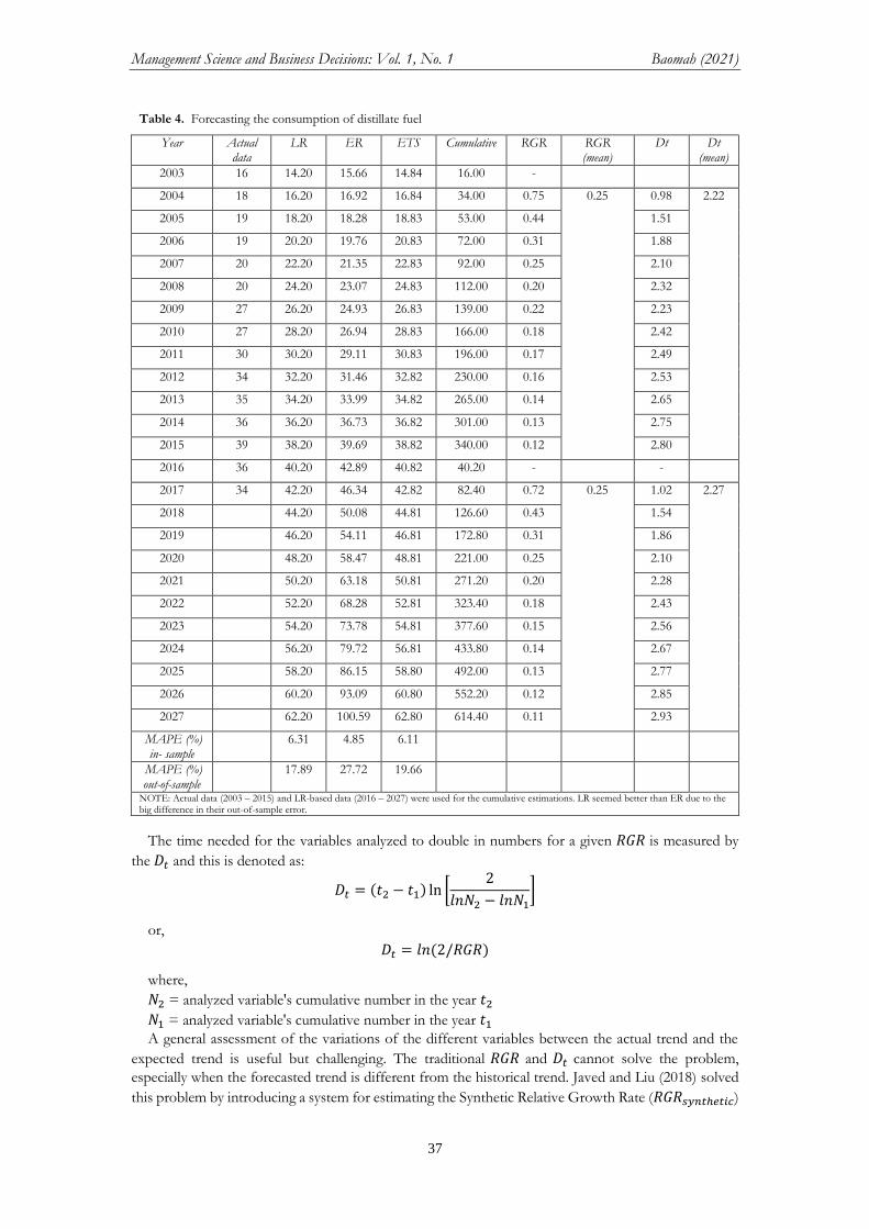
Table 4. Forecasting the consumption of distillate fuel

Year Actual data

LR ER ETS Cumulative RGR RGR (mean)

Dt Dt (mean)

2003 16 14.20 15.66 14.84 16.00 -

2004 18 16.20 16.92 16.84 34.00 0.75 0.25 0.98 2.22

2005 19 18.20 18.28 18.83 53.00 0.44 1.51

2006 19 20.20 19.76 20.83 72.00 0.31 1.88

2007 20 22.20 21.35 22.83 92.00 0.25 2.10

2008 20 24.20 23.07 24.83 112.00 0.20 2.32

2009 27 26.20 24.93 26.83 139.00 0.22 2.23

2010 27 28.20 26.94 28.83 166.00 0.18 2.42

2011 30 30.20 29.11 30.83 196.00 0.17 2.49

2012 34 32.20 31.46 32.82 230.00 0.16 2.53

2013 35 34.20 33.99 34.82 265.00 0.14 2.65

2014 36 36.20 36.73 36.82 301.00 0.13 2.75

2015 39 38.20 39.69 38.82 340.00 0.12 2.80

2016 36 40.20 42.89 40.82 40.20 - -

2017 34 42.20 46.34 42.82 82.40 0.72 0.25 1.02 2.27

2018 44.20 50.08 44.81 126.60 0.43 1.54

2019 46.20 54.11 46.81 172.80 0.31 1.86

2020 48.20 58.47 48.81 221.00 0.25 2.10

2021 50.20 63.18 50.81 271.20 0.20 2.28

2022 52.20 68.28 52.81 323.40 0.18 2.43

2023 54.20 73.78 54.81 377.60 0.15 2.56

2024 56.20 79.72 56.81 433.80 0.14 2.67

2025 58.20 86.15 58.80 492.00 0.13 2.77

2026 60.20 93.09 60.80 552.20 0.12 2.85

2027 62.20 100.59 62.80 614.40 0.11 2.93

MAPE (%) in- sample

6.31 4.85 6.11


17.89 27.72 19.66

NOTE: Actual data (2003 – 2015) and LR-based data (2016 – 2027) were used for the cumulative estimations. LR seemed better than ER due to the big difference in their out-of-sample error.


38

and Synthetic Doubling Time (𝐷𝑠𝑦𝑛𝑡ℎ𝑒𝑡𝑖𝑐). This approach effectively gives the overall picture of the

𝑅𝐺𝑅 and 𝐷𝑡. The formulas are given by;

𝑅𝐺𝑅𝑠𝑦𝑛𝑡ℎ𝑒𝑡𝑖𝑐 = 𝜃. (𝑅𝐺𝑅𝑎𝑐𝑡𝑢𝑎𝑙) + (1 − 𝜃). 𝑅𝐺𝑅𝑓𝑜𝑟𝑒𝑐𝑎𝑠𝑡

𝐷𝑠𝑦𝑛𝑡ℎ𝑒𝑡𝑖𝑐 = 𝜃. (𝐷𝑎𝑐𝑡𝑢𝑎𝑙) + (1 − 𝜃). 𝐷𝑓𝑜𝑟𝑒𝑐𝑎𝑠𝑡

where,

𝑅𝐺𝑅𝑎𝑐𝑡𝑢𝑎𝑙 = relative growth rate derived through actual data

𝑅𝐺𝑅𝑓𝑜𝑟𝑒𝑐𝑎𝑠𝑡 = relative growth rate derived through forecasted data

𝐷𝑎𝑐𝑡𝑢𝑎𝑙 = doubling time derived through actual data

𝐷𝑓𝑜𝑟𝑒𝑐𝑎𝑠𝑡 = relative growth rate derived through forecasted data

𝜃 = the weighing coefficient, valued at 0.5 in the current study

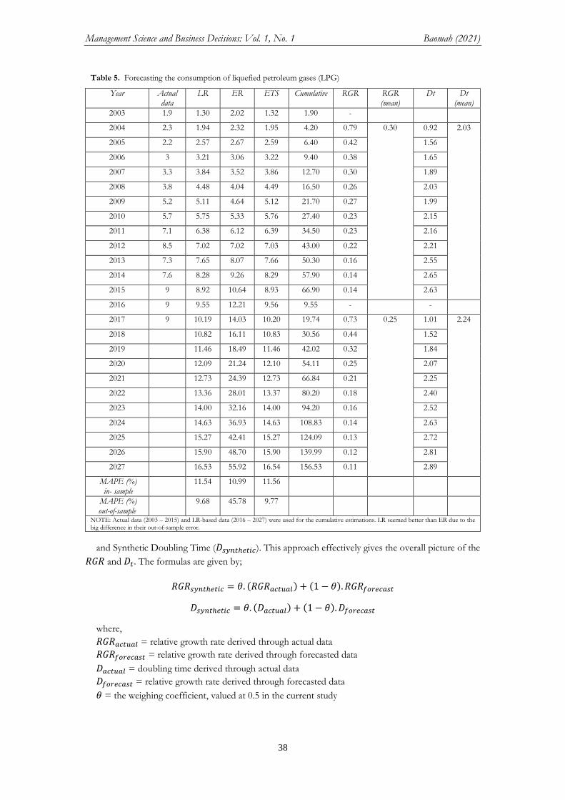
Table 5. Forecasting the consumption of liquefied petroleum gases (LPG)

Year Actual data

LR ER ETS Cumulative RGR RGR (mean)

Dt Dt (mean)

2003 1.9 1.30 2.02 1.32 1.90 -

2004 2.3 1.94 2.32 1.95 4.20 0.79 0.30 0.92 2.03

2005 2.2 2.57 2.67 2.59 6.40 0.42 1.56

2006 3 3.21 3.06 3.22 9.40 0.38 1.65

2007 3.3 3.84 3.52 3.86 12.70 0.30 1.89

2008 3.8 4.48 4.04 4.49 16.50 0.26 2.03

2009 5.2 5.11 4.64 5.12 21.70 0.27 1.99

2010 5.7 5.75 5.33 5.76 27.40 0.23 2.15

2011 7.1 6.38 6.12 6.39 34.50 0.23 2.16

2012 8.5 7.02 7.02 7.03 43.00 0.22 2.21

2013 7.3 7.65 8.07 7.66 50.30 0.16 2.55

2014 7.6 8.28 9.26 8.29 57.90 0.14 2.65

2015 9 8.92 10.64 8.93 66.90 0.14 2.63

2016 9 9.55 12.21 9.56 9.55 - -

2017 9 10.19 14.03 10.20 19.74 0.73 0.25 1.01 2.24

2018 10.82 16.11 10.83 30.56 0.44 1.52

2019 11.46 18.49 11.46 42.02 0.32 1.84

2020 12.09 21.24 12.10 54.11 0.25 2.07

2021 12.73 24.39 12.73 66.84 0.21 2.25

2022 13.36 28.01 13.37 80.20 0.18 2.40

2023 14.00 32.16 14.00 94.20 0.16 2.52

2024 14.63 36.93 14.63 108.83 0.14 2.63

2025 15.27 42.41 15.27 124.09 0.13 2.72

2026 15.90 48.70 15.90 139.99 0.12 2.81

2027 16.53 55.92 16.54 156.53 0.11 2.89

MAPE (%) in- sample

11.54 10.99 11.56


9.68 45.78 9.77

NOTE: Actual data (2003 – 2015) and LR-based data (2016 – 2027) were used for the cumulative estimations. LR seemed better than ER due to the big difference in their out-of-sample error.


39

For further details on relative growth rate and doubling time analyses and their synthetic versions,

Javed and Liu (2018) is recommended.

4. Results

Results obtained from analyzing the data used for this study are discussed in this chapter. The data

(2003-2017) were analyzed using Microsoft Excel 2016 version software. The periods 2016 and 2017

were used for out-of-sample testing. The linear regression models (LR), exponential regression models

(ER) and exponential smoothing models (ETS) were used to forecast for oil demand in Ghana over the

next ten years. The results of the analysis are summarized in Tables 2 to 5. The MAPE was estimated

to test the accuracy of the models. Relative growth rate (𝑅𝐺𝑅) and doubling time (𝐷𝑡) were also used

to analyze the growth of the variables explored in this study. Furthermore, the Synthetic Relative

Growth Rate (𝑅𝐺𝑅𝑠𝑦𝑛𝑡ℎ𝑒𝑡𝑖𝑐) and Synthetic Doubling Time (𝐷𝑠𝑦𝑛𝑡ℎ𝑒𝑡𝑖𝑐) were applied to assess the

variations of the different variables between the actual trend and the expected trend.

Table 2 provides the results obtained for the variable Petroleum and other liquids. Both the Linear

Regression and Exponential Regression provided highly accurate forecasts based on the MAPE scale

adopted for this study. The Linear Regression instead had a higher forecasting accuracy as compared to

the other models. The Linear Regression and Exponential Regression models developed for the

Petroleum and other liquids variable are 𝐹𝑡 = 4.044𝑌𝑡 − 8065.3 and 𝐹𝑡 = 5𝐸 − 59𝑒0.0688𝑌𝑡 ,

respectively.

Table 3 provides the results obtained for the variable Motor gasoline. After analyzing the data, the

results provided Linear Regression and Exponential Regression models 𝐹𝑡 = 1.4176𝑌𝑡 − 2829.4 and

𝐹𝑡 = 1𝐸 − 65𝑒0.0759𝑌𝑡, respectively. The application of the ETS model for forecasting was ineffective

for this variable. The Exponential Regression instead provided good forecasting results as compared to

the other models.

Table 4 provides the results obtained for the variable Distillate fuel. After analyzing the data, the

results provided Linear Regression and Exponential Regression models 𝐹𝑡 = 2𝑌𝑡 − 3991.8 and 𝐹𝑡 =

6𝐸 − 67𝑒0.0775𝑌𝑡, respectively. Although the application of all three of the forecasting models was

effective for this variable, Linear Regression seemed better than Exponential Regression in this case

because their out-of-sample errors had a big difference.

Table 5 provides the results obtained for the variable Liquefied Petroleum Gasses (LPG). After

analyzing the data, the results provided Linear Regression and Exponential Regression models 𝐹𝑡 =

0.6346𝑌𝑡 − 1269.8 and 𝐹𝑡 = 1𝐸 − 120𝑒0.1383𝑌𝑡 , respectively. Based on the comparison made

between the three models' MAPE values, Linear Regression seemed better than Exponential Regression

in this case because of the vast difference in their out-of-sample errors.

Moreover, the sequence obtained according to the 𝑅𝐺𝑅 based on the actual data are;

Liquified petroleum gases (LPG)0.297 > 𝐷𝑖𝑠𝑡𝑖𝑙𝑙𝑎𝑡𝑒 𝑓𝑢𝑒𝑙0.255 > 𝑀𝑜𝑡𝑜𝑟 𝑔𝑎𝑠𝑜𝑙𝑖𝑛𝑒0.25

> 𝑃𝑒𝑡𝑟𝑜𝑙𝑒𝑢𝑚 𝑎𝑛𝑑 𝑜𝑡ℎ𝑒𝑟 𝑙𝑖𝑞𝑢𝑖𝑑𝑠0.248

Moreover, the sequence obtained according to the 𝐷𝑡 based on the actual data are;

Liquified petroleum gases (LPG)2.033 < 𝐷𝑖𝑠𝑡𝑖𝑙𝑙𝑎𝑡𝑒 𝑓𝑢𝑒𝑙2.220 < 𝑀𝑜𝑡𝑜𝑟 𝐺𝑎𝑠𝑜𝑙𝑖𝑛𝑒2.236

< 𝑃𝑒𝑡𝑟𝑜𝑙𝑒𝑢𝑚 𝑎𝑛𝑑 𝑜𝑡ℎ𝑒𝑟 𝑙𝑖𝑞𝑢𝑖𝑑𝑠2.249

The above 𝑅𝐺𝑅 and 𝐷𝑡 provides insight into the relative growth rate for LPG and Distillate, which

is increasing compared to Motor gasoline and Petroleum and other liquids. Furthermore, for a given

𝑅𝐺𝑅, LPG and Distillate fuel need less time to double in numbers than Motor gasoline and Petroleum

and other liquids.

Also, the sequence obtained for the 𝑅𝐺𝑅𝑠𝑦𝑛𝑡ℎ𝑒𝑡𝑖𝑐 are;


40

Liquified petroleum gases (LPG)0.275 > 𝑀𝑜𝑡𝑜𝑟 𝐺𝑎𝑠𝑜𝑙𝑖𝑛𝑒0.258 > 𝐷𝑖𝑠𝑡𝑖𝑙𝑙𝑎𝑡𝑒 𝑓𝑢𝑒𝑙0.251

> 𝑃𝑒𝑡𝑟𝑜𝑙𝑒𝑢𝑚 𝑎𝑛𝑑 𝑜𝑡ℎ𝑒𝑟 𝑙𝑖𝑞𝑢𝑖𝑑𝑠0.247

And the sequence obtained for the 𝐷𝑠𝑦𝑛𝑡ℎ𝑒𝑡𝑖𝑐 are;

Liquified petroleum gases (LPG)2.2136 < 𝑀𝑜𝑡𝑜𝑟 𝐺𝑎𝑠𝑜𝑙𝑖𝑛𝑒2.201 < 𝐷𝑖𝑠𝑡𝑖𝑙𝑙𝑎𝑡𝑒 𝑓𝑢𝑒𝑙2.246

< 𝑃𝑒𝑡𝑟𝑜𝑙𝑒𝑢𝑚 𝑎𝑛𝑑 𝑜𝑡ℎ𝑒𝑟 𝑙𝑖𝑞𝑢𝑖𝑑𝑠2.264

According to the 𝑅𝐺𝑅𝑠𝑦𝑛𝑡ℎ𝑒𝑡𝑖𝑐 LPG's growth rate is increasing faster than Motor Gasoline,

Distillate fuel and Petroleum and Other liquids. Furthermore, LPG requires less time to double in

numbers according to the 𝐷𝑠𝑦𝑛𝑡ℎ𝑒𝑡𝑖𝑐 then the other variables.

Figure 4. The forecasted values against the actual values (Annual, TBPD)

0

50

100

150

200

20

03

20

05

20

07

20

09

20

11

20

13

20

15

20

17

20

19

20

21

20

23

20

25

20

27

Petroleum and other liquids consumption

Actual data

Linear Regression

Exponential Regression

ETS

0

10

20

30

40

50

60

70

20

03

20

05

20

07

20

09

20

11

20

13

20

15

20

17

20

19

20

21

20

23

20

25

20

27

Motor gasoline consumption

Actual data

Linear Regression


ETS

0

20

40

60

80

100

120

20

03

20

05

20

07

20

09

20

11

20

13

20

15

20

17

20

19

20

21

20

23

20

25

20

27

Distillate fuel oil consumption

Actual data

Linear Regression


ETS

0

10

20

30

40

50

60

20

03

20

05

20

07

20

09

20

11

20

13

20

15

20

17

20

19

20

21

20

23

20

25

20

27

LPG consumption

Actual data

Linear Regression


ETS


41

5. Discussion

Ghana's energy demand surpasses the supply and, as confirmed by BP (2020), oil accounts for a large

share of the energy mix and is a dominant economic growth tool in Africa. Considering the intensifying

nature of oil demand in Ghana, the current study's objectives were to examine the amount of oil

consumed in Ghana and estimate the dynamics of the various types of oil that influence the aggregate

oil demand in Ghana. Unlike Ackah (2014), this study focused on forecasting Ghana's oil demand for

the next decade. Wang et al. (2011) used two typical multicyclic models in forecasting oil, but, by a

glance, almost all the analyzed variables' data in this study seem to depict traits of linear trends. In order

to test this assumption, the Linear Regression, Exponential Regression, and ETS models were applied.

Oil demand is determined by a variety of factors, including changes in population and income.

Findings agree with the results of Duku et al. (2011), who in their study revealed that as population or

income increases, rapid growth in urbanization occurs. They highlighted how people's behaviour or

lifestyle changes when their income levels change. They tend to settle or opt for superior goods instead

of inferior goods. For instance, when a person's income increases, they will opt to purchase cars or

other automobiles, use flights and other crude oil-related products. Bearing the current economic status

per the World Bank or the IMF's economic stratification of countries based on average income levels,

considering the country's rapid population growth, Ghana is classified as a lower-middle-income

country. The country is expected to depend heavily on oil in various sectors of its economy. Hence, this

could affect the country's demand for oil over the next decade. Also, the introduction of Ghana's Single

Spine Policy Structure (SSPS) in 2008/2009 as an economic tool and a state policy to enhance salaries

of civil servants and other public workers was aimed to improve public workers' income levels. This

policy could trickle down economic growth and development, which, in turn, would reduce poverty.

Such policies, for instance, go a long way to affect income levels and people's purchasing power, and

family sizes (population growth). This change drives the increase in incomes and results in an increase

in oil demand.

The oil demand for the variables analyzed and forecasted all followed an increasing trend. By 2027,

the oil demand for Petroleum and other liquids will be 131.89TBPD (see Table 2), motor gasoline will

be 65.45TBPD (see Table 3), distillate fuel will be 62.20TBPD (see Table 4), and liquefied petroleum

gases (LPG) will be 16.53TBPD (see Table 5). This continuous rise in the demand for oil may be

attributed to the intent to improve the agricultural and industrial sector through the use of machinery,

one district-one factory (industrialization) policy which is now in place, in the transformation of the

economy of Ghana from a raw economy into an industrialized economy. An industrialized economy

depends mainly on oil. USA and China are clear examples of such economies based on their emission

rates and oil demand. If Ghana grows on such tangents, dependence on oil in the next decade and years

to come will be high and thus, lead to an increase in the demand for oil.

Residual fuel oil and distillate fuel oil are used in furnaces such as power plants. Currently, residual

fuel oil is not as highly utilized in Ghana as other oil components in this study. This assertion might be

based on the assumption that; distillate fuel oil is rather used in place of residual oil in the energy sector

of Ghana. Ghana's energy sector is highly dependent on thermal and hydroelectric power. In Ghana,

T1 and T2 thermal plants in Takoradi, Akosombo hydroelectric, Bui, Karpower badges all depend on

crude oil and gas as it stands. Dependence on crude oil and gas would continue in the near future,

considering the country's inability to explore other energy options. Solar and nuclear energy are not

common due to the cost involved in obtaining solar panels, maintenance, the duration they last for, and

technical know-how to manage them.

Applying the Linear Regression, Exponential Regression, and ETS models to the data used in this

study provided results, which are ploted in Figure 4. The ETS was highly ineffective and inefficient for

most of the variables. Although the ETS on some variables like distillate fuel was deemed a good fit

with MAPE (%) of 6.11 (highly accurate forecast based on the MAPE scale), it was somewhat not

effective as compared to the other two models (LR and ER). The Linear Regression and Exponential

Regression model deemed good fits for some variables, but the Linear Regression fit better in this study.

For the distillate fuel and liquefied petroleum gases (LPG), the Linear Regression was chosen over the

Exponential Regression due to a big difference in their out-of-sample errors. Thus, regarding distillate

fuel, the in-sample error for Linear Regression was 6.31 while that of the Exponential Regression was


42

4.85. But, their out-of-sample errors were 17.89% and 27.72%, respectively. This study, therefore,

confirmed the assumption that almost all the data used in this study depict a linear trend.

6. Conclusion and recommendations

This study focused on forecasting oil demand for the next decade while analyzing the components

of oil that influence its aggregate demand in Ghana. The period 2003 to 2017 was chosen due to the

availability of data. The univariate models, namely linear regression, exponential regression, and

exponential smoothing, were employed to achieve the overall objectives of this study. Among the

models employed for the present study, the linear regression model proved to be the most suitable

model for forecasting oil demand in Ghana, considering the variables set out for this study. The

exponential smoothing model was highly ineffective and inefficient in this study. Furthermore, the

production and consumption of oil play a significant role in Ghana's economic growth and

development.

The one-district-one factory (industrialization) policy, among other economic policies, when

effectively implemented, would validate increasing demand for oil over the next decade, as highlighted

in this study. Poor implementation of these policies would somewhat affect the oil demand, as

purported in this study. Additionally, variables like kerosene, jet fuel, residual fuel, and other refined

products can be included in future studies for analysis. The preliminary investigation found that the

accurate forecast of these variables is a big challenge for the three statistical models because of the vast

variation in their demand. Thus, better forecasting models such as multivariate grey forecasting models

can be used for them in the future. Also, the post-COVID uncertainties can be incorporated in future

studies. As the industries, organizations and consumers are heading towards alternative energy and

electric vehicles are likely to dominate the automobile industry of the future, how the oil demand would

respond to such drastic changes in the market and consumer behaviour is an area that needs further

exploration.

References

Abledu, G. K., Agyemang, B., & Reubin, S. (2013). Forecasting Demand for Petroleum Products in Ghana using

Time Series Models. Journal of Economics and Sustainable Development, 4(17), 129–141.

Ackah, I. (2014). Determinants of natural gas demand in Ghana. Opec Energy Review, 38(3), 272–295.

https://doi.org/10.1111/opec.12026.

Aideyan, H. O., & Nima, M. (2015). Market Analysis and Forecasting of Oil and Gas (Lubricant) Management In

Nigeria – A Case Study of Grand Petroleum. International Journal of Economics, Commerce and Management, 3(6),

23-35.

Al-Yousef, N. A. (2004). Modeling and Forecasting the demand for Crude Oil in Asian Countries. Energy & Security in the

Changing World, 2004 International Conference.

Azadeh, A., Khakestani, M., & Saberi, M. (2009). A flexible fuzzy regression algorithm for forecasting oil

consumption estimation. Energy Policy, 37(12), 5567–5579. https://doi.org/10.1016/J.ENPOL.2009.08.017

BP. (2020). Statistical Review of World Energy 2020. London: BP p.l.c. https://www.bp.com

Carlevaro, F., Romerio, F., Spierer, C., & Gault, J. (1989). Modeling and Forecasting the World Demand for Oil.

IFAC Proceedings Volumes, 22(17), 343–348. https://doi.org/10.1016/S1474-6670(17)52952-3

Chai, J., Wang, S., Wang, S., & Guo, J. (2012). Demand Forecast of Petroleum Product Consumption in the

Chinese Transportation Industry. Energies, 5(3), 577–598. https://doi.org/10.3390/en5030577

Chen, Y., Zhang, C., He, K., & Zheng, A. (2018). Multi-step-ahead crude oil price forecasting using a hybrid grey

wave model. Physica A: Statistical Mechanics and its Applications, 501, 98-110.

https://doi.org/10.1016/j.physa.2018.02.061

Chèze, B., Gastineau, P., & Chevallier, J. (2011). Forecasting world and regional aviation Jet-Fuel demands to the

mid term (2025). Energy Policy, 39(9), 5147–5158. https://doi.org/10.1016/J.ENPOL.2011.05.049

Chopra, S., & Meindl, P. (2015). Supply Chain Management: Strategy, Planning, and Operation (6th ed.). Pearson.

Davidov, O., & Zelen, M. (2000). Exact tests for exponential regression. Journal of Statistical Planning and Inference,

88(1), 87–97. https://doi.org/10.1016/S0378-3758(99)00202-5

Duku, M. H., Gu, S., & Hagan, E. B. (2011). A comprehensive review of biomass resources and biofuels potential

in Ghana. Renewable & Sustainable Energy Reviews, 15(1), 404–415.

https://doi.org/10.1016/j.rser.2010.09.033

Ebrahimi, M., & Ghasabani, N. C. (2015). Forecasting OPEC crude oil production using a variant Multicyclic

Hubbert Model. Journal of Petroleum Science and Engineering, 133, 818–823.

https://doi.org/10.1016/J.PETROL.2015.04.010


43

Fatima, T., Xia, E., & Ahad, M. (2019). Oil demand forecasting for China: a fresh evidence from structural time

series analysis. Environment, Development and Sustainability, 21(3), 1205–1224.

https://doi.org/10.1007/s10668-018-0081-7

Fiévet, L., Forró, Z., Cauwels, P., & Sornette, D. (2015). A general improved methodology to forecasting future

oil production: Application to the U.K. and Norway. Energy, 79, 288–297.

https://doi.org/10.1016/J.ENERGY.2014.11.014

Forouzanfar, M., Doustmohammadi, A., & Hasanzadeh, S. (2012). Transport energy demand forecast using multi-

level genetic programming. Applied Energy, 91(1), 496–503.

https://doi.org/10.1016/J.APENERGY.2011.08.018

Javed, S. A., & Liu, S. (2018). Predicting the research output/growth of selected countries: application of Even

G.M. (1, 1) and NDGM models. Scientometrics, 115(1), 395–413. https://doi.org/10.1007/S11192-017-2586-

5

Javed, S. A., Zhu, B., & Liu, S. (2020b). Forecast of biofuel production and consumption in top CO2 emitting

countries using a novel grey model. Journal of Cleaner Production, 276, 123997.

https://doi.org/10.1016/J.JCLEPRO.2020.123997

Javed, S.A., Ikram, M., Tao, L., & Liu, S. (2020a). Forecasting Key Indicators of China's Inbound and Outbound

Tourism: Optimistic-Pessimistic Method. Grey Systems: Theory and Application, 11(2), 265-287.

https://doi.org/10.1108/GS-12-2019-0064

Kontorovich, A. E. (2009). Estimate of global oil resource and the forecast for global oil production in the 21st

century. Russian Geology and Geophysics, 50(4), 237–242. https://doi.org/10.1016/J.RGG.2009.03.001

Li, J., Wang, R., Wang, J., & Li, Y. (2018). Analysis and forecasting of the oil consumption in China based on

combination models optimized by artificial intelligence algorithms. Energy, 144, 243–264.


Li, S., & Wang, Q. (2019). India's dependence on foreign oil will exceed 90% around 2025 - The forecasting results

based on two hybridized NMGM-ARIMA and NMGM-BP models. Journal of Cleaner Production, 232, 137–

153. https://doi.org/10.1016/J.JCLEPRO.2019.05.314

Mahmoudi, A., Deng, X., Javed, S. A., & Zhang, N. (2021). Sustainable Supplier Selection in Megaprojects through

Grey Ordinal Priority Approach. Business Strategy and The Environment, 30, 318-339

https://doi.org/10.1002/bse.2623

Mensah, J. T., Marbuah, G., & Amoah, A. (2016). Energy demand in Ghana: A disaggregated analysis. Renewable

& Sustainable Energy Reviews, 53, 924-935. https://doi.org/10.1016/j.rser.2015.09.035

Ofosu-Adarkwa, J., Xie, N., & Javed, S. A. (2020). Forecasting CO2 Emissions of China's Cement Industry using

Grey System Models and Emissions' Technical Conversion. Renewable and Sustainable Energy Reviews, 130,

109945. https://doi.org/10.1016/j.rser.2020.109945

Quartey-Papafio, T. K., Javed, S. A. & Liu, S. (2020). Forecasting cocoa production of six major producers through

ARIMA and grey models. Grey Systems: Theory and Application, 11(3), 434-462. https://doi.org/10.1108/GS-

04-2020-0050

Richardson, I., Thomson, M., Infield, D., & Clifford, C. (2010). Domestic electricity use: A high-resolution energy

demand model. Energy and Buildings, 42(10), 1878–1887. https://doi.org/10.1016/j.enbuild.2010.05.023

Sarstedt, M., & Mooi, E. A. (2014). A Concise Guide to Market Research: The Process, Data, and Methods Using IBM SPSS

Statistics (2nd ed.). Germany: Springer

Suleiman, M. (2013). Oil Demand, Oil Prices, Economic Growth and the Resource Curse: An Empirical Analysis. CiteSeerx.

http://citeseerx.ist.psu.edu/viewdoc/summary?doi=10.1.1.677.8083

Timmermann, A. (2006). Chapter 4 - Forecast Combinations. In Handbook of Economic Forecasting (Vol. 1, pp. 135–

196). https://doi.org/10.1016/S1574-0706(05)01004-9

Tularam, G. A., & Saeed, T. (2016). Oil-Price Forecasting Based on Various Univariate Time-Series Models.

American Journal of Operations Research, 6(3), 226–235. https://doi.org/10.4236/AJOR.2016.63023

Wang, J., Feng, L., Zhao, L., Snowden, S., & Wang, X. (2011). A comparison of two typical multicyclic models

used to forecast the world's conventional oil production. Energy Policy, 39(12), 7616–7621.

https://doi.org/10.1016/J.ENPOL.2011.07.043

Wang, Q., Song, X., & Li, R. (2018). A novel hybridization of nonlinear grey model and linear ARIMA residual

correction for forecasting U.S. shale oil production. Energy, 165, 1320–1331.


Zhang, H. L., Baeyens, J., Degrève, J., & Cáceres, G. (2013). Concentrated solar power plants: Review and design

methodology. Renewable & Sustainable Energy Reviews, 22(22), 466–481. https://doi.org/10.1016/j.rser.2013.01.032

Zhang, M., Mu, H., Li, G., & Ning, Y. (2009). Forecasting the transport energy demand based on PLSR method

in China. Energy, 34(9), 1396–1400. https://doi.org/10.1016/J.ENERGY.2009.06.032

Forecasting the Demand of Oil in Ghana: A Statistical Approach

Documents

Transcript of Forecasting the Demand of Oil in Ghana: A Statistical Approach