Forecasting Series Containing Offsetting Breaks: Old...

Forecasting Series Containing Offsetting Breaks: Old School and New School Methods of Forecasting Transnational Terrorism

Walter Enders,** University of Alabama

Yu Liu, University of Alabama

Ruxandra Prodan, University of Houston

Abstract

Economic time-series often contain an unknown number of structural breaks of unknown form. The so-called 'Old School' (OS) forecasting methods simply difference the data or use various types of smoothing functions. The 'New School' (NS) view argues that properly estimated break dates can be used to control for regime shifts when forecasting. Regime-switching models allow for breaks as part of the data generating process. In order to compare the various forecasting methods, we perform a Monte Carlo study with data containing different degrees of persistence and different types of breaks. The in-sample and out-of-sample properties of each forecasting method are compared. The results are used to suggest a method to forecast various types of transnational terrorist incidents. The transnational terrorism data is interesting because the rise of religious fundamentalism, the demise of the Soviet Union, and the rise of al Qaeda have been associated with changes in the nature of transnational terrorism. It is of interest to compare the forecasts using the 'known' break dates to the forecasts of the various OS, NS and regime-switching methods. ** Corresponding author: Walter Enders in the Bidgood Chair of Economics and Finance, Department of Economics, Finance & Legal Studies, University of Alabama, Tuscaloosa, AL 35487; e-mail: [email protected].

Keywords: Bai-Perron test, Nonlinear forecasting, Out-of-sample Forecasting

JEL classifications: C22, C53

1

1. Introduction

The rise of religious fundamentalism, the demise of the Soviet Union, and the rise of al

Qaeda are likely to have caused changes in the number of transnational terrorist incidents and in

the nature of the incidents. For example, Enders and Sandler (1999, 2000) demonstrate that the

rise of fundamentalist-based terrorism manifested itself as a substitution from simple bombings

into more deadly incident types. The possibility of structural change makes forecasting the

various terrorism series (e.g., assassinations, bombings, hostage takings) especially difficult

because they are likely to contain an unknown number of structural breaks of unknown

functional form. Although it seems reasonable to control for the number of breaks, the size of the

breaks, and the form of the breaks, the best forecasting model for such circumstances is unclear.

The so-called �Old School� forecasting methods, such as ARIMA modeling and

exponential smoothing, made no attempt to explicitly model the nature of the breaks. Forecasters

using traditional ARIMA models would first-difference (or second-difference) any series that did

not exhibit substantial evidence of mean reversion. Those using some form of exponential

smoothing would account for level shifts by using forecasts that place a large weight on the most

recent values of the series.

The current forecasting literature seems to have shifted its orientation regarding the

appropriate way to forecast with structural breaks. �New School� forecasting models, such as

Andrews and Ploberger (1994) and Bai and Perron (1998, 2003), attempt to estimate the number

and magnitudes of the breaks. Once the break dates have been estimated, they can be used to

control for regime shifts when forecasting. Alternatively, it is possible to forecast using a regime-

switching model. Although regime-switching models do not explicitly attempt to model break

dates, they recognize that there can be several regimes, or �states of the world,� and that the

2

behavior of a series can differ across regimes. Unlike the Old School and New School models,

forecasts from a regime-switching model allow for the possibility of a mean shift, or break, over

the forecast horizon.

Of course, no single forecasting method is likely to dominate all others in all

circumstances. To help select the most appropriate forecasting model, we perform a �horserace�

among various Old School (OS), New School (NS), and regime-switching (RS) methods of

treating structural change. Unlike other forecasting competitions, we propose using a Monte

Carlo experiment designed to select the best method for forecasting the transnational terrorism

data. Specifically, we construct a number of simulated series containing the types of breaks

likely to be present in the time-series data on transnational terrorism. We then use Monte Carlo

simulation to analyze the in-sample and out-of-sample performance of the alternative forecasting

models.

To preview the results of the Monte Carlo experiment, we find that the NS methods

generally have the best in-sample fit. Nevertheless, NS methods do not produce good out-of-

sample forecasts in the presence of the types of breaks likely to be found in the terrorism data.

This is true regardless of whether we forecast using the entire data set or using only the post-

break data. In contrast, OS and RS models often forecast quite well for the circumstances likely

to be encountered in the transnational terrorism data. These findings are especially helpful

because the NS forecasts for the 2007:1 − 2009:4 period are often quite different from those of

the OS and RS forecasts. The Monte Carlo exercise suggests that we heavily discount the

forecasts from the NS models in favor of those from the OS and RS models.

2. Breaks in the Terrorism Series

3

To better explain the possible nature of the breaks in the terrorism series, a brief history

of transnational terrorism is in order. It is somewhat ironic that the so-called �Third Wave� of

terrorism began during the Summer of Love (July 23, 1968) when three members of the Popular

Front for the Liberation of Palestine (PFLP) hijacked an El Al jet bound for Tel Aviv from Rome

and diverted it to Algiers. World attention was riveted on the fate of the thirty-two Jewish

passengers that were held hostage for five weeks. Enders and Sandler (2006, pp. 42 - 43) report

that the success of the hijacking included media attention, a $7.5 million ransom paid to the

hijackers by the French government, and Israel�s release of sixteen Arab prisoners captured

during the 1967 Arab-Israeli War. In retrospect, it hardly seems surprising that many other

terrorist groups, such as Black September and the Red Army Faction, would try to duplicate this

PFLP triumph.

As the Third Wave began to fade, fundamentalist groups (such as Hamas and Hezbollah)

began to increase in number, size, and power. Rapoport (2004) refers to this replacement of

secular terrorism with religious-based fundamentalist terrorism as the �Fourth Wave� of

terrorism. It is important to note that the rise of fundamentalist terrorism seems to have coincided

with the takeover of the US embassy in Tehran (Nov. 4, 1979) and the Soviet invasion of

Afghanistan (Dec. 25, 1979). Enders and Sandler (2000) argue that fundamentalist terrorists are

not especially interested in winning converts and, as a result, do not design their attacks to

minimize collateral damage. Their argument is supported by strong evidence showing that the

typical terrorist incident became more lethal beginning in 1979:4.

The end of the Cold War brought about a dramatic decline in state-sponsored terrorism.

Former KGB General Sakharovsky personally claimed ultimate responsibility for 82 hijackings

and has been quoted as saying �In today�s world, when nuclear arms have made military force

4

obsolete, terrorism should become our main weapon.�1 Currently, the US Department of State

lists only Cuba, Iran, North Korea, Sudan, and Syria as state sponsors of terrorism. 2

Unfortunately, this decline in terrorism has been short-lived. In February 1998, Osama bin

Laden, and a number of associates, published a signed statement calling for a fatwa against the

United States for its having �declared war against God.� Although it was not heeded at the time,

it is clear that the fatwa resulted in a number of attacks against the West and culminated in the

9/11 attacks against the World Trade Center and the Pentagon.

This brief historical review of the modern-era of terrorism is intended to show that there

are likely to be a number of breaks in the terrorism data. The Third Wave began in 1968 and is

likely to have experienced a jump following the 1979:4 takeover of the US embassy in Tehran.

It is likely that terrorism declined when the Warsaw Pact was abandoned (July 1, 1991) and the

Soviet Union splintered (December 20, 1991). The al Qaeda fatwa against the West signaled a

resumption in the level of terrorism. Nevertheless, the five different transnational terrorism series

shown in Figure 1 indicate that break dates are not likely to be as sharp as the historical narrative

suggests.3 Although there seems to be at least one break in each series, the breaks appear to be

gradual. The rise of fundamentalism did not happen overnight, the decline in state sponsorship

was not abrupt, and al Qaeda�s strength grew steadily over time. As such, the actual break dates

are not clear and the forms of the breaks are likely to be smooth rather than sharp. Moreover, the

presumption is that the breaks have been offsetting; it is likely that terrorism increased after

1979:4, decreased after 1991:4, and rose after bin Laden�s fatwa.

1 Source: Ion Mihai Pacepa. Russian Footprints, National Review Online. http://article.nationalreview.com/?q=NjUzMGU4NTMyOTdkOTdmNTA1MWJlYjYyZDliODZkOGM=. Last accessed 6/8/2007. 2 State Sponsors of Terrorism. US Department of State. http://www.state.gov/s/ct/c14151.htm. Last accessed 6/8/2007. 3 We describe the construction of the five series in detail in Section 5.

5

In order to determine the direction of the terrorism data, we design a Monte Carlo

forecasting competition between OS, NS, and RS forecasting models for series roughly

mimicking the likely changes in the terrorism series surrounding the potential break dates of

1979:4, 1991:4, and 9/11. We compare the methods in regard to their in-sample properties and

their out-of-sample forecasts.

3. Forecasting with Old School, New School and Regime-Switching Models

In this section, we briefly review the set of models we use in our forecasting exercise.4 As

described in Section 3.1 below, forecasters using ARIMA models simply first-difference or

second-difference the data in order to control for a one-time change in the mean. The decision

about whether to difference the data is usually determined by an examination of the

autocorrelation function (ACF) or by the use of some type of unit-root test. Exponential

smoothing accounts for changes in the level of the series by using forecasts that place relatively

large weights on the most recent values of the series. In contrast, the so-called �New School�

(NS) models, described in Section 3.2, attempt to estimate the number of breaks, the size of the

breaks and the break dates. It is argued that such estimates of the breaks can be used to control

for regime shifts when forecasting. Details of forecasting with RS models are contained in

Section 3.3.

3.1. The “Old School” Models

Without a doubt, the most popular statistical forecasting model is the autoregressive

integrated moving average ARIMA(p, d, q) model given by:

01 1

p q

t i t i t i t ii i

y yα α ε β ε− −= =

= + + +∑ ∑ (1)

4 In this paper, we consider only univariate forecasting models.

6

where: yt is the variable of interest and εt is a normally and independently distributed N(0, σ2)

error term. Note that (1) assumes that the variable of interest, yt, has been differenced d times in

order to achieve stationarity.

The main econometric problem is to determine the lag lengths p and q and the

appropriate level of differencing d. In our forecasting exercise, we first estimate each simulated

series as an ARMA(p, q) process without any differencing. We use the values of p and q that

minimize the Schwartz Bayesian Information Criteria (BIC).5 For comparison purposes, we also

estimate each simulated series as a pure autoregressive AR(p) process without any differencing.

Again, we use the value of p that minimizes the BIC. It is expected that these two methods will

do well in the absence of any structural change.

Differencing: The standard recommendation in the Box-Jenkins methodology is to first-

difference, or second-difference, a variable if it does not display a strong tendency to revert to a

constant mean. First-differencing a series containing a permanent sharp break converts the break

into a one-time pulse in the value of the resultant series. Clements and Hendry (1999) show that

second-differencing a variable of interest often improves the forecasting performance of

autoregressive models in the presence of structural breaks. As such, in our forecasting

competition, we use first-difference and second-difference [i.e., we use AR(p, 1) and AR(p, 2)

models] to forecast the level of the each of the simulated series. In both cases, we choose the

number of autoregressive lags (p) by minimizing the BIC.

Pretesting for a Unit Root: If the variable yt does not contain a unit-root, differencing the

variable to remove the effects of a structural break actually introduces a unit-root into the MA

component of the model. Diebold and Kilian (2000) argue that pre-testing yt for a unit root

5 We omit a particular selection for p and q if RATS 6.35 does not find a convergent solution for the maximum likelihood function within 40 iterations.

7

routinely improves forecast accuracy relatively. The recommendation is to perform a Dickey-

Fuller test on yt and to use first-differences only if the null hypothesis of a unit root cannot be

rejected. As such, in our forecasting competition, we perform a Dickey-Fuller test on each

simulated series for a unit root and estimate the variable in level or in first-difference depending

on the outcome of the pretest. In point of fact, we are not especially concerned whether the

Dickey-Fuller pretests actually select the �true� model, but whether the pretests improve

forecasting performance.

Exponential Smoothing: Exponential smoothing generates forecasts by placing geometrically

declining weights on the past values of a series. Hence, if a break occurred in the reasonably

distant past, the weights on the pre-break data will be small. There are many variants of the

exponential smoothing model depending on whether a trend is included in the estimating

equation. We consider the following general form:

1 1 1 1( )t t t t tf f T y fβ− − − −= + + − (2)

where: ft is the forecast for period t and Tt is the value of the trend at t. The specifications for Tt

are that of no trend, (Tt = 0); a linear trend, (Tt = Tt-1 + γ(yt-1 � ft-1)); or an exponential trend, (Tt =

Tt-1 + γ(yt-1 � ft-1)/ft-1)). For each period, we estimate β and select the form of the trend which

provides the best in-sample fit.

Thus, we use six Old School models that are denoted as follows: (1) ARMA for the

ARMA(p, q) without any differencing; (2) AR for the pure autoregressive AR(p) model without

any differencing; (3) D1 for the autoregressive AR(p, 1) model using first-differences; (4) D2 for

the autoregressive AR(p, 2) model in second-differences; (5) Pre for the forecasts based on pre-

testing for a unit root; and (6) Es for the forecasts using exponential smoothing.

8

The key point is that the OS models are misspecified if there is actually a break in the

data-generating process. However, this does not mean the OS models will produce poor

forecasts. It is well-known that a parsimonious model, even one that is misspecified, can forecast

better than a correctly-specified model containing poorly estimated parameters. As such, the OS

models may outperform NS models with imprecisely estimated break dates and/or magnitudes.

Moreover, NS tests may be oversized in that they might �detect� breaks that are not actually

contained in the data generating process.

3.2. New School Models

Andrews (1993) and Andrews and Ploeberger (1994) develop a test that can be used to

estimate a single structural break occurring at an unknown date. We consider two forms of

breaks:

1

p

t j i t i ti

y c yα ε−=

= + +∑ (3)

1

pj

t j i t i ti

y c yα ε−=

= + +∑ (4)

where: j = 1 for t < TB, j = 2 for t ≥ TB, and TB is the time period at which the break occurs.

Notice that the series generated by (3) follows the process yt = c1 + Σαiyt-i + εt prior to TB,

and follows the process yt = c2 + Σαiyt-i + εt beginning at TB. As such, (3) is a partial structural

break model in that the break is assumed to occur only in the intercept of the equation. In our

forecasting competition, we estimate each simulated series in the form of (3) for each potential

break date. In order to ensure that a potential structural break near the end of the sample could be

included and estimated, we search for TB within the middle 90% of the observations (i.e., we use

9

a trimming value ε = 0.05).6 If a break is actually present in the data, the value of TB producing

the best fit is a consistent estimate of the actual break date. The null hypothesis of structural

stability is tested against the alternative hypothesis of a one-time structural break using Andrews

(1993) supremum F-test. In contrast to (3), equation (4) is the case of a pure structural change

model in that all of the parameters are allowed to change at TB. Again, we search for TB using a

trimming value of 0.05 and test for a break using a supremum F-test.

In each Monte Carlo replication, if the supremum F-test indicates the absence of

structural change, we forecast the series using a standard AR(p) model. If the test indicates a

break occurs at some date, TB, we estimate an equation in the form of (3) or (4) using the entire

data set and use the estimated equations to obtain the out-of-sample forecasts.

Multiple Breaks: The Bai and Perron (1998, 2003) methodology generalizes (3) and (4) to allow

for m structural breaks (so that there are m + 1 regimes). To be specific, we retain the general

functional forms of (3) and (4), but for each specification, we redefine j such that:

1 1 2 1 for , 2 for , , 1 for .B B B Bmj t T j T t T j m T t T= < = < < … = + < < (5)

Now, (3) is the partial break model with m intercept breaks and (4) is the pure break

model such that the m breaks can occur in all of the coefficients. To be consistent with Andrews-

Ploberger (AP) methodology, we use a trimming value of 0.05 with a maximum allowable

number of breaks equal to four.

6 We realize that a trim value of 0.15 will ensure more observations in each regime, but a large trim value means that a possible structural break near the end of sample is excluded from the estimating process. We also examine the case such that the trimming value equals 0.15. Although the Andrews-Ploberger and Bai-Perron methods find fewer structural breaks with this larger trimming value, there is no substantial difference in our forecasting results using the trimming value of 0.15. Also note that we correct for serial dependence by using lagged dependent variables as regressors. As an alternative it is possible to use a nonparametric estimate of the long-run variance. However, Enders and Prodan (2007) suggest that this alternative works poorly, so that we do not pursue the nonparametric method here.

10

In order to test for the existence of structural change, we use the supremum F-test of no

structural change (m = 0) against an alternative of m = k* breaks, where k* is obtained by

minimizing the global sum of squared residuals. If we find m = 0, we estimate and forecast the

series using an AR(p) model. If one or more break is detected, we forecast the series using a

model in the form of (3) that incorporates the m intercept break points selected by the BIC. We

follow the same procedure for the pure structural change model in the form of (4).

The Use of Post-Break Data: Pesaran and Timmermann (2004) recommend against using the

methodology described above for the partial break models of (3). Instead, if the supremum F-test

indicates the presence of structural change, and if the break is large, they argue that the model

should be forecasted as an AR(p) process estimated using only the data following the last break,

TBm. As such, if we detect a break in the partial models in the form of (3), we also estimate the

series as an AR(p) process using only the data in the interval TBm ≤ t ≤ T.

In summary, we have six NS models. We denote the Andrews and Ploeberger (1994)

model in the form of (3) by AP. When we forecast using a model that is estimated from the post-

break data only, we use the notation AP-p. Equation (4) allows all of the parameters to change

following a break; we denote the forecasts from this method as AP-a. Forecasts from the Bai-

Perron (1998, 2003) method using (3) and (4) where j is defined as in (5), are denoted by BP and

BP-a, respectively. Forecasts from the partial break version of the Bai-Perron (1998, 2003)

method [i.e., forecasts from (3) and (5) estimated using only the data following the last detected

break date] are denoted by BP-p.

3.3. Nonlinear TAR and M-TAR Models

In a sense, the NS models treat all breaks as permanent; a break can be �reversed� only by

a subsequent break of equal magnitude in the opposite direction. Moreover, even though multiple

11

breaks occur, the mechanism generating the breaks is not estimated as part of the data-generating

process. As such, NS models do not take into account the possibility of a subsequent break when

forecasting. In contrast, regime-switching models can be thought of as multiple-break models in

which the breaking process is estimated along with the other parameters of the model. Although

there are many types of regime-switching models, we consider only the threshold autoregressive

model (TAR). The nature of the TAR model is that it allows for a number of different regimes

with a separate autoregressive model in each regime. We will focus on the simple two-regime

TAR model:

10 1 20 21 1

(1 )p p

t t i t i t i t i ti i

y I y I yα α α α ε− −= =

= + + − + +

∑ ∑ (6)

10

t dt

t d

if yI

if yττ

−

−

≥= <

(7)

where: τ is the value of the threshold, p is the order of the model, d is the delay parameter, and

tI is the Heaviside indicator function.7

The nature of the TAR model is that there are two states of the world that we call �high�

and �low�. In high state, yt-d, exceeds the value of the threshold τ, so that It =1 and yt follows the

autoregressive process α10+∑α1iyt-i. Similarly, when yt-d <τ, so that It = 0, and yt follows the

autoregressive process α20+∑α2iyt-i. Although yt is linear in each regime, the possibility of

regime switching means that the entire sequence is nonlinear.

Enders and Sandler (2004) argue that a TAR model in the form of (6) and (7) is

especially suitable to capture the nature of terrorist campaigns. The essence of their argument is

that an intense terrorist campaigns cannot be sustained for long periods of time as terrorists will

7 We also select p using the BIC. Also note that if the indicator yt-d is replaced with the variable t, the TAR model is identical to the AP model.

12

quickly deplete their resources. In contrast, low terrorism states can be maintained for relatively

long periods of time as the terrorists replenish their resources, recruit new members, and plan for

future activities. As such, terrorist attack modes (such as bombings, assassinations, and hostage

takings) should exhibit threshold behavior as low-terrorism states should be more persistent than

high-terrorism states.

The momentum threshold autoregressive (M-TAR) model used by Enders and Granger

(1998) allows the regime to change according to the first-difference of yt-d. Hence, equation (7) is

replaced with:

10

t dt

t d

if yI

if yττ

−

−

∆ ≥= ∆ <

(8)

It is argued that the M-TAR model is useful for capturing situations in which the degree

of autoregressive decay depends on the direction of change in ty . Also note that if all α1i=α2i, the

TAR and M-TAR models are equivalent to an AR(p) model.

Both the TAR and M-TAR models permit us to estimate the value of the threshold

without imposing a priori line of demarcation between the regimes. The key feature of these

models is that a sufficiently large shock can cause the system to switch between regimes. The

dates at which the series crosses the threshold are not specified beforehand by the researcher.8

3.4. Forecasting: Linear and Nonlinear Models

Let ty be the time series of interest and suppose that we want to forecast subsequent

values of the series conditional on the current and past observations. Suppose that the data-

generating process for yt is given by

8 A grid search over all potential values of the thresholds yields a superconsistent estimate of the unknown threshold parameter τ. We follow the conventional practice of excluding the highest and lowest 15% of the potential values to ensure an adequate number of observations on each side of the threshold. Note that our TAR and M-TAR models constrain the variance of εt to be identical across the regimes.

13

, ,( ; 1,.., , 1,... )t t i t j ty f y i p j qε ε− −= = = + (9)

where: εt is a zero-mean white noise disturbance, and the functional form f( ) is one of the OS,

NS, or RS models described above.

For any period t, the conditional mean of yt+h is given by:

, ,( | ; 1,.., , 1,... )t h t h i t h jE y y i p j qε+ + − + − = = (10)

where: we allow the forecast horizon, h, to run from 1 to 12.

For the ARIMA and NS models, it is straightforward to obtain the h-step ahead forecasts

recursively because the functional form f( ) is linear. Multi-period forecasts using exponential

smoothing can also be obtained recursively since the forecasts are a weighted average of the

realizations of the yt series and the previous forecasts. On the other hand, forecasting with the

TAR and M-TAR models is a nontrivial task. As analyzed in Koop, Pesaran, and Potter (1996),

the iterated projections from a nonlinear model are state-dependent. In order to construct multi-

period forecasts, we use the method described in Enders (2004). Specifically, we select 12

randomly drawn realizations of the residuals of (6) such that the residuals are drawn with

replacement using a uniform distribution. We call these residuals 1 2 12, ,...,t t tε ε ε∗ ∗ ∗+ + + . We then

generate 1ty∗+ through 12ty∗

+ by substituting these ��bootstrapped�� residuals into (6) and setting It

appropriately for �high� or �low� states. For this particular history, we repeat the process 1000

times. The Law of Large Numbers guarantees that the sample means of the various t hy∗+ converge

to the true conditional h-step ahead forecasts. The essential point is that the sample averages of

1ty∗+ through 12ty∗

+ yield the 1-step through 12-step ahead conditional forecasts of the simulated

series. We employ a similar procedure to forecast the M-TAR model.

4. The Monte Carlo Experiments

14

In order to compare the forecasting performance of the six OS methods, the six NS

methods, and the TAR and M-TAR models, we first generate the simple AR(1) process:

yt = α0 + α1yt-1 + εt ; α1 = 0.5 and 0.9. (11)

Even though the series does not contain a break, we want to know how well the various

methods perform in the absence of any breaks. After all, a method that detects �too many� breaks

is likely to forecast poorly.

Next, we generate a TAR process in the form of (6) and (7). We set τ = 0, α10 = 0.5, α20 =

-0.5, and (α11, α21) could be (0.3, 0.7), (0.5, 0.7) or (0.5, 0.9). The residuals could be εt=iidN(0,1)

or εt=iidN(0,2). Though these examples are far from exhausting the possible coefficients

combinations of a TAR model, the experiment will give us a sense about the forecasting

performance of all different models if the actual DGP is a TAR model.

Last, we generate an AR(1) process that includes structural change. Specifically, we

consider 8 cases with different structural change combinations:

0 1 11

m

t t i it ti

y y DUα α θ ε−=

= + + +∑ , for m = 1, 2 or 3 (12)

where: DUit represents the magnitude of dummy for break i in period t.

In our simulations, we set α1= 0.5 and 0.9, and use break sizes corresponding to a change

in the mean of 1 and 2 standard deviations for the {εt} series.9 In our experiments we consider

both sharp and smooth changes that roughly correspond to the terrorism data. Specifically,

• The 1979:4 takeover of the US embassy in Tehran should be associated with an

increase in transnational terrorism. Given that our terrorism data contains T = 155

observations beginning with 1968:2, the takeover occurs at the 47th observation. In

9 Perron and Vogelsang (1992) report a change in the mean of 1.2 standard deviations, arguing that this value is likely in practical instances.

15

order to keep the numbers round, in our simulation we set the first break at observation

50.

• The fall of the Soviet Union should be associated with a decline in transnational

terrorism. Since the fall occurred at 1991:4, (observation 95 in our data set) we set the

second break at observation 100.

• Even with the War on Terror, the rise of al Qaeda should be associated with a net

increase in terrorism. In February 1998 (observation 120 in our data set), Osama bin

Laden issued the fatwa against the United States and September 11, 2001 occurred

during observation 134 of our data set. Again to keep the numbers round, we set the

third break at observation 130.

Thus, we have 8 cases corresponding to various combinations of these potential break

dates. Since the rise of Islamic fundamentalism, the end of the Soviet Union, and the rise of al

Qaeda need not manifest themselves in immediate changes in the levels of terrorism, we also

consider the types of smooth breaks shown in Figure 2. In Figure 2, Cases 1 to 3 each contain a

single structural break at t = 50, t = 100, and t = 130, respectively. Case 4 contains a positive

break at t = 50 and an offsetting negative break at t = 100. Case 5 contains a positive break at t =

100 and an offsetting break at t = 130. Cases 6, 7, and 8 contain three breaks occurring at t = 50,

t = 100, and t = 130. Since the magnitudes of the breaks are unknown, we experimented with

positive and negative breaks of different sizes. The details of the location of the breaks are

described in Table 1. Of course, the results are invariant to making all positive breaks negative

and all negative breaks positive.

In all of the replications, we use a sample size of T = 155 and the error terms are assumed

to be εt = iidN(0, σ2). Observations from 9 to 143 are used to estimate the series and to calculate

16

the BIC as a measure of in-sample fit. The last 12 observations are held back in order to calculate

the bias and MSPE of the 1-step ahead through 12-step ahead forecasts.

Tables 2 to 8 summarize the three best time-series models in terms of their in-sample and

out-of-sample forecasting performance. Tables 2 and 3 summarize the results for the linear and

TAR data-generating processes. Tables 4 to 8 summarize the results when the DGP contains

breaks.

4.1. Results for the Linear Data Generating Process

As reported in Table 2, when the data is generated as a linear process, the NS models

seemingly outperform all the OS models in that they provide the best in-sample fit. This result

holds regardless of whether the data has low or high persistence. However, this is a clear case of

the NS models overfitting the data since the simulated series actually contain no breaks. For

example, when α1 = 0.5, the BIC values of the BP, BP-a, and AP models are 665, 668, and 669,

respectively. All of the other models have a larger value of the BIC.

The forecasts from the NS models also fare well in that they have the smallest bias when

the DGP has low persistence. For example, when α1 = 0.5, the BP-p, AP-p and AP-a models

have the smallest bias at 1-step, 4-step, and 12-step ahead forecasts, respectively. However, there

is no model that consistently performs best in terms of bias for the case of α1 = 0.9. On the other

hand, the OS models (particularly the AR and ARMA models) provide the lowest MSPE at

almost any horizon, for both low and high persistence. This result illustrates the fact that

measures of in-sample fit can be very misleading in selecting the actual form of the data-

generating process.

4.2. Results for the TAR Data-Generating Process

17

As shown in Table 3, the essential results for the TAR DGP are not very different from

those using a linear DGP. Again, the NS models usually have the best in-sample fit and no clear

pattern emerges as to which model has the lowest bias. The OS models, especially AR(p) and

ARMA models, generally have the lowest MSPEs. Even though the estimated TAR and M-TAR

models sometimes produce a low bias, they rarely have the lowest MSPE. It seems that even

using out-of-sample criteria, a nonlinear DGP may not be detected due to poorly estimated

parameters. However, our experiments (not reported here) show that increasing the discrepancy

between the intercepts of the two different regimes (i.e., increasing the difference between α10

and α20) improves the forecasting performance of the TAR model. Hence, as in Liu and Enders

(2003), unless there is a substantial amount of nonlinearity between the two different regimes, a

linear model might actually yield the best forecasts from a TAR process.

4.3. Results for the Data Generating Process Including Structural Breaks

We next discuss cases where the DGP includes one or more structural breaks. In this

experiment, besides allowing for two degrees of persistence (0.5 and 0.9), we evaluate each case

with small or large breaks (1 or 2 standard deviations) and with smooth versus sharp breaks.

Since the forecasting performance of the various models is very similar for the data generated

with smooth breaks and sharp breaks, we report only on the cases with smooth breaks.10

As shown in Table 4, when the DGP includes structural change, the NS models have the

best in-sample fit. The BP, AP and BP-a always have the smallest BIC when the persistence is

low and the BP, BP-a and Pretest models always have the smallest BIC when the persistence is

high. This result is independent of the magnitude, type or location of the breaks.

10 The results for the sharp breaks are available from the authors upon.

18

In contrast, the results shown in Tables 5 and 6 indicate that the OS models, (D1, D2, and

Es) seem to generally deliver the smallest bias among all the competitors. BP is more likely to

provide the lowest bias among the NS models while TAR generally forecasts better than M-TAR.

The result seems to confirm Prodan�s (2007) finding that NS models do not perform well in the

presence of offsetting breaks. It is the case, however, that the NS models perform relatively well

when the DGP includes a single break in the beginning or in the middle of the sample period.

The results shown in Tables 7 and 8 indicate that the OS models generally have the

lowest MSPE when the data generating process is highly persistent or when the magnitude of the

breaks is small. Moreover, the OS models tend to provide better forecasts when the DGP

includes two or more completely offsetting breaks. Only in the case of low persistence and large

breaks, do the NS models tend to have the lowest MSPEs.

4.4. Discussion of the Results

The main findings are as follows:

1. The use of the BIC to evaluate the in-sample performance of a model often overfits the

data in that it selects an overly complicated model. This is especially true for the BP

models used in our experiments. Of course, the use of the AIC would be even more

problematic since it places a low penalty on the number of estimated coefficients.

2. When the bias is used as the out-of-sample evaluation criteria, for the first and the second

experiments in which DGP is linear or TAR, there is no clear pattern which group of

model consistently forecasts better. For the third experiment with DGP including

different structural breaks, the OS models outperform the NS models. First differencing,

exponential smoothing and second differencing methods work very well, being rarely

outperformed by tests for structural change. On the other hand, these methods very rarely

19

minimize the MSPE. This empirical result is in line with Clements and Hendry�s (1999)

theoretical argument that second differencing the variable of interest improves the bias,

but worsens the MSPE, when forecasting in the presence of structural breaks.

3. When the MSPE is used as the out-of-sample evaluation criteria, we generally find that

OS models provide smaller MSPEs than their competitors when the DGP is linear or

TAR. When the DGP includes structural breaks, the NS models outperform the OS

models only for cases when the DGP has low persistence, large structural breaks, and the

breaks are not offsetting. When the DGP is highly persistent, the incorrect specification

of the break might be the reason behind the NS models� poor forecasting performance.

As argued by Diebold and Chen (1996) and Prodan (2007) tests for structural change

have poor in-sample performance when analyzing highly persistent data, due to the large

size distortions of the test.

4. Among OS models, pre-testing does not significantly improve the forecasting

performance over simply first-differencing or using a linear estimation.11 An advantage

(if any) from pretesting can only exist in circumstances when the Dickey-Fuller test has

good power.12 It is well known that tests for unit root have low power to reject the unit

root null hypothesis when the data includes structural change. As such, pretesting often

incorrectly fails to reject the unit root null when the data is actually regime-wise

stationary. One extension would be to allow for endogenously selected breaks under the

alternative, although there are several drawbacks exist in the extension, such as the

11 Previously, Diebold and Kilian (2000) argue that pre-testing for unit root improves forecast accuracy relative to forecasts from models in differences or in levels. 12 Diebold and Killian (2000) argue that there are trade-offs between different unit root tests in terms of their power properties: there are important potential advantages to use more powerful unit root tests in some regions of the parameter space, but it is also shown that low power in some cases may improve forecast accuracy.

20

uncertainty regarding the number of breaks that should be accounted for under the

alternative and the severe size and power problems of the existent unit root tests.

5. Within the set of NS models, the partial structural change model works better than the

pure structural change model.13 We do not find enough evidence to show that forecasts

using only the post-break data are better than those resulting from estimates using the full

data set. Finally, tests for structural change seem to perform better when the breaks are

sharp rather than smooth, and when the magnitude of the break is large rather than

small.14

6. The threshold models (TAR and M-TAR) generally do not outperform OS or NS models.

They can provide small BIC, bias or MSPE from time to time, but we could not find any

particular advantage resulting from RS models.

5. Empirical Results for the Terrorism Series

The transnational terrorism data are quarterly observations collected from the website of

the National Memorial Institute for the Prevention of Terrorism (MIPT) at www.tkb.org. We

construct the quarterly incident totals for eight different types of terrorist tactics over the 1968:2

to 2006:4 period. Since some of the incident types are very thin, we combine some logistically

similar incident types so as to obtain the five series shown in the four panels of Figure 1.15 Panel

1 shows the quarterly total of all incidents. Notice that the number of incidents rises until the 13 This is not surprising since our DGP process include only breaks in the intercept. 14 Elliott (2005) presents analytical results, in the context of a single break, that attempts to forecast based on point estimates for the breaks obtained using least squares methods are unlikely to improve forecasts. He argues that the extent to which ignoring a break when forecasting causes problems depends on the size of the break: when the break is small the least square method does not provide a consistent estimate of the break point. 15 We try to construct our incident series to be as close as possible to those used in Enders and Sandler (2002, 2004). Although the �number of deaths� or �number of wounded� might also be instructive, the Defense Economics literature typically uses the number of incidents as the appropriate measure of terrorism. The series of the number of deaths and/or wounded are dominated by a small number of incidents. Moreover, one suicide bombing may kill a single person while another kills 100 even though the two incidents are logistically identical and utilize the same amount of resources.

21

early 1980s, begins a steady decline in the early 1990s, and jumps sharply around 2001. Panel 2,

labeled �Assassinations� is constructed as the sum of all assassinations and armed attacks. Panel

3 shows bombing incidents and non-bombings; as is standard in the literature, the bombing series

is actually constructed as the sum of all bombing incidents and arsons. The series labeled

�Hostage� incidents in Panel 4 is the sum of all barricade and hostage incidents plus hijackings

plus kidnappings.

Some simple diagnostics concerning the five series are shown in Table 9. Notice that the

first-order correlation coefficients (ρ1) range from 0.42 through 0.56. As such, the series do not

seem to be highly persistent. However, there is a wide variability across the various subsample

periods. For example, ρ1 for the Assassinations series is 0.44 for the entire 1968:2 − 2004:4

period. However, the correlation coefficient is 0.65 from 1991:4 − 2001:2 and is -0.02 from

2001:3 − 2006:4. The last column of the table shows the t-statistic for the Dickey-Fuller test

using the entire span of data (without allowing for breaks). All of the t-statistics suggest that the

series are stationary. From the results of our Monte Carlo study, the absence of high overall

persistence means that the NS methods should forecast well unless there are actually offsetting

breaks in the data series.

We hold back 12 observations (so that we use the data spanning 1968:2 − 2004:4) and

used the six OS methods, the six NS methods, and the TAR and M-TAR models to construct 1-

step though 12-step ahead forecasts for each of the five series. We compare the forecasts to the

actual data so as to obtain the bias and MSPE of each forecasting method. As such, we have a set

of 1-step through 12-step ahead forecasts. The results are summarized in Table 10. The key

points to glean from the table are:

22

• In-sample fit: The BP model provides the smallest BIC for all the five series. The BP-a

(i.e., the variant allowing for breaks in all of the coefficients), TAR, and M-TAR models

also fared well. However, we need to be cautious about the BP results because the Monte

Carlo evidence indicates that NS models generally overfit the data. Although the OS

models do not have especially good in-sample properties, the ARMA model has the best

fit among the OS models.

• Bias: The results regarding the bias are mixed. Second-differencing results in the lowest

value of the 1-step ahead bias for the Total, Hostage and Non-Bombing series. At long

forecasting horizons, both the OS and threshold methods forecast better than NS methods

and OS models are slightly better than the RS models. For example, at the 12-quarter

forecasting horizon, some form of OS method produces one of three smallest values of

the bias for all of the series except Totals. The threshold models produce one of three

smallest biases for Total, Bombing and Hostage series.

• MSPE: The results for the MSPE are similar to those for the bias. OS and threshold

models perform better than NS models�this is especially true at the longer forecast

horizons. Also note that there is not too much difference between OS and threshold

models. The fact that the RS models do not do well in our Monte Carlo study (but seem

to do well using the actual data) is supportive of Enders and Sandler�s (2004) result that

the various transnational terrorism series seem to act as TAR processes16 One explanation

for the poor performance of the NS models is that breaks in the terrorism data are likely

to be smooth whereas the Andrews and Ploberger (1994) and Bai and Perron (1998,

16 If, in the DGP, the actual difference in the intercept terms α10 and α20 is much larger than those shown in Table 2, the TAR can do quite well in out-of-sample forecasting.

23

2003) methodologies are designed to detect sharp breaks. Yet, (although not reported in

the tables) we find the same result in the Monte Carlo study using sharp breaks.

5.1 Estimates and Forecasts Using the Entire Sample

Given that the NS methods seem to have the best in-sample properties while OS and/or

threshold methods generally have the best out-of-sample properties, we want to see how close

the estimated break dates from the NS methods come to the so-called �Known� break dates of

1979:4, 1991:4 and 2001:3. The break dates estimated by the various NS methods are shown in

Table 11. Notice that the BP method, in which the breaks are only in the intercept, tends to find

the most breaks. For the Total series, the BP method finds breaks occurring at 1981:2, 1991:1,

1997:1 and 2001:2. The break dates seem reasonable since 1981:2 roughly corresponds to the

takeover of the US embassy, 1991:1 roughly corresponds to the demise of the Soviet Union, and

2001:2 roughly corresponds to the 9/11 attack. The value at 1997:1 is a �negative� break that

captures the tendency of Total series to steadily decline throughout the 1990s. Also note that for

each of the five series except Bombing and Hostage, the BP method always finds a break

occurring sometime after 2001:1.

Next, we use all of the OS, NS and RS methods to forecast the terrorism series beyond

the end of our data set (2006:4). The 1-step ahead though 12-step ahead forecasts of selected OS

methods are shown in Figure 3. For comparison purposes, the realized values of each of the five

series are shown over the sample period 2000:1 through 2006:4 and are labeled �Actual�.

Forecasts for 2007:1 − 2009:4 using the AR(p) model are shown by the solid line, forecasts for

D1 are shown by the dashed line, and forecasts for exponential smoothing (Exp) are shown by

the long-dashed line. The forecasts for D2 are not shown since they seem to be poor�in essence

the forecasts from D2 simply project the direction of the change in the series between 2006:2 −

24

2006:4 into the future. Notice that the 12-step ahead forecasts, except for Assassinations, are all

very similar in that they converge to the sample average of the recent values of the series.

Nevertheless, since Assassinations varies from 3 to nearly 60 incidents per quarter, the long-run

forecasts are reasonable similar.

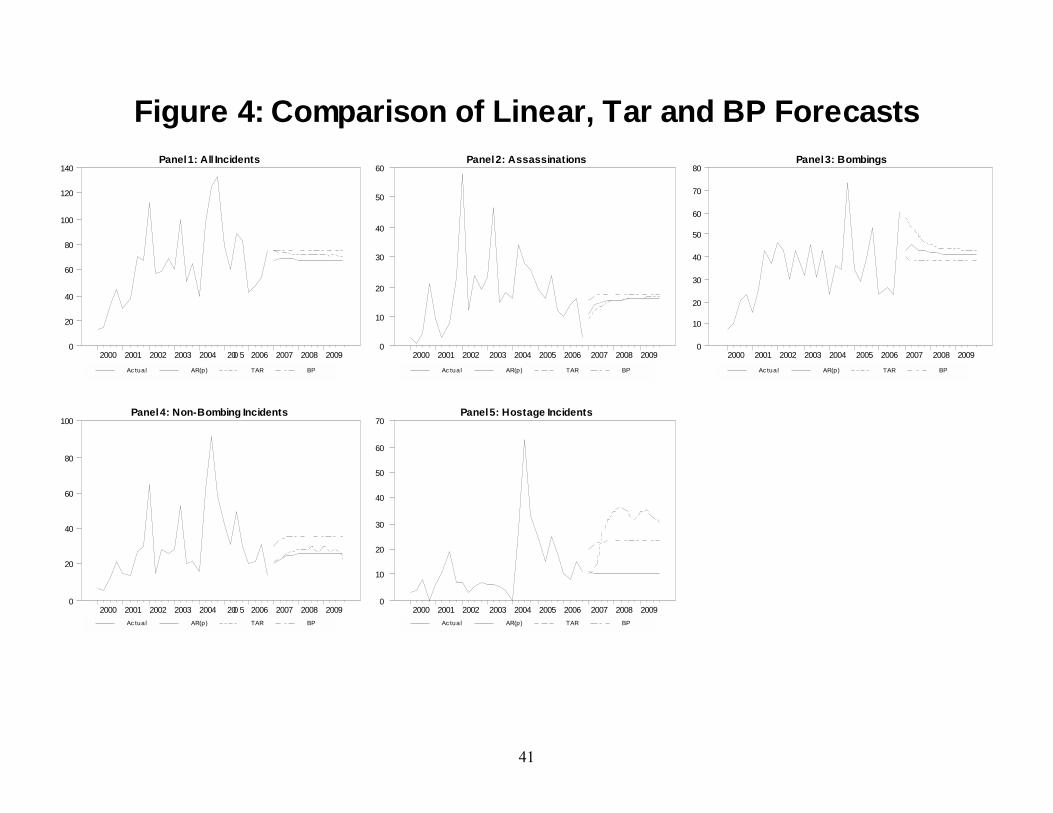
The comparison of the forecasts of the AR(p), TAR and BP is shown in Figure 4. The

TAR and AR(p) models have similar forecasts for all of the series except Hostage Incidents.

Since the AP model allows for no more than one break, it is not too surprising that the forecasts

from the AP and AR(p) models are similar. Since the BP model allows for up to four breaks, and

always selects a break sometime after 2001:1, it treats the latter data as a separate distinct period

from the earlier data. As such, the forecasts from the BP method are quite different from those of

the AR(p) and TAR models. For Total, Assassinations, Bombings, and Non-Bombings, the long-

run forecasts from BP are far greater than those of the other methods. The reason is that each

type of incident series rises in the latter part of the sample. For this reason, as can be seen from

Figure 5, the forecasts from BP are very similar to those using the �Known� break dates.

6. Conclusion

In this paper, we examine the problem of forecasting economic time-series with an

unknown number of structural breaks of unknown form. The in-sample and out-of-sample

properties of OS, NS and RS models are compared by using a Monte Carlo study with data

containing different degrees of persistence and different types of breaks.

When we pretend we do not know the true DGP of the experiment and apply the

competing models to estimate and forecast the data, some interesting results follow: First, the use

of the BIC to evaluate the in-sample performance of a model often overfits the data in that it

25

selects an overly complicated model in all of our experiments. Second, when the bias is used as

the out-of-sample evaluation criteria, there is no clear pattern which group of model consistently

forecast better when DGP is linear or TAR. The OS models (first differencing, exponential

smoothing and second differencing methods) outperform the NS and RS models when DGP

contains structural breaks. On the other hand, these methods very rarely minimize the MSPE.

Finally, when the MSPE is used as the out-of-sample evaluation criteria, we generally find that

OS models provide smaller MSPEs than their competitors when the DGP is linear or TAR. When

the DGP includes structural breaks, the NS models outperform the OS models only for cases

when the DGP has low persistence, relatively large structural breaks, and the breaks are not

offsetting.

A cursory check of the terrorism data indicates that the series do not seem to be highly

persistent. However, the wide variability across the various subsample periods and a brief review

of the modern-era terrorism history lead us to believe that the rise of religious fundamentalism,

the demise of the Soviet Union, and the rise of al Qaeda are likely to have caused changes in the

number of transnational terrorist incidents and in the nature of the incidents. Although it seems

reasonable to control for the number of breaks, the size of the breaks, and the form of the breaks,

NS models could not forecast as well as OS or RS models. The results suggest that the various

transnational terrorism series seem to either act as a TAR process or a linear process with

offsetting breaks. Since the forecasts from BP methods are very similar to those using the

�Known� break dates but different to those using OS models, the Monte Carlo exercise suggests

that we heavily discount the forecasts from the NS models in favor of those from the OS and RS

models.

26

In light of these conclusions, more effective policy responses can be devised to deal with

terrorism with different tactics by determining the �right� forecasting model. Besides, choosing

the model which provides better forecasting performance can assist policymakers in knowing

approximately how much to allocate to counterterrorist actions and the results might indicate

different terrorist attack level for US.

27

References

Andrews, Donald W. K. (1993), �Tests for Parameter Instability and Structural Change with Unknown Change Point,� Econometrica, 61, 821-856. Andrews, Donald W. K. and Werner Ploberger (1994), �Optimal Tests when a Nuisance Parameter is Present Only Under the Alternative,� Econometrica, 62, 1383-1414. Bai, Jushan and Pierre Perron (1998), �Estimating and Testing Linear Models with Multiple Structural Changes,� Econometrica, 66, 47-78. Bai, Jushan and Pierre Perron (2003), �Computation and Analysis of Multiple Structural Change Models,� Journal of Applied Econometrics, 18, 1-22. Clements, Michael and David Hendry, (1999), �Forecasting Non-stationary Economic Time Series,� The MIT Press: Cambridge, MA. Diebold, Francis and Lutz Kilian, (2000), �Unit Root Tests are Useful for Selecting Forecasting Models,� Journal of Business and Economics Statistics, 18, 265-273. Diebold, Francis X. and C. Chen (1996), "Testing Structural Stability with Endogeneous Break Point: A Size Comparison of Analytic and Bootstrap Procedures," Journal of Econometrics, 70, 221-241. Elliott, Graham (2005), �Forecasting When There is a Single Break,� working paper, UCSD. Enders, Walter (2004), Applied Econometric Time Series, 2nd ed., John Wiley and Sons: Hoboken, N.J. Enders, Walter and Clive Granger (1998), "Unit-Root Tests and Asymmetric Adjustment with an Example Using the Term Structure of Interest Rates," Journal of Business and Economic Statistics, 16, 304-11. Enders, Walter and Ruxandra Prodan (2007), �Forecasting Persistent Data with Possible Structural Breaks: Old School and New School Lessons Using OECD Unemployment Rates,� The Handbook of Forecasting in the Presence of Structural Change, Frontiers of Economics and Globalization, volume 4, Elsevier. forthcoming. Enders, Walter, and Todd Sandler (1999), �Transnational Terrorism in the Post-Cold War Era,� International Studies Quarterly, 43, 145−67. Enders, Walter and Todd Sandler (2000) �Is Transnational Terrorism Becoming More Threatening?� Journal of Conflict Resolution, 44, 307−32. Enders, Walter and Todd Sandler (2002), �Patterns of transnational terrorism, 1970-99: Alternative Time Series Estimates,� International Studies Quarterly, 46, 145−65.

28

Enders, Walter and Todd Sandler (2004), �Transnational Terrorism 1968 � 2000: Thresholds, Persistence and Forecasts,� Southern Economic Journal, 71, 467 � 483. Enders, Walter and Todd Sandler (2006), The Political Economy of Terrorism. Cambridge University Press: Cambridge, UK. Koop, Gary, M. Hashem Pesaran, and Simon Potter (1996), �Impulse Response Analysis in Nonlinear Multivariate Models,� Journal of Econometrics, 74, 119�147. Liu, Yamei and Walter Enders (2003), �Out-of-Sample Forecasts and Nonlinear Model Selection With an Example of the Term-Structure of Interest Rates.� Southern Economic Journal, 69, 520 � 540. Perron, Pierre and Timothy J Vogelsang (1992), "Nonstationarity and Level Shifts with an Application to Purchasing Power Parity," Journal of Business & Economic Statistics, American Statistical Association, vol. 10(3), pages 301-20, July. Pesaran, M. Hashem and Allan Timmermann (2004), �How Costly is to Ignore Breaks when Forecasting the Direction of a Time Series?� International Journal of Forecasting, 20, 411-424. Prodan, Ruxandra (2007), �Potential Pitfalls in Determining Multiple Structural Changes with an Application to Purchasing Power Parity,� Journal of Business and Economics Statistics, forthcoming. Rapoport, David C. (2004), �Modern Terror: The Four Waves,� in Audrey K. Cronin and James M. Ludes (eds.), Attacking Terrorism: Elements of a Grand Strategy. Georgetown University Press Washington, DC, 46-73.

29

Table 1: Date and Location of Breaks in the Generated Data

No Location of Break

Case 1 50 up

Case 2 100 up

Case 3 130 up

Case 4 50 up, 100 down

Case 5 100 up, 130 down

Case 6 50 up, 100 down, 130 up

Case 7 50 up*0.5, 100 down, 130 up*0.5

Case 8 50 up*0.5, 100 down*0.5, 130 up

Notes:

1. The eight cases correspond to various combinations of the break dates that are likely to exist in the terrorism

data.

2. The �up� and �down� in the table above indicate that we design an upward or downward structural break. The

�up*0.5� and �down*0.5� imply that the breaks are half as tall as the other breaks.

Table 2: Results for Linear Data Generating Process

Persistence =0.5 Persistence =0.9 1st 2nd 3rd 1st 2nd 3rd

BIC BP 665 BP-a 668 AP 669 BP 660 BP-a 666 Pre 667 1 Step Bias BP-p 0.00 BP 0.00 BP-a 0.01 Es 0.00 Tar 0.00 AP-p 0.00 4 Step Bias AP-p 0.00 AP 0.00 BP-a 0.01 BP-a 0.00 BP 0.03 AP-a 0.06 12 Step Bias AP-a 0.00 AP 0.01 AP-p 0.01 BP 0.00 Mtar 0.03 AP-a 0.04 1 Step MSQ Arp 1.00 Pre 1.00 Arma 1.01 AP-p 0.99 AP 0.99 Arma 1.00 4 Step MSQ Arp 1.00 Pre 1.00 Arma 1.00 Arma 1.00 Arp 1.00 AP-p 1.01 12 Step MSQ Arp 1.00 Pre 1.00 Arma 1.00 Arp 1.00 Arma 1.00 AP-p 1.09

Notes:

1. The DGP process is yt=α1yt-1+ εt with the persistence parameter α1 = 0.5 and 0.9.

2. �1st�, �2nd�, and �3rd� are the top three models selected among all candidates that provide the lowest BIC, Bias

and MSPE.

Table 3: Results for the Threshold Data-Generating Process

Standard Deviation = 1 Persistence1 = 0.3 Persistence1 = 0.5 Persistence1 = 0.5

Persistence2 = 0.7 Persistence2 = 0.7 Persistence2 = 0.9

1st 2nd 3rd 1st 2nd 3rd 1st 2nd 3rd

BIC BP 669 Tar 673 BP-a 674 BP 667 BP-a 673 Tar 673 BP 661 BP-a 666 Pre 668 1 Step Bias BP-a 0.03 AP-p 0.03 AP 0.03 AP-a 0.01 Tar 0.02 AP-p 0.02 Tar 0.02 BP-a 0.02 AP 0.03 4 Step Bias BP-a 0.01 AP-p 0.02 AP 0.02 AP-a 0.00 AP-p 0.02 AP 0.03 AP-a 0.01 AP 0.01 AP-p 0.01 12 Step Bias Tar 0.00 D1 0.01 Es 0.01 BP 0.00 D1 0.03 Es 0.03 Mtar 0.01 AP-a 0.02 Arp 0.03 1 Step MSPE Tar 0.96 Arp 1.00 Arma 1.00 Arp 1.00 Arma 1.00 AP-p 1.01 Arp 1.00 Arma 1.01 AP-p 1.01 4 Step MSPE Tar 0.99 Arp 1.00 Arma 1.00 Tar 0.99 Arp 1.00 Arma 1.00 Arp 1.00 Arma 1.00 AP-p 1.02 12 Step MSPE Arma 1.00 Arp 1.00 Pre 1.02 Arp 1.00 Arma 1.00 AP-p 1.04 Arp 1.00 Arma 1.00 Mtar 1.01

Standard Deviation = 2 Persistence1 = 0.3 Persistence1 = 0.5 Persistence1 = 0.5

Persistence2 = 0.7 Persistence2 = 0.7 Persistence2 = 0.9

1st 2nd 3rd 1st 2nd 3rd 1st 2nd 3rd

BIC BP 854 Tar 859 BP-a 859 BP 852 BP-a 857 AP 858 BP 849 BP-a 855 Pre 857 1 Step Bias Mtar 0.00 Tar 0.00 AP-p 0.01 Pre 0.04 Arma 0.04 Arp 0.04 D2 0.01 D1 0.01 AP-p 0.02 4 Step Bias AP-p 0.00 AP 0.01 Tar 0.01 BP 0.04 BP-p 0.04 D1 0.04 D1 0.02 Tar 0.03 AP-p 0.03 12 Step Bias Mtar 0.01 AP-p 0.03 AP 0.03 AP-a 0.00 AP-p 0.00 AP 0.00 Arp 0.00 Arma 0.01 Es 0.02 1 Step MSPE Arma 1.00 Arp 1.00 Pre 1.00 Pre 1.00 Arp 1.00 Arma 1.00 Arma 1.00 Arp 1.00 AP-p 1.02 4 Step MSPE Arma 1.00 Arp 1.00 Pre 1.00 Arp 1.00 Arma 1.00 Pre 1.00 Arp 1.00 Arma 1.00 AP-p 1.04 12 Step MSPE Arp 1.00 Arma 1.00 Pre 1.00 Arp 1.00 Arma 1.00 Pre 1.00 Arp 1.00 Arma 1.00 Mtar 1.03

Notes:

1. The TAR model is generated with the format: yt=α10+α11yt-1+εt, if yt-1 >τ, and yt=α20+α21yt-1+εt, if yt-1 ≤τ. We report the results for the following

parameterizations: τ=0, α10=0.5, α20= −0.5 are used for all the experiments and α11, α21 are represented as persistence1 and persistence2 in the above table.

Table 4: Data Generated with Breaks-In Sample Results-Using BIC as Evaluation Criteria

Magnitude of Breaks = 1 std Smooth Break, Persistence = 0.5 Smooth Break, Persistence = 0.9 1st 2nd 3rd 1st 2nd 3rd

1 BP 665 AP 671 BP-a 671 BP 660 BP-a 666 Pre 667 2 BP 666 AP 669 BP-a 671 BP 659 BP-a 665 Pre 667 3 BP 666 AP 670 BP-a 670 BP 659 BP-a 664 Pre 666 4 BP 665 BP-a 670 AP 671 BP 660 BP-a 666 Pre 668 5 BP 666 AP 670 BP-a 670 BP 660 BP-a 666 Pre 667 6 BP 666 BP-a 670 AP 671 BP 660 BP-a 666 Pre 667 7 BP 666 BP-a 670 AP 670 BP 660 BP-a 666 Pre 668 8 BP 665 AP 669 BP-a 669 BP 661 BP-a 666 Pre 668

Magnitude of Breaks = 2 std Smooth Break, Persistence = 0.5 Smooth Break, Persistence = 0.9 1st 2nd 3rd 1st 2nd 3rd

1 BP 666 AP 672 BP-a 673 BP 661 BP-a 666 Pre 668 2 BP 667 AP 670 BP-a 674 BP 659 BP-a 665 Pre 667 3 BP 665 AP 669 BP-a 671 BP 659 BP-a 665 Pre 667 4 BP 666 BP-a 674 AP 677 BP 660 BP-a 665 Pre 667 5 BP 665 AP 670 BP-a 671 BP 660 BP-a 665 Pre 667 6 BP 667 AP 673 BP-a 673 BP 661 BP-a 666 Pre 668 7 BP 665 BP-a 671 AP 671 BP 659 BP-a 665 Pre 667 8 BP 665 AP 670 BP-a 670 BP 661 BP-a 666 Pre 668

Notes:

1. In the first column, numbers from 1 to 8 indicate the locations of structural breaks showed in Table 1.

2. To save space, we only present the results from smooth breaks. The results from sharp breaks are similar and

are available upon request.

Table 5: Data Generated with Smooth Breaks-Out of Sample Results-Bias

Magnitude of Breaks = 1 std Smooth Break, Persistence = 0.5 Smooth Break, Persistence = 0.9

Step 1st 2nd 3rd 1st 2nd 3rd

1 12 BP-p 0.02 BP 0.02 Es 0.05 BP-a 0.02 Es 0.03 D1 0.04 2 12 Es 0.03 BP 0.03 D1 0.03 AP-a 0.02 Pre 0.03 BP-p 0.04 3 12 D2 0.03 D1 0.22 Es 0.23 Tar 0.10 D1 0.15 BP-p 0.15 4 12 Es 0.00 Tar 0.01 BP 0.02 Pre 0.05 BP-a 0.08 AP 0.09 5 12 Tar 0.05 Arp 0.11 Pre 0.11 Tar 0.03 D1 0.05 Es 0.05 6 12 D2 0.11 Es 0.18 D1 0.18 Es 0.11 D1 0.12 Pre 0.19 7 12 BP-a 0.01 Es 0.03 D1 0.04 Pre 0.05 BP 0.05 D1 0.06 8 12 D1 0.06 Es 0.10 BP 0.25 BP-a 0.10 Es 0.13 D1 0.13



1 12 AP 0.01 D1 0.02 BP-p 0.02 BP-p 0.04 D1 0.06 Pre 0.06 2 12 Es 0.02 D2 0.02 D1 0.03 BP 0.04 D1 0.06 Es 0.06 3 12 D2 0.25 D1 0.29 Es 0.30 Es 0.08 D1 0.10 BP-p 0.34 4 12 D1 0.00 Es 0.01 BP 0.03 D2 0.06 Es 0.09 D1 0.09 5 12 D2 0.12 Tar 0.26 Arp 0.33 Tar 0.19 Es 0.20 Mtar 0.21 6 12 D2 0.05 D1 0.38 Es 0.38 Es 0.20 D1 0.21 Pre 0.32 7 12 AP-a 0.00 AP-p 0.03 AP 0.04 D1 0.02 BP-a 0.03 Es 0.04 8 12 D2 0.15 D1 0.25 Es 0.26 D2 0.05 Es 0.22 D1 0.23

Notes:

1. To save space, we only presented the results from smooth breaks and the forecasting results of step 12.

33

Table 6: The Frequency that Each Model is Selected as the Top 3 Performer

Using Bias as Out of Sample Forecasting Criteria Total by Model 1 std 2 std Low High Smooth Sharp

Arp 1% 1% 1% 1% 1% 1% 1% D1 23% 23% 23% 25% 21% 23% 23% D2 15% 13% 18% 18% 12% 15% 15% Pre 4% 5% 3% 0% 8% 5% 3% Es 22% 21% 24% 24% 20% 23% 22% Arma 1% 0% 1% 1% 1% 1% 1% AP 4% 5% 3% 4% 4% 5% 3% AP-p 3% 3% 3% 3% 3% 3% 3% AP-a 3% 3% 2% 2% 3% 2% 4% BP 9% 11% 7% 10% 9% 8% 11% BP-p 6% 6% 7% 5% 8% 5% 8% BP-a 5% 6% 3% 3% 6% 6% 3% Tar 3% 3% 2% 2% 4% 3% 2% Mtar 1% 0% 1% 0% 1% 1% 1% Total 100% 100% 100% 100% 100% 100% 100%

Notes:

1. �Total by Model� shows us the probability of a competing model been selected as the top 3 forecasters in all of

our Monte Carlo experiments. �1 std� and �2 std� means different standard deviation, �Low� and �High� means

the data generating persistence, and �Smooth� and �Sharp� means the type of the breaks in our experiments.

34

Table 7: Data Generated with Smooth Breaks-Out of Sample Results-MSPE



1 12 AP-p 1.00 AP 1.00 Arp 1.00 Arma 1.00 Arp 1.00 AP-p 1.06 2 12 BP 0.94 AP-p 0.95 AP 0.96 Arp 1.00 Arma 1.01 Mtar 1.10 3 12 BP 0.90 BP-p 0.91 AP-p 0.96 Arp 1.00 Arma 1.00 AP-p 1.12 4 12 Arp 1.00 Pre 1.00 Arma 1.00 Arma 1.00 Arp 1.00 AP-p 1.06 5 12 Arma 1.00 Arp 1.00 Pre 1.00 Arp 1.00 Arma 1.00 AP-p 1.12 6 12 Arma 1.00 Arp 1.00 Pre 1.00 Arma 1.00 Arp 1.00 Mtar 1.09 7 12 Arp 1.00 Pre 1.00 Arma 1.00 Arma 0.99 Arp 1.00 Mtar 1.04 8 12 Arma 1.00 Arp 1.00 Pre 1.00 Arp 1.00 Arma 1.01 Mtar 1.03



1 12 AP-p 0.89 AP 0.89 Arp 1.00 Arma 1.00 Arp 1.00 Mtar 1.08 2 12 AP 0.53 AP-p 0.53 BP 0.58 Arp 1.00 Arma 1.00 AP-p 1.05 3 12 BP 0.53 BP-p 0.54 Es 0.58 Arp 1.00 Arma 1.00 Mtar 1.04 4 12 BP 0.91 BP-p 0.97 Arma 0.99 Arp 1.00 Arma 1.00 AP-p 1.10 5 12 Pre 1.00 Arp 1.00 Arma 1.01 Arp 1.00 Arma 1.00 AP-p 1.10 6 12 AP 0.89 AP-p 0.90 BP 0.93 Arp 1.00 Arma 1.00 AP-p 1.10 7 12 Arp 1.00 Pre 1.00 Arma 1.01 Arma 1.00 Arp 1.00 AP-p 1.08 8 12 BP 0.76 Es 0.81 D1 0.85 Arma 1.00 Arp 1.00 Mtar 1.01

35

Table 8: The Frequency that Each Model is Selected as the Top 3 Performers

Using MSPE as Out of Sample Forecasting Criteria Total by Model 1 std 2 std Low High Smooth Sharp

Arp 25% 28% 21% 17% 33% 26% 24% D1 2% 0% 4% 1% 3% 2% 2% D2 0% 0% 0% 0% 0% 0% 0% Pre 8% 10% 6% 14% 1% 9% 7% Es 2% 1% 4% 4% 1% 2% 3% Arma 23% 26% 21% 14% 33% 24% 23% AP 6% 4% 7% 10% 1% 6% 5% AP-p 15% 15% 16% 10% 20% 14% 17% AP-a 2% 2% 2% 3% 1% 2% 2% BP 6% 4% 9% 13% 0% 7% 6% BP-p 5% 4% 7% 11% 0% 4% 7% BP-a 0% 0% 0% 0% 0% 0% 0% Tar 1% 1% 1% 1% 0% 1% 1% Mtar 3% 5% 2% 1% 6% 4% 3% Total 100% 100% 100% 100% 100% 100% 100%

Table 9: Persistence across Various Sample Periods

First-order Autocorrelation Coefficient

All 1968:2 to 1979:4 1980:1 to 1991:3 1991:4 to 2001:2 2001:2 to 2006:4 DF Test (t-stat)

All Incidents 0.53 0.53 0.13 0.50 0.27 -4.87

Assassinations 0.44 0.29 0.16 0.65 -0.02 -5.36

Bombings 0.42 0.45 0.03 0.15 -0.21 -5.18

Non-Bombings 0.56 0.36 0.32 0.74 0.29 -5.03

Hostage 0.52 0.13 0.37 0.42 0.58 -5.89

36

Table 10: Results for Transnational Terrorism Data

1st 2nd 3rd Total

BIC BP 1507 Mtar 1515 Arma 1522 1 Step Bias D2 6.65 BP-a 15.85 D1 21.72 4 Step Bias D1 59.45 BP 61.53 Mtar 64.30 12 Step Bias BP 3.52 Tar 4.98 Mtar 6.36 1 Step MSQ D2 0.08 BP-a 0.47 D1 0.89 4 Step MSQ D1 0.77 BP 0.83 Mtar 0.90 12 Step MSQ BP 0.17 Tar 0.33 Mtar 0.54

Assassinations BIC BP 1229 BP-a 1234 Tar 1239 1 Step Bias AR 0.60 Pre 0.60 Tar 0.94 4 Step Bias BP-a 0.11 BP 0.61 BP-p 1.43 12 Step Bias D2 5.68 AR 12.72 Pre 12.72 1 Step MSQ AR 1.00 Pre 1.00 Tar 2.46 4 Step MSQ BP-a 0.00 BP 0.00 BP-p 0.02 12 Step MSQ D2 0.20 AR 1.00 Pre 1.00

Bombing BIC BP 1438 BP-a 1445 Mtar 1449 1 Step Bias BP-a 7.68 BP 8.55 BP-p 8.55 4 Step Bias Mtar 28.26 Tar 32.56 AR 33.15 12 Step Bias Mtar 17.44 Tar 17.75 AR 19.99 1 Step MSQ BP-a 0.22 BP 0.28 BP-p 0.28 4 Step MSQ Mtar 0.73 Tar 0.96 AR 1.00 12 Step MSQ Mtar 0.76 Tar 0.79 AR 1.00

Non-Bombing BIC BP 1272 Tar 1278 Mtar 1279 1 Step Bias D2 1.94 AR 6.82 Pre 6.82 4 Step Bias BP 27.27 BP-p 29.20 Es 29.22 12 Step Bias AR 11.31 Pre 11.31 AP 11.31 1 Step MSQ D2 0.08 AR 1.00 Pre 1.00 4 Step MSQ BP 0.62 BP-p 0.72 Es 0.72 12 Step MSQ AR 1.00 Pre 1.00 AP 1.00

Hostage BIC BP 1064 Tar 1069 Arma 1071 1 Step Bias D2 4.59 D1 4.98 BP 5.43 4 Step Bias Tar 24.14 AR 24.30 Pre 24.30 12 Step Bias Tar 1.39 Mtar 1.41 AR 1.51 1 Step MSQ D2 0.44 D1 0.52 BP 0.61 4 Step MSQ Tar 0.99 AR 1.00 Pre 1.00 12 Step MSQ Tar 0.84 Mtar 0.87 AR 1.00

37

Table 11: Breaks and Break Dates Selected by the New School Methods

Variable Method Breaks Break Dates All Incidents AP-const

AP-pure BP-const BP-pure

1 1 4 2

1991:1 1991:1 1981:2, 1991:1, 1997:1, 2001:2 1981:2, 1991:1

Assassinations AP-const AP-pure BP-const BP-pure

1 1 4 4

1975:3 2001:3 1975:3, 1992:1, 1994:3, 2001:3 1975:3, 1992:1, 1994:3, 2001:3

Bombings AP-const AP-pure BP-const BP-pure

1 1 2 2

1991:1 1991:1 1981:2, 1991:1 1981:2, 1991:1

Non-Bombings AP-const AP-pure BP-const BP-pure

1 1 4 1

1975:3 2001:4 1975:3, 1983:4, 1996:4, 2001:2 1975:3,

Hostage AP-const AP-pure BP-const BP-pure

1 1 3 0

1999:1 1984:2 1984:2, 1987:1, 1999:1

Figure 1: The Five Terrorism SeriesTotal

1968 1971 1974 1977 1980 1983 1986 1989 1992 1995 1998 2001 20040

25

50

75

100

125

150

175

200

225

BOMBINGS NON_BOMB

Bombings and Non-Bombings

1968 1971 1974 1977 1980 1983 1986 1989 1992 1995 1998 2001 20040

25

50

75

100

125

150

175

Assassinations

1968 1971 1974 1977 1980 1983 1986 1989 1992 1995 1998 2001 20040

10

20

30

40

50

60

Hostage Takings

1968 1971 1974 1977 1980 1983 1986 1989 1992 1995 1998 2001 20040

10

20

30

40

50

60

70

39

Figure 2: The Eight BreaksCase 1

20 40 60 80 100 120 1400.000.250.500.751.001.251.501.752.00

Case 2

20 40 60 80 100 120 1400.000.250.500.751.001.251.501.752.00

Case 3

20 40 60 80 100 120 1400.000.250.500.751.001.251.501.752.00

Case 4

20 40 60 80 100 120 1400.000.250.500.751.001.251.501.752.00

Case 5

20 40 60 80 100 120 1400.000.250.500.751.001.251.501.752.00

Case 6

20 40 60 80 100 120 1400.000.250.500.751.001.251.501.752.00

Case 7

20 40 60 80 100 120 1400.000.250.500.751.001.251.501.752.00

Case 8

20 40 60 80 100 120 1400.000.250.500.751.001.251.501.752.00

40

Figure 3: Comparison of the Old School Forecasts

Ac tual AR(p) D1 Es

Panel 1: All Incidents

2000 2001 2002 2003 2004 200 5 2006 2007 2008 20090

20

40

60

80

100

120

140

Ac tual AR(p) D1 Es

Panel 4: Non-Bombing Incidents

2000 2001 2002 2003 2004 200 5 2006 2007 2008 20090

20

40

60

80

100

Ac tual AR(p) D1 Es

Panel 2: Assassinations

2000 2001 2002 2003 2004 2005 2006 2007 2008 20090

10

20

30

40

50

60

Ac tual AR(p) D1 Es

Panel 5: Hostage Incidents

2000 2001 2002 2003 2004 2005 2006 2007 2008 20090

10

20

30

40

50

60

70

Ac tual AR(p) D1 Es

Panel 3: Bombings

2000 2001 2002 2003 2004 2005 2006 2007 2008 20090

10

20

30

40

50

60

70

80

41

Figure 4: Comparison of Linear, Tar and BP Forecasts

Ac tual AR(p) TAR BP


2000 2001 2002 2003 2004 200 5 2006 2007 2008 20090

20

40

60

80

100

120

140



2000 2001 2002 2003 2004 200 5 2006 2007 2008 20090

20

40

60

80

100



2000 2001 2002 2003 2004 2005 2006 2007 2008 20090

10

20

30

40

50

60



2000 2001 2002 2003 2004 2005 2006 2007 2008 20090

10

20

30

40

50

60

70


Panel 3: Bombings

2000 2001 2002 2003 2004 2005 2006 2007 2008 20090

10

20

30

40

50

60

70

80

42

Figure 5: Comparison of Linear, 'Known' and BP Forecasts

Actual AR(p) 'Known' BP


2000 2001 2002 2003 2004 2005 2006 2007 2008 20090

20

40

60

80

100

120

140



2000 2001 2002 2003 2004 2005 2006 2007 2008 20090

20

40

60

80

100

Ac tual AR(p) ' Known' BP


2000 2001 2002 2003 2004 2005 2006 2007 2008 20090

10

20

30

40

50

60

Ac tual AR(p) ' Known' BP


2000 2001 2002 2003 2004 2005 2006 2007 2008 20090

10

20

30

40

50

60

70


Panel 3: Bombings

2000 2001 2002 2003 2004 2005 2006 2007 2008 20090

10

20

30

40

50

60

70

80

Forecasting Series Containing Offsetting Breaks: Old...

Documents

Transcript of Forecasting Series Containing Offsetting Breaks: Old...