Forecasting Methods

Mark Little, SAS Institute Inc., Cary NC

ABSTRACT

This paper is a tutorial on time series forecasting methods. It pro­vides a brief survey of time series forecasting tools in the SAS Sys­

tem, principally in SAS/ETS® software.

INTRODUCTION

There are many things you might want to forecast. This paper dis­cusses time series forecasting. By time series forecasting we mean that you have something that is measured regularly over time and want to predict the value at future time periods.

An example is forecasting the monthly sales of some product. An­other example is forecasting gross national product measured quarterly.

Time series forecasting methods include judgmental methods, structural models, and time series methods.

Judgmental methods make use of personal opinions and judge­ments. The problems with judgmental methods are subjectivity and poor accuracy in practice.

Structural models use independent variables to predict dependent variables. For example, you might use projected population growth to forecast the demand for new housing. Using independent vari­ables in forecasting models requires forecasts of the independent variables. In order to use structural models for forecasting, you also need to know how to forecast time senes without using independent variables.

Time series methods use mathematical models or procedures-that extrapolate predicted future values from the known past of the se­ries.

The topic of this paper is forecasting time series of numbers mea­sured periodically (for example, monthly or quarterly) based on mathematical procedures applied"to the known history of the series.

SAS/ETS software provides many forecasting methods. To use these' methods, you can either enter SAS statements for SAS/ETS procedures, or you can use the new interactive forecasting ,menu system. The menu system generates all necessary SAS state­ments through a graphical user interface, which makes it very easy to do time series forecasting.

411

This tutorial paper focuses on SAS/ETS procedures and gives little attention to the forecasting menu system. However, keep in mind that there is an easier way to use these methods.

Time series forecasting methods often are based on statistical time series models. You fit a statistical model to the time series process and then use the model to generate forecasts.

This paper considers time series models as heuristic tools for cap­turing and extrapolating patterns in the data. The kinds of patterns of interest are trend, autocorrelation, seasonality, and interven­tions.

FORECASTING TREND

To begin, consider the problem of forecasting trend. (Interventions and forecasting seasonality and short run autocorrelation patterns are discussed later.)

If you want to extrapolate past trends, the first thing you have to do is decide what you mean by trend.

For example, here is a plot of the U.S" unemployment rate for 1980 through 1991. Suppose it was still early 1992 and you wanted to forecast the unemployment rate based on the trend in this data.

LHUR 12 10 8

6

U.S.~RaIe

4 "-r-,-.-,-,,-r-.-.-.-,--.-,

8 8 8 8 8 8 8 8 8 8 9 9 9 0123456789012

Dale of Observalion

What is the trend in this series? This series has a trend, but the trend changes depending on what part or how much of the data you look at.

Time Trend Regression

Unear regression is widely used for forecasting, and regression on time is an obvious way of extrapolating a trend. So begin by fitting a constant time trend to the unemployment series by. linear regres­sion.

Use the DATA step to create mo time variables. The first time in­dex T counts observations. The second index is the same, but has missing values for years before 1989.

data a; set ai t + 1. if date >= 'lj-an89'd then t89 t; else t89 .;

run;

Next run PROC REG mice, regressing the unemployment rate first on time for the whole period and then on time only for observations since 1989. Output the predicted values from the two regressions and merge the data sets.

proc reg data=a; model lhur = t; output out=bl p=p;

run;

proc reg data=a; model lhur = t89; output out=b2 p=p89;

run;

data bi merge bl b2; by date;

run;

Then make an overlay plot of the predictions from the two regres­sions using PROC GPLOT. The following GPLOT statements are needed.

proc gplot data=b; plot lhur*date=l p*date=2 p89*date=3

overlay hax!s='ljan80'd to 'ljan94'd

by year; symboll v=plus i=join; symbo12 v=none i=join; symbol3 v=ncne i=join; format date year2.;

runi

These statements produce the following plot.

412

lHUR 12

10

B 6

4

Trne Trends Fit by Li1ear Regn.ssio.l

B B B 0 1 2

B 3

B B B B B B 9 999 9 4 5 6 7 B 9 0 1 234

Dale of OOOeNalOO

Clearly, you get very different forecasts depending on what part of the data you look at. Which trend line is more appropriate depends on whether you are interested in short term or long term forecasts. This plot teaches two important lessons.

First, the choice of a forecasting method depends on how far you want to forecast. Time series have short run trends within long-run trends. For short-term forecasts, you want to look at recent move­ments. For long-term forecasts, you want to look at the larger pat­tern and discount the short run fluctuations.

Second, time-trend regression, while very simple, is often not a very good forecasting technique. Any fixed trend line is usually too in­flexible to capture the patterns in the data and does not discount the past appropriately. Good forecasting methods can tracka smoothly changing trend, and they give more' weight to the recent past than to the more distant past.

Exponential Smoothing

Exponential smoothing is a very simple method that discounts the past with exponentially declining weights. The smoothe,d values are moving averages of past values, with the weights of the moving average declining exponentially with distance into the past.

The degree of smoothing is controlled by a smoothing weight. Smaller smoothing weights discount the past less and can pick up longer run trends. Larger weights track the data more closely and forecast the short run trend.

Exponential smoothing is a very popular forecasting method, partly because it is so simple and partly because it seems to work quite well in practice ..

Single exponential smoothing is just a weighted average of the past value where the weights are an exponential function of how far into the past the value is. Single exponential smoothing is useful when you know there is no trend and the series fluctuates about a fixed mean. The forecasts from single exponential smoothing are con­stant.

Double exponential smoothing applies single exponential smooth­ing twice and so produces an exponentially smoothed trend. The forecasts from double exponential smoothing follow a straight line trend.

Triple exponential smoothing produces an exponentially smoothed change in trend. The forecasts from triple exponential smoothing follow a quadratic trend.

The FORECAST procedure in SAS/ETS software performs expo­nential smoothing. The INTERVAL=MONTH option tells the proce-

dure thaI the data are monthly, and the LEAD=24 option specifies forecasting 24 months past the end of the data.

The METHOD. option combined with the TREND-2 option speci­fies double exponential smoothing. The WEIGHT = option specifies the smoothing weight as .15. The output options include both the forecasts and the historical data and within·sample predicted val· ues in the output data set.

proc forecast data=a out=b lnterval=month lead=24 method=expo trena=2 welgbt=.lS outpredlct outlstep outactual;

id date; var Ihur;

run;

After producing the double exponential smoothing forecast with PROC FORECAST, use PROC GPLOT 10 pial the forecasts. The FORECAST procedure stores actual and predicted values under the original variable name and uses the _TYPE_ variable to distin· guish the different kinds of observations. Thus you use the _ TYPE_ variable in the PLOT statement to separate the values into separate actual and predicted plots.

proc gplot data=b &gout; plot lhur-date=_type_

hax1s='1janSO'd to Iljan94 1 d by year;

symbol1 v=plus l=join w=4; symbo12 v=none l=joln w=4; format date year2. j

run;

Following is the plot of the exponential smoothing results. Notice that the forecast produced by double exponential smoothing is a straight line, just as for linear time trend regression.

Double ExpmenIiaI Sm:x:lIhi'll WEIGH!" = .15

LJ-lUR 12

10

8

6

4

8 8 8 8 8 8 8 8 8 8 9 9 9 9 9 0 1 2 3 4 5 6 7 8 9 0 1 2 3 4

Dale of 0bseMIIiJn

A key problem with exponential smoothing is how to choose the smoothing weight Different smoothing weights produce a different compromise between the short run and long run trends in the data, and thus produce different forecasts.

How to choose an appropriate smoothing weight is a complex ques­tion. It depends on the intended forecast horizon; that is, on whether you are interested in short or long term forecasts. It de­pends on the volatility of the series; more volatile series need more smoothing since recent values contain more noise and less infor­mation about local trend. It depends on how strongly you believe that the series has a stable long run trend.

A popular approach is to find an 'optimal" weight that minimizes the

413

within sample mean square one-step prediction error. However, such a weight is only optimal if you really believe that exponential smoothing is the correct model for the data.

Another problem with exponential smoothing is how to set the start­ing values for the smoothing equations. Various different methods of computing starting values have been proposed, but they are all very ad hoc. PROC FORECAST provides options to control start­ing values and supports all the usual methods. For long series and little smoothing, starting values don't matter; but for short series or small smoothing weights, this issue can make a big difference to the forecasts.

Exponential smoothing is mathematically equivalent to a particular ARIMA model, and if you believe this model you can use PROC ARIMA to fit and forecast the exponential smoothing model in a sta­tisti~ly optimal way. The ARIMA model correctly handles both es­timation of the weights and the starting values problem.

In practice you don't usually think that exponential smoothing is a model for the series; instead, exponential smoothing is used as a convenient way of smoothing trend and discounting the past.

Forecasting with ARIMA Models

A more statistically sophisticated approach to forecasting is the ARIMA model or Box-Jenkins method. ARIMA modeling is a com­plex subject, and this paper can give only a very superficial intro­duction of the ideas as they relate to forecasting.

The ARIMA method combines three ideas. First, in ARIMA model­ing you account for trend by differencing the series. Instead of modeling and forecasting the series itself, you forecast the period­to-period changes in the series, and then add up-or integrate­the predicted changes to get the final forecast. This idea of inte­grating predicted changes is where the "" in ARIMA comes from.

The second idea in ARIMA modeling is predicting the series by lin­ear combination of its recent past values. Since you in effect regress the series on its I~gged values, this is called autoregres­sion. This is where the "AR~ in ARIMA comes from.

The third idea in ARlMA modeling is to take weighted moving aver­ages of past errors. The use of moving average error processes is where the "MA" in ARIMA comes tram.

The class ofARIMA models is very general and encompasses many simpler forecasting methods as special cases. For example, you have already seen a moving average model in the case of ex­ponential smoothing. Double exponential smoothing is equivalent to a restricted second-order moving average process applied to the second difference of the series. 'with the moving average parame­ters determined by the exponential smoothing weight and with the intercept term omitted.

You can combine regression inputs with ARIMAmodels, and so re­gression methods can also be seen as a special case of ARIMA model forecasting. The ARIMA procedure is used to forecast with ARIMA models.

The following example uses a first-order autoregressive model for the Changes of the unemployment series. The IDENTIFY state­ment specifies the unemployment rate variable as the series to ana­lyze and specifies first differencing the series. The ESTIMATE statement fits a first-order autoregressive model to the differenced series~the p= option gives the autoregressive order. This is called an ARIMA(1, 1.0) model. since there is 1 autoregressive lag, the series is differenced once, and there is no moving average part. The forecast statement creates ·the output data set and produces

forecasts from the model for 24 months past the end of the data.

proc arima data=a; identify var=lhur(l); estimate p=l; forecast out=b id--date

interval=mcnth lead=24; runi

The following GPLOT statements plot the ARIMA model results. The ARIMA procedure stores the predicted values in the variable FORECAST

proc gplot data=b; plot lhurwdate=l forecast-date=2 I

overlay href='15dec90'd chref=green haxis='ljan80'd to '!jan94'd by year

symbol! v=plus i=join w=4; symbo12 v=none i=join w=4 c=eyan; for.mat date year2.i

run;

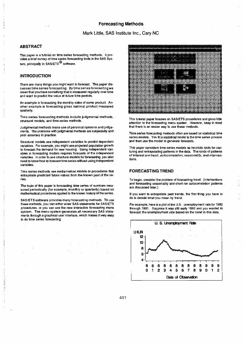
The following is the plot of the ARIMA(l ,.1 ,0) model predictions.

U;UR 12 10 B

6

4

B B. 0 1

8 2

ARIMA(1,l,O) Model

B 3

B B B 8 B 8 9 9 9 9 9 4 5 6 7 B 901 234

Dale of 0bservatiJn

The"long run forecasts from an ARIMA model with first-order differ­encing is a straight line, with the slope determined by the intercept term of the model. That is, the slope depends tin the average differ­ence over the period of fit. For second-order differencing, the long­run forecast is a quadratic trend.

The short run forecast from the ARIMA model incorporates recent departures from trend. The effect of the autoregressive part of the model declines exponentially to zero as the forecast horizon in­creases. The effect of the moving average part falls to zero once the forecast horizon extends beyond the order of the moving aver­age model.

Thus-the ARIMA model produces a compromise between short run forecasts from an autoregressive moving average model for recent patterns in the data ana Ibng run forecasts based on the average rate of change in the series.

Time Trend Regression with Autoregressive Errors

Differencing the series and modeling the period-to-period changes is a more flexible way to handle long run trend than using a fixed time regression. Differencing-allows a stochastic trend. while time regression assumes a deterministic trend.

414

However, if you want to assume a deterministic global trend, you can combine time trend regression, as you saw in the first forecast­ing example using PROC REG, with an autoregressive model for departures from trend.

You can fit and forecast a time trend with an autoregressive error model using PROC ARIMA by specifying a time index as an input variable. Or you can regress the dependent variable on time with PROC AUTOREG. However, the simplest way to forecast with this model is to use PROC FORECAST.

The PROC FORECAST statements for this method are similar to those used for exponential smoothing, except that you specify the STEPAR method. The STEPAR method regresses the series on time and then selects an autoregressive model for the residuals us­ing a stepwise technique.

proc forecast data=a out=b

id date; var Ibur;

run;

metbod=stepar trend=2 Interval=montb lead=24 outpredict outlstep outactual;

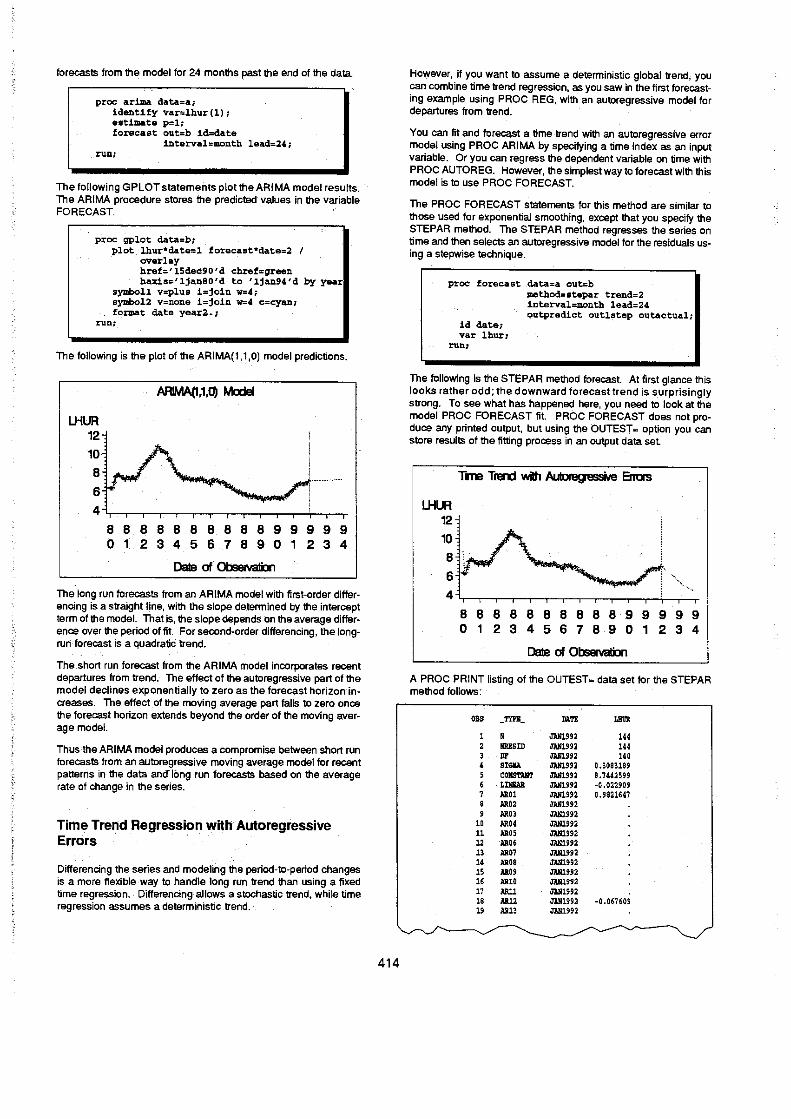
The following is the STEPAR method forecast. At first glance this looks rather odd; the downward forecast trend is surprisingly strong. To see what has happened here, you need to look at the model PROC FORECAST fit. PROC FORECAST does not pro­duce any printed output, but using the OUTEST:: option you can store results of the fitting process in an output data set

U;UR 12

1~~ 6

4~~'-"-'-''-.-,,-.~-r~ B B B B 8 8 8 B B B 9 9 9 9 9 o 1 2 3 4 5 6 7 890 1 234

Dale of Observalbn

A PROC PRINT listing of the OUTEST = data set for the STEPAR method follows:

O.S _TYPE_ DATE La"" , JANl992 '44 2 ""SID JANl992 '44 3 Dl' J1Nl.992 '40 • "GIlA JANl992 0.3083189 5 COIlS'l'All'r JANl992 8.7"2599 , LINIAR JANl992 -0.022909 1 lR01 JlN1992 0.9821647 8 AR02 JANl992 , AR03 JAN1992

10 .. " JANl992 11 .. 05 JAN1992 12 -Alt06 JAN1992

" .RD1 JAN1992 14 .RD8 JAN1992 15 AR" JANl992 16 ARlO JAN1992 11 AR11 JANl992 18 AR12 JANl992 -0.067609 19 AR" JAN1992

20 SS'r mUg2 297.44 21 SSB JANU9:! 10.69686 22 lIS! JANUS2 O~O76'O61

23 "'" JANl!!!!2 0.2764166

" WI JANl.992 2.:1406541

" !PI m1g!!:! ~O.O9683

" ... JlNl.992 0.1559265

" .. JlNl.992 0.0046451

" Jl,SQO'W J1Nl.992 0.96403"

This listiI!9 shows the coefficients of the time trend regression and the signific~J"t autoregressive parameters, as well as various de­scriptive statistics. There are 2 significant autoregressive ,parame­ters retained by the stepwise selection metho~, at lags 1. and 12.

The lag 1 :autoregressive parameter is .98. This means that the residuals about the fixed trend line are almost a random walk, and once the series departs from trend it will take a long time to return to trend. (This case can also be seen as an example of the limita­tion of time regression as compared with differencing as a means of 'detrending" data.)

You can better see what is going on here by extending the forecast horizon. If you run the forecast to the year 2000, the results look more reasonable. The prediction of the STEPAR method is that the, rate will return gradually to the long run trend line. You can see this even better by overlaying a plot of the time regression line, as in the following plot.

l.HUR 12 10 8 6 4

Tme Trend v.iIh AuIoregressille Errors

2~rr"""""~rT"-'''~ 888888888899999999990 012345678901234567890

Dale of 0bservaIi:Jn

Deterministic versus Stochastic Trend Models

If you want to assume a gl'obal deterministic trend, the STEPAR method-is a very good foreCasting method. However, the assump­tion of a fixed deterministic trend line is often very doubtful, and methods that handle trend by differences, such as exponential smoothing and other ARIMA models, may be preferable.

So far you have looked at two different approaches to forecasting trend. You can assume a deterministic trend or a stochastic trend. You can model deterministic trend with time regression; stochastic trend you can model by differencing the series.

You've looked at two methods for each approach. Fordeterministic trend you looked at simple time trend regression and time regres­sion plus an autoregressive error model, which is much better. For stochastic trend you looked at double exponential smoothing and an ARIMA(l, 1,0) model.

415

CHOOSING THE RIGHT FORECASTING METHOD

There are of course many other methods you could examine. But one thing that is ~ready clear is that different methods give different forecasts. Now turn to the issue of selecting from among available forecasting methods.

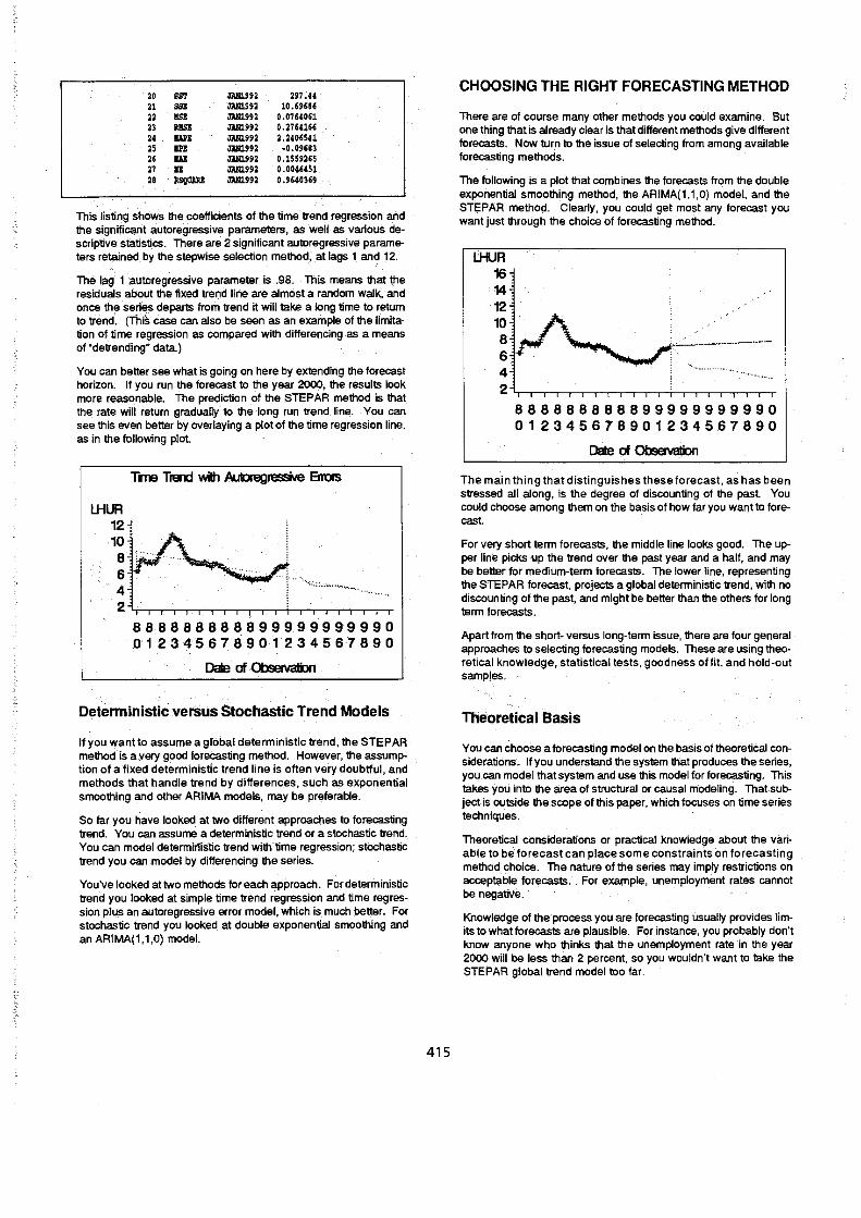
The following is a plot that combines the forecasts from the double exponential smoothing method, the ARIMA(l, 1,0) model, and the STI;PAR method. Clearly, you could get most any forecast you want just through the choice of forecasting method.

l.HUR 16 14 12 10 8 6

'~.-..•. -.-.-.. -.. -

4

2""-."-.,,-.,,~rr,,,,,,~ 888888888899999999990 012345678901234567890

Dale of 0bservatiJn

The main thing that distinguishes these forecast, as has been stressed all along, is the degree of discounting of the past. You could choose among them on the basis of how far you want to fore­cast.

For very short term forecasts, the middle line looks good. The up­per line picks ,up the trend over the past year and a half, and may be better for medium-term forecasts. The lower line, representing the STEPAR forecast, projects a global deterministic trend, with no discounting of the past, and might be better than the others for long term forecasts.

Apart from the short- versus long-term issue, there are four general approaches to selecting forecasting models. These are using theo­retical knowledge, statistical tests, goodness of fit, and hold-out samples.

Theoretical Basis

You can choose a forecasting model on the basis of theoretical con­siderations. If you understand ,the system that produces the series, you can model that system and use this model for forecasting. This takes you into the area of structural or causal modeling. That sub­ject is outside the scope of this paper, which focuses on time series techniques.

Theoretical considerations or practical knowledge about the vari­able to beforecast can place some constraints on forecasting method choice. The nature of the series may imply restrictions on acceptable forecasts. For example, unemployment rates cannot be negatiVe.

Knowledge of the process you are forecasting usually provides lim­its to what forecasts are plausible. For instance, you probably don't know anyone who thinks that the unemployment rate in the year 2000 will be less than 2 percent, so you wouldn't want to take the STEPAR global trend model too far.

Statistical Tests

In the statistical modeling approach to data analysis, you fit models to data and choose among possible models on the basis of statisti­cal diagnostics and tests. The Box-Jenkins method for developing ARIMA models is a good example of this approach for time series modeling.

Diagnostic checking usually includes significance of parameters, autocorrelation of residuals, and normality of residuals. Acceptable models can then be compared on the basis of goodness of fit and parsimony of parameterization.

The statistical modeling approach can be a very effective way to develop forecasting models. But there are several drawbacks.

The purpose of statistical modeling is to find an approximation to the data generating process producing the series. For forecasting you don't really care about that and are just interested in capturing and extrapolating patterns in the data.

Statistical model diagnostic tests are not directly related to how well the model forecasts. Moreover, statistical tests are based on the assumption that the model is a correct representation of the data generating process. In practice, forecasting models are usually 'wrong" in this sense, and statistical tests may not be valid.

Some forecasting competitions have found that models developed by the Box·Jenkins approach often performed worse than exponen· tial smoothing or other simpler methods. This suggests that statisti­cal modeling criteria may not produce the best forecasting method.

Goodness-ot-Fit Comparisons

One obvious and reasonable approach to forecasting method se-­lection is to choose the method that best fits the known data. You compare the forecasting methods considered using some measure of goodness of fit. This is usually based on one-step-ahead residu· als for the whole sample.

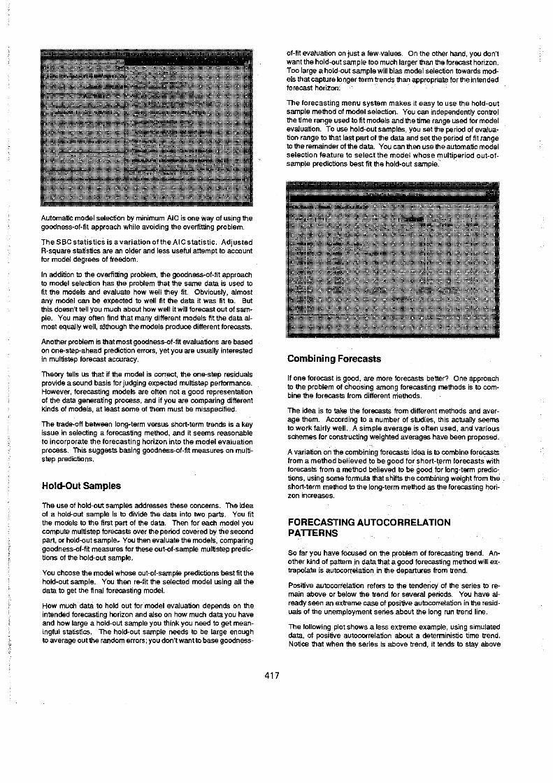
There are many different statistics available for measuring good­ness of fit. Following is the menu of choices provided by the fore-­casting menu system.

The most often used statistic is the mean square error. Other com· manly used measures are the mean absolute error and the mean absolute percent error. The forecasting menu system displays the selected statistics for a forecasting method as folloWs:

416

One advantage of the goodness-ot-fit approach to forecasting method selection is that once you have decided on the measure to use, the Whole process can be automated.

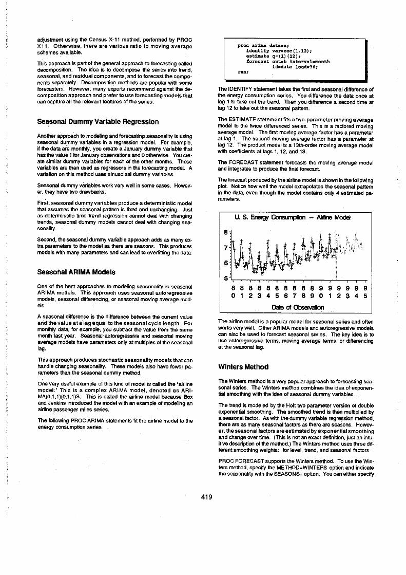
The forecasting menu system supports automatic forecasting in this way. You tell it which measure of goodness of fit you want to use as the selection criterion. You then select all the forecasting models you want to consider from-a list of available models. Once you've specified the list of models to try, the menu system fits all the candidate models and keeps the one that fits the data best.

The following is the menu for specifying the forecasting models to try. All the highlighted models will be fit, and the best fitting will be used for forecasting.

There are several problems with using goodness of fit as the basis for choosing forecasting methods. You can always get a better fit by going to a more complex model, but more complex models often perform worse for forecasting. You want the model to fit the data, but you want to avoid overfitting the data.

One way to guard against overfitling is to use statistical tests to throw out insignificant parameters. However, there are limitations to this approach, as discussed previously.

A more promising approach is to use criteria that trade off goodness of fit and model parsimony. Akaike's information criterion, b(AIC, is a goodness-ot-fit measure that penalizes for the number of pa­rameters in the forecasting model.

Automatic model selection by minimum AIC is one way of using the goodness-of-fit approach while avoiding the overfitting problem.

The5BC statistics is a variation of the Ale statistic. Adjusted R-square statistics are an older and less useful attempt to account for model degrees of freedom.

In addition to the overfitting problem, the goodness-of-fit approach to model selection has the problem that the same data is used to fit the models and evaluate how well they fit. Obviously, almost any model can be expected to well fit the data it was fit to. But this doesn't tell you much about how well it will forecast out of sam­ple. You may often find that many different models fit the data al­most equally well, although the models produce different forecasts.

Another problem is that most goodness-cf-fit evaluations are based on one-step-ahead prediction errors, yet you are usually interested in multistep forecast accuracy.

Theory tells us that if the model is correct, the one-step residuals provide a sound basis for judging expected multistep performance. However, forecasting models are often not a good representation of the data generating process, and if you are comparing different kinds of models, at least some of them must be misspecified.

The trade-oft between long-term versus short-term trends is a key issue in selecting a forecasting method, and it seems reasonable to incorporate the forecasting horizon into the model evaluation process. This suggests basing goodness-of-fit measures on multi­step predictions.

Hold-Out Samples

The use of hold-out samples addresses these concerns. The idea of a hold-out sample is to divide the data into two parts. You fit the models to the first part of the data. Then for each model you compute multistep forecasts over the period covered by the second part, or hold-out sample .. You then evaluate the models, comparing gOodness-of-fit measures for these out-of-sample multistep predic­tions of the hold-out sample.

You choose the model whose out-of-sample predictions best fit the hold-out sample. You then re-fit the selected model using all the data to get the final forecasting model.

How much data to hold out for model evaluation depends on the intended forecasting horizon and also on how much data you have and how large a hold-out sample you think you need to get mean­ingful statistics. The hold-out sample needs to be large enough to average out the random errors; you don't want to base goodness-

417

of-fit evaluation on just a few values. On the other hand, you don't want the hold-outsample too much larger than the forecast horizon. Too large a hold-out sample will bias model selection towards mod­els that capture longer term trends than appropriate for the intended forecast horizon. '

The forecasting menu system makes it easy to use the hold-out sample method of model selection. You can independently control the time range used to fit models and the time range used for model evaluation. To use hold-out samples, you set the period of evalua~ tion range to that last part of the data and set the period of fit range to the remainder of the data. You can then use the automatic model selection feature to select the model whose multiperiod out-of­sample predictions best fit the hold-out sample.

Combining Forecasts

If one forecast is good, are more forecasts better? One approach to the problem of choosing among forecasting methods is to com­bine the forecasts from different methods.

The idea is to take the forecasts from different methods and aver­age them. According t6 a number of studies, this actually seems to work fairly well. A simple average is often used, and various schemes for constructing weighted averages have been proposed.

A variation on the combining forecasts idea is to.combine forecasts from a method believed to be good for short-t,~rm forecasts with forecasts from a method beheved to be good tor long-term predic­tions, using some formula that shifts the combining weight from the short-term method to the long-term method as the forecasting hori­zon increases.

FORECASTING AUTOCORRELATION PATTERNS

50 far you have focused on the problem of forecasting trend. An­other kind of pattern in data that.a good forecasting method will ex­trapolate is autocorrelation in the departures from trend.

Positive autocorrelation refers to the tendency' of the series to re­main above or below the trend for several periods. You have al­ready seen an extreme case of positive autocorrelation in the resid­uals of the unemployment series about the long run trend line.

The following plot shows a less extreme example, using simulated data, of positive autocorrelation about a deterministic time trend. Notice that when the series is above trend, it tends to stay above

trend for several periods. Likewise, downward departures from trend also tend to persist.

Y <10

30

20

10

Tme Trend wiIh .Fa;iive AuIccoi, eBIb1

... ~ .... .- .......•.. ~ ~

... . .. "'~ .' ~"'"~'." ,

O~~~~~~~~~ __ -r~~-T ..

o 10

.

20

TIME

30 <10

Negative autocorrelation refers to "the tendency of the series to re­bound. from departures from trend, s,o that unexpectedly low values are followed by comperisating high·:YaJues in. the next period, and vice versa. The following" is a ptot of a simulated time series show­ing a deterministic time trend plus a negatively autocorrelated error.

Y <10

o

Tme Trend with Negalille AuIccoi,eIaIiA ,

10 20

mE 30 <10

When autocorrelation is present. you can use the deviations from trend at'the end of the series to improve the short run forecast For example, suppose the last data value is above the estimated trend. If the series has positive autocorrelation, you can predict that the next value will also be above trend. On the .other hand, if the senes has negative autocorrelation, you can predict that the next value will rebound below tr~nd.

Autoregressive models and ARIMA models are very good at this; indeed, thafs what they are designed for. On the other hand, re­gression methods and exponential smoothing methods do not mod­el autocorrelation ..

Autocorrelation pattern!i. in time series can be very complex. Au­toregressive models and ARIMA models can handle all kinds of au­tocorrelation patterns. The Box-Jenkins method of selecting ARI­MA models is based on examining the pattern of autocorrelations at different lags. Following is an example of how the forecasting menu system displays autocorrelation function plots.

418

FORECASTING SEASONALITY

One special and very important kind of autocorrelation is seasonali­ty. Many time series are regularly higher or lower at particular times oftheyear _ Forexample, sales of heating oil are usually much greater in the winter than in the summer.

You also use the term seasonality for any recurring cyclic pattern with a fixed period. For example, with daily data you often find that weekends are very different from weekdays. With hourly data, you usually find that values are consistently different for nighttime hours than for daylight hours.

The following is a plot of monthly U.S. energy consumption. Just looking at this plot, you can see both a Winter peak and a smaller summer peak. Clearly, to forecast this series you must take the seasonal pattern into account.

8 8 o 1

u. s. Eneigy ~

8 8 2 3

888 8 4 5 6 7

8 8

Dale of OI:seMiliJn

8 9

999 o 1 ·2

There are four main approaches to forecasting seasonality: sea­sonal adjustment; deterministic models using seasonal dummy variable regression; stochastic seasonality models using seasonal autoregressive or ARIMA models; and the Winters method,

Seasonal Adjustment

The first approach is seasonal adjustment. You seasonally adjust the data to get a deseasonalized series. Then you forecast the trend in the deseasonalized series using a forecasting method that does not model seasonality. Finally, you reseasonalize the fore­cast.

If the series is monthly or quarterly, you can perform the seasonal

adjustment using the Census X-11 method, performed by PROC Xl1. Otherwise, there are various ratio to moving average schemes available.

This approach is part ot the general approach to forecasting called decomposition. The idea is to decompose the series into trend, seasonal, and residual components, and to forecast the compo­nents separately. Decomposition methods are popular with some forecasters. However, many experts recommend against the de­composition approach and prefer to use forecasting models that can capture all the relevant features of the series.

Seasonal Dummy Variable Regression

Another approach to modeling and forecasting seasonality is using seasonal dummy variables in a regression model. For example, if the data are monthly, you create a January dummy variable that has the value 1 for January obselVations and 0 otherwise. You cre­ate similar dummy variables for each of the other months. These variables are then used as regressors in the forecasting model. A variation on this method uses sinusoidal dummy variables.

Seasonal dummy variables work very well in some cases. Howev­er, they have two drawbacks.

First. seasonal dummy variables produce a deterministic model that assumes the seasonal pattern is fixed and unchanging. JUst as deterministic time trend regression cannot deal with changing trends, seasonal dummy models cannot deal with changing sea-sonality. '

Second, the seasonal dummy variable approach adds as many ex­tra parameters to the model as there are seasons. This produces models with many parameters and can lead to overfitting the data.

Seasonal ARIMA Models

One of the best approaches to modeling seasonality is seasonal ARIMA models. This approach uses seasonal autoregressive models, seasonal differencing, or seasonal moving average mod­els.

A seasonal difference is the difference between the current value and the value ata lag equal to the seasonal cycle length. For monthly data. for example. you subtract the value from the same month last year. Seasonal autoregresSive and seasonal moving average models have parameters only at multi-pies of the seasonal lag.

This approach produces stochastic seasonality models that can haridle changing seasonality. These models also have fewer pa­rameters than the seasonal dummy method.

One very useful example of this kind of model is called the "airline model: This is a complex ARIMA model, denoted as ARI­MA(O,1,1)(O,1,1)S. This is called the airline model because Box and Jenkins introduced the model with an example of modeling an airline passenger miles series.

The follOwing PROC ARIMA statements fit the airline model to the energy consumption series.

419

proc arima data=a; identify var=eec(1,12); estimate q=(l) (12); forecast out=b iDterval=moDth

id=date lead=36; ruD;

The IDENTIFY statement takes the first and seasonal difference of the energy consumption series. You difference the data once at lag 1 to'take out the trend. Then you difference a second time at lag 12 to take out the seasonal pattern.

The ESTIMATE statement fits a two-parameter moving average model to the twice differenced series. This is a factored moving average model. The first moving average factor has a parameter at lag 1. The second moving average factor has a parameter at lag 12. The product model is a 13th-order moving average model with coefficients at lags 1, 12, and 13.

The FORECAST statement forecasts the moving average model and integrates to produce the final forecast.

The forecast produced by the airline model is shown in the following plot. Notice how well the model extrapolates the seasonal pattern in the data, even though the model contains only 4 estimated pa­rameters.

U. S. Energy ~ - AiIine Model

8 8 8 8 8 8 8 8 8 8 9 9 999 9 o 1 2 3 4 567 890 1 234 5

Dale of ObservaliJn

The airline model is a popular model for seasonal series and often works very well. Other ARIMA models and autoregressive models can also be used to forecast seasonal series. The key idea is to use 'autoregressive terms, moving average terms. or differencing at the seasonal lag.

Winters Method

The Winters method is a very popular approach to' forecasting sea­sonal series. The Winters method combines the idea of exponen­tial smoothing with the idea of seasonal dummy variables.

The trend is modeled by the Holt two parameter version of double exponential smoothing. The smoothed trend is then multiplied by a seasonal factor. As with the dummy variable regression method, there are as many seasonal factors as there are seasons. Howev­er. the seasonal factors are estimated by exponential smoothing and change over time. (This is not an exact definition, just an intu­itive description of the method.) The Winters method uses three dif­ferent smoothing weights: for level, trend, and seasonal factors.

PROC FORECAST supports the Winters method. To use the Win­ters method, specify the METHOD",WINTERS option and indicate the seasonality with the SEASONS", option. You can either specify

the three smoothing weights or take the defaults. In the following statements, all three weights are set to .15.

proc forecast data=a-out=b

id date; var eec;

run,

metbod=winters seasons=month we1gbt=(.lS,.lS,.lS) lnterval=month lead=36;

Following is the plot of the Winters method forecast. It also does a good job of extrapolating the seasonal patt~rn.

U. S. Energy Consumplicn - WITIeIs Method

9 ,

: t Lt W' ti r 4 A ~ l lit U~ .i~· ..... ;~. ;it" .. !: WJiWt.A . .! 6 yl W W, .... f!<1f'1ff ! 5 .. I

B B B B B B B B B B 9 9 9 9 9 9 o 1 2 3 4 5 6 7 8 901 2 3 4 5

Dale of 0bservaIiln

The Winters method is very popular for several reasons. It is a very old method, proposed in the eerly 1960s. The smoothing equations for the method are simple and are explained in most forecasting textbooks, so most forecasters are exposed- to it. The method also works pretty well.

There are some draw backs to the Winters method. Ifs not clear how to set the initial starting values for the smoothing equations, and this can make a big difference in short series. For the Winters method, you need initial values for level, trend, and all seasonal fac­tors.

It is not clear how to set the three smoothing weights. The model also has a lot of parameters to fit from the data.

The Winters method is anonlinearmodel. Nonlineardynamic equations are tricky to analyze, and this method is not well under­stood theoretically.

This nonlinearity complicates the problem of choosing the smooth­ing weights, since the stability region for the parameters is compli· cated. Many possible combinations of weights produce unstable models, and it is generally not a good idea to forecast using models whose predictions explode exponentially.

FORECAST CONFIDENCE LIMITS

Rather than giving a single predicted value, you may consider it more useful to give a forecast interval. The forecast is then a range of values within which the future value is very likely to fall. Even if you prefer point forecasts, it is important to get some idea of how accurate a forecast will be. Confidence limits are a very useful way of expressing expected forecast accuracy.

Confidence limits are available for all the forecasting methods dis­cussed in this paper. Using PROC FORECAST, you can request confidence limits with the OUTLIMIT option or the OUTFULL op·

420

tion.

The following statements output forecast confidence limits for the example of the Winters method for the energy consumption series. The OUTFULL option specifies that predicted actual and upper and lower confidence limits are included in the output data set.

prcc forecast data=a out=b

ld date; var eee;

run;

metbod=wlnters seasons=month weight=(.15 •• 15,.15) lnterval~Dtb lead=36 outfull alpha=.Ol;

.

By default, 95% confidence limits are produced. The ALPHA"" op­tion specifies the coverage probability for the confidence limits. BY setting the ALPHA. option to .01. you specity that there be only a 1 % chance that the future value will fall outside the_ limits, which is the same as a 99% confidence interval.

The GPLOTstatements forthe confidence limits plots are the same, except to add symbol statements for the upper and lower lim-it curves. ,"

The following is the plot. Notice that the confidence Jimits track the seasonal pattern in the forecasts ,~d grow wider as the forecast horizon increases.

12

u. S. Energy 0lnsI.mptia1 - WITIeIs Method

B g B B B 8 8 8 8 B 9 9 9 999 o 1 2 3 4 5 6 7 B 9 0 1 2 3 4 5

Dale d 0IEervaIiJn

Confidence limits are very useful for indicating the expected accu­racy of forecasts. However, they do have some ,important limita· tions.

Confidence limits are derived from a statistical model of the series and assume that this model is correct. As discusse~ previously, forecasting methods make heuristic use of statistical models to capture and extrapolate trend, autocorrelation, seasonality, and other patterns. You don't u,sually suppose that the statistical model corresponding to a forecasting method is a correct specification of the data generating process.

Some forecasting methods use approximate confidence limits n()t supported by statistical theory. For example, the Winters method is a nonlinear system that does not clearly correspond to 'a statisti­cal model, and statistical theory does not provide formula for conti· dence limits for the Winters model. The Winters method confi­dence limits produced by PROC FORECAST are an approximation based on simplifying assumptions.

Confidence limits for forecasts should be taken with a large grain of salt. They are almost always overly optimistic, in that the proba­bility that the future value will fall outside the bounds is higher than

stated.

TRANSFORMATIONS

So far you have considered forecasting the series as given, using linear or perhaps quadratic trends. The use of linear or quadratic trends assumes that it is possible for the series to take on negative values. In addition, the models usEild assume that the variability of the series about its predicted values are constant over -time.

In reality, many series show exponential growth and variability that scales with the magnitude of the series. Many series cannot take on negative values. .

A verY useful approach to these problems is to transform the series to produce a series suitable for your forecasting methods. You then forecast the transformed series and retransform the predictions.

LOG Transformation

For example, the following is a plot of the airline passengE!'r miles data for which Box and Jenkins developed the airline modeL Notice that this series shows both an exponential growth trend and in~ creasing variability.

Box & Jenkins Ame Seres

700 Em 500 400 300 200 100

4 5 5 5 5 5 5 5 5 5 5 6 6 9 0 1 2 3 4 5 6 7 8 9 0 1

DAlE

By taking logarithms you can convert a series with exponential growth to a transformed series with a linear trend. The log transfor~ mation also converts scale proportional heteroscedasticity to con­stant variance in the transformed series.

The inverse of the log transform is the exponential, and the expo~ nential function is always positive. Therefore, using a log transfor­mation assures that the forecasting model is consistent with the fact that you cannot have negative airline travel.

data ti set a; logair loge air );

run;

The following is a plot of the log transformed airline series. Now you have a series with linear trend and constant variance for which you can use the Box and Jenkins airline model.

421

Log of Box & Jenkm Anne Series

L.OGAIR 6.5

6.0 5.5

5.0

4.5

4 5 5 5 5 5 5 5 5 5 5 6 6 9 0 1 2 3 4 5 6 7 8 9 0 1

DAlE

Transforming the forecast log values back to the original scal'e is a little tricky. There is a correction term involving the exponential of the error variance of the transformed model.

The forecasting menu system makes it easy to use log transforma­tions. When plotting series you can log transform the values.

The forecasting menu system also makes it easy to incorporate log transformations into the forecasting models. The available fore~ casting models include both log transformed and untransformed versions of each model. '

All transformations and reverse transformations are handled auto­matically by the system.

Other transformations can be used in forecasting. The Box-Cox transform is a very general class of transformations that include the logarithm as a special case.

The logistic transformation is useful for series constrained in a fixed range. Market share data, for example, is constrained to be be­tween 0 and 100 percent. The forecasting methods considered do not restrict the range of the forecasts and so are not appropriate for predicting market shares. By applying the logistic transforma­tion to the data, you can produce a transformed series for which these forecasting methods are appropriate.

%LOGTEST and %BOXCOXAR Macros

SAS/ETS software includes two macros to help decide what trans­formation may be appropriate for forecasting a time series.

The LOGTEST macro tests to see if it is more appropriate to log transform the series or not. The BOXCOXAR macro finds the opti­mal Box-Cox transformation for a series. These macros are part of the SAS/ETS product and will be documented in the upcoming edition of the SAS/ETS user's guide.

OUTLIERS AND INTERVENTIONS

So, far you have assumed that the series you want to forecast has stable patterns. In practice, many series contain outliers or sudden shifts in level or trend.

For example, a strike may depress a production series for several periods. A tax increase may increase price and cause a sudden and continuing drop in a sales series. You mayor may not be able to determine the cause for such shifts.

OuUiers and level and trend shifts can be handled by including dum­my variables as inputs to the forecasting model. These dummy variables are called intelVention variables.

Traditional methods like exponential smoothing and the Winters method cannot accommodate interventions. However, ARIMA models and autoregressive error models can easily incorporate any kind of intervention effect.

The following is a plot of some gasoline retail price data. Note that something happened in 1986 that caused the series to drop sud­denly, and that the trend thereafter is different from the early part of the series.

The forecasting menu system makes it easy to add intervention

422

variables to the model. The following is the interventions menu. You add two intervention variables for the gasoline price series. The first intervention models a continuing drop in level with a step function that is zero before March 1986. The second intervention models a change in slope with a ramp function that is zero before March 1986 and increases linearly after March 1986.

The following is a plot of predicted values when these intelVentions are combined with a simple linear time trend model. This model is rather trivial, but it graphically illustrates the sort of thing you can do with intelVention variables.

MULTIVARIATE MODELS

The forecasting methods discussed are used to forecast a single series at a time, based only on the past values of that series. If you want to forecast several related series, and if those series inter­act and affect each other, then it may be better to use a mUltivariate forecasting method.

Multivariate methods base forecasts of each series on the correla­tions of the series with the past values of the other series, as well as correlations with its own past. .

State space modeling is one kind of multivariate time series method.

The STATESPACE procedure in SAS/ETS software is a useful tool for automatically forecasting groups of related series. The STATESPACE procedure has features to automatically choose the

best state space model for forecasting the series.

State space modeling is a complex subject and will not be dis­cussed here.

CONCLUSION

This paper has discussed several time series forecasting tech­niques: time trend regression, exponential smoothing, autoregres­sive models, differencing, autoregressive moving average models, the Winters method, and regression on intervention variables.

These forecasting methods are based on the idea of extrapolating patterns found in the past hiStory of the series. The major kinds of patterns considered are trend, autocorrelation, seasonality, out­liers, and level and trend shifts.

With the exception of the nonlinear Winters method, all of these techniques can be viewed as special cases of the general ARIMA model with intervention inputs. Thus an understanding of ARIMA modeling can be a big help in understanding the properties of differ­ent forecasting methods.

This tutorial paper has avoided discussion of statistical theory. It has focused on the idea of using time series models to capture and extrapolate trends and other patterns in data and has kept the pre­sentation on an intuitive level.

However, it is important to bear in mind that there is a great deal of statistical theory supporting most of these methods, especially if you adopt the encompassing ARIMA model view.

SAS Institute Short Courses

Forecasting is a large subject, and this paper has only touched on some of the major issues. If you want a more thorough presenta­tion of this subject, you should consider attending the SAS Institute short courses on forecasting methods.

The short course Forecasting Techniques Using SASIETS Soft­ware focuses on the practical application of forecasting techniques in SASiETS software. It provides detailed coverage of many of the topics introduced in this paper.

The Advanced ForecasYng Techniques Using SASIETS Software course is a more advanced follow-up to the Forecasting Techniques course that covers the use of more advanced time series analysis techniques. It provides an explanation of Box-Jenkins methods and state space models, and includes more discussion of the theo­retical basis of time series forecasting methods.

SASJETS is a registered trademark of SAS Institute Inc. in the USA and other countries.

423