Forecasting Inflation using Commodity Price...

Forecasting Inflation using Commodity Price Aggregates*

Yu-chin Chen, Stephen J. Turnovsky, and Eric Zivot University of Washington, Seattle WA 98105

Revised version February 2012

Abstract This paper shows that for five small commodity-exporting countries that have adopted inflation targeting monetary policies, world commodity price aggregates have predictive power for their CPI and PPI inflation, particularly once possible structural breaks are taken into account. This conclusion is robust to using either disaggregated or aggregated commodity price indexes (although the former perform better), the currency denomination of the commodity prices, and to using mixed-frequency data. In pseudo out-of-sample forecasting, commodity indexes outperform the random walk and AR(1) processes, although the improvements over the latter are sometimes modest. Keywords: commodity prices, CPI and PPI inflation forecasts, inflation targeting JEL Codes: C53, E61, F31, F47 Department of Economics, University of Washington, Box 353330, Seattle, WA 98195; Chen: [email protected]. Turnovsky: [email protected]. Zivot: [email protected].

1

1. Introduction

The increase in inflation targeting as part of an objective of monetary policy, together with

the volatility of asset prices and periodic stock market bubbles, has raised the issue of the proper

response of monetary policy to asset market signals. Early simulations by Fuhrer and Moore (1992)

argued against responding to asset market prices, suggesting that it can lead to a loss in inflation

control. Bernanke and Gertler (1999, 2001) also argued that monetary policy should not respond to

changes in asset prices, except insofar as they reflect inflationary expectations. They emphasize in

particular the difficulty of determining whether a change in an asset price is reflecting fundamentals

or is a speculative bubble. In contrast, Cecchetti, Genberg, and Wadhani (2002) argue that targeting

monetary policy to misalignments in asset prices may improve macroeconomic performance.1

More recently, attention has focused to the more specific role of commodity prices as a

significant determinant of current and future inflation. This view is articulated by Federal Reserve

Chairman, Ben Bernanke, who has suggested that rising prices for globally traded commodities

have been a principal contributor to the inflationary experience of the 2000’s, prior to the financial

crisis.2 The theoretical basis for this connection and the empirical evidence are not so clear-cut,

however. Simultaneity confounds identification and makes establishing causality difficult, and the

empirical evidence linking commodity prices to inflation forecasts has also been elusive or

episodic. 3 Recently, Gospodinov and Ng (2010) obtain some success in using the principal

components of convenience yields in predicting inflation; however, they also find that using the

IMF aggregate commodity index has little power in predicting inflation.

Most of the evidence in the literature employs U.S., and to some extent, U.K. data. In this

paper we re-examine the usefulness of commodity prices in forecasting inflation from the viewpoint

of small commodity-exporting countries. The motivation for doing so is three-fold. First, due to

1 Much of the debate is summarized by Bean (2003), who in discussing the position of the Bank of England, suggests that the bottom line depends upon assumptions one is making about the underlying stochastic structure of asset prices and the information available to the policymaker. 2 This view was expressed in a Speech entitled “Outstanding Issues in the Analysis of Inflation” presented at the Federal Reserve Bank of Boston’s 53rd Annual Economic Conference, Chatham, MA, June 9, 2008. 3 See e.g. Blomberg and Harris (1995), Hooker (2002), Stock and Watson (2003).

2

the high commodity production dependency in these countries, world commodity prices have a

direct link to their real economy, affecting production revenues and export earnings, and therefore

output, real wages, and other aspects of the macroeconomy. That is, for these countries, commodity

price is a fundamental, and its linkage to the economy is not merely as a financial asset. Second,

previous literature such as Amano and van Norden (1993) and Chen and Rogoff (2003)

demonstrated the presence of the “commodity currency” phenomenon: that global commodity

prices play a key role in driving the currency value of several major commodity-exporting

countries. While the currency responses tend to be very fast and even contemporaneous, to the

extent that exchange rates pass through to consumer prices over time, world commodity price

movements would have predictive power for CPI inflation. The possible presence of nominal

rigidities such as menu costs would also imply a delayed producer currency index (PPI) response to

commodity price shocks. Finally, by focusing on small economies with little market power to

influence world markets, we eliminate the simultaneity issues identified by Gospodinov and Ng

(2010).

We consider five countries: Australia, Canada, Chile, New Zealand, and South Africa.

These five small economies all have a relatively long history of operating under well-functioning

open markets, flexible exchange rates, and transparent monetary policies. They produce a wide

spectrum of primary commodity products and rely heavily on them for exports. Previous studies

have documented the strong connection between their currency values with world commodity prices,

providing us with the motivation to examine further whether the linkage may help with inflation

forecast. 4 As all these countries have inflation-targeting policies, forecasting inflation is also

especially relevant for gauging future policy directions.5

To predict inflation in these countries, we use price indexes for the following seven broad

categories of products: Metals, Textiles, Raw Industrials, Foodstuffs, Fats & Oils, Livestock, and

Energy. Our choice in using these sub-indexes deviates from some of the earlier work that treats

4 See Chen, Rossi, and Rogoff (2010). 5 They do not necessarily target the same price index. For example, the Bank of Canada targets the headline inflation rate, using the core inflation rate as a measure of its trend, while the rest tend to focus on CPI inflation.

3

each country’s exports as one aggregate basket.6 By using disaggregated indexes, we explicitly

recognize the distinct trends and cycles the prices of different broad commodity categories follow

(see e.g. Cashin, McDermott, and Scott, 1999). We note that in general these sub-indexes are

highly correlated, confirming the significant co-movement obtained in previous studies.7 However,

to the extent that agricultural markets and energy markets are driven by different shocks, allowing

each component to have a differential impact may improve the quality of the predictions. Another

advantage of the predictor indexes we use is that they are market information readily available to

the public.8 Alternatives such as the country-specific indexes published by the central banks or

other major organizations are typically available with a long delay, and to construct them using

market data would require specific knowledge of the production structure of the economies (and

how they change over time).9 Our indexes are observable on a daily basis and can be used in real

time, which enables us to examine the effectiveness of using mixed data frequency forecasts.

We model the CPI, PPI and commodity prices as I(1) variables and allow for the possibility

of cointegration. Due in part to explicit inflation targeting policies in the commodity exporting

countries, we find clear evidence for structural breaks in the mean of the CPI and PPI inflation rates

but no corresponding breaks in the commodity inflation series. These breaks are taken into account

in our estimation of the forecasting relationships. We find that incorporating structural breaks

substantially improves the forecasting performance.

We first consider in-sample predictive regressions using an error correction framework that

incorporates structural breaks in the CPI and PPI inflation series. We see strong in-sample Granger

6 Chen and Rogoff (2003) use data published by the Reserve Bank of Australia and Bank of Canada. Cashin et al (2004) constructed a panel of country-specific commodity price indexes using country-level export-share data and price series published by the IMF and the World Bank. 7 See e.g. Pindyk and Rotemberg (1980), Deb, Trivedi, and Varangis (1996), and Ai, Chatrath, and Song (2006), and other studies that investigate the issue of “excess co-movement” among commodity prices. This observed co-movement is often assumed to reflect some common underlying trend, possibly due to reaction to the same global demand conditions, and/or that substitutions across products tend help transmit shocks across product groups (e.g. oil and bio-fuels). 8 Our interest in the forecasting properties of commodity prices is not only from the perspective of policy maker, but also from the standpoint of the public for better gauging future policy actions. 9 Bank of Canada, for example, publishes a weekly commodity price series and the Reserve Bank of Australia a monthly one, based on their respective country’s production structure. The IMF and World Bank also release various global indexes on a monthly basis.

4

causality from commodity price changes to both CPI and PPI inflation. For all five countries, some

sub-indexes contain predictive content, with energy being almost the most uniformly significant

predictor. Lagged inflation is often, but not always, an important predictor as well.

As part of a robustness check, we first explore the effect of home currency-denomination.

Since commodity prices and therefore our indexes are denominated in US dollars, we translate them

to domestic currency to see if the signal strengthens or diminishes. Overall, the results remain

generally unchanged. Second, we replace the seven sub-indexes with an aggregate commodity

price index and evaluate the predictive content of aggregate commodity prices for CPI and PPI

inflation. Using two alternative measures for aggregate prices, we find that for all countries except

Canada neither aggregate index does as well as the disaggregated series in predicting CPI and PPI

inflation. We interpret these findings as first confirming that there are indeed signals from the

commodity markets for gauging future inflation, and that the gains from disaggregation are greater

in predicting CPI inflation than they are in predicting PPI inflation.

In light of the high correlation among the commodity price sub-indexes, which makes

interpreting individual coefficient estimates difficult, we reduce the dimensionality by entering the

regressors into the Least Angle Regressions (LARS) procedure, pioneered by Efron et al (2004).

This is a computationally efficient stagewise regression procedure that selects the appropriate

regressors so as to optimize a prediction error–based criterion. This approach yields results that are

generally consistent with the full error-correction regressions, confirming the general importance of

sub-indexes.

After observing the robust in-sample predictive ability of commodity prices for inflation, we

examine their out-of-sample forecasting performance. In doing so, we compare the predictions

using the sub-indexes to those obtained using two benchmark univariate predicting schemes,

namely (i) a random walk process and (ii) an AR(1) process. 10 We employ a variety of

10 We note that we do not include the Phillips Curve specification in our inflation forecasting comparisons. This is in part due to evidence by Atkeson and Ohanian (2001), and more recently by Stock and Watson (2007), suggests that it is not particularly successful in forecasting inflation, being out-performed by standard autoregressive models. While this may not be true for the commodity economics, the focus of this paper is to establish predictive content within the commodity price series; we leave explorations to more elaborate predictive equations for future research.

5

commodity-index-based forecasting specifications that fall under two classes. The first is the

conventional out-of-sample equation parallel to the in-sample regressions where we use quarterly

commodity prices to predict quarterly inflation. We then take advantage of the availability of daily

commodity indexes and employ a mixed-sampling data forecasting strategy, motivated by the

“MIDAS” literature (see, e.g. Ghysels et al. 2002). Specifically, we adopt the generalized

autoregressive distributed lag (GADL) estimation methodology developed in Chen and Tsay

(2011), which allows high-frequency daily information to have a differential impact on delivering

forecasts for quarterly inflation.

For Australia, Canada, and New Zealand, we obtain reasonable forecasts using a rolling

window procedure without incorporating structural change. While for Chile and South Africa,

commodity indexes become useful only when we explicitly incorporate the noted breaks in the data.

Overall, while there is some variation in the out-of-sample predictions across the five economies,

commodity prices clearly outperform the random walk, while on average their gain over predictions

from the AR(1) process is smaller, though still noticeable. Unlike in previous studies using the

MIDAS approach, we do not observe any forecast improvements in using high frequency data.

2. Background and Data Descriptions

2.1 Commodity Currency Economies

Our study focuses on five small commodity-exporting economies – Australia, Canada,

Chile, New Zealand, and South Africa – that have a relatively long history of operating under open

markets, flexible exchange rate regimes, and transparent monetary policies. They produce a variety

of primary commodity products, ranging from agricultural and minerals to energy-related goods

(see Table A.1). Together, these commodities represent between a quarter and well over a half of

each of these countries’ total export earnings. Conditions in the world commodity markets thus

have a significant impact on these economies. For instance, previous studies have documented a

strong and robust response of these currencies to global commodity price fluctuations, emphasizing

structural linkages such as terms-of-trade adjustments, the income effect, and the portfolio

6

channel.11 This “commodity currency” phenomenon motivates us to examine further whether the

link with global commodity prices may help predict inflation in these countries.12

We should note that there are several policy and structural changes that have occurred

during the last decades that would have significantly affected these economics. These include their

adoption of inflation targeting in the 1990s, the establishment of Intercontinental Exchange and the

passing of the Commodity Futures Modernization Act of 2000 in the United States, and the

subsequent entrance of pension funds and other investors into commodity futures index trading. We

therefore pay special attention to the possibility of structural breaks in our analyses, as described in

Section 2.3.

2.2 Data Descriptions and Summary Statistics

Our sample period is from 1983Q1 to 2010Q3. The starting date roughly corresponds to

the time of the market reforms and liberalizations for Australia and New Zealand, though Canada

has a much longer history, and the Chilean and South African transitions occurred later. The CPI

and PPI data are the seasonally unadjusted series from the International Financial Statistics of the

IMF.13 Inflation is then computed as the log-difference of the price level, quoted at an annual rate.

A total of seven commodity price sub-indexes are obtained from two sources. Six of the

sub-indexes are compiled by Commodity Research Bureau (CRB), and since they do not provide

enough coverage for energy-related products, we use the S&P GSCI Energy Index in addition.14

Appendix Table A.2 provides a list of the major components in each of these sub-indexes. We note

in particular that there is some overlap in coverage across some of the sub-indexes.

11 See discussions in Chen and Rogoff (2003), Chen, Rogoff, and Rossi (2010), and references therein. 12 As mentioned in the introduction, one would expect predictability from commodity prices to inflation in the presence of nominal rigidities such as menu costs or gradual exchange rate pass-through. We note that a formal modeling or testing of the specific transmission channel is beyond the scope of this paper. 13 PPI/WPI is line number: 63…ZF and CPI 64...ZF, except for Chilean where 64A..ZF is used instead as 64...ZF is unavailable. Australia and New Zealand only have quarterly CPI. 14 All series are downloaded from Global Financial Data.

7

Figures 1-3 show the log-levels and first differences of the CPI/PPI and commodity price

series and Tables 1A-C report relevant summary statistics. From these figures and tables the

following observations can be made:

Figure 1: The CPI/PPI series show obvious upward trends throughout the sample. The trends

for Australia, Canada and New Zealand are quite similar and show marked slowdowns after

1990 when inflation targeting policies were enacted in each country (1990 for New Zealand,

1991 for Canada, and 1993 for Australia). South Africa and Chile have much higher initial

growth rates than do the other countries, and also show substantial slowdowns that occur

later in the sample. Indeed, Chile adopted formal inflation targeting in 1999 and South

Africa adopted inflation targeting in 2000. The commodity price series, with the possible

exception of energy prices, do not show any clear upward trend throughout the sample but

do tend to exhibit an increase in volatility after 2005.

Figures 2-3: The CPI/PPI inflation series have similar behavior. The slowdown in trends in the

CPI/PPI series around the times of inflation targeting policies can be seen as distinct level

drops (mean shifts) in the inflation rates. Indeed, average inflation rates toward the end of

the sample period are substantially lower than at the beginning of the sample. PPI inflation

rates are generally more volatile than CPI inflation rates especially after 2000. All

commodity price inflation rates are much more volatile than CPI/PPI inflation rates

(especially after 2008), fluctuate about a mean of zero, and do not appear to have any

distinct mean shifts.

Table 1A: The mean growth rates, as well as the volatility of the major commodity price sub-

indexes vary substantially across the different groups. The coefficients of variations (CV)

range between 18.5 for Energy to just over 7 for Raw Industrials and Metals. Except for

Raw Industrials and Metals, there is very little autocorrelation in the growth rates.

8

Table 1B: There is strong positive correlation between most commodity sub-index inflation,

supporting our earlier observation of “co-movement”. Note, however, that price movements

of textiles do not seem to be significantly correlated (at least contemporaneously) with those

of Energy and Foodstuffs. We do not explore whether the co-movement is justified by

fundamentals or whether it is reflecting herding behavior. However, the amount of

correlation present is sufficient to justify reducing the dimensionality of the regressors,

which we do using least angle regression techniques discussed in Section 3.3.

Table 1C: Both the growth rate of the CPI and PPI, and their respective volatilities, exhibit

substantial variation across the five economies. However, within a country the CPI and PPI

behave similarly, with the PPI being the more volatile series. Both CPI and PPI inflation

rates are much more autocorrelated than the commodity rates, and the CPI rates are more

autocorrelated than the PPI rates.

2.3 Accounting for Structural Change

Given the time series properties of the data described above, the proper statistical modeling of

the relationship between consumer/producer prices and commodity prices needs to account for the

different trend behavior among the series as well as possible structural breaks in trend. Our

statistical modeling is based on the inflation series defined as the first differences of log prices,

which assumes that the log levels of all prices are I(1) variables with possible breaks in drift or,

equivalently, that all inflation rates are I(0) variables with possible breaks in mean. To account for

the apparent structural changes in the means of some of the inflation series, we use the Bai and

Perron (1998, 2003) multiple break testing and estimation methodology. We model level shifts in

the inflation rates using the mean break model

1 1, 1, 2, , , 1, ,t j t j j ju t T T T j m , (1)

where m denotes the number of breaks, t denotes CPI/PPI or commodity price inflation, and j

is the mean inflation rate in regime j. The error term tu may be serially correlated and

9

heteroskedastic. We allow a maximum of five breaks and we impose the restriction that each regime

has at least [0.1 ]T observations per regime, where T is the sample size. The breakpoints

1 2( , , , )mT T T are treated as unknown and are estimated by minimizing the sum of squared

residuals over all possible break partitions. We determine the number of breaks by the model with

the smallest BIC statistic.

The structural break analysis is summarized in Table 2 and Figures 5-6. A single break

model is found for all CPI/PPI series except Chile, for which we find a two break model for both

CPI/CPI, and Canada PPI, for which we find a zero break model. The break dates for Australia,

Canada, New Zealand and South Africa CPI (PPI) inflation are 1990Q4 (1990Q4), 1991Q1 (NA),

1988Q1 (1989Q4), 1993Q2 (1991Q1), respectively, and occur near the times that inflation targeting

policies are adopted. The two break dates for CPI (PPI) inflation in Chile are 1992Q1 and 1996Q3

(1985Q3 and 1991Q4), respectively. The mean CPI/PPI inflation rates and lag one autocorrelations

after the breaks are substantially lower for each country. As a result, not accounting for mean

breaks makes the inflation series much more persistent and increases the importance of lagged

inflation for predicting future inflation. We do not find any structural breaks in the means of

commodity inflation series. In fact, for all of the commodity series, we cannot reject the hypothesis

that the mean inflation rate is zero at the 5%significance level using HAC adjusted t-tests (see Table

1A)15.

2.4. Cointegration

A number of authors have investigated cointegation between some measure of commodity

prices and CPI levels; see e.g., Baillie (1989), Kugler (1991), Pecchenino (1992), Furlong and

Ingenito (1996), Mahdavi and Zhou (1997) and Belke et al (2009). Early studies using residual-

based tests for cointegration typically did not find cointegration whereas later studies using the 15 We also tested for structural breaks in the mean of the commodity inflation series in a sequential manner using the Andrews sup-F tests. Using 10% and 15% trimming we did not find any evidence of structural breaks in the commodity inflation series. However, when we used 5% trimming some evidence of structural breaks were found at the end of some of the series. With small trimming values, however, the Andrews-type tests can be size-distorted and with the break so close to the end of the sample, we chose not to model the break in this series.

10

methodology of Johansen (1991) generally found cointegration. To our knowledge no previous

study has considered cointegration between disaggregated commodity price indexes and CPI or PPI

prices. We use Johansen’s methodology to determine if there are any cointegrating relationships

(common trends) among our collection of log price series. The existence of cointegration between

consumer/produce prices and commodity prices allows for another channel, through an error

correction model, by which commodity prices can be used to predict inflation. Our analysis is

based on the VAR(p) model

1 1 ,t t t p t p tY D AY A Y (2)

where tY is an 8 1 vector with first element either log CPI or log PPI for a given country and

remaining elements log commodity prices, tD contains deterministic terms including level-shift

dummy variables associated with the break dates identified in Table 2, and t satisfies

[ ] 0, [ ] 0t t sE E for t s , and [ ]t sE for t s . For all countries, a VAR(2) is selected

by the AIC as the best fitting model. Because consumer and producer prices exhibit clear upward

trends with breaks, whereas the commodity prices do not, we follow the methodology described in

Juselius (2006) and test for cointegration by imposing the restriction that the cointegrating relations

contain a linear trend and allowing for breaks in trend. The presence of level-shift dummy variables

in Dt influences the distribution of the Johansen rank and trace tests, and we use the appropriate

critical values described in Johansen, Mosconi and Nielsen (2000).16

The cointegration results are summarized in Tables 3A and 3B. For all countries, the

Johansen trace test finds at least one cointegrating vector at the 5% significance level and

sometimes two.17 Given the ordering of the variables in tY , the first cointegrating vector can be

interpreted as a long-run equilibrium relationship between consumer or producer prices and

commodity prices. Tables 3A and 3B report the maximum likelihood estimates of the first

16 Because the estimated break fractions converge sufficiently fast, the break dates can be treated as known for the purpose of testing the cointegrating rank. 17 The possibility of two cointegrating vectors led us to test for cointegration using just the commodity prices but we could not reject the null of no cointegrating vectors at the 1% significance level. We interpret the result of finding two cointegrating vectors in some cases as a finite sample anomaly associated with testing for cointegration in a small sample with a large number of estimated parameters.

11

cointegrating vector for each country normalized on consumer and producer prices, respectively, as

well as the likelihood ratio statistic for testing the significance of the trend in the cointegrating

vector. The cointegrating vectors are somewhat hard to interpret, which could be due to high

correlation among some of the commodity price indexes and the presence of a linear trend. Tables

4A and 4B give the estimated error correction (EC) models for CPI and PPI inflation, respectively,

based on cointegrated VAR(2) models with a single cointegrating vector. For the CPI series, the EC

term is significant at the 10% level for Australia, New Zealand and South Africa. This result

indicates that for these series the deviation from the long-run trend defined by the estimated

cointegrating vector has some predictive power for future inflation. However, because the

magnitudes of the estimated speed of adjustment coefficients are small, the predictive power of the

EC terms is not expected to be large. For the PPI series, however, none of the EC terms are

significant at the 10% level. This indicates that the EC term is not useful for predicting future PPI

inflation, although it may be useful for predicting future commodity prices. Overall, it appears that

the effect of commodity prices on inflation through the cointegrating relations is not expected to be

of much importance for predicting future inflation. In the next section, we summarize the in-sample

predictive performance of commodity prices for inflation based on EC and other models.

3. Can Commodity Prices Predict Inflation?

In this section we explore in-sample predictive regressions using information contained in

the commodity price indexes, and controlling for lagged inflation. We exclude other fundamental

factors based on alternative structural models of price adjustments, the most common being the

output gap variable from the Phillips’ curve. Our objective is to determine whether or not

information obtained from global commodity markets, which to a large extent are exogenous to

these small open economies, is in fact useful in complementing forecast models based on real,

structural factors.

12

3.1 In-Sample Predictive Regressions: VECM

We begin by considering whether information contained in the current commodity sub-

indexes can help predict inflation rates one quarter ahead. We do so by employing the standard in-

sample linear predictive regression equation, as below, for each of the five countries:

1 1 1 2 2 1i

t t t i t t t ti

c EC dlP D Dp a rp y d d e+ += + + + + + +å (3)

where p denotes either the CPI-inflation rate ( CPIp ) or the PPI inflation rate ( PPIp ), tEC is the

error-correction term from the cointegrated VAR(2) with a restricted trend, idlP are the changes in

the logarithms of the seven price indexes of world commodity aggregates, and D1t and D2t denote

level shift dummy variables at the break dates identified in Table 2. We note that eq. (3) is based on

a VECM(1) and that we present results below based on this specification. But the general results

are robust to a variety of specifications, including VECM(2), VAR(1), VAR(2) where the EC term

is omitted, and other predictive specifications with different lag lengths (results available upon

request). Our finding that the EC term does not contribute much to forecasting accuracy is

consistent with the broad empirical literature on forecasting macroeconomic variables with error

correction models. Indeed, since this literature typically fails to find error-correction specifications

capable of generating improvements over univariate forecasts, our robust findings here highlight the

usefulness of commodity prices for inflation forecasts.

The basic results are reported in Tables 4A-B. All standard error estimates are corrected for

heteroskedasticity and serial correlation. In addition to individual coefficient estimates, the tables

report the adjusted- 2R with and without the inclusion of the lagged inflation term. In addition, we

conducted Wald tests for the joint significance of the 7 indexes and the p-values are consistently

below 10% (results available upon request).

Turning first to the CPI inflation estimates in Table 4A, a number of results are worth

highlighting. First, the level shift dummy variables are highly significant for all countries and

reflect a substantial drop in inflation rates. Second, the magnitudes of the coefficients on lagged

inflation and the differences between the 2R values with and without lagged inflation, suggest that a

13

moderate amount of the explanatory power is coming from the autoregressive structure only for

Australia, New Zealand and South Africa. Third, the sub-indexes are important for all countries.

Indeed, each sub-index except Textiles is significant for at least one country, and Energy is

significant (at least at the 10% level) for all countries except Canada.

In terms of the individual countries, South African CPI depends on four indexes (Livestock,

Energy, Raw Industrials, and Metals), Australian CPI inflation depends on three indexes (Livestock,

Energy, and Fats and Oils), Canadian CPI depends on two indexes (Foodstuffs and Fats & Oils),

while the CPI of Chile and New Zealand only depend one index (Energy).

With respect to the PPI inflation results presented in Table 4B, we see some differences in

the patterns. First, the adjusted- 2R values are uniformly lower than for CPI, and slightly more

explanatory power is attributed to the autoregressive component, the exception to this being

Australia. Again, Energy is the overall most significant sub-index. PPI inflation for New Zealand

depends on four indexes (Energy, Foodstuffs, Raw Industrials, Metals), Canada depends on three

indexes (Livestock, Energy, Foodstuffs), Chile depends on two indexes (Livestock, Energy), while

Australia and South Africa only depend on the Energy index.

Given that these regressors are highly correlated, we view the results here as showing

evidence that commodity indexes are collectively useful for predicting inflation. This dynamic

connection is consistent with theories of price rigidity and gradual exchange rate pass-through.

Clearly, different specifications are appropriate for the different economies.

3.2. Alternative Predictors: Home-Currency-Based Sub-Indexes & Aggregate Indexes

Given the nature of the results summarized in Table 4, it is necessary to undertake some

robustness checks. First, we recall that the sub-indexes summarized in Table 4 measure the changes

expressed in US dollars. We have repeated the analysis for the case in which the sub-indexes for

the commodity prices have been converted into domestic currency using the end-of-period spot

market exchange rate. The results are pretty much the same and are omitted for brevity.

14

As a second robustness check, we consider using an aggregate index of commodity prices to

predict inflation. We employ two such aggregate measures. The first is an aggregate spot series

(from CRB), which we denote by Agg SpottP - . The other is the Reuters-Jefferies/CRB index, which by

incorporating some information on futures prices is, not pure spot. We denote this by Agg RJtP - .

These indexes are illustrated in Figure 4. We first tested for cointegration between CPI/PPI log

prices and the aggregate spot indexes following the same methodology we used for the

disaggregated indexes. We failed to find any significant cointegrating relationship at the 10% level.

Accordingly, to examine the in-sample predictive relationship between aggregate commodity prices

and inflation, we modify the basic equation (3) to

1 1 1 2 2 1i

t t t t t tc dlP D Dp rp y d d e+ += + + + + + (4)

where itdlP is the change in the log aggregate index (i = Agg-Spot, Agg-RJ) and D1t and D2t denote

level shift dummy variables at the break dates identified in Table 2. The estimates of eq. (4) for CPI

and PPI inflation, corresponding to these two aggregate indexes are reported in Tables 5A-D.

Looking first at the results for the CPI inflation, we see that the results in terms of adjusted-

R2 are somewhat inferior to those using the sub-indexes in all cases except for Canada under Agg-

RJ. Moreover, the aggregate indexes are significant only for Australia and Canada. The results for

PPI inflation are somewhat better than those for CPI inflation in that both aggregate indexes are

significant for all countries except for Chile. The adjusted-R2 values using the aggregate indexes

are comparable to or better than those obtained using the disaggregated indexes for Canada and

South Africa, but are lower for the other countries. We also observe that Agg-RJ uniformly

performs better than Agg-Spot, so we will use Agg-RJ in our out-of-sample exercise in Section 4.

Overall, we view these results as first confirming that world commodity prices can help

predict inflation, and that there are gains to be made from using disaggregated sub-indexes. The

flexibility they offer can better capture country-specific consumption and production patterns. This

gain is more apparent for CPI-inflation predictions, but still worthwhile in the case of PPI inflation.

15

3.3 Least Angle Regressions

As stated earlier, we choose to use the seven disaggregated-indexes that are observable

directly by the market, some of which cover overlapping product sets. As a way to select a

parsimonious and efficient set of predictors for inflation, we next employ the least angle regressions

(LARS) due to Efron, Hastie, Johnstone, and Tibshirani (2004). Similar to Lasso and forward-

stagewise regressions, LARS as a model-selection algorithm is relatively fast and easy to implement,

balancing goodness-of-fit and parsimony; see Efron et al. (2004) for a full description of the

algorithm and its relation to other alternatives. The LARS procedure provides a natural way to

judge the relative importance of the variables for explaining inflation that is superior to the

traditional stepwise regression.

LARS begins by setting the coefficients on all predictors to zero, and adds in variables step-

by-step based on their correlation with the residuals of the previous model. To select the shrinkage

level (the number of variables to include), the LARS procedure computes an estimate of the

prediction error, Cp. While there are other alternatives such as the cross-validation approach, the

minimized Cp criterion is computationally simple, and can deliver generally good properties; see

Madigan and Ridgeway (2004). As a robustness test, we include the seven sub-indexes into LARS,

together with lagged inflation, the error-correction term, and the break date dummies. Our goal is to

see if any of these sub-indexes are selected to be included in the specifications producing the

minimum Cp.

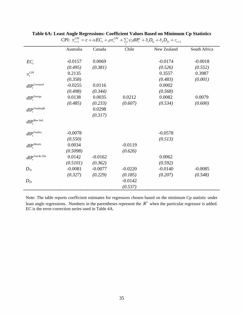
Tables 6A and 6B show the LARS results for CPI- and PPI-inflation. 18 We report

regression specifications chosen by the minimized Cp statistics and the coefficient estimates for the

chosen variables. In addition, the R2’s for the regression after the inclusion of the particular

variable are reported in the parentheses underneath each coefficient estimate. For example, we see

that in the CPI regression for Australia, the first variable selected is the break-date dummy (for

1990Q4), since it has the smallest R2 (0.327) amongst the reported numbers. The next variable

entering is lagged CPI inflation, followed by Energy, the error correction term, Livestock, and 18 We used both the R package lars and Stata to run the LARS regressions reported here.

16

Metals, Fats & Oils, and Textiles, producing a final R2 of 0.55.19 For CPI inflation, the level break

is consistently selected first (with the exception of South Africa), and we note that lagged inflation

is not selected at all for two of the five countries. For PPI inflation, lagged inflation is the first

variable selected for three out of the five countries, but for Australia and Canada, a commodity

price variable is actually the first one selected (the one with the lowest R2). In all cases, at least one,

and up to five, commodity sub-indexes are selected in addition to lagged inflation, the break dates,

or the EC term. The incremental R2 from the sub-indexes are non- negligible either.

Energy remains the most important sub-index in explaining both CPI and PPI inflation,

being significant/selected in all regressions. We note that five of the seven sub-indexes are selected

for the two Australian regressions, as well as for Canadian PPI inflation. In addition, multiple sub-

indexes continue to be important in explaining CPI inflation in Canada, Chile, and New Zealand, as

well as PPI inflation in Chile, New Zealand, and South Africa. Only Energy is selected for

explaining CPI inflation in South Africa, again confirming its overall dominance.

We view these results as additional confirmation that world commodity price sub-indexes

have predictive content for subsequent CPI and PPI inflation a quarter later.20

4. Out-of-Sample Forecasts

This section analyzes the extent to which the commodity indexes can help forecast inflation

rates out-of-sample. We compare the forecast performances of the various commodity price-based

models with two time-series benchmarks: the random walk (RW) and the AR(1) specifications, both

of which are widely adopted in the literature.21 To address the parameter instability issue discussed

19 Regressions that include additional variables that have no reported coefficients deliver larger Cp statistics, and hence are not selected 20 We note that the selected set of variables may not always correspond to the type of products these countries specialize in (Appendix Table 1). For example, while one may expect Chilean CPI inflation to predicted by energy and metal prices, or New Zealand PPI inflation to be linked to the livestock price index, that is not what we find. Our speculation is that since these indexes are all somewhat correlated, the type of multivariate regressions we conduct, given the sample size, may not be powerful enough to select out the precise variables that contain the most relevant information. Since the focus of the paper is not on testing specific structural transmission channels from world commodity prices to inflation, but rather on examining their predictive content for inflation, we do not pursue this issue further. 21 See, for example, Atkeson and Ohanion (2001) and Stock and Watson (2007).

17

in the earlier sections, we first look at forecasts using only the predictors and a rolling window, and

then consider models that explicitly incorporate the estimated break dates identified in Section 2.3,

within a recursive framework.

For each of CPI- and PPI- inflation in the five countries, we consider seven commodity-

index-based models of two general forms. The first type uses matched frequency predictors and is

parallel to the in-sample analyses we have conducted in the earlier sections. These include the

following five out-of-sample specifications (with model names as designated in Table 7):

Sub-Index 1( ) iit t i tE c dlPp y+ = +å (5a)

VECM 1( ) it t t t i t

iE c EC dlPp a rp y+ = + + +å (5b)

FC:AR+7 1

1( ) ( )

8i

t t t i i ti

E c c dlPp rp y+ = + + +å (5c)

Agg Index 1( ) Agg RJt t tE c dlPp y -

+ = + (5d)

AR + Agg Index 1( ) Agg RJt t t tE c dlPp rp y -

+ = + + (5e)

Index i denotes the seven commodity sub-indexes. For the VECM specification above, the error

correction term is re-constructed during each iteration of forecasting, using the cointegration vectors

obtained under dynamic OLS estimation for the particular sub-sample.22 We note that the first two

specifications involve a substantial number of regressors. For the small sample sizes used in the

pseudo out-of-sample exercise, estimation errors are therefore likely to affect forecast accuracy.

We therefore next consider three alternative, more parsimonious specifications. The third equation,

(5c), represents a forecast combination, which is the simple average of the seven univariate

forecasts: 1( )i it t i i tE c dlPp y+ = + using one subindex i at a time in each estimation, together with the

22 Specifically, we regress the log price level, CPI or PPI, on a time trend and the log level of each of the seven commodity price indexes, along with one lead and one lag of their first difference. Due to the small sample sizes and the number of regressors, we do not consider higher orders of leads and lags.

18

AR forecast.23 The last two specifications, (5d) and (5e), use the aggregate commodity price index

instead.

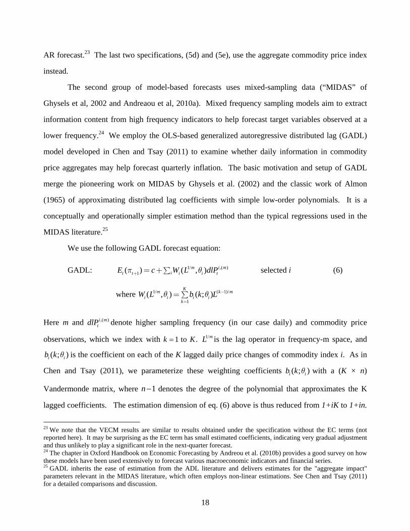
The second group of model-based forecasts uses mixed-sampling data (“MIDAS” of

Ghysels et al, 2002 and Andreaou et al, 2010a). Mixed frequency sampling models aim to extract

information content from high frequency indicators to help forecast target variables observed at a

lower frequency.24 We employ the OLS-based generalized autoregressive distributed lag (GADL)

model developed in Chen and Tsay (2011) to examine whether daily information in commodity

price aggregates may help forecast quarterly inflation. The basic motivation and setup of GADL

merge the pioneering work on MIDAS by Ghysels et al. (2002) and the classic work of Almon

(1965) of approximating distributed lag coefficients with simple low-order polynomials. It is a

conceptually and operationally simpler estimation method than the typical regressions used in the

MIDAS literature.25

We use the following GADL forecast equation:

GADL: 1/ ,( )

1( ) ( , )m i mit t i i tE c W L dlPp q+ = +å selected i (6)

where 1/ ( 1)/

1( , ) ( ; )

Km k m

i i i ik

W L b k Lq q -

== å

Here m and ,( )i mtdlP denote higher sampling frequency (in our case daily) and commodity price

observations, which we index with 1 to .k K 1/mL is the lag operator in frequency-m space, and

( ; )i ib k q is the coefficient on each of the K lagged daily price changes of commodity index i. As in

Chen and Tsay (2011), we parameterize these weighting coefficients ( ; )i ib k q with a (K × n)

Vandermonde matrix, where 1n denotes the degree of the polynomial that approximates the K

lagged coefficients. The estimation dimension of eq. (6) above is thus reduced from 1+iK to 1+in.

23 We note that the VECM results are similar to results obtained under the specification without the EC terms (not reported here). It may be surprising as the EC term has small estimated coefficients, indicating very gradual adjustment and thus unlikely to play a significant role in the next-quarter forecast. 24 The chapter in Oxford Handbook on Economic Forecasting by Andreou et al. (2010b) provides a good survey on how these models have been used extensively to forecast various macroeconomic indicators and financial series. 25 GADL inherits the ease of estimation from the ADL literature and delivers estimates for the "aggregate impact" parameters relevant in the MIDAS literature, which often employs non-linear estimations. See Chen and Tsay (2011) for a detailed comparisons and discussion.

19

We set n = 3 in our forecast analyses below. Given our small sample size in the rolling estimation

procedures (window size = 68), we note that using all seven sub-indexes would stretch the degrees

of freedom. We thus run eq. (6) using only the sub-indexes of Livestock, Energy, Metals, and Fats

& Oils, as these are typically the most statistically significant indexes in the VECM(1) equations for

each country.26 To complement these results, we also employ forecast combination in the mixed-

frequency context in order to use information from all seven sub-indexes. Specifically, we compute

a simple average of the seven univariate GADL forecasts for each i and the AR forecast, as follows:

FC: AR+7 GADL: 1/ ,( )1

1( ) ( ( , ) )

8m i m

t t t i i i ti

E c c W L dlPp rp q+ = + + +å (7)

We conduct GADL forecasts for K = 14, 34, and 54, representing using daily data of roughly three

weeks, a month and a half, and the full quarter respectively. In addition, we also explore adding an

AR term into eq. (7). To conserve space, we report in Table 7 only results for eqs. (6) and (7) using

K = 34. The qualitative conclusions do not differ under the other specifications.27

We compare the forecast errors from the commodity-price-based models against those from

the two following time-series benchmark models, RW and AR(1):

RW 1( )t t tE p p+ = (8a)

AR(1) 1( )t t tE cp rp+ = + (8b)

To address parameter instability, we first adopt the rolling out-of-sample scheme as it is more

robust to the presence of time-varying parameters and requires no explicit assumption as to the

nature of the time variation in the data. We use a rolling window with size equal to 68 quarters to

estimate the model parameters and generate one quarter-ahead forecasts recursively.28 (We note

26 As a robustness check, we also explored GADL forecasts using the top indexes selected by LARS (Table 6). Overall, the forecast performance does not improve upon the results we report. Using all seven indexes in one multi-variate regression, however, does produce larger RMSEs. 27 For example, including an AR term in Eq. (6) significantly improves forecasts for Chile and South African CPI-inflation, but deteriorates the results for the other three countries somewhat. This is likely related to the structural break in the level of inflation discussed earlier. 28 Given that the rolling forecast procedure is quite standard in the literature, we do not describe it here but refer interested readers to Clark and McCracken (2001), Clark and West (2006, 2007) for a theoretical exposition, and Engel,

20

that we also looked at one-year ahead forecasts, but found that the models do not produce better

performance than the one quarter-ahead results we report here.)

Table 7 reports the root mean squared forecast errors (RMSEs) for the two benchmarks and

the RMSE ratios of the seven commodity index based-models relative to the benchmarks. A RMSE

ratio < 1 indicates smaller forecast errors from the particular model. Overall, we see that the

different variations of commodity index-based models, including ones using mixed frequency data,

perform similarly and that based on the RMSE ratio criterion, we don’t observe any one

specification that dominates the others.29 Comparing to the benchmarks, we note that commodity

indexes deliver better forecast performance than the RW forecasts, with the notable exception being

the CPI inflation forecasts for Chile and South Africa. Compared to the AR(1) benchmark, the

models do not generally produce notably smaller RMSEs, a result that is consistent with forecasting

inflation in the US, for example.30 However, we do note that the model produces more than a 15%

improvement in forecasting Australian CPI over AR, and a 5% improvement in a several other

cases.

We next incorporate the break date estimates in Table 2 explicitly into the forecasting

procedure. We consider two specifications, which augment the first two specifications in Table 7

with break dummies:

SubIndex-Rec. 1 1 1 2 2( ) iit t i t t tE c dlP D Dp y d d+ = + + +å (9a)

VECM-Rec. 1 1 1 2 2( ) it t t t i t t t

iE c EC dlP D Dp a rp y d d+ = + + + + +å (9b)

As above, we start the initial estimation using the first 68 observations. Then, instead of

rolling a fixed window of this size, we expand the estimation sample size by one with each

Mark, West (2008), and Chen, Rogoff, and Rossi (2010) for applications. There are no rigorous guidelines for how best to select window size and our choice of 68, while reasonable and generally within the conventional size, given the sample size, is nevertheless arbitrary. We have experimented with different window sizes ranging from 60-82 and the results are not very different. 29 One can conduct formal model comparisons using tests such as the ones discussed in Clark and McCracken (2001). Our goal here is on relative forecast accuracy in pseudo-out-of-sample context. 30 The fact that it is easy to forecast better than RW, but hard to forecast better than AR is not surprising, given that we already observe that the additional predictive power of the sub-indexes in the in-sample regressions are not very large.

21

successive estimation and forecast. The recursive forecasts obtained with explicit break dates are

compared to the RW and AR benchmarks. As is evident from Table 8, the models now produce

much more impressive gains over the benchmarks. For example, commodity-price models now

deliver more than a 25% improvement over the AR(1) forecasts for the Chilean CPI inflation, for

example, and overall, a 10% improvement is a lot more commonplace.

In summary, we see that for both CPI and PPI inflation rates, commodity indexes – whether

the specific selected individual ones or their aggregates – can help provide better forecast for

inflation rates a quarter ahead, though the marginal improvements over an AR specification may not

always be large. Incorporating known structural breaks into the forecast model generally improves

performance. While it is beyond the scope of this paper, we see these results as indicative of the

potential usefulness of combining market-based indicators, such as commodity prices, with

structural variables, such as the output gap or unemployment rates from the Phillips' curve, to

deliver more accurate forecasts.

5. Conclusions

With central banks increasingly basing their monetary policies on some form of Taylor rule

in which the nominal interest rate is adjusted in response to some measure of inflationary pressures,

the question is raised to what degree should the response incorporate changes in asset prices. The

consensus view seems to be that these prices should be taken into account only to the extent that

they reflect underlying inflationary expectations, and therefore may be reasonable predictors of

future inflation. Starting from this viewpoint, this paper has examined the information contained in

sub-indexes of commodity prices, using data for five small commodity-dependent economies. The

motivation for this choice is that commodity prices are asset prices, which such economies can take

as exogenously given, thereby avoiding issues involving simultaneity which would naturally arise in

large economies such as the United States. In addition, by influencing the choice of production

techniques and consumption choices, commodity prices have a direct link to the real economy.31 31 The most widely studied aspect of this element involves the role of oil/energy as an intermediate input, on which an extensive literature exists.

22

The overall message of this paper is the following. Our empirical estimates do suggest that

the information contained in commodity prices can be helpful in predicting both CPI and PPI

inflation. We find this to be encouraging, since the objective of monetary policy is usually directed

toward targeting inflation. Moreover, since different countries are specialized in different

commodity groups, the prices of which although co-moving also follow different dynamic paths,

our findings suggest that disaggregating to sub-indexes is helpful as well.

Having established that the sub-indexes of commodity prices do indeed contain information

that may be useful in predicting inflation and that therefore may form an appropriate component of

monetary policy the natural next step is to add commodity prices to the monetary policy rule itself.

One can then introduce this augmented policy rule into a complete calibrated structural model of a

small open economy and examine the extent to which this additional information does in fact

improve the effectiveness of monetary policy in terms of enhancing macroeconomic performance

and promoting price stability.

Acknowledgements *We would like to thank three anonymous referees for their constructive suggestions on earlier versions and Erica Clower, Han Lian Chang, and Kelvin Wong for excellent research assistance. All remaining errors are our own. Turnovsky’s research was supported in part by the Castor Endowment at the University of Washington.

23

References

Ai, C., A. Chatrath, and F.M. Song, 2006, On the comovement of commodity prices, American

Journal of Agricultural Economics 88, 574-588.

Almon, S., 1965, The distributed lag between capital appropriations and expenditures,

Econometrica 33, 178-196.

Amano, R. and S. van Norden, 1993, A forecasting equation for the Canada-U.S. dollar exchange

rate, The Exchange Rate and the Economy, 201-65, Bank of Canada, Ottawa.

Andreou. E., E. Ghysels, and A. Kourtellos, 2010a, Regression models with mixed sampling

frequencies, Journal of Econometrics 158, 246-261.

Andreou, E., A. Kourtellos and E. Ghysels, 2010b, Forecasting with mixed frequency data in M.P.

Clements and D.F. Hendry (eds.), Oxford Handbook on Economic Forecasting, Oxford

University Press, Oxford UK.

Atkeson, A. and L.E. Ohanian, 2001, Are Phillips curves useful for forecasting inflation? Federal

Reserve Bank of Minneapolis Quarterly Review 25:1, 2-11.

Bai, J., and P. Perron, 1998, Estimating and testing in linear models with multiple structural

changes, Econometrica 66, 47-78.

Bai, J., and P. Perron, 2003, Computation and analysis of multiple structural change models, Journal

of Applied Econometrics 18, 1-22.

Baillie, R.T., 1989, Commodity prices and aggregate inflation: Would a commodity price rule be

worthwhile?, Carnegie-Rochester Conference on Public Policy 31, 185-240.

Bean, C., 2003, Inflation targeting: The UK experience, Bank of England Quarterly Bulletin,

Winter.

Belke, A., I.G. Bordon, and T.W. Hendricks, 2009, Global liquidity and commodity prices: A

cointegrated VAR approach for OECD countries, Ruhr Economic Papers #102.

Bernanke, B. and M. Gertler, 1999, Monetary policy and asset price volatility, Economic Review,

Federal Reserve Bank of Kansas City, issue Q IV, 17-51,

http://www.nber.org/papers/w7559.

24

Bernanke, B. and M. Gertler, 2001, Should central banks respond to movements in asset prices?

American Economic Review, Papers and Proceedings 91, 253-257.

Blomberg, B. and E. Harris, 1995, The commodity-consumer price connection: Fact or fable?

FRBNY Economic Policy Review, October, 21-38.

Cashin, P.A., L. F. Cespedes, and R. Sahay, 2004, Commodity currencies and the real exchange

rate, Journal of Development Economics, 239-268.

Cashin, P. A., J. C. McDermott, and A. M. Scott, 1999, The myth of comoving commodity prices,

IMF Working Paper, G99/8.

Cecchetti, S. G., Genberg, H. and Wadhwani, S., 2002, Asset prices in a flexible inflation targeting

framework, in W.C. Hunter, G.G. Kaufman and M. Pomerleano (eds.) Asset Price Bubbles:

Implications for Monetary, Regulatory, and International Policies, MIT Press, Cambridge,

MA.

Chen, Y-c. and K. S. Rogoff, 2003, Commodity currencies, Journal of International Economics 60,

133-169.

Chen, Y-c, K. S. Rogoff, and B. Rossi, 2010, Can exchange rates forecast commodity prices?

Quarterly Journal of Economics 125, 1145-1194.

Chen, Y-c. and W-J. Tsay, 2011, "Forecasting Commodity Prices with Mixed Frequency Data: An

OLS-Based Generalized ADL Approach" Working paper University of Washington.

Clark, T., and M. McCracken, 2001, Tests of equal forecast accuracy and encompassing for nested

models, Journal of Econometrics 105, 85-110.

Clark, T. and K. D. West, 2006,Using out-of-sample mean squared prediction errors to test the

martingale difference hypothesis, Journal of Econometrics 135, 155-186.

Clark, T. and K.D. West, 2007, Approximately normal tests for equal predictive accuracy in nested

models, Journal of Econometrics 138, 291-311.

Deb, P., P.K. Trivedi, and P. Varangis, 1996, The excess comovement of commodity prices

reconsidered, Journal of Applied Econometrics 11, 275-91.

25

Efron, B., T. Hastie, I. Johnstone, and R. Tibshirani, 2004, Least angle regression, The Annals of

Statistics 32, 407-451.

Elliott, G., T. J. Rothenberg and J. H. Stock, 1996, Efficient tests for an autoregressive unit root,

Econometrica 64, 813-836.

Engel, C., N. Mark, and K.D. West, 2008, Exchange rate models are not as bad as you think, NBER

Macroeconomics Annual 2007, 381-441.

Fuhrer, J, and G. Moore, 1992, Monetary policy rules and the indicator properties of asset prices,

Journal of Monetary Economics 29, 303-336.

Furlong, F. and R. Ingenito, 1996, Commodity prices and inflation, FRBSF Economic Review 2,

27-47.

Ghysels, E., P. Santa-Clara, and R. Valkanov, 2002, The MIDAS touch: Mixed data sampling

regression models, Working paper UNC and UCLA.

Gospodinov, N and S. Ng, 2010, Commodity prices, convenience yields and inflation, Review of

Economics and Statistics (forthcoming).

Hooker, M., 2002, Are oil shocks inflationary? Asymmetric and nonlinear specifications versus

changes in regime, Journal of Money, Credit and Banking 34, 540-561.

Johansen, S., 1991, Estimation and hypothesis testing of cointegration vectors in Gaussian vector

autoregressive models, Econometrica 59, 1551-1580.

Johansen, S. and K. Juselius, 1990, Maximum likelihood estimation and inference on cointegration

– with applications to the demand for money, Oxford Bulletin of Economics and Statistics

52, 169-210.

Johansen, S., R. Mosconi, and B. Nielsen, 2000, Cointegration analysis in the presence of structural

breaks in the deterministic trend, Econometrics Journal 3, 216-249.

Juselius, K., 2006, The Cointegrated VAR Model: Methodology and Applications, Oxford

University Press, Oxford, UK.

Kugler, P., 1991, Common trends, commodity prices and consumer prices, Economics Letters 37,

345-349.

26

Madigan, D. and G. Ridgeway, 2004, Discussion of ‘Least angle regression’ by Efron et al. The

Annals of Statistics 32, 465-469.

Mahdavi, S. and S. Zhou, 1997, Gold and commodity prices as leading indicators of inflation: Tests

of long-run relationship and predictive performance, Journal of Economics and Business 49,

475-489.

Pecchenino, R.A., 1992, Commodity prices and the CPI: Cointegration, information and signal

extraction, International Journal of Forecasting 7, 493-500.

Pindyck, R.S., and J.J. Rotemberg, 1990, The excess co-movement of commodity prices, Economic

Journal 100, 1173-89.

Stock, J. H. and M. W. Watson, 2003, Forecasting output and inflation: The role of asset prices,

Journal of Economic Literature 41, 788-829.

Stock, J.H. and M.W. Watson, 2007, Why has US inflation become harder to forecast? Journal of

Money, Credit, and Banking (Supplement) 39, 3-33.

27

Table 1 A. Summary Statistics for Quarterly Changes in Commodity Sub-Indexes ( i

tdlP )

1983Q1-2010Q3; Annual Rate

Livestock

tdlP EnergytdlP Foodstuff

tdlP .Raw IndtdlP Textiles

tdlP MetaltdlP &Fats Oils

tdlP

Mean 2.43 3.97 2.22 3.30 1.85 5.57 2.81 t-stat 0.76 0.58 0.94 1.23 1.02 1.27 0.68

St. Dev 35.0 73.5 26.3 23.5 19.0 40.3 45.3 1 0.05 -0.06 0.04 0.28 0.05 0.22 0.11

B. Bi-variate Correlations for Quarterly Changes in Commodity Sub-Indexes ( i

tdlP )

i = Livestock

tdlP EnergytdlP Foodstuff

tdlP .Raw IndtdlP Textiles

tdlP MetaltdlP &Fats Oils

tdlPLivestock

tdlP 1.00 (---)

EnergytdlP 0.47 1.00

(0.00) (---) Foodstuffs

tdlP 0.66 0.26 1.00 (0.00) (0.01) (---)

.Raw IndtdlP 0.66 0.46 0.50 1.00

(0.00) (0.00) (0.00) (---) Textiles

tdlP 0.27 0.16 0.21 0.59 1.00 (0.01) (0.09) (0.03) (0.00) (---)

MetalstdlP 0.51 0.42 0.47 0.91 0.34 1.00

(0.00) (0.00) (0.00) (0.00) (0.00) (---) &Fats Oils

tdlP 0.80 0.31 0.79 0.58 0.21 0.48 1.00 (0.00) (0.00) (0.00) (0.00) (0.02) (0.00) (---)

C. Country-Specific Quarterly Inflation Rates

Australia Canada Chile New Zealand S. Africa CPIt

Mean 3.81 2.62 9.74 3.96 8.80 Std. Dev. 3.15 2.37 9.07 4.79 6.30 1 0.52 0.31 0.58 0.62 0.63

PPIt

Mean 3.21 1.88 10.29 3.62 8.65 Std. Dev. 6.30 4.91 14.00 5.60 6.43 1 0.24 0.29 0.43 0.49 0.47

Note: t-stat denotes the HAC t-statistic for testing the hypothesis that the mean is zero. 1 denotes the lag 1 sample autocorrelation. Numbers in the parentheses are the p-values for the null hypothesis that the correlation is zero.

28

Table 2: Country-Specific Break Dates for Inflation Rates 1983Q1-2010Q3; Annual Rate

1 1, 1, 2, , , 1, ,t j t j j ju t T T T j m

Australia Canada Chile New Zealand S. Africa CPIt

No. of Breaks, m 1 1 2 1 1 Date(s) 1990 Q4 1991 Q1 1992 Q1, 1996 Q3 1988 Q1 1993 Q2

1 7.06 4.521 19.3 10.24 12.99

2 2.489 1.809 9.836 2.501 6.26

3 - - 3.567 - -

1 2.684 1.652 8.711 7.253 4.22

2 2.241 2.168 3.883 2.259 3.919

3 - - 3.423 - -

1,1 0.2506 0.056 -0.1529 0.3327 0.2407

1,2 0.238 0.070 0.1404 0.3308 0.4814

1,3 - - 0.3994 - - PPIt

No. of Breaks, m 1 0 2 1 1 Date(s) 1990 Q4 - 1985 Q3, 1991 Q4 1989 Q4 1991 Q1

1 6.371 1.882 29.03 7.045 12.72

2 1.926 - 15.51 2.459 6.932

3 - - 5.799 - -

1 4.397 4.908 15.62 5.62 3.551

2 6.526 - 12.51 5.131 6.607

3 - - 11.22 - -

1,1 -0.2306 0.29 0.2524 0.4852 0.5473

1,2 0.2605 - 0.1379 0.3733 0.3307

1,3 - - 0.245 - -

Note: Number of breaks is determined by minimizing the BIC of the mean shift regression over different values of m. The estimated break dates minimize the sum of squared residuals of the mean shift regression for the given value of m. 1,, and j j j denote the mean, standard deviation and

lag 1 autocorrelation in regime j, respectively.

29

Table 3A: Estimated Cointegrating Vectors Normalized on CPI

0CPI i

it i t tlP c t lP ud b= + + +å where i = 7 sub-indexes

Australia Canada Chile New Zealand South Africa Livestock 0.25221** 0.34088** 14.5639** 0.90933*** 1.18191 [0.12043] [0.13403] [5.76688] [0.27221] [1.24269] Energy -0.16535*** -0.19695*** -9.40018*** -0.51017*** -1.45295*** [0.03260] [0.03704] [1.57441] [0.07199] [0.32482] Foodstuffs 0.89652*** 1.02281*** 44.4937*** 1.51388*** 8.64816*** [0.13544] [0.15081] [6.73260] [0.29628] [1.36710] Raw Ind. -0.19745 -1.37335*** -108.030*** -2.32637** -11.0751*** [0.42520] [0.47786] [21.1002] [0.95626] [4.19963] Textiles 0.17326 0.56083** 52.6546*** 1.11568** 4.08295** [0.20593] [0.23277] [10.5637] [0.46096] [2.04987] Metals 0.17598 0.61959*** 45.2618*** 1.15843*** 4.95458*** [0.17731] [0.19988] [8.80725] [0.39016] [1.77263] Fats & Oils -0.88285*** -0.74473*** -25.8379*** -1.47374*** -5.58774*** [0.08275] [0.09289] [4.50601] [0.19561] [0.88248] Trend 0.00891*** 0.00549*** -0.03104 0.01074*** 0.01722*** [0.00046] [0.00053] [0.03504] [0.00092] [0.00581] LR 14.95

[0.00011] 3.38 [0.06615]

0.05 [0.82306]

8.67 [0.00324]

0.14 [0.70630]

Note: The cointegrating vectors are maximum likelihood estimates normalized on CPI from cointegrated VAR(2) models with one cointegrating vector. LR denotes the likelihood ratio statistic for the presence of a trend in the cointegrating vector. Values in brackets represent standard errors for coefficients and p-values for LR statistics. Asterisks indicate significance at 1% (***), 5% (**), and 10% (*) level. A constant term is included in the estimation (results not reported).

30

Table 3B: Estimated Cointegrating Vectors Normalized on PPI

0PPI i

it i t tlP c t lP ud b= + + +å where i = 7 sub-indexes

Australia Canada Chile New Zealand South Africa Livestock 0.24095** -1.53594 1.13488*** 0.31007* 0.38289 [0.10130] [1.41126] [0.38329] [0.17159] [0.24405] Energy -0.08081*** -1.17431*** -0.60276*** -0.32348*** -0.37823*** [0.02832] [0.38333] [0.10854] [0.04553] [0.06419] Foodstuffs 0.63986*** 11.9125*** 2.06860*** 1.55645*** 1.62214*** [0.12185] [1.63950] [0.42736] [0.20418] [0.27112] Raw Ind. 0.61025* -9.11144* -1.37213 -0.92932 -0.62522 [0.35958] [4.80886] [1.33434] [0.58942] [0.85136] Textiles -0.24083 5.02833** 0.41744 0.31349 0.42811 [0.17520] [2.41721] [0.64584] [0.28484] [0.41830] Metals -0.07586 3.54652* 0.72459 0.52499** 0.34519 [0.14995] [1.98939] [0.55539] [0.24533] [0.35597] Fats & Oils -0.76684 -6.52506*** -1.95686*** -1.15229*** -1.37881*** [0.07107] [1.02967] [0.27456] [0.12599] [0.16770] Trend 0.00606*** 0.01535*** 0.02315*** 0.00878*** 0.02225*** [0.00039] [0.00332] [0.00149] [0.00060] [0.00096] LR 5.48

[0.01921] 0.59 [0.43934]

4.59 [0.03219]

15.14 [0.00000]

4.29 [0.03829]

Note: The cointegrating vectors are maximum likelihood estimates normalized on PPI from cointegrated VAR(2) models with one cointegrating vector. LR denotes the likelihood ratio statistic for the presence of a trend in the cointegrating vector. Values in brackets represent standard errors for coefficients and p-values for LR statistics. Asterisks indicate significance at 1% (***), 5% (**), and 10% (*) level. A constant term is included in the estimation (results not reported).

31

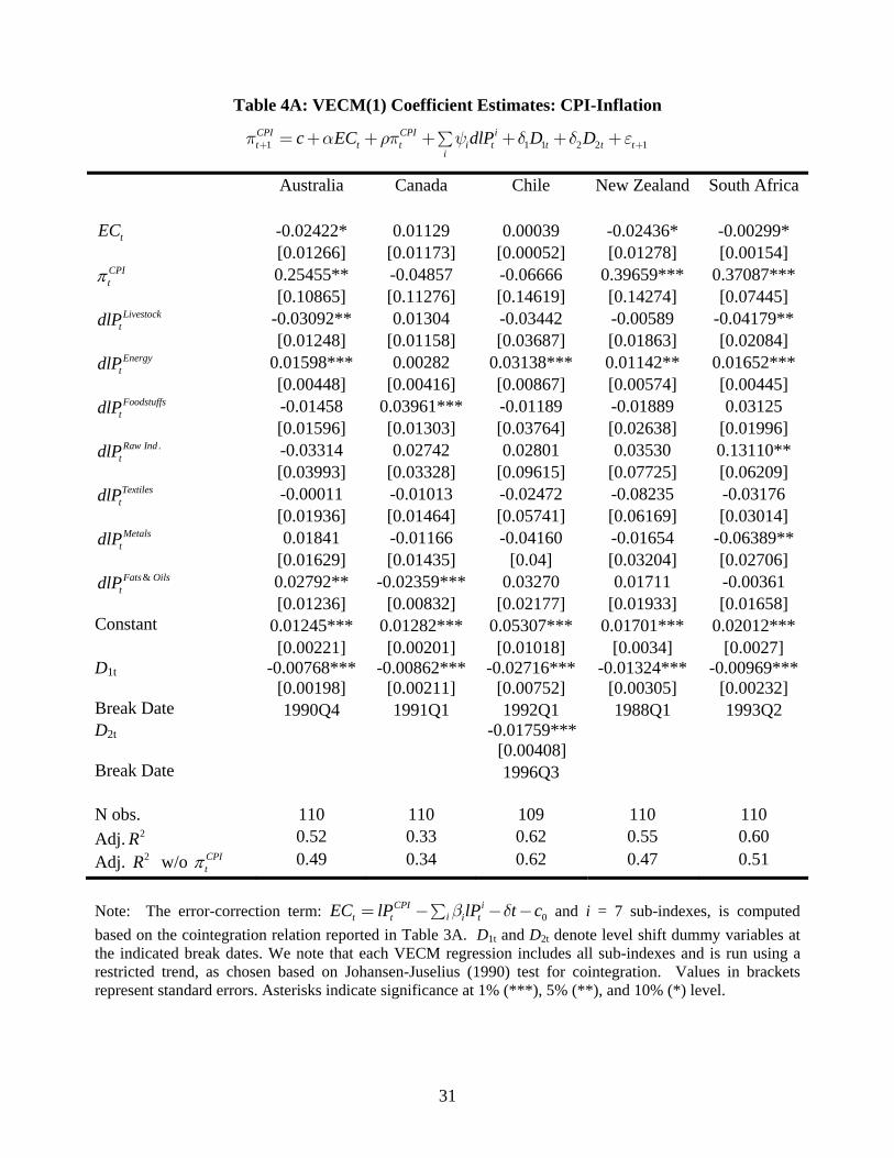
Table 4A: VECM(1) Coefficient Estimates: CPI-Inflation

1 1 1 2 2 1CPI CPI it t t i t t t t

ic EC dlP D Dp a rp y d d e+ += + + + + + +å

Australia Canada Chile New Zealand South Africa

tEC -0.02422* 0.01129 0.00039 -0.02436* -0.00299* [0.01266] [0.01173] [0.00052] [0.01278] [0.00154]

CPIt 0.25455** -0.04857 -0.06666 0.39659*** 0.37087***

[0.10865] [0.11276] [0.14619] [0.14274] [0.07445] Livestock

tdlP -0.03092** 0.01304 -0.03442 -0.00589 -0.04179** [0.01248] [0.01158] [0.03687] [0.01863] [0.02084]

EnergytdlP 0.01598*** 0.00282 0.03138*** 0.01142** 0.01652***

[0.00448] [0.00416] [0.00867] [0.00574] [0.00445] Foodstuffs

tdlP -0.01458 0.03961*** -0.01189 -0.01889 0.03125 [0.01596] [0.01303] [0.03764] [0.02638] [0.01996]

.Raw IndtdlP -0.03314 0.02742 0.02801 0.03530 0.13110**

[0.03993] [0.03328] [0.09615] [0.07725] [0.06209] Textiles

tdlP -0.00011 -0.01013 -0.02472 -0.08235 -0.03176 [0.01936] [0.01464] [0.05741] [0.06169] [0.03014]

MetalstdlP 0.01841 -0.01166 -0.04160 -0.01654 -0.06389**

[0.01629] [0.01435] [0.04] [0.03204] [0.02706] &Fats Oils

tdlP 0.02792** -0.02359*** 0.03270 0.01711 -0.00361 [0.01236] [0.00832] [0.02177] [0.01933] [0.01658]

Constant 0.01245*** 0.01282*** 0.05307*** 0.01701*** 0.02012*** [0.00221] [0.00201] [0.01018] [0.0034] [0.0027]

D1t -0.00768*** -0.00862*** -0.02716*** -0.01324*** -0.00969*** [0.00198] [0.00211] [0.00752] [0.00305] [0.00232]

Break Date 1990Q4 1991Q1 1992Q1 1988Q1 1993Q2 D2t -0.01759***

[0.00408] Break Date 1996Q3 N obs. 110 110 109 110 110

Adj. 2R 0.52 0.33 0.62 0.55 0.60

Adj. 2R w/o CPIt 0.49 0.34 0.62 0.47 0.51

Note: The error-correction term: 0CPI i

it t i tEC lP lP t cb d= - - -å and i = 7 sub-indexes, is computed

based on the cointegration relation reported in Table 3A. D1t and D2t denote level shift dummy variables at the indicated break dates. We note that each VECM regression includes all sub-indexes and is run using a restricted trend, as chosen based on Johansen-Juselius (1990) test for cointegration. Values in brackets represent standard errors. Asterisks indicate significance at 1% (***), 5% (**), and 10% (*) level.

32

Table 4B: VECM(1) Coefficient Estimates: PPI-Inflation

1 1 1 2 2 1PPI PPI it t t i t t t t



tEC -0.04435 0.00155 -0.00004 -0.00277 -0.02693 [0.03644] [0.0021] [0.00596] [0.01542] [0.01981]

PPIt 0.12466 0.20667* 0.25216*** 0.39406*** 0.32985***

[0.1009] [0.12094] [0.08936] [0.10738] [0.10977] Livestock

tdlP -0.00435 -0.05522** 0.11589* 0.01415 -0.01379 [0.0278] [0.02191] [0.06647] [0.02223] [0.03133]

EnergytdlP 0.02541*** 0.01110** 0.04463** 0.02008** 0.01933*

[0.0067] [0.00542] [0.02065] [0.00688] [0.01077] Foodstuffs

tdlP -0.01221 0.09272*** 0.04921 0.04925* 0.04599 [0.04165] [0.02856] [0.07947] [0.02558] [0.03426]

.Raw IndtdlP -0.07546 0.12393 -0.05203 -0.14608* 0.09565

[0.09426] [0.0829] [0.19414] [0.07748] [0.08671] Textiles

tdlP -0.01516 -0.02087 -0.04586 0.02354 -0.04739 [0.03202] [0.03263] [0.09983] [0.03054] [0.03719]

MetalstdlP 0.06088 -0.02616 -0.00546 0.06041* -0.03578

[0.04272] [0.03947] [0.09212] [0.03333] [0.03872] &Fats Oils

tdlP 0.03139 -0.01734 -0.04782 0.00396 -0.00322 [0.0263] [0.01562] [0.05068] [0.01817] [0.02151]

Constant 0.01250*** 0.00323** 0.05755*** 0.01257*** 0.01953*** [0.00266] [0.00113] [0.01681] [0.00283] [0.0041]

D1t -0.00839*** -0.02848* -0.00950*** -0.00754** [0.00305] [0.01565] [0.00302] [0.00349]

Break Date 1990Q4 1985Q3 1989Q4 1991Q1 D2t -0.01922**

[0.00785] Break Date 1991Q4 N obs. 110 110 110 110 110

Adj. 2R 0.29 0.22 0.37 0.40 0.34

Adj. 2R w/o PPIt 0.28 0.20 0.34 0.31 0.26

Note: The error-correction term: 0PPI i

it t i tEC lP lP t cb d= - - -å and i = 7 sub-indexes, is computed

based on the cointegration relation reported in Table 3B. D1t and D2t denote level shift dummy variables at the indicated break dates. We note that each VECM regression includes all sub-indexes and is run using a restricted trend, as chosen based on Johansen-Juselius (1990) test for cointegration. Values in brackets represent standard errors. Asterisks indicate significance at 1% (***), 5% (**), and 10% (*) level.

33

Table 5A: CPI-Inflation Regressions using Aggregate Spot Index

1 1 1 2 2 1CPI CPI Agg Spott t t t t tc dlP D Dp rp y d d e-+ += + + + + +

Australia Canada Chile New Zealand South Africa CPItp 0.17453 0.02253 -0.03368 0.33152* 0.37650***

[0.12168] [0.09839] [0.15375] [0.16954] [0.07962] Agg Spot

tdlP - 0.01614* 0.02392* 0.00119 0.00169 0.01558 [0.00815] [0.01332] [0.03877] [0.01213] [0.01399]

D1t -0.00938*** -0.00685 -0.02427*** -0.01400*** -0.01192*** [0.00204] [0.00106] [0.00631] [0.00381] [0.00198]

Break Date 1990Q4 1991Q1 1992Q1 1988Q1 1993Q2 D2t -0.01584

[0.00362] Break Date 1996Q3 N obs. 110 110 110 110 110

Adj. 2R 0.44 0.31 0.57 0.49 0.56

Adj. 2R w/o CPItp 0.43 0.31 0.57 0.43 0.47

Table 5B: CPI-Inflation Regression using Aggregate Reuters-Jefferies Index

1 1 1 2 2 1CPI CPI Agg RJt t t t t tc dlP D Dp rp y d d e-+ += + + + + +

Australia Canada Chile New Zealand South Africa CPIt 0.16151 0.00404 -0.01989 0.33355** 0.38172***

[0.11964] [0.09283] [0.14314] [0.169363] [0.00291] Agg RJ

tdlP - 0.02026*** 0.02304** 0.01942 0.01372 0.01923 [0.00621] [0.01005] [0.02325] [0.01013] [0.01211]

D1t -0.00953*** -0.00698*** -0.02418 -0.01398 -0.01182 [0.00199] [0.00103] [0.00626] [0.00384] [0.00196]

Break Date 1990Q4 1991Q1 1992Q1 D2t -0.01548

[0.00342] Break Date 1996Q3 N obs. 110 110 110 110 110

Adj. 2R 0.47 0.34 0.57 0.50 0.58

Adj. 2R w/o CPIt 0.46 0.35 0.58 0.43 0.47

Note: D1t and D2t denote level shift dummy variables at the indicated break dates. Model specification is chosen based on Johansen-Juselius (1990) test for cointegration. Values in brackets represent standard errors. Asterisks indicate significance at 1% (***), 5% (**), and 10% (*) level.

34

Table 5C: PPI-Inflation Regressions using Aggregate Spot Index

1 1 1 2 2 1PPI PPI Agg Spott t t t t tc dlP D Dp rp y d d e-+ += + + + + +

Australia Canada Chile New Zealand South Africa PPIt 0.13454 0.19397* 0.28887*** 0.42788*** 0.31903***

[0.09277] [0.10206] [0.09952] [0.10357] [0.11533] Agg Spot

tdlP - 0.10477*** 0.08667*** 0.11614 0.06422** 0.07999** [0.02426] [0.02584] [0.08710] [0.02503] [0.03955]

D1t -0.00967*** -0.02566 -0.00751*** -0.01043 0.002774 [0.01578] [0.00282] [0.00336]

Break Date 1990Q4 1985Q3 1989Q4 1991Q1 D2t -0.01797**

[0.00739] Break Date 1991Q4 N obs. 110 110 110 110 110

Adj. 2R 0.22 0.19 0.32 0.34 0.33

Adj. 2R w/o PPIt 0.21 0.17 0.27 0.18 0.25

Table 5D: PPI-Inflation Regressions using Aggregate Reuters-Jefferies Index

1 1 1 2 2 1PPI PPI Agg RJt t t t t tc dlP D Dp rp y d d e-+ += + + + + +

Australia Canada Chile New Zealand South Africa PPIt 0.08866 0.18627** 0.27518*** 0.39435*** 0.31779***

[0.09291] [0.08598] [0.09413] [0.10140] [0.10404] Agg RJ

tdlP - 0.08689*** 0.07407*** 0.09207 0.05561*** 0.06477** [0.01522] [0.01486] [0.07116] [0.01762] [0.03180]

D1t -0.01021*** -0.02694* -0.00816*** -0.01048*** [0.00276] [0.01525] [0.00282] [0.00316]

Break Date 1990Q4 1985Q3 1991Q1 D2t -0.01791**

0.007435 Break Date 1991Q4 N obs. 110 110 110 110 110

Adj. 2R 0.25 0.24 0.32 0.36 0.34

Adj. 2R w/o PPIt 0.25 0.22 0.28 0.23 0.27

Note: D1t and D2t denote level shift dummy variables at the indicated break dates. Model specification is chosen based on Johansen-Juselius (1990) test for cointegration. Values in brackets represent standard errors. Asterisks indicate significance at 1% (***), 5% (**), and 10% (*) level.

35

Table 6A: Least Angle Regressions: Coefficient Values Based on Minimum Cp Statistics

CPI: 1 1 1 2 2 1CPI CPI it t t i t t t t



tEC -0.0157 0.0069 -0.0174 -0.0018 (0.495) (0.381) (0.526) (0.552)

CPItp 0.2135 0.3557 0.3987

(0.358) (0.483) (0.001) Livestock

tdlP -0.0255 0.0116 0.0002 (0.498) (0.344) (0.568)

EnergytdlP 0.0138 0.0035 0.0212 0.0082 0.0079

(0.485) (0.233) (0.607) (0.534) (0.600) Foodstuffs

tdlP 0.0298 (0.317)

.Raw IndtdlP

Textiles

tdlP -0.0078 -0.0578 (0.550) (0.513)

MetalstdlP 0.0034 -0.0119

(0.5098) (0.626) &Fats Oils

tdlP 0.0142 -0.0162 0.0062 (0.5101) (0.362) (0.592)

D1t -0.0081 -0.0077 -0.0220 -0.0140 -0.0085 (0.327) (0.229) (0.185) (0.207) (0.548) D2t -0.0142 (0.537)

Note: The table reports coefficient estimates for regressors chosen based on the minimum Cp statistic under

least angle regressions. Numbers in the parentheses represent the 2R when the particular regressor is added. EC is the error-correction series used in Table 4A.

36

Table 6B: Least Angle Regressions: Coefficient Values Based on Minimum Cp Statistics

PPI:


tEC -0.0336 0.0006 -0.0214 (0.309) (0.271) (0.393)

PPItp 0.1120 0.2001 0.2382 0.3704 0.3177

(0.248) (0.108) (0.037) (0.153) (0.063) Livestock

tdlP -0.0112 -0.0382 0.0511 -0.0043 (0.254) (0.236) (0.387) (0.257)

EnergytdlP 0.0246 0.0105 0.0365 0.0161 0.0156

(0.038) (0.127) (0.288) (0.222) (0.263) Foodstuffs

tdlP 0.0602 0.0452 0.0383 (0.018) (0.414) (0.236)

.Raw IndtdlP 0.0523 0.0115

(0.077) (0.277) Textiles

tdlP -0.0373 -0.0308 -0.0173 (0.340) (0.405) (0.436)

MetalstdlP 0.0297 -0.0011

(0.082) (0.215) &Fats Oils

tdlP 0.0216 (0.281)

D1t -0.0084 -0.0232 -0.0080 -0.0077 (0.228) (0.189) (0.179) (0.191) D2t -0.0172 (0.036)

Note: The table reports coefficient estimates for regressors chosen based on the minimum Cp statistic under

least angle regressions. Numbers in the parentheses represent the 2R when the particular regressor is added. EC is the error-correction series used in Table 4B.

1 1 1 2 2 1PPI PPI it t t i t t t t


37

Table 7: Out-of-Sample Forecast RMSE Ratios: Models vs. Benchmarks

7A: Australia

CPI PPI I. Benchmark RMSEs

RW 0.0088 0.0225 AR(1) 0.0073 0.0183

II. RMSE Ratios: Matched Frequency Models vs. RW vs. AR vs. RW vs. AR

SubIndex 0.64 0.77 0.71 0.88 VECM 0.73 0.89 0.64 0.78 FC: AR+7 0.69 0.83 0.77 0.94 AR+ Agg Index 0.80 0.97 0.69 0.85 Agg Index 0.66 0.80 0.69 0.85

III. RMSE Ratios: Mixed Frequency GADL Models vs. RW vs. AR vs. RW vs. AR

GADL 0.78 0.94 0.80 0.98 FC: AR+7 GADL 0.71 0.85 0.82 1.01

7B: Canada


RW 0.0094 0.0215 AR(1) 0.0072 0.0174




GADL 0.79 1.04 0.86 1.06 FC: AR+7 GADL 0.74 0.96 0.80 0.99

Note: Window size = 68 (# of forecasts = 40), GADL-MIDAS polynomial n = 3 and Aggregation parameter K =34.

38

7C: Chile

CPI PPI

I. Benchmark RMSEsRW 0.0104 0.0440 AR(1) 0.0113 0.0363




GADL 1.71 1.58 0.84 1.01 FC: AR+7 GADL 1.58 1.46 0.82 0.99

7D: New Zealand


RW 0.0068 0.0195 AR(1) 0.0054 0.0169


SubIndex 0.82 1.03 0.80 0.92 VECM 0.79 0.99 0.76 0.87 FC:AR+7 0.79 0.99 0.85 0.98 AR+ Agg Index 0.77 0.96 0.81 0.93 Agg Index 0.79 0.99 0.81 0.93


GADL 0.83 1.05 0.83 0.96 FC: AR+7 GADL 0.79 0.99 0.87 1.00


39

7E: South Africa


RW 0.0100 0.0251 AR(1) 0.0093 0.0211


SubIndex 1.31 1.41 0.79 0.93 VECM 0.90 0.97 0.78 0.93 FC:AR+7 1.24 1.33 0.83 0.98 AR+ Agg Index 0.94 1.01 0.80 0.95 Agg Index 1.31 1.41 0.81 0.96


GADL 1.27 1.36 0.89 1.06 FC: AR+7 GADL 1.19 1.28 0.86 1.03


40

Table 8: Recursive Out-of-Sample Forecasts with Structural Breaks

CPI PPI A: Australia

AR(1) RMSE- Rec. 0.0074 0.0182

vs. RW vs. AR vs. RW vs. AR SubIndex-Rec. 0.70 0.83 0.73 0.90 VECM-Rec. 0.69 0.82 0.71 0.88

B: Canada

AR(1) RMSE- Rec. 0.0073 0.0173

SubIndex-Rec. 0.72 0.92 0.75 0.93 VECM-Rec. 0.72 0.92 0.75 0.94

C: Chile

AR(1) RMSE- Rec. 0.0135 0.0368


D: New Zealand

AR(1) RMSE- Rec. 0.0060 0.0167


E: South Africa

AR(1) RMSE- Rec. 0.0099 0.0216


Note: Forecasts based on recursive procedure using initial sample size of 68. The forecast models incorportate structural breaks determined in Table 3. See text for detail.

41

Table A.1: Representative Major Commodity Exports by Country

Australia Canada New Zealand Chile South Africa Coking coal Crude Oil Lamb Copper Gold Steaming coal Lumber Wholemeal MP Lumber Platinum Gold Pulp Beef Fruits Coal Iron ore Nat. Gas Aluminum Fish Wheat Beef Cheese Aluminum Newsprint Wool Beef Aluminum Casein Alumina Wheat Fish LNG Nickel Butter Wool Gold Sawn Timber Cotton Zinc Kiwi Copper Copper Skim Milk Product Nickel Coal Logs Sugar Hogs Apples Barley Potash Pulp Zinc Fish Skins Canola Canola Lead Corn Rice Silver

Source: Reserve Bank of Australia, Statistics Canada, Reserve Bank of New Zealand , and authors' calculations

42

Table A.2: Components of the Commodity Price Sub-Indexes

CRB Foodstuffs Hogs, steers, lard, butter, soybean oil, cocoa, corn, Kansas City

wheat, Minneapolis wheat, and sugar

S&P GSCI Energy Crude oil (Brent and WTI), natural gas, heating oil, and gasoline

CBR Raw Industrials Hides, tallow, copper scrap, lead scrap, steel scrap, zinc, tin, burlap, cotton, print cloth, wool tops, rosin, and rubber

CRB Livestock and Products Hides, hogs, lard, steers, and tallow

CRB Metals Copper scrap, lead scrap, steel scrap, tin, and zinc

CRB Textiles and Fibers Burlap, cotton, print cloth, and wool tops

CRB Fats and Oils Butter, cottonseed oil, lard, and tallow

Note: The CRB series combine twenty-two commodities into two major subdivisions (Raw Industrials, and Foodstuffs) and four smaller groups (Metals, Textiles and Fibers, Livestock and Products, and Fats and Oils). The groupings are non-mutually exclusive. Please refer to the Commodity Research Bureau for the relative weights and other details concerning these series. More information about the S&P GSCI Energy series can be found on the Standard and Poor’s website.

43

Figure 1: Log Prices

1982Q4-2010Q3

Sources: The CPI and PPI series are from the International Financial Statistics of the IMF. All of the commodity price indexes are from the Commodity Research Bureau, with the exception of the energy series, which is from the Standard and Poor’s.

1985 1995 2005

2.0

2.5

3.0

3.5

4.0

4.5

5.0

log

pric

e

CPI Series

AustraliaCanadaChileNew ZealandSouth Africa

1985 1995 2005

2.0

3.0

4.0

5.0

log

pric

e

PPI Series

1985 1995 2005

4.0

5.0

6.0

7.0

log

pric

e

Commodity Prices

LIVESTOCKENERGYFOODSTUFFRAWINDUSTTEXTILEMETALFATSANDOIL

44

Figure 2.: CPI and PPI Inflation

1983Q1-2010Q3

Note: Inflation rates are computed as the log-difference of the price level and quoted at an annual rate.

1985 1990 1995 2000 2005 2010

-0.2

0.0

0.2

Index

chan

ge in

log

pric

e

Australia

CPIPPI

1985 1990 1995 2000 2005 2010

-0.1

50.

000.

10

Index

chan

ge in

log

pric

e

Canada

1985 1990 1995 2000 2005 2010

-0.2

0.2

0.6

Index

chan

ge in

log

pric

e

Chile

1985 1990 1995 2000 2005 2010

-0.1

0.1

0.3

Index

chan

ge in

log

pric

e

New Zealand

1985 1990 1995 2000 2005 2010

-0.1

0.1

0.3

Index

chan

ge in

log

pric

e

South Africa

45

Figure 3: Commodity Price Inflation

1983Q1-2010Q3

Note: Inflation rates are computed as the log-difference of the price level and quoted at an annual rate.

-1.5

-0.5

0.5

Liv

est

ock

-3-2

-10

12

3

En

erg

y

-1.0

-0.5

0.0

0.5

Fo

od

stu

ff

1985 1990 1995 2000 2005 2010

-1.0

-0.5

0.0

0.5

Ra

win

du

st

-0.4

0.0

0.4

Te

xtile

-2.0

-1.0

0.0

1.0

Me

tal

1985 1990 1995 2000 2005 2010

-1.5

-0.5

0.5

Fa

tsa

nd

oil

46

Figure 4: Aggregate Commodity Price Series

1983Q1-2010Q3

Note: Agg-Spot is the CRB BLS Spot Index and Agg-RJ is the Reuters/Jefferies CRB Index. Inflation rates are computed as the log-difference of the price level and quoted at an annual rate.

1985 1990 1995 2000 2005 2010

5.4

5.8

6.2

log

pri

ce

Commodity Aggregates Price

Agg-SpotAgg-RJ

1985 1990 1995 2000 2005 2010

-1.5

-0.5

0.5

cha

ng

e in

log

pri

ce

Commodity Aggregates Inflation

47

Figure 5: Structural Change in CPI Inflation

1983Q1-2010Q3

Note: Break dates and mean estimations are obtained using Bai and Perron’s (1998, 2003) multiple-break test methodology, and the number of breaks is chosen based on the BIC statistic. See Section 2.3 for details.

Australia: One breakpoint

Time

log

pric

e ch

ange

1985 1990 1995 2000 2005 2010

0.00

0.10

Canada: One breakpoint

Time

log

pric

e ch

ange

1985 1990 1995 2000 2005 2010

-0.0

50.

05

Chile: Two breakpoints

Time

log

pric

e ch

ange

1985 1990 1995 2000 2005 2010

0.0

0.2

0.4

New Zealand: One breakpoint

Time

log

pric

e ch

ange

1985 1990 1995 2000 2005 2010

0.0

0.1

0.2

0.3

South Africa: One breakpoint

Time

log

pric

e ch

ange

1985 1990 1995 2000 2005 2010

-0.0

50.

050.

15

48

Figure 6: Structural Change in PPI Inflation

1983Q1-2010Q3

Note: Break dates and mean estimations are obtained using Bai and Perron’s (1998, 2003) multiple-break test methodology, and the number of breaks is chosen based on the BIC statistic. See Section 2.3 for details.

Australia: One breakpoint

Time

log

pric

e ch

ange

1985 1990 1995 2000 2005 2010

-0.2

0.0

0.2

Canada: No breakpoint

Time

log

pric

e ch

ange

1985 1990 1995 2000 2005 2010

-0.1

50.

000.

10

Chile: Two breakpoints

Time

log

pric

e ch

ange

1985 1990 1995 2000 2005 2010

-0.2

0.2

0.6

New Zealand: One breakpoint

Time

log

pric

e ch

ange

1985 1990 1995 2000 2005 2010

-0.1

00.

050.

20

South Africa: One breakpoint

Time

log

pric

e ch

ange

1985 1990 1995 2000 2005 2010

-0.1

0.1

0.3

Forecasting Inflation using Commodity Price...

Documents

Transcript of Forecasting Inflation using Commodity Price...