1/21/2010

1

Forecasting Fundamentals

Alessandro Anzalone, Ph.D

Hillsborough Community College, Brandon Campus

Agenda

1. Fundamental Principles of Forecasting2. Major Categories of Forecasts2. Major Categories of Forecasts

1. Qualitative Forecasting2. Quantitative Forecasting — Causal3. Quantitative Forecasting— Time Series

3. Forecast Errors4. Computer Assistance5. References

1/21/2010

2

Fundamental Principles of Forecasting

Forecasting is a technique for using past experiences to project expectations for the future.

Fundamental Principles of Forecasting

http://www.opendemocracy.net/content/articles/260/images/0165_Bendell_cartoon3_240702.gif

1/21/2010

3

Fundamental Principles of Forecasting

Forecasts are almost always wrong. The issue is almost never about whether a forecast is correct or not but never about whether a forecast is correct or not. but instead the focus should be on “how wrong do we expect it to be and on the issue of “how do we plan to accommodate the potential error in the forecast.” Much of the discussion of buffer capacity and/or buffer stock the firm may use is directly related to the size of the y yforecast error.

Fundamental Principles of Forecasting

Forecasts are more accurate for groups or families of items It is usually easier to develop a good forecast for items. It is usually easier to develop a good forecast for a product line than it is for an individual product. as individual product forecasting errors tend to cancel each other out as they are aggregated. It is generally more accurate. for example. to forecast the demand for all family sedans than to forecast the demand for one yparticular model of sedan.

1/21/2010

4

Fundamental Principles of Forecasting

Forecasts are more accurate for shorter time periods. In general there are fewer potential disruptions in the near general. there are fewer potential disruptions in the near future to impact product demand. Demand for extended time periods far into the future are generally less reliable.

Fundamental Principles of Forecasting

Every forecast should include an estimate of error. The first principle indicated the importance to answer the first principle indicated the importance to answer the question. “How wrong is the forecast?” Therefore, an important number that should accompany the forecast is an estimate of the forecast error. To be complete, a good forecast has both the forecast estimate and the estimate of the error.

1/21/2010

5

Fundamental Principles of Forecasting

Forecasts are no substitute for calculated demand. If you have actual demand data for a given time period you have actual demand data for a given time period, you should never make calculations based on the forecast for that same time period. Always use the real data, when available.

Qualitative Forecasting

Qualitative forecasting, as the name implies. are forecasts that are generated from information that does not have a that are generated from information that does not have a well-defined analytic structure. They can he especially useful when no past data is available, such as when a product is new and has no sales history. To he more specific. some of the key characteristics of qualitative forecasting data include:g

1/21/2010

6

Qualitative Forecasting

The forecast is usually based on personal judgment or some external qualitative data.

The forecast tends to be subjective and, since they tend to be The forecast tends to be subjective and, since they tend to be developed from the experience of the people involved, will often be biased based on the potentially optimistic or pessimistic position of those people.

An advantage is that this method often does allow for some fairly rapid results.

In some cases, qualitative forecasts are especially important as they may be the only method available.

These methods are usually used for individual products or product families, seldom for entire markets.

Qualitative Forecasting

1. Market surveys

2. Delphi or panel consensus forecasting2. Delphi or panel consensus forecasting

3. Life cycle analogy forecasting1. What is the time frame? How long will growth and maturity last?2. How rapid will the growth be? How rapid will the decline be?3. How large will the overall demand be, especially during the mature

phase?

4. Informed judgment

1/21/2010

7

Qualitative Forecasting

http://2.bp.blogspot.com/_1V7wnZxPqok/Rybl69viwsI/AAAAAAAAHNI/8DRPTr28Q3o/s400/cartoon+expert.jpg

Qualitative Forecasting

Generic Product Life cycle

http://2.bp.blogspot.com/_0gtnzNvK13Q/R8XNssoA1QI/AAAAAAAAADI/53Z54G2ZLWI/s400/product-life-cycle.png

1/21/2010

8

Quantitative Forecasting — Causal

1. This method is based on the concept of relationship between variables, or the assumption that one measurable variable “causes” the other to change in a predictable fashion.causes the other to change in a predictable fashion.

2. There is an important assumption of causality and that the causal variable can be accurately measured. The measured variable that causes the other to change is frequently called a “leading indicator.” As an example, new housing starts is often used as a leading indicator for developing forecasts for many sectors of the economy.

3. If there are good leading indicators developed, these methods often bring excellent forecasting results.

Quantitative Forecasting — Causal

4. As somewhat of a side benefit, the process of developing the models will often allow the developers of the model to gain additional significant market knowledge. For example, if you are additional significant market knowledge. For example, if you are developing a causal model of vacation travel based on the leading indicator of gasoline prices, there is a good chance you will gain knowledge about both the mechanisms that control gasoline prices as well as the patterns of typical vacation travel.

5. These methods are seldom used for product, but more commonly used for entire markets or industries,

6. The methods are often time-consuming and very expensive to develop, primarily because of developing the relationships and obtaining the causal data.

1/21/2010

9

Quantitative Forecasting — Causal

Some of the more common methods of causal forecasting are given as:

Input—output models. These can be very large and complex models, as they examine the flow of goods and services throughout the entire economy. As such, they require a substantial quantity of data, making them expensive and time-consuming to develop. They are generally used to project needs for entire markets or segments of the economy, and not for specific products.

Econometric models. These models involve a statistical analysis of various sectors of the economy. Their use is similar to the input—output models.

Quantitative Forecasting — Causal

Simulation models. Simulating sectors of the economy on computers are growing in popularity and use with the development of ever more powerful and less expensive computers and computer more powerful and less expensive computers and computer simulation models. They can be used for individual products, but once again gathering the data tends to be expensive and time-consuming. The real value of these models is that they are fast and economical to use once the data has “populated” the model.

1/21/2010

10

Quantitative Forecasting — Causal

Regression. A statistical method to develop a defined analytic relationship between two or more variables. The assumption, as with other causal models, is that one variable “causes” the other with other causal models, is that one variable causes the other to move. Often the independent, or causal, variable is called a leading indicator. A common example is when the news reports on housing starts, since that is often a leading indicator of the amount of economic activity in several related markets. Since they are based on external data, causal forecasting methods are sometimes called extrinsic forecasts.

Quantitative Forecasting— Time Series

Time-series forecasts are among the most commonly used for forecasting packages linked to product demand forecasts. They all essentially have one common assumption. That assumption is all essentially have one common assumption. That assumption is that past demand follows some pattern, and that if that pattern can be analyzed it can be used to develop projections for future demand, assuming the pattern continues in roughly the same manner. Ultimately that implies the assumption that the only real independent variable in the time series forecast is time. Since they are based on internal data (sales), they are sometimes called intrinsic forecasts.

1/21/2010

11

Quantitative Forecasting— Time Series

Most time series forecasting models attempt to mathematically capture the underlying patterns of past demand.

1. Random pattern2. Trend pattern3. Seasonal Pattern

Quantitative Forecasting— Time Series

1/21/2010

12

Quantitative Forecasting— Time Series

Quantitative Forecasting— Time Series

1/21/2010

13

Quantitative Forecasting— Time Series

Quantitative Forecasting— Time Series

Simple moving averages are as the name implies. nothing more than the mathematical average of the last several periods of actual demand. They take the form:actual demand. They take the form:

Where:F is the forecastt is the current time period meaning Fi is the forecast for the current

time periodAi is the actual demand in period t, andn is the number of periods being used.

1/21/2010

14

Quantitative Forecasting— Time Series

Quantitative Forecasting— Time Series

1/21/2010

15

Quantitative Forecasting— Time Series

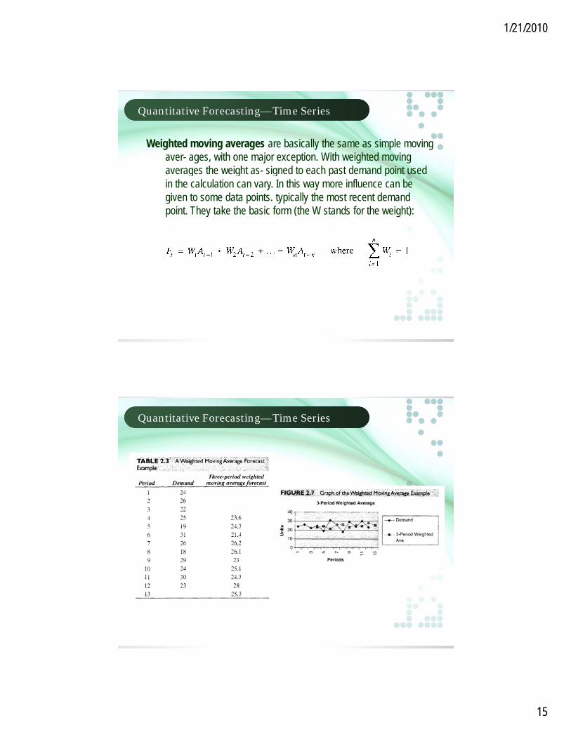
Weighted moving averages are basically the same as simple moving aver- ages, with one major exception. With weighted moving averages the weight as- signed to each past demand point used averages the weight as signed to each past demand point used in the calculation can vary. In this way more influence can be given to some data points. typically the most recent demand point. They take the basic form (the W stands for the weight):

Quantitative Forecasting— Time Series

1/21/2010

16

Quantitative Forecasting— Time Series

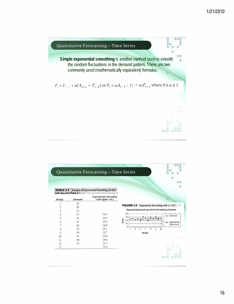
Simple exponential smoothing is another method used to smooth the random fluctuations in the demand pattern. There are two commonly used (mathematically equivalent) formulas:commonly used (mathematically equivalent) formulas:

Quantitative Forecasting— Time Series

1/21/2010

17

Quantitative Forecasting— Time Series

Quantitative Forecasting— Time Series

1/21/2010

18

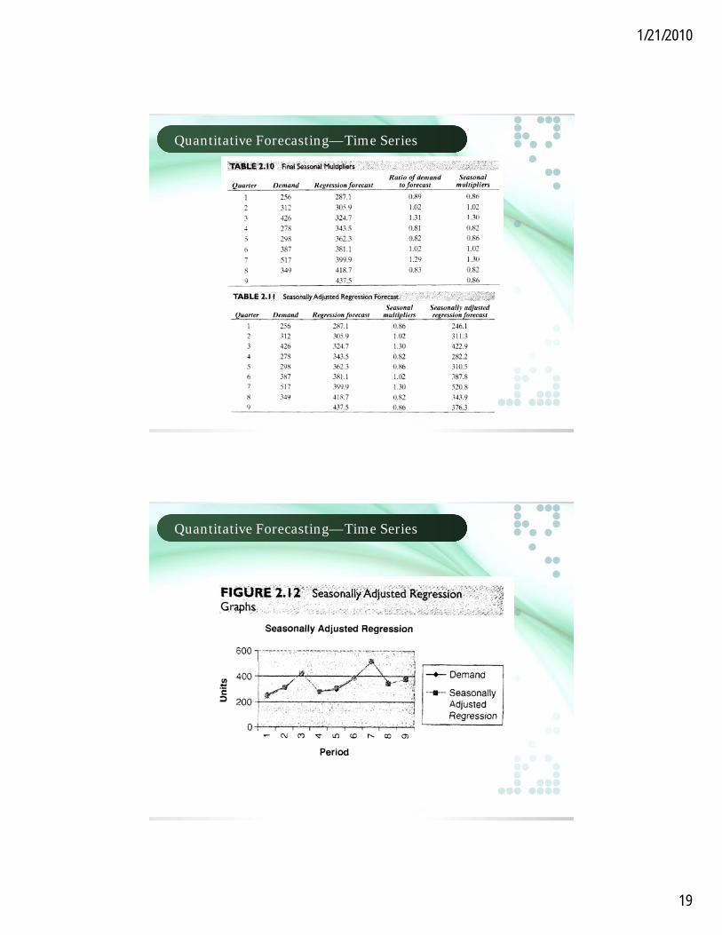
Quantitative Forecasting— Time Series

Regression has sometimes been called the “line of best fit.” It is a statistical technique to try to fit a line from a set of points by using the smallest total squared error between the actual points and the the smallest total squared error between the actual points and the points on the line. A particular value for regression is to determine trend line equations.

Quantitative Forecasting— Time Series

1/21/2010

19

Quantitative Forecasting— Time Series

Quantitative Forecasting— Time Series

1/21/2010

20

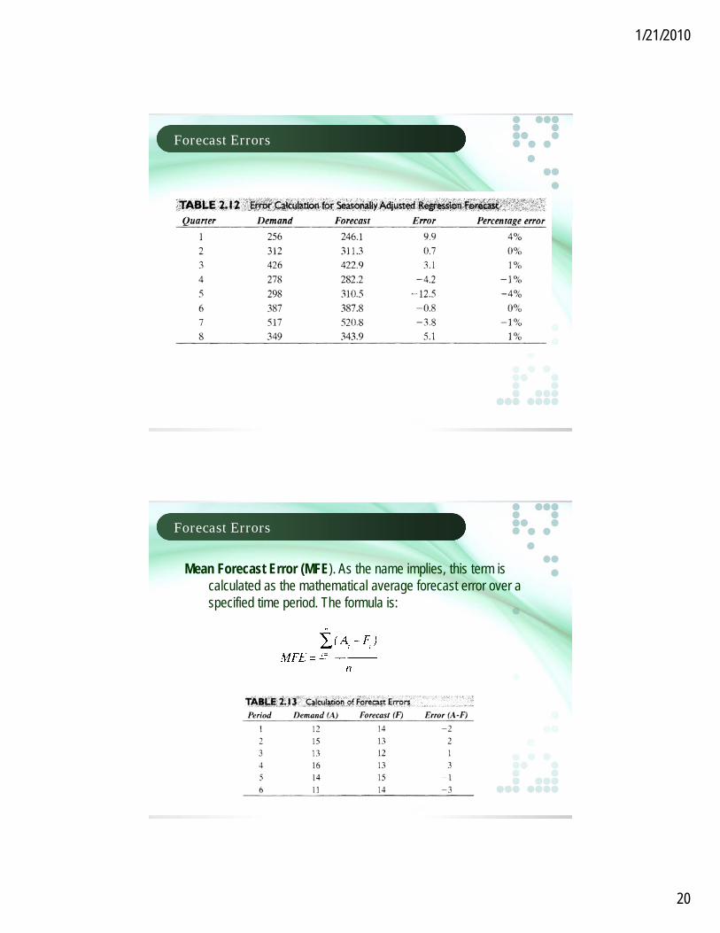
Forecast Errors

Forecast Errors

Mean Forecast Error (MFE). As the name implies, this term is calculated as the mathematical average forecast error over a specified time period. The formula is:specified time period. The formula is:

1/21/2010

21

Forecast Errors

Mean Absolute Deviation (MAD). The formula is again given as the name of the term. It literally means the average of the mathematical absolute deviations of the forecast errors mathematical absolute deviations of the forecast errors (deviations). The formula is, therefore:

Forecast Errors

Tracking Signal. Similar to the concept of control limits for statistical process control charts, the tracking signal provides a somewhat subjective limit for the forecasting method to go “off track” before subjective limit for the forecasting method to go off track before some action is taken. It is calculated from the MFE and the MAD:

1/21/2010

22

Computer Assistance

A demand pattern for 10 periods for a certain product was given as 127. 113. 121, 123. 117. 109. 131. 115. 127. and 118. Forecast the demand for period 11 using each of the following methods: a the demand for period 11 using each of the following methods: a 3-month moving average: a 3-month weighted moving average using weights of 0.2, 0.3, and 0.5; exponential smoothing with a smoothing constant of 0.3; and linear regression. Compute the MAD for each method to determine which method would be preferable under the circumstances. Also calculate the bias in the data, if any, for all four methods, and explain the meaning.

Computer Assistance

1/21/2010

23

References

1. Stephen N. Chapman, The Fundamentals of Production Planning and Control, Prentice Hall, 2006, ISBN-13: 978-0130176158.

2 http://www statpac com/research-papers/forecasting htm2. http://www.statpac.com/research papers/forecasting.htm3. http://www.demandmgmt.com/?q=home/white-papers/5-ways-improve-your-

forecast-accuracy4. http://home.ubalt.edu/ntsbarsh/business-stat/otherapplets/MeasurAccur.htm5. http://www.salesvantage.com/article/628/The-Key-to-Accurate-Sales-

Forecasting