LEARNING OBJECTIVES

After completing this chapter, students will be able to:

1. Understand and know wnen to use various families of forecasting models.

2. Compare moving averages, exponential smoothing, and other time-series models.

3. Seasonally adjust data.

5.1 Introduction

5.2 Types of Forecasting Models

5.3 Components of a Time Series

5.4 Measures of Forecast Accuracy

5.5 Forecasting Models-Random Variations Only

Forecasting

4. Understand Delphi and other qualitative decision­making approaches.

5. Compute a variety ot..error measures.

5.6 Forecasting Models-Trend and Random Variations

5.7 Adjusting for Seasonal Variations

5.8 Forecasting Models-Trend, Seasonal, and Random Variations

5.9 Monitoring and Controlling Forecasts

Summary • Glossary ~ Key Fquations • Solved Problems • Self-Test • Discussion Questions and Problems • Internet Homework Problems • Case Study: Forecasting Attendance at SWU Football Games • Case Study: Forecasting Montllly Sales • Internet Case Study • Bibliography

149

150 CHAPTER 5 • FORECASTING

5.1 Introduction

Every day, managers make decisions without knowing what will happen in the future. Inventory is ordered though no one knows what sales will be, new equipment is purchased though no one knows the demand for products, and investments are made though no one knows what profits will be. Managers are always trying to reduce this uncertainty and to make better estimates of what will happen in the future. Accomplishing this is the main purpose of forecasting.

There are many ways to forecast the future. In numerous firms (especially smaller ones), the entire process is subjective, involving seat-of-the-pants methods, intuition, and years of experience.

There are also more formal forecasting techniques, both quantitative and qualitative in nature. The primary focus of this chapter will be understanding time-series models and deter­mining which model works best with a particular set of data.

5.2 Types of Forecasting Models

FIGURE 5.1 Forecasting Models

Figure 5.1 lists some of the more common forecasting models, and these are categorized by the type of model. The first category involves qualitative models, while the others are quantitative in nature and use mathematical models to develop better forecasts.

Qualitative Models Qualitative models are forecasting techniques based on judgmental or subjective factors. When a totally new product such as the iPad is introduced, forecasting demand is very difficult due to the lack of any historical sales data on that particular product or on similar products. The company must rely on expert opinion, individual experiences and judgment, and other subjective factors.

Here is a brief overview of four different qualitative forecasting techniques:

1. Delphi method. This iterative group process allows experts, who may be located in differ­ent places, to make forecasts. There are three different types of participants in the Delphi process: decision makers, staff personnel, and respon~nts. The decision-making group usually consists of 5 to 10 experts who will be making the actual forecast. The staff person­nel assist the decision makers by preparing, distributing, collecting, and summarizing a series of questionnaires and survey results. The respondents are a group of people whose judgments are valued ~d are being sought. This group provides inputs to the decision makers before the forecast is made.

Qualitative Models

Delphi Method

Jury of Executive Opinion

Sales Force Composite

Consumer Market Survey

Forecasting Techniques

Time-Series Methods

Moving Averages

Exponential Smoothing

Trend Projections

Decomposition

Causal Methods

Regression Analysis

Multiple Regression

Overview of four qualitative or judgmental approaches: Delphi, jury of executive opinion, sales force composite, and consumer market survey.

5.3 COMPONENTS OF A TIME-SERIES 151

In the Delphi method, when the results of the first questionnaire are obtained, the results are summarized and the questionnaire is modified. Both the summary of the re­sults and the new questionnaire are then sent to the same respondents for a new round of responses. The respondents, upon seeing the results from the fust questionnaire, may view things differently and may modify their original responses. This process is repeated with the hope that a consensus is reached.

2. Jury of executive opinion. This method takes the opinions of a small group of high-level managers, often in combination with statistical models, and results in a group estimate of demand.

3. Sales force composite. In this approach, each salesperson estimates what sales will be in his or her region; these forecasts are reviewed to ensure that they are realistic and are then combined at the district and national levels to reach an overall forecast.

4. Consumer market survey. This method solicits input from customers or potential customers regarding their future purchasing plans. It can help not only in preparing a forecast but also in improving product design and planning for new products.

Causal Models A variety of quantitative forecasting models are available when past numerical. data are available. Forecasting models are identified as causal models if the variable to be forecast is influenced by or correlated with other variables included in the model. For example, daily sales of bottled water might depend on the average temperature, the average humidity, and so on. A causal model would include factors such as these in the mathematical model. Regression models (see Chapter 4) and other more complex models would be classified as causal models.

Time-Series Models Time series are also quantitative models, and many time-series methods are available. A time~ series model is a forecasting technique that attempts to predict the future values of a variable by using only historical data on that one variable. These models are extrapolations of past values of that series. While other factors may have influenced these past values, the impact of those other factors is captured in the previous values of the variabl~eing predicted. Thus, if we are fore­casting weekly sales for lawn mowers, we use the past weekly sales for lawn mowers in making the forecast for future sales, ignoring other factors such as the economy, competition, and even the selling price of the lawn mowers.

~· ...t

5.3 Components of a Time-Series .,.

A time series is sequence of values recorded at successive intervals of time. The intervals can be days, weeks, months, years, or other time unit. Examples include weekly sales of HP personal computers, quarterly earnings reports of Microsoft Corporation, daily shipments of Eveready batteries, and annual U.S. consumer price indices. A time series may consist of four possible components-trend, seasonal, cyclical, and random.

The trend (T) component is the general upward or downward movement of the data over a relatively long period of time. For example, total sales for a company may be increasing con­sistently over time. The consumer price index, one measure of inflation, is increasing over time. While consistent upward (or downward) movements are indicative of a trend, there may be a positive (or negative) trend present in a time series and yet the values do not increase (or de­crease) in every time period. There may be an occasional movement that seems inconsistent with the trend due to random or other fluctuations.

Figure 5.2 shows scatter diagrams for several time series. The data for all the series are quar­terly, and there are four years of data. Series 3 has both trend and random components present.

The seasonal (S) component is a pattern of fluctuations above or below an average value that repeats at regular intervals. For example, with monthly sales data on snow blowers, sales tend to be high in December and January and lower in summer months and this pattern is ex­pected to repeat every year. Quarterly sales for a consumer electronics store may be higher in the fourth quarter of every year and lower in other quarters. Daily sales in a retail store may be higher on Saturdays than on other days of the week. Hourly sales in a fast-food restaurant are usually expected to be higher around the lunch hour and the dinner hour, while other times are not as busy. Series 2 in Figure 5.2 illustrates seasonal variations for quarterly data.

152 CHAPTER 5 • FORECASTING

FIGURE 5.2 Scatter Diagram for Four Time Series of Quarterly Data

FIGURE 5.3 Scatter Diagram of a Times Series with Cyclical and Random Components

rJ) Q) (ij en

Series 4: Trend, Seasonal and Random Variations 0

0 0 ••••••••• -··

----~ ------·· t>·--0 0 ·-··

0 0

0 o-------- cr ···· _ ......... ...... -·--o­... -....

0 ........ --0 0 Series 3: Trend and Random Variations

________ 9.-··o ~--·0' 0 ... .o-··"::1····

o.-··er···o Q, 9--··Cf'·--... -o··-- ---o··-·;

Series 2: Seasonal Variations Only

0 0 0 0 0 o···-o······················-o···tr·················-o·············o ..... 0 0 0 0 0

Series 1: Random Variations Only

2 3 4 5 6 7 8 9 10 11 12 13 14 15 16

. Time Period (Quarters)

If a seasonal component is present in a set of data, the number of seasons depends on the type of data. With quarterly data, there are four seasons because there are four quarters in a year. With monthly data, there would be 12 seasons because thert'are 12 months in a year. With daily sale& data for a retail store that is open seven days a week, there would be seven seasons. With hourly data, there could be 24 seasons if the business is open 24 hours a day.

A cyclical (C) compo"'pt of a time series is a pattern in annual data that tends to repeat every several years. The cyc1i&,u component of a time series is only used when making very long-range forecasts, and it is usually associated with the business cycle. Sales or economic ac­tivity might reach a peak and then begin to recede and contract, reaching a bottom or trough. At some point after the trough is reached, activity would pick up as recovery and expansion takes place. A new peak would be reached and the cycle would begin again. Figure 5.3 shows 16 years of annual data for a time series that has a cyclical as well as a random component.

While a time series with cyclical variations and a time series with seasonal variations may look similar on a graph, cyclical variations tend to be irregular in length (from a few years to

rJ) Q)

~

0 2

•

4 6

•

8 10 12 14 16 18 Time Period (Years)

5.4 MEASURES OF FORECAST ACCURACY 153

10 or more y,ears) and magnitude, and they are very difficult to predict. Seasonal variations are very consistent in length and magnitude, are much shorter as the seasons repeat in a year or less, and are much easier to predict. The forecasting models presented in this chapter will be for short­range or medium-range forecasts and the cyclical component will not be included in these models.

The random (R) component consists of irregular, unpredictable variations in a time series. Any variation in a times series that cannot be attributed to trend, seasonal, or cyclical variations would fall into this category. If data for a time series tends to be level with no discernible trend or seasonal pattern, random variations would be the cause for any changes from one time period to the next. Series 1 in Figure 5.2 is an example of a time series with only a random component.

There are two general forms of time-series models in statistics. The first is a multiplicative model, which assumes that demand is the product of the four components. It is stated as follows:

Demand = T X S X C X R

An additive model adds the components together to provide an estimate. Multiple regres­sion is often used to develop additive models. This additive relationship is stated as follows:

Demand = T + S + C + R

There are other models that may be a combination of these. For example, one of the com­ponents (such as trend) might be additive while another (such as seasonality) could be multi­plicative. Understanding the components of a time series will help in selecting an appropriate forecasting technique to use. The methods presented in this chapter will be grouped according to the components considered when the forecast is developed.

5.4 Measures of Forecast Accuracy

TABLE 5.1 Computing the Mean Absolute Deviation (MAD)

We discuss several different forecasting models in this chapter. To see how well one model works, or to compare that model with other !D-odels, the forecast values are compared with the actual or observed values. The forecast error (or deviation) is defined as follows:

Forecast error = Actual value - Forecast value

One measure of accuracy is the mean absolute deviation f.MAD). This is computed by tak­ing the. sum of the absolute values of the individual forecast errors and dividing by the numbers of errors (n):

2

3

4

5

6

7

8

9

10

11

): ~D = ~ I forecast error I n

110

100 110

120 100

140 120

170 140

150 170

160 150

190 160

200 190

190 200

190

(5-1)

IIOO- 110 1 = 10

1120- 100 1 = 20

1140 - 120 ~ = 20

1170- 140 1 = 30

It 5o - t7o I = 20

l t6o - t5o 1 = 10

1190 - 160 1 = 3o

1200- 190 1 = 10

1190- 200 1 = 10

Sum of I errors I = 160

MAD=-= 160/ 9 = 17.8

154 CHAPTER 5 • FORECASTING

To illustrate how to compute the measures of accuracy, the na'ive model will be used to fore­cast one period into the future. The naive model does not attempt to address any of the com­ponents of a time series, but it is very quick and easy to use. A naive forecast for the next time period is the actual value that was observed in the current time period. For example, suppose someone asked you to forecast the high temperature in your city for tomorrow. If you forecast the temperature to be whatever the high temperature is today, your forecast would be a na1ve forecast. This technique is often used if a forecast is needed quickly and accuracy is not a major concern.

Consider the Walker Distributors sales of wireless speakers shown in Table 5 .1. Suppose that in the past, Walker had forecast sales for each month to be the sales that were actually achieved in

Hurricane Landfall Location Forecasts and the Mean Absolute Deviation

S cientists at the National Hurricane Center (NHC) of the Na­tional Weather Service have the very difficult job of predicting where the eye of a hurricane will hit land. Accurate forecasts are extremely important to coastal businesses and residents who need to prepare for a storm or perhaps even evacuate. They are also important to local government officials, law enforcement agencies, and other emergency responders who will provide help once a storm has passed. Over the years, the NHC has tremen­dously improved the forecast accuracy (measured by the mean absolute deviation [MAD]) in predicting the actual landfall loca­tion for hurricanes that originate in the Atlantic Ocean.

are recorded when a hurricane is 72 hours, 48. hours, 36 hours, 24 hours, and 12 hours away from actually reaching land. Once the hurricane has come ashore, these forecasts are compared to the actual landfall location, and the error (in miles) is recorded. At the end of the hurricane season, the errors for all the hurricanes in that year are used to calculate the MAD for each type of fore­cast (12 hours away, 24 hours away, etc.). The graph below shows how the landfall location forecast has improved since 1989. Dur­ing the early 1990s, the landfall forecast when the hurricane was 48 hours away had an MAD close to 200 miles; in 2009, this number was down to about 75 miles. Clearly, there has been vast improvement in forecast accuracy, and this trend is continuing.

The NHC provides forecasts and periodic updates of where the hurricane eye will hit land. Such landfall location predictions Source: Based on National Hufncane Center, http://www.nhc.noaa.gov.

MAD (in Miles) of Hurrican.e Landfall Location ...

Forecasf1989-2009

450

400

350 J

......... I \ 300 I

~ j Ill 250 \ ---12 hours out ~ \ .....__ 24 hours out :E 200 ••

--36 hours out 150 --48 hours out

100 --- 72 hours out

50

0

1989 1994 1999 2004 2009

Year

Defining the Problem

j Developing

a Model

j Acquiring Input Data

j Developing a Solution

l Testing the

Solution

! Analyzing

the Results

! Implementing the Results

The nai've forecast for the next period is the actual value observed in the current period.

5.4 MEASURES OF FORECAST ACCURACY 155

Defining the Problem

Forecasting at Tupperware International

To drive production at each of Tupperware's 15 plants in the United States, Latin America, Africa, Europe, and Asia, the firm needs accurate forecasts of demand for its products.

Developing a Model A variety of statistical models are used, including moving averages, exponential smoothing, and regression analysis. Qualitative analysis is also employed in the process.

Acquiring Input Data At world headquarters in Orlando, Florida, huge databases are maintained that map the sales of each product, the test market results of each new product (since 20% of the firm's sales come from products less than 2 years old), and where each product falls in its own life cycle.

Developing a Solution Each of Tupperware's 50 profit centers worldwide develops computerized monthly, quarterly, and 12-month sales projections. These are aggregated by region and then globally.

Testing the Solution Reviews of these forecasts take place in sales, mijrketing, finance, and production departments.

Analyzing the Results Participating managers analyze forecasts with Tupperware's version of a "jury of executive opinion."

Implementing the Results. • .._ Forecasts are used to schedule ma(eri ls, equipment, and personnel at each plant.

Source: Interviews by the authors with Tupperware executives.

the previous month. Table 5.1 gives these forecasts as well as the absolute value of the errors. In forecasting for the next time period (month 11), the forecast would be 190. Notice that there is no error computed for month 1 since there was no forecast for this month, and there is ·DO error for month 11 since the actual value of this is not yet known. Thus, the number of errors (n) is 9.

From this, we see the following:

~ I forecast error I 160 MAD= =- = 17.8

n 9

This means that on the average, each forecast missed the actual value by 17.8 units. Other measures of the accuracy of historical errors ·in forecasting are sometimes used be­

sides the MAD. One of the most common is the mean squared error (MSE), which is the aver­age of the squared errors:*

~( error)2

MSE=--­n

(5-2)

'In regression analysis, the MSE formula is usually adjusted to provide an unbiased estimator of the error variance. Throughout this chapter, we will use the formula provided here.

1'56 CHAPTER 5 • FORECASTING

Three common measures of error are MAD, MSE, and MAPE. Bias gives the average error and may be positive or negative.

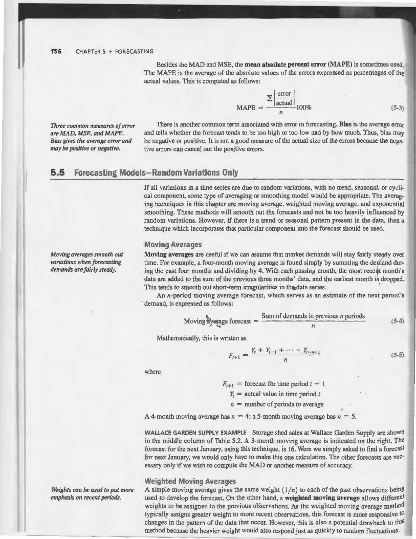
Besides the MAD and MSE, the mean absolute percent error (MAPE) is sometimes used. The MAPE is the average of the absolute values of the errors expressed as percentages of the actual values. This is computed as follows:

~I error I MAPE = actual 100%

n (5·3)

There is another common term associated with error in forecasting. Bias is the average error and tells whether the forecast tends to be too high or too low and by how much. Thus, bias may be negative or positive. It is not a good measure of the actual size of the errors because the nega­tive errors can cancel out the positive errors.

5.5 Forecasting Models-Random Variations Only

Moving averages smooth out variations when forecasting demands are fairly steady.

Weights can be used to put more emplulsis on recent periods.

If all variations in a time series are due to random variations, with no tren~. seasonal, or cycli­cal component, some type of averaging or smoothing model would be appropriate. The averag­ing techniques in this chapter are moving average, weighted moving average, and exponential smoothing. These methods will smooth out the forecasts and not be too heavily influenced by random variations. However, if there is a trend or seasonal pattern present in the data, then a technique which incorporates that particular component into the forecast should be used.

Moving Averages Moving averages are useful if we can assume that market demands will stay fairly s~e y over time. For example, a four-month moving average is found simply by summing the de and dur­ing the past four months and dividing by 4. With each passing month, the most rece t month's data are added to the sum of the previous three months' data, and the earliest month i dropped. This tends to smooth out short-term irregularities in thq.data series.

An n-period moving average forecast, which serves as an estimate of the next period's · demand, is expressed as follows:

' Sum of demands in previous n periods Movin-uf!Varage forecast = (5-4)

"' .. ..._ n

Mathematically, this is written as

where

fr + fr- 1 + .. · + fr-n+1 Fr+l = ~--~~------~~

n

Ft+ 1 = forecast for time period t + 1

Yr = actual value in time period t

n = number of periods to average

A 4-month moving average has n = 4; a 5-month moving average has n = 5.

(5-5)

WALLACE GARDEN SUPPLY EXAMPLE Storage shed sales at Wallace Garden Supply are shown in the middle column of Table 5.2. A 3-month moving average is indicated on the right. The forecast for the next January, using this technique, is 16. Were we simply asked to find a forecast for next January, we would only have to make this one calculation. The other forecasts are nec­essary only if we wish to compute the MAD or another measure of accuracy.

Weighted Moving Averages A simple moving average gives the same weight (1/n) to each of the past observations being used to develop the forecast. On the other hand, a weighted moving average allows different weights to be assigned to the previous ob'servations. As the weighted moving average method typically assigns greater weight to more recent observations, this forecast is more responsive to changes in the pattern of the data that occur. However, this is also a potential drawback to thiS method because the heavier weight would also respond just as quickly to random fluctuations.

fABLE 5.2 ...

Wallace Garden Supply shed Sales

5.5 FORECASTING MODELS-RANDOM VARIATIONS ONLY 157

January

February 12 i 1 March 13 + April 16 ) + 12 + 3)/ 3 = 11.67

May 19 (12 + 13 + 16) / 3 = 13.67

June 23 (13 + ,. + ,.)rt·.oo July 26 (16 + 19 + 23) 3 = 19.33

August 30 (19 + 23 + 26) 3 = 22.67

September 28 (23 + 26 + 30) / 3 = 26.33

October 18 (26 + 30 + 28) / 3 = 28.00

November 16 (30 + 28 + 18) / 3 = 25.33

December 14 (28 + 18 + 16) / 3 = 20.67

January (18 + 16 + 14) / 3 = 16.00

A weighted moving average may be expressed as

L (Weight in period i) (Actual value in period i) ~+I = --~~----~--~~--------~----~

L(Weights) (5-6)

Mathematically, this is

(5-7)

where

wi = weight for ith observation

Wallace Garden Suppl~ ;\)cides to use a 3-month weighted moving average forecast with weights of 3 for the most recent ~servation, 2 for the next observation, and 1 for the most dis­tant observation. This would be implemented as follows:

Last month

· / 2 2 months ago

/ 1 ~ 3 months ago

Q) X Sales last month +CD X Sales 2 months ago +CD X Sales 3 months ago

®--___. Sum of the weights

The results of the Wallace Garden Supply weighted average forecast are shown in Table 5.3. In this particular forecasting situation, you can see that weigpting the latest month more heavily provides a much more accurate projection, and calculating the MAD for each of these would verify this.

Choosing the weights obviously has an important impact on the forecasts. One way to choose weights is to try various combinations of weights, calculate the MAD for each, and select the set of weights that results in the lowest MAD. Some forecasting software has an option to search for the best set of weights, and forecasts using these weights are then provided. The best set of weights can also be found by using nonlinear programming, as will be seen in a later chapter.

158 CHAPTER 5 • FORECASTING

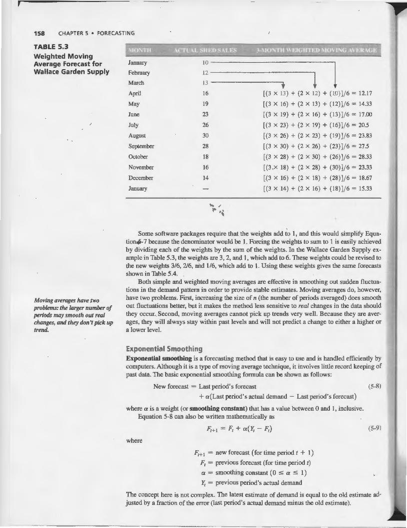
TABLE 5.3 Weighted Moving Average Forecast for Wallace Garden Supply

Moving averages have two problems: the larger number of periods may smooth out real changes, and they don't pick up trend.

January

February

March

April

May

June

July

August

September

October

November

December

January

10

12

13

16

19

23

26

30

28

18

16

14

1 l ((3 X 13 ) + (2 X 12) + (1:0) )/6 = 12.17

[(3 X 16) + (2 X 13) + (12))/6 = 14.33

[(3 X 19) + (2 X 16) + (13)) / 6 = 17.00

[(3 X 23) + (2 X 19) + (16) )/6 = 20.5

[(3 X 26) + (2 X 23) + (19)) / 6 = 23.83

[(3 X 30) + (2 X 26) + (23) )/6 = 27.5

[ (3 X 28) + (2 X 30) + (26) )/6 = 28.33

[(3 .X 18) + (2 X 28) + (30)] / 6 = 23.33

[(3 X 16) + (2 X 18) + (28) )/6 = 18.67

[(3 X 14) + (2 X 16) + (18)) / 6 = 15.33

Some software packages require that the weight-s add to 1, and this would simplify Equa­tio~-7 because the denominator would be 1. Forcing the weights to sum to 1 is easily achieved by dividing each of the weights by the sum of the weights. In the Wallace Garden Supply ex­ample in Table 5.3, the weights are 3, 2, and 1, which add to 6. These weights could be revised to the new weights 3/6, 2/6, and 1/6, which add to 1. Using these weights gives the same forecasts shown in Table 5.4. .

Both simple and weighted moving averages are effective in smoothing out sudden fluctua­tions in the demand pattern in order to provide stable estimates. Moving averages do, however, have two problems. First, increasing the size of n (the number of periods averaged) does smooth out fluctuations better, but it makes the method less sensitive to real changes in the data should they occur. Second, moving averages cannot pick up trends very well. Because they are aver­ages, they will always stay within past levels and will not predict a change to either a higher or a lower level.

Exponential Smoothing Exponential smoothing is a forecasting method that is easy to use and is handled efficiently by computers. Although it is a type of moving average technique, it involves little record keeping of past data. The basic exponential smoothing formula can be shown as follows:

New forecast = Last period's forecast (5-8)

+ a(Last period's actual demand - Last period's forecast)

where a is a weight (or smoothing constant) that has a value between 0 and 1, inclusive. Equation 5-8 can also be written mathematically as

where

F'r+l = Ft + a(Y; - Fr)

F1+ 1 = new forecast (for time period t + 1)

F1 = previous forecast (for time period t)

a = smoothing constant ( 0 :5 a :5 1)

Y, = previous period's actual demand

(5-9)

The concept here is not complex. The latest estimate of demand is equal to the old estimate ad­justed by a fraction of the error (last period's actual demand minus the old estimate).

the smoothing constant, a, alloWS managers to assign weight to recent data.

5.5 FORECASTING MODELS-RANDOM VARIATIONS ONLY 159

The smoothing constant, a, can be changed to give more weight to recent data when the value is high or more weight to past data when it is low. For example, when a = 0.5, it can be shown mathematically that the new forecast is based almost entirely on demand in the past three periods. When a = 0.1, the forecast places little weight on any single period, even the most re­cent, and it takes many periods (about 19) of historic values into account.*

For example, in January, a demand for 142 of a certain car model for February was predicted by a dealer. Actual February demand was 153 autos, so the forecast error was 153 - 142 = 9. Using a smoothing constant a = 0.20, the exponential smoothing forecast for March demand would be found by adding 20% of this error to the previous forecast of 142. Substituting into the formula, we obtain

Newforecast(forMarchdemand) = 142 + 0.2(153- 142)

. = 144.2 /"

Thus, the forecast for the demand for cars in March would be 144 after being rounded by the dealer.

Suppose that actual demand for the cars in March was 136. A forecast for the demand in April, using the exponential smoothing model with a constant of a = 0.20, cart be made:

New forecast (for April demand) = 144.2 + 0.2(136 - 144.2)

= 142.6, or 143 autos

GETTING STARTED The exponential smoothing approach is easy to use and has been applied successfully by banks, manufacturing companies, wholesalers, and other organizations. To develop a forecast with this method, a smoothing constant must be selected and a previous forecast must be known or assumed. If a company has been routinely using this method, there is no problem. However, if a company is just beginning to use the method, these issues must be addressed. ·

The appropriate value of the smoothing constant, a, can make the difference between an accurate forecast and an inaccurate forecast. In picking a value for the smoothing constant, the objective is to obtain the most accurate forecast. Several vi1tues of the smoothing constant may be tried, and the one with the lowest MAD could be selected. This is analogous to how weights are selected for a weighted moving average forecast. Some forecasting software will automati­cally select the best smoothing constant. QM for Windows will display the MAD that would be obtained with values of a ratlgif!¥. from 0 to 1 in increments of O.Ql.

When the exponential smoothing model is used for the first time, there is no prior forecast for the current time period to use in developing a forecast for the next time period. Therefore, a previous value for a forecast must be assumed. It is common practice to assume a forecast for time period 1, and to use this to develop a forecast for time period 2. The time period 2 forecast is then used to forecast time period 3, and this continues until the forecast for the current time period is found. Unless there is reason to assume another value, the forecast for time period 1 is assumed to be equal to the actual value in time period 1 (i.e.,_ the error is zero). The value of the forecast for time period 1 usually has very little impact on the value of forecasts many time periods into the future.

I

PORT OF BALTIMORE EXAMPLE Let us apply this concept with a trial-and-error testing of two values of a in an example. The port of Baltimore has unloaded large quantities of grain from ships during the past eight quarters. The port's operations manager wants to test the use of exponential smoothing to see how well the technique works in predicting tonnage unloaded. He assumes that the forecast of grain unloaded in the first quarter was 175 tons. Two values of a are examined: a= 0.10 and a= 0.50. Table 5.4 shows the detailed calculations for a= 0.10 only.

To evaluate the accuracy of each smoothing constant, we can compute the absolute devia­tions and MADs (see Table 5.5). Based on this analysis, a smoothing constant of a = 0.10 is preferred to a = 0.50 because its MAD is smaller.

•The term exponential smoothing is used because the weight of any one period's demand in a forecast decreases expo­nentially over time. See an advanced forecasting book for algebraic proof.

....... ----~--------160 CHAPTER 5 • FORECASTING

TABLE 5.4 Port of Baltimore Exponential Smoothing Forecasts for a = 0.10 and a = 0.50

TABLE 5.5 Absolute Deviations and MADs for the Port of Baltimore Example

2

3

4

5

6

7

8

9

2

3

4

5

6

7

8

180

168

159

175

190

205

180

182

180

168

159

175

190

205

180

182

?

\, • •

175

175.5 = 175.00 + 0.10(180- 75)

174.75 = 175.50 + 0.10(168- 75.50)

173.18 = 174.75 + 0.10(159- 174.75)

173.36 = 173.18 + 0.10(175- 173.18)

175.02 = 173.36 + 0.10(190- 173.36)

178.02 = 175.02 + 0.10(205- 175.02)

178.22 = 178.02 + 0.10(180- 178.02)

178.60 = 178.22 + 0.10(182- 178.22)

175 5 175

175.5 7.5 177.5

174.75 15.75 172.75

173.18 1.82 165.88

173.36 16.64 170.44

175.02 29.98 • 180.22

178.02 1.98 192.61

178.22 3.78 186.30

Sum of absolute deviations ...... 82.45

MAD= ~ I deviation I

= 10.31 n

Using Software for Forecasting Time Series

177.5

172.75

165.88

170.44

180.22

192.61

186.30

184.15

5

9.5

13.75

9.12

19.56

24.78

12.61

4.3

98.63

MAD= 12.33

The two software packages available with this book, Excel QM and QM for Windows, are very easy to use for forecasting. The previous examples will be solved using thesed

In using Excel QM with Excel 2013 for forecasting, from the Excel QM ribbon, select Alphabetical as shown in Program 5.1A. Then simply select whichever method you wish to use, and an initialization window opens to allow you to set the size of the problem. Program 5.1B shows this window for the Wallace Garden Supply weighted moving average example with the number of past periods and the number of periods in the weighted average already entered. Clicking OK results in the screen shown in Program 5.1C to appear allowing you to enter the data and the weights. Once all numbers are entered, the calculations are automatically performed as you see in Program 5.1C.

To use QM for Windows to forecast, under Modules select Forecasting. Then select New and Time Series Analysis as shown in Program 5.2A. This would be for all of the models

PROGRAM 5.1A Selecting the Forecasting Model in Wallace Garden Supply Problem

PROGRAM 5.18 Initializing Excel QM Spreadsheet for Wallace Garden Supply Problem

5.5 FORECASTING MODELS-RANDOM VARIATIONS ONLY 161

presented in this chapter. In the window that opens (Program 5.2B), specify the number of past periods of data. For the Port of Baltimore example, this is 8. Click OK and an input screen appears allowing you to enter the data and select the forecasting technique as shown in Program 5.2C. Based on the method you choose, other windows may open to allow you to specify the necessary parameters for that model. In this example, the exponential smoothing model is selected, so the smoothing constant must be specified. After entering the data, click Solve and the output shown in Program 5.2D appears. From this output screen, you can se­lect Window to see additional information such as the details of the calculations and a graph of the time series and the forecasts .

( INSERT PAGE LAYOUT FORMULAS DATA REVIEW VIEW Excel QM

Mtnus

I P33 ~--i

1 2 3 4

A

linear. Integer Ill MQo,d Integer l'n>gramming

Marlcov Chains

Material Requirements Planning

Ndwork Analysis

Ne.twotfc Analysis as LP

Project Managemert

Quality Control

Simulation

Statistics {mean, var, ~ Normal Dist)

T IaRSpOrtation

Wailing Unes

Color

ing

~ ~preferenc< ~Default colol5

Tr~endfxponential Smoothing Reg . Analy5is

Multiple R .

Multiplicativi Seasonal Model

. -+-­

~~~-.r-~~-----~

();splay OM~~~

OisplayQMMO<Il'IS"~ t- t ---=--· -·- - ~-...__Oisplay __ AI_ Mod_ ell; ______ __.rc_J _ _

Spreadshe:et . . Enter a title.

NuMet 0( ~Past) periods ol diD 0 .~ MIMe for pertod l '-'-Ped..;.;....;.od.:.._ __ __,l (Usr A for A. B, C.- or a for~ b, < - l

Nulllbu Of periods to~

Enter the number of periods to be averaged.

162 CHAPTER 5 • FORECASTING

PROGRAM 5.1 C

Excel QM Output for Wallace Garden Supply Problem

PROGRAM 5.2A Selecting Time-Series Analysis in QM for Windows in the Forecasting Module

PROGRAM 5.28

Entering Data for Port of Baltimore Example in QM for Windows

PROGRAM 5.2C

Selecting the Model and Entering Data for Port of Baltimore Example in QM for Windows

A B _I;_, Enter the demand data and the weights. The\... 1 Wallace Garden Sup~ calculations will automatically be performed. 2

8 Period Demand W"eiQhts uared Abs Pet Err 9 Period 1 10 1 10 Period 2 12 2 11 Period 3 13 .3 12 Period 4 16 12.16667 3 833333 3 833333 14.69444 13 Period 5 19 14.33333 4 666667 • 666667 21.77778 14 Penod6 z 11 6 6 36 15 Penod 7 2li 20.5 5.5 5-5 :11.:25 16 Penod 8 30 23 83333 6166607 6.166667 38.02718 17 Period 9 2ll

I 18 Period 10 11 The measures of accuracy are shown here. 19 Period 11 1 " 20 Period 12 14 1 4.666667 21.77778 33.33%

49 323.3333 254.611%

,.,-------rln the Forecasting module, click"., New and Time-Series Analysis.

~ l•ast Squares - Simp

~~Projector

§. &ror Analysis

r. Past period 1. Past period 2. Past period 3 .... r a, b. c, d.e ... . r A. B. C. D. E .. . r 1. 2. 3. 4. 5 ... . r January, February, March, Apri •...

I Click here to set start month ::!]

PROGRAM 5.20

Output for Port of Baltimore Example in QM for Windows

5.6 FORECASTING MODELS-TREND AND RANDOM VARIATIONS 163

ll 51< tdit y.,.. Module Fopmt !ools I Wtndow !f<lp

Dflloo liiilllt j 'tlft j~J~I "' c7~Add"f I t t" J . He I IOna OU pu IS ~ Ana •

9.7!· 1 [il Edito.t \ available under Window. Method a

begr,; in period 2. I EJ<pOnenl;.j Smoothilg ~ Fo<ecasting Results I

' . ~~ .... ,.. l Emu< as a function ol alpha ~ ~. .I

~ Cor<roi [T<ading Signal] ( P<HI ol&llllllllfe Summaoy

MNsllre ~G<aph

I Em>rMa"""""' Bias {Mean fmlll 1.069 ~The measures of MAD {Mean Absmute o.Malion) 10.868 accuracy are shown here. MSE (Mean Sql- fm11l 207.24

Standard Em>r (denorrFn-.2;o5) 17.033

MAPE .{MeanAI>solut• P<lmlflt Em>r) 5.999% ~The forecast for next Forecast

period is here. k nexl period 180.748

5.6 Forecasting Models-Trend and Random Variations

TWo smoothing constants are used. '

Estimate or assume initial values for Ft and'!;_

If there is trend present in a time series, the forecasting model must account for this and cannot simply average past values. Two very common techniques will be presented here. The first is ex­ponential smoothing with trend, and the second is called trend projection or simply a trend line.

Exponential Smoothing with Trend An extension of the exponential smoothing model that will explicitly adjust for trend is called the exponential smoothing with trend m~del. The idea is to develop an exponential smooth­ing forecast and then adjust this for trend. Two smoothing constants, a and {3, are used in this model, and both of these values must be between 0 and 1. The level of the forecast is adjusted by multiplying the first smoothing constant, a, by the most recent forecast error and adding it to the previous forecast. The trend is adjusted by multiplying the second smoothing constant, {3, by the most recent error or excess amount in the trend. A higher value gives more weight to recent observations and thus respo,~s more quickly to changes in the patterns.

As with simple expo'neg~ smoothing, the first time a forecast is developed, a previ­ous forecast (F1) must be given or estimated. If none is available, often the initial forecast is assumed to be perfect. In addition, a previous trend ('z;) must be given or estimated. This is often estimated using other past data, if available, or by using subjective means, or by calcu­lating the increase (or decrease) observed during the first few time periods of the data avail­able. Without such an estimate available, the trend is sometimes assumed to be 0 initially, although this may lead to poor forecasts if the trend is large and {3 is small. Once these initial conditions have been set, the exponential smoothing forecast including trend (FITr) is devel­oped using three stel?s:

Step 1. Compute the smoothed fore~ast (F1+1) for time period t + 1 using thy equation

Smoothed forecast = Previous forecast including trend + a(Last error)

F1+ 1 = F!Tr + a( ft - FITr) (S-10)

Step 2. Update the trend (Tr+ 1) using the equation

Smoothed trend = Previous trend + {3(Error or excess in trend)

'Fr+t = Tr + f3(Ft+l - FITr) (5-11)

Step 3. Calculate the trend-adjusted exponential smoothing forecast (FITr+t) using the equation

Foreca~tincluding trend (FITr+I) = Smoothed forecast (F1+t) + Smoothed trend (Tr+J)

FITr+ 1 = Ft+ 1 + 'Tr+ 1 (S-12)

164 CHAPTER 5 • FORECASTING

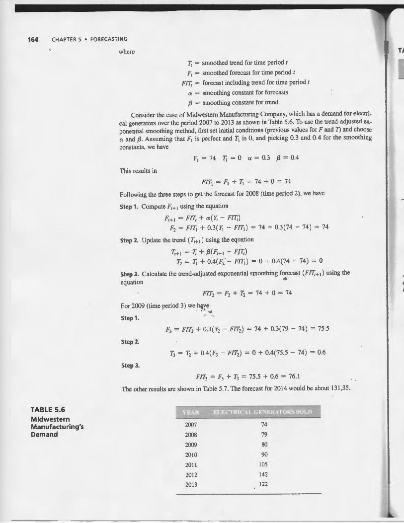
TABLE 5.6 Midwestern Manufacturing's Demand

where

fe = smoothed trend for time period t

F1

= smoothed forecast for time period t

Fife = forecast including trend for time period t

a = smoothing constant for forecasts

{3 = smoothing constant for trend

Consider the case of Midwestern Manufacturing Company, which has a demand for electri­cal generators over the period 2007 to 2013 as shown in Table 5.6. To use the trend-adjusted ex­ponential smoothing method, first set initial conditions (previous values for F and T) and choose a and {3 . Assuming that F1 is perfect and 7J is 0, and picking 0.3 and 0.4 for the smoothing constants, we have

F1 = 74 T1 = 0 a = 0.3 {3 = 0.4

This results in

F!Tt = F1 + Tt = 74 + 0 = 74

Following the three steps to get the forecast for 2008 (time period 2), we have

Step 1. Compute Fr+ l using the equation

Fr+ l = Fife+ a(Y;- Fife)

F2 = FIT1 + 0.3(lj - FIT1) = 74 + 0.3(74- 74) = 74

Step 2. Update the trend ( fe+ 1) using the equation

fe+t = fe + f3(Fr+ l - F,lfe)

Ti = Tt + 0.4(F2 - F!Tt) = 0 + 0.4(74- 74) = 0

Step 3. Calculate the trend-adjusted exponential smoothing forecast (Fife+ 1) using the .. equation

FIT2 = F2 + T2 = 74 + 0 = 74

For 2009 (time period 3) we h~ve • j ....

Step 1. "

F3 = FIT2 + 0.3(Y2 - FIT2) = 74 + 0.3(79 - 74) = 75 .5

Step 2.

T3 = T2 + OA(F3 - FIT2) = 0 + 0.4(75.5 - 74) = 0.6

Step 3.

FIT:J = F3 + T3 = 75.5 + 0.6 = 76.1

The other results are shown in Table 5. 7. The forecast for 2014 would be about 131 .35.

2007 74

2008 79

2009 80

2010 90

2011 105

2012 142

2013 122

T~

}

5.6 FORECASTING MODELS-TREND AND RANDOM VARIATIONS 165

TABLE 5.7 Midwestern Manufacturing Exponential Smoothing with Trend Forecasts

74 74 0 74

2 79 74 = 74 + 0.3(74- 74) 0 = 0 + 0.4(74 - 74) 74 = 74 + 0

3 80 75.5 = 74 + 0.3(79 - 74) 0.6 = 0 + 0.4(75.5 - 74) 76.1 = 75.5 + 0.6

4 90

5 105

6 142

7 122

8

A trend line is a regression equation with time as the independent variable.

PROGRAM 5.3

77.270 1.068 78.338 = 77.270 + 1.068 = 76. I + 0.3(80 - 76.1) = 0.6 + 0.4(77.27 - 76.1)

81.837 2.468 84.305 = 81.837 + 2.468 = 78.338 + 0.3(90 - 78.338) = 1.068 + 0.4(81.837 - 78.338)

90.514 4.952 95.466 = 90.514 + 4.952 = 84.305 + 0.3 ( 105 - 84.305) = 2.468 + 0.4(90.514 - 84.305)

109.426 10.536 119.962 = 109.426 + 10.536 = 95.466 + 0.3 ( 142 - 95.466) = 4.952 + 0.4( 109.426 - 95.466)

120.573 10.780 131.353 = 120.573 + 10.780 = 119.962 + 0.3(122- 119.962) = 10.536 + 0.4(120.573 - 119.962)

To have Excel QM perform the calculations in Excel2013, from the Excel QM ribbon, select the alphabetical list of techniques and choose Forecasting and then Trend Adjusted Exponential Smoothing . After specifying the number of past observations, enter the data and the values for a and {3 as shown in Program 5.3.

Trend Projections Another method for forecasting time series with trend is called trend projection. This tech­nique fits a trend line to a series of historical data points and then projects the line into the future for medium- to long-range forecasts. There are sevei1! mathematical trend equations that can.be developed (e.g., exponential and quadratic), but in this section we look at linear (straight line) trends only. A trend line is simply a linear regression equation in which the independent

' t- ..t , ""

Output from Excel QM in Excel 2013 for Trend Adjusted Exponential Smoothing Example

------------------------------- ------- ------------

166 CHAPTER 5 • FORECASTING

PROGRAM 5.4

Output from Excel QM in Excel 2013 for Trend Line Example

variable (X) is the time period. The first time period will be time period 1. The second thne period will be time period 2, and so forth. The last time period will be time period n. The fol11J. of this is

where

Y = predicted value

b0 = intercept

b1 = slope of the line

X= time period (i.e., X= 1, 2, 3, ... , n)

The least squares regression method may be applied to find the coefficients that minimize the sum of the squared errors, thereby also minimizing the mean squared error (MSE). Chapter 4 provides detailed explanation of least squares regression and formulas to calculate the coefficients by hand. In this section, we use computer software to perform the calculations.

Let us consider the case of Midwestern Manufacturing's demand for generators that was presented in Table 5.6. A trend line can be used to predict demand (f) based on the time period using a regression equation. For the first time period, which was 2007, we let X = 1. For 2008, we let X = 2, and so forth. Using computer software to develop a regression equation as we did in Chapter 4, we get the following equation:

Y = 56.71 + 10.54X

To project demand in 2014, we first denote the year 2014 in our new coding system as X= 8:

(sales in 2014) = 56.71 + 10.54(8)

= 141.03, or 141 generators

We can estimate demand for 2015 by inserting X = 9 in the same equation:

(sales in 2015) = 56.71 + 10.lf(9)

= 151.57, or 152 generators

Program 5.4 provides output from Excel QM in Exce12013. To run this model, from the Excel QM ribbon, select Alphabftical to see the techniques. Then select Forecasting and Regression/ Trend Analysis. When the rnpht window opens, enter the number of past observations (7), and the spreadsheet is initialized allowing you to input the seven Y values and the seven X values as shown in Program 5.4.

s

el ,; td as

pROGRAM 5.5 output from QM for Windows in Excel 2013 tor Trend Line Example

FIGURE 5.4 Generator Demand and Projections for Next Three Years Based on Trend Line

5.7 ADJUSTING FOR SEASONAL VARIATIONS 167

,("', .,., I

( Forecasts for future time };; Measure Forecast periods are shown here. · 1"---

Error MeastRs 8 ------ 141 Bias (Mean Error} 0 9 151 .536 MAD (MeanAbsolt.te Devialion) 8.582 10 162.071 MSE (Mean Squa'ed Error) 110.403 11 172.607 Staodarcl Error (deoom--n-2,5) 12.432 12 183.143 MAPE (MeanAbsok1e Percent 8.224% 13 193.679 Regression lite 14 204214

) -56.71-4 15 214.75 !

+ 10.536~Tme(x). 16 225.286 Statistics

----- I The trend line is \ 235.822 Cooefafion coellicient

-:----!\.. shown over two lines.) 246.357

Coefficient at detem1ination (r'2) 256.893 20 267.429

I 21 1 277.964

180

160

140

" Trend Line Y = 56.71 + 10.54X •••• x

. \ .. -~-----~\/ .~ ~ "C 120 c: ttl E

•••• •• • • Projected demand for •• • • • • • next 3 years is shown on

•••• ,.·· • ~ the trend line. Q) 100 0

~ 80 Q) c: Q)

60 (!)

40

20

00

., . ............... "' . .. ·· . . ..·· ... •

2 3 4

.1

5 6 7 8 9 10 11

Time Period

This problem could also be solved using QM for Windows. To do this, select the Forecast­ing module, and then enter a new problem by selecting New- Time Series Analysis. When the next window opens, enter the number of observations (7) and press OK. Enter the values (Y) for the seven past observations when the input window opens. It is not necessary-to enter the values for X (1, 2, 3, ... , 7) because QM for Windows will automatically use' these numbers. Then click Solve to see the results shown in Program 5.5.

Figure 5.4 provides a scatter diagram and a trend line for this data. The projected demand in each of the next three years is also shown on the trend line.

5. 7 Adjusting for Seasonal Variations

Time-series forecasting such as that in the example of Midwestern Manufacturing involves looking at the trend of data over a series of time observations. Sometimes, however, recurring variations at certain seasons of the year make a seasonal adjustment in the trend line forecast necessary. Demand for coal and fuel oil, for example, usually peaks during cold winter months.

168 CHAPTER 5 • FORECASTING

An average season has an index of 1.

TABLE 5.8

Answering Machine Sales and Seasonal Indices

Demand for golf clubs or suntan lotion may be highest in summer. Analyzing data in monthly or quarterly terms usually makes it easy to spot seasonal patterns. A seasonal index is often usect in multiplicative time-series forecasting models to make an adjustment in the forecast when a seasonal component exists. An alternative is to use an additive model such as a regression model that will be introduced in a later section.

Seasonal Indices A seasonal index indicates how a particular season (e.g., month or quarter) compares with an average season. An index of 1 for a season would indicate that the season is average. If the index is higher than 1, the values of the time series in that season tend to be higher than average. If the index is lower than 1, the values of the time series in that season tend to be lower than average.

Seasonal indices are used with multiplicative forecasting models in two ways. First, each observation in a time series are divided by the appropriate seasonal index to remove the impact of seasonality. The resulting values are called deseasonalized data. Using these deseasonalized val­ues, forecasts for future values can be developed using a variety of forecasting techniques. Once the forecasts of future deseasonalized values have been developed, they are multiplied by the seasonal indices to develop the final forecasts, which now include variations due to seasonality.

There are two ways to compute seasonal indices. The first method, based on an overall average, is easy and may be used when there is no trend present in the data. The second method, based on a centered-moving-average approach, is more difficult but it must be used when there is trend present.

Calculating Seasonal Indices with No Trend When no trend is present, the index can be found by dividing the average value for a particular season by the average of all the data. Thus, an index of 1 means the season is average. For ex­ample, if the average sales in January were 120 and the average sales in all months were 200, . the seasonal index for January would b,e 120/ 200 = 0.60, so January is below average. The next example illustrates how to compute seasonal indices from historical data and to use these in forecasting future values.

Monthly sales of one brand of telephone answering ti)IJ.Chine at Eichler Supplies are shown in Table 5.8, for the two most recent years. The average demand in each month is computed, and these values are divided by the overall average (94) to find the seasonal index for each month. We then use the seasonal indices from Table 5.8 to adjust future forecasts. For example, suppose we expected the third year.,.. annual demand for answering machines to be 1,200 units, which is

. ' ...l

January 80

February 85

March 80

April 110

May 115

June 120

July 100

August 110

September 85

October 75

November 85

December 80

,

100

75

90

90

131

110

110

90

95

85

75

80

90

80

85

100

123

115

105

100

90

80

80

80

94

94

94

94

94

94

94

94

94

0.957

0.851

0.904

1.064

1.309

1.223

1.117

1.064

0.957

94 0.851

94 0.851

94 0.851

Total average demand = ~ \

1,128 ;:::::::--'" b Average 2 year de'mand • Average monthly demand= = 94 Seasonal index = __ _::___:__ ___ _

12 months Average monthly demand

Centered moving averages are used to compute seasonal indices when there is trend.

TABLE 5.9

Quarterly Sales ($1,000,000s) for Turner Industries

5.7 ADJUSTING FOR SEASONAL VARIATIONS 169

100 per month. We would not forecast each month to have a demand of 100, but we would adjust these based on the seasonal indices as follows:

Jan. 1,200 12 X 0.957 = 96 July

1 '~~ X 1.117 = 112

Feb. 1,200

Aug. 1'200

X 1 064 = 106 -- X 0851 = 85 12 . 12 .

Mar. 1,200

Sept. 1'200

X 0 957 = 96 -- X 0904 = 90 12 . 12 .

Apr. 1,200

Oct. 1,200 12 X 1.064 = 106 -- X 0.851 = 85

12

May 1200 -t- X 1.309 = 131 Nov.

1,200 }2 X 0.851 = 85

June 1 '~~0 X 1.223 = 122 Dec.

1•200

X 0 851 = 85 12 .

Calculating Seasonal Indices with Trend When both trend and seasonal components are present in a time series, a change from one month to the next could be due to a trend, to a seasonal variation, or simply to random fluctuations . To help with this problem, the seasonal indices should be computed using a centered moving average (CMA) approach whenever trend is present. Using this approach prevents a variation due to trend from being incorrectly interpreted as a variation due to the season. Consider the following example.

Quarterly sales figures for Turner Industries are shown in Table 5.9. Notice that there is a definite trend as the total is increasing each year, and there is an increase for each quarter from one year to the next as well. The seasonal component is obvious as there is a definite drop from the fourth quarter of one year to the first quarter of the next. A similar pattern is observed in comparing the third quarters to the fourth quarters immediately following.

If a seasonal index for quarter 1 were computed using the o~rall average, the index would be too lo~ and misleading, since this quarter has less trend than any of the others in the sample. If the first quarter of year 1 were omitted and replaced by the first quarter of year 4 (if it were available), the average for quarte\) (and consequently the seasonal index for quarter 1) would be considerably higher. To derive ~~curate seasonal index, we should use a CMA.

Consider quarter 3 of year 1 for the Turner Industries example. The actual sales in that quarter were 150. To determine the magnitude of the seasonal variation, we should compare this with an average quarter centered at that time period. Thus, we should have a total of four quar­ters (1 year of data) with an equal number of quarters before and after quarter 3 so the trend is averaged out. Thus, we need 1.5 quarters before quarter 3 and 1.5 quarters after it. To obtain the CMA, we take quarters 2, 3, and 4 of year 1, plus one-half of quarter 1 for year 1 and one-half of quarter 1 for year 2. The average will be

( 0.5(108) + 125 + 150 + 141 + 0.5(116) , .

CMA quarter 3 of year 1) = 4

= 13~.00

We compare the actual sales in this quarter to the CMA and we have the following seasonal ratio:

Seasonal ratio = Sales in quarter 3 150

1.136 =--= CMA 132.00

108 116 123 115.67

2 125 134 142 133.67

3 150 159 168 159.00

4 141 152 165 152.67

Average 131.00 140.25 149.50 140.25

170 CHAPTER 5 • FORECASTING

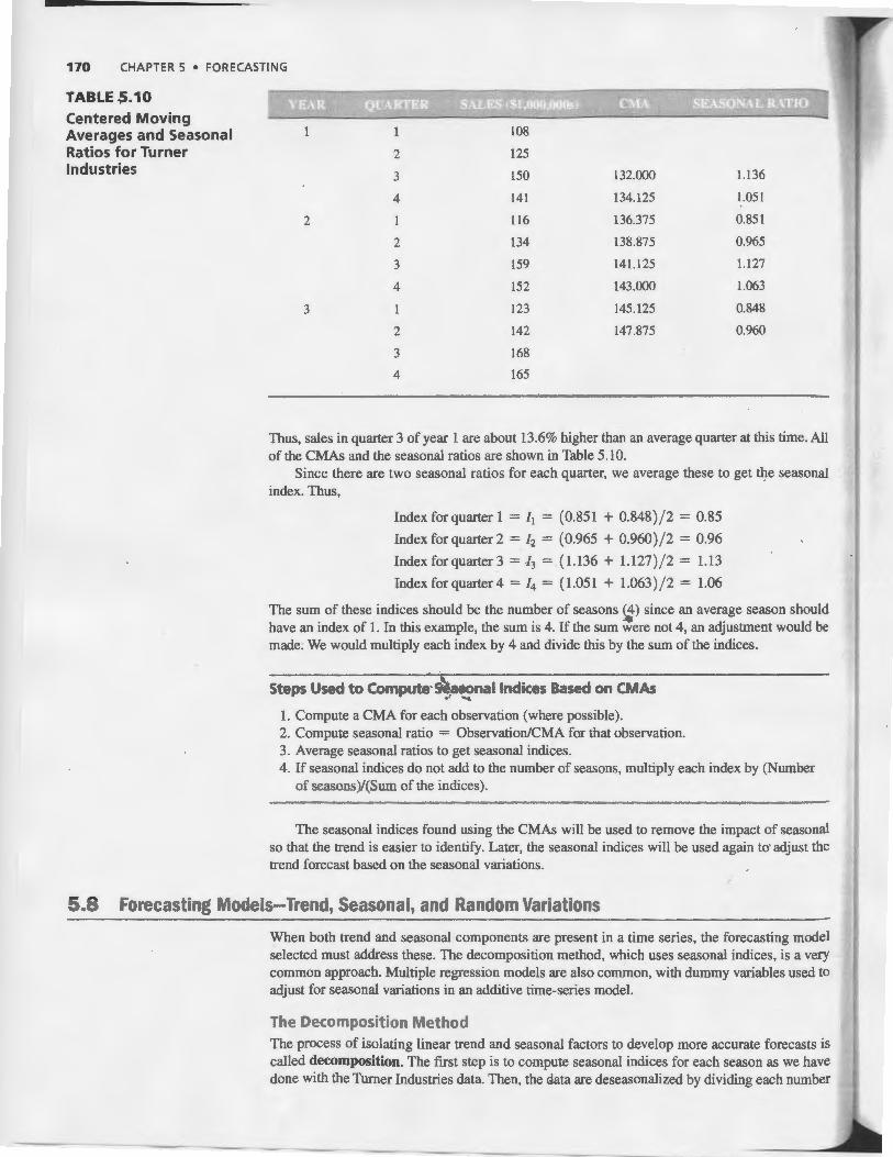
TABLE-:;.10

Centered Moving Averages and Seasonal Ratios for Turner Industries

125

3 150 132.000 1.136

4 141 134.125 1.051

2 116 136.375 0.851

2 134 138.875 0.965

3 159 141.125 1.127

4 152 143.000 1.063

3 123 145.125 0.848

2 142 147.875 0.960

3 168

4 165

Thus, sales in quarter 3 of year 1 are about 13.6% higher than an average quarter at this time. All of the CMAs and the seasonal ratios are shown in Table 5.10.

Since there are two seasonal ratios for each quarter, we average these to get the seasonal index. Thus,

Index for quarter 1 =It = (0.851 + 0.848) / 2 = 0.85

Index for quarter 2 = h = (0.965 + 0.960) / 2 = 0.96

Indexforquarter3 = h = (1.136 + 1.127) / 2 = 1.13

Index for quarter 4 = /4 = ( 1.051 + 1.063) / 2 = 1.06

The sum of these indices should be the number of seasons (4) since an average season should have an index of 1. In this example, the sum is 4. If the sum :ere not 4, an adjustment would be made: We would multiply each index by 4 and divide this by the sum of the indices.

Steps Used to Compute· S~aeonallndices Based on CMAs

1. Compute a CMA for each observation (where possible). 2. Compute seasonal ratio = Observation/CMA for that observation. 3. Average seasonal ratios to get seasonal indices. 4. If seasonal indices do not add to the number of seasons, multiply each index by (Number

of seasons)/(Sum of the indices).

The seasonal indices found using the CMAs will be used to remove the impact of seasonal so that the trend is easier to identify. Later, the seasonal indices will be used again to· adjust the trend forecast based on the seasonal variations.

5.8 Forecasting Models-Trend, Seasonal, and Random Variations

When both trend and seasonal components are present in a time series, the forecasting model selected must address these. The decomposition method, which uses seasonal indices, is a very -common approach. Multiple regression models are also common, with dummy variables used to adjust for seasonal variations in an additive time-series model.

The Decomposition Method The process of isolating linear trend and seasonal factors to develop more accurate forecasts is called decomposition. The first step is to compute seasonal indices for each season as we have done with the Turner Industries data. Then, the data are deseasonalized by dividing each number

TABLE 5.11 peseasonalized Data for Turner Industries

FIGURE 5.5

Scatterplot of Turner Industries's Original Sales Data and Deseasonalized Data

5.8 FORECASTING MODEL5-TREND, SEASONAL, AND RANDOM VARIATIONS 171

108 0.85 127.059

125 0.96 . 130.208

150 1.13 132.743

141 1.06 133.019

116 0.85 136.471

134 0.96 139.583

159 1.13 140.708

152 1.06 143.396

123 0.85 144.706

142 0.96 147.917

168 1.13 148.673

165 1.06 155.660

by its seasonal index, as shown in Table 5.11. Figure 5.5 provides a graph of the original data as well as a graph of the deseasonalized data. Notice how smooth the deseasonalized data is.

A trend line is then found using the deseasonalized data. Using computer software with this data, we have*

The trend equation is

where

. ' • ' .. -.A .,. .....

200

150 • • X X X

X X

• • :g ~ 100

50

bl = 2.34

b0 = 124.78

• Y = 124.78 + 2.34X

X= time

• • X X

X X •

•

X •

• Sales Data

• • X

X

~

x Deseasonalized Sales Data

0 0 2 3 4 5 6 7 8 9 10 11 12 13

Time Period (Quarters)

*If you do the calculations by hand, the numbers may differ slightly from these due to rounding.

172 CHAPTER 5 • FORECASTING

TABLE 5.12 Turner Industry Forecasts for Four Quarters of Year 4 '

FIGURE 5.6

2

3

4

Scatterplot of Turner Industries Original Sales Data and Deseasonalized Data with Unadjusted and Adjusted Forecasts

14

15

16

157.54

159.88

162.22

0.96

1.13

1.06

151.24

180.66

171.95

This equation is used to develop the forecast based on trend, and the result is multiplied by the appropriate seasonal index to make a seasonal adjustment. For the Turner Industries data, the forecast for the first quarter of year 4 (time period X = 13 and seasonal index It = 0.85) would be found as follows:

Y = 124.78 + 2.34X

= 124.78 + 2.34( 13)

= 155.2 (forecast before adjustment for seasonality)

We multiply this by the seasonal index for quarter l and we get

Y X It = 155.2 X 0.85 = 131.92

Using the same procedure, we find the forecasts for quarters 2, 3, and 4 of the next year. Table 5.12 shows the unadjusted forecast based on the trend line, for each of the four quarters of year 4. The last column of this table gives the final forecasts that were found by multiplying each trend forecast by the appropriate seasonal index. A scatter diagram showing the original data and the deseasonalized data as well as the unadjusted forecast and the final forecast for these next four quarters is provided in Figure 5.6.

Steps to Develop a Forecast Using the Decomposit on Method

1. Compute seasonal indices using CMAs. 2. Deseasonalize the data by dividing each number by its seasonal index. 3. Find the equation of a ~e~ line using the deseasonalized data. 4. Forecast for future periods 11sing the trend line. 5. Multiply the trend line forecast by the appropriate seasonal index.

200

• • 150

.............. •

• •

gJ bii 100

•

• Sales Data A Deseasonalized Sales Data

• Unadjusted Trend Forecast 50 • Forecast Adjusted for Season

0 0 2 3 4 5 6 7 8 ,g 10 11 12 13 14 15 16

Time Period (Quarters)

PROGRAM 5.6A QM for Windows Input Screen for Turner Industries Example

PROGRAM 5.68 QM for Windows Output Screen for Turner Industries Example

5.8 FORECASTING MODEL5-TREND, SEASONAL, AND RANDOM VARIATIONS 173

Most forecasting software, including Excel QM and QM for Windows, includes the decompo­sition method as one of the available techniques. This will automatically compute the CMAs, deseasonalize the data, develop the trend line, make the forecast using the trend equation, and adjust the final forecast for seasonality.

Software for Decomposition Program 5.6A shows the QM for Windows input screen that appears after selecting the Forecast­ing Module, selecting New-Time Series, and specifying 12 past observations. The multiplicative decomposition method is selected, and you can see the inputs that are used for this problem. When this is solved, the output screen in Program 5.6B appears. Additional output is available by selecting details or graph from the Windows drop-down menu (not shown in Program 5.6B) that appears after the problem is solved. The forecasts are slightly different from the ones shown in Table 5.12 due to round-off error.

Excel QM can be used in Excel2013 for this problem also. From the QM Ribbon, select the menus By Chapter and select Chapter 5-Forecasting-Decomposition. Specify there are 12 past observations, 4 seasons, and use a centered moving average.

Specify Centered Moving

0verage approach Select Rescale:

...._set average to 1 )

152 123 142 168 165

Specify the number of seasons ,_J4 for quarterly data)

! select Multiplicative Decomposition"\ \,from the drop-d~n menu. /

Input the data

se.w IM~Deo~ticn{seMonal] 31 c r I 4 The final forecast is obtained by multiplying

' - - • · the trend (unadjusted) forecast by the efael

seasonal indices (factors).

13 131.81 0.001 14 0.963 151.687 0905 15 159.937 1131 11!0.959

1.7 16 162.281 1.057 171.535 1.844 17 164.625 0.849 139.769

0.595% 18 166.968 0963 160 71 19 169.312 1.131 191566 20 171.655 1.057 81.444 21 1n.999 0.849 147.728

The trend line is shown 22 176.342 0963 169 733 23 178.686 1.131 202.1n

here over two lines. 24 181.03 1.057 191.353 25 183.373 0.849 155.686 26 185.717 0963 178.756

174 CHAPTER 5 • FORECASTING

Multiple regression can be used to develop an additive decomposition model.

PROGRAM 5.7A Excel QM Multiple Regression Initialization Screen for Turner Industries

Usang Regression with Trend and Seasonal Components Multiple regression may be used to forecast with both trend and seasonal components present in a time series. One independent variable is time, and other independent variables are dummy variables to indicate the season. If we forecast quarterly data, there are four categories (quarters) so we would use three dummy variables. The basic model is an additive decomposition model and is expressed as follows:

where

X1 = time period

x2 = 1 if quarter 2

= 0 otherwise

x3 = 1 if quarter 3

= 0 otherwise

x4 = 1 if quarter 4

= 0 otherwise

If x 2 = x 3 = x4 = o. then the quarter would be quarter 1. It is an arbitrary choice as to which of the quarters would not have a specific dummy variable associated with it. The forecasts will be the same regardless of which quarter does not have a specific dummy variable.

Using Excel QM in Excel2013 to develop the regression model, from the Excel QM ribbon, we select the menu for Chapter 5-Forecasting, and then choose the Multiple Regression method. The input screen in Program 5.7A appears, and the number of observations (12) and the number of independent variables ( 4) are entered. An initialized spreadsheet appears and the values for all the variables are entered in columns B through F as shown in Program 5.7B. Once this has been done, the regression coefficients appear. The regression equation (with rounded coefficients) is

A

Y = 104.1 + 2.3Xl + 15.7X2 + 38.7X3 + 30.1X4

If this is used to forecast sales in the first quarter of the next year, we get

y = 104.1 + 2.3(13) + 15.7(0) + 38.7(0) + 30.1(0) = 134

For quarter 2 of the aeJUtyear, we get

y = l04.1 + 2.3(14) + 15.7(1) + 38.7(0) + 30.1(0) = 152

Notice these are not the same values we obtained using the multiplicative decomposition method. We could compare the MAD or MSE for each method and choose the one that is better.

s~ Initialization

Td:le: [Tum .. lndustries

Number of {past) periods of rdata ___ 11_2---,j ffi Nam• far pffiod I Ptriod I ""' ttJst!A for A. 8, C .•• or a for a, b, c .• .t

Nulnber of indi!Pm<lerd: varlabl•sOCI CJ ffi Namefoocs j '--x ____ _,j

Help

jl

Enter the number of past period of data .

Enter the number of independent variables.

5.9 M ONITORING AND CONTROLLING FORECASTS 175

Forecasting at Disney World

W hen the Disney chairman receives a daily report f rom his main theme parks in Orlando, Florida, the report contains only two num­bers: the forecast of yesterday's attendance at the parks (Magic Kingdom, Epcot, Fort Wilderness, Hollywood Studios (formerly MGM Studios). Animal Kingdom, Typhoon Lagoon, and Blizzard Beach) and the actual attendance. An error close to zero (using MAPE as the measure) is expected. The chairman takes his forecasts very seriously.

With 20% of Disney World 's customers coming from outside the United States, its econometric model includes such variables as consumer confidence and the gross domestic product of seven countries. Disney also surveys one million people each year to exam ine their future travel plans and their experiences at the parks. Th is helps forecast not only attendance, but behavior at each ride (how long people will wait and how many times they w ill ride). Inputs to the monthly forecasting model include airline specials, speeches by the chair of the Federal reserve, and Wall Street trends. Disney even monitors 3,000 school districts inside and outside the United States for holiday/vacation schedules.

The forecasting team at Disney World doesn 't just do a daily prediction, however, and the chairman is not its only customer. It also provides daily, weekly, monthly, annual , and 5-year forecasts to the labor management, maintenance, operations, finance, and park scheduling departments. It uses judgmental models, econo­metric models, moving average models, and regression analysis. The team's annual forecast of total volume, conducted in 1999 for the year 2000, resulted in a MAPE of 0.

Source: Based on J. Newkirk and M. Haskell. "Forecasting in the Service Sector," presentation at the 12th Annual Meeting of the Production and Operations Management Society. April I, 2001, Orlando, FL.

PROGRAM 5.78

Excel QM Multiple Regression Output Screen for Turner Industries

A B C D E F

1 l Turner Industries 2 3 Forecasting Mi( Enter the values of ) : ~ .._ ... ,. ... !Iii! ,~ Y and X1- X4 as shown.

6 / -7 Data

., 8 y XI /X 2 X3 X4 9 Period 1 , ~- T • .· J -· ·

t ::v 10 Period 2 ···.· Z: . 0\ c'l····'* ·"- '"'"a ·.,•. 11 Pe<iod 3 .3 .. I. -~1 .l .. 12 Period • . .,

The regression coefficient0 13 Period5 14 Period 6 ._are sh~wn here. ./ 15 Period 7

~~eriod8 1Sf .... :• 0 1

~Enter the values of the variab les -~· ll .

to obtain any forecast . -:f . '. A' ·' t ·

21

10..1~~ 22 Coe4icienls 38.708 30.063 231

-24 f 25 FOfecasl 1~. 167 13. • 0 • J

•

5.9 Monitoring and Controlling Forecasts

A tracking signal measures how Well predictions fit actual data.

After a forecast has been completed, it is important that it not be forgotten. No manager wants to be reminded when his or her forecast is horribly inaccurate, but a firm needs to determine why the actual demand (or whatever variable is being examined) differed significantly from that projected.*

One way to monitor forecasts to ensure that they are performing well is to employ a tracking signal. A tracking signal is a measurement of how well the forecast is predicting actual values. As forecasts are updated every week, month, or quarter, the newly available demand data are compared to the forecast values.

' If the forecaster is accurate, he or she usually makes sure that everyone is aware of his or her talents. Very seldom does one read articles in Fortune, Forbes, or the Wall Street Journal, however, about money managers who are consistently off by 25%' in their stock market forecasts . •

176 CHAPTER 5 • FORECASTING

Setting tracking limits is a matter of setting reasonable values for upper and lower limits.

FIGURE 5.7 Plot of Tracking Signals

The tracking signal is computed as the running sum of the forecast errors (RSFE) divided by the mean absolute deviation:

where

as seen earlier in Equation 5-1 .

RSFE Tracking signal = MAD

L (forecast error)

MAD

L I forecast error I MAD = _____; ____ ...:... n

(5-13)

Positive tracking signals indicate that demand is greater than the forecast. Negative signals mean that demand is less than forecast. A good tracking signal-that is, one with a low RSFE-has about as much positive error as it has negative error. In other words, small deviations are okay, but the posi­tive and negative deviations should balance so that the tracking signal centers closely around zero.

When tracking signals are calculated, they are compared with predetermined control limits. When a tracking signal exceeds an upper or lower limit, a signal is tripped. This means that there is a problem with the forecasting method, and management may want to reevaluate the way it forecasts demand. Figure 5.7 shows the graph of a tracking signal that is exceeding the range of acceptable variation. If the model being used is exponential smoothing, perhaps the smoothing constant needs to be readjusted.

How do fmns decide what the upper and lower tracking limits should be? There is no single answer, but they try to find reasonable values-in other words, limits not so low as to be trig- · gered with every small forecast error and not so high as to allow bad forecasts to be regularly overlooked. George Plossl and Oliver Wight, two inventory control experts, suggested using maximums of ± 4 MADs for high-volume stock items and ± 8 MADs for lower-volume items.*

Other forecasters suggest slightly lower ranges. One MAD is equivalent to approximately 0.8 standard deviation, so that ± 2 MADs = 1.6~tandard deviations, ± 3 MADs = 2.4 stan­dard deviations, and ± 4 MADs = 3.2 standard deviations. This suggests that for a forecast to be "in control," 89% of the errors are expected to fall within ± 2 MADs, 98% within ± 3 MADs, or 99.9% within ± 4 MADs whenever the errors are approximately normally distributed.**

+ Upper Control Limit

Lower Control Limit

Time

Tracking Signal

T Acceptable . Range

j_

*see G. W. Ploss! and 0 . W. Wight. Production and Inventory Control. Upper Saddle River, NJ: Prentice Hall, 1967. **To prove these three percentages to yourself, just set up a normal curve for ± 1.6 standard deviations (Z values). Using the normal table in Appendix A, you find that the area under the curve is 0.89. This represents ± 2 MADs. Simi­larly, ± 3 MADs = 2.4 standard deviations encompasses 98% of the area, and so on for ± 4 MADs.

1 100

2 100

3 100

4 110

5 110

6 110

Summary

SUMMARY 177

Here is an example that shows how the tracking signal and RSFE can be computed. Kim­ball's Bakery's quarterly sales of croissants (in thousands), as well as forecast demand and error computations, are in the following table. The objective is to compute the tracking signal and determine whether forecasts are performing adequately.

90 -10 -10 10 10

95 -5 -15 5 15

115 +15 0 15 30

100 -10 -10 10 40

125 +15 +5 15 55

140 +30 +35 30 85

In period 6, the calculations are

:£ I forecast error I MAD = ____:. ____ __:_ n

14.2

. RSFE 35 Tracking signal = MAD =

14.2

= 2.5MADs ..

85

6

10.0

7.5

10.0

10.0

11.0

14.2

-1

-2

0

-1

+0.5

+2.5

This tracking signal is within acceptable limits. We see that it drifted from -2.0 MADs to .+2.5 MADs.

Adaptive Smoothing ~ ..;.. A lot of research has been' pt!blished on the subject of adaptive forecasting. This refers to computer monitoring of tracking signals and self-adjustment if a signal passes its preset limit. In exponential smoothing, the a and {3 coefficients are first selected based on values that minimize error forecasts and are then adjusted accordingly whenever the computer notes an errant tracking signal. This is called adaptive smoothing. ·

Forecasts are a critical part of a manager's function. Demand forecasts drive the production, capacity, and scheduling sys­tems in a firm and affect the financial, marketing, and person­nel planning functions.

explained the use of scatter diagrams and measures of fore­casting accuracy. In future chapters you will see the useful­ness of these techniques in determining values for the various decision-making models.

In this chapter we introduced three types of forecasting lllodels: time series, causal, and qualitative. Moving averages, e.xponential smoothing, trend projection, and decomposition tlrne-series models were devel_oped. Regression and multiple regression models were recognized as causal models. Four qualitative models were briefly discussed. In addition, we

As we learned in this chapter, no forecasting method is perfect under all conditions. Even when management has found a satisfactory approach, it must still monitor and control its forecasts to make sure that errors do not get out of hand. Forecasting can often be a very challenging but rewarding part of managing.

178 CHAPTER 5 • FORECASTING

Glossary

Adaptive Smoothing The process of automatically monitor­ing and adjusting the smoothing constants in an exponential smoothing model.

Bias A technique for determining the accuracy of a forecast­ing model by measuring the average error and its direction.

Causal Models Models that forecast using variables and fac­tors in addition to time.

Centered Moving Average An average of the values cen­tered at a particular point in time. This is used to compute seasonal indices when trend is present.

Cyclical Component A component of a time series is a pat­tern in annual data that tends to repeat every several years.

Decision-Making Group A group of experts in a Delphi technique that has the responsibility of making the forecast.

Decomposition A forecasting model that decomposes a time series into its seasonal and trend components.

Delphi A judgmental forecasting technique that uses deci­sion makers, staff personnel, and respondents to determine a forecast.

Deseasonalized Data Time-series data in which each value has been divided by its seasonal index to remove the effect of the seasonal component.

Deviation A term used in forecasting for error. Error The difference between the actual value and the fore­

cast value. Exponential Smoothing A forecasting method that is a

combination of the last forecast and the last observed value. Least Squares A procedure used in trend projection and

regression analysis to minimize the squared distances be­tween the estimated straight line and the observed values.

Mean Absolute Deviation (MAD) A technique tp~~er­rnining the accuracy of a forecasting model by taking the average of the absolute deviations.

Mean Absolute Percent Error (MAPE) A technique for determining the accuracy of a forecasting model by taking the average of the absolute errors as a percentage of the observed values.

Key Equations L I forecast error I

(5-l) MAD=----'-------'­n

A measure of overall forecast error called mean absolute deviation.

L(error) 2

(5-2) MSE = ____:. _ _:____ n

A measure of forecast accuracy called mean squared error.

Mean Squared Error (MSE) A technique for determining the accuracy of a forecasting model by taking the average of the squared error terms for a forecasting model.

Moving Average A forecasting technique that averages past values in computing the forecast:

Naive Model A time-series forecasting model in which the forecast for next period is the actual value for the current period.

Qualitative Models Models that forecast using judgments, experience, and qualitative and subjective data.

Random Component The irregular, unpredictable variations in a time series.

Running Sum of Forecast Errors (RSFE) Used to de­velop a tracking signal for time-series forecasting models, this is a running total of the errors and may be positive or negative.

Seasonal Component A pattern of fluctuations in a time se­ries above or below an average value that repeats at regular intervals.

Seasonal Index An index number that indicates how a par­ticular season compares with an average time period (with an index of 1 indicating an average season).

Smoothing Constant A value between 0 and 1 that is used in an exponential smoothing forecast. .

Time-series Model A forecasting technique that predicts the future values of a variable by using only historical data on that one variable.

Tracking Signa A measure of how well the forecast is pre­dicting actual values.

Trend Component The general upward or downward move­ment of the data in a time series over relatively long period of time.

Trend Projection The use of a trend line to forecast a time-series with trend present. A linear trend line is a regression line with time as the independent variable.

Weighted Moving Average A moving average forecasting method that places different weights on past values.

(5-3)

(5-4)

L I error I MAPE = actual 100%

n

A measure of forecast accuracy called mean absolute percent error.

Moving S f d d . . . d urn o eman s m prevwus n peno s average = --------------~------~----

. forecast n An equation for computing a moving average forecast.