Forecasting Daily Residential Natural GasConsumption: A Dynamic Temperature Modelling

Approach

Ahmet Goncu! Mehmet Oguz Karahan† Tolga Umut Kuzubas ‡

April 30, 2013

Abstract

In this paper, we propose a methodology to forecast residential and commercial natural gas

consumption which combines natural gas demand estimation with a stochastic temperature

model. We model demand and temperature processes separately and derive the distribution

of natural gas consumption conditional on temperature. Natural gas consumption and lo-

cal temperature processes are estimated using daily data on natural gas consumption and

temperature for Istanbul, Turkey. First, using the derived conditional distribution of the

natural gas consumption we obtain confidence intervals of point forecasts. Second, we fore-

cast natural gas consumption by using temperature and consumption paths generated by

Monte Carlo simulations. We evaluate the forecast performance of di!erent model specifica-

tions by comparing the realized consumption values with the model forecasts by backtesting

method. We utilize our analytical solution to establish a relationship between the traded

temperature-based weather derivatives, i.e. HDD/CDD futures, and expected natural gas

consumption. This relationship allows for partial hedging of the demand risk faced by the

natural gas suppliers via traded weather derivatives.

Keywords: Natural gas demand, Temperature modelling, Monte Carlo Simulation

JEL Classification Numbers: Q47, Q54, C15

!. Address: Xian Jiaotong Liverpool University, Department of Mathematical Sciences, Suzhou215123 China. e-mail: Ahmet.Goncu@xjtlu.edu.cn

†. Address: Bogazici University, Center for Economics and Econometrics 34342 Bebek, Istanbul,(Turkey). e-mail: oguzkarahan@gmail.com.

‡. Address: Bogazici University, Department of Economics, Natuk Birkan Building, 34342Bebek, Istanbul, (Turkey). e-mail: umut.kuzubas@boun.edu.tr

1

1 Introduction

Natural gas is a widely used energy source in industrial, commercial and residential sec-

tors. While other conventional energy sources, such as, oil or coal, have relatively lower

transportation costs, in most cases, natural gas transportation requires higher initial invest-

ments. As a result, local and international natural gas markets are historically based on

long-term contracts1. Given this market structure, one of the risk factors for natural gas

distributors is the demand uncertainty. Therefore, accurate forecasting of the demand for

natural gas is critical for an e"cient management of energy resources.

Estimation and forecasting of residential natural gas consumption has drawn significant

attention from the literature. [Liu and Lin (1991)], using monthly and quarterly data for

Taiwan, employ multiple-input transfer function models to study the relationship between

natural gas consumption, temperature and price. [Sanchez-Ubeda and Berzosa (2007)] de-

velops a flexible prediction method where the forecast is obtained by estimating the trend,

seasonality, and transitory components. [Crompton and Wu (2005)] utilizes a Bayesian vec-

tor autoregressive methodology to forecast energy demand for China including demand for

natural gas, which predicts a significant increase in natural gas consumption.

[Ediger and Akar (2007)] uses autoregressive integrated moving average and seasonal

moving average models to forecast future overall energy demand in Turkey, including natural

gas. [Aras and Aras (2004)] estimate aggregate natural gas demand in residential areas of Es-

kisehir, Turkey using monthly data. They estimate separate autoregressive time series models

for heating and non-heating months. [Gumrah et al. (2001)] and [Sarak and Satman (2003)]

utilize degree days to explain the relation between natural gas demand and temperature

levels. [Erdogdu (2010)] employs an ARIMA model to forecast natural gas demand using

quarterly data spanning the period 1988 to 2005.

1For a detailed analysis of the natural gas markets see [M.I.T. Energy Initiative (2011)]

2

Majority of studies in the literature use monthly or quarterly data to estimate natural

gas demand. This aggregation is likely to result in an information loss. The use of daily

data also enables us to conduct a more e"cient statistical analysis due to large sample

properties of the estimators. Moreover, one of the main determinants of residential natural

gas consumption is temperature and therefore, in order to obtain reliable forecasts, one

should embed temperature forecasting into the forecasting procedure. Potocnik et al. (2007)

incorporates weather forecast data in their model and estimate expected forecasting errors.

Although their forecasting methodology is di!erent than ours, their objective is close to our

paper. However, since they do not model temperature endogenously, their study do not take

errors due to temperature forecasting into account.

In this paper, we propose a framework to forecast future residential and commercial

natural gas consumption which combines natural gas demand estimation with a stochastic

temperature model. We model demand and temperature processes separately and derive

the distribution of natural gas consumption conditional on temperature. First, using the de-

rived conditional distribution of the natural gas consumption we obtain confidence intervals

of point forecasts. Second, we forecast natural gas consumption by using temperature and

consumption paths generated by Monte Carlo simulations. Then, we compare the perfor-

mance of these forecasting procedures.

We apply our framework using daily natural gas consumption and temperature data

from Istanbul, Turkey. We estimate di!erent model specifications for a robust analysis of

the natural gas demand. Estimation results indicate that heating degree days (daily HDDs)

is the main determinant of the natural gas demand. We model temperature using a mean-

reverting Ornstein-Uhlenbeck process based on the model by [Alaton et al. (2002)].

Starting from the initial one year period of our sample and iteratively expanding the

estimation window, we obtain forecasts based on both analytical solution and Monte Carlo

simulations. We evaluate relative forecast performances of these procedures by comparing

3

realized consumption values with the model forecasts.

Furthermore, we utilize our analytical solution to establish a relationship between the

traded temperature-based weather derivatives, i.e. /CDD futures, and expected natural gas

consumption. This relationship allows for partial hedging of the demand risk faced by the

natural gas suppliers via traded weather derivatives.

The paper is organized as follows. Section 2.1 describes the dataset used in the anal-

ysis. Section 2.2 provides the alternative model specifications for demand estimation and

presents the estimation results. Section 2.3 describes the methodology used for modelling

daily average temperatures. Section 3 derives the conditional distribution of the natural

gas consumption and derives a theoretical relationship between the risk neutral expectation

of the natural gas consumption and the heating/cooling degree days (HDD/CDD) futures.

Section 4 evaluates the forecast performance of the considered models using Monte Carlo

simulation and the conditional expectation derived. Section 5 concludes the paper.

2 Data and Estimation Methodology

In this section, we describe our dataset and models for natural gas demand and temper-

ature. We also present estimation results for these models for the whole sample. In order to

obtain forecasts, we re-estimate these parameters for each backtesting sample.

2.1 Data

The data for natural gas consumption is obtained from IGDAS, the only natural gas

distributor in Istanbul, Turkey. The dataset contains 2848 daily observations of residential

and commercial natural gas consumption in urban areas2 and the number of consumers for

the time period between January 1, 2004 to October 18, 2011. The dataset of daily average

2Industrial use of natural gas consumption is not included in the dataset.

4

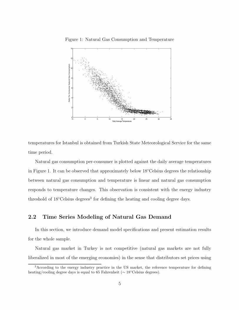
Figure 1: Natural Gas Consumption and Temperature

−5 0 5 10 15 20 25 30 350

2

4

6

8

10

12

14

Daily Average Temperatures

Dai

ly P

er C

onsu

mer

Nat

ural

Gas

Con

sum

ptio

n

temperatures for Istanbul is obtained from Turkish State Meteorological Service for the same

time period.

Natural gas consumption per-consumer is plotted against the daily average temperatures

in Figure 1. It can be observed that approximately below 18!Celsius degrees the relationship

between natural gas consumption and temperature is linear and natural gas consumption

responds to temperature changes. This observation is consistent with the energy industry

threshold of 18!Celsius degrees3 for defining the heating and cooling degree days.

2.2 Time Series Modeling of Natural Gas Demand

In this section, we introduce demand model specifications and present estimation results

for the whole sample.

Natural gas market in Turkey is not competitive (natural gas markets are not fully

liberalized in most of the emerging economies) in the sense that distributors set prices using

3According to the energy industry practice in the US market, the reference temperature for definingheating/cooling degree days is equal to 65 Fahrenheit (" 18"Celsius degrees).

5

a constant mark-up which is determined by a governmental agency, EMRA (Energy Market

Regulatory Authority). Since natural gas prices do not reflect changes in demand conditions,

demand estimation can be abstracted from possible supply side simultaneity issues.

We consider di!erent model specifications for estimation of daily natural gas demand.

In Table 1 model specifications are presented. The levels of natural gas consumption per-

consumer, (ct) is the dependent variable in “Panel A”, whereas in “Panel B”, the natural

logarithm of consumption per-consumer (ln(ct)) is used. The explanatory variables and the

notation used are as follows: daily heating degree days (HDDt); daily cooling degree days

(CDDt)4 time trend (t); natural gas prices (pt); and the holiday dummy (Ht), which is used

to capture possible e!ects of holidays on consumption. In Model 5b, the price is also in

logarithmic form to estimate the price elasticity of demand directly. We define the daily

average temperature as the average of the maximum and minimum temperatures observed

at a particular measurement station during a given day. Using this definition of daily average

temperature, which is denoted by Tt (measured in Celsius degrees), we define the heating

degree day (HDD) as HDDt = max(18#Tt, 0). For a given day, if the temperature is below

18!Celsius degrees then this is considered as a heating degree day (HDD > 0). We define

CDD similarly as CDDt = max(Tt # 18, 0).

Demand estimation results in Table 2 indicate that HDDs (and therefore temperature)

is the driving factor of the natural gas demand. Even only using the constant and HDD as

explanatory variables, which corresponds to Model 1a in Table 1, we obtain an adjusted R2

of 0.91. By including other explanatory variables such as the price and holiday dummy, the

adjusted R2 only improves marginally.

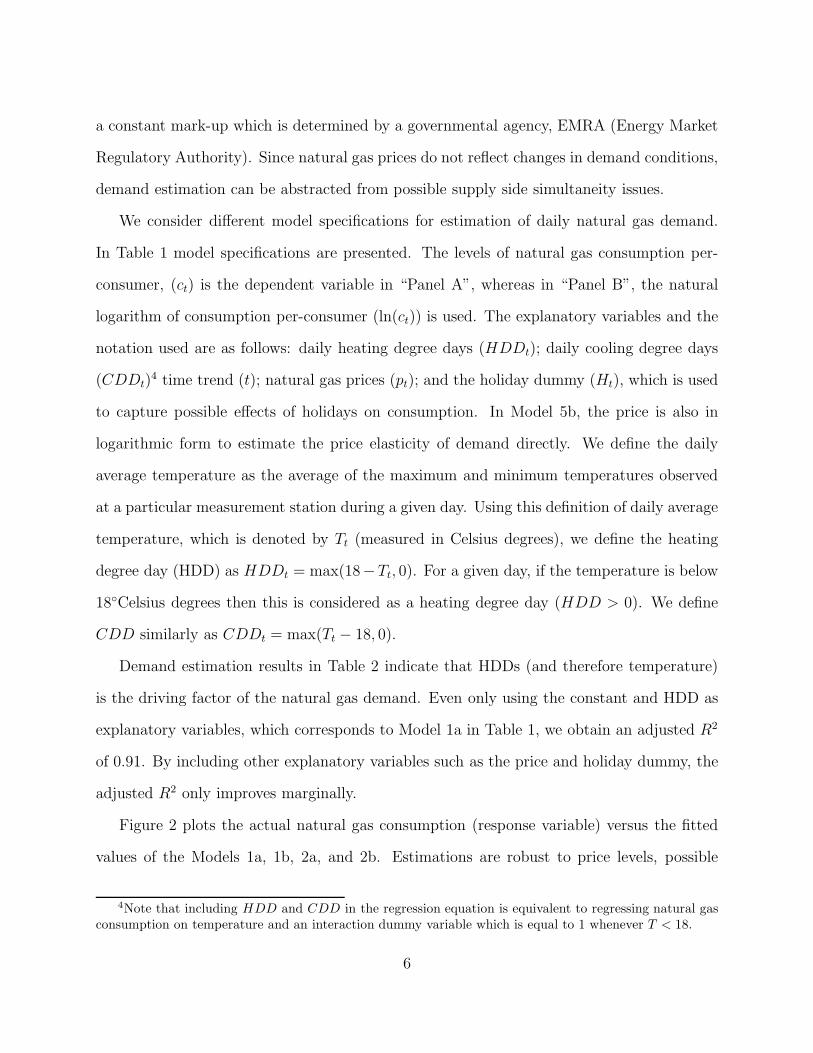
Figure 2 plots the actual natural gas consumption (response variable) versus the fitted

values of the Models 1a, 1b, 2a, and 2b. Estimations are robust to price levels, possible

4Note that including HDD and CDD in the regression equation is equivalent to regressing natural gasconsumption on temperature and an interaction dummy variable which is equal to 1 whenever T < 18.

6

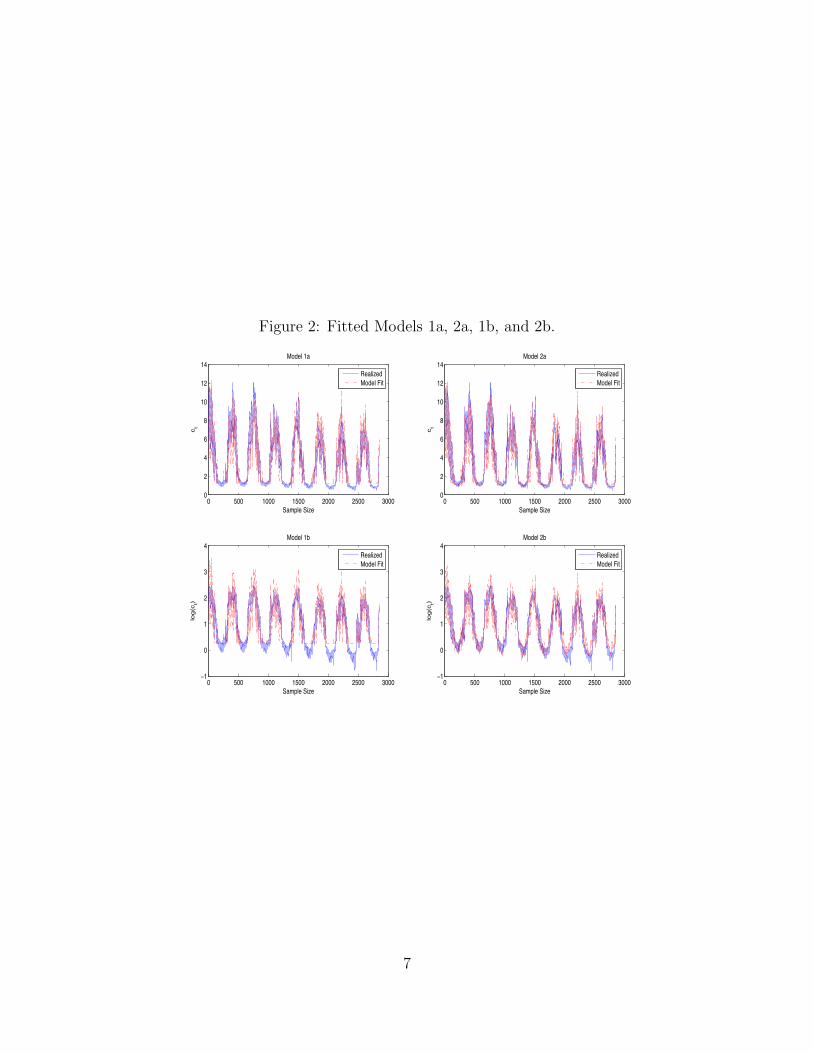
Figure 2: Fitted Models 1a, 2a, 1b, and 2b.

0 500 1000 1500 2000 2500 30000

2

4

6

8

10

12

14

Sample Size

c t

Model 1a

RealizedModel Fit

0 500 1000 1500 2000 2500 30000

2

4

6

8

10

12

14

Sample Size

c t

Model 2a

RealizedModel Fit

0 500 1000 1500 2000 2500 3000−1

0

1

2

3

4

Sample Size

log(

c t)

Model 1b

RealizedModel Fit

0 500 1000 1500 2000 2500 3000−1

0

1

2

3

4

Sample Size

log(

c t)

Model 2b

RealizedModel Fit

7

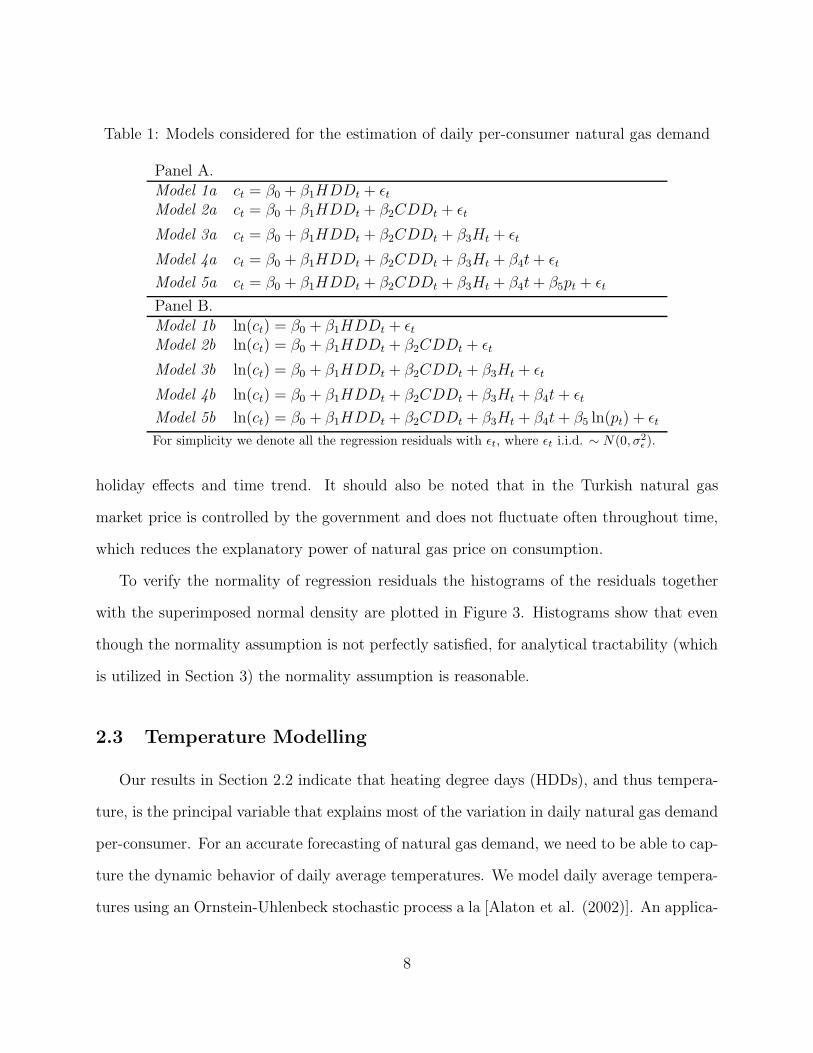
Table 1: Models considered for the estimation of daily per-consumer natural gas demand

Panel A.Model 1a ct = !0 + !1HDDt + "tModel 2a ct = !0 + !1HDDt + !2CDDt + "t

Model 3a ct = !0 + !1HDDt + !2CDDt + !3Ht + "t

Model 4a ct = !0 + !1HDDt + !2CDDt + !3Ht + !4t+ "tModel 5a ct = !0 + !1HDDt + !2CDDt + !3Ht + !4t+ !5pt + "tPanel B.Model 1b ln(ct) = !0 + !1HDDt + "tModel 2b ln(ct) = !0 + !1HDDt + !2CDDt + "t

Model 3b ln(ct) = !0 + !1HDDt + !2CDDt + !3Ht + "t

Model 4b ln(ct) = !0 + !1HDDt + !2CDDt + !3Ht + !4t+ "tModel 5b ln(ct) = !0 + !1HDDt + !2CDDt + !3Ht + !4t+ !5 ln(pt) + "tFor simplicity we denote all the regression residuals with !t, where !t i.i.d. " N(0,"2

! ).

holiday e!ects and time trend. It should also be noted that in the Turkish natural gas

market price is controlled by the government and does not fluctuate often throughout time,

which reduces the explanatory power of natural gas price on consumption.

To verify the normality of regression residuals the histograms of the residuals together

with the superimposed normal density are plotted in Figure 3. Histograms show that even

though the normality assumption is not perfectly satisfied, for analytical tractability (which

is utilized in Section 3) the normality assumption is reasonable.

2.3 Temperature Modelling

Our results in Section 2.2 indicate that heating degree days (HDDs), and thus tempera-

ture, is the principal variable that explains most of the variation in daily natural gas demand

per-consumer. For an accurate forecasting of natural gas demand, we need to be able to cap-

ture the dynamic behavior of daily average temperatures. We model daily average tempera-

tures using an Ornstein-Uhlenbeck stochastic process a la [Alaton et al. (2002)]. An applica-

8

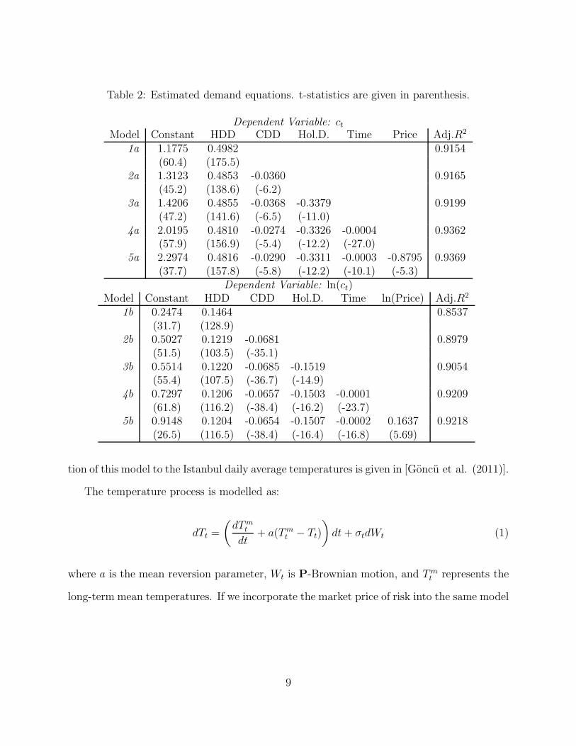
Table 2: Estimated demand equations. t-statistics are given in parenthesis.

Dependent Variable: ctModel Constant HDD CDD Hol.D. Time Price Adj.R2

1a 1.1775 0.4982 0.9154(60.4) (175.5)

2a 1.3123 0.4853 -0.0360 0.9165(45.2) (138.6) (-6.2)

3a 1.4206 0.4855 -0.0368 -0.3379 0.9199(47.2) (141.6) (-6.5) (-11.0)

4a 2.0195 0.4810 -0.0274 -0.3326 -0.0004 0.9362(57.9) (156.9) (-5.4) (-12.2) (-27.0)

5a 2.2974 0.4816 -0.0290 -0.3311 -0.0003 -0.8795 0.9369(37.7) (157.8) (-5.8) (-12.2) (-10.1) (-5.3)

Dependent Variable: ln(ct)Model Constant HDD CDD Hol.D. Time ln(Price) Adj.R2

1b 0.2474 0.1464 0.8537(31.7) (128.9)

2b 0.5027 0.1219 -0.0681 0.8979(51.5) (103.5) (-35.1)

3b 0.5514 0.1220 -0.0685 -0.1519 0.9054(55.4) (107.5) (-36.7) (-14.9)

4b 0.7297 0.1206 -0.0657 -0.1503 -0.0001 0.9209(61.8) (116.2) (-38.4) (-16.2) (-23.7)

5b 0.9148 0.1204 -0.0654 -0.1507 -0.0002 0.1637 0.9218(26.5) (116.5) (-38.4) (-16.4) (-16.8) (5.69)

tion of this model to the Istanbul daily average temperatures is given in [Goncu et al. (2011)].

The temperature process is modelled as:

dTt =

!

dTmt

dt+ a(Tm

t # Tt)

"

dt+ #tdWt (1)

where a is the mean reversion parameter, Wt is P-Brownian motion, and Tmt represents the

long-term mean temperatures. If we incorporate the market price of risk into the same model

9

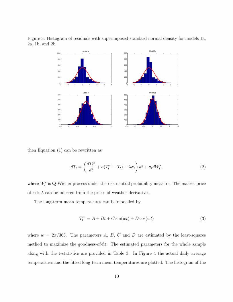
Figure 3: Histogram of residuals with superimposed standard normal density for models 1a,2a, 1b, and 2b.

−3 −2 −1 0 1 2 3 40

200

400

600

800

1000Model 1a

−3 −2 −1 0 1 2 3 40

200

400

600

800

1000Model 2a

−1.5 −1 −0.5 0 0.5 1 1.50

100

200

300

400

500

600Model 1b

−1.5 −1 −0.5 0 0.5 1 1.50

100

200

300

400

500

600Model 2b

then Equation (1) can be rewritten as

dTt =

!

dTmt

dt+ a(Tm

t # Tt)# $#t

"

dt+ #tdW"

t , (2)

where W "

t is Q-Wiener process under the risk neutral probability measure. The market price

of risk $ can be inferred from the prices of weather derivatives.

The long-term mean temperatures can be modelled by

Tmt = A+Bt+ C sin(wt) +D cos(wt) (3)

where w = 2%/365. The parameters A, B, C and D are estimated by the least-squares

method to maximize the goodness-of-fit. The estimated parameters for the whole sample

along with the t-statistics are provided in Table 3. In Figure 4 the actual daily average

temperatures and the fitted long-term mean temperatures are plotted. The histogram of the

10

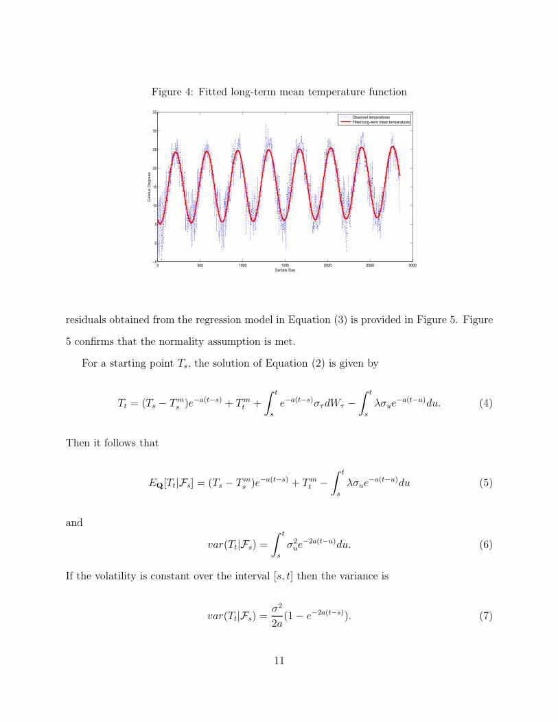
Figure 4: Fitted long-term mean temperature function

0 500 1000 1500 2000 2500 3000−5

0

5

10

15

20

25

30

35

Sample Size

Cel

sius

Deg

rees

Observed temperaturesFitted long−term mean temperatures

residuals obtained from the regression model in Equation (3) is provided in Figure 5. Figure

5 confirms that the normality assumption is met.

For a starting point Ts, the solution of Equation (2) is given by

Tt = (Ts # Tms )e#a(t#s) + Tm

t +

# t

s

e#a(t#s)#!dW! #

# t

s

$#ue#a(t#u)du. (4)

Then it follows that

EQ[Tt|Fs] = (Ts # Tms )e#a(t#s) + Tm

t #

# t

s

$#ue#a(t#u)du (5)

and

var(Tt|Fs) =

# t

s

#2ue

#2a(t#u)du. (6)

If the volatility is constant over the interval [s, t] then the variance is

var(Tt|Fs) =#2

2a(1# e#2a(t#s)). (7)

11

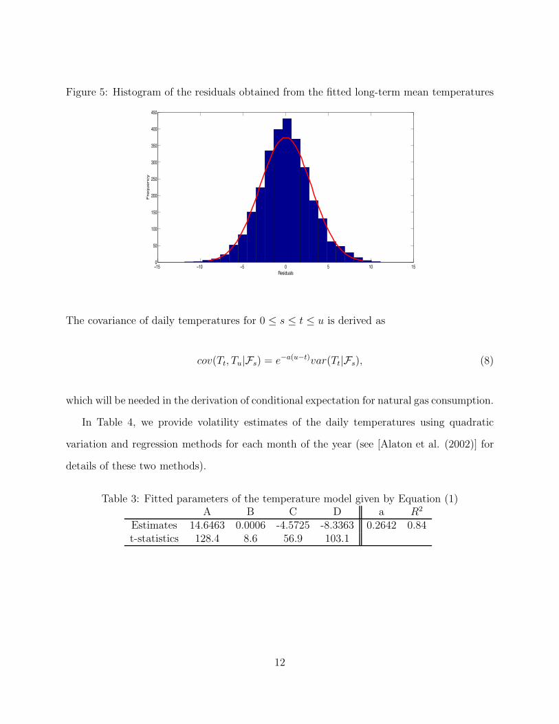
Figure 5: Histogram of the residuals obtained from the fitted long-term mean temperatures

−15 −10 −5 0 5 10 150

50

100

150

200

250

300

350

400

450

Residuals

Fre

qu

en

cy

The covariance of daily temperatures for 0 $ s $ t $ u is derived as

cov(Tt, Tu|Fs) = e#a(u#t)var(Tt|Fs), (8)

which will be needed in the derivation of conditional expectation for natural gas consumption.

In Table 4, we provide volatility estimates of the daily temperatures using quadratic

variation and regression methods for each month of the year (see [Alaton et al. (2002)] for

details of these two methods).

Table 3: Fitted parameters of the temperature model given by Equation (1)A B C D a R2

Estimates 14.6463 0.0006 -4.5725 -8.3363 0.2642 0.84t-statistics 128.4 8.6 56.9 103.1

12

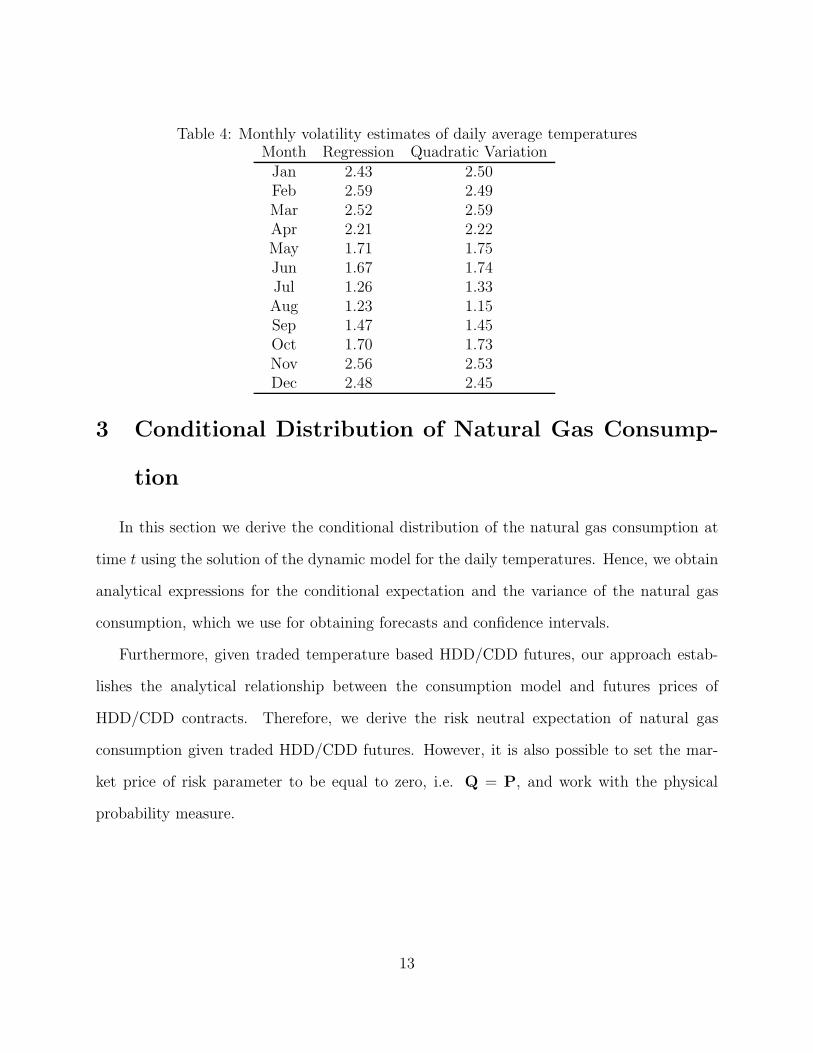
Table 4: Monthly volatility estimates of daily average temperaturesMonth Regression Quadratic VariationJan 2.43 2.50Feb 2.59 2.49Mar 2.52 2.59Apr 2.21 2.22May 1.71 1.75Jun 1.67 1.74Jul 1.26 1.33Aug 1.23 1.15Sep 1.47 1.45Oct 1.70 1.73Nov 2.56 2.53Dec 2.48 2.45

3 Conditional Distribution of Natural Gas Consump-

tion

In this section we derive the conditional distribution of the natural gas consumption at

time t using the solution of the dynamic model for the daily temperatures. Hence, we obtain

analytical expressions for the conditional expectation and the variance of the natural gas

consumption, which we use for obtaining forecasts and confidence intervals.

Furthermore, given traded temperature based HDD/CDD futures, our approach estab-

lishes the analytical relationship between the consumption model and futures prices of

HDD/CDD contracts. Therefore, we derive the risk neutral expectation of natural gas

consumption given traded HDD/CDD futures. However, it is also possible to set the mar-

ket price of risk parameter to be equal to zero, i.e. Q = P, and work with the physical

probability measure.

13

3.1 Derivation of the Conditional Distribution of Natural Gas

Consumption

We will consider two model specifications, Model 4a and 4b, respectively. However, the

same approach can be applied to other model specifications considered in previous section.

Model 4a is given by:

ct = !0 + !1HDDt + !2CDDt + !3Ht + !4t+ "t, "t " iid N(0, #2" ). (9)

Tt is normally distributed with the given mean and variance in Equations (5) and (6),

respectively. For any day t, we have either heating or cooling degree day, i.e. HDD % 0

or CDD > 0. We set & := {t|HDD % 0}, then the conditional expectation of natural gas

consumption for day t at day s (s < t) follows as

EQ[ct|t & &,Fs] = !0 + !1(18# EQ[Tt|Fs]) + !3Ht + !4t (10)

and

EQ[ct|t /& &,Fs] = !0 + !2(EQ[Tt|Fs]# 18) + !3Ht + !4t. (11)

Variance of the conditional natural gas consumption is calculated as follows

var(ct|t & &,Fs) = !21var(Tt|Fs) + #2

" (12)

and

var(ct|t /& &,Fs) = !22var(Tt|Fs) + #2

" . (13)

Denote the mean and variance of ct|t & & as µct,1 and #2ct,1, respectively. Then ct|t & & "

N(µct,1, #2ct,1), whereas the mean and variance of ct|t /& & is denoted as µct,0 and #2

ct,0. Then

14

ct|t /& & " N(µct,0, #2ct,0).

For simplicity suppose we want to obtain a forecast of natural gas consumption during

a winter month, where HDDt is always positive. We should also note that forecasting the

natural gas during winter months is particularly important due to the peaking natural gas

consumption.

Suppose given the information at time s we want to forecast C(t1, tM |Fs) := ct1+ct2+...+

ctM , where cti denotes the per-consumer natural gas consumption for day i and t1, ..., tM & &.

Then the conditional expectation and variance of C(t1, tM |Fs) is given by

EQ[C(t1, tM)|Fs] =M$

i=1

[!0 + !1(18#EQ[Tti |Fs]) + !3Ht + !4t], (14)

where EQ[Tti |Fs] is given in Equation (5). The variance is given by (s $ t1)

var(C(t1, tM |Fs)) =M$

i=1

%

!21var(Tti |Fs) + #2

"

&

+ 2$

i<j

cov(Tti , Ttj |Fs), (15)

where the variance and covariance of temperatures are given in Equations (7) and (8), re-

spectively. By substitution we obtain

var(C(t1, tM |Fs)) =M$

i=1

'

!21#

2

2a(1# e#2a(ti#s)) + #2

"

(

(16)

+ 2$

i<j

e#a(tj#ti)#2

2a(1# e#2a(tj#ti)).

Next, we consider Model 4b where the dependent variable is the logarithm of the natural

gas consumption. Similarly, we derive the conditional expectation under this alternative

model specification. Model 4b is given by:

log(ct) = !0 + !1HDDt + !2CDDt + !3Ht + !4t+ "t, "t iid " N(0, #2" ). (17)

15

Similarly, due to the normality of temperatures the natural gas consumption is log-

normally distributed. Then ct|t & & " Log-Normal(µct,1, #2ct,1), whereas ct|t /& & "

Log-Normal(µct,0, #2ct,0). Then the conditional expectation of natural gas consumption for

s < t is given by

EQ[ct|t & &,Fs] = exp(µct,1 + #2ct,1/2) (18)

and

EQ[ct|t /& &,Fs] = exp(µct,0 + #2ct,0/2). (19)

The variance is given by

var(ct| & &,Fs) = e(2µct,1+#2ct,1

)(e#2ct,1 # 1) (20)

and

var(ct| /& &,Fs) = e(2µct,0+#2ct,0

)(e#2ct,0 # 1). (21)

3.2 Risk-neutral expectation of natural gas consumption in the

existence of temperature-based futures

In this section, we derive a relationship between the conditional expectation of natural

gas consumption and temperature based futures contracts. For example, various types of

temperature futures such as, heating degree days (HDDs), cooling degree days (CDDs) and

cumulative average temperatures (CAT), are traded in the Chicago Mercantile Exchange

(CME). Next, we establish a connection between futures prices of HDD/CDD contracts and

natural gas consumption.

We consider Model 4a. From Equation (10) for t1, ..., tM & & we obtain the risk neutral

16

expectation of natural gas consumption as:

EQ[C(t1, tM)|Fs] =M$

i=1

[!0 + !1EQ[HDDti|Fs] + !3Ht + !4t] (22)

=M$

i=1

[!0 + !3Ht + !4t] + !1FHDD(t1, tM),

where FHDD(t1, tM) is the market price of HDD futures contract for the measurement period

[t1, tM ].

Similarly, from Equation (11) for t1, ..., tM /& & we obtain

EQ[C(t1, tM)|Fs] =M$

i=1

[!0 + !2EQ[CDDti|Fs] + !3Ht + !4t] (23)

=M$

i=1

[!0 + !3Ht + !4t] + !2FCDD(t1, tM),

where FCDD(t1, tM) is the market price of CDD futures contract for the measurement period

[t1, tM ].

4 Backtesting

In this section, we evaluate the forecast performance of the considered models via back-

testing method at monthly and 10-day forecast horizons. Realized per-consumer natural gas

consumption values are compared with the model forecasts from Monte Carlo simulation

and the conditional expectation derived in the previous section. Below, we describe our

methodology which relies on an iterative process for obtaining model forecasts at di!erent

time horizons. Without loss of generality, we only describe the backtesting procedure at

monthly forecast horizon.

1. We estimate the demand and temperature models using the first 365 days of our sample

17

i.e. we use data from January 1, 2004 to December 31, 2004. This part of the sample

is used for model estimation only.

2a. (Monte Carlo Simulation) For the the first consequent month (for the period January

1, 2005 to January 31, 2005), we simulate temperature and natural gas consumption

paths for each day using the simulated temperatures as an input in the demand model.

2b. (Conditional Expectation - Analytical Solution) Using the results in Section 3 we calcu-

late the conditional expectation of the natural gas consumption for the next consequent

month (for the period January 1, 2005 to January 31, 2005).

3. At the next step, we expand estimation window by including the consequent month

and repeat previous steps, i.e. we re-estimate both the demand and temperature

models, which allows us to use all the realized information to obtain the forecast of

the consequent month.

4. We repeat this iterative procedure until all the forecasts are obtained within the back-

testing sample.

In Figure 6 and 7 we plot the realized values for monthly and 10-day periods of the

natural gas consumption versus the forecasts obtained using Model 4a. The model performs

well in forecasting the level and the seasonality of natural gas consumption.

We evaluate forecast performance of the model by comparing realized and forecasted

consumption values for two di!erent forecast horizons, namely 10-day and monthly horizons.

We define Ci and Ci as

Ci =$

j

ci,tj and Ci =$

j

ci,tj , (24)

18

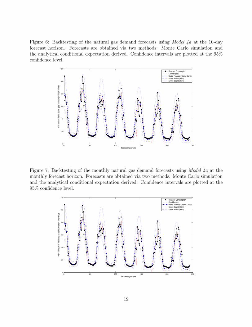
Figure 6: Backtesting of the natural gas demand forecasts using Model 4a at the 10-dayforecast horizon. Forecasts are obtained via two methods: Monte Carlo simulation andthe analytical conditional expectation derived. Confidence intervals are plotted at the 95%confidence level.

0 50 100 150 200 2500

20

40

60

80

100

120

Backtesting sample

Per−c

onsu

mer

nat

ural

gas

con

sum

ptio

n (m

onth

ly)

Realized ConsumptionCond.Expect.Model Forecast (Monte Carlo)Upper Bound (95%)Lower Bound (95%)

Figure 7: Backtesting of the monthly natural gas demand forecasts using Model 4a at themonthly forecast horizon. Forecasts are obtained via two methods: Monte Carlo simulationand the analytical conditional expectation derived. Confidence intervals are plotted at the95% confidence level.

0 50 100 150 200 2500

20

40

60

80

100

120

Backtesting sample

Per−c

onsu

mer

nat

ural

gas

con

sum

ptio

n (m

onth

ly)

Realized ConsumptionCond.Expect.Model Forecast (Monte Carlo)Upper Bound (95%)Lower Bound (95%)

19

where tj denotes the day of a given month i, cij and cij are the realized and forecasted

consumption on j th day of month i, respectively.

For a quantitative comparison of di!erent models, the relative mean square errors

(RMSE) are calculated by the following formula

1

N

N$

i=1

)

Ci # Ci

Ci

*2

, (25)

where i = 1, 2, ..., N denotes the number of months used in the backtesting sample, Ci

represents the model forecast for the ith month backtesting sample, whereas Ci represents

the actual monthly natural gas demand per-consumer.

The RMSE results for the considered models are compared in Table 5. Minimum RMSE

is achieved in Model 4a for Monte Carlo simulation and in Model 5b for analytical solution.

A more detailed comparison of Models 4a and 4b are provided in Table 6 at the monthly

forecast horizon.5 As expected, forecasts based on the conditional expectation of natural gas

consumption is particularly more accurate for winter or summer months, which reduces the

need for a Monte Carlo simulation. However, the accuracy of the analytical result decays

during transition months when it is more likely that temperature fluctuates around the

threshold value 18!C.

Since natural gas demand for space heating purposes peaks during winter months, fore-

casting accuracy for these periods is more critical. Monthly RMSE of forecasts based on

both Monte Carlo simulation and analytical solution suggest that -especially for consump-

tion levels (ct)- forecasting errors are lowest for winter months.

5For space considerations we only present RMSE results at the monthly forecast horizon.

20

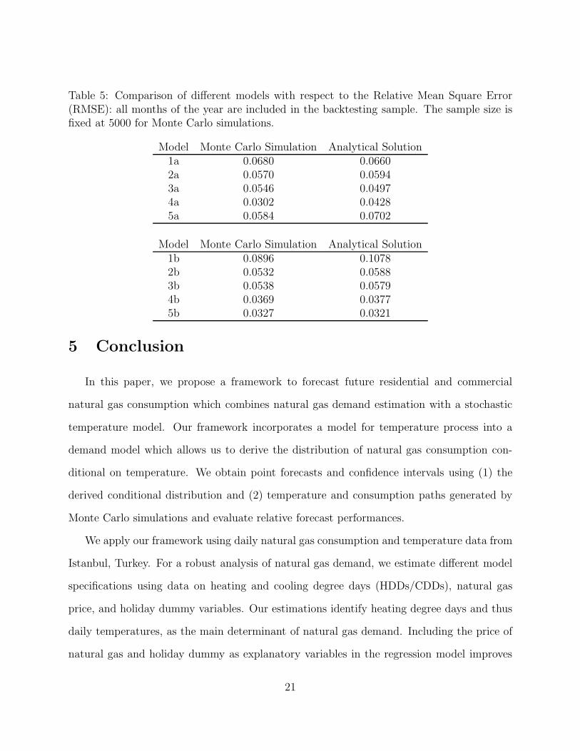
Table 5: Comparison of di!erent models with respect to the Relative Mean Square Error(RMSE): all months of the year are included in the backtesting sample. The sample size isfixed at 5000 for Monte Carlo simulations.

Model Monte Carlo Simulation Analytical Solution1a 0.0680 0.06602a 0.0570 0.05943a 0.0546 0.04974a 0.0302 0.04285a 0.0584 0.0702

Model Monte Carlo Simulation Analytical Solution1b 0.0896 0.10782b 0.0532 0.05883b 0.0538 0.05794b 0.0369 0.03775b 0.0327 0.0321

5 Conclusion

In this paper, we propose a framework to forecast future residential and commercial

natural gas consumption which combines natural gas demand estimation with a stochastic

temperature model. Our framework incorporates a model for temperature process into a

demand model which allows us to derive the distribution of natural gas consumption con-

ditional on temperature. We obtain point forecasts and confidence intervals using (1) the

derived conditional distribution and (2) temperature and consumption paths generated by

Monte Carlo simulations and evaluate relative forecast performances.

We apply our framework using daily natural gas consumption and temperature data from

Istanbul, Turkey. For a robust analysis of natural gas demand, we estimate di!erent model

specifications using data on heating and cooling degree days (HDDs/CDDs), natural gas

price, and holiday dummy variables. Our estimations identify heating degree days and thus

daily temperatures, as the main determinant of natural gas demand. Including the price of

natural gas and holiday dummy as explanatory variables in the regression model improves

21

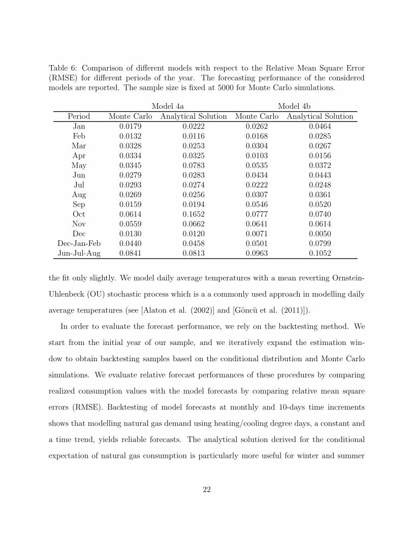
Table 6: Comparison of di!erent models with respect to the Relative Mean Square Error(RMSE) for di!erent periods of the year. The forecasting performance of the consideredmodels are reported. The sample size is fixed at 5000 for Monte Carlo simulations.

Model 4a Model 4bPeriod Monte Carlo Analytical Solution Monte Carlo Analytical SolutionJan 0.0179 0.0222 0.0262 0.0464Feb 0.0132 0.0116 0.0168 0.0285Mar 0.0328 0.0253 0.0304 0.0267Apr 0.0334 0.0325 0.0103 0.0156May 0.0345 0.0783 0.0535 0.0372Jun 0.0279 0.0283 0.0434 0.0443Jul 0.0293 0.0274 0.0222 0.0248Aug 0.0269 0.0256 0.0307 0.0361Sep 0.0159 0.0194 0.0546 0.0520Oct 0.0614 0.1652 0.0777 0.0740Nov 0.0559 0.0662 0.0641 0.0614Dec 0.0130 0.0120 0.0071 0.0050

Dec-Jan-Feb 0.0440 0.0458 0.0501 0.0799Jun-Jul-Aug 0.0841 0.0813 0.0963 0.1052

the fit only slightly. We model daily average temperatures with a mean reverting Ornstein-

Uhlenbeck (OU) stochastic process which is a a commonly used approach in modelling daily

average temperatures (see [Alaton et al. (2002)] and [Goncu et al. (2011)]).

In order to evaluate the forecast performance, we rely on the backtesting method. We

start from the initial year of our sample, and we iteratively expand the estimation win-

dow to obtain backtesting samples based on the conditional distribution and Monte Carlo

simulations. We evaluate relative forecast performances of these procedures by comparing

realized consumption values with the model forecasts by comparing relative mean square

errors (RMSE). Backtesting of model forecasts at monthly and 10-days time increments

shows that modelling natural gas demand using heating/cooling degree days, a constant and

a time trend, yields reliable forecasts. The analytical solution derived for the conditional

expectation of natural gas consumption is particularly more useful for winter and summer

22

months, which reduces the need for a Monte Carlo simulation. However, during transition

months we observe that the accuracy of the analytical result decays.

Furthermore, we establish a relationship between traded temperature-based weather

derivatives and expected natural gas consumption. Using our approach, if a weather deriva-

tives market exists for the considered location, then the implied natural gas demand per-

consumer with respect to the risk neutral probability measure can be derived. As a result,

this relationship allows for partial hedging of the demand risk of natural gas suppliers via

weather derivatives.

References

Alaton, P.,Djehiche, B., and Stillberger, D. 2002. On Modelling and Pricing Weather Deriva-

tives. Applied Mathematical Finance, 9, 1-20.

Aras, H. and Aras, N. 2004. Forecasting Residential Natural Gas Demand. Energy Sources,

26, 463-472.

Crompton, P., and Wu, Y. 2005. Energy consumption in China: past trends and future

directions. Energy Economics, 27, 195-208.

Erdogdu, E. 2010. Natural gas demand in Turkey Applied Energy 87 211-219.

Goncu, A., Karahan, M. O., and Kuzubas, T. U. 2011. Pricing of Temperature-based Weather

Options for Turkey. Iktisat Isletme ve Finans, 26, 33-50.

Gumrah, F., Katircioglu, D., Aykan, Y., Okumus, S., and Kilincer, N. 2001. Modeling of Gas

Demand Using Degree-Day Concept: Case Study for Ankara, Energy Sources, 23, 101-114.

Ediger, V., Akar, S., 2007. ARIMA forecasting of primary energy demand by fuel in Turkey.

Energy Policy, 35, 1701-1708.

23

Liu, L. M. and Lin, M. W. 1991. Forecasting residential consumption of natural gas using

monthly and quarterly time series. International Journal of Forecasting, 7, 3-16.

Potocnik, P., Thaler,M., Govekar, E., Grabec,I., Poredos,A., 2007. Forecasting risks of nat-

ural gas consumption in Slovenia. Energy Policy 35 4271-4282

Sanchez-Ubeda, E., and Berzosa, A. 2007. Modeling and forecasting industrial end-use nat-

ural gas consumption. Energy Economics, 29, 710-742

Sarak, H., and Satman, A. 2003. The degree-day method to estimate the residential heating

natural gas consumption in Turkey: a case study. Energy, 28, 929-939.

M.I.T. Energy Initiative 2011. The future of natural gas: an interdisciplinary MIT study,

24