Forecasting Complex Time Series - Inria

Forecasting Complex Time Series:Beanplot Time Series

Carlo Drago and Germana Scepi

Dipartimento di Matematica e Statistica

Università “Federico II” di Napoli

COMPSTAT 2010 19° International Conference on Computational Statistics Paris-France, August 22-27

http://www-roc.inria.fr/axis/COMPSTAT2010/welcome.html

The Aim

Forecasting Complex Time Series Paris, August 22 -27, 2010

Dealing with “complex” time series:

Scalar

Time Series

Bean Plot Time Series

Visualizing (CLADAG 2009,Gfkl 2010)

Synthesizing the global dynamics

ParametrizationBeanplot

Time Series

AttributeTime

Series

Forecasting

Beanplot

dynamics

Attribute

Time Series

Forecasting beanplot dynamics

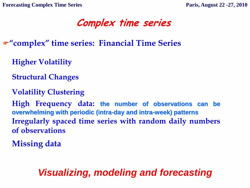
Complex time series

“complex” time series: Financial Time Series

Higher Volatility

Structural Changes

Volatility Clustering

High Frequency data: the number of observations can be

overwhelming with periodic (intra-day and intra-week) patterns

Irregularly spaced time series with random daily numbersof observations

Missing data

Visualizing, modeling and forecasting


Beanplot time series

A beanplot time series is an ordered sequence of beanplots overthe time. Each temporal interval can be considered as a domain ofvalues that is related to the chosen interval temporal (daily, week,and month).

The beanplot can be considered as a particular case of an interval-valued modal variable at the same time like boxplots andhistograms (see Arroyo and Mate 2006)

In a beanplot variable we are taking into account at the sametime the intervals of minimum and maximum and the density inform of a kernel nonparametric estimator (the density trace seeKampstra 2008).

Kernel

Bandwidth


Beanplot time series

From visualizing to clustering complex financial data... Karlsruhe, July 21 -23, 2010

Bean line

Minimum

Maximum

The beanplot time series show the complex structure of the underlyingphenomenon by representing jointly the data location (the bean line)the size (the interval between minimum and maximum) and theshape (the density trace) over the time

Bump

The bumps represent the values of maximum density showingimportant equilibrium values reached in a single temporal interval.Bumps can also show the intra-period patterns over the time and morein general the beanplot shape shows the intra-period dynamic

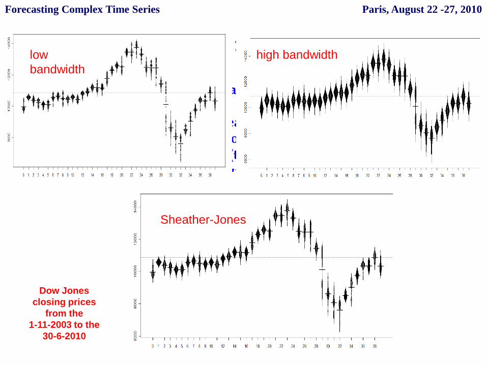
We can consider as fundamental the bandwidth.

With an higher bandwidth the beanplot gives a smoothed visualizationof the entire representation. So we need to choose carefully theparameter for the bandwidth (there are a lot of criteria, such asSheather-Jones method, see Kampstra 2008). The bandwidth becomesan index of volatility at time t.

Beanplot time serieslow

bandwidth

high bandwidth

Sheather-Jones

Dow Jones

closing prices

from the

1-11-2003 to the

30-6-2010


Attribute time series

For each time t we consider an internal model represented by eachBeanplot

For each time t we can consider n descriptors of the beanplots

Each descriptor is represented over the time as an attribute time series(see Matè and Arroyo ,2008)

By the attribute time series we take into account the dynamics of thephenomenon. In this sense we can consider the correlation over the timeof the beanplot features


Attribute time series (1)

At each time t from the kernel density estimate we consider theminimum, maximum, center and some coefficients from a polynomialmodel.

x


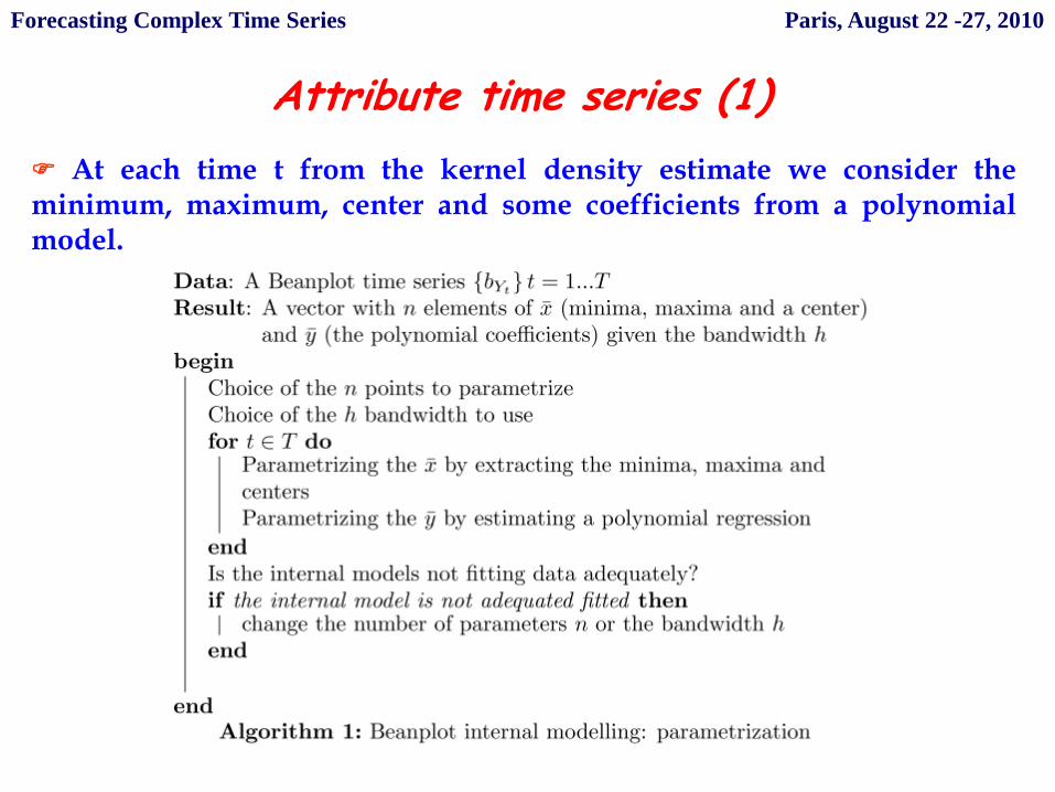
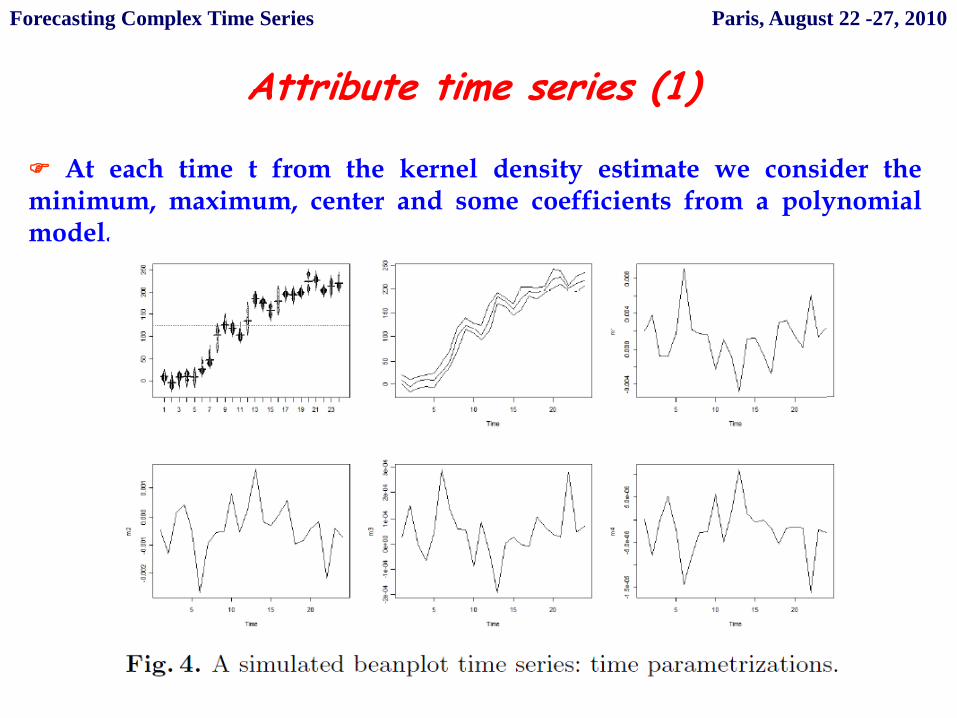
Attribute time series (2)

Alternative: at each time t from the kernel density estimate we canobtain n parameters as coordinates x y


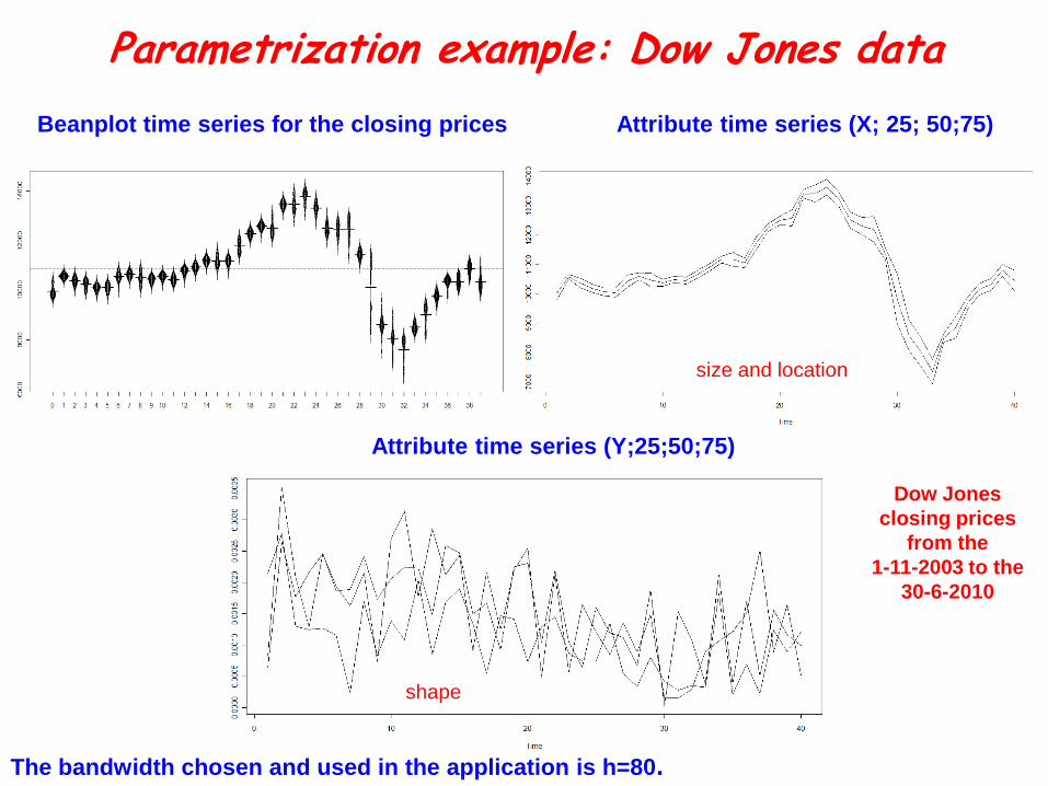
Parametrization example: Dow Jones data

Beanplot time series for the closing prices Attribute time series (X; 25; 50;75)

Attribute time series (Y;25;50;75)

The bandwidth chosen and used in the application is h=80.

Dow Jones

closing prices

from the

1-11-2003 to the

30-6-2010

size and location

shape

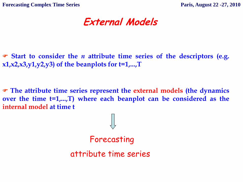
External Models

Start to consider the n attribute time series of the descriptors (e.g.x1,x2,x3,y1,y2,y3) of the beanplots for t=1,...,T

The attribute time series represent the external models (the dynamicsover the time t=1,...,T) where each beanplot can be considered as theinternal model at time t

Forecasting

attribute time series


Forecasting methods

Univariate Methods (ARIMA, Smoothing Splines, Neural Networks,Hybrid Methods)

Multivariate Methods (VAR, VECM)

Forecasts combination

Univariate methods when there is not an explicit relationship between the attributes with/or without autocorrelation

Multivariate methods if a correlation explicitly exists


Forecasting Procedure

Start to consider the n attribute time series of the descriptors of thebeanplots for t=1,...,T. They represent the beanplot dynamics over thetime

Checking for the stationarity and the autocorrelation. Detecting thefeatures of the dynamics (trends, cycles, seasonality). Analyzing therelationships between the attributes

Forecasting them using a specific method

Considering as Beanplot description the forecasts obtained from theForecasting Method.

Diagnostics


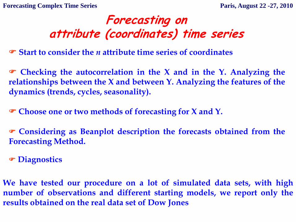
Forecasting on attribute (coordinates) time series

Start to consider the n attribute time series of coordinates

Checking the autocorrelation in the X and in the Y. Analyzing therelationships between the X and between Y. Analyzing the features of thedynamics (trends, cycles, seasonality).

Choose one or two methods of forecasting for X and Y.

Considering as Beanplot description the forecasts obtained from theForecasting Method.

Diagnostics

We have tested our procedure on a lot of simulated data sets, with highnumber of observations and different starting models, we report only theresults obtained on the real data set of Dow Jones


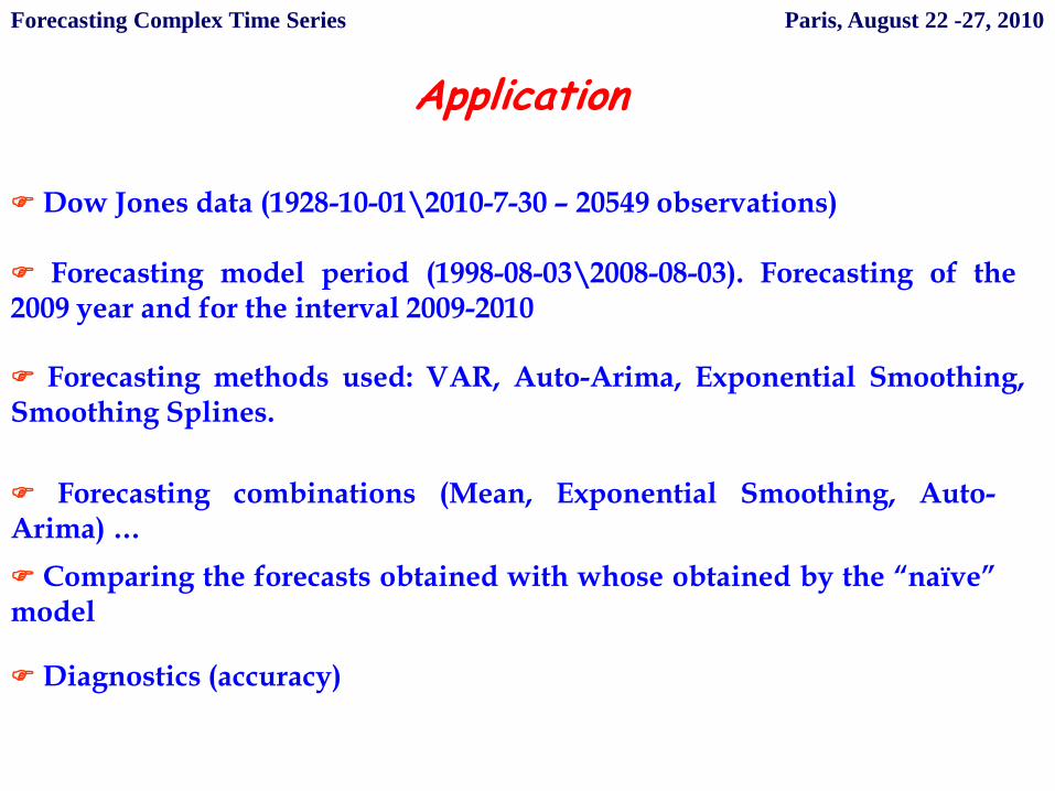
Application

Dow Jones data (1928-10-01\2010-7-30 – 20549 observations)

Forecasting model period (1998-08-03\2008-08-03). Forecasting of the2009 year and for the interval 2009-2010

Comparing the forecasts obtained with whose obtained by the “naïve”model

Forecasting methods used: VAR, Auto-Arima, Exponential Smoothing,Smoothing Splines.

Forecasting combinations (Mean, Exponential Smoothing, Auto-Arima) …

Diagnostics (accuracy)


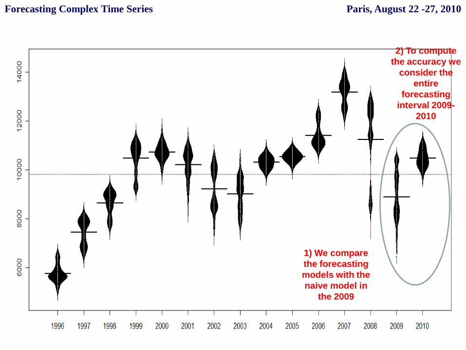
1) We compare

the forecasting

models with the

naive model in

the 2009

2) To compute

the accuracy we

consider the

entire

forecasting

interval 2009-

2010


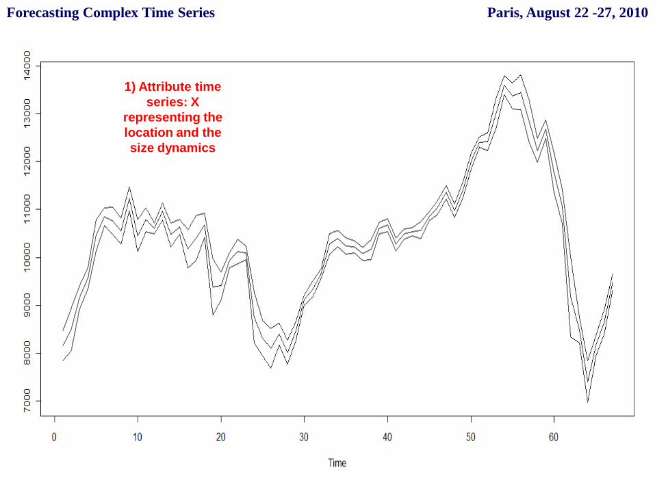
1) Attribute time

series: X

representing the

location and the

size dynamics


1) Attribute time

series: Y

representing the

shape dynamics


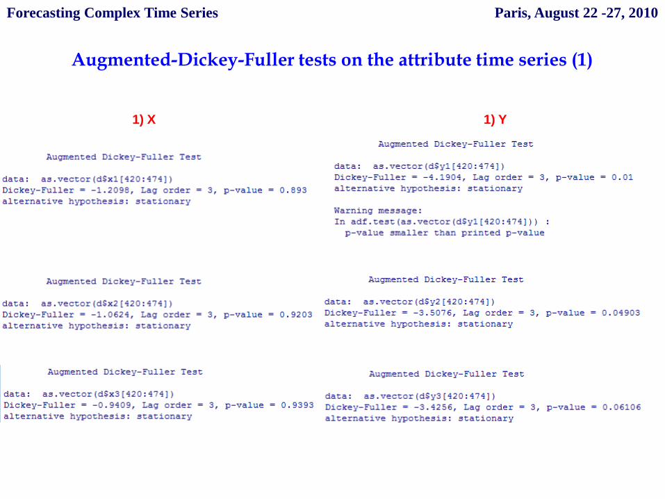
Augmented-Dickey-Fuller tests on the attribute time series (1)

1) X 1) Y


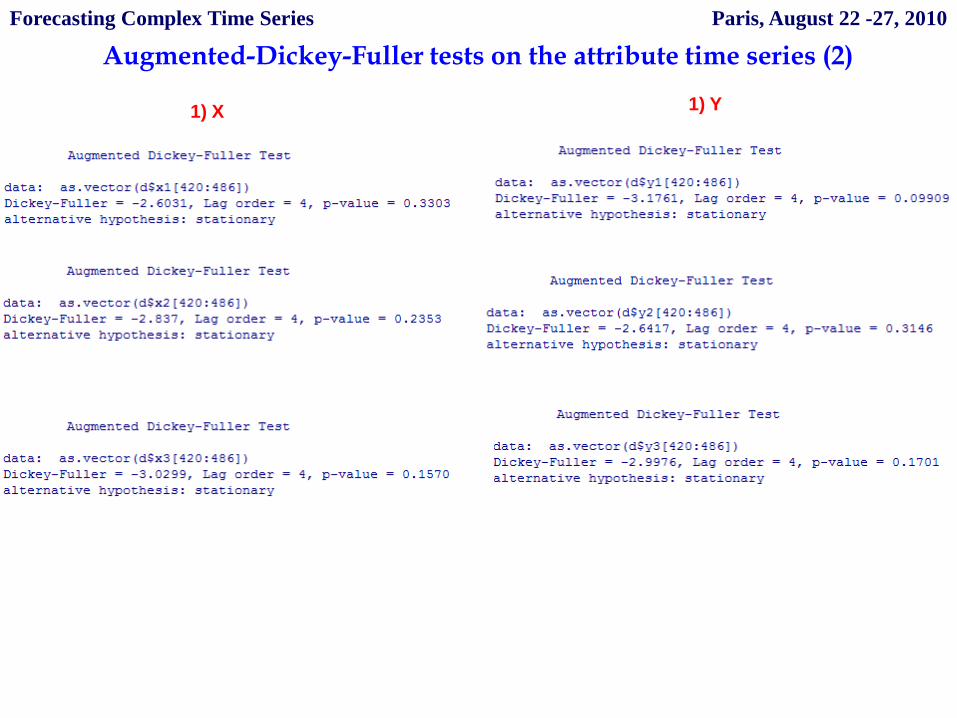
Augmented-Dickey-Fuller tests on the attribute time series (2)

1) Y 1) X


X- Attribute Time Series Phillips-Ouliaris Cointegration test

Year 1998-2008

All observations


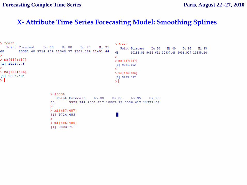
X- Attribute Time Series Forecasting Model: Smoothing Splines


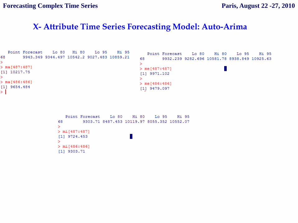
X- Attribute Time Series Forecasting Model: Auto-Arima


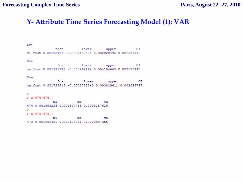
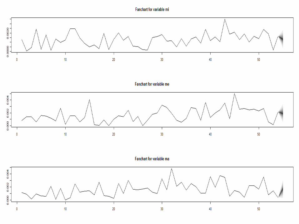
Y- Attribute Time Series Forecasting Model (1): VAR


Y- Attribute Time Series Forecasting Model (2): Smoothing Splines


Accuracy of the X - Forecasting Model: Smoothing Splines

Me

Mi

Ma


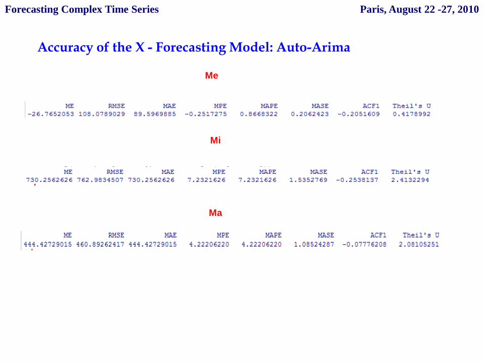
Accuracy of the X - Forecasting Model: Auto-Arima

Me

Mi

Ma


Accuracy of the Y - Forecasting Model: VAR


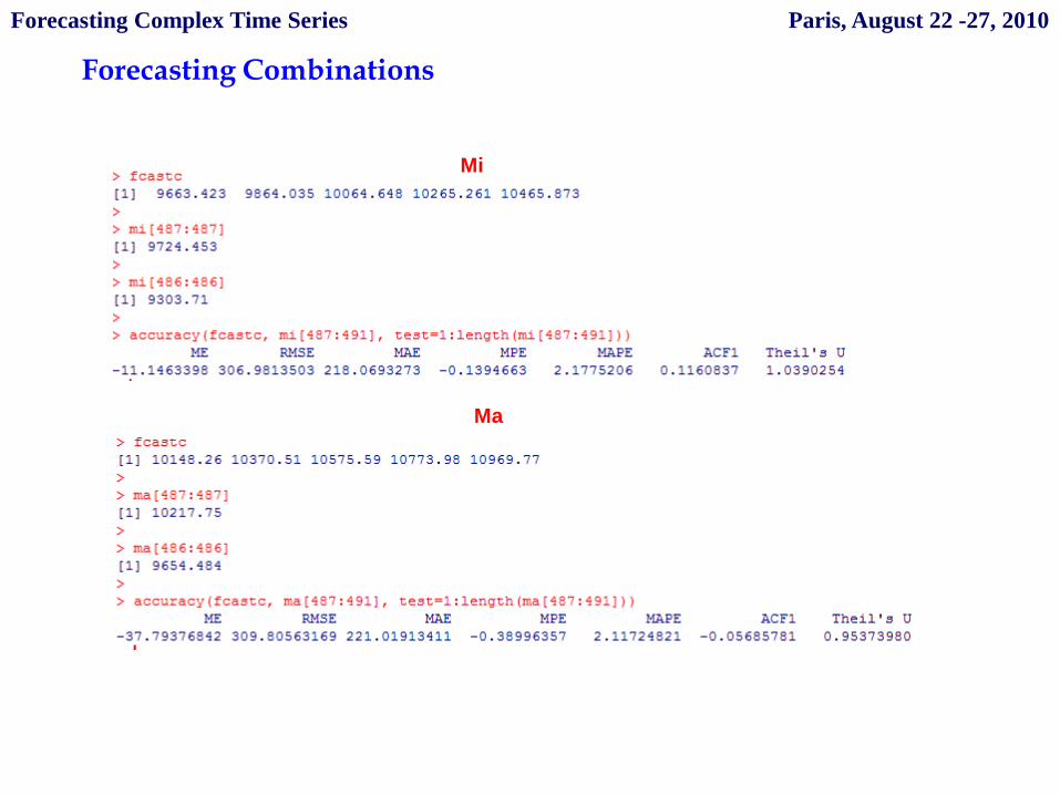
Forecasting Combinations

Mi

Ma


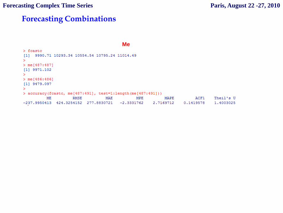
Forecasting Combinations

Me


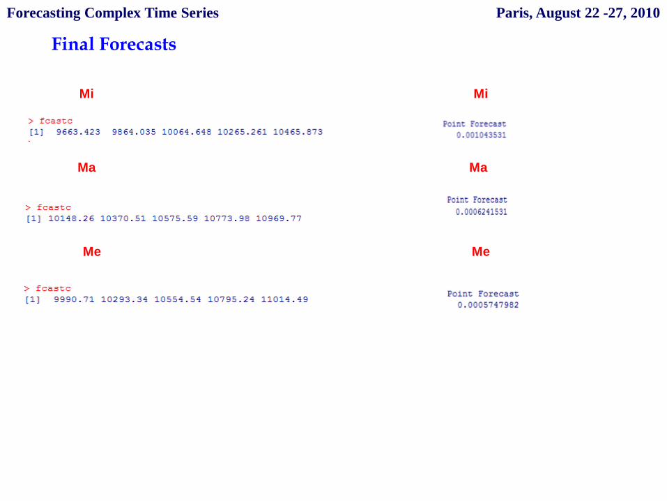
Final Forecasts

Mi

Ma

Me

Ma

Me

Mi


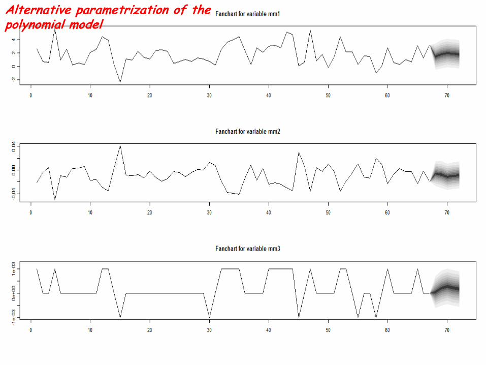
Alternative parametrization of the polynomial model

Some developments

From visualizing to clustering complex financial data... Karlsruhe, July 21 -23, 2010

Beanplot clustering of different beanplot time series and consideringthem in a Forecasting Model (see Drago Scepi 2010 presented atGfkl\Cladag in Karlsruhe).

Forecasts Combinations using different forecasting methods

Multivariate case: Cointegration (Long run and short run)

Beanplot TSFAan internal parametrization, where it is crucial to fit adequately (or usefully) the data.

Some References

•Arroyo J. , Gonzales Rivera G., and Matè C. (2009) “Forecasting with Interval and HistogramData: Some Financial Applications”. Working Paper•Arroyo J., Matè C. (2009) ” Forecasting Histogram Time Series with K-Nearest NeighboursMethods” International Journal of Forecasting, 25, pp.192-207•Billard, L., Diday, E. (2006) Symbolic data analysis: conceptual statistics and data mining.Chichester: Wiley & Sons.•Dacorogna B. et al. (2001) An Introduction of High Frequency Finance. Academic Press.•Drago C., Scepi G. (2010) “Forecasting by Beanplot Time Series” Electronic Proceedings ofCompstat/, Springer Verlag, p.959-967, ISBN 978-3-7908-2603-6•Drago C., Scepi G. (2010) “Visualizing and exploring high frequency financial data:beanplot time series” accettato su : /New Perspectives in Statistical Modeling and DataAnalysis, Springer Series: Studies in Classification, Data Analysis, andKnowledge Organization, Ingrassia, Salvatore; Rocci, Roberto; Vichi, Maurizio (Eds), ISBN:978-3-642-11362, atteso per novembre 2010•Engle, R.F, Russel J.R. (2004) “Analysis of High Frequency Financial Data” Working Paper.•Kampstra, P. (2008) Beanplot: “A Boxplot Alternative for Visual Comparison of Distributions”Journal of Statistical Software Vol. 28, Code Snippet 1, Nov. 2008•Meijer E., Gilbert P.D. (2005) “Time Series Factor Analysis with an Application to MeasuringMoney” SOM Research Report, University of Groningen.•Sheather, S. J. and Jones, M. C. (1991). A reliable data-based bandwidth selection method forkernel density estimation. JRSS-B 53, 683-690.•Yan, B., Zivot G. (2003).Analysis of High-Frequency Financial Data with S-PLUS.WorkingPaper.

Forecasting Complex Time Series - Inria

Documents

Transcript of Forecasting Complex Time Series - Inria