Introduction to (Demand) Forecasting

Topics

• Introduction to (demand) forecasting• Overview of forecasting methods• A generic approach to quantitative forecasting• Time series-based forecasting• Building causal models through multiple linear

regression• Confidence Intervals and their application in forecasting

Forecasting• The process of predicting the values of a certain quantity,

Q, over a certain time horizon, T, based on past trends and/or a number of relevant factors.

• Some forecasted quantities in manufacturing– demand– equipment and employee availability– technological forecasts– economic forecasts (e.g., inflation rates, exchange rates, housing

starts, etc.)

• The time horizon depends on– the nature of the forecasted quantity– the intended use of the forecast

Forecasting future demand

• Demand forecasting is based on:– extrapolating to the future past trends observed in the company

sales;– understanding the impact of various factors on the company future

sales:• market data• strategic plans of the company• technology trends• social/economic/political factors• environmental factors• etc

• Remark: The longer the forecasting horizon, the more crucial the impact of the factors listed above.

Demand Patterns

• The observed demand is the cumulative result of:– systematic variation, due to a number of identified factors, and– a random component, incorporating all the remaining unaccounted

effects.

• Patterns of systematic variation– seasonal: cyclical patterns related to the calendar (e.g., holidays,

weather)– cyclical: patterns related to changes of the market size, due to, e.g.,

economics and politics– business: patterns related to changes in the company market share,

due to e.g., marketing activity and competition– product life cycle: patterns reflecting changes to the product life

The problem of demand forecasting

– Identify and characterize the systematic variation, as a set of trends.

– Characterize the variability in the demand.

Forecasting Methods

• Qualitative (Subjective): Incorporate factors like the forecaster’s intuition, emotions, personal experience, and value system.

• These methods include:– Jury of executive opinion– Sales force composites– Delphi method– Consumer market surveys

Forecasting Methods (cont.)

• Quantitative (Objective): Employ one or more mathematical models that rely on historical data and/or causal/indicator variables to forecast demand.

• Major methods include:– time series methods: F(t+1) = f (D(t), D(t-1), …)– causal models: F(t+1) = f(X1(t), X2(t), …)

Selecting a Forecasting Method• It should be based on the following considerations:

– Forecasting horizon (validity of extrapolating past data)– Availability and quality of data– Lead Times (time pressures)– Cost of forecasting (understanding the value of

forecasting accuracy)– Forecasting flexibility (amenability of the model to

revision; quite often, a trade-off between filtering out noise and the ability of the model to respond to abrupt and/or drastic changes)

Implementing Quantitative ForecastingDetermine Method•Time Series•Causal Model

Collect data:<Ind.Vars; Obs. Dem.>

Fit an analytical model to the data:

F(t+1) = f(X1, X2,…)

Use the model forforecasting future demand

Monitor error:e(t+1) = D(t+1)-F(t+1)

ModelValid?

Update ModelParameters

Yes No

- Determine functional form- Estimate parameters- Validate

Time Series-based Forecasting

Basic Model:

HistoricalData

,...2,1),(ˆ =+ ττtDtiiD ,...,1),( =Forecasts

Time Series Model

Remark: The exact model to be used depends on the expected /observed trends in the data.Cases typically considered:• Constant mean series• Series with linear trend• Series with seasonalities (and possibly a linear trend)

A constant mean series

0.00

2.00

4.00

6.00

8.00

10.00

12.00

14.00

1 2 3 4 5 6 7 8 9 10 11 12 13 14 15 16 17 18 19 20

Series1

The above data points have been sampled from a normal distribution with a mean value equal to 10.0 and a variance equal to 4.0.

Forecasting constant mean series:The Moving Average model

The presumed model for the observed data:

)()( teDtD +=where

D is the constant mean of the series and

)(te is normally distributed with zero mean and some unknownvariance

2σThen, under a Moving Average of Order N model, denoted as MA(N),the estimate of returned at period t, is equal to:D

∑−

=

−=1

0

)(1

)(ˆN

i

itDN

tD

The forecasting error

• The forecasting error

• Also

∑−

=

+−−=+−=+1

0

)1()(1

)1()(ˆ)1(N

i

tDitDN

tDtDtε

∑−

=

=−=+−−=+1

0

0)(1

)]1([)]([1

)]1([N

i

DDNN

tDEitDEN

tE ε

∑−

=

+=+=++−=+1

0

22222

)1

1(1

)]1([)]([1

)]1([N

i NN

NtDVaritDVar

NtVar σσσε

Forecasting error (cont.)

∀ ε(t+1) is normally distributed with the mean and variance computed in the previous slide.

• follows a normal distribution with zero mean and variance σ2/N.

DtD −)(ˆ

Selecting an appropriate order N

• Smaller values of N provide more flexibility.• Larger values of N provide more accuracy (c.f., the formula for the variance of the forecasting error).• Hence, the more stable (stationary) the process, the larger the N.• In practice, N is selected through trial and error, such that it minimizes one of the following criteria:

i)

ii)

iii)

∑+=−

=t

Ni

tNt

tMAD1

|)(|1

)( ε

∑+=−

=t

Ni

tNt

tMSD1

2))((1

)( ε

∑+=−

=t

Ni tD

t

NttMAPE

1 )(

)(1)(

ε

Demonstrating the impact of N on the model performance

0.00

5.00

10.00

15.00

20.00

25.00

1 4 7 10

13

16

19

22

25

28

31

34

37

40

Series1

Series2

Series3

• blue series: the original data series, distributed according to N(10,4) for the first 20 points, and N(20,4) for the last 20 points.• magenta series: the predictions of the MA(5) forecasting model.• yellow series: the predictions of the MA(10) forecasting model. • Remark: the MA(5) model adjusts faster to the experienced jump of the data mean value, but the mean estimates that it provides under stationary operation are less accurate than those provided by the MA(10) model.

Forecasting constant mean series:The Simple Exponential Smoothing model

• The presumed demand model:

)()( teDtD +=where is an unknown constant and is normally distributed with zero mean and an unknown variance .

D )(te2σ

• The forecast , at the end of period t:)(ˆ tD

)]1(ˆ)([)1(ˆ)1(ˆ)1()()(ˆ −−+−=−−+= tDtDatDtDataDtD

where α∈(0,1) is known as the “smoothing constant”.

• Remark: The updating equation constitutes a correction of the previous estimate in the direction suggested by the forecasting error, )1(ˆ)( −− tDtD

Expanding the Model Recursion

)1(ˆ)1()()(ˆ −−+= tDataDtD

€

=aD(t)+a(1−a)D(t−1)+(1−a)2 D (t−2)=.................................................................................................

∑−

=

−+−−=1

0

)0(ˆ)1()()1(t

i

ti DaitDaa

Implications

1. The model considers all the past observations and the initializing value in the determination of the estimate .

2. The weight of the various data points decreases exponentially with their age.

3. As α→1, the model places more emphasis on the most recent observations.

4. As t→∞,

)(ˆ tD)0(D

DtDE →)](ˆ[ and 2

2

2)](ˆ)1([ σ

atDtDVar

−→−+

The impact of α and of on the model performance

0.00

5.00

10.00

15.00

20.00

25.00

1 4 7 10

13

16

19

22

25

28

31

34

37

40

Series1

Series2

Series3

Series4

)0(D

• dark blue series: the original data series, distributed according to N(10,4) for the first 20 points, and N(20,4) for the last 20 points. • magenta series: the predictions of the ES(0.2) model initialized at the value of 10.0.• yellow series: the predictions of the ES(0.2) model initialized as 0.0.• light blue series: the predictions of the ES(0.8) model initialized at 10.0. • Remark: the ES(0.8) model adjusts faster to the jump of the series mean value, but the estimates that it provides under stationary operation are less accurate than those provided by the ES(0.2) model. Also, notice that the effect of the initial value is only transient.

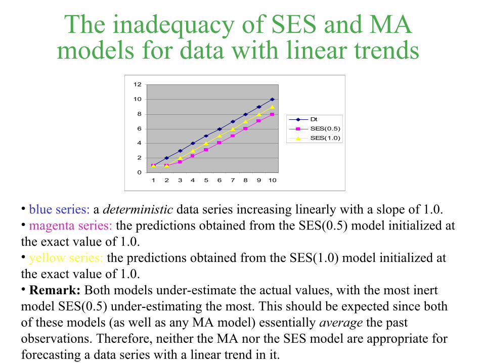
The inadequacy of SES and MA models for data with linear trends

0

2

4

6

8

10

12

1 2 3 4 5 6 7 8 9 10

Dt

SES(0.5)

SES(1.0)

• blue series: a deterministic data series increasing linearly with a slope of 1.0.• magenta series: the predictions obtained from the SES(0.5) model initialized at the exact value of 1.0.• yellow series: the predictions obtained from the SES(1.0) model initialized at the exact value of 1.0. • Remark: Both models under-estimate the actual values, with the most inert model SES(0.5) under-estimating the most. This should be expected since both of these models (as well as any MA model) essentially average the past observations. Therefore, neither the MA nor the SES model are appropriate for forecasting a data series with a linear trend in it.

Forecasting series with linear trend:The Double Exponential Smoothing Model

The presumed data model:

)()( tetTItD +⋅+=where

I is the model intercept, i.e., the unknown mean value for t=0,

)(te is normally distributed with zero mean and some unknownvariance

2σ

T is the model trend, i.e., the mean increase per unit of time, and

The Double Exponential Smoothing Model (cont.)

The parameters a and β take values in the interval (0,1) and are the model smoothing constants, while the values and are the initializing values.

The model forecasts at period t for periods t+τ, τ=1,2,…, are given by:

ττ ⋅+=+ )(ˆ)(ˆ)(ˆ tTtItD

with the quantities and obtained through the following recursions:

)(ˆ tI )(ˆ tT

)]1(ˆ)1(ˆ)[1()()(ˆ −+−−+⋅= tTtIatDatI

)1(ˆ)1()]1(ˆ)(ˆ[)(ˆ −⋅−+−−= tTtItItT ββ

)0(I )0(T

The Double Exponential Smoothing Model (cont.)

• The smoothing constants are chosen by trial and error, using the MAD, MSD and/or MAPE indices.• For t→∞, and • The variance of the forecasting error, , can be estimated as a function of the noise variance σ2 through techniques similar to those used in the case of the Simple Exp. Smoothing model, but in practice, it is frequently approximated by

where

for some appropriately selected smoothing constant γ∈(0,1) or by

ItI →)(ˆ TtT →)(ˆ2εσ

)(25.1ˆ 2 tMAD=εσ

)1()1()()( −−+= tMADttMAD γεγ

)(ˆ 2 tMSD=εσ

DES Example

0

2

4

6

8

10

12

1 2 3 4 5 6 7 8 9 10

Dt

DES(T0=1)

DES(T0=0)

• blue series: a deterministic data series increasing linearly with a slope of 1.0.• magenta series: the predictions obtained from the DES(0.5;0.2) model initialized at the exact value of 1.0.• yellow series: the predictions obtained from the DES(0.5;0.2) model initialized at the value of 0.0. • Remark: In the absence of variability in the original data, the first model is completely accurate (the blue and the magenta series overlap completely), while the second model overcomes the deficiency of the wrong initial estimate and eventually converges to the correct values.

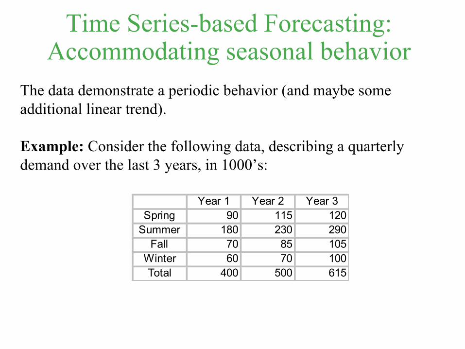
Time Series-based Forecasting:Accommodating seasonal behavior

The data demonstrate a periodic behavior (and maybe some additional linear trend).

Example: Consider the following data, describing a quarterly demand over the last 3 years, in 1000’s:

Year 1 Year 2 Year 3Spring 90 115 120

Summer 180 230 290Fall 70 85 105

Winter 60 70 100Total 400 500 615

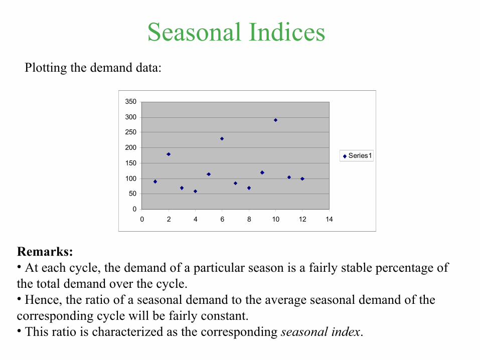
Seasonal Indices

0

50

100

150

200

250

300

350

0 2 4 6 8 10 12 14

Series1

Plotting the demand data:

Remarks: • At each cycle, the demand of a particular season is a fairly stable percentage of the total demand over the cycle.• Hence, the ratio of a seasonal demand to the average seasonal demand of the corresponding cycle will be fairly constant.• This ratio is characterized as the corresponding seasonal index.

A forecasting methodologyForecasts for the seasonal demand for subsequent years can be obtained by:ii. estimating the seasonal indices corresponding to the various seasons in the

cycle;iii. estimating the average seasonal demand for the considered cycle (using, for

instance, a forecasting model for a series with constant mean or linear trend, depending on the situation);

iv. adjusting the average seasonal demand by multiplying it with the corresponding seasonal index.

Example (cont.):

Year 1 Year 2 Year 3 SI(1) SI(2) SI(3) SISpring 90 115 120 0.9 0.92 0.78 0.87

Summer 180 230 290 1.8 1.84 1.88 1.84Fall 70 85 105 0.7 0.68 0.68 0.69

Winter 60 70 100 0.6 0.56 0.65 0.6Total 400 500 615 4 4 4 4

Average 100 125 153.75

Winter’s Method for Seasonal Forecasting

The presumed model for the observed data:

)()()( 1mod)1( tectTItD Nt +⋅⋅+= +−

where

• N denotes the number of seasons in a cycle;

• ci, i=1,2,…N, is the seasonal index for the i-th season in the cycle;

• I is the intercept for the de-seasonalized series obtained by dividing the original demand series with the corresponding seasonal indices;

• T is the trend of the de-seasonalized series;

• e(t) is normally distributed with zero mean and some unknown variance 2σ

Winter’s Method for Seasonal Forecasting (cont.)

The model forecasts at period t for periods t+τ, τ=1,2,…, are given by:

)(ˆ])(ˆ)(ˆ[)(ˆ1mod)1( tctTtItD Nt +−+⋅⋅+=+ τττ

where the quantities , and are obtained from the following recursions, performed in the indicated sequence:

)(ˆ tI )(ˆ tT ,,...,1),(ˆ Nitci =

)]1(ˆ)1(ˆ)[1()1(ˆ

)(:)(ˆ

1mod)1(

−+−−+−

=+−

tTtIatc

tDatI

Nt

)1(ˆ)1()]1(ˆ)(ˆ[:)(ˆ −⋅−+−−⋅= tTtItItT ββ

)1(ˆ)1()(ˆ)(

:)(ˆ 1mod)1(1mod)1( −⋅−+= +−+− tctI

tDtc NtNt γγ

1mod)1(),1(ˆ:)(ˆ +−≠∀−= Ntitctc ii

The parameters α, β, γ take values in the interval (0,1) and are the model smoothing constants, while and are the initializing values.

€

I (0), T (0) ,,...,1),0(ˆ Nici =

Causal Models:Multiple Linear Regression

• The basic model:

eXbXbbD kk +++⋅+= ...110

where• Xi, i=1,…,k, are the model independent variables (otherwise known as the explanatory variables);• bi, i=0,…,k, are unknown model parameters;• e is the a random variable following a normal distribution with zero mean and some unknown variance σ2.• D follows a normal distribution where ),( 2σDN

kk XbXbbD ⋅++⋅+= ...110

• We need to estimate <b0,b1,…,bk> and σ2 from a set of n observations

},...,1,,...,,;{ 21 njXXXD kjjjj =><

Estimating the parameters bi• The observed data satisfy the following equation:

+

=

nkknn

k

k

n e

e

e

b

b

b

XX

XX

XX

D

D

D

......

...1

............

...1

...1

...2

1

1

0

1

212

111

2

1

or in a more concise form

ebXd +⋅=• The vector

bXde ⋅−=denotes the difference between the actual observations and the corresponding mean values, and therefore, is selected such that it minimizes the Euclidean norm of the resulting vector .

bbXde ˆˆ ⋅−=

• The minimizing value for is equal to dXXXb TT 1)(ˆ −=• The necessary and sufficient condition for the existence of is that the columns of matrix X are linearly independent.

1)( −XX T

b

Characterizing the model variance• An unbiased estimate of σ2 is given by

1−−=

kn

SSEMSE

where

(Mean Squared Error)

)ˆ()ˆ(ˆˆ bXdbXdeeSSE TT ⋅−⋅−=⋅= (Sum of Squared Errors)

• The quantity SSE/σ2 follows a Chi-square distribution with n-k-1 degrees of freedom.

• Given a point x0T=(1,x10,…,xk0), an unbiased estimator of is given by)( 0xD

010100ˆ...ˆˆ)(ˆ

kk xbxbbxD ⋅++⋅+=• This estimator is normally distributed with mean and variance )( 0xD 0

10

2 )( xXXx TT −σ

• The random variable can function also as an estimator for any single observation D(x0). The resulting error will have zero mean and variance

)(ˆ0xD

)()(ˆ00 xDxD −

])(1[ 01

02 xXXx TT −+σ

Assessing the goodness of fit• A rigorous characterization of the quality of the resulting approximation can be obtained through Analysis of Variance, that can be traced in any introductory book on statistics.

•A more empirical test considers the coefficient of multiple determination

YYS

SSRR =2

where

∑=

−=−=n

jj

TT dDdndXbSSR1

22 )ˆ()(ˆ

∑=

=n

jjD

nd

1

1

and

SSRSSESYY +=• Remark: A natural way to interpret R2 is as the fraction of the variability in the observed data interpreted by the model over the total variability in this data.

Multiple Linear Regression and Time Series-based forecasting

• The model needs to be linear with respect to the parameters bi but not the explanatory variables Xi. Hence, the factor multiplying the parameter bi can be any function fi of the underlying explanatory variables.

• When the only explanatory variable is just the time variable t, the resulting multiple linear regression model essentially supports time-series analysis.

• The above approach for time-series analysis enables the study of more complex dependencies on time than those addressed by the moving average and exponential smoothing models.

• The integration of a new observation in multiple linear regression models is much more cumbersome than the updating performed by the moving average and exponential smoothing models (although there is an incremental linear regression model that alleviates this problem).

Confidence Intervals

• Confidence intervals are used in:ii. monitoring the performance of the applied forecasting model; iii. adjusting an obtained forecast in order to achieve a certain

performance level

• Given a random variable X and p∈(0,1), a p⋅100% confidence interval (CI) for it is an interval [a,b] such that

pbXaP =≤≤ )(

• The necessary confidence intervals are obtained by exploiting the statistics for the forecasting error, derived in the previous slides.

Variance estimation and the t distribution• The variance of the forecasting error is a function of the unknown variance, σ2, of the model disturbance, e.• E.g., in the case of multiple linear regression, the variance of the forecasting error is equal to .)()(ˆ

00 xDxD − ])(1[ 01

02 xXXx TT −+σ

• Hence, one cannot take advantage directly of the normality of the forecasting error in order to build the sought confidence intervals.• This problem can be circumvented by exploiting the fact that the quantity SSE/σ2 follows a Chi-square distribution with n-k-1 degrees of freedom.Then, the quantity

])(1[

)()(ˆ

1

)(1)]()(ˆ[

01

0

00

2

01

000

xXXxMSE

xDxD

knSSE

xXXxxDxDT

TT

TT

−

−

+⋅

−=

−−

+−=

σ

σ

follows a t distribution with n-k-1 degrees of freedom.

• For large samples, T can also be approximated by a standardized normal distribution.

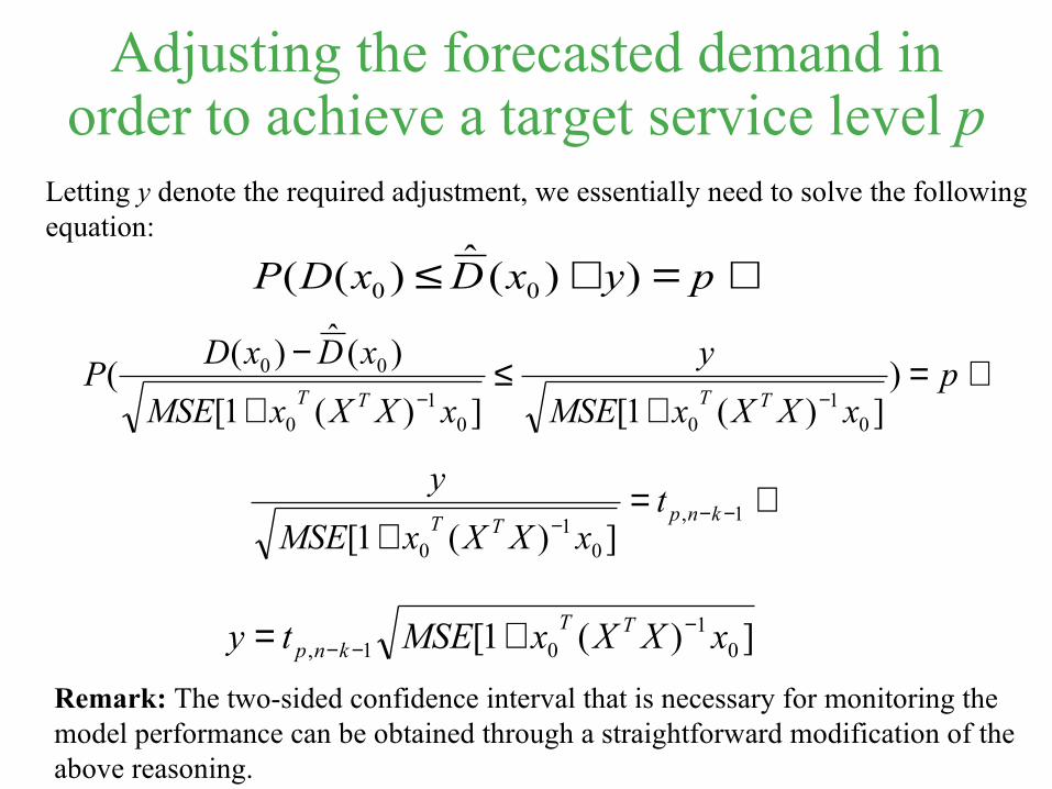
Adjusting the forecasted demand in order to achieve a target service level p

Letting y denote the required adjustment, we essentially need to solve the following equation:

⇔=+≤ pyxDxDP ))(ˆ)(( 00

⇔=+

≤+

−−−

pxXXxMSE

y

xXXxMSE

xDxDP

TTTT)

])(1[])(1[

)(ˆ)((

01

001

0

00

⇔=+

−−− 1,

01

0 ])(1[knp

TTt

xXXxMSE

y

])(1[ 01

01, xXXxMSEty TTknp

−−− +=

Remark: The two-sided confidence interval that is necessary for monitoring the model performance can be obtained through a straightforward modification of the above reasoning.