Fordham University Department of Economics Discussion ... · Fordham University Department of...

Fordham University Department of Economics Discussion Paper Series

How Investors Face Financial Risk Loss Aversion and Wealth Allocation

Erick Rengifo Fordham University Emanuela Trifan

J. W. Goethe University Frankfurt am Main

Discussion Paper No: 2008-01 January 2008

Department of Economics

Fordham University 441 E Fordham Rd, Dealy Hall

Bronx, NY 10458 (718) 817-4048

How Investors Face Financial Risk

Loss Aversion and Wealth Allocation ∗

Erick W. Rengifo† Emanuela Trifan‡

October 2007

∗The authors would like to thank Michel Baes, Marco Chiarandini, Horst Entorf, Ralf Hepp, Duncan

James, Bharath Rangarajan, Victor Ricciardi, Troy Tassier, the seminar participants at the Department of

Applied Economics and Econometrics of the Darmstadt University of Technology Meetings 2006 and 2007,

the NYC Computational Economics & Complexity Workshop 2006, the Eastern Financial Association

Meeting 2007, and the Society for the Advancement of Behavioral Economics Meeting 2007 for helpful

suggestions. The usual disclaimers apply.†Fordham University New York, Department of Economics. 441 East Fordham Road, Dealy Hall,

Office E513, Bronx, NY 10458, USA. Phone: +1 (718) 817 4061, fax: +1 (718) 817 3518, e-mail: rengi-

[email protected].‡J. W. Goethe University Frankfurt am Main, Department of Economics, Chair of Econometrics.

Mertonstr. 17 (PF 247), D-60054 Frankfurt am Main, Germany. Phone: +49 (0)69 798 28305, fax: +49

(0)69 798 28303, e-mail: [email protected].

How Investors Face Financial Risk

Loss Aversion and Wealth Allocation

October 2007

Abstract

We study how the wealth-allocation decisions and the loss aversion of non-

professional investors change subject to behavioral factors. The optimal wealth

assignment between risky and risk-free assets results within a VaR portfolio model,

where risk is individually assessed according to an extended prospect-theory frame-

work. We show how the past performance and the portfolio evaluation frequency

impact investor behavior. Myopic loss aversion holds at different evaluation fre-

quencies. One year is the optimal frequency at which, under practical constraints,

risky holdings are maximized. Previous research using standard VaR-significance

levels may underestimate the loss aversion of individual investors.

Keywords : prospect theory, myopic loss aversion, Value-at-Risk, portfolio evaluation, cap-

ital allocation

JEL Classification: G10, G11, D81, E27

1 Introduction

The main concern of investors in financial markets is how to optimally allocate money

among different (types of) assets. Portfolio theory teaches us that the optimal alloca-

tion results from the maximization of expected portfolio returns subject to given levels

of market risk. In spite of the appealing intuition and mathematical tractability, such an

optimization is not an easy task, especially for laymen. The reason is that it involves the

selection from a huge variety and quantity of financial instruments existent in practice,

and it often requires advanced mathematical skills. The natural response of real finan-

cial environments to this difficulty has been the specialization of the investment activity

between professionals and non-professionals. Non-professional investors – in other words

people whose main occupation does not concern financial investments and/or who lack

the necessary knowledge, expertise, time or any combination of them for making more

sophisticated investment decisions – rely often on the help of professional portfolio man-

agers in devising an optimal mix of risky assets. In other words, they often delegate the

security and asset allocation to professional managers.1

In particular, one can think of the decision process of non-professional investors as

unfolding in two main steps: First, they determine the total sum of money to be invested in

financial markets (in technical terms the budget constraint). Second, in order to optimally

split this money among different financial instruments, they ask for professional advice.

In so doing, they commit the technical details of the optimization of their asset portfolio

to professional managers, who dispose of sufficient resources to this end. Moreover, non-

professional investors provide managers with information about the level of risk they are

ready to bear (the risk constraint). Acting on this information, managers finally derive

the optimal capital allocation for their particular clients. What is important for non-

professionals in this context is simply how their wealth can be (optimally) split between

1In essence, this practical tendency of work division between non-professionals and professionals con-forms with portfolio theory. According to the top-down strategy, portfolio optimization can be describedby means of a threefold decision procedure: A first step, referred to as the capital allocation decision, dealswith the choice between risky and risk-free assets. A second so-called asset allocation decision focuses onthe further selection of different classes of risky assets. The third security allocation decision is concernedwith the specific securities to be held within each particular risky asset class chosen before. In practice,the last two decisions are usually made by professional portfolio managers with no intervention of their(non-professional) clients. By contrast, as far as the first decision is concerned the participation of thesenon-professionals becomes necessary, since it allows managers to determine the capital allocation thatbest fits the individual risk-profiles of their clients.

3

risky and risk-free assets.

It is the decision process of the non-professional investors that our paper focuses

on. This process – although of indisputable practical importance – has been somewhat

neglected in the literature sofar. The extensive research on portfolio optimization deals

with more sophisticated details, such as of choosing among different categories of risky

assets, that we consider to usually be the responsibility of the portfolio managers.

In particular, we are interested in how non-professionals split their money between

risky and risk-free assets. Since this decision depends on the individual risk profile, we

also study the investors’ attitude towards financial losses. Note that our work does not con-

tribute to the understanding of professional investors’ decisions, but gives insight into how

non-professional investors “operate” on financial markets. In our setting, non-professional

investors start from questioning what is their acceptable monetary loss from risky invest-

ments. This information depends on individual risk profiles that affect the quantity of

money that they are going to invest in risky assets. Also, the frequency of evaluating

risky portfolio changes the risk profile and hence their overall performance.

Our paper extends the portfolio optimization setting in Campbell, Huisman, and

Koedijk (2001), where risk is quantified in form of Value-at-Risk, by explicitly accounting

for the formation of what we denote as the individual VaR (VaR*). Our VaR* relies on

subjective perceptions of the non-professional investors and is formulated in line with the

extended prospect theory in Barberis, Huang, and Santos (2001).

We first analyze how non-professional investors set their subjective VaR*, specifically

contingent upon their loss aversion, the past performance of the risky portfolio, the cur-

rent value of the risky investment, and the expected risk premium. We show how VaR*

flows into the portfolio optimization undertaken by the professional manager in form of

a risk constraint. We derive the optimal wealth percentages to be invested in the risky

portfolio and in risk-free assets and study how they vary in time and subject to different

portfolio evaluation frequencies. Furthermore, we introduce an extended measure, termed

as the global first-order risk aversion (gRA), that attempts to provide additional infor-

mation concerning the loss attitude of non-professional investors. We comment on how

the frequency of evaluating risky performance can directly and indirectly impact on the

investors’ attitude towards risky investments and on how this twofold influence can be

4

estimated.

Our theoretical results are supported and amended by findings relying on the S&P 500

index and the US three-month treasury bills between 1982-2006. The past performance

appears to drive the current perception of the risky portfolio. Investors allocate on average

between 0-35% of their wealth to risky assets, where the main source of this substantial

fluctuation is the portfolio evaluation frequency. The proportion of risky investments

decreases fast when portfolio performance is checked more often than once a year, which

complies with the notion of myopic loss aversion introduced in Benartzi and Thaler (1995).

Furthermore, we conduct an extended analysis of the perceived utility of the risky

portfolio and of the loss attitude in what we denote as the evaluation-frequency domain.

Specifically, we propose a twofold segmentation in dependence on the portfolio evaluation

frequency of both the prospective value and the global first-order risk aversion. Merely

evaluation frequencies higher than one year are of practical relevance. In this context,

both variables suggest the frequency of one year as being optimal for generating positive

attitudes towards risky investments.

Finally, variables aimed at providing an equivalence between the traditional VaR-

approach and the estimates in our VaR*-framework – such as equivalent significance

levels, loss aversion coefficients, and investments in risky assets – point out that the actual

reluctance towards financial losses of non-professional investors might be underestimated.

The remainder of the paper is organized as follows. Section 2 presents the main

theoretical considerations. We start with a brief review of the optimal portfolio selection

model with exogenous VaR* by Campbell, Huisman, and Koedijk (2001), then take on the

value function formulation in Barberis, Huang, and Santos (2001). The notion of VaR* is

subsequently introduced. Finally, concentrating on how individual investors perceive the

value of the risky portfolio, we derive the prospective value and introduce our extended

measure of loss aversion. Section 3 illustrates the implementation of our theoretical model.

We discuss the impact of the evaluation frequency and of the past performance on the

wealth percentages invested in the risky portfolio. Also, we extensively investigate the

evolution of the prospective value and of the extended loss-attitude measure subject to

various evaluation frequencies. Our model is further restated in terms of previous research

with VaR risk constraints. Section 4 summarizes the results and concludes. Graphs and

5

further findings are included in the Appendix.

2 Theoretical model

This section contains the main theoretical considerations of our work. We start by re-

viewing the portfolio selection model in Campbell, Huisman, and Koedijk (2001). This

model uses VaR as its measure of risk. Our own setting, subsequently formulated, incor-

porates the individual perception of risky projects as captured in the extended prospect

theory framework of Barberis, Huang, and Santos (2001). We detail the construction of

our measure of individual loss aversion VaR* and its implications for the wealth allocation

decisions of non-professional investors. We also add to the formal representation of the in-

vestors’ attitude towards financial losses by introducing the notion of global first-order risk

aversion (gRA). Moreover, we briefly address how the prospective value and this extended

loss-attitude measure may vary subject to different portfolio evaluation frequencies.

2.1 Optimal portfolio selection with “exogenous” VaR

The model in Campbell, Huisman, and Koedijk (2001) follows the common procedure of

portfolio optimization, where market risk is assessed by means of Value-at-Risk (abbr.

VaR). In particular, financial assets are chosen in order to maximize expected returns,

subject to a twofold restriction: the budget and risk constraints. Investors can borrow or

lend extra money at the fixed market interest rate – which is equivalent with an investment

in risk-free assets. The maximum expected loss from holding the risky portfolio should

not exceed what we call an exogenous VaR (abbr. VaRex). This VaRex stands for the risk

level that the non-professional client is disposed to bear. It is indicated to the portfolio

manager in form of a single, fixed number.2 In this model, managers do not account for

how VaRex forms in the client perception. They consider it as constraint, exogenous to

the optimization problem.3

The objective of the optimization problem in Campbell, Huisman, and Koedijk (2001)

2The VaRex further enters the portfolio optimization problem in form of a threshold level, being thusexogenous to it.

3Specifically, managers interpret the client indication (a single number) in terms of the theoreticalconcept of VaR, i.e. of two elements: a confidence level and an investment horizon.

6

is maximizing the next-period wealth Wt+1. This wealth results from what the compo-

nents of the risky portfolio and the risk-free assets are expected to return. The risky

portfolio consists of i = 1, . . . , n financial assets with single time-t prices pi,t and portfolio

weights wi,t, such thatn∑

i=1

wi,t = 1. Moreover, ai,t is the number of shares of the asset i

contained in the portfolio at time t.4 Formally, we can state the portfolio optimization

problem as follows:

Wt+1(wt) = (Wt + Bt)Et[Rt+1(wt)]−BtRf −→wt

max. (1)

s.t.Wt + Bt =

n∑i=1

ai,tpi,t = a′tpt (budget constraint)

Pt[Wt+1(wt) ≤ Wt − VaRex] ≤ 1− α (risk constraint),

(2)

where Rt+1(wt) stands for the portfolio gross returns at the next trade and Et[Rt+1(wt)]

for the corresponding expected returns. Henceforth, we refer to the gross returns of the

risky portfolio by “returns” or “portfolio returns” .

In the above Equations (1) and (2), Bt denotes the risk-free investment, i.e. the sum

of money that can be borrowed (Bt > 0) or lent (Bt < 0) at the fixed risk-free gross

return rate Rf . Note that the maximization in Equation (1) is carried over the weights of

the risky portfolio wt but not over Bt. The risk-free investment results as a by-product

of the optimization procedure.5 Finally, Pt denotes the conditional probability given the

information at time t, and 1− α the chosen confidence level.

After some manipulations, Campbell, Huisman, and Koedijk (2001) obtain the optimal

weights of the risky portfolio as:

woptt ≡ arg max

wt

Et[Rt+1(wt)]−Rf

WtRf −Wtqt(wt, α), (3)

where qt(wt, α) represents the quantile of the distribution of portfolio gross returns Rt+1(wt)

for the confidence level 1 − α (or significance α), i.e. Pt[Rt+1(wt) ≤ qt(wt, α)] ≤ 1 − α.

Thus, the optimal mix of risky assets depends merely on the distribution of the portfolio

4Clearly, ai,t = wi,t(Wt + Bt)/pi,t.5See the comments concerning the two-fund separation below.

7

gross returns and on the significance level α.

Equation (3) shows that, similarly to the traditional mean-variance framework, the

two-fund separation theorem applies: Neither the (non-professional) investors’ initial wealth

nor the desired risk level VaRex affects the maximization procedure. In other words, in-

vestors first determine the optimal risky portfolio (i.e. the optimal allocation among

different risky assets) and second, they decide upon the extra amount of money to be

borrowed or lent (i.e. invested in risk-free assets). The latter reflects by how much the

portfolio VaR, that is defined as:

VaRt = Wt

(qt(w

optt , α)− 1

), (4)

varies according to the investor degree of loss aversion measured by the selected (desired)

VaRex-level.6

The optimal investment in risk-free assets can be then written as:

Bt =VaRex + VaRt

Rf − qt(woptt , α)

, (5)

and hence the value of the risky investment at time t + 1 yields:

St+1 = (Wt + Bt)Rt+1. (6)

Since we consider that non-professionals are mainly concerned with how to split their

money between risky and risk-free assets, the optimal investments in risk-free and risky

assets in Equations (5) and (6) represent fundamental variables in our model. Note that

we do not further elaborate on the optimal weights of the risky assets in Equation (3),

as the details of wealth allocation among the different risky portfolio components are

assumed to be left in charge of portfolio managers.

6Note that VaRex is imposed by the client prior to the portfolio formation and enters the portfoliooptimization problem in form of a constraint. By contrast, the portfolio VaR is an output of this opti-mization and measures the actual maximum loss that can be incurred at time t at the confidence level1− α for the obtained optimal portfolio wopt

t .

8

2.2 The individual loss level VaR*

Coming from the main ideas of the setting in Campbell, Huisman, and Koedijk (2001),

our model goes a step further by asking how non-professional investors actually arrive at

their desired level of loss aversion. We elaborate on the construction of an individual loss

level, that we denote as VaR*, and on its implications for the wealth allocation between

risky and risk-free assets. As far as the optimization procedure presented in the above

Section 2.1 is concerned, we can think of VaR* formally replacing VaRex in the above

equations, but remaining an exogenous input (constraint). However, the value of this risk

constraint forms now, according to our approach, on the basis of individual behavioral

parameters and affects the final wealth allocation between risky and risk-free assets, as

apparent from Equation (5). This extension of the allocation problem7 motivates us to

denote VaR* as the endogenous individual loss level.

2.2.1 The value function

Investors’ desires and attitudes – hence their subjective level VaR* – depend on their

perception of the value of financial investments. The prospect theory (abbr. PT) in Kah-

neman and Tversky (1979) and Tversky and Kahneman (1992) suggests how individual

perceptions of financial performance can be formalized by means of the so-called value

function v.8 Accordingly, human minds take for actual carriers of value not the absolute

outcomes of a project, but their changes defined as departures from an individual reference

point. The deviations above (below) this reference are labeled as gains (losses). Thus, the

value function is kinked at the reference point and exhibits distinct profiles in the domains

of gains and losses, being steeper for losses (a property known as loss aversion). It also

shows diminishing sensitivity in both domains, i.e. it is concave for gains but convex for

losses.

As noted in Barberis, Huang, and Santos (2001), individual perceptions can be addi-

7Now, the allocation problem incorporates not only the portfolio optimization in the strict sense, asperformed by managers, but also the earlier decision of non-professional investors with respect to thedesired risk level.

8Note that the concepts on which we base our setting are fully elaborated only in the cumulativeprospect theory (CPT) of Tversky and Kahneman (1992). Since we are not particularly interested inthe formal details and most of these concepts are already present in the original PT in Kahneman andTversky (1979), we refer to both theories as PT.

9

tionally influenced by the past performance of risky investments. This past performance

is captured by the cushion concept. Formally, the cushion corresponds to the difference

between the current value of the risky investment St and a historical benchmark level of

the risky value Zt (that can e.g. be the price at which the assets were purchased, a more

recent value of the risky holdings, or a combination of them).9 When this difference is

positive, investors made money from investing in risky assets in the past, otherwise they

made losses.

Our approach relies on the extended formulation of the value function proposed in

Equations (15) and (16) by Barberis, Huang, and Santos (2001). In the following, we

refer to xt = Rt+1−Rft as the risk premium, to St−Zt as the (absolute) cushion, and to

zt = Zt/St as the relative cushion. The positive (negative) past performance corresponds

to a positive (negative) cushion that can be termed as Zt ≤ St (Zt > St) or equivalently

as zt ≤ 1 (zt > 1). The value function takes different courses in dependence on the past

performance and can be expressed as follows:10

vt+1 =

vprior gainst+1 , for zt ≤ 1

vprior lossest+1 , for zt > 1,

(7)

where:

vprior gainst+1 =

Stxt+1 , for xt+1 + (1− zt)Rft ≥ 0

λStxt+1 + (λ− 1)(St − Zt)Rft , for xt+1 + (1− zt)Rft < 0,

(8)

and

vprior lossest+1 =

Stxt+1 , for xt+1 ≥ 0

λStxt+1 + k(Zt − St)xt+1 , for xt+1 < 0.

(9)

The parameter λ in Equations (8) and (9) is termed the coefficient of loss aversion.

According to PT, investors are loss averse when λ > 1, while λ = 1 points to loss neutrality.

The parameter k ≥ 0 captures the influence of previous losses on the perception of current

9For more details with respect to the interpretation of Zt see Barberis, Huang, and Santos (2001),p. 9.

10Where we restate the term in the condition of Equation (15) by Barberis, Huang, and Santos (2001)as: Rt+1 − ztRft = xt+1 + (1− zt)Rft.

10

ones: The larger the previous losses are, the more painful the next losses become. We

denote it as the sensitivity to past losses.

Note that the gain branches of both value functions in Equations (8) and (9) are

invariable to the past performance zt. The loss branches are yet distinct. However, they

both contain a first term λSt(Rt+1 − Rft) that resembles the original PT, but also a

second one revealing the impact of the cushion St − Zt. Also, the reference point11 shifts

in dependence on the past performance.

Henceforth, we use the following probability notations:

πt = Pt(zt ≤ 1)

ωt = Pt(xt+1 ≥ 0|zt > 1)

ψt = Pt(xt+1 + (1− zt)Rft ≥ 0|zt ≤ 1),

(10)

where πt stands for the probability of past gains, and ωt for the probability of a positive

premium given past losses. Finally, we can term ψt as the probability of obtaining a

return premium xt+1 + (1 − zt)Rft, higher than the risk premium xt+1, that expresses

raised expectations resulting from recurrent gains.

2.2.2 The derivation of VaR*

In Equation (5), the risk-free investment depends, among others, on the risk level VaRex

indicated by the non-professional client to the portfolio manager. The traditional ap-

proach does not account for the way in which non-professionals ascertain this level. This

ascertainment should take place according to individual perceptions of financial losses

which can, in line with PT, substantially differ from the actual losses. In this section, we

define a new measure of the individually accepted (or desired) loss level that we denote as

VaR*.

In so doing, we start from the literal definition of VaR*: the maximum loss that

can be a-priori expected by someone investing in risky assets. We concentrate on the

terms “loss”, “individual”, and “maximum” encompassed by this definition. First, VaR*

quantifies losses. According to PT, what actually counts for individual (non-professional)

11That can be observed in the conditions of the two value functions in Equations (8) and (9).

11

investors is not the absolute magnitude of a loss, but rather the subjectively perceived

one, as captured by the value function described above. Hence, VaR* should rely on the

subjective value of losses expressed in the loss branches of the value functions in Equations

(8) and (9). It thus depends on individual features, originating in the subjective view over

gains and losses, and can vary over time, for instance with the past performance of risky

investments. Moreover, we are looking for a maximal value such that, in calculating VaR*,

investors must ascribe a maximal occurrence probability to the losses in the value function,

which can be formally rendered as: πt(1 − ψt) + (1 − πt)(1 − ωt)!= 1.12 Finally, VaR*

should correspond to the concept of Value-at-Risk and hence represent a quantile, namely,

according to the above considerations, a quantile of the subjective loss distribution.

Therefore, we suggest the following formal definition for the individual loss level:13

VaR∗t+1 = Et[loss-valuet+1]− ϕ

√V art[loss-valuet+1]

= λStEt[xt+1]− kEt[xt+1](St − Zt)

+√

πt(1− ψt)(√

πt(1− ψt)− ϕ√

1− πt(1− ψt))(

(λ− 1)Rft + kEt[xt+1])(St − Zt)

= λStEt[xt+1] +(ζt(λ− 1)Rft + (ζt − 1)kEt[xt+1]

)(St − Zt)

(11)

where “loss-value” stands for the subjective value ascribed to financial losses according

to the loss branch of the value functions in Equations (8) and (9), and the subjectively

perceived losses are assumed to follow a distribution (e.g. normal or Student-t)14 with

the lower quantile ϕ. Moreover, Et[xt+1] = Et[Rt+1] − Rft denotes the expected risk

premium. The last expression in Equation (11) is obtained using the simplifying notation

ζt =√

πt(1− ψt)(√

πt(1− ψt)− ϕ√

1− πt(1− ψt)).

We distinguish two terms of the VaR*-expression in Equation (11): The first one

accounts for the expected risky return (relative to the risk-free rate) StEt[xt+1], weighted

by the loss aversion coefficient λ. As it consequently resembles the prospective value

12This condition requires that the absolute probability of making a loss, i.e. independently of the priorperformance, is one.

13The derivation of the expectation and the variance of the loss utility is deferred to Appendix 5.1.14Although VaR is a very popular measure of risk, it has been criticized because it does not satisfy

one of the four properties for coherent risk measures, namely the subadditivity (see Artzner, Delbaen,Eber, and Heath (1999), Rockafellar and Uryasev (2000) and Szego (2002)). However, according toEmbrechts, McNeil, and Straumann (1999), VaR becomes subadditive, and hence coherent, for ellipticjoint distributions, such as normal and Student-t with finite variance.

12

according to the original PT, we denote this term as the PT-term. The last term is

responsible for the influence of previous performance represented by the cushion St − Zt

in Barberis, Huang, and Santos (2001). For this reason, we denote it as the cushion term.

The corresponding weight is a linear combination of the expected risky and the risk-free

returns.

Once the non-professional investors set their minds about the desired VaR*, they

communicate it to the portfolio manager. In the view of the latter, this client indication

represents an exogenous risk level that corresponds to VaRex in Equation (5) and is applied

in order to determine the optimal level of borrowing or lending Bt. When VaR* is lower in

absolute value than the portfolio VaR, Bt is negative, which formalizes the profile of more

risk-averse investors who prefer to increase the proportion of wealth invested in risk-free

assets. By contrast, for a VaR* higher than VaR in absolute value, investors augment

their risky investments by borrowing extra money, i.e. they are less risk averse. Thus,

analyzing the evolution of Bt (or equivalently of St/Wt, as conducted in the subsequent

Section 3) can shed some light on the behavior of non-professional investors confronted

with financial losses.

A further interesting topic to investigate lies in estimating the equivalent loss aversion

parameter λ∗t that can be obtained for a fixed VaR∗ under the traditional approach.15

Common assumptions of this approach are significance levels of 1%, 5%, or 10% and no

dependency on past performance k = 0. The formula of λ∗ is then immediate from the

definition in Equation (11), where k is taken to be zero16 and yields:

λ∗t+1 =VaR∗ + ζtRft(St − Zt)

StEt[xt+1] + ζtRft(St − Zt). (12)

2.3 The prospective value of the risky investment

The estimation of the individually maximum acceptable loss level VaR* represents only

the first step in our analysis. As discussed above, it directly enters the optimal risk-

free investment derived (by the professional manager) as a byproduct of the portfolio

optimization procedure. Thus, VaR* dictates the optimal choice of the non-professional

15In other words, the loss aversion that equivalently results under the manager assumption of a fixed,exogenous risk level.

16This holds since λ∗t+1 depends on the fixed VaR∗.

13

investors in terms of wealth percentages allocated between risky and risk-free assets.

However, we are also interested in the attitude of non-professional investors towards

financial losses in general, as this attitude influences the level of the individual VaR*.

The loss attitude results from the perception of the utility generated by financial invest-

ments.17 The corresponding PT-concept of (subjectively) expected utility is the so-called

prospective value V . In our framework, the prospective value of the risky portfolio can be

formulated as:18

Vt+1 = πtEt[vprior gainst+1 ] + (1− πt)Et[v

prior lossest+1 ]

= πt[ψtStEt[xt+1] + (1− ψt)(λStEt[xt+1] + (λ− 1)(St − Zt)Rft)]

+ (1− πt)[ωtStEt[xt+1] + (1− ωt)(λStEt[xt+1] + k(Zt − St)Et[xt+1])]

=(πtψt + (1− πt)ωt + (πt(1− ψt) + (1− πt)(1− ωt))λ

)StEt[xt+1]

+(πt(1− ψt)(λ− 1)Rft − (1− πt)(1− ωt)kEt[xt+1]

)(St − Zt).

(13)

Note the existence of a twofold effect in the prospective-value formula, that is similar

to the one discussed for VaR*: The first term of the last expression in Equation (13), that

we subsequently denote as the PT-effect, captures the expected risky-investment value

relative to the safe bank investment StEt[xt+1]. The corresponding probability weight

can be rendered as the sum of the perceived gain and loss probabilities, laxly put as:

Pt(gain) + λPt(loss). It points out that, as in PT, losses loom larger than gains, being

additionally penalized by the loss aversion coefficient λ.

The last term of the prospective value in Equation (13) covers the cushion influence and

we refer to it as the cushion effect. The weight of the cushion in this term is a combination

of expected losses under the consideration of the performance history. Specifically, when

current losses follow past gains – which occurs with the joint probability πt(1− ψt) – the

past performance (given by the cushion) is valued at the risk-free rate Rft and is amended

by how much the loss aversion coefficient λ exceeds the loss-neutral value of 1. Indeed,

17In contrast to Barberis, Huang, and Santos (2001), our investors derive utility merely from financialwealth fluctuations, being not concerned with consumption.

18We also applied a slightly different definition of the prospective value. Accordingly, gains continue tobe considered as possible events and are hence weighted by the occurrence probability. Losses are insteadassessed in what we can call a “worst case scenario”, i.e. with maximum probability. This is equivalentto saying that losses are accounted for in the form of VaR*. The obtained results, available upon request,were qualitatively similar to applying Equation (13).

14

if risky investments were successful in the past, a current loss has value only compared

to the alternative of having put the entire money in risk-free assets. When losses extend

from past to present – where (1− πt)(1− ωt) is the joint probability of current and past

losses – the valuation implies a comparison of the risk-free rate to the risky performance

-Et[xt+1] in view of the sensitivity to past losses k.

We are interested in the evolution of the prospective value not only in time but also for

different portfolio evaluation frequencies. The rationale for this is that revising portfolio

performance at different time intervals implies first drawing back on distinct return values,

hence on different return premia. Second, these return changes implicitly impact the later

values of further model parameters, such as the cushion and the probabilities of past and

current gains and losses. Therefore, the prospective value in Equation (13) is affected in

multiple ways. We analyze this topic theoretically in Section 2.4 and in an applied context

in Sections 3.2 and 3.3.

In so doing, we apply a further notion referring to the investor attitudes towards finan-

cial risks that attempts to capture more complex dependencies than the simple coefficient

of loss aversion λ. According to PT, loss aversion corresponds to risk aversion of first order

in the loss domain. In the same spirit, we term the first derivative of the prospective value

with respect to the expected risk premium as the global first-order risk aversion (abbr.

gRA). Formally, gRA yields:

gRAt =∂Vt+1

∂Et[xt+1]

=(πtψt + (1− πt)ωt + (πt(1− ψt) + (1− πt)(1− ωt))λ

)St − (1− πt)(1− ωt)k(St − Zt).

(14)

Thus, gRA reflects the sensitivity – in terms of first-order changes – of the prospective

value to the variation of expected returns (or equivalently to the expected risk premium).19

Due to the linearity of our prospective value in the expected risk premium Et[xt+1], gRA

is independent of this premium.

Moreover, since gRA directly reflects changes in the prospective value – which is pro-

portional to the attractiveness of financial investments – higher gRA-values point to a more

19As the prospective value is the PT-counterpart of the classic concept of investment utility, gRA isthe pendant of a marginal utility with respect to the expected premium.

15

relaxed loss attitude. This can be formally recognized in Equation (14): The first term

increases with the sum invested in risky assets St and the second is inversely proportional

to the cushion St−Zt. Note yet that this second term accounts for the situation when past

losses are followed by current losses – which occurs with the probability (1 − πt)(1− ωt)

– and when, most probably, cushions are negative St − Zt ≤ 0. Thus, smaller negative

cushions render this second term higher. In sum, gRA grows both when investors put

more money in risky assets and when they manage to reduce recurrent losses.

2.4 The impact of the portfolio evaluation frequency

We assume that the frequency at which the risky-portfolio performance is evaluated affects

the investors’ loss attitude and leads to different investment decisions. Intuitively, the

higher the frequency of performance checks, the higher the volatility of the risky portfolio

will be. This makes risky returns less likely to be significantly different from the risk-

free rate. In consequence, the investors’ disappointment concerning the risky portfolio

performance becomes more pronounced. Since according to PT, registered losses are

perceived as more painful than gains of similar size, risky investments become even less

attractive.

The tendency of performing such frequent checks is termed as myopia or narrow fram-

ing.20 The idea that the joint effect of the myopia over financial decisions and the reluc-

tance to make losses can dramatically affect the risk perception and hence the subjective

desirability of risky investments comes in line with the concept of myopic loss aversion

(abbr. mLA) introduced in Benartzi and Thaler (1995).21

We are interested in testing for the existence of myopic loss aversion in our framework

and, more generally, in observing how wealth allocation decisions and loss attitudes vary

at different portfolio evaluation frequencies. To this end, in the applied context of Section

20According to Barberis and Huang (2006), myopia refers strictly to annual evaluations of gains andlosses, hence the term of narrow framing would be better suited to describing the underlying phenomenon.In a financial context, narrow framing illustrates the isolated evaluation of stock market risk (i.e. unrelatedto the overall wealth risk). As underlined in Barberis and Huang (2004), this isolated evaluation entailsan underestimation of the stock desirability, even though, viewed in a wide utility-risk frame, stocksrepresent a good diversification modality.

21The occurrence of mLA has received support from numerous direct experimental tests, such as Thaler,Tversky, Kahneman, and Schwartz (1997a), Gneezy and Potters (1997), Gneezy, Kapteyn, and Potters(2003), or Haigh and List (2005).

16

3 we examine how the wealth allocation to risky and risk-free assets given by St and Bt,

the prospective value V , and the extended measure of the attitude towards financial losses

gRA change at various evaluation horizons (ranging from one day to eight years). For

reasons that we will more extensively comment on Section 3.2, our focus will lie on high

evaluation frequencies, which we consider to be more plausible in practice, such as one

day, one week, one month, two months and more, up to one year.

We suggest a modality of quantifying the impact of the evaluation frequency on the loss

attitude, the understanding of which necessitates some further explanations. As already

mentioned in Section 2.3, the evaluation frequency affects our model’s variables (and hence

investors’ decisions and attitudes) mainly due to their dependence on expected returns.

These returns directly depend on the time horizon τ over which they are computed, or

equivalently on the portfolio evaluation frequency 1/τ . Thus, τ influences our model

variables, in particular V and gRA, directly through expected returns. We denote this

as the direct transmission mechanism of the evaluation frequency. However, other model

variables, such as the cushions, the past and current gain probabilities, etc., are affected

by past values of returns and hence indirectly depend on the evaluation frequency. We

refer to this as the indirect transmission mechanism.

Theoretically, the direct dependence (i.e., on returns) could be studied by holding

all model parameters, besides current return expectations, invariable to the evaluation

frequency. Note however that this is technically impossible, as multiple other parameters

are indirectly affected by the evaluation frequency. Yet, the direct effect can be discarded

by eliminating the current returns. This is rendered possible by gRA, that represents

by definition a derivative with respect to expected returns, where the direct impact is

no longer contained. Consequently, studying how the prospective value and gRA vary

with respect to the evaluation frequency amounts to examining the total and the indirect

mechanism, respectively.

A further related issue is the following: Given that the portfolio evaluation frequency

appears to affect investor perceptions over financial losses (and thus the level of risky

investments), could the reverse causality hold as well? In other words, for a certain loss

aversion value (at time t), is there an evaluation frequency that is optimal in the sense

that it leads to the most relaxed attitude towards risky investments? If this is the case,

17

financial advisors – whose interest is to attract clients, thus to raise capital – could for

instance recommend to their clients to undertake performance checks with this “optimal”

frequency that maximizes their risky investments and hence the budget at the manager’s

disposal.22

We will address this question in parallel with the examination of the changes in the

loss attitude at different evaluation frequencies. Specifically, we will proceed in two steps:

First, we study the total transmission mechanism by considering the prospective value V .

As this variable formalizes the perceived utility of risky assets, we search for a gener-

ally valid specification V (τ) that maximizes it. Second, we concentrate on the indirect

transmission mechanism by analyzing gRA. An “optimal” frequency in terms of the min-

imization of the reluctance towards financial losses is to be found by maximizing gRA(τ).

3 Application

This section presents findings complying with the theoretical results derived in Section 2

and based on market data. In particular, we consider daily values of the S&P 500 index,

corrected for dividends and stock splits, and of the US three-month treasury-bill nominal

returns. These two financial instruments – the stock index and the T-bill – serve as

proxies for the risky and the risk-free investment, respectively. Both data series range

from 01/02/1962 to 03/09/2006 (11,005 observations).23

As a consequence of the financial reform in 1979, which significantly changed the

trading conditions, the early 80s mark the beginning of a new era of financial markets.

We therefore reckon that only the second part of the data is relevant for inferring current

market evolutions and divide our sample into two parts: The “active” data set (from

03/01/198224 to 03/09/2006, 6,010 observations) and the “inactive” data (consisting of the

first part of the sample from 01/02/1962 to 03/01/1982). The subsequent investigations

are based on the active set, while the previous observations provide a basis for estimating

the empirical mean and the standard deviation of the portfolio returns at the “date zero”

of trade (03/01/1982). The data contains an outlier, corresponding to the October 1987

22In the same context, Gneezy and Potters (1997) suggest that managers could manipulate the evalu-ation period of prospective clients.

23Descriptive statistics can be found in Tables 5 and 6 of the Appendix.24As it took several years until the financial reform became operative.

18

market crash, which may distort the results. Since this market data serves in our work

merely as support for simulating trading behaviors – that we view as more general – this

outlier is smoothened out by replacing it with the mean of the ten before and after data

points.25

We consider that non-professional investors perceive risky investments according to

the value functions in Equations (8) and (9) and calculate their maximum expected loss

level according to Equation (11). The active data set allows us to run the model on

the basis of Sections 2.1 and 2.2.1 and to derive the desired VaR*, as well as the wealth

proportion invested in the risky portfolio (i.e., in the S&P 500 index). The remaining

money is assumed to be automatically put in the risk-free 3-month T-bill. Moreover, we

assume that investors start trading with an even initial wealth allocation between the risky

portfolio and the risk-free asset.26 We also take the number of investors to be constant,

i.e., no investors can enter or exit the market during the trading interval.27

We construct daily, weekly, monthly, and up to eleven months (increasing one month

at a time), then yearly and further lower frequency returns ranging from one to eight years

(with a one-year increment). The case commented throughout the application section of

this paper relies on values considered in Barberis, Huang, and Santos (2001) for the loss-

aversion coefficient and the sensitivity to past losses, namely λ = 2.25 and k = 3.28 The

expected portfolio gross returns are taken to be the unconditional mean returns until the

last date before the decision time.29 Further details with respect to the parameter choice

for the presented results will be given in the text.

25We consider that this method is appropriate for preserving some of the particularities of less probablemarket events such as crashes, while at the same time allowing for circumvention of excessive impactsdue to extreme outliers.

26A similar assumption is made in Thaler, Tversky, Kahneman, and Schwartz (1997b).27This assumption implies that the evaluation period is shorter than the lifetime of our loss averse

agents or, equivalently, that investors are long-lived beyond the VaR horizon. Identical assumptionsare made in Basak and Shapiro (2001), Berkelaar, Kouwenberg, and Post (2004), and Berkelaar andKouwenberg (2006).

28We performed parallel simulations for all values λ ∈ {0.5; 1; 2.25; 3} and k ∈ {0; 3; 10; 20}. The resultsare qualitatively similar and available upon request.

29We also performed simulations for the cases where expected portfolio gross returns were computedas a zero mean process, or as an AR(1) process. The results, available upon request, are qualitativelysimilar. As unsophisticated investors (such as our non-professional traders) are more likely to rely onsimple descriptive statistics from past data, we concentrate here on the case when expected returns arederived from average past returns.

19

3.1 The evolution of the risky investment

In this section we address how the risky investment develops subject to different portfolio

evaluation frequencies and to distinct ways of assessing the cushion.

3.1.1 The combined impact of the portfolio evaluation frequency and of the

cushion

According to Benartzi and Thaler (1995), loss-averse investors – who evaluate the perfor-

mance of their portfolios once a year and employ linear value functions with conventional

PT parameter values – give rise to a market evolution that can explain the equity re-

turn premium observed in practice. In the same spirit, we analyze how wealth allocation

decisions of our non-professional investors change due to variations in the portfolio eval-

uation frequency. As in our framework these decisions are intrinsically linked to the past

performance of the risky portfolio, we study at the same time the cushion impact.

In particular, we are interested in how different ways of assessing the cushion contribute

to determining the amount of wealth to be invested in risky vs. risk-free assets at different

evaluation frequencies. To this end, we apply two cushion definitions: myopic and dynamic

cushions.30 In calculating myopic cushions, we fix the benchmark level of past performance

to be identical to the last-period risky holdings Zt = St−1, so that the myopic cushion

expression yields St−St−1. The dynamic cushions are based on Equation (18) in Barberis,

Huang, and Santos (2001), which assumes a more complicated benchmark formula, in

particular Zt = ηZt−1R+(1− η)St. Hence, the dynamic cushion results in η(St−Zt−1R),

where the parameter η measures how far in the past the investors’ memory stretches.31

In line with the same authors, we subsequently concentrate on the case where η = 0.9.32

We moreover take the variable R in the definition of the dynamic cushion as the mean

30We also consider other cushion definitions. For instance, cumulative cushions amass from the datezero of the trade, so that Zt = Z1 = S0 (e.g. the purchase price). Moreover, we also define new myopiccushions assuming Zt = Zt−1Rt. The corresponding results are available upon request.

31See Barberis, Huang, and Santos (2001), p. 15. This parameter allows for adjustments of the bench-mark, wherefrom the denomination of “dynamic” cushions. Specifically, lower η-values put increasedweight on the current risky value St relative to past evolutions captured by Zt−1R, which corresponds toa more myopic view. By contrast, higher η-values denote a more pronounced conservativeness in assessingthe past performance benchmark, as the current term St losses in importance relative to the past-orientedZt−1R.

32In fact, we considered three values of η, namely 0.1, 0.5, and 0.9. The results are qualitatively similarand are available upon request.

20

gross return.33

Following Campbell, Huisman, and Koedijk (2001), we start by computing the portfo-

lio VaR in Equation (4) for gross returns of the risky portfolio that are either (standard)

normally or Student-t (with five degrees of freedom) distributed, and for a significance

level of 5%. We take πt, ψt, and ωt to be the empirical frequencies of the cases where

zt ≤ 1 (i.e. past gains), xt+1 +(1− zt)Rft ≥ 0|zt ≤ 1 (a premium that is acceptable under

a history of gains), and xt+1 ≥ 0|zt > 1 (a positive premium, conditional on the cases

with past losses), respectively. We derive VaR* according to Equation (11) using either

myopic or dynamic cushions. This value is then plugged into Equation (5) in order to

determine the optimal level Bt of borrowing (Bt > 0) or lending (Bt < 0), that depends

on the degree of loss aversion of non-professional investors.

Table 1 presents averages of the wealth percentages St/Wt invested in the risky portfo-

lio, for both myopic and dynamic cushions, normally distributed and Student-t distributed

portfolio gross returns Rt, and at different portfolio evaluation horizons τ up to one year.

The current value of the risky investment St is derived according to Equation (6).

Table 1: Average wealth percentages invested in S&P 500.

Myopic cushions Dynamic cushionsEvaluation Portfolio returns Portfolio returnsfrequency Normal Student-t Normal Student-t

1 year 34.51 25.79 30.50 24.486 months 20.23 15.67 19.92 16.084 months 16.96 13.23 16.30 13.163 months 13.42 10.55 13.00 10.521 month 7.70 6.21 7.69 6.291 week 3.85 3.13 3.85 3.151 day 1.90 1.55 1.90 1.56

This table presents the average wealth percentages St/Wt investedin the risky portfolio at different evaluation horizons τ up to oneyear for both myopic cushions St − St−1 and dynamic cushionsη(St−Zt−1R), and standard normal and Student-t with 5 degreesof freedom distributed portfolio gross returns Rt. Other parame-ter values used are λ = 2.25, k = 3, η = 0.9 and R = mean[Rt].

33As no dividend data is available to our analysis, we could not apply the simultaneous estimationprocedure of Barberis, Huang, and Santos (2001). Note also that due to the fact that the mean and medianof our return sample lie very close to each other, the results with R = mean[Rt] and R = median[Rt] arealmost identical.

21

Accordingly, our non-professional investors allocate almost no money to over 30% of

their wealth in risky assets, where the substantial fluctuation of these sums is mainly

caused by the frequency at which risky performance is evaluated. Specifically, more

frequent checks entail lower investments in the risky portfolio, independent of the way

in which our investors account for past performance (i.e., of the cushion type). This

result is consistent with previous findings, such as Benartzi and Thaler (1995) and Bar-

beris, Huang, and Santos (2001), summarized under the notion of mLA. It suggests that

loss-averse investors who perform high frequency evaluations and narrow-frame financial

projects – by overly focusing on long series of past performances – become extremely loss

averse.

At the evaluation frequency of one year, non-professional investors who dynamically

assess cushions appear to be more loss averse than their myopic peers, as they allocate

less money to the risky portfolio. This difference becomes however negligible at higher

evaluation frequencies. Moreover, independently of the cushion type, the investors’ re-

luctance towards risky investments is higher for normally distributed than for Student-t

distributed portfolio gross returns.

Since VaR has been proven to be an adequate market risk measure in the case where

returns follow a normal distribution and since our VaR* follows the VaR concept, we

henceforth focus on the case with normally distributed returns.

3.1.2 The importance of the cushion

In this section we study the importance of the past performance of the risky portfolio –

a concept added to the initial PT representation by Barberis, Huang, and Santos (2001)

and formalized by the notion of cushion – for wealth allocation.34 In contrast to the above

section, we are now interested in the magnitude of the cushion effect and its evolution

over time.

In order to analyze this issue, we fix the evaluation frequency at one year and plot in

Figure 1 (Figure 7 in Appendix 5.3) the annual returns of the index S&P 500, the evolution

of the myopic (dynamic) cushion generated by a series of past gains or losses, and the

34Gneezy and Potters (1997) test for the influence of experienced gains and losses on risk behavior, butfind no significant effect. However, as they note on p. 641, their experimental framework deviates fromreal market settings.

22

resulting yearly wealth percentages invested in the risky portfolio. These figures point to

a positive correlation of the three variables (returns, cushions, and risky investments).

In line with the idea that loss aversion is sensitive to past performance, we observe in

panels c of Figures 1 and 7 that the lower the cushions are, the more loss-averse investors

become, since they dispose of less back-up for later contingent losses.

At this point, a further interesting empirical question arises: How long does it take for

an investor performing frequent evaluations to quit the risky market? Figure 2 (Figure

8 in Appendix 5.3) emphasizes the dramatic effect of high evaluation frequencies for

investors who act upon myopic (dynamic) cushions (see panels c). Specifically, investors

who check their portfolio performance every single day put less than 5% of their wealth

in risky assets, beginning soon after they start investing. The reason is that each day

can bring substantial changes in the perceived past performance. Therefore, although

non-professionals do not completely quit the risky market, their risky holdings are kept

at very low levels during the entire trading interval.

3.2 The evolution of the prospective value

In this section we analyze the evolution of the prospective value focusing on the influence

of the evaluation frequency. As observed in Section 2.4, the evaluation horizon τ affects

the prospective value of the risky investment in Equation (13) through two transmission

mechanisms: a direct one that refers to the expected returns and thus to the expected

risk premium, and an indirect one that relies on other model parameters influenced by

past return values, such as the cushion or the probabilities of past and current gains and

losses. The prospective value sheds light on the total impact of the evaluation frequency

on investors’ behavior.

Henceforth we refer to the descriptions of variables in dependence on the frequency

at which the risky performance is checked as representations in the evaluation frequency

domain.

3.2.1 The impact of the portfolio evaluation frequency

We commence our analysis by shortly considering the time evolution of the prospective

value in Equation (13) and its two components, in order to ascribe the importance of the

23

Figure 1: Evolution of risky returns, myopic cushions, and wealth per-centages invested in the risky portfolio for yearly portfolio evaluations.

(a) Yearly S&P 500 log-returns.

82 83 84 85 86 87 88 89 90 91 92 93 94 95 96 97 98 99 00 01 02 03 04 05 06−20

−10

0

10

20

30

40

year

retur

ns

(b) Yearly myopic cushions.

82 83 84 85 86 87 88 89 90 91 92 93 94 95 96 97 98 99 00 01 02 03 04 05 06−8000

−6000

−4000

−2000

0

2000

4000

6000

year

US $

(c) Yearly wealth percentages invested in S&P 500.

82 83 84 85 86 87 88 89 90 91 92 93 94 95 96 97 98 99 00 01 02 03 04 05 060

10

20

30

40

50

60

70

year

wealt

h per

centa

ge

This figure illustrates the annual log-returns Rt of the index S&P 500, the corresponding yearly evolution(in US $) of the past performance encompassed by the myopic cushion St−St−1, and the resulting yearlywealth percentages St/Wt invested in the risky portfolio. The wealth percentages are obtained fromEquation (5), where VaRex is replaced by the VaR*-values from Equation (11) and the risky investmentSt results from Equation (6). We assume Rt ∼ N(0, 1), Et[Rt+1] = mean

s=0,...,t[Rs], λ = 2.25, and k = 3.

The sample covers 24 years of analysis (from 03/01/1983 to 03/01/2006), such that every point on thehorizontal time axis corresponds to 1st March of each year.

24

Figure 2: Evolution of risky returns, myopic cushions, and percent-ages invested in the risky portfolio for daily portfolio evaluations.

(a) Daily S&P 500 returns.

82 83 84 85 86 87 88 89 90 91 92 93 94 95 96 97 98 99 00 01 02 03 04 05 06−0.1

−0.08

−0.06

−0.04

−0.02

0

0.02

0.04

0.06

0.08

0.1

year

retu

rns

(b) Daily myopic cushions.

82 83 84 85 86 87 88 89 90 91 92 93 94 95 96 97 98 99 00 01 02 03 04 05 06−50

−40

−30

−20

−10

0

10

20

30

40

50

60

year

US $

(c) Daily percentage investments in S&P 500.

82 83 84 85 86 87 88 89 90 91 92 93 94 95 96 97 98 99 00 01 02 03 04 05 060

5

10

15

20

25

30

35

40

45

50

year

wealt

h pe

rcen

tage

This figure illustrates the daily log-returns Rt of the index S&P 500, the corresponding daily past perfor-mance (in US $) encompassed by the myopic cushion St−St−1, and the resulting daily wealth percentagesSt/Wt invested in the risky portfolio. The wealth percentages are obtained from Equation (5), whereVaRex is replaced by the VaR*-values from Equation (11) and the risky investment St results from Equa-tion (6). We assume Rt ∼ N(0, 1), Et[Rt+1] = mean

s=0,...,t[Rs], λ = 2.25, and k = 3. The sample covers

24 years of analysis (from 03/01/1983 to 03/01/2006), such that every point on the horizontal time axiscorresponds to 1st March of each year.

25

cushion and PT-effects. Figure 3 (Figure 9 in Appendix 5.3) illustrates these variables

for myopic (dynamic) cushions and evaluation frequencies of one year and one day. Note

that at both frequencies, as long as cushions are sufficiently high in absolute value, it is

the cushion effect that dictates the shape of the prospective value. This lead role is even

more pronounced for daily evaluations where the expected return premium is very small

and hence the PT-effect weak.35

Figure 3: Prospective value evolution for yearly and daily evaluations.

(a) Yearly evaluations.

82 83 84 85 86 87 88 89 90 91 92 93 94 95 96 97 98 99 00 01 02 03 04 05 06−1500

−1000

−500

0

500

1000

1500

2000

year

US $

Vcushion effectPT−effect

(b) Daily evaluations.

82 83 84 85 86 87 88 89 90 91 92 93 94 95 96 97 98 99 00 01 02 03 04 05 06−20

−15

−10

−5

0

5

10

15

20

year

US $


This figure illustrates the yearly and daily evolution of the prospective value V (in US $) from Equation(13) and of its two components, the PT-effect and the cushion effect, that correspond to the two termsin this equation. The PT-effect corresponds to the representation of V in PT, without accounting for theinfluence of past performance, which is encompassed by the cushion-effect. We assume myopic cushionsSt − St−1, Rt ∼ N(0, 1), Et[Rt+1] = mean

s=0,...,t[Rs], λ = 2.25, and k = 3. The sample covers 24 years of

analysis (from 03/01/1983 to 03/01/2006), such that every point on the horizontal time axis correspondsto 1st March of each year.

35Specifically, in this case the prospective value (black) cannot be practically disentangled from thecushion effect (blue).

26

In Figure 4 (Figure 10, panel a, in Appendix 5.3), we plot the prospective value and

its two components again, but now as functions of the evaluation horizon τ . This horizon

ranges from one month to eight years, where we consider monthly increments of up to one

year and yearly increments thereafter.36

Figure 4: Prospective value evolution for different evaluation frequencies.

1m 1y 2y 3y 4y 5y 6y 7y 8y−4000

−3000

−2000

−1000

0

1000

2000

3000

4000

τ

US $


This figure illustrates the prospective value V (in US $) from Equation (13) and its two components,the PT-effect and the cushion effect, as functions of the portfolio evaluation horizon τ . V reflects theperceived utility of risky investments and captures the total impact of τ on investor behavior (throughexpected returns and other model variables). The PT-effect corresponds to the representation of V inPT, without accounting for the influence of past performance, which is encompassed by the cushion-effect. Higher V -values point to an increased utility of risky investments as perceived by non-professionalinvestors. We assume myopic cushions St − St−1, Rt ∼ N(0, 1), Et[Rt+1] = mean

s=0,...,t[Rs], λ = 2.25, and

k = 3. The sample covers 24 years of analysis (from 03/01/1983 to 03/01/2006).

It is apparent in Figures 4 and 10 that up to two years the perceived attractiveness of

financial investments increases with the evaluation horizons. This tendency is consistent

with mLA and it characterizes the evolution of both the PT-effect and the cushion effect

at higher evaluation frequencies. In fact, the PT-effect is upward sloping across all consid-

ered evaluation frequencies, which supports the coherency of mLA within the framework

initially suggested by PT.

However, the prospective value yields even negative values for higher evaluation hori-

zons (such as three, five, or six years). This is motivated by the leading role of the cushion

effect discussed above, and by the fact that for lower evaluation frequencies cushion val-

ues are negative and sufficiently high in order to counterbalance the PT-effect and to

36In order to obtain a suggestive graphic representation, we consider all frequencies from one to twelvemonths and discard the observations for one day and one week. An evaluation frequency of eight yearsimplies that investors can only make three portfolio checks during our estimating sample. Therefore, afurther increase of the evaluation time becomes senseless.

27

dramatically reduce the perceived value of risky investments. Intuitively, when risky per-

formance is checked at longer time intervals, the decision flexibility is lower, since current

decisions fix the portfolio composition over the entire coming interval of several years.

Thus, investors would be more wary of the possibility of registering current losses for

lower evaluation frequencies. As the cushion effect accounts for the perception of possible

current losses – a perception which varies depending on the past performance, see the

cushion weight in Equation (13) – it increases in absolute value for more seldom portfolio

checks, but its sign is given by the sign of the cushion. Here, investors create negative

cushions, which gives rise to the observed drop in the cushion effect and consequently in

the prospective value. In sum, checking risky performance less often than once every one

or two years appears to deteriorate the perception of the utility of risky investments.

Indeed as documented in Benartzi and Thaler (1995), a decade ago investors used

to perform in practice yearly portfolios checks. Nowadays, due to the high amount of

information available at almost no cost and to the enhanced dynamics of market events,

financial decisions may be reconsidered more often. One year remains however an im-

portant anchor in the investors’ minds given that, on one hand, various events (such as

the release of annual activity reports, taxes, etc.) take place with this frequency and,

on the other hand, non-professional investors may not be sufficiently impatient (perhaps

because they do not dispose of sufficient time, financial resources, knowledge, experience

or the combination of any of them) to perform much more frequent portfolio checks. In

our opinion, non-professional investor perceptions reasonably rely on evaluation horizons

of one year and less.

Based on these ideas, we delimitate two distinct segments of the prospective value in

the evaluation horizon domain depicted in Figures 4 and 10. These segments meet at the

“critical” frequency of one year and are characterized by different evolutions. We denote

the segment lying to the left of the frequency of one year as the left segment and, as we

view it as the (only) one relevant in practice, our subsequent analysis will concentrate on

it. The part of the prospective value in the frequency domain encompassing evaluation

horizons higher than one year is referred to as the right segment. Figure 5 (Figure 10,

panels b and c, in Appendix 5.3) illustrate these two segments separately, for myopic

(dynamic) cushions.

28

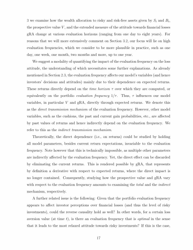
Figure 5: Prospective value evolution on the two evaluation-frequency segments.

(a) τ ≤ 1 year.

1m 2m 3m 4m 5m 6m 7m 8m 9m 10m 11m 1y0

50

100

150

200

250

300

350

400

τ

US $


(b) τ ≥ 1 year.

1y 2y 3y 4y 5y 6y 7y 8y−4000

−3000

−2000

−1000

0

1000

2000

3000

4000

τ

US $


This figure illustrates the prospective value V (in US $) from Equation (13) and its two components, thePT-effect and the cushion effect, as functions of the portfolio evaluation horizon τ . V reflects the perceivedutility of risky investments and captures the total impact of τ on investor behavior (through expectedreturns and other model variables). The PT-effect corresponds to the representation of V in PT, withoutaccounting for the influence of past performance, which is encompassed by the cushion effect. Higher V -values point to an increased utility of risky investments as perceived by non-professional investors. Panela depicts the evolution of V for evaluation horizons up to one year (in monthly increments) and panelb for evaluation horizons from one to eight years (in yearly increments). We assume myopic cushionsSt − St−1, Rt ∼ N(0, 1), Et[Rt+1] = mean

s=0,...,t[Rs], λ = 2.25, and k = 3. The sample covers 24 years of

analysis (from 03/01/1983 to 03/01/2006).

In the left segment, the perceived risky value appears to increase on average with the

evaluation horizon. In effect, the curve V (τ) in panel a of Figure 5 (panel b of Figure 10) is

acceptably well described by a polynomial of first order.37 Accordingly, the subjectively

perceived utility of the non-professional investors – captured by the prospective value

– should be maximized at the highest frequency of this domain, which is one year.38

One year can be hence designated as the optimal evaluation frequency with respect to

minimizing loss aversion and hence maximizing risky investments.

In the same spirit, the highest evaluation frequency of one day entails a minimal

expected value of the risky portfolio, pushing investors to step out of the risky market

and to allocate (almost) all their money to risk-free assets. In other words, loss-averse

investors should check the performance of their risky investments as seldom as possible

37Specifically, the adjusted R-squared yields 91.69% (77.44%) for myopic (dynamic) cushions. Theestimations are based on polynomial regression fitting performed with the Matlab Curve Fitting Toolbox.All findings in this section are robust across different parameter specifications, such as of the loss aversioncoefficient, the sensitivity to past losses, the cushion, returns distribution, expected returns, etc. Furtherresults are available upon request.

38In fact, the prospective value in the left segment in Figures 5 and 10 attains its maximum at elevenmonths. As this value lies closely to the predicted maximum point of one year and as one year is a muchmore noticeable value in investor perception, we consider one year as a sufficiently good approximationfor the optimum.

29

in order to maximize the corresponding prospective value of their investments. Under

the practical informational constraints that govern financial markets nowadays, one year

appears to be the most reasonable evaluation time that would increase the perceived

returns of risky investments.

3.3 The evolution of the actual attitude towards financial losses

In this section, we extend the analysis in the frequency domain to our new measure of

loss attitude gRA. In so doing, we study the indirect transmission mechanism mentioned

in Section 2.4. Being a derivative of a linear variable gRA does not contain any direct

influence (i.e., through the expected risk premium) of the evaluation frequency. The

variation of gRA captures thus the collateral impact of τ on other model parameters,

such as the cushion S − Z, the probability of past gains π, the probability of a positive

risk premium given past losses ω, and that of an acceptable premium given past losses ψ.

Panel a of Figure 6 (Figure 11 in Appendix 5.3) illustrates the gRA course for evalua-

tion frequencies ranging from one month to eight years and myopic (dynamic) cushions.39

On average, gRA appears to increase with the evaluation horizon, pointing to a more re-

laxed attitude towards financial losses as portfolio performance is checked less often. Note

that this occurs at all frequencies and not only in the left segment, as was the case for

the prospective value in Section 3.2.1. Thus, while the impact of the evaluation frequency

on the loss perception can be ambiguous in a context where both direct and indirect

transmission mechanisms are considered, the indirect mechanism consistently supports

the concept of mLA.

The ambiguity of the total transmission mechanism reported for the prospective value

appears to be therefore given by its direct component, i.e., through expected returns.

The cushion effect, that is highly dependent on returns, distorts the evolution of the

prospective value for very seldom portfolio checks, making it extremely sensitive to past

performance.

Similarly to the prospective value, we consider a segmentation of gRA at the evaluation

horizon of one year (see panels b and c in Figures 6 and 11). In the left segment (panels

39All findings in this section are robust across different parameter specifications. Further results areavailable upon request.

30

Figure 6: Evolution of the global first-order riskaversion for different evaluation frequencies.

(a) All evaluation frequencies.

1m 1y 2y 3y 4y 5y 6y 7y 8y0

1

2

3

4

5

6

7

8x 10

4

τ

US $

/ cha

nge (

in %

) of th

e exp

ected

risk p

remi

um

(b) τ ≤ 1 year.

1m 2m 3m 4m 5m 6m 7m 8m 9m 10m 11m 1y0.2

0.4

0.6

0.8

1

1.2

1.4

1.6

1.8

2x 10

4

τ

US

$ /

chan

ge (i

n %

) of t

he e

xpec

ted

risk

prem

ium

(c) τ ≥ 1 year.

1y 2y 3y 4y 5y 6y 7y 8y1

2

3

4

5

6

7

8x 10

4

τ

US

$ /

chan

ge (i

n %

) of t

he e

xpec

ted

risk

prem

ium

This figure illustrates the evolution of our measure of the loss attitude gRA (in US $ per percentagechange of the expected risk premium) from Equation (14) as function of the portfolio evaluation horizonτ . gRA reflects the sensitivity of the prospective value to the variation of expected returns. It capturesmerely the indirect impact of τ on investor behavior, i.e. through channels other than expected returns,such as the cushion, the probabilities of past gains and losses, etc. Higher gRA-values point to a morerelaxed loss attitude. Panel a depicts gRA for all evaluation horizons, panel b focuses on horizons up toone year (in monthly increments), and panel c on horizons from one to eight years (in yearly increments).We assume myopic cushions St − St−1, Rt ∼ N(0, 1), Et[Rt+1] = mean

s=0,...,t[Rs], λ = 2.25, and k = 3. The

sample covers 24 years of analysis (from 03/01/1983 to 03/01/2006).

31

b), simple lines appear to fit the data acceptably well.40 Our measure gRA attains its

maximum for the lowest frequency of this segment, i.e. of one year.41

As mentioned in Section 2.3, higher gRA-values represent the result of a more relaxed

attitude towards financial losses. Thus, minimizing the loss aversion – as measured by gRA

– requires again that portfolio performance should be checked as seldom as possible. For

the left segment, this is consistent with the recommendation derived from the perception

of risky investments – as captured by the prospective value – in Section 3.2.1.

In the right evaluation-frequency segment, the course of gRA is more complex, so that

second-order polynomials are necessary in order to acceptably describe the data.42 The

maximum of these parabolas is achieved at an evaluation frequency of around five years,

which might recommend this frequency as an optimal one in this segment.43 Nevertheless,

as stressed above, we consider the right segment to be of less practical importance.

In sum, both the total and the indirect mechanisms by which the evaluation frequency

impacts perceptions and decisions suggest that, under practical information constraints,

an improvement in the investors’ attitude towards risky holdings can be achieved for

yearly performance checks.

3.4 A comparison with the portfolio optimization framework

This section proposes a way to “translate” the results obtained in our framework in terms

of the portfolio optimization “language” spoken by professional managers. Specifically,

our investors individually ascertain the maximum sustainable level of losses VaR* on the

basis of subjective behavioral parameters. By contrast, in practice, managers standardize

the risk definition that could not (sufficiently) account for individual characteristics of

their clients. For instance, when risk is measured by means of the VaR concept, it can be

reduced to specific confidence levels and time horizons. In order to provide a comparison

of these two frameworks – termed in Section 2 as “endogenous” and “exogenous”, respec-

tively – we confront the VaR* in our model with the standard VaR used by portfolio

managers.

40Specifically, the adjusted R-squared yields 90.5% (91.57%) for myopic (dynamic) cushions.41A statement which is now consistent both with the data and the fitted curve.42Specifically, the adjusted R-squared yields 49.61% (60.74%) for myopic (dynamic) cushions.43Specifically, this frequency yields 4.9859 (5.3178) for myopic (dynamic) cushions.

32

In particular, we perform twofold equivalence computations: First, we start from our

VaR*-estimates and derive equivalent significance levels α from the VaR-formula. Second,

we apply confidence levels commonly used (such as 1% and 10%) to the same VaR-

formula and obtain equivalent average coefficients of loss aversion and equivalent wealth

percentages invested in the risky portfolio, on the basis of the corresponding formulas and

estimates in our model.

3.4.1 VaR*-equivalent significance levels

Portfolio managers consider the risk level indicated by their clients VaR∗ in terms of the

standard concept of VaR, specifically as VaRex. In other words, VaR* is equated with the

lower quantile of the portfolio gross returns at a given (i.e. fixed) significance level that

we denote by α∗ (or confidence 1−α∗). According to Equation (5), if the portfolio VaR at

time t corresponds to an αt > α∗ (or equivalently, to a confidence level 1− αt < 1− α∗),

then too much risk would arise by putting the entire wealth in the risky portfolio. The

portfolio manager will conclude that a percentage of the investors’ wealth should be lent

(i.e. invested in the risk-free asset) Bt < 0. On the contrary, if αt < α∗, then the portfolio

risk meets the individual risk requirements – being lower than the subjective risk threshold

– and investors borrow extra money Bt > 0 in order to increase their S&P 500-holdings.

In this section, we apply the formulas suggested by portfolio theory in order to de-

termine the significance levels that would correspond to the estimates of VaR∗t+1 derived

from Equation (11) on the basis of real market data. The corresponding averages of α∗

over time are listed in Table 2 for different portfolio evaluation frequencies, normally dis-

tributed and Student-t distributed gross returns, myopic cushions and dynamic cushions.

The results are striking: The equivalent significance level α∗ lies below the commonly

acceptable interval (being practically zero). Thus, the assumption of classical portfolio

selection models based on the VaR-concept that investors choose significance levels α in

the interval [1, 10]% appears to be at odds with the findings in our VaR*-framework,

for any evaluation frequency higher than one year. Even the lowest significance level of

1% used in standard portfolio models is not able to capture the loss aversion of non-

professional investors acting according to our setting. In other words, investors may be

substantially more risk averse in practice than actually considered in theory.

33

Table 2: Portfolio-equivalent significance levels of the estimated VaR∗t+1 (α∗).

Myopic cushions Dynamic cushionsEvaluation Portfolio returns Portfolio returnsfrequency Normal Student-t Normal Student-t


This table presents the portfolio-equivalent significance levels α∗

of the estimated VaR* from Equation (11) at different evaluationhorizons τ up to one year for both myopic cushions St − St−1

and dynamic cushions η(St − Zt−1R), and standard normal andStudent-t with 5 degrees of freedom distributed portfolio grossreturns Rt. Other parameter values used are λ = 2.25, k = 3,η = 0.9 and R = mean[Rt].

3.4.2 Portfolio-equivalent indices of loss aversion

The same equivalence issue can also be addressed from the opposite viewpoint: we de-

termine the values of λ∗t+1 in Equation (12) and the average investment in risky assets

that result from our VaR*-formula in Equation (11). These values correspond to the risk

levels used (by managers) according to the conventional VaR-procedure using common

significance levels α of 1% and 10%.

Tables 3 and 4 (Tables 7 and 8 in Appendix 5.3) present the results of this analysis for

normally distributed and Student-t distributed portfolio returns and myopic (dynamic)

cushions. Recall that the portfolio VaR in Equation (4) is estimated using a 5% signifi-

cance that is considered the benchmark for the values in these tables (i.e. it corresponds

to 100% risky investments).

Accordingly, the equivalent recommendations concerning the money to be invested

in risky assets that result from the optimal portfolio allocation under VaR at 1% (10%)

significance lie well below (above) the benchmark VaR at 5%. This points out a higher

(lower) loss aversion in our endogenous VaR*-framework – after restating it in terms of the

exogenous-VaR model – relative to the portfolio risk measured by VaR. Comparing Tables

3 and 4 (Tables 7 and 8 in Appendix 5.3), we can observe that the lower the significance

34

Table 3: Wealth percentages invested in S&P 500 and the average λ∗, for α = 1%.

Wealth % λ∗

Evaluation Portfolio returns Portfolio returnsfrequency Normal Student-t Normal Student-t


This table presents the average wealth percentages invested in therisky portfolio (first two columns) and the average loss-aversioncoefficients λ∗ from Equation (12) (last two columns) equivalentto a portfolio significance level α = 1% at different evaluationhorizons τ up to one year. The 100% level for the wealth percent-ages invested in risky assets corresponds to α = 5% and λ = 1points to a loss-neutral attitude. We assume myopic cushionsSt − St−1, standard normal and Student-t with 5 degrees of free-dom distributed portfolio gross returns Rt, λ = 2.25, and k = 3.


Wealth % λ∗



This table presents the average wealth percentages invested in therisky portfolio (first two columns) and the average loss-aversioncoefficients λ∗ from Equation (12) (last two columns) equivalentto a portfolio significance level α = 10% at different evaluationhorizons τ up to one year. The 100% level for the wealth percent-ages invested in risky assets corresponds to α = 5% and λ = 1points to a loss-neutral attitude. We assume myopic cushionsSt − St−1, standard normal and Student-t with 5 degrees of free-dom distributed portfolio gross returns Rt, λ = 2.25, and k = 3.

(or the higher the confidence level) is, the more risk averse the non-professional investors

become, as the proportion of wealth invested in the risky portfolio is smaller than 100%.

35

However, even the lowest percentages in Tables 3 and 7 are still much higher than those

in Table 1, where VaR* is treated as endogenous, mainly for high frequency revisions.

Interestingly, the results for α = 1% are qualitatively consistent with our previous

findings supporting mLA, since the wealth percentages invested in risky assets decrease

for higher evaluation frequencies, although their variation is much weaker than for the

case with α = 5% considered in Section 3.1.1. By contrast, when the confidence level

increases to α = 10%, this phenomenon is reversed and investors appear to allocate slightly

more money to the risky portfolio for more frequent evaluations. As mLA is a widely

documented phenomenon, we can conclude that the traditional portfolio optimization

framework fails once more to capture the real investor behavior in a consistent way. This

problem appears to become more acute for more relaxed assumptions regarding the risk

attitude.

Similar conclusions can be drawn with respect to the equivalent loss-aversion coefficient

λ∗ derived for conventional significance levels assumed in previous research. Its values in

Tables 3 and 4 (Tables 7 and 8 in Appendix 5.3) for myopic (dynamic) cushions are much

lower than the empirical level estimated in the original PT and largely used in previous

empirical research44 of 2.25. For the majority of the considered combinations of α-values

and evaluation frequencies, we obtain λ∗ ' 1, a level that indicates identical perception

over gains and losses according to the value function from Equation (13) (and recalling

that k = 0, i.e. no influence of past losses). Actually, this “neutral” level of 1 is exceeded

rarely for some evaluation frequencies for α = 1% and 10%. This reinforces our earlier

claim that even assuming low significance levels (e.g. α = 1% as is the common case in

previous portfolio optimization research) entails an underestimation of the loss attitude

of real investors captured by the specific coefficient λ.

4 Summary and conclusions

This paper investigates the behavior of non-professional investors facing the problems of

fixing a maximal acceptable level for financial losses and of optimally allocating wealth

between a risk-free asset and a risky portfolio. We assume that these investors are loss

44Such as Barberis, Huang, and Santos (2001) and Benartzi and Thaler (1995).

36

averse, narrowly frame financial investments, and perceive future portfolio returns as being

influenced by past portfolio performance.

We extend the portfolio allocation model developed in Campbell, Huisman, and Koedijk

(2001) in order to incorporate the effect of a desired risk level that is now subjectively

assessed (VaR*). The first task of our non-professional investors consists of fixing their

individual VaR*-level. This is subsequently communicated to professional portfolio man-

agers in charge of finding the optimal composition of the risky portfolio. Based on VaR*,

portfolio managers derive the optimal sum of money to be invested in risk-free assets.

The non-professional clients are thus provided with a recommendation of how to allocate

money between risky and risk-free assets that corresponds to their personal perceptions

and preferences.

In modeling the investors’ perception over the risky investment that yields the subjec-

tive VaR*, we employ the extended subjective valuation of prospective risky investments

proposed in Barberis, Huang, and Santos (2001) and rely on the notion of myopic loss

aversion introduced in Benartzi and Thaler (1995). The contribution of our paper is

to integrate these behavioral explanations in the portfolio decision framework mentioned

above. Moreover, we enrich the two models with original findings that stem both from the-

oretical considerations and results obtained on the basis of real market data (specifically,

the S&P 500 and the US 3-month T-bill returns).

Considering that investors are merely concerned with financial investments as a source

of utility, we build on the theoretical modelling of their perceptions of risky assets (the

value function) and define the maximum individually sustainable level of financial losses

(VaR*). This VaR*-level serves in deciding upon the optimal amount of money to be

invested in the risky portfolio. Also, we propose a way in which non-professional investors

can assess the utility of risky prospects (the prospective value). Moreover, we introduce

an extended measure, the global first-order risk aversion, that attempts to better capture

the actual attitude towards financial losses of real investors. We finally investigate how

the portfolio evaluation frequency impacts, through different mechanisms, the prospective

value and this further measure of the loss attitude. In this context, we also suggest a way

to derive the horizon of performance revisions that maximizes risky investments.

The theoretical results are supported and extended by our application. We show that,

37

in sum, our non-professional investors demonstrate myopic loss aversion. They allocate

the main part of their wealth to risk-free assets, while a smaller sum (always lower than

35% of wealth) is put into the risky portfolio. This latter sum substantially decreases at

higher frequencies at which the portfolio performance is evaluated.

Furthermore, financial wealth fluctuations determined by the success or failure of pre-

vious decisions (the cushion) exert a significant impact on the current portfolio allocation.

They make investors without substantial cushion gains firmly refuse holding a large frac-

tion of risky assets.

One year appears to be a critical evaluation frequency under practical market con-

straints, commonly used in practice, and optimal from the viewpoint of maximizing risky

holdings in consequence of a more relaxed attitude. The individual perception of risky

investments, captured by the prospective value, and the loss attitude measured by the

global first-order risk aversion can be split into two segments with qualitatively distinct

evolutions around this frequency of one year. Myopic loss aversion holds for the segment

of evaluation frequencies of at least one year that can be considered as being the only one

of practical relevance. However, the prospective value, which reflects the total impact of

the evaluation frequency, reveals a somewhat ambiguous behavior when portfolio perfor-

mance is checked at time intervals longer than one year. This is apparently due to the

direct component of this total impact (i.e. the manifestation through expected returns),

since the indirect component, that can be measured by means of the global first-order risk

aversion, shows a more consistent evolution across all analyzed evaluation frequencies.

Finally, the estimation of variables aimed at establishing an equivalence between the

theoretical portfolio optimization under exogenous VaR-constraints and our extended

framework with individual VaR* (such as significance levels, loss aversion coefficients, and

investments in risky assets) suggests an underestimation of the attitude of non-professional

investors towards financial losses.

38

5 Appendix

5.1 Expectation and variance of the loss utility

According to Equations (8) and (9), we have:

Et[loss-valuet+1] = πt(1− ψt)(λStEt[xt+1] + (λ− 1)(St − Zt)Rft)

+ (1− πt)(1− ωt)(λStEt[xt+1]− k(St − Zt)Et[xt+1])

=cond.

λStEt[xt+1] +(πt(1− ψt)((λ− 1)Rft + kEt[xt+1])− kEt[xt+1]

)(St − Zt).

(15)

Also, the expectation of the squared loss value and consequently the loss variance result

in:

Et[loss-value2t+1] = πt(1− ψt)(λStEt[xt+1] + (λ− 1)(St − Zt)Rft)

2

+ (1− πt)(1− ωt)(λStEt[xt+1]− k(St − Zt)Et[xt+1])2

= (λStEt[xt+1])2 +

(πt(1− ψt)((λ− 1)2R2

ft − k2x2t+1) + k2x2

t+1

)(St − Zt)

2

+ 2(πt(1− ψt)((λ− 1)Rft + kEt[xt+1])− kEt[xt+1]

)λStEt[xt+1](St − Zt),

and

V art[loss-valuet+1] = Et[loss-value2t+1]− E2

t [loss-valuet+1]

= πt(1− ψt)(1− πt(1− ψt)

)((λ− 1)Rft + kEt[xt+1]

)2

(St − Zt)2.

(16)

The variance of the loss value is exclusively based on past performance, being generated

only by the cushion St − Zt.

39

5.2 Descriptive statistics

Table 5: Log-difference of the S&P 500 index.

S&P 500Evaluation frequency

Quarterly YearlyMean 0.017 0.066

Median 0.018 0.071Std.Dev. 0.079 0.136Kurtosis 2.661 -0.9659Skewness -0.671 -0.205

Max. 0.290 0.345Min. -0.302 -0.207Obs. 175 43

This table presents descriptive statistics ofthe log-difference Rt of the S&P 500 indexfor quarterly and yearly portfolio evaluations,corrected for dividends and stock splits. Thisindex is used as proxy for the risky invest-ment. The data series range from 01/02/1962to 03/09/2006.

40

Table 6: 3-month T-bill log-returns.

3-month T-billEvaluation frequencyQuarterly Yearly

Mean 0.017 0.073Median 0.017 0.070Std.Dev. 0.006 0.026Kurtosis 0.623 0.974Skewness 0.951 1.042

Max. 0.036 0.142Min. 0.009 0.037Obs. 175 43

This table presents descriptive statistics of the 3-month T-bill log-returns Rf for quarterly and yearlyportfolio evaluations, corrected for dividends andstock splits. This index is used as proxy for therisk-free investment. The data series range from01/02/1962 to 03/09/2006.

5.3 Results for the dynamic cushion

41

Figure 7: Evolution of risky returns, dynamic cushions, and wealth per-centages invested in the risky portfolio for yearly portfolio evaluations.

(a) Yearly S&P 500 log-returns.

82 83 84 85 86 87 88 89 90 91 92 93 94 95 96 97 98 99 00 01 02 03 04 05 06−0.2

−0.1

0

0.1

0.2

0.3

0.4

year

retur

ns

(b) Yearly dynamic cushions.

82 83 84 85 86 87 88 89 90 91 92 93 94 95 96 97 98 99 00 01 02 03 04 05 06−6000

−5000

−4000

−3000

−2000

−1000

0

1000

2000

3000

4000

5000

year

US $

(c) Yearly wealth percentage invested in S&P 500.

82 83 84 85 86 87 88 89 90 91 92 93 94 95 96 97 98 99 00 01 02 03 04 05 0610

15

20

25

30

35

40

45

50

55

year

wealt

h per

centa

ge

This figure illustrates the annual log-returns Rt of the index S&P 500, the corresponding yearly evolution(in US $) of the past performance encompassed by the dynamic cushions η(St−Zt−1R), and the resultingyearly wealth percentages St/Wt invested in the risky portfolio. The wealth percentages are obtained fromEquation (5), where VaRex is replaced by the VaR*-values from Equation (11) and the risky investmentSt results from Equation (6). We assume Rt ∼ N(0, 1), Et[Rt+1] = mean

s=0,...,t[Rs], λ = 2.25, k = 3,

R = mean[Rt], and η = 0.9. The sample covers 24 years of analysis (from 03/01/1983 to 03/01/2006),such that every point on the horizontal time axis corresponds to 1st March of each year.

42

Figure 8: Evolution of risky returns, dynamic cushions, and percent-ages invested in the risky portfolio for daily portfolio evaluations.

(a) Daily S&P 500 returns.

82 83 84 85 86 87 88 89 90 91 92 93 94 95 96 97 98 99 00 01 02 03 04 05 06−0.1

−0.08

−0.06

−0.04

−0.02

0

0.02

0.04

0.06

0.08

0.1

year

retu

rns

(b) Daily dynamic cushions.

82 83 84 85 86 87 88 89 90 91 92 93 94 95 96 97 98 99 00 01 02 03 04 05 06−50

−40

−30

−20

−10

0

10

20

30

40

50

year

US $

(c) Daily percentage investments in S&P 500.

82 83 84 85 86 87 88 89 90 91 92 93 94 95 96 97 98 99 00 01 02 03 04 05 060

5

10

15

20

25

30

35

40

45

50

year

wealt

h per

centa

ge

This figure illustrates the daily log-returns Rt of the index S&P 500, the corresponding daily past per-formance (in US $) encompassed by the dynamic cushions η(St −Zt−1R), and the resulting daily wealthpercentages St/Wt invested in the risky portfolio. The wealth percentages are obtained from Equation(5), where VaRex is replaced by the VaR*-values from Equation (11) and the risky investment St resultsfrom Equation (6). We assume Rt ∼ N(0, 1), Et[Rt+1] = mean

s=0,...,t[Rs], λ = 2.25, k = 3, R = mean[Rt],

and η = 0.9. The sample covers 24 years of analysis (from 03/01/1983 to 03/01/2006), such that everypoint on the horizontal time axis corresponds to 1st March of each year.

43

Figure 9: Prospective value evolution for yearly and daily evaluations.

(a) Yearly evaluations.

82 83 84 85 86 87 88 89 90 91 92 93 94 95 96 97 98 99 00 01 02 03 04 05 06−1500

−1000

−500

0

500

1000

1500

year

US $


(b) Daily evaluations.

82 83 84 85 86 87 88 89 90 91 92 93 94 95 96 97 98 99 00 01 02 03 04 05 06−15

−10

−5

0

5

10

15

year

US $


This figure illustrates the yearly and daily evolution of the prospective value V (in US $) from Equation(13) and of its two components, the PT-effect and the cushion effect, that correspond to the two termsin this equation. The PT-effect corresponds to the representation of V in PT, without accounting for theinfluence of past performance, which is encompassed by the cushion effect. We assume dynamic cushionsη(St − Zt−1R), Rt ∼ N(0, 1), Et[Rt+1] = mean

s=0,...,t[Rs], λ = 2.25, k = 3, R = mean[Rt], and η = 0.9.

The sample covers 24 years of analysis (from 03/01/1983 to 03/01/2006), such that every point on thehorizontal time axis corresponds to 1st March of each year.

44

Figure 10: Prospective value evolution in for different evaluation frequencies.

(a) All frequencies.

1m 1y 2y 3y 4y 5y 6y 7y 8y−7000

−6000

−5000

−4000

−3000

−2000

−1000

0

1000

2000

3000

evaluation frequency

US $


(b) τ ≤ 1 year.

1m 2m 3m 4m 5m 6m 7m 8m 9m 10m 11m 1y−20

0

20

40

60

80

100

120

140

160

180


US

$


(c) τ ≥ 1 year.

1y 2y 3y 4y 5y 6y 7y 8y−7000

−6000

−5000

−4000

−3000

−2000

−1000

0

1000

2000

3000


US

$


This figure illustrates the prospective value V (in US $) from Equation (13) and its two components,the PT-effect and the cushion effect, as functions of the portfolio evaluation horizon τ . V reflects theperceived utility of risky investments and captures the total impact of τ on investor behavior (throughexpected returns and other model variables). The PT-effect corresponds to the representation of V inPT, without accounting for the influence of past performance, which is encompassed by the cushioneffect. Higher V -values point to an increased utility of risky investments as perceived by non-professionalinvestors. Panel a depicts the evolution of V for all evaluation horizons, panel b focuses on horizons up toone year (in monthly increments), and panel c on horizons from one to eight years (in yearly increments).We assume dynamic cushions η(Zt−1R + St), Rt ∼ N(0, 1), Et[Rt+1] = mean

s=0,...,t[Rs], λ = 2.25, k = 3,

R = mean[Rt], and η = 0.9. The sample covers 24 years of analysis (from 03/01/1983 to 03/01/2006).

45

Figure 11: Evolution of the global first-orderrisk aversion for different evaluation frequencies.

(a) All evaluation frequencies.

1m 1y 2y 3y 4y 5y 6y 7y 8y0

0.5

1

1.5

2

2.5

3

3.5

4

4.5

5x 10

4

τ

US $

/ cha

nge

(in %

) of th

e exp

ected

risk p

remi

um

(b) τ ≤ 1 year.

1m 2m 3m 4m 5m 6m 7m 8m 9m 10m 11m 1y0.2

0.4

0.6

0.8

1

1.2

1.4

1.6

1.8x 10

4

τ

US

$ /

chan

ge (i

n %

) of t

he e

xpec

ted

risk

prem

ium

(c) τ ≥ 1 year.

1y 2y 3y 4y 5y 6y 7y 8y1.5

2

2.5

3

3.5

4

4.5

5x 10

4

τ

US

$ /

chan

ge (i

n %

) of t

he e

xpec

ted

risk

prem

ium

This figure illustrates the evolution of our measure of the loss attitude gRA (in US $ per percentagechange of the expected risk premium) from Equation (14) as function of the portfolio evaluation horizonτ . gRA reflects the sensitivity of the prospective value to the variation of expected returns. It capturesmerely the indirect impact of τ on investor behavior, i.e. through channels other than expected returns,such as the cushion, the probabilities of past gains and losses, etc. Higher gRA-values point to a morerelaxed loss attitude. Panel a depicts gRA for all evaluation horizons, panel b focuses on horizons up toone year (in monthly increments), and panel c on horizons from one to eight years (in yearly increments).We assume dynamic cushions η(Zt−1R + St), Rt ∼ N(0, 1), Et[Rt+1] = mean

s=0,...,t[Rs], λ = 2.25, k = 3,

R = mean[Rt], and η = 0.9. The sample covers 24 years of analysis (from 03/01/1983 to 03/01/2006).

46


Wealth % λ∗



This table presents the average wealth percentages invested in therisky portfolio (first two columns) and the average loss-aversioncoefficients λ∗ from Equation (12) (last two columns) equivalentto a portfolio significance level α = 1% at different evaluationhorizons τ up to one year. The 100% level for the wealth percent-ages invested in risky assets corresponds to α = 5% and λ = 1points to a loss-neutral attitude. We assume dynamic cushionsη(St − Zt−1R), standard normal and Student-t with 5 degrees offreedom distributed portfolio gross returns Rt, λ = 2.25, k = 3,R = mean[Rt], and η = 0.9.

47


Wealth % λ∗



This table presents the average wealth percentages invested in therisky portfolio (first two columns) and the average loss-aversioncoefficients λ∗ from Equation (12) (last two columns) equivalentto a portfolio significance level α = 10% at different evaluationhorizons τ up to one year. The 100% level for the wealth percent-ages invested in risky assets corresponds to α = 5% and λ = 1points to a loss-neutral attitude. We assume dynamic cushionsη(St − Zt−1R), standard normal and Student-t with 5 degrees offreedom distributed portfolio gross returns Rt, λ = 2.25, k = 3,R = mean[Rt], and η = 0.9.

48

References

Artzner, P., F. Delbaen, J. Eber, and D. Heath (1999): “Coherent Measures of

Risk,” Mathematical Finance, 9, 203–228.

Barberis, N., and M. Huang (2004): “Preferences with Frames: A New Utility Specifi-

cation that Allows for the Framing of Risks,” Working paper, University of Chicago,

Stanford University.

(2006): “The Loss Aversion/Narrow Framing Approach to Stock Market Pricing

and Participation Puzzles,” NBER Working paper No. 12378.

Barberis, N., M. Huang, and T. Santos (2001): “Prospect Theory and Asset

Prices,” Quarterly Journal of Economics, 116, 1–53.

Basak, S., and A. Shapiro (2001): “Value-at-Risk-Based Risk Management: Optimal

Policies and Asset Prices,” Review of Financial Studies, 14.

Benartzi, S., and R. H. Thaler (1995): “Myopic Loss Aversion and the Equity

Premium Puzzle,” Quarterly Journal of Economics, 110, 73–92.

Berkelaar, A., and R. Kouwenberg (2006): “From Boom ’til Bust: How Loss

Aversion Affects Asset Prices,” Working Paper, unpubl.

Berkelaar, A. B., R. Kouwenberg, and T. Post (2004): “Optimal Portfolio Choice

under Loss Aversion,” Review of Economics and Statistics, 86, 973987.

Campbell, R., R. Huisman, and K. Koedijk (2001): “Optimal Portfolio Selection

in a Value-at-Risk Framework,” Journal of Banking and Finance, 25, 1789–1804.

Embrechts, P., A. McNeil, and D. Straumann (1999): “Correlation and

Dependance in Risk Management: Properties and Pitfalls,” Available from

www.defaultrisk.com.

Gneezy, U., A. Kapteyn, and J. Potters (2003): “Evaluation Periods and Asset

Price in a Market Experiment,” Journal of Finance, 58, 821–837.

Gneezy, U., and J. Potters (1997): “An Experiment on Risk Taking and Evaluation

Periods,” Quarterly Journal of Economics, 102, 631–645.

49

Haigh, M. S., and J. A. List (2005): “Do Professional Traders Exhibit Myopic Loss

Aversion? An Experimental Analysis,” Journal of Finance, 60, 523–534.

Kahneman, D., and A. Tversky (1979): “Prospect Theory: An Ananlysis of Decision

Under Risk,” Econometrica, 47, 263–291.

Rockafellar, R., and S. Uryasev (2000): “Optimization of Conditional Value-At-

Risk,” The Journal of Risk, 2, 21–41.

Szego, G. (2002): “Measures of Risk,” Journal of Banking and Finance, 26, 1253–1272.

Thaler, R. H., A. Tversky, D. Kahneman, and A. Schwartz (1997a): “The Ef-

fect of Myopia and Loss Aversion on Risk Taking,” Quarterly Journal of Economics,

102, 647–661.

(1997b): “The effect of myopia and loss aversion on risk taking,” Quarterly

Journal of Economics, 102(2), 647–661.

Tversky, A., and D. Kahneman (1992): “Advances in Prospect Theory: Cumulative

Representation of Uncertainty,” Journal of Risk and Uncertainty, 4(5), 297–323.

50

Fordham University Department of Economics Discussion ... · Fordham University Department of...

Documents

Transcript of Fordham University Department of Economics Discussion ... · Fordham University Department of...