Forcasting- Seasonal Index Number 26, 27, 28,29, 30 page · PDF file ·...
13
[Type text] Assigment November 9 th Forcasting- Seasonal Index Number 26, 27, 28,29, 30 page 630-631 Statistical Techniques in Business and Economics Lind/Marchal/ Wathen
Transcript of Forcasting- Seasonal Index Number 26, 27, 28,29, 30 page · PDF file ·...

[Type text]
Assigment November 9th
Forcasting- Seasonal Index
Number 26, 27, 28,29, 30 page 630-631
Statistical Techniques in Business and Economics
Lind/Marchal/ Wathen
[Type text]
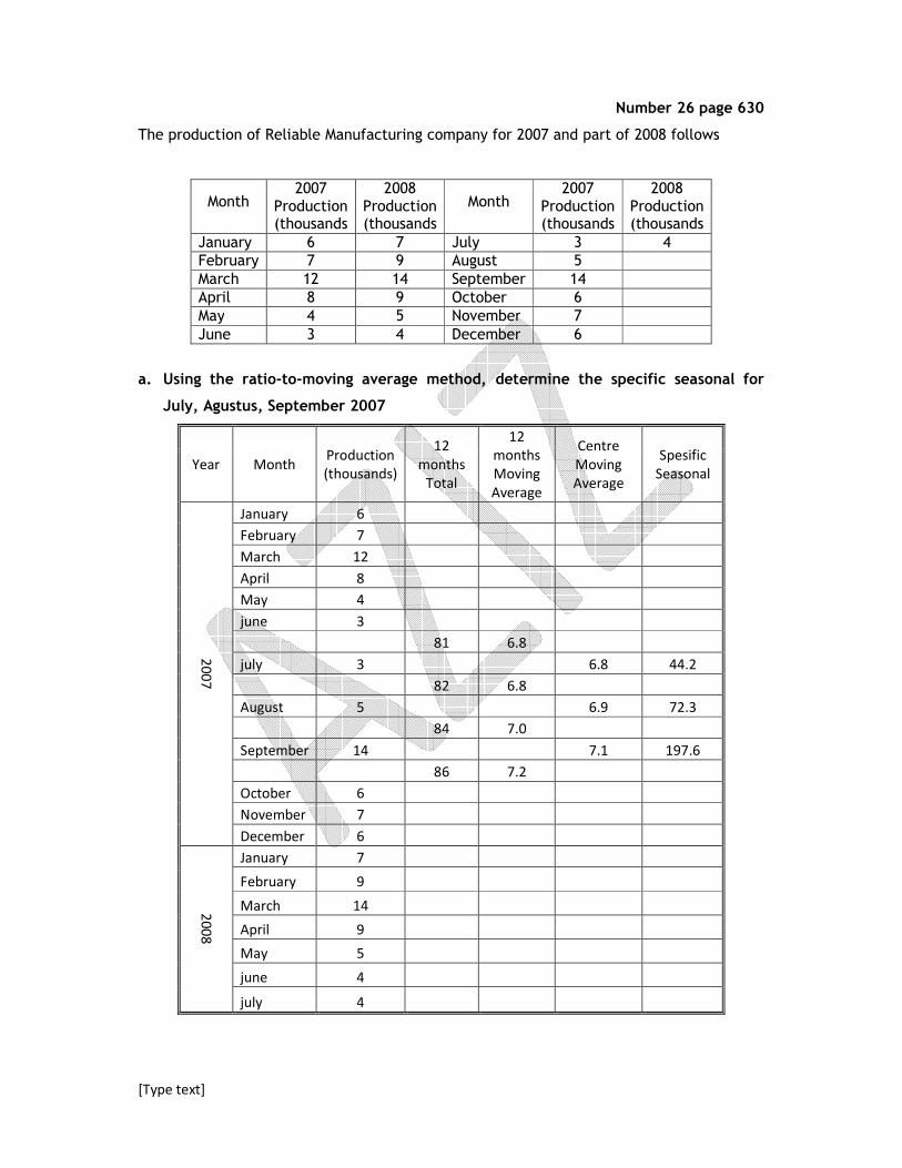
Number 26 page 630
The production of Reliable Manufacturing company for 2007 and part of 2008 follows
Month 2007
Production (thousands
2008 Production (thousands
Month 2007
Production (thousands
2008 Production (thousands
January 6 7 July 3 4 February 7 9 August 5 March 12 14 September 14 April 8 9 October 6 May 4 5 November 7 June 3 4 December 6
a. Using the ratio-to-moving average method, determine the specific seasonal for
July, Agustus, September 2007
Year Month Production
(thousands)
12
months
Total
12
months
Moving
Average
Centre
Moving
Average
Spesific
Seasonal
20
07
January 6
February 7
March 12
April 8
May 4
june 3
81 6.8
july 3 6.8 44.2
82 6.8
August 5 6.9 72.3
84 7.0
September 14 7.1 197.6
86 7.2
October 6
November 7
December 6
20
08
January 7
February 9
March 14
April 9
May 5
june 4
july 4
[Type text]
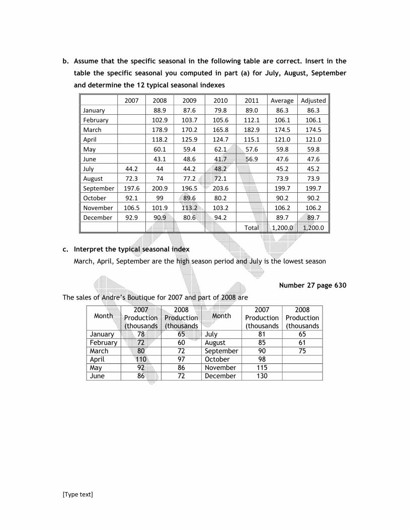
b. Assume that the specific seasonal in the following table are correct. Insert in the
table the specific seasonal you computed in part (a) for July, August, September
and determine the 12 typical seasonal indexes
2007 2008 2009 2010 2011 Average Adjusted
January 88.9 87.6 79.8 89.0 86.3 86.3
February 102.9 103.7 105.6 112.1 106.1 106.1
March 178.9 170.2 165.8 182.9 174.5 174.5
April 118.2 125.9 124.7 115.1 121.0 121.0
May 60.1 59.4 62.1 57.6 59.8 59.8
June 43.1 48.6 41.7 56.9 47.6 47.6
July 44.2 44 44.2 48.2 45.2 45.2
August 72.3 74 77.2 72.1 73.9 73.9
September 197.6 200.9 196.5 203.6 199.7 199.7
October 92.1 99 89.6 80.2 90.2 90.2
November 106.5 101.9 113.2 103.2 106.2 106.2
December 92.9 90.9 80.6 94.2 89.7 89.7
Total 1,200.0 1,200.0
c. Interpret the typical seasonal index
March, April, September are the high season period and July is the lowest season
Number 27 page 630
The sales of Andre’s Boutique for 2007 and part of 2008 are
Month 2007
Production (thousands
2008 Production (thousands
Month 2007
Production (thousands
2008 Production (thousands
January 78 65 July 81 65 February 72 60 August 85 61 March 80 72 September 90 75 April 110 97 October 98 May 92 86 November 115 June 86 72 December 130
[Type text]
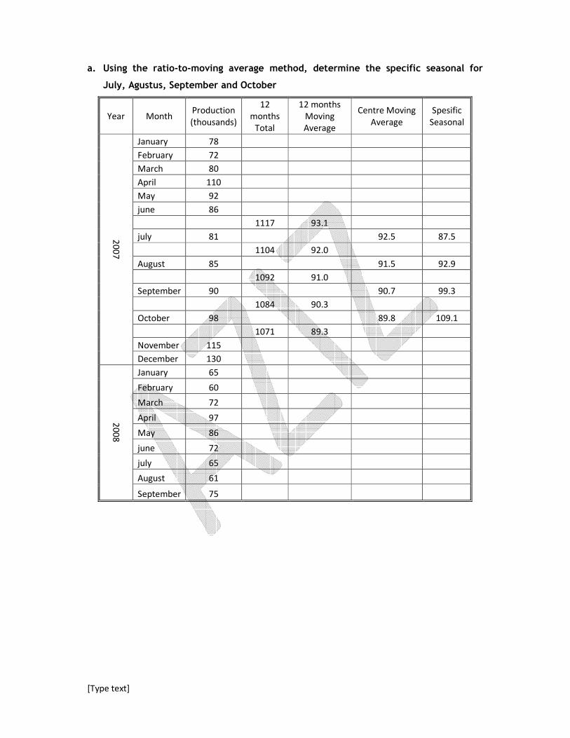
a. Using the ratio-to-moving average method, determine the specific seasonal for
July, Agustus, September and October
Year Month Production
(thousands)
12
months
Total
12 months
Moving
Average
Centre Moving
Average
Spesific
Seasonal
20
07
January 78
February 72
March 80
April 110
May 92
june 86
1117 93.1
july 81 92.5 87.5
1104 92.0
August 85 91.5 92.9
1092 91.0
September 90 90.7 99.3
1084 90.3
October 98 89.8 109.1
1071 89.3
November 115
December 130
20
08
January 65
February 60
March 72
April 97
May 86
june 72
july 65
August 61
September 75

[Type text]
b. Assume that the specific seasonal in the following table are correct. Insert in the
table the specific seasonal you computed in part (a) for July, August, September
and October and determine the 12 typical seasonal indexes
2007 2008 2009 2010 2011 Average Adjusted
January 83.9 86.7 85.6 77.3 83.4 82.9
February 77.6 72.9 65.8 81.2 74.4 74.0
March 86.1 86.2 89.2 85.8 86.8 86.4
April 118.7 121.3 125.6 115.7 120.3 119.7
May 99.7 96.6 99.6 100.3 99.1 98.5
June 92 92 94.4 89.7 92.0 91.6
July 87.5 87 85.5 88.9 87.2 86.8
August 92.9 91.4 93.6 90.2 92.0 91.6
September 99.3 97.3 98.2 100.2 98.8 98.2
October 109.1 105.4 103.2 102.7 105.1 104.6
November 123.6 124.9 126.1 121.6 124.1 123.4
December 150.9 140.1 141.7 139.6 143.1 142.3
Total 1,206.2 1,200.0
c. Interpret the typical seasonal index
April, November and December are the high season and February are the lowest season
Number 28 page 631
The quarterly production of pine lumber, in millions of board feet, by Northwest Lumber
since 2004 is
Year Winter Spring Summer Fall
2004 7.8 10.2 14.7 9.3 2005 6.9 11.6 17.5 9.3 2006 8.9 9.7 15.3 10.1 2007 10.7 12.4 16.8 10.7 2008 9.2 13.6 17.1 10.3
a. Determine the typical seasonal pattern for the production data using the ratio-
moving average

[Type text]
Year Month Production
(thousands)
Four
Quarter
Total
Four Quarter
Moving
average
Centre
Moving
Average
Spesific
Seasonal
2004
Winter 7.8
Spring 10.2
42 10.500
Summer 14.7 10.388 1.415
41.1 10.275
Fall 9.3 10.450 0.890
42.5 10.625
2005
Winter 6.9 10.975 0.629
45.3 11.325
Spring 11.6 11.325 1.024
45.3 11.325
Summer 17.5 11.575 1.512
47.3 11.825
Fall 9.3 11.588 0.803
45.4 11.350
2006
Winter 8.9 11.075 0.804
43.2 10.800
Spring 9.7 10.900 0.890
44 11.000
Summer 15.3 11.225 1.363
45.8 11.450
Fall 10.1 11.788 0.857
48.5 12.125
2007
Winter 10.7 12.313 0.869
50 12.500
Spring 12.4 12.575 0.986
50.6 12.650
Summer 16.8 12.463 1.348
49.1 12.275
Fall 10.7 12.425 0.861
50.3 12.575
2008
Winter 9.2 12.613 0.729
50.6 12.650
Spring 13.6 12.600 1.079
50.2 12.550
Summer 17.1
Fall 10.3

[Type text]
Year Winter Spring Summer Fall
2004 1.415 0.890 2005 0.629 1.024 1.512 0.803 2006 0.804 0.890 1.363 0.857 2007 0.869 0.986 1.348 0.861 2008 0.729 1.079 Average 0.758 0.995 1.410 0.853 Adjusted 0.755 0.991 1.404 0.849
b. Interpret the pattern
Demand and production pine lumber will be high at Summer.
c. Deseasonalize the data and determine the linear trend equation
∑∑
∑ ∑ ∑
==
= = =
−
−
=n
i
i
n
i
i
n
i
n
i
n
i
iiii
ttn
ytytn
b
1
2
1
2
1 1 1
)(
))((
, dan n
tby
a
n
i
n
i
ii∑ ∑= =
−
=1 1
� ��� ��.��.���� ���.���
� �� ������� � 0.14 (see Table below)
� �232.155 � 0.14�210�
20� 10.11
Year Month Production
(thousands) Index
Deseasonalized
Production (Y) Code (t) Yt t^2
2004
Winter 7.8 0.755 10.331 1 10.331 1
Spring 10.2 0.991 10.293 2 20.585 4
Summer 14.7 1.404 10.470 3 31.410 9
Fall 9.3 0.849 10.954 4 43.816 16
2005
Winter 6.9 0.755 9.139 5 45.695 25
Spring 11.6 0.991 11.705 6 70.232 36
Summer 17.5 1.404 12.464 7 87.251 49
Fall 9.3 0.849 10.954 8 87.633 64
2006
Winter 8.9 0.755 11.788 9 106.093 81
Spring 9.7 0.991 9.788 10 97.881 100
Summer 15.3 1.404 10.897 11 119.872 121
Fall 10.1 0.849 11.896 12 142.756 144
2007
Winter 10.7 0.755 14.172 13 184.238 169
Spring 12.4 0.991 12.513 14 175.177 196
Summer 16.8 1.404 11.966 15 179.487 225
Fall 10.7 0.849 12.603 16 201.649 256
2008
Winter 9.2 0.755 12.185 17 207.152 289
Spring 13.6 0.991 13.724 18 247.023 324
Summer 17.1 1.404 12.179 19 231.410 361
Fall 10.3 0.849 12.132 20 242.638 400
Toatl 232.155 210 2,532.331 2870
[Type text]
�� � 10.11 � 0.14 �
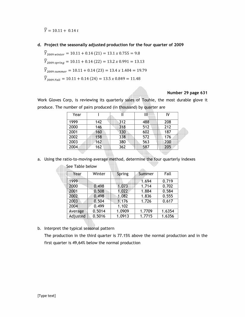
d. Project the seasonally adjusted production for the four quarter of 2009
������ ��� !" � 10.11 � 0.14 �21� � 13.1 # 0.755 � 9.8
������ '("��) � 10.11 � 0.14 �22� � 13.2 # 0.991 � 13.13
������ '*++!" � 10.11 � 0.14 �23� � 13.4 # 1.404 � 19.79
������ ,-.. � 10.11 � 0.14 �24� � 13.5 # 0.849 � 11.48
Number 29 page 631
Work Gloves Corp, is reviewing its quarterly sales of Touhie, the most durable glove it
produce. The number of pairs produced (in thousand) by quarter are
Year I II III IV
1999 142 312 488 208 2000 146 318 512 212 2001 160 330 602 187 2002 158 338 572 176 2003 162 380 563 200 2004 162 362 587 205
a. Using the ratio-to-moving-average method, determine the four quarterly indexes
See Table below
Year Winter Spring Summer Fall
1999 1.694 0.719 2000 0.498 1.073 1.714 0.702 2001 0.508 1.022 1.884 0.584 2002 0.498 1.082 1.836 0.555 2003 0.504 1.176 1.726 0.617 2004 0.499 1.102 Average 0.5014 1.0909 1.7709 1.6354 Adjusted 0.5016 1.0913 1.7715 1.6356
b. Interpret the typical seasonal pattern
The production in the third quarter is 77.15% above the normal production and in the
first quarter is 49,64% below the normal production

[Type text]
Year Month Production
(thousands)
Four
Quarter
Total
Four
Quarter
Moving
average
Centre
Moving
Average
Spesific
Seasonal
1999
Winter 142
Spring 312
1150 287.500
Summer 488 288.000 1.694
1154 288.500
Fall 208 289.250 0.719
1160 290.000
2000
Winter 146 293.000 0.498
1184 296.000
Spring 318 296.500 1.073
1188 297.000
Summer 512 298.750 1.714
1202 300.500
Fall 212 302.000 0.702
1214 303.500
2001
Winter 160 314.750 0.508
1304 326.000
Spring 330 322.875 1.022
1279 319.750
Summer 602 319.500 1.884
1277 319.250
Fall 187 320.250 0.584
1285 321.250
2002
Winter 158 317.500 0.498
1255 313.750
Spring 338 312.375 1.082
1244 311.000
Summer 572 311.500 1.836
1248 312.000
Fall 176 317.250 0.555
1290 322.500
2003
Winter 162 321.375 0.504
1281 320.250
Spring 380 323.250 1.176
1305 326.250
Summer 563 326.250 1.726
1305 326.250
Fall 200 324.000 0.617
1287 321.750
2004
Winter 162 163.875 0.989
1311 327.750
Spring 362 328.375 1.102
1316 329.000
Summer 587
Fall 205

[Type text]
Number 30 page 631
Sales of roof material, by quarter, sice 2000 by Carolina Home construction, Inc., are
shown below (in $000)
Year I II III IV
2000 210 180 60 246 2001 214 216 82 230 2002 246 228 91 280 2003 258 250 113 298 2004 249 267 116 304 2005 302 290 114 310 2006 321 291 120 320
a. Determine the typical seasonal patterns for sales using he ratio-moving average
method
Year Month Production
(thousands)
Four
Quarter
Total
Four Quarter
Moving average
Centre
Moving
Average
Spesific
Seasonal
2000
i 210
ii 180
696 174.000
iii 60 174.500 0.344
700 175.000
iv 246 179.500 1.370
736 184.000
2001
i 214 186.750 1.146
758 189.500
ii 216 187.500 1.152
742 185.500
iii 82 189.500 0.433
774 193.500
iv 230 195.000 1.179
786 196.500
2002
i 246 197.625 1.245
795 198.750
ii 228 205.000 1.112
845 211.250
iii 91 212.750 0.428
857 214.250
iv 280 217.000 1.290
879 219.750
2003
i 258 222.500 1.160
901 225.250
ii 250 227.500 1.099
919 229.750
iii 113 232.375 0.486
940 235.000
iv 298 237.125 1.257
957 239.250

[Type text]
Year Month Production
(thousands)
Four
Quarter
Total
Four Quarter
Moving average
Centre
Moving
Average
Spesific
Seasonal
2004
i 279 239.625 1.164
960 240.000
ii 267 240.750 1.109
966 241.500
iii 116 244.375 0.475
989 247.250
iv 304 250.125 1.215
1012 253.000
2005
i 302 267.250 1.130
1126 281.500
ii 290 267.750 1.083
1016 254.000
iii 114 256.375 0.445
1035 258.750
iv 310 258.875 1.197
1036 259.000
2006
i 321 130.250 2.464
1042 260.500
ii 291 300.500 0.968
1362 340.500
iii 120
iv 320
2000 2001 2002 2003 2004 2005 2006 Average Adjusment
I 1.146 1.245 1.160 1.164 1.130 2.464 1.385 1.332
II 1.152 1.112 1.099 1.109 1.083 0.968 1.087 1.046
III 0.344 0.433 0.428 0.486 0.475 0.445 0.435 0.418
IV 1.370 1.179 1.290 1.257 1.215 1.197 1.252 1.204
4.159 4.000
b. Deseasonalize the data and determine the trend equation
∑∑
∑ ∑ ∑
==
= = =
−
−
=n
i
i
n
i
i
n
i
n
i
n
i
iiii
ttn
ytytn
b
1
2
1
2
1 1 1
)(
))((
, dan n
tby
a
n
i
n
i
ii∑ ∑= =
−
=1 1
� �28 �48.078.080� � �210��4.230.148�
28�2870� � �210��� 12.63
� � 4.230.148 � 12.63�210�
28� 56.37
�� � 56.37 � 12.63 �
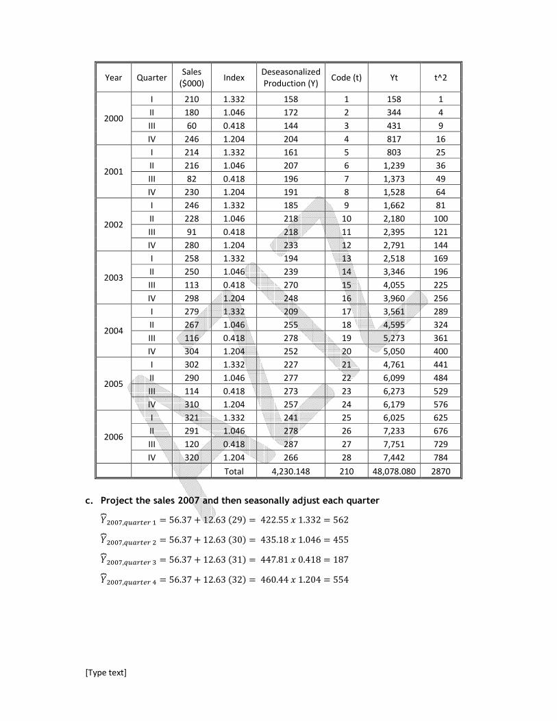
[Type text]
Year Quarter Sales
($000) Index
Deseasonalized
Production (Y) Code (t) Yt t^2
2000
I 210 1.332 158 1 158 1
II 180 1.046 172 2 344 4
III 60 0.418 144 3 431 9
IV 246 1.204 204 4 817 16
2001
I 214 1.332 161 5 803 25
II 216 1.046 207 6 1,239 36
III 82 0.418 196 7 1,373 49
IV 230 1.204 191 8 1,528 64
2002
I 246 1.332 185 9 1,662 81
II 228 1.046 218 10 2,180 100
III 91 0.418 218 11 2,395 121
IV 280 1.204 233 12 2,791 144
2003
I 258 1.332 194 13 2,518 169
II 250 1.046 239 14 3,346 196
III 113 0.418 270 15 4,055 225
IV 298 1.204 248 16 3,960 256
2004
I 279 1.332 209 17 3,561 289
II 267 1.046 255 18 4,595 324
III 116 0.418 278 19 5,273 361
IV 304 1.204 252 20 5,050 400
2005
I 302 1.332 227 21 4,761 441
II 290 1.046 277 22 6,099 484
III 114 0.418 273 23 6,273 529
IV 310 1.204 257 24 6,179 576
2006
I 321 1.332 241 25 6,025 625
II 291 1.046 278 26 7,233 676
III 120 0.418 287 27 7,751 729
IV 320 1.204 266 28 7,442 784
Total 4,230.148 210 48,078.080 2870
c. Project the sales 2007 and then seasonally adjust each quarter
������,1*-" !" � 56.37 � 12.63 �29� � 422.55 # 1.332 � 562
������,1*-" !" � � 56.37 � 12.63 �30� � 435.18 # 1.046 � 455
������,1*-" !" � 56.37 � 12.63 �31� � 447.81 # 0.418 � 187
������,1*-" !" 2 � 56.37 � 12.63 �32� � 460.44 # 1.204 � 554

[Type text]