for the Euler Equations - ntrs.nasa.gov · for the Euler Equations ... 2.8 Diagonal Dominance in...

Development of Upwind Schemes for the Euler Equations

Sukumar R. Chakravarthy

https://ntrs.nasa.gov/search.jsp?R=19870005755 2018-06-20T08:27:33+00:00Z

NASA Contractor Report 4043

Development of Upwind Schemes for the Euler Equations

Sukumar R. Chakravarthy Roc&weZZ International Science Center Thousand Oaks, California

Prepared for Langley Research Center under Contract NAS1-17492

National Aeronautics and Space Administration

Scientific and Technical Information Branch

1987

CONTENTS

Page I

1.0 INTRODUCTION . . . . . . . . . . . . . . . . . . . . . . . . . . 1

2.0 TVD FORMULATIONS OF UPWIND SCHEMES . . . . . . . . . . . 3

2.1 Summary . . . . . . . . . . . . . . . . . . . . . . . . . . . 3 I I 2.2 Introduction . . . . . . . . . . . . . . . . . . . . . . . . . . 4

1 2.3 Operational Unification of Upwind Schemes . . . . . . . . . . . . 5

2.3.1 Godunov Scheme . . . . . . . . . . . . . . . . . . . . 6 2.3.2 Osher's Scheme . . . . . . . . . . . . . . . . . . . . . 10 2.3.3 Roe's Scheme . . . . . . . . . . . . . . . . . . . . . . 11 2.3.4 Split-Flux Scheme . . . . . . . . . . . . . . . . . . . . 12 2.3.5 Second-Order Accuracy . . . . . . . . . . . . . . . . . 13 2.3.6 Summary . . . . . . . . . . . . . . . . . . . . . . . 15

2.4 TVD Scbeme Design by Preprocessing . . . . . . . . . . . . . . . 15 I 2.5 Application to General Control Volumes 17 . . . . . . . . . . . . . .

2.6 Removing Expansion Shocks 21 I

. . . . . . . . . . . . . . . . . . . 2.7 Nonlinear Stability of TVD Schemes . . . . . . . . . . . . . . . 22

2.8 Diagonal Dominance in TVD Formulations . . . . . . . . . . . . . 24

2.9 Remarks . . . . . . . . . . . . . . . . . . . . . . . . . . . . 27

3.0 RELAXATION METHODS FOR IMPLICIT UPWIND SCHEMES . . . . 29

3.1 Summary . . . . . . . . . . . . . . . . . . . . . . . . . . . 29

3.2 Introduction . . . . . . . . . . . . . . . . . . . . . . . . . . 29

3.3 Linear Scalar Equations . . . . . . . . . . . . . . . . . . . . . 30

3.3.1 Diagonal Dominance . . . . . . . . . . . . . . . . . . . 30 3.3.2 Convergence of AF Methods . . . . . . . . . . . . . . . 31 3.3.3 Diagonal Dominance for Arbitrary Coefficients . . . . . . . 32

3.4 Nonlinear Scalar Equations . . . . . . . . . . . . . . . . . . . 33

3.4.1 Diagonal Dominance and TVD Property . . . . . . . . . . 33

CONTENTS (continued)

Page . 3.5 Relaxation Methods . . . . . . . . . . . . . . . . . . . . . . . 35

3.5.1 3.5.2 3.5.3 3.5.4 3.5.5 3.5.6 3.5.7 3.5.8 3.5.9

Linearization Strategies . . . . . . . . . . . . . . . . . 36 Pointw ise Relaxat ion Met hods . . . . . . . . . . . . . . 38 Line Relaxation Methods . . . . . . . . . . . . . . . . . 38 Gauss-Seidel Methods . . . . . . . . . . . . . . . . . . 39 Non-Gauss-Seidel Methods . . . . . . . . . . . . . . . . 39 Pointwise Nonlinear Convergence . . . . . . . . . . . . . 40 Alternating Sweeps . . . . . . . . . . . . . . . . . . . 40 Number of Subiterations . . . . . . . . . . . . . . . . . 40 Time-Step Choice . . . . . . . . . . . . . . . . . . . . 40

3.6 Boundary Conditions . . . . . . . . . . . . . . . . . . . . . . 41

3.7 Results . . . . . . . . . . . . . . . . . . . . . . . . . . . . 42

3.8 Remarks . . . . . . . . . . . . . . . . . . . . . . . . . . . . 43

4.0 A NEW CLASS OF HIGH ACCURACY TVD SCHEMES . . . . . . . . 57

4.1 Summary . . . . . . . . . . . . . . . . . . . . . . . . . . . 57

4.2 Introduction . . . . . . . . . . . . . . . . . . . . . . . . . . 57

4.3 First-Order Accurate Upwind Schemes . . . . . . . . . . . . . . 58

4.3.1 The Riemann Problem . . . . . . . . . . . . . . . . . . 58 4.3.2 Boundary Conditions . . . . . . . . . . . . . . . . . . 60 4.3.3 The Euler Equations . . . . . . . . . . . . . . . . . . 60

4.4 The New Algorithm for Scalar Equations . . . . . . . . . . . . . 61

4.4.1 Numerical Illustrations . . . . . . . . . . . . . . . . . . 65

4.5 Algorithm for System of Euler Equations . . . . . . . . . . . . . 68

4.5.1 Cartesian Coordinates . . . . . . . . . . . . . . . . . . 69 4.5.2 Arbitrary Curvilinear Coordinates . . . . . . . . . . . . . 71 4.5.3 Eigenvalues and Eigenvectors . . . . . . . . . . . . . . . 73

4.6 Euler Results . . . . . . . . . . . . . . . . . . . . . . . . . . 74

4.7 Remarks . . . . . . . . . . . . . . . . . . . . . . . . . . . . 76

. . . . . . *'* '* '

iv

CONTENTS (continued)

Page . 5.0 EULER SOLVER FOR 3-D SUPERSONIC FLOWS . . . . . . . . . . . 86

5.1 Summary . . . . . . . . . . . . . . . . . . . . . . . . . . . 86

5.2 Introduction . . . . . . . . . . . . . . . . . . . . . . . . . . 86

5.3 Finite-Volume Framework . . . . . . . . . . . . . . . . . . . . 88

5.3.1 Semi-discrete Conservation Law . . . . . . . . . . . . . . 88 5.3.2 Computation of Cell Volume . . . . . . . . . . . . . . . 90 5.3.3 Computation of Cell-Face Normals . . . . . . . . . . . . 92

5.4 TVD Discretization . . . . . . . . . . . . . . . . . . . . . . . 93 I I

5.4.1 Roe’s Approximate Riemann Solver . . . . . . . . . . . . 93 5.4.2 High-Accuracy TVD Schemes . . . . . . . . . . . . . . . 95 5.4.3 TVD Schemes and Diagonal Dominance . . . . . . . . . . 99

5.5 The Solution Procedure . . . . . . . . . . . . . . . . . . . . . 99

5.5.1 Linearization . . . . . . . . . . . . . . . . . . . . . . 100 5.5.2 Planar Gauss-Seidel Relaxation . . . . . . . . . . . . . . 101 5.5.3 In-plane Approximate-Factorization . . . . . . . . . . . . 102 5.5.4 Programming Notes . . . . . . . . . . . . . . . . . . . 103

5.6 Boundary Point Treatment . . . . . . . . . . . . . . . . . . . . 104

5.7 Computational Examples . . . . . . . . . . . . . . . . . . . . 105

5.7.1 Analytic Forebody . . . . . . . . . . . . . . . . . . . 105 5.7.2 Realistic Figther Configuration . . . . . . . . . . . . . . 1 1 1 5.7.3 Space Shuttle Orbiter . . . . . . . . . . . . . . . . . . 119

5.8 Remarks . . . . . . . . . . . . . . . . . . . . . . . . . . . . 119

6.0 CONCLUDING REMARKS . . . . . . . . . . . . . . . . . . . . . 128

7.0 REFERENCES . . . . . . . . . . . . . . . . . . . . . . . . . . . 129

V

Section 1.0 INTRODUCTION

The contents of this report summarize the results of the work performed under contract NASI-17492 awarded by the National Aeronautics and Space Administration, Lan- gley Research Center to Rockwell International Science Center. As part of this work, a comprehensive body of knowledge has been developed on the subject of upwind-biased finite-difference schemes for hyperbolic systems of equations including the Euler equations. Along with this algorithmic knowledge, a computer code for efficiently computing supersonic flows with subsonic pockets about three-dimensional aerodynamic configurations has also been developed. The studies undertaken as part of the contract have proved to be very useful in the development of many different methods and computer programs in other research not covered by this contract. A few results obtained in such work have also been included in this report for convenience to the prospective reader.

This report is divided into several reasonably self-contained sections. Successive sections deal with increasing levels of implementation details. This should help the reader to incrementally obtain increasing familiarity with the material presented which includes both the basic concepts and many different ways of applying these concepts.

Section 2 presents an introduction to upwind discretization approaches based on Total Variation Diminishing (TVD) formulations. The emphasis is on the computational aspects of the methods rather than theoretical proofs, etc., which may be found in the references cited. Section 3 presents more details on one important way of using Total Variation Diminishing (TVD) schemes - for constructing relaxation methods for unfactored implicit upwind formulations. Section 4 presents a new class of high-accuracy TVD schemes which is a superset of the schemes presented in earlier sections. Section 5 uses the basic ideas (high-accuracy TVD schemes and relaxation methods) of the earlier sections to construct an Eulcr s~ lvcr for threc-dimcnsional supcrscnic f!ows with subsccic pockets. Section 5 provides a few concluding remarks and Section 7 serves as a compendium of references.

Sections 2-4 deal with the fundamentals of the underlying algorithmic concepts and various possible implementations while Section 5 deals with the details of the major goal of this work - the construction and testing of an Euler solver for supersonic flows past fighter-type aircraft configurations. The write-up in Sections 2-3 use mainly the Carte- sian coordinate system for simplicity. Section 2, however, includes an upwind method for arbitrarily-shaped control volumes such as triangles (in two dimensions). Sections 4-5 explain the implementation of the basic schemes in general curvilinear coordinate systems.

1

Background material dealing with earlier work by this author in the area of upwind methods for conservation laws may be found in Refs. 1-2. The material found in this report is a unifying superset of work reported in Refs. 3-8. Closely related, but more theoretically oriented, material can be found in Refs. 9-16. Material dealing with extensions of the work presented here to the Navier-Stokes equations can be found in Refs. 17-18. Many other papers and reports are referred to in the text and they are identified as they arise in the text.

It may be of interest to some readers to note the chronology of the work presented. The material of Section 2 was essentially completed by mid-1984 [Ref. 41. The material of Section 3 - relaxation methods for unfactored implicit upwind TVD formulations - was presented in a paper in January 1984. The work dealing with a new class of high- accuracy TVD formulationse (Section 4) was presented in a paper in January 1985. A computer program was constructed using all these algorithmic tools to efficiently solve three-dimensional supersonic flows with subsonic pockets (Section 5 ) and many results obtained using this code were presented' in a paper in June 1985. Since then, the code has been polished and revised in many ways and applied to many more problems.

~

2

I

I i I

I

I

t I

I

I

i I

I I

I t 1

I

~

i I I

Section 2.0 TOTAL VARIATION DIMINISHING FORMULATIONS OF UPWIND SCHEMES

FOR HYPERBOLIC SYSTEMS OF CONSERVATION LAWS

2.1 SUMMARY

Many high resolution upwind-biased schemes have recently been developed for multi- dimensional hyperbolic systems of conservation laws. Their basic building blocks include entropy condition satisfying approximate or exact solutions of the one-dimensional Rie- mann Problem, and second-order accurate one-dimensional Total Variation Diminishing (TVD) discretizations of nonlinear scalar equations and systems of linear equations. The upwind bias forces the discrete approximation to directly simulate the signal propagation properties of hyperbolic systems; the TVD property results in essentially oscillation-free solutions; the conservation form permits shocks and other discontinuities to be captured; the Riemann Problem solver results in sharp normal shocks and separation of the wave fields; the high resolution contributes to sharp oblique and moving shocks; the built-in entropy condition rules out nonphysical expansion shocks for nonlinear equations; all these properties synthesize into very robust and reliable computational algorithms. The notes presented in this section attempt to provide an overview of many of the modern upwind schemes using outlines of the theoretical background along with numerical illustrations. Additional background and related material may be obtained from Refs. 19-26.

The remainder of this section explains several computational aspects of modern high- resolution upwind finite-difference schemes for hyperbolic systems of conservation laws, First, an operational unification is demonstrated for constructing a wide class of flux- difference-split and flux-split schemes based on the design principles unkrlying Total Variation Diminishing (TVD) schemes. Next presented is a way of constructing TVD schemes by preprocessing the data before applying the approximate or exact Riemann solver. This complements the other popular approach of applying the RIemanr? so!ver first

and processing the resulting flux differences afterwards. The extension of the preprocessing approach from rectangular grid cells in Cartesian coordinates to arbitrary triangular cells (control volumes) is presented next. This is followed by a description of a way of preventing espansioo shocks and “g!itches” that occw near zero-speed rarefactions f ~ r schemes that do not satisfy the entropy condition and for those that do, respectively. An important property of single-stage, explicit, high-order TVD schemes is their nonlinear stability, which can be contrasted with the linear instability of the underlying non-TVD scheme. A description of this property follows. Schemes which are TVD, dimension by

3

dimension, can be used to construct diagonally dominant implicit algorithms which can be solved by relaxation. A brief outline of the theory and some examples are given.

2.2 INTRODUCTION

The overall outline of this section is given in the Summary. A brief outline of the contents of Subsections 2.3 through 2.8 is given below.

0 Operational Unification of Upwind Schemes

Many high-resolution Total-Variation-Diminishing (TVD) schemes have recently been developed2~9~24~20*27. These schemes are monotonicity preserving (no oscillations) when applied to scalar conservation laws or systems of linear equations in one spatial dimension, as long as their exact solutions are monotonicity preserving. Some of them strictly satisfy the entropy and the others more or less. The construction of all of these schemes can be extended in a natural fashion to systems of nonlinear conservation laws in several space dimensions. Even schemes that have not been associated with the TVD property up to now can be modified to absorb the essence of TVD scheme design, and thus can also give rise to essentially oscillation-free solutions. In this fashion, both flux- difference-split schemes (based on exact or approximate Riemann problem solvers of one kind or another) and flux-split schemes can be embedded within the framework of TVD schemes. The details are described in Subsection 2.3.

0 TVD Scheme Design by Preprocessing

In the above schemes, flux differences across each wave family are computed first. These are compared at neighboring intervals to determine if they should be limited in order to result in a TVD scheme. Van Leer28 has in the past adopted a preprocessing approach to constructing finite-difference schemes under the name MUSCL (Monotone Upwind Schemes for Conservation Laws). In that approach, the data is first prepared and limited before a Riemann solver is applied. In our write-up, we refer to this preprocessing approach by the tag MUSCL and we point out in Subsection 2.4 how to construct MUSCL- type algorithms within the purview of TVD schemes.

0 Application to General Control Volumes

Some high-resolution upwind schemes have been extended to work with arbitrary coordinate systems. However, these extensions usually assume the local computational

4

cell structure to be quadrilateral (we only consider two spatial dimensions here). We show in Subsection 2.5 how to extend the construction to triangular elements or cells (and by extension, to any convex polygonal cell). This can result in great flexibility in treating general geometries.

0 Removing Expansion Shocks and “Glitches”

Results obtained using modern upwind schemes often show the presence of an expansion “glitch”29 near zero speed rarefactions. Schemes that do not satisfy the entropy condition can actually have an expansion shock whose magnitude can be of O( 1) . First-order accurate entropy condition satisfying schemes can have a jump of O(Az) and second-order entropy condition satisfying schemes can have a jump of O(Az2)). These jumps are usually noticeable and many researchers have proposed ways of removing this undesirable behavior. We present in Subsection 2.6 our own approach to this task.

0 Nonlinear Stability of TVD Schemes

In our work with the development of high-resolution TVD schemes, we have taken the semi-discrete approach. It is interesting to note that a TVD space discretization coupled to simple explicit differencing in time is stable (conditionally), whereas the corresponding non- TVD second-order spatially accurate upwind scheme is unconditionally unstable. Some notes on this topic are presented in Subsection 2.7.

0 Relaxation Methods for Implicit TVD Schemes

The semi-discrete approach also aids in the construction of relaxation algorithms for unfactored, implicit TVD upwind schemes. The mechanisms which give rise to the TVD property for one space dimension give rise to diagonal dominance for multi-dimensional implicit formulations and thus facilitate the application of relaxation methods for their solution. A brief outline of the theory and some computational results are presented in Subsection 2.8. A more detailed description may be found in Ref. 5 and Section 3. Results using a similar approach are also given in Ref. 27.

2 . 3 OPERATIONAL UNIFICATION OF UPWIND SCHEMES

We consider a system of hyperbolic conservation laws in one spatial dimension and

qt + f z = O * (2.3.1) time:

Here, q and f are rn-vectors, with q being the set of dependent variables, and f the corresponding flux vector. For hyperbolic equations, the Jacobian matrix af/aq has a complete set of linearly independent eigenvectors. Henceforth, we denote this Jacobian matrix by A.

A semi-discrete conservation form for Eq. (2.3.1) can be written as

(2.3.2)

n

In this, the quantity f is the representation for numerical flux. Let h(qj+l,qj) represent the basic numerical flux for the class of schemes we will consider. For this class, which will include both flux-difference-split and flux-split schemes, we can write

m

and

i= 1 m

i= 1

(2.3.34

(2.3.36)

(2.3.4)

In the above, it is assumed that grid cells lie between and zj-l/2 with the centroid being at zj. The first part of the numerical flux evaluated at or associated with zj+l/2 is just the arithmetic average of the actual fluxes f evaluated using q j and qj+1 (which are the values of the dependent variables at the centroids of the two cells to which the face at zj+1/2 is common). For central differencing of the flux derivatives, the remaining part of the definition of numerical flux vanishes. In general, the remaining part is a numerical dissipation operator. For the schemes to be considered, it will now be shown that this second term of the numerical flux can be obtained either from the exact solution to a Riemann Initial Value Problem, an approximate solution to the Riemann Problem, an exact solution to an approximate Riemann Problem, or Flux-Splitting.

2.3.1 Godunov Scheme

The Riemann Problem is an initial value problem with piecewise-constant initial data. For the Godunov schemelQ, the exact solution of the Riemann Problem is utilized. The exact solution is made up of constant states separated by transitions in the values of the

6

dependent variables across each family of waves. Each wave family is associated with an eigenvalue of the Jacobian matrix A. The wave transitions can be of three types: 1) continuous transition across rarefaction fans, 2) abrupt nonlinear jumps across shock waves, and 3 ) linearly degenerate jumps across contact surfaces.

Consider now the one-dimensional Euler equations (rn = 3 ) for which

(2.3.5)

In the above equation, p is pressure, p is density, u is the velocity, and the total energy per unit volume has been denoted by e (e = p/(7 - 1) +pu2/2). The eigenvalues of A are u - c, u, and u + c, with c being the speed of sound given by c = ( 7 p / ~ ) ' / ~ . The wave families associated with u - c and u + c can be rarefactions or shocks and the wave associated with u is a contact surface.

Let us consider the entire transition between q j and qj+1 (Fig. 2.1). We write the four constant states separating the three wave families as qj, qj+1/3, qj+2/3, and qj+l. If pj+1/3 > pj, the (u - C) wave is a shock. If pj+2/3 > pj+l , the u + c family is a shock transition. Otherwise, these are rarefaction fans.

The following relationships are valid across the three types of wave transitions:

RAREFACTION-(uf c) eigenvalues

SHOCK WAVE-Case 1: pl > pr, (u + c) eigenvalue

(2.3.6)

(2.3.7a)

7

RAREFACTION FAN

j + 113

n W

i

t

CONTACT / SURFACE

/ / / /

/ ’/ n v ,X

j + l

Fig. 2.1 Example of a wave transition

8

SHOCK WAVE-Case 2: pr > PI, (u - c) eigenvalue

CONTACT DISCONTINUITY

PI = Pr

u1 = (Ir

(2.3.7b)

(2.3.8)

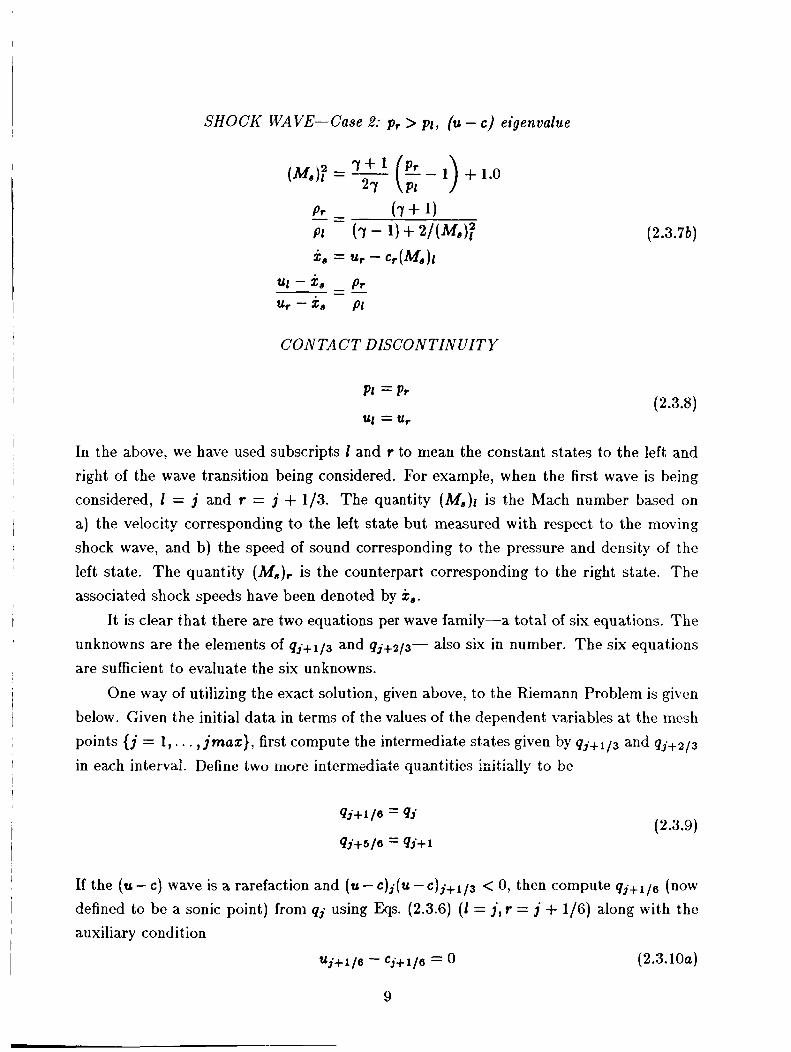
In the above, we have used subscripts 1 and t to mean the constant states to the left and right of the wave transition being considered. For example, when the first wave is being considered, 1 = j and t = j + 1/3 . The quantity (M,)I is the Mach number based on a) the velocity corresponding to the left state but measured with respect to the moving shock wave, and b) the speed of sound corresponding to the pressure and density of the left state. The quantity is the counterpart corresponding to the right state. The associated shock speeds have been denoted by x,.

It is clear that there are two equations per wave family-a total of six equations. The unknowns are the elements of qj+1/3 and q,+2/3- also six in number. The six equations are sufficient to evaluate the six unknowns.

One way of utilizing the exact solution, given above, to the Riemann Problem is given below. Given the initial data in terms of the values of the dependent variables at the mesh points { j = 1,. . . , j m a x } , first compute the intermediate states given by qj+1/3 and qj+2/3

in each intervai. Define two more intermediate quantities initially tc be

(2.3.9)

If the (u - c) wave is a rarefaction and (u - c ) j ( U - c)j+1/3 < 0, then compute qj+1/6 (now defined to be a sonic point) from qj using Eqs. (2.3.6) ( I = j , t = j + 1/6) along with the auxiliary condition

u j + l / 6 - cj+l /6 = (2.3.1 Oa)

9

Similarly, if the (u + c) wave is a rarefaction and the eigenvalue changes sign between j + 2/3 and J’ + 1, compute the sonic state qj+5/6 using Eqs. (2.3.6) ( I = j + 5/6, r = j + 1)

along with the auxiliary sonic condition

Then, define the various positive and negative flux differences of Eq. (2.3.4) by

(2.3.11)

Another approach to utilizing the Godunov scheme can be found in Ref. 24.

2.3.2 Osher’s Scheme

In Godunov’s scheme, when any of the waves is a shock, the equations for the intermediate states are not explicitly solvable for the unknowns and iterative techniques must be employed. In contrast, Osher’s numerical algorithm uses an approximate solution to the Riemann problem which results in explicit expressions for the intermediate state variables. Osher replaces the shock wave by overturned rarefactions”. Thus the wave transition for both nonlinear fields (for the (u - c) field and the (u + c) field) are described in terms of Eqs. (2.3.6) for rarefaction. The resulting six equations lead to explicit formulae for pj+1/3, tlj+1/3,pj+1/3, pj+2/3, ~ j + 2 / 3 , pj+2/3. Once the intermediate variables are computed, the corresponding fluxes are computed and included in the expressions for dfif using the same expressions presented earlier for Godunov’s scheme.

10

1

i I

I

I I

I

I

I

I

I

I I

I I

I

~

I

i t

I

I

I

I i I

I I

I

2.3.3 Roe's Scheme

Roe's algorithm is based on an approximate Riemann Problem2'. In Roe's approach, specially averaged cell interface values (denoted by subscript j + 1/2) are determined for density, velocity and enthalpy ( h = 7 p / ( ( 7 - 1)p) + (u2)/2)

from which the speed of sound c can be calculated as

(2.3.12)

Using these specially averaged values, Roe evaluates the Jacobian matrix and then consid- ers the approximate, linear, Riemann Problem given by

at each cell interface. The exact solution to this problem is given for the intermediate states as

(2.3.14)

(2.3.15)

with the parameters ai evaluated from the expressions

In the above equations, 1' are the left eigenvectors of the Jacobian matrix, evaluated such that they are orthonormal to the collection of right eigenvectors ri. The physical meaning of the parameters ai can be identified by considering the state space of dependent variables. In such a space, the equations for dq' (Eq. (2.3.15)) imply that the change dq' in dependent variables across each wave family is tangential to the corresponding right eigenvector and that ai is a measure of the magnitude of that change.

11

Once again, knowing ~ j + 1 / 3 , ~ j + 2 / 3 , etc., the various fluxes can be evaluated and included in the positive and negative flux differences in the following way which differs from the expressions in Eqs. (2.3.11) for Godunov's and Osher's scheme only because the Riemann Problem in Roe's scheme is linear, and consequently all the wave transitions are linear jump discontinuities. Thus, the various positive and negative flux differences of Eq. (2.3.4) are now defined by

~

1

For Roe's scheme, the values of df'* can also be directly defined to be

(2.3.17)

(2.3.18)

2.3.4 Split-Flux Scheme

The Split-Flux method developed by Steger and Warming22 is not directly connected to any Riemann Problem. But, it can be incorporated into the same algebraic framework by defining

dfj+'l/2 = [(A'*? q)r']j+l - [ (A if 1 i q)r']j , i = I , . . . , m . (2.3.19)

where Ai* = ( A i f I X 7 ) / 2 (2.3.20)

The Split-Flux scheme given above exploits the homogeneity property f = Aq of the Euler equations and is not applicable, in the form presented, to hyperbolic systems which do not have homogeneous fluxes.

2.3.5 Second-Order Accuracy

All the previous cases reduce to the same method for a system of linear equations. We have now seen the operational unification of several schemes in their basic, first-order

12

spatially accurate, form. A second-order accurate, fully upwind, semi-discrete formulation of all the previous four schemes is obtained by defining a second-order accurate numerical flux:

m

(2.3.2 1) fi+1/2 = h(qj+lrqj) + 5 ~ d f j ’ 1 / 2 - cdfi;3/2) - However, this construction is not Total Variation Diminishing (TVD) for systems of linear equations. The second-order accurate numerical flux has been presented as the combination of the first-order flux and some correction terms. A “TVD” scheme can be constructed by simply redefining the correction terms. Thus, the redefined numerical flux for a “TVD” scheme can be written as

( m i= 1 i= 1

h

In this redefinition, a flux difference is compared with the corresponding values in a neighboring interval and redefined by “flux-limiting” if necessary. The redefinition is according to the formulae:

where

and

where

“ 1 D - i+ N dfj-,/, = df;f,/, max b ) , min(b-, 1 ) (2 .3 .23~)

(2.3.233)

In the above, the function max [O,min(. - , b ) , min(b a compression parameter chosen in the interval

- , l)] is the flux limiter in which b is

1 5 b 5 2 (2.3.24)

The notation < z , y > denotes the inner product of vectors z and y. The rn-vector dg is a vector chosen to normalize the flux difference vector df, and its definition depends on

the particular upwind scheme under consideration. Two choices are given for dgi in the numerator. The first choice is preferred for theoretical reasons while the second choice (to the right of “or”) can lead to computational simplifications (as we shall see later for algorithms based on Roe’s flux decomposition).

An alternate set of definitions are possible for the flux-limited values of df* by making use of a symmetry property” of the particular flux limiter used in h s . (2 .3.23) . Expressing the ratio N/D as R, and the flux limiter as @(R), it can be shown that

@ ( R ) / R = @ ( l / R ) . (2.3.25)

where i+

dgj- 1 /2 > or N =< df!+ i+ 3 - 1 12’ dgj+ 1 /2

i+ (2.3.26b) =< dfj ,+, / , , dg j+ l /2 >

where

(2.3.26d)

Both definitions (Eqs. (2.3.23) and Eqs. (2 .3.26)) lead to identical schemes for scalar equations and systems of linear equations.

For Godunov’s, Osher’s and the Split-Flux schemes, a good choice for dg is based on the difference of the gradient of an entropy function. The entropy function is given by

The gradient of the entropy function (with respect to the dependent variables) is given by

g = v,v

14

(2.3.28)

The definitions for the various entropy gradient differences are simply obtained from those for the various flux differences given in Eqs. (2.3.11) by replacing f with g.

For Roe’s method, the normalizing vectors are directly defined as

dgif = Ii (2.3.29)

2.3.6 Summary

We have thus shown in this section how to operationally unify various first-order accurate upwind schemes and second-order “TVD” schemes. We have enclosed the term TVD in quotes here to denote the fact that the algorithms presented can be rigorously proved to be TVD when applied to scalar equations or systems of linear equations in one space dimension which also have TVD exact solutions. In fact, there are nontrivial theoretical difficulties in obtaining rigorously two-dimensional TVD schemes of high order ac~uracy’~ .

The one-dimensional Euler equations have been used in this section for illustrating the ideas. The algorithms presented here can easily be extended to two and three dimensions, and to arbitrary curvilinear coordinate systems. Such applications of the second order TVD scheme based on Osher’s Riemann Problem solver were presented for two dimensions in Ref. 2. A TVD formulation based on Roe’s approximate Riemann solver was extended to two-dimensional body-fitted coordinate systems in Ref. 5. In the latter, the spatial differencing was also coupled to the implicit relaxation methods to be described in Subsection 2.8. In the former reference, a two-step, explicit time-differencing algorithm was coupled to the TVD spatial discretization.

2.4 TVD SCHEME DESJGN BY PREPROCESSING

We now describe the preprocessing approach in terms of Roe’s approximate Riemann For Roe’s solver. Equivalent formulations can be constructed for the other methods.

scheme, we have already seen (Eq. (2.3.15)) that

m

i= 1

(2.4.1)

We now briefly review the postprocessing approach for constructing second-order accurate TVD schemes presented in Subsection 2.3.5. If we combine Eqs. (2.3.23) (taken with the

15

second option on dg) with Eq. (2.3.29) for Roe’s scheme, we would obtain the following definitions for the flux-limited values of the flux differences:

I I

(2.4.2a)

(2.4.2b)

On the other hand, starting with Eqs. (2.3.26) (with the second option for dg) , we can obtain

In the above equations (Eqs. (2.4.2) and Eqs. (2.4.3)),

where, in turn, ai& = ~ i & ~ i

(2.4.3a)

(2.4.3 b)

( 2 . 4 . 4 ~ )

(2.4.4b)

(2.4.5)

and “cmplim” is the compressive flux-limiter defined by

cmplim[z, y] =

sign(z) * max[0, min{ IzI, b y sign(z)}, min{b IzI, y sign(%)}] (2.4.6) .

The “compression” parameter has been denoted by 6 as usual. The above flux limiter is another form of the limiters used in Eqs. (2.3.23a,c). It was first suggested by Roe to Sweby” with b = 2, as a highly compressive flux limiter. Sweby presented its general form (1 5 b 5 2) and also compared it with other flux limiters.

In the preprocessing approach, by contrast, the slope-limited values of the dependent variables are first obtained. For example, to construct a second-order accurate scheme, we use piecewise linear distributions of the state change parameters ai to define

( 2 . 4 . 7 ~ )

16

at x = x- j+1/2 (limit from the left at the cell interface at ~ j + ~ / ~ ) , and

(2.4.7b)

a t x = x T+l/2 (limit from the right at the cell interface at ~ j+1 /2 ) . In the above, the “minmod” limiter is defined by

minmod [x, y] = sign(z) * max[O, min((x1, ysign(x)}] . (2.4.8)

Other limiters such as the one in Eq. (2.4.6) may be used. The formulae given here for the preprocessing approach are analogous to Eqs. (2.4.3) for the postprocessing approach.

Finally, we define the “TVD” numerical method in terms of the usual semi-discrete conservation form given in Ea. (2.3.2) by defining the numerical flux to be

The semi-discrete version of the scheme shown above was shown to converge for scalar convex conservation laws by Osher in Ref. 16.

2.5 APPLICATION TO GENERAL CONTROL VOLUMES

Both the preprocessing and postprocessing approaches can be extended to be applicable to general control volumes. In this subsection, we describe the extension of the preprocessing approach to two-dimensional, triangular control volumes (areas). Fig. 2.2 portrays one such cell ABC.

We begin with the two-dimensional conservation law

qt + v * F = 0 (2.5.1)

where V = Pa, + ja, is the gradient operator, and F is the vector flux. The integral formulation of the above conservation law, taken over the triangle ABC, is given by

(2.5.2)

17

D - C C

/I /

\ \ \ \ \ \ \ \ /

J

E

/ /

/ /

/ /

Fig. 2.2 Triangular control areas

18

where ds denotes a length increment along each side. The semi-discrete version of this integral conservation law can be written as

(2.5.3)

in terms of the representative numerical fluxes for each side.

define the numerical flux to be We now consider side BC in detail. The other sides are treated similarly. We first

In the above equation, - nBc = B C f i ~ c (2.5.5)

where f i ~ c is the unit outward pointing normal to side BC (outward implying outside the cell for which the vector from B to C is counterclockwise along the cell boundary), and BC is the length (positive) of side BC. The superscript in implies inside the triangle ABC and out denotes the outside of ABC. In our notation, in and out should be considered in conjunction with the subscript that denotes the side of the cell under consideration. In is inside the triangle for which the letter subscripts denoting the given side define a counterclockwise direction vector when the vector points from the first letter to the second letter. Out is outside that triangle or cell. The flux differences df* are computed with &?c as the left state and igu; as the right state, using one of the schemes described in Subsection 2.3. The flux differences are defined in terms of differences in the flux value denoted by lowercase f which is defined to be

-

The notation @2c and G% have been used to denote the values of q computed at side BC just to the inside and outside, respectively, using piecewise linear distributions for the state change parameters for each wave family. Thus,

(2.5.7)

We now have to define Qg% and pzc. We start with the latter, and we use Roe's Riemann Problem Solver for illustration.

19

Consider the inner triangle ABC and each side of it in turn. Each side separates two cells. Compute Roe’s average values for the elements of q (we can denote these by qau)

at each cell interface, and the corresponding orthonormal set of right and left eigenvectors ri(qau) and I i (qau) . Then, compute

I

I

(2.5.8)

Note that qout corresponding to each side denotes a different quantity depending on the outside triangle contiguous to the side under consideration. Next, define

m

i= 1

from which we can define

(2.5.9)

(2.5.10)

In the above equation, qABC is the average value of q ascribed to triangle ABC or its centroid, and sgc is the perpendicular distance from the centroid of the inside triangle ABC to side BC.

Using the above definitions, &% is simply computed as

(2.5.11) -out - -in qBC - qCB

where g2B is computed by considering cell CBD just like we considered cell ABC for computing ?&.

It must be remembered that other suitable limiters may be used instead of “minmod”. Also, preprocessing schemes based on any one of the basic schemes considered in Subsection 2.3 can be constructed for triangular control volumes. Roe’s method has been selected only for illustrative purposes. It is also clear that the procedure given in this subsection for triangular cells is equally and easily applicable to arbitrarily shaped control volumes as long as they are convex (the centroid should lie inside the cell). Finally, we point out that this procedure is tailored to extend the one-dimensional monotonicity preserving, piecewise linear extrapolation of piecewise constant data, to arbitrary shapes in higher dimensions. In fact, when applied to scalar one-dimensional problems, this is a TVD and convergent procedurelB.

20

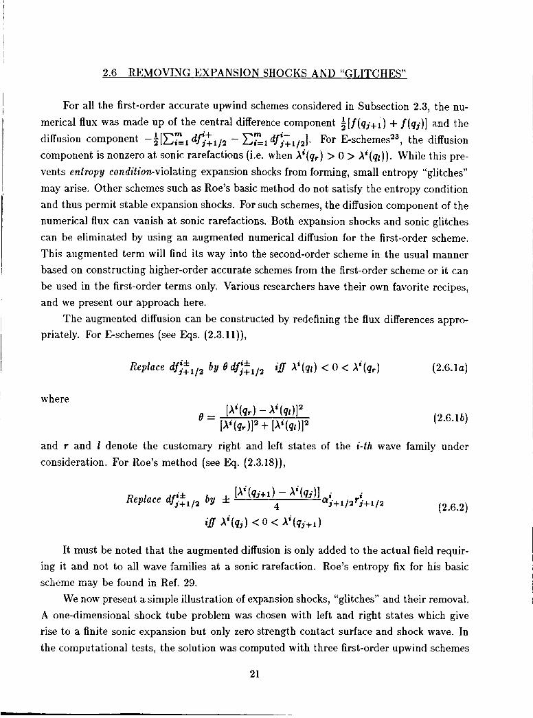
2.6 REMOVING EXPANSION SHOCKS AND “GLITCHES”

For all the first-order accurate upwind schemes considered in Subsection 2.3, the numerical flux was made up of the central difference component i[f(qj+l) + f(qj)] and the diffusion component -f[cLl df;.i,/, - E:, df;<112]. For E - s ~ h e m e s ~ ~ , the diffusion component is nonzero at sonic rarefactions (Le. when A i ( q r ) > 0 > A i ( q I ) ) . While this pre- vents entropy condition-violating expansion shocks from forming, small entropy “glitches” may arise. Other schemes such as Roe’s basic method do not satisfy the entropy condition and thus permit stable expansion shocks. For such schemes, the diffusion component of the numerical flux can vanish at sonic rarefactions. Both expansion shocks and sonic glitches can be eliminated by using an augmented numerical diffusion for the first-order scheme. This augmented term will find its way into the second-order scheme in the usual manner based on constructing higher-order accurate schemes from the first-order scheme or it can be used in the first-order terms only. Various researchers have their own favorite recipes, and we present our approach here.

The augmented diffusion can be constructed by redefining the flux differences appropriately. For E-schemes (see Eqs. (2.3.11)),

where

(2.6.1 b )

and r and 1 denote the customary right and left states of the i-th wave family under consideration. For Roe’s method (see Eq. (2.3.18)),

(2.6.2)

It must be noted that the augmented diffusion is only added to the actual field requiring it and not to all wave families at a sonic rarefaction. Roe’s entropy fix for his basic scheme mzy be fmnd io Ref. 29.

We now present a simple illustration of expansion shocks, “glitches” and their removal. A one-dimensional shock tube problem w a s chosen with left and right states which give rise to a finite sonic expansion but only zero strength contact surface and shock wave. In the computational tests, the solution was computed with three first-order upwind schemes

21

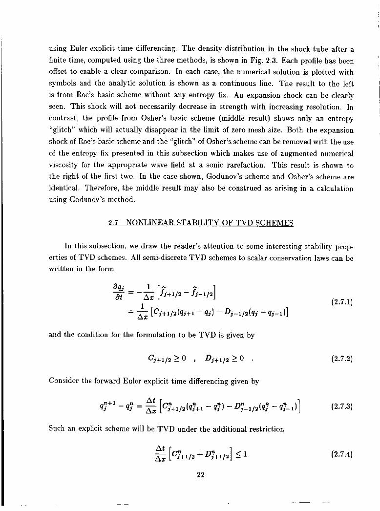
using Euler explicit time differencing. The density distribution in the shock tube after a finite time, computed using the three methods, is shown in Fig. 2.3. Each profile has been offset to enable a clear comparison. In each case, the numerical solution is plotted with symbols and the analytic solution is shown as a continuous line. The result to the left is from Roe’s basic scheme without any entropy fix. An expansion shock can be clearly seen. This shock will not necessarily decrease in strength with increasing resolution. In contrast, the profile from Osher’s basic scheme (middle result) shows only an entropy “glitch” which will actually disappear in the limit of zero mesh size. Both the expansion shock of Roe’s basic scheme and the “glitch” of Osher’s scheme can be removed with the use of the entropy fix presented in this subsection which makes use of augmented numerical viscosity for the appropriate wave field at a sonic rarefaction. This result is shown to the right of the first two. In the case shown, Godunov’s scheme and Osher’s scheme are identical. Therefore] the middle result may also be construed as arising in a calculation using Godunov’s method.

I

I

I I

2.7 NONLINEAR STABILITY OF TVD SCHEMES

In this subsection, we draw the reader’s attention to some interesting stability properties of TVD schemes. All semi-discrete TVD schemes to scalar conservation laws can be written in the form

I (2.7.1)

and the condition for the formulation to be TVD is given by

C j + 1 / 2 2 0 t o j + 1 / 2 > O

Consider the forward Euler explicit time differencing given by

At n q j ) - 0 , 3 - 1 / 2 ( ~ i n - q;-1)]

Such an explicit scheme will be TVD under the additional restriction

At - Az [‘;+I/, + Dj”+1/2] 5

22

(2.7.2)

(2.7.3)

(2.7.4)

* v) 2 w

t

n

RIEMANN PROBLEM SOLUTION DENSITY PROFILE

SCHEME

X

Fig. 2.3 Expansion shocks, “glitches”, and entropy fix

23

This mathematical framework of fully discrete, explicit TVD schemes was first introduced by HartenQ. I

Corresponding to every TVD scheme, one can define the underlying non-TVD algo- I

rithm. In fact, all semi-discrete TVD schemes can be obtained by starting from a higher order conventional upwind scheme and applying flux limiters to the appropriate flux differences. Conversely, given a TVD scheme with flux limiters, the corresponding non-TVD scheme can be obtained by simply redefining the flux limiter @(R) (see J3q. (2.3.25)) to be ~

@ ( R ) = R , (2.7.5)

which amounts to removing the limiting from the limiter. The underlying non-TVD schemes corresponding to all the higher order semi-discrete

TVD schemes considered so far and those that will be presented in Subsection 2.9 are linearly unstable (unconditionally) when used with Euler explicit time differencing. All the TVD schemes, much to the contrary, are nonlinearly stable, under the restrictions imposed by Eqs. (2.7.2,2.7.4). Here, we use the term “nonlinear” to signify the fact the TVD scheme is a nonlinear finite difference scheme, by virtue of the nonlinear flux limiters, even when applied to linear equations. This nonlinear stability can be exploited in many ways. For example, newly derived semi-discrete algorithms can be numerically verified very easily by coupling the TVD space differencing with Euler explicit time differencing. Similarly, complex computer programs using implicit time differencing, etc., can be de- bugged more easily by checking them out in Euler explicit mode. It must also be pointed out however, that TVD schemes using Euler explicit time differencing usually have time step (Courant number) restrictions which are fractions of unity. Thus, they may not be efficient algorithms to reach time-asymptotic steady states.

2.8 DIAGONAL DOMINANCE IN TVD FORMULATIONS

In this subsection, we review how the TVD property can lead to diagonally dominant implicit schemes. Consider the Euler implicit time differencing coupled to the semi-discrete form given in Eq. (2.7.1):

Grouping all the unknowns at the new time level, we get

24

(2.8.2)

It is obvious that, if the space differencing is semi-discrete TVD, then I

Cn+' ' 0 9 Dn+l j+1/2 > o - , j+1/2 - I

I I

and that the left-hand side of h. (2.8.2) is diagonally dominant by rows. Now consider the two-dimensional scalar conservation law given by

(2.8.3)

, qt + fi + 9y = 0 (2.8.4)

Let us discretize fx and gI independently with uni-dimensional TVD approximations and construct the implicit algorithm given by

I At

I Since I

I

(2.8.5)

(2.8.6)

I this multi-dimensional implicit scheme is also diagonally dominant by rows. I The one-dimensional requirements for obtaining a one-dimensional TVD scheme are

not enough to construct a TVD scheme in two dimensions. Notwithstanding this observation, the positivity conditions on the coefficients C and D are enough to provide diagonal dominance for the multi-dimensional implicit scheme.

While the above paragraphs illustrate the connection between the TVD property and diagonal dominance, Eq. (2.8.1) and J3q. (2.8.5) are not directly useful as numerical algorithms because the positive coefficients C and D are nonlinear functions of qj. Harteni3 introduced a family of unconditionally stable TVD schemes (for one-dimensional scalar equations or constant coefficient systems). The simplest of these was based on freezing C and D of Eq. (2.8.1) at time level n instead of defining them at n + 1:

(2.8.7)

However, while steady-state solutions satisfying EQ. (2.8.7) satisfy the discrete analog of the conservation principle, transient solutions do not. Two-dimensional applications (using

25

the alternating-direction implicit method) of such an algorithm to the Euler equations are shown in Ref. 26. These approaches do not utilize the diagonal dominance property to any numerical advantage.

In Ref. 5, on the other hand, various ways of constructing relaxation methods for unfactored implicit schemes are presented, all of which exploit the diagonal dominance property. One possible approach is outlined here for illustration.

The nonlinear discretization given in l3q. (2.8.5) is a consistent, conservative approximation to Eq. (2.8.4). We can devise many relaxation methods to solve the equation. For notational and conceptual simplification, we first consider the unknowns q:+' as new variables Qj. Then, for each grid point j, one can construct the nonlinear equation

(2.8.8)

Taken over all the grid points, this results in a nonlinear system of equations of the type

WQ) = 0 (2.8.9)

which we can consider solving by the Newton procedure

where superscript t! is an iteration index. Instead of the full Newton linearization, we can try a "TVD" linearization implied by

(2.8.1 1)

26

In the above equation, obvious subscripts have been left out, and

It can be seen that Eq. (2.8.11) is a diagonally dominant (by rows) equation for QL+I. Consequently, instead of using this “Quasi-Newton’) method, we can obtain iterative convergence to zero of the right-hand side of &. (2.8.11) by using relaxation methods. Various relaxation methods can be constructed by neglecting various terms from the left-hand side operator, but by always retaining the diagonal operator in its entirety. At convergence, QL+’ - QL = 0 , and Eq. (2.8.2) would be satisfied to the desired degree (depending on the convergence tolerance). After updating the dependent variables to the next time level, the relaxation iterations can be repeated for the next time step.

The reader is referred Section 3 for a more detailed presentation of the material given here. Many classes of relaxation schemes such as pointwise, linewise, Gauss-Seidel, and non-Gauss-Seidel methods are considered therein along with a discussion of the advantages of relaxation methods vis-a-vis methods which use approximate factorization. The theory has been developed here (in Sections 2 and 3) only for scalar equations. While the construction of relaxation methods for systems of equations is straightforward and many examples are given in Section 3 for the Euler equations, more study is required to establish ’il firmer theoretical foundation for this case.

2.9 REMARKS

Many topics related to the computational aspects of modern TVD schemes have been presented in this section. The operational unification of upwind schemes is designed to make the reader aware of the underlying, but not always obvious, similarity between seem- ingly disparate approaches. Thus, methods based on Godunov’s, Roe’s, Osher’s, or the Split-Flux scheme of Steger and Warming, can all be put into the same framework. Second- order accurate TVD schemes based on any of the above can be constructed using either the postprocessing or preprocessing approaches. Both approaches can be extended to general control volumes (triangles in two-dimensions, for example). The preprocessing algorithm for triangles has been presented in this report. Each of the basic underlying first-order schemes can result in either expansion shocks or “glitches”, and methods for their elimination have also been studied here. The nonlinear stability of single-stage explicit higher-order TVD schemes has been pointed out. The link between TVD schemes and diagonal dominance has been brought out along with a discussion of relaxation algorithms which are therefore made possible. Finally, a new family of low truncation error

27

(or high accuracy) TVD schemes have been presented for scalar equations using the postprocessing approach. While much of the material presented here is new, an attempt has

comprehensive picture of various aspects of the subject. also been made to fill in the gaps left by previous technical manuscripts, and to provide a I

It is obvious that the new framework being developed is very flexible and large. It will be some time yet before most of the options are explored and compared with each other. Is the preprocessing approach better than the postprocessing method? How useful are algorithms constructed for triangular control volumes? How much better are the relaxation methods when compared to approximate factorization methods? These are but a minor fraction of the questions which must be answered. It is also obvious, however, that high resolution TVD schemes have come of age. They herald a new era of Computational Fluid Dynamics, an advancement in the state of the art, at least a small replacement of some of the art with science, and the addition of a little more mathematical rigor into the engineer’s craft.

I

~

Section 3.0 RELAXATION METHODS FOR

UNFACTORED IMPLICIT UPWIND SCHEMES

3.1 SUMMARY

The last part of the previous section developed the concept of diagonal dominance inherent in TVD formulations. In this section, this property is used to construct relaxation methods for unfactored implicit upwind schemes for hyperbolic equations. The theoretical basis is explained further using linear and nonlinear scalar equations; construction of the method for the unsteady Euler equations (nonlinear system) is but a natural extension. One of the important advantages of the above methods vis a vis factored implicit schemes is the possibility of faster convergence to steady state, as illustrated by the results. Several classes of relaxation schemes such as pointwise, linewise, Gauss-Seidel, and non-Gauss- Seidel methods are discussed, along with various strategies for convergence.

3.2 INTRODUCTION

Implicit finite difference schemes for hyperbolic systems, including the unsteady Euler equations, have for the most part used central space differencing and have relied upon the techniques of approximate factorization or fractional steps to handle multi-dimensions [Refs. 31,321. Even researchers using various upwind schemes (the split-flux method or Harten’s scheme) [Refs. 33,261, have resorted only to these conventional approximate ways of splitting the multi-dimensional operators into one-dimensional operators (which are then solved efficiently using block-tridiagonal elimination). A plus-minus splitting scheme [Ref. 221 has also been attempted for the split-flux scheme leading to a different but once again approximately factored implicit scheme. In contrast to the above, relaxation methods are propxed hcre for mfactored forms of implicit upwind schemes. The new algorithms owe their existence to the beneficial properties of modern upwind schemes. The unfactored algorithms can make dramatically increased speeds of convergence possible when only a time-asymptotic steady-state solution is desired but can also be used as efficiently as the factored schemes for computing t rdy unsteady flows.

The purpose of this section is threefold: a) to show what the relaxation algorithms are, b) to bring out the theoretical justifications, and c) to illustrate their efficiency. We begin with a discussion of unfactored implicit schemes for the linear scalar equation in two spatial dimensions based on first-order accurate upwind differencing. The theory is then

29

Results for four examples are presented along with convergence histories and computational times.

3.3 LINEAR SCALAR EQUATIONS

ut + au, + buy = 0. (3.3.1)

We begin by assuming a and b to be positive. A simple implicit upwind scheme may be written as

(3.3.2)

The subscripts j and k indicate the spatial coordinates x and y. The scheme is first-order accurate in space and time. The time-step index has been denoted by the superscript n.

3.3.1 Diagonal Dominance

Regrouping terms in Eq. (3.3.2), we obtain

(3.3.3)

It is clear that if this is cast in matrix notation and boundary values of u:,:' and u;:' are known, the system is diagonally dominant by rows and columns. In other words, if the elements of the matrix are dj,k,

(3.3.4a)

and

30

(3.3.4 b)

The surplus in the diagonal term is due to the term l /(At). It is also obvious for the case under discussion (a > 0, b > 0) that in the matrix notation

A (u"" - u") = b, (3.3.5)

A is lower triangular and is easily and efficiently inverted. This last observation is true when l/(ht) -+ 0 also. 3.3.2 Convergence of Approximately Factored Methods

For unfactored methods for linear equations, proper choice of boundary conditions, and assuming At -+ 00 or l /(At) -+ 0, one time step is all that is required to reach steady state. However, this is not true for factored implicit schemes of the type

(3.3.6) (un+l - u") = - (a-& At + b%,) u".

A% AY

In the above equation, 6, and 6, are finite-difference operators. Writing Q. (3.3.6) or Eq. (3.3.2) as

Un+l - - LU", (3.3.7)

the time-asymptotic steady state denoted by urn must satisfy

uw = Lurn, (3.3.8)

and the difference between un and urn must satisfy

It can be shown using a von Neumann analysis that

Limit At -+ 00 (7 (LEq. (3.3.2)) = 0,

Limit At -+ 00

(LEq. (3.3.8)) = 1,

(3.3. IOU)

(3.3.10b)

31

Numerically, for the two-dimensional scalar wave equation under consideration, for uniform grid and wave speeds, the optimum time step for convergence for the factored scheme is not far from that implied by

At At Ax Ay

a- = b- - - 1,

ie., not much above a C-F-L number of unity. It is thus obvious that there may be penalties associated with factored implicit schemes that are not commonly thought of - and it may be very much to our advantage to construct unfactored implicit schemes. The diagonal dominance property discussed before will enable us to construct relaxation methods for unfactored implicit upwind schemes.

3.3.3 Diagonal Dominance for Arbitrary Coefficients

When coefficients a and b are of the type

and thus of possibly arbitrary signs (not just only positive or only negative), an implicit upwind scheme can be constructed as an equation that automatically switches from backward to forward differencing depending on the signs of a and b.

Once again, regrouping terms, we obtain

32

(3.3.12)

(3.3.13)

and thus find diagona dominance.

diagonal dominance. First-order spatially accurate upwind schemes have a way of naturally giving rise to

3.4 NONLINEAR SCALAR EQUATIONS

We have thus far considered a linear equation and first-order accurate spatial differencing. We now examine nonlinearity and second-order accuracy. A central theme throughout this section will be the concept of a Total Variation Diminishing (TVD) scheme. It will be shown that it is this TVD property (applied to individual spatial dimensions) that results in diagonal dominance even for second-order accurate schemes for both linear and nonlinear equations. Simple approaches to second-order accuracy such as using

1.5uj - 2 ~ j - 1 + 0.5uj-2 AZ

212 - will not in general lead to successful relaxation methodologies.

We now consider the nonlinear equation

(3.4.1)

ut + fz + gu = 0. (3.4.2)

The corresponding fully nonlinear implicit version of an upwind scheme may be written as

(3.4.3)

Once again, 6, and 6, are suitable upwind discretization operators (either first-order or second-order accurate).

3.4.1 Diagonal Dominance and the TVD Property

All conservative flux derivative terms for the scalar conservation law (E&. (3.4.2)) may be rewritten using the notation [Ref. 91

33

The fully nonlinear implicit scheme (Q. (3.4.3)) may then be rewritten as

It is then obvious that the condition for row diagonal dominance will be

(3.4.4) I I

(3.4.5) I

(3.4.6)

For those readers familiar with TVD schemes [Ref. 91, the similarity between the conditions of Eq. (3.4.6) and the conditions for obtaining a one-dimensional TVD explicit scheme will suggest itself. An explicit scheme similar to Eq. (3.4.5) can be arrived at by substituting n for n + 1 in all the spatial difference terms of Eq. (3.4.5). The corresponding conditions for obtaining the TVD property for the one-dimensional restriction would be given by relations similar to Q. (3.4.6) with the superscript n substituted for n + 1. In fact, the general necessary condition for a time-continuous met hod

(3.4.7)

to be TVD is given by Eq. (3.4.6) with the superscripts n + 1 deleted altogether

The one-dimensional requirements for obtaining a one-dimensional TVD scheme are not enough to construct a two-dimensional TVD scheme (if required). In other words, if we construct a two-dimensional algorithm based on the coefficients C2, CY and D5, DY,

34

even though the x-coefficients and the y-coefficients are independently capable of giving rise to one-dimensional (in x or y) TVD schemes if they satisfy the positivity constraints, together they may not result in a two-dimensional TVD scheme. Notwithstanding this observation, the positivity conditions are enough to provide diagonal dominance for the relaxation iterations to be used in the unfactored implicit scheme.

The TVD constraints are compatible with second-order accurate schemes [Refs. 9,10,2] and have been the basis for the construction of high resolution explicit upwind schemes in the past along with factored implicit schemes. For linear systems and nonlinear scalar equations in one spatial dimension, the TVD property guarantees t,hat when the exact solution is monotonicity preserving, the numerical solution too behaves thus. This en- ables oscillation-free solutions. It must also be pointed out here that proofs of the TVD properties of upwind algorithms are lacking for nonlinear systems of equations. However, multifarious applications consistently show oscillation-free properties in one-dimensional problems. For multidimensional problems, in general, the exact solution may not be monotonicity preserving. However, when schemes that are one-dimensionally TVD are applied in naturally extended constructions [Ref. 21 to two-dimensional problems, equally pleasing (essentially oscillation-free) results are obtained.

3.5 RELAXATION METHODS

We have thus far pointed out how to achieve diagonal dominance for scalar equations (both linear and nonlinear and for both first-order and second-order accuracy). We now provide the infrastructure for the construction of relaxation methods. This framework will be able to unify various relaxation methods and convergence strategies, and will be developed directly for systems of hyperbolic conservation laws in a natural extension of what is possible for single equations. The non-conservation law form of the governing equations can also be considered as a simple modification of the methods developed here (the non-conservation law form for scalar equations has already been considered in Section 3.3).

We consider as a prototype equation-set, the unsteady Euler equations in Cartesian coordinates:

Q ~ + & + F , = o . (3.5.1)

Arbitrary geometries follow easily and will not be covered here. We shall march these equations in time until a time-asymptotic steady state is reached (when this is of interest, of course).

We first write the nonlinear implicit scheme

35

Q"+ 1 - Qn + 6,26+' + bUF"+' = 0.

At (3.5.2)

The difference operators 6, and 6U are assumed to be based on suitable upwind schemes of desired accuracy. By virtue of its nonlinearity, the above EQ. (3.5.2) is not directly solvable for the dependent variables Qn+'. Our approach is to construct a sequence of approximations denoted by q' such that

q' + Q"+'. Limit i > > l

(3.5.3) I I

I The superscript i here is a subiteration index between two time levels.

A Newton method can be constructed for q'+' by linearizing Eq. (3.5.2) about the known subiteration state denoted by superscript i as follows:

For the Newton method, we have to use on the left hand side (LHS) the true Jacobians of the terms on the right hand side (RHS) and this is indicated above. The numerical solution of the full Newton method in two or more dimensions is too time consuming. On the other hand, various relaxation methods are easily obtained from Eq. (3.5.4) by retaining various terms on the LHS and discarding the others. All terms contributing to the diagonal are always retained. Other variations result by not using the true Jacobian matrices, etc. Many of these possibilities are discussed in the following subsections under the titles of linearization strategies and various relaxation strategies.

3.5.1 Linearization Strategies

We have discussed the Newton linearization using the true Jacobians. We now cover other options.

3.S.1.1 Conservative Linearization

The Newton linearization results in a scheme that is conservative in space and time (assuming that the spatial differencing is conservative). This property is true even if the subiterations (indicated by the superscript i ) between two time levels do not fully converge.

36

However, diagonal dominance may not exist during the subiterations for all choices of time step size. However, since the fully nonlinear scheme is diagonally dominant by virtue of the unidimensional TVD property of the spatial discretization, it is expected that for “reasonable” (even if large) values of At, the diagonal dominance will be preserved. The subiterations can proceed with various relaxation methods valid for diagonally dominant systems.

We can preserve conservative linearization even if we depart from the true Jacobians of the RHS terms, as long as the LHS spatial difference terms are conservative operators on their own, ie., of the type

This can arise when the RHS corresponds to one upwind scheme and the LHS corresponds to another. Even here, the LHS need not be the true Jacobian of the second upwind scheme. The advantage of the Newton method is the possibility of quadratic convergence. Since by adopting relaxation methods, we depart from the true Newton method anyway, it may not be an additional heavy penalty to resort to a LHS which is not the true Jacobian of the RHS. Using pseudo-Jacobians comes in handy for upwind schemes for which it is cumbersome to obtain the true Jacobian matrices or when simplifications are made to save computational time.

3.5.1.2 Non-Conservative Linearization

We can even resort to non-conservative linearization strategies. Here, the LHS spatial difference operators are not representable in the discrete conservation law form of Eq. (3.5.5). If the subiterations converge, the overall time step is still conservative in space and time because the solution will satisfy the condition RHS = 0, and the RHS will be a fully conservative operator. However, for partially converged subiterations, time conservation will be lost. Time-asymptotic steady-state solutions will possess the required conservation properties.

One possible advantage in this approach is that diagonal dominance can be unconditionally preserved during the subiterations [Ref. 261. Such a scheme can be obtained by freezing the positive coefficients C and D of a TVD scheme, writing the linearized equations as

37

1 i

(C,”,!)SAj++ +-(DX Ax 3 - a A ) A,-A a

(q’f’ - q’) 1 i 1 - - A k + * G (D:-t>i AY

I

(3.5.6) At Ax

= - [” - Qn

3.5.1.3 Frozen Coefficients

Other variations are possible by freezing the various matrices and terms occurring in the RHS and LHS at various levels.

3.5.1.4 Spatial Accuracy of RHS and LHS

The above three variations can all be obtained when the RHS is chosen to correspond to a second-order spatially accurate upwind scheme and the LHS to a first-order accurate upwind scheme. The RHS can also be written as a combination of a first-order scheme and second-order correction terms [Ref. 21. These second-order correction terms can be lagged at the nth time level without causing instabilities (based on linear stability analysis). In a Gauss-Seidel approach (to be described later), where the RHS is computed using latest available values during every subiteration, these second-order correction terms can also be lagged at the ith subiteration level (without using latest available i + lSt level values). The LHS can either be conservative or non-conservative by choice (Sections 3.5.1.1 or 3.5.1.2).

3.5.2 Pointwise Relaxation Methods

We now assume that one of the above linearizations has been chosen. By discarding all terms from the LHS except those going into the diagonal block matrix at every point, we obtain the pointwise relaxation method.

3.5.3 Line Relaxation Methods

By retaining all terms in the diagonal and all terms in the larger matrix corresponding to all points on a chosen line, one obtains a line relaxation method. The line of points can be a constant 2 line, a constant y line, or a circular line (connecting all points closest to

38

all outer boundaries and similar concentric lines), etc. It can also be a zig-zag line (whose j , k subscript pairs can be given for example by 1 , 1 - 1,2 - 2,2 - 2,3 - 3,3 - . -, etc.).

3.5.4 Gauss- Seidel Met hods

The pointwise or linewise relaxation methods can further be subdivided into Gauss- Seidel (GS) and non-Gauss-Seidel (NGS) methods. In the GS methods, the RHS is evaluated using the latest available values of the dependent variables. The advantage of the GS method is the quick propagation of changes in the solution. For example, for the linear wave equation, when the coefficients a and b are positive, a pointwise GS method with the sweep directed from left to right and bottom to top is identical to a direct solution of the matrix system of equations. Thus, it will yield steady-state solutions in one forward sweep (one fell swoop) if l /(At) is set to zero. The main disadvantage of the GS methods is that they are not very suitable for vectorization.

3.5.5 Non-Gauss-Seidel Methods

In contrast to GS methods, the RHS in NGS methods are computed using previous level values even if current level ( i + 1) values are available for some points or lines. Thus, these methods are more suitable for vectorization. Also, the operation count for these NGS methods per cycle of subiterations can be lower than for a cycle of GS subiterations for a second-order accurate discretization of the RHS. On the other hand, numerical signal propagation in NGS methods can be slower than in GS methods.

One line-implicit but NGS method is appropriately called the Zebra scheme, and the corresponding pointwise NGS method is called the Checkerboard scheme. In the Zebra scheme, the grid points are divided into alternate black and white lines (like the stripes on a Zebra). In the first subiteration sweep, only the even numbered (or say the black) lines are updated, followed in the next sweep by an update of the odd numbered (or white) lines. In the Checkerboard approach, which is pointwise, the points are divided into black and white ones like the pattern in a checkerboard (in two dimensions, the blacks can be those points whose two spatial indices sum up to even number and the whites can be those whose indices sum up to odd value). The blacks and whites are updated in alternate sweeps. In either NGS method under discussion, the second sweep makes use of the values updated in the first sweep, and so on.

39

3.5.6 Pointwise Nonlinear Convergence ~ ,

1 In considering points by themselves, or as part of a line in the GS or NGS methods, we can also iterate on that point or line to nonlinear convergence before proceeding to the next point or line. The usual procedure is only to solve the linearized equations for a point or line and proceed to the next point or line.

3.5.7 Alternatinn Sweeps

For the GS methods, when both positive and negative signal propagations are present, it is best to alternate a forward sweep of points (lower left to upper right) with a backward sweep. In pointwise methods, this is not applicable. For fully supersonic flows, the backward sweep in the supersonic flow direction is unnecessary.

~ 3.5.8 Number of Subiterations

When only a time-asymptotic steady-state solution is of interest, it is not necessary to fully converge the subiterations between time steps.

3.5.9 Time-SteD Choice

For linear equations, all of the relaxation processes mentioned above are unconditionally stable and lead to faster convergence with larger time steps. For nonlinear equations, because of linearization errors and their effect on diagonal dominance, etc., the usual procedure is to couple the time-step to the residue (the magnitude of the deviation from steady state). We allow the time step to increase as the residue drops.

At those points in the flow-field where the eigenvalues of the coefficient matrices for the hyperbolic equations vanish, it will not be possible to take an infinitely large time step. This will be obvious if one looks at the linear equation (Eq. (3.3.1)) and the corresponding scheme given by Eq. (3.3.3) and set a, b, and l /(At) to zero.

Spatially varying time steps may also prove very useful to reach convergence faster. The drawback of this approach for some problems may be that the numerical transients do not have to bear any close resemblance to the real or physical transient associated with physically reasonable initial data and this may cause failure of the convergence process by giving rise to negative values for pressure, density, etc.

40

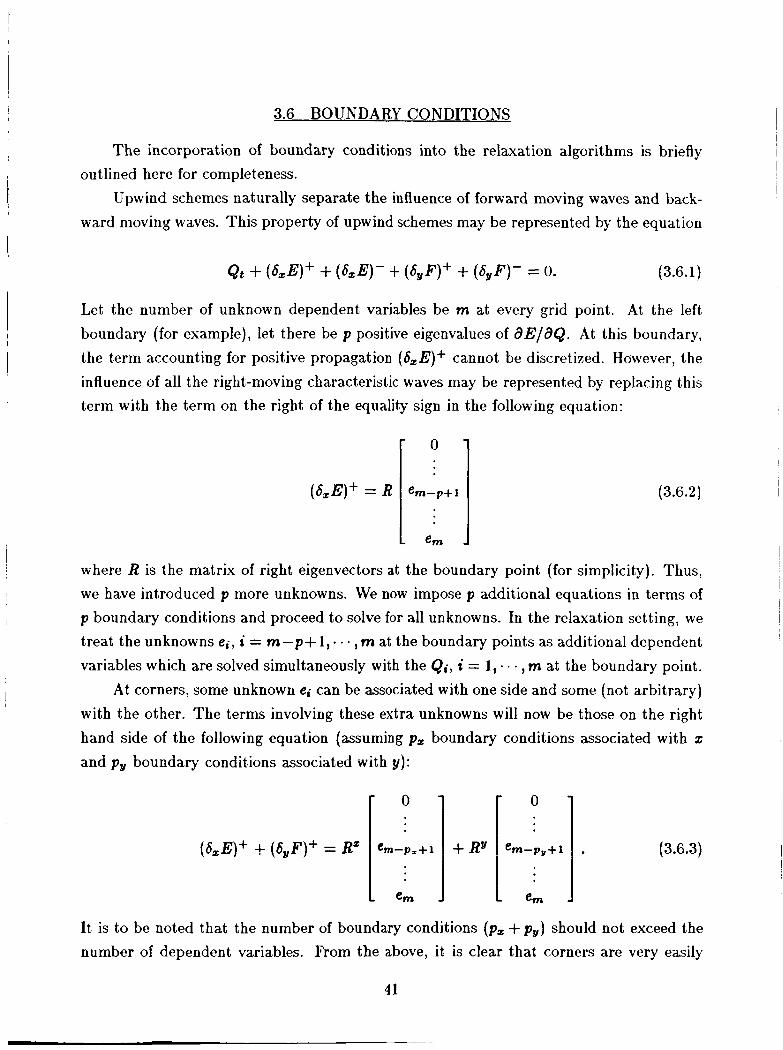
3.6 BOUNDARY CONDITIONS

The incorporation of boundary conditions into the relaxation algorithms is briefly

Upwind schemes naturally separate the influence of forward moving waves and backward moving waves. This property of upwind schemes may be represented by the equation

outlined here for completeness.

Qt + (&E)+ + (&E)- + (byF)+ + (6,F)- = 0. (3.6.1)

Let the number of unknown dependent variables be m at every grid point. At the left boundary (for example), let there be p positive eigenvalues of aE/aQ. At this boundary, the term accounting for positive propagation (&E)+ cannot be discretized. However, the influence of all the right-moving characteristic waves may be represented by replacing this term with the term on the right of the equality sign in the following equation:

(3.6.2)

where R is the matrix of right eigenvectors at the boundary point (for simplicity). Thus, we have introduced p more unknowns. We now impose p additional equations in terms of p boundary conditions and proceed to solve for all unknowns. In the relaxation setting, we treat the unknowns e;, i = m-p+ 1, - .. , m at the boundary points as additional dependent variables which are solved simultaneously with the Q;, a = 1, - , m at the boundary point.

At corners, some unknown e; can be associated with one side and some (not arbitrary) with the other. The terms involving these extra unknowns will now be those on the right hand side of the following equation (assuming ps boundary conditions associated with x

and py boundary conditions associated with y):

(3.6.3)

It is to be noted that the number of boundary conditions (pz + py) should not exceed the number of dependent variables. From the above, it is clear that corners are very easily

4 1

treated in this approach to boundary condition implementation. Various boundary conditions such as surface tangency, inflow, outflow, shock-fitting, etc., have all been successfully treated using the above approach.

3.7 RESULTS

Results are now presented for four examples:

Problem 1 - Critical flow past a circular cylinder ( M , = 0.40).

Problem 2 - Transonic flow past the circular cylinder ( M , = 0.45).

Problem 3 - Regular reflection of an oblique shock wave by a flat plate ( M , = 2.9, incident angle between shock wave and flat plate is 29 degrees).

Problem 4 - Symmetric transonic flow past a circular arc airfoil ( M , = 0.85, 10% thick).

The unsteady Euler equations were solved for all the problems. The first problem was solved using the spatial differencing associated with the Split Coefficient Matrix (SCM) method [Refs. 34,351. The last three problems were solved using a conservative upwind scheme based on the approximate Riemann solver developed by Roe [Refs. 20,361. The first problem used the pointwise GS method. The last three problems were solved using both the line GS method and the Zebra NGS method and these two methods are compared in what follows.

Fig. 3.1 shows the computational grid for problems 1 and 2. Fig. 3.2 displays Mach number contours for problem 1. The line of symmetry has been treated as an imperme- able boundary. Fig. 3.3 compares the pressure distributim on the surface of the cylinder obtained using the SCM method and a potential flow solver [Ref. 371. Fig. 3.4 portrays the time histories of the residue and time step for problem 1. It is obvious that a strategy of increasing the time step as the residue drops has been employed. Five orders of magnitude drop in residue takes but 25 time steps. Each time step comprises one forward and one backward sweep.

Fig. 3.5 depicts the Mach number contours for problem 2, in increments of 0.1. Fig. 3.6 presents the distribution of pressure coefficient Cp on the surface of the cylinder. Once again, the Euler solution is compared with the solution to the full potential equation [Ref. 371. Figs. 3.7 and 3.8 illustrate the computational grid and pressure contours for problem 3. Fig. 3.9 shows the pressure profiles along y = 0 and y = 0.5. Fig. 3.10 is part of the computational grid for problem 4. Figs. 3.11 and 3.12 portray Mach number contours and the surface Cp profile for problem 4. The results for problem 3 can easily

42

be compared with exact solutions. Results for problem 4 can be compared with those in Ref. 38, for instance.

We conclude this section with two tables. Table 3.1 compares the operation counts for a line GS method and a Zebra scheme. The second-order correction terms for the GS method were kept frozen at the ith subiteration level at every sweep. The references to Riemann Flux and Jacobian in Table 3.1 are based on the fact that flux-difference upwind schemes such as Roe’s or Osher’s [Ref. 21 are based on approximate Riemann solvers. All the numerical entries in the tabulation denote computations per point. It is obvious that the Zebra scheme requires about half the work of the GS scheme.

Table 3.2 shows the CPU times for problems 2, 3, and 4 on a VAX 11/780 minicom- puter. For problem 3, because the flow is entirely supersonic in the z direction, only a forward z sweep is used for the GS method. It is obvious that in general, the Zebra scheme, even without vectorization, is quite efficient for transonic problems. For supersonic problems, due to the nature of signal propagation, the GS method is more efficient.

3.8 REMARKS

A new set of implicit schemes has been presented for hyperbolic systems of equations. These algorithms do not resort to approximate factorization. They are based on various relaxation methods. The new algorithms can be as efficient as approximately factored algorithms for following the transients of an unsteady problem. For problems where only a time-asymptotic steady state is of interest, the new methods can lead to much more rapid convergence because very large time steps can be taken. Conventional approximately factored schemes will not be able to match this performance.

The new implicit scheme is developed only for and is based on the beneficial properties of upwind difference methods. While modern upwind schemes are very robust and highly reliable, a drawback is their computational cost because of increased number of arithmetic operations. The new implicit method presented here more than offsets this disadvantage. In fact, it should be possible to obtain better solutions faster and more reliably using the just described form of implicit upwind schemes.

43

COMPUTATIONAL GRID

Y

-1.5 -0.9 -0.3 0.3 0.9 1.5 X

Fig. 3.1 Computational grid for circular cylinder problem

44

3.0

2.4

1.8

Y

1.2

0.6

0

MACH NO. CONTOURS

M, = 0.4

-1.5 -0.9 -0.3 0.3 0.9 1.5

X

Fig. 3.2 Mach number contours for Moo = 0.4

45

i-251 PRESSURE PROFILES

M = 0.4 00

W pt

0.50 ! . I d

-90 -54 -1 0 10 54 90 THETA

Fig. 3.3 Surface pressure for M,, = 0.4

46

RESIDUE TIME HISTORY PLOT

0

-1

-2 w 3 n

a -3

w

-4

-5

-6

6 -

- 5

- 4

3 - c a 3

n

2

1

0

-

t DTAU

I 0 25 50 75

TIME STEPS

Fig. 3.4 Time histories of residue and time step

47

MACH NO. CONTOURS 3.0-

2.4-

-1.5 -0.9 -0.3 0.3 0.9 1.5 X

Fig. 3.5 Mach number contours for M, = 0.45

48

5.0 -

3.5-

2.0-

CP PROFILES

m

I

I -cP 0.5

I

I 1 -*- EULER

-1 .o (FULL POTENTIAL EQUATION)

-2.5 0 36 72 108 144 180

THETA

Fig. 3.6 Surface Cp for M, = 0.45

49

COMPUTATIONAL GRID 1

Y

0 0 1 2 3

X 4

Fig. 3.7 Computational grid for shock reflection problem

1 .o

Y

0

PRESSURE CONTOURS

0 1 .o 2.0 3.0 4.0 X

Fig. 3.8 Pressure contours

50

4.8-

PRESSURE PROFILE

4 I

I

4 I

I

Fig. 3.9 Pressure profiles

51

COMPUTATIONAL GRID 2.0- I

I

1.6-

j i i

Y

0.8 -

0.4

0 -1.0 -0.6 -0.2 0.2 0.6 1 .o

X

Fig. 3.10 Circular arc airfoil: computational grid

52

2.c

1 .E

1.2

Y

0.8

0.4

0

MACH NO. CONTOURS

-1.0 -0.6 -0.2 0:2 016 1 :o X

Fig. 3.11 Mach number contours

53

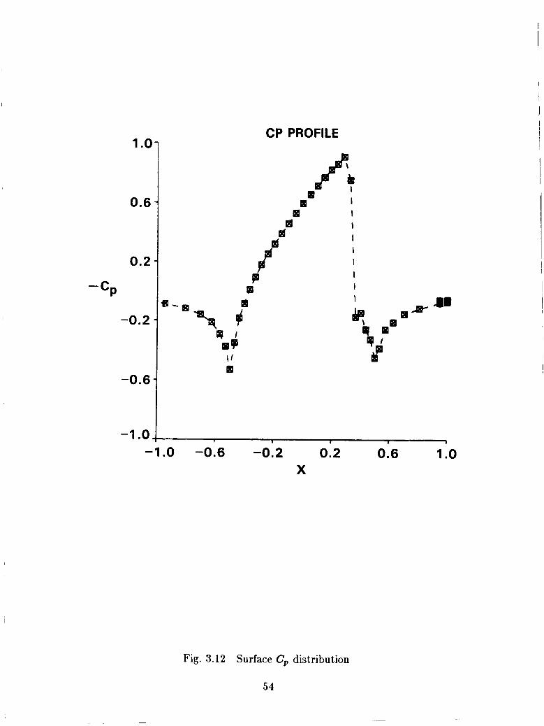
CP PROFILE 1 .o

0.6

0.2

- cP

-0.2

-0.6

9 1 ol

\ I Q

I I a I

d 1 I I 1

I P i I

-1 . o . . . , -1.0 -0.6 -0.2 0.2 0.6 1 .o

X

Fig. 3.12 Surface Cp distribution

54

m 0

N m F

m F

m

Table 3.1 Table of operation counts

55

v) (Y

0 m

0 v)

*

v) (Y

K (0 cc)

(Y

m m

0 v)

0 (Y K 0 cc)

m

00 cc)

0 v)

0 v)

d

Table 3.2 Table of computational times

56

Section 4.0 A NEW CLASS OF HIGH ACCURACY TVD SCHEMES

FOR HYPERBOLIC CONSERVATION LAWS

4.1 SUMMARY

A new family of high accuracy Total Variation Diminishing (TVD) schemes is presented in this section. Members of the family include the conventional second-order TVD upwind scheme, various other second-order accurate TVD schemes with lower truncation error, and even a third-order accurate TVD approximation. All the schemes are defined with a five-point grid bandwidth. The new algorithms are described for scalar equations, systems, and arbitrary coordinates. Selected numerical results are provided to illustrate the new algorithms and their properties.

4.2 INTRODUCTION

The new class of high accuracy Total Variation Diminishing (TVD) schemes can be defined essentially in terms of one parameter. By various choices of this parameter, one can obtain schemes with a wide range of accuracy including high accuracy (low truncation error) second-order schemes, the conventional second-order accurate upwind TVD scheme2 and even a third-order accurate TVD scheme. It is the purpose of this section to describe the new algorithm as it applies to scalar equations, to systems of equations, to arbitrary curvilinear coordinate systems, and to general control volumes (areas in two dimensions). In a paper by Osher and Chakravarthy'O, theoretical aspects of the new method are presented along with an extension of the construction to (2K- 1)-order accurate TVD schemes with a (2K + 1) point module, for K = 1,2,3,4,5,6,7. Three dimensional applications of the algorithm are also quite straight-forward but are reserved for Section 5. While the method is applicable to hyperbolic systems in general, we use the set of Euler equations of compressible inviscid flow for illustration.

We begin by presenting the governing Euler equations written in the Cartesian coordinate system in two dimensions along with background material on t,he connection between solutions to the Riemann Problem and first-order accurate upwind schemes. We next present the new algorithm for scalar equations, followed by illustrations of the accuracy of the various members of the new family in this simple case. The generalization to systems of equations is then discussed for both Cartesian and arbitrary curvilinear coordinate

57

systems. Various calculations using the Euler equations are then presented as illustrative examples.

In the description of the algorithm for systems of equations and for all the results presented here for the Euler equations, a high accuracy TVD algorithm based on Roe’s20 approximate solution of the Riemann Problem has been utilized for illustrative purposes and for computational efficiency. Other Riemann solvers such as Osher’s2’, the exact solution (the Godunov schemeIQ) can also be incorporated into the framework presented. Even the Split Flux scheme due to Steger and Warming2’ can be fit into the algebraic structure of the new family of algorithms even though it does not represent a Riemann solver4 (Section 2).

4.3 FIRST-ORDER ACCURATE UPWIND SCHEMES

This section describes the connection between solutions to the one-dimensional Rie- mann problem and upwind spatial discretizations of first-order accuracy. Throughout this section, the Euler equations are used for illustration of the algorithm for systems of equations. A unified boundary point treatment is also presented. The material presented in this section serves as a convenient background for the subsequent subsections and also makes this section reasonably self contained.

4.3.1 The Riemann Problem

We consider a system of hyperbolic conservation laws in two spatial Cartesian co- ordintes z and y, and time t ,

(4.3.1)

and its one-dimensional counterpart

q t + + s = o . (4.3.2)

Here, the dependent variable q and the fluxes f are m-vectors. Let qj and qj+1 denote the two piecewise constant states of a Riemann Initial Value Problem (IVP). Fig. 2.1 portrays (for m = 3) a possible wave structure in the exact solution to the Riemann problem which is made up of m + 1 piecewise constant states {qj+i/m,i = 0,. . . , m} which are separated by m wave families through which the states transition, abruptly across shock waves (genuinely nonlinear) and contact discontinuities (linearly degenerate),

58

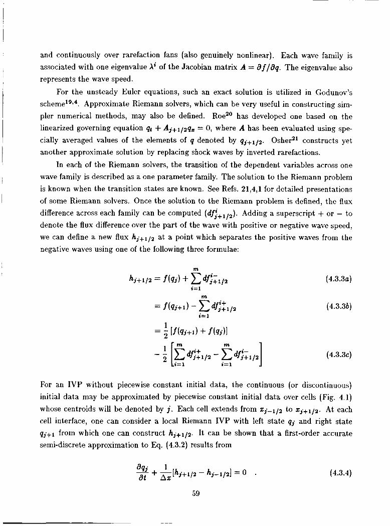
and continuously over rarefaction fans (also genuinely nonlinear). Each wave family is associated with one eigenvalue Ai of the Jacobian matrix A = af/aq. The eigenvalue also represents the wave speed.

For the unsteady Euler equations, such an exact solution is utilized in Godunov's s ~ h e m e ' ~ ~ ~ . Approximate Riemann solvers, which can be very useful in constructing sim- pler numerical methods, may also be defined. Roe20 has developed one based on the linearized governing equation qt + Aj+l /2~z = 0, where A has been evaluated using specially averaged values of the elements of q denoted by qj+1/2. Osher21 constructs yet another approximate solution by replacing shock waves by inverted rarefactions.

In each of the Riemann solvers, the transition of the dependent variables across one wave family is described as a one parameter family. The solution to the Riemann problem is known when the transition states are known. See Refs. 21,4,1 for detailed presentations of some Riemann solvers. Once the solution to the Riemann problem is defined, the flux difference across each family can be computed (dfj+,/,). Adding a superscript + or - to denote the flux difference over the part of the wave with positive or negative wave speed, we can define a new flux hj+1/2 at a point which separates the positive waves from the negative waves using one of the following three formulae:

m

i= 1 m

i= 1

m 1

(4.3.34

(4.3.3b)

(4.3.3c)

For an IVP without piecewise constant initial data, the continuous (or discontinuous) initial data may be approximated by piecewise constant initial data over cells (Fig. 4.1) whose centroids will be denoted by j . Each cell extends from ~ j - l / 2 to ~ j + 1 / ~ . At each cell interface, one can consider a local Riemann IVP with left state qj and right state qj+1 from which one can construct hj+1/2. It can be shown that a first-order accurate semi-discrete approximation to Eq. (4.3.2) results from

59

(4.3.4)

Adding and subtracting f(qj) to Eq. (4.3.4), and comparing appropriate pairs of h and f with Eqs. (4.3.3a-b), it is clear that Eq. (4.3.4) describes the influence of the right moving waves from the left and the left moving waves from the right on the centroidal grid point j under consideration; hence the name upwind scheme. The Riemann problem can thus be simply incorporated into first-order accurate discretizations. For multi-dimensional conservation laws, the one-dimensional Riemann problem with its simple solution is applied separately to each dimension in order to obtain independent discretizations of the flux derivatives in each spatial dimension, and the terms added up for the overall discretization. Any Riemann solver can be used including the three already mentioned. Even split flux methods (the one due to Steger-Warming” for example) can be fit into the same algebraic framework (Section 2) even though they are not Riemann solvers.

4.3.2 Boundary Conditions

The finite difference scheme can be extended to boundary points in a natural fashion by considering the local Riemann Initial and Boundary Value Problem (IBVP) at a boundary. Let us consider the left boundary shown in Fig. 4.1. In applying Eq. (4.3.4) to the boundary point, hj-1/2 is unknown because initial data is only prescribed upto the boundary and not into the exterior of the domain of interest. However, considering the definition for h based on Eq. (4.3.3b), it is obvious that the basic unknown quantities are the df~f,,,. If there are b families of waves moving from outside the boundary to the boundary (left to right) at the boundary, since each wave transition is defined by one parameter, an even more basic set of unknowns is the set of b unknown parameters corresponding to these wave families. We can then add a suitable set of b auxiliary boundary conditions. The b unknown parameters can then be chosen in such a fashion that the b boundary conditions are satisfied at the new time level (using the desired time discretization). This procedure gives rise to a boundary point treatment that is wholly compatible with the interior point differencing. Discrete conservation property is carried through all the way to the boundary point. Also, in this approach, flux differences for positive waves are defined at the cell interface just to the left of the boundary. These values are needed for higher-order discretizations one grid point to the right of the boundary and can thus be used to good advantage.

4.3.3 The Euler Equations

The Euler equations for two-dimensional inviscid flow correspond to the following

60

definitions of q, f l , and f2:

Density has been denoted by p, pressure by p, and the Cartesian velocity components by u and u. The total energy per unit volume is given by the expression

e=- 7 - 1

(4.3.6)

where 7 is the ratio of specific heats. Thus, pressure can be decoded from the dependent variables using

(4.3.7)

For one-dimensional problems, in z and t , fa can be set to zero along with u, and the last scalar equation component of Eq. (4.3.5) may be deleted.

4.4 THE NEW ALGORITHM FOR SCALAR EBUATIONS

We now describe the new family of high accuracy algorithm as it applies to scalar equations and that too for one spatial coordinate. For multi-dimensional scalar equations, the flux terms in each coordinate direction are treated in the manner described below and the uni-dimensional discretizations added up. A general control volume formulation can also be constructed, and is presented in a subsequent section. Rigorous theoretical inter- pretations of TVD schemes are applicable only to scalar nonlinear equations and systems of linear equations in one spatial dimension. The multidimensional implementations and extensions of the algorithms to nonlinear systems are not necessarily TVD14. However, the construction of these algorithms is straight-forward and the numerical results will be shown to be extremely good in all cases.

law: We begin by constructing the following representation of a semi-discrete conservation

(4.4.1)

Here, the quantity is the representation for numerical flux. With this notation, the numerical flux of the new family of TVD upwind schemes can be represented by the

61

addition of correction terms to the first-order accurate flux hj+l12:

(4.4.2)

The symbols-and=shown over the df denote flux-limited values of df and are computed as follows:

(4.4.34

(4.4.3b)

(4.4.3c)

(4.4.3d)

It is very desirable to build these high accuracy schemes around a first-order scheme which belongs to the class of E - ~ c h e m e s ~ ~ which will avoid expansion shocks or glitches4. In the above, the operator “minmod” is defined by

minmod [z, y] = sign(%) * max[O, min{lzI, y sign(z)}] (4.4.4)

and the parameter P is a “compression” parameter determined in the range given by

3 - 4 1 < p s - - 1 - 4

(4.4.5)

Normally, the maximum allowable value of P is used. Our purpose here is to illustrate the properties of this family of TVD schemes by applying the above discretization to the linear wave equation. Similar formulae can be easily developed to a system of nonlinear conservation laws, and will be presented in the next section.

The non-TVD or unlimited forms of the schemes in the new family can be obtained by replacing the 8 and @ terms that occur in EQ. (4.4.2) with their corresponding unlimited df values. The truncation error of the unlimited forms is given by

u

(4.4.6)

62

It is interesting to note that the T E (truncation error) is independent of the particular upwind-scheme used, i.e independent of h.

Particular schemes in the new family may be chosen by picking various values for the parameter 4. Some special cases are summarized in the following table (Table 4.1).

The T E shown in the last column corresponds to the corresponding unlimited forms. The names given to the TVD schemes are based on the names used in the literature for the corresponding unlimited schemes.

I

I

I I I

Underlying Scheme

Third-Order

Fully Upwind

Fromm’s

Low TE second-order

Central

No Name - 1/3

Table 4.1

Pmax 2nd order TE 4 0

1 A ~ 2 f l 2 + s ( 1 aza 2- 3 +&(A%) aza

5 - & ( A z ) ~ 3 1 2 f l

00 -ij(Az) aza

5/2 + ~ ( A z ) 2- aza

would be stable and TVD. However, for explicit time discretizations, for the fully discrete scheme to be TVD, there is usually a restriction on the magnitude of At that can be used.

When such a. time discretization is coupled with the new family of spatial discretizations, the time step restriction for the fully discrete scheme to be TVD is given by

I

(4.4.8)

63

and when the maximum permissible value for p is chosen (shown as Pmax in the previous table), the time step restriction is given by the Courant Number restriction

(4.4.9)

It must be noted that by using values of p smaller than Pmax, one can obtain larger bounds on the time step.

Some discussion of the “minmod” flux limiter is in order. The “minmod” operator is made up of two parts. When the two arguments x and y (see EQ. (4.4.4)) of the operator are of opposite signs, the value returned by the operator is zero. When the two arguments are of the same sign, the operator chooses z or y depending on which has a smaller absolute value. Let us consider this latter part of the “minmod” operator in some more depth. In Eqs. (4.4.3a-d), the flux-limited values of df are defined. The flux-limited value of df in some interval is defined by comparing the original unlimited value with its neighboring value after the neighbor has been multiplied by the “compression” parameter p. Assuming that the two values being compared are of the same sign, the “minmod” operator chooses the one whose absolute value is the smallest. Since the parameter p is quite large in all the particular schemes that we considered in the two tables, the flux-limited value returned most often will be the unlimited value itself. Thus, for most grid points (away from high gradient regions where the unlimited value of slope df can be much greater than the unlimited value of the neighboring slope), the TVD scheme which employs flux limiters will be locally identical to the corresponding unlimited scheme. Thus, the T E of the unlimited scheme is a good indication of the overall truncation error of the TVD scheme. So far we have considered two neighboring slopes with the same sign. At maxima and minima of the fluxes, the neighboring values of df can be of opposite sign. There, the “minmod” operator returns the value of zero. Thus, away from maxima, minima, shock waves and very strong gradients, the TVD scheme reduces to its corresponding unlimited scheme.

We conclude this subsection with some remarks on relevant work by other researchers. Bram van Leer3’ has in the past worked with Fromm’s scheme and also mentions the possible use of third-order accurate formulations. He has however not constructed flux- limited forms of the two in the manner shown here. There may also be some parallel between the Piecewise Parabolic method25 of Colella and Woodward and the high accuracy second-order formulations presented here.

64

4.4.1 Numerical Illustrations

We now discuss some numerical results. The new family of schemes was programmed for a linear wave equation with a source term which drives the solution to a time-asymptotic steady state.

qt + qz - A cos(7rz) = 0 . (4.4.10)

The semi-discrete TVD spatial differencing was combined with a multi-stage time differencing (which includes the simple one-stage scheme shown in &. (4.4.7)). The steady state exact solution of Eq. (4.4.10) is given by

g(z) = sin(lrz) (4.4.11)

The el norm per grid point and the loo norm (maximum absolute value) of the error between the numerical and analytic steady state solutions are shown for various schemes in Tables 4.2-4.7. The number of grid intevals used is denoted by J. The computations were performed in the interval -1 5 z 5 1. The solution has a maximum and a minimum in this interval. The numerical solution was assumed to be periodic outside this interval (the analytic solution also is) when those values were required to define the scheme near the end points of the interval. In this, the results presented here differ from those shown in Ref. 4 where a periodic extension w a s not used. Thus, the results of Ref. 4 have the influence of a nonperiodic boundary point treatment of lower accuracy.

From the tabulated entries, the order of global (using the e1 norm) and maximum local (e,) error can be computed as follows: Let the appropriate norm of the error for J intervals be denoted by E J . Then if 0 is the order of numerical error,

where J 1 a,nd 5 2 denote the number of intervals in each of considered.

In Table 4.2, results are shown for a first-order upwind

(4.4.12)

the pair of solutions being

scheme (x.+1/2 = hj+1/2)* From Tables 4.3-4.7, the following deductions may be made about the new low truncation error methods. The order of accuracy of all members of the new family are close to the order of the corresponding unlimited forms (Table 4.1) when measured from the l 1 norm. In the loo norm, all the schemes show second-order accuracy (even for 4 = 1/3). For any given number of grid points, the actual truncation error decreases as expected from Table 4.1 in the order 4 = -1 , -1/3,0,1/2,1/3.

65

20 30 40 60 80

0.14963+0 0.10133+0 0.76623- 1 0.5 1503- 1 0.38793- 1

0.29863+0 0.20253+0 0.15323+0 0.10303+0 0.77563- 1

Table 4.2 Error tabulation for 1st-order upwind scheme

J 20 30 40 60 80

0.15773- 1 0.7605 E- 2 0.44983-2 0.2 1043-2 0.12143-2

0.32163- 1 0.13943- 1 0.82743- 2 0.37213-2 0.20903- 2

Table 4.3 Error tabulation for 4 = -1, p = 2

J 20 30 40 60 80

0.97683- 2 0.43773-2 0.24903-2 0.11223-2 0.63733-3

~~ ~~

0.30273- 1 0.1060E- 1 0.74363-2 0.32743-2 0.18273-2

Table 4.4 Error tabulation for 4 = -1/3, p = 5/2

The behavior of the third-order formulation in the loo norm needs additional expla- nation. The “minmod” flux limiter returns a value of zero when neighboring slopes are of opposite signs. Thus, at a local maximum or minimum, the local truncation error must be

66

I

J 20 30 40 60 80

IIErrorll1 I I Error11 m

0.66693- 2 0.29253- 1 0.26673-2 0.10933- I 0.14423-2 0.72893-2 0.61733-3 0.32293-2 0.34173-3 0.1813E-2

Table 4.5 Error tabulation for 4 = 0, /3 = 3

J 20 30 40 60 80

I I Error1 I1 II Error11 00 0.37883-2 0.27723- 1 0.16373-2 0.11523- 1 0.80973-3 0.70273-2 0.342 13-3 0.31293-2 0.19373-3 0.17653-2

Table 4.6 Error tabulation for 4 = 1/2, /3 = 5

J 20 30 40 60 80

I I Error11 1 ll Errorlloo 0.36473-2 0.28173- 1 0.13653-2 0.11253- 1 0.55113-3 0.7 132 E- 2 0.17183-3 0.31753-2 0.731 2E-4 0.17863-2

Table 4.7 Error tabulation for 4 = 1/3, /3 = 4

of lower order. We actually expected this .local error to be first order for all members of the new family and thus we expected a first-order convergence rate in the maximum norm (&). However, the actually observed error in this norm showed second-order convergence.

67

Thus, the accuracy was even better than expected. The e1 norm is a measure of global error while the too quantifies maximum local error. If the local error is lower at just a few (and separate points) of the interval, the global accuracy can be maintained at the order of the majority value of local accuracy (the accuracy at most of the points) if the minority local error is not more than one order worse than the majority error. Since this condition is met for the third-order formulation, the accuracy in the e1 norm persists in being third order despite the second-order accuracy in the too norm. The other members of the family display second-order accuracy in both norms and could have continued to do so even if the error in the .too norm had degenerated to first order.

The local accuracy can degenerate at maxima, minima, boundary points (depending on the discretization), and also at sonic points for nonlinear equations (because of special treatment to remove glitches and satisfy the Entropy condition4). Formal truncation error analysis requires the existence of continuous derivatives of sufficient order. Sonic point treatment, flux-limiters, etc. can cause non-differentiability and thus make analysis more difficult. The scalar results presented here are supplemented by results for the Euler equations in a later section. There, each wave family is treated separately and thus formal accuracy analysis is even more difficult. In any case, based on the results presented above, it can be concluded that the use of the new family of low truncation error schemes will lead to substantial improvements in the accuracy of numerical solutions to hyperbolic equations. The third-order accurate scheme presented here is but the least accurate member of another family of very high order accurate TVD approximationslO. For K 5 7 , it is shown in Ref. 10 that TVD schemes of 2K - 1 order accuracy can be constructed using 2K + 1 grid points. The utility of such algorithms is yet to be demonstrated.

4.5 ALGORITHM FOR SYSTEM OF EULER EQUATIONS

We now describe the construction of the new family of high accuracy TVD schemes to the system of Euler equations. The algorithm for systems is a simple extension of the method for scalar equations. We begin by interpreting h, f , df, etc. to now be vector valued quantities corresponding to the dependent variable vector q and the vector fluxes f1 and fi. Let us consider one spatial dimension at a time and assume that h, f , df, etc. denote the appropriate quantities associated with the actual vector flux for that spatial dimension. From the algorithm to be described for one spatial dimension, the algorithm for more dimensions is simply constructed by adding the corresponding terms from each dimension.

68

4.5.1 Cartesian Coordinates

!

For scalar equations, there existed only one characteristic speed per dimension. For hyperbolic systems of equations, there are as many characteristic speeds as there are dependent variables. Considering the 2-t plane for example, the eigenvalues (characteristic speeds) of the corresponding Jacobian matrix are u - c, u, u, and t~ + c. Let us denote the individual flux differences by df’- and dfi+, where the superscript i corresponds to the number of the eigenvalue. Thus we define the df- and df+ used before to now mean the sum of the individual flux differences across the individual wave families.

m m

(4.5.1) S i

Based on the notation given above, the high accuracy numerical flux for systems of equations can be written as

h

fi.+1/2 = hi+l/2

(4.5.2)

N N N

As before, the symbols and shown over the df denote flux-limited values of df. But now these are defined field by field. Different families of high accuracy TVD schemes can be constructed by defining the positive and negative flux differences differently. For example, high accuracy TVD schemes can be derived based on the exact solution to the Riemann Problem (initial value problem with piecewise constant initial states), or approximate solutions to the Riemann problem such as Osher’s scheme or Roe’s method. Roe’s method (which must be used with an entropy fix mentioned elsewhere4) leads to a particularly simp!e construction fer the new family of upwind sckemes and is the recommended approach when computational efficiency is important. We now develop the particular family of high accuracy TVD upwind schemes based on Roe’s method of approximate solution of the Riemann Problem.

In Roe’s approach20, specially averaged cell interface values are determined for density,

69

velocities and enthalpy (h = 7p/ ( (7 - 1 ) p ) + (u2 + v2)/2)

I with the positive and negative parts of the eigenvalues defined by

from which the speed of sound c can be calculated as

(4.5.3)

Let R and L denote the matrix of right eigenvectors ri (as columns) and the matrix of left eigenvectors 1' (as rows), respectively, evaluated at the cell interfaces using Roe's average values for velocities and speed of sound. Then the individual differences in dependent variables across each wave family can be computed from

with ~ : . + i / a = Ij+1/2* (qj+1 - qj) (4.5.6)

In Eq. (4.5.6) and in what follows, it is tacitly assumed that R and L are orthonormal (Le. RL = I, where I is the identity matrix). The individual differences in fluxes across each wave family can be computed as the product of the eigenvalue and the corresponding dependent variable difference:

Now, df'- and dfi+ will be defined by

(4.5.8)

(4.5.9)

70

The physical meaning of the parameters ai can be identified by considering the state space of dependent variables. In such a space, the equation for dq’ (Eq. (4.5.5)) implies that the change dq is tangential to the right eigenvector for the wave family and that ai is a measure of the change of dependent variables across each wave family. We can now define a new parameter Q’ to be the product X’a’ and this parameter would be a measure of the change of fluxes across each family.

Now, we can define flux-limited values of Q to be analogous to the scalar definitions for flux-limited values of df using the “minmod” operator (see Eqs. (4.4.3)).

Then, the flux-limited values of the flux differences are defined to be

(4.5.1 la )

(4.5.1 1 b)

(4.5.1 1 c)

(4.5.11d)

It so happens that very simple expressions are available for the elements of R, L, and for the parameters ai. Thus, the coding of a TVD scheme for systems based on Roe’s approximate Riemann Problem solver can be very simple indeed. The expressions for R, L, etc. are given in a subsequent section in a form compatible with arbitrary curvilinear coordinates. The form for Cartesian coordinates can be obtained from these by suitably simplifying the expressions.

4.5.2 Arbitrary Curvilinear Coordinate Systems

Beginning with Eq. (4.3.1) and considering a transformation of variables of the type

71

we obtain the transformed conservation law

atq+ aef, + aJ2 = o

where - Q q = -

J - et & tu f1= JQ+ Jfl+ J f 2

f 2 = JQ+ Jfl+ J f 2 - rlt 5% r l Y

where, in turn, J is the Jacobian of the transformation:

(4.5.13) 1 I

(4.5.14)

(4.5.15) I

In Section 4.5.1, we used f to denote f1 or f2. Let us now use f to denote 7l or 7,. We note here that

f = f h , nz, nu) = f (Q, N) (4.5.16)

where n, and nu are either & / J and &,/J, or q , / J and 9y/J. The notation is appropriate because nz,y are the z! and y components of the normals to constant ( planes or constant 9

planes, when associated with (z,y or T,,~, respectively. Now, the semi-discrete conservation law (corresponding to Eq. (4.4.1)) can be defined as

(4.5.17)

Just as f is now a function of N, we expect dfif,12, etc. to be a function of Nj*l/2, and dfizll/z, etc. to be a function of N&*1/2, where Nj*1/2 and N k f l / 2 denote the normals to the constant j and constant k planes respectively.

Using the above, we can construct two types of numerical fluxes in arbitrary curvilinear coordinate systems. In the first version, we define each term on the right hand side of Q. (4.5.2) in terms of the metrics with the same subscript as the term under consideration. This implies, for example, that dfj+l/2 is computed using Nj+1/2 and d’j-1/2 is defined using Nj-1/2. This is an economical approach and has been used by the first author in all his results requiring transformation of dependent variables. In the second approach, all terms on the right hand side of Eq. (4.5.2) use the metrics Nj+1/2, whatever be the value of the subscript for the term under consideration. This translates into evaluating the Riemann solver several times at each cell interface, each time with a different set of

72

metrics, and can thus be quite time consuming. Nevertheless, the possibility is noted here for the record.

4.5.3 Eigenvalues and Eigenvectors

The actual expressions for defining the eigenvalues and eigenvectors are presented now for completeness. We express the eigenvalues and eigenvectors in terms of the generalized metrics n, and ny which define the x and y components of the cell-face normals. Let us define normalized values of these as

Then the eigenvalues of the Jacobian matrix c?f/aq, taken in increasing order are

~4 = (0 + c)dnz + ni

where 8 is the normalized contravariant velocity

n U = u i i x + v i i y .

For subsequent use, we also define

n v = v c i , - u i i y .

With this notation, the matrix L of left eigenvectors is given by

X x C c 2 C C

X X c c 2 C C

_ - _ - - - X q a o + c +-u-nu +-v+n, L =

_ - _-- H a +o + c +-u + ii, +-v - n,

(4.5.19)

(4.5.20)

(4.5.2 1)

(4.5.22)

+- +---i? x !la --u+iix X ( 1 c 2 C C

73

and the matrix R of right eigenvectors is given by

In the above, x = 7 - 1. The rows of L and columns of R correspond to the order of eigenvalues shown in Eq. (4.5.19). To construct the eigenvalues and eigenvectors for a

I vertical cell face in a Cartesian grid, one has but to set n, = f l and ny = 0. To construct

1 R = - 2

q2 c - + U + - 2c x 2c 2c 2c X -- Q2 O + - c Q2 -+p 92-p

1 - 1 - 1 - 1 - C C C C

U U U U

C C C C v , V v , V

C C C C

---fig - + F i g - + n,

- - ng - + f i x - - n, - + ng

fix - - I (4.5.23)

I

(4.5.24)

I 4.6 EULER RESULTS

Fig. 4.2 depicts the solution to a Riemann problem computed on an expanding grid with respect to which the waves are frozen in time. This effect is achieved in this case by assigning grid speeds proportional to distance from the origin (specifically, for the result presented, zr = 4.38 z). The solution plotted corresponds to r = 0.225. The excellent

contact discontinuities, and to track expansion fronts, when the mesh is aligned with these features. The problem solved corresponds to the left state given by p = l , p = 1,u = 0, and the right state given by p = 0 . 1 2 5 , ~ = 0 . 1 , ~ = 0.

The next few results are presented for nozzle flows computed using the quasi-one- dimensional assumption. Exact solutions to this case can easily be computed (available

I comparison obtained shows the ability of the numerical method to capture shocks and

74

I from most textbooks on gasdynamics). The numerical solutions are computed by adding the appropriate source terms to the one-dimensional equations. Figs. 4.3-4.5 display results I

I

for three types of flows. For the results, the area variation along the nozzle is 0.5 + x2.

For the shocked flow case, a couple of points around the shock wave were excluded from the reckoning of the norms.

norm and the loo norm of the error in pressure between the numerical and analytic solution are tabulated in Tables 4.8-4.10 f:x various schemes, for 40 grid intervals, and for the three types of flow fields shown in Figs. 4.3-4.5. Analysis of these results are complicated by boundary point treatment, sonic rarefaction operators, and shock waves. The results do show that the more accurate members of the new family (4 # -1) perform noticeably better than the conventional fully upwind formulation (4 = -1) . When a sonic rarefaction is part of the flow field, the formulation based on Fromm’s method (4 = 0) manifests superior accuracy. Restrictions of space and scope necessitate that a more detailed account of error analysis of the method for the Euler equations must

I

The average

I

I

I

I ~ be presented elsewhere.

4 -1 0

1/2 1/3

11 Error11 1 iI Errorll, 0.66973-3 0.26763-2 0.19143-3 0.30943-3 0.24963-3 0.14933-2 0.21003-3 0.10263-2

Table 4.8 Error tabulation for smooth transonic flow

4 -1 0

1/2

11 Error11 1 I I Errorlloo 0.44233-3 0.81 13E-3 0.17683-3 0.29293-3 0.9714E-4 0.35323-3

I Table 4.9 Error tabulation for fully supersonic flow

1/3 I 0.13023-3

75

0.24173-3

I 76

Table 4.10 Error tabulation for shocked flow

-1 0

1/2 1 /3

Figs. 4.6a-b show results for a sphere in a supersonic stream (Mm = 2.0). An un- clustered grid of 30 (circumferential) by 20 (radial) grid intervals was used. Mach number contours are shown in Fig. 4.6a and surface pressure distribution in Fig. 4.6b along with a comparison with results of Lyubimov and R u s a n ~ v ~ ~ .

Multiple reflections of an oblique shock wave are shown in Figs. 4.7a-b ( M , = 2.0, incident shock angle = 32.6”, 120 x 20 interval grid). Pressure contours are shown in Fig. 4.7a. Pressure profiles at y = 0 (square symbols), y = 0.5 (circles), and y = 1 (triangles) are shown in Fig. 4.7b.

Good shock “capturing” ability is demonstrated by these calculations for both normal and oblique shock waves. The two-dimensional calculations made use of relaxation methods which can be and have been developed for TVD schemes5. The new higher accuracy formulation was incorporated into the framework developed in Ref. 39 for the earlier fully upwind formulation. Even though only individual members of the new family of schemes have been used in the results presented here, the good quality and accuracy of the results is a common feature of all the low-truncation-error formulations in the new family.

0.59713-3 0.26773-2 0.17263-3 0.11653-2 0.4 8 70 E- 3 0.31193-2 0.32923-3 0.21913-2

4.7 REMARKS

A new family of high accuracy TVD schemes has been presented in detail for scalar equations and the Euler equations. The new method offers substantially better accuracy for negligible additional computational effort when compared to the earlier generation of second-order accurate TVD schemes. Computer programs based on the new formulation are being routinely used for both two and three dimensional computations.

The new higher accuracy formulations are excellent candidates for discretizing the inviscid terms of the Navier-Stokes equations”. When k-E (two equation) turbulence models are used, the convection terms of these can also be approximated using the new TVD formulation18.

TVD schemes based on the high-accuracy formulations presented here offer improved accuracy and reliability-t he latter by avoiding spurious oscillations. They are excellent discontinuity “capturing” methods. They can be used in Navier-Stokes solver. They follow the physics well-they are upwind biased, satisfy the Entropy condition (more or less), and avoid unphysical “wiggles”. They permit the use of a wide variety of solution procedures- explicit, implicit, relaxation, etc. In short, they are a versatile set of tools that can enrich the productivity of many an engineer and scientist.

77

CELL INTERFACE RIEMANN PROBLEMS

---

INTERIOR DOMAIN

Fig. 4.1 Local Riemann problems

78

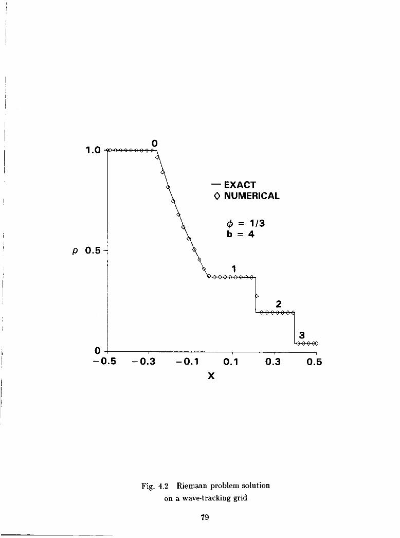
I

1 .o

p 0.5

0

0

- EXACT 0 NUMERICAL

-0 .5 -0.3 -0.1 0.1 X

0.3 0.5

Fig. 4.2 Riemann problem solution on a wave-tracking grid

79

1 .oo

0.800

0.600

P

0.400

0.200

0.000E + 00

-EXACT B NUMERICAL

4 = 0 b = 3

-0.333 -0.667E-01 0.200 0.467 0.733 1-00

X

Fig. 4.3 Smooth transonic flow in a quasi-one-dimensional nozzle

80

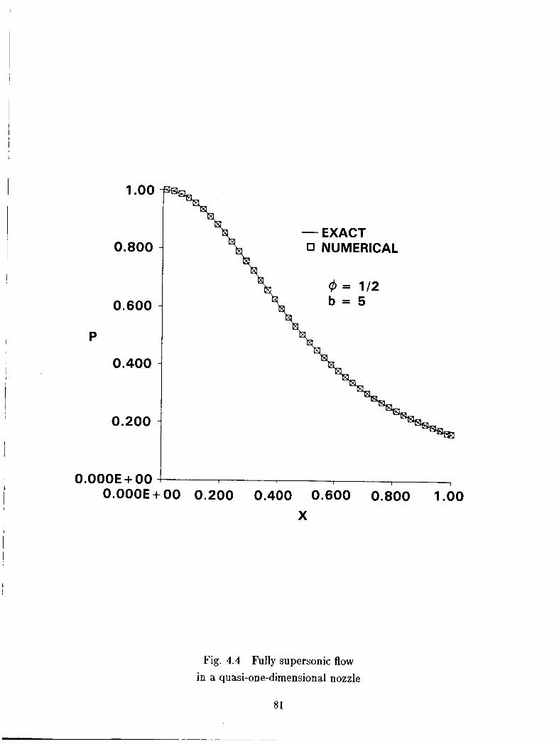
P

1 .oo

0.800

0.600

0.400

0.200

- EXACT 0 NUMERICAL

i $ = 112

\ b = 5

0.000E + 00 4, 0.000E+00 0.200 0.400 0.600 0.800 1.00

X

Fig. 4.4 Fully supersonic flow in a quasi-one-dimensional nozzle

81

,

P

0.800

0.600

0.400

0.200

0.000E + 00 1 1 I

-0.333 -0.667E-01 0.200 0.467 0.733 1.00 X

Fig. 4.5 Transonic flow with shock wave in a quasi-one-dimensional nozzle

82

2.00

1.60

1.20 Y

0.800

0.400

0.000E + 00

.6

-2.00 -1.60 -1.20 -0.800 -0.400 0.000E+00

X

Fig. 4.6a Supersonic flow past sphere

83

6.00

4.80

3.60

P

2.40

1.20

0.000E + 00

- LY UBlMOV & RUSANOV PRESENT NUMERICAL

0

0.000E+00 18.0 36.0 54.0 72.0 90.0 e

Fig. 4.6b Surface pressure distribution

84

Y

3.08-

P

0 0 1.6 3.2 4.8 6.4 8.0

X

Fig. 4.7a Multiple reflections of oblique shock: pressure contours

2.56-

X

Fig. 4.7b Pressure profiles

a5

Section 5.0 AN EULER SOLVER FOR THREE-DIMENSIONAL

SUPERSONIC FLOWS WITH SUBSONIC POCKETS

5.1 SUMMARY

The algorithmic framework described in the previous sections has been used to develop a new finite-difference scheme that efficiently solves the Euler equations for three- dimensional inviscid supersonic flows with subsonic pockets. The technique utilizes planar Gauss-Seidel relaxation in the marching direction and approximate factorization in the cross-flow plane. It is a unified formulation based on the unsteady Euler equations: an ‘infinitely large’ (‘infinitely small’ reciprocal of) time step is used in parts of the flow- field where the component of velocity in the marching direction is supersonic-here the Gauss-Seidel sweeps are restricted to the forward direction only and the procedure reduces to simple space-marching; a finite time step is used in parts of the flow-field where the marching component of velocity is subsonic-here backward and forward Gauss-Seidel sweeps are employed to allow for upstream and downstream propagation of signals, and a time-asymptotic steady state is obtained. The discretization formulae are based on finite- volume implementations of high accuracy (up to third order) Total Variation Diminishing formulations. The fully general coordinate treatment used permits the use of arbitrary marching fronts (rather than just planes perpendicular to an axis, spherical fronts, etc.). Results are presented for an analytically defined forebody, a twisted-cone inlet spike, a realistic fighter configuration, and the Space Shuttle.

I

I

5.2 INTRODUCTION

For fully supersonic flows, an efficient strategy for obtaining numerical solutions is to employ space-marching techniques. Realistic high speed flight vehicle configurations often give rise to subsonic pockets even though they fly at supersonic speeds. For such predominantly supersonic flows, a hybrid approach is suitable: a space marching technique for the supersonic parts and a relaxation technique for the subsonic parts. Such a hybrid approach has been developed for potential flows by Shankar, Szema et a140-41-4a. For the Euler equations, however, the hybridization is conventionally achieved by coupling separate space-marching and time-marching codes, each with disparate grid systems, etc. Here, we present a unified approach for efficiently solving the Euler equations for three-dimensional

86

supersonic flows with subsonic pockets. The aim is to develop an Euler solver as versatile as the potential flow so1vers40741~42 in treating complex and realistic aircraft, space shuttle, and other types of flight vehicle configurations. By solving the Euler equations, however, we hope to be able to compute a wider range of flows with stronger shocks, rotational slip streams, etc. which void the irrotationality assumptions built into the potential flow simulations.

The new approach utilizes finite-volume implementations of high accuracy (up to third order) Total Variation Diminishing (TVD) discretizations and are thus expected to be more accurate and reliable than other Euler space-marching and time-marching techniques based on central difference approximations. In contrast to these latter methods, there are no parameters in our approach for fine-tuning numerical dissipation for every case. Numerical oscillations are, for the most part, eliminated by using TVD scheme based discretizations.

The new approach is based on the unsteady Euler equations. However, in the supersonic parts of the flow (where the velocity component normal to the cross-flow plane that identifies the local marching direction is supersonic) an ‘infinitely large’ time step (which implies an ‘infinitely small’ reciprocal of time step) is employed. This makes the transient terms of the discretized unsteady equations vanish. In subsonic parts of the flow, a finite time step is employed and the steady-state is approached as a time-asymptote.

The new solution approach is based on a planar Gauss-Seidel relaxation method coupled to approximate factorization in the cross-flow plane. In supersonic parts of the flow- field, the Gauss-Seidel method is restricted to forward sweeps and thus the solution procedure reduces to a simple marching technique. In subsonic parts, both forward and backward sweeps are used along with the finite time steps mentioned earlier. Stability of such an approach is guaranteed by the diagonal dominance resulting from using TVD discretizations in the marching direction in the transonic parts of the flow-field. This is a crucial difference between conventional hybrid Euler solvers and the new approach. In conventional approaches, space-marching and time-marching techniques must be applied in overlapping regions for stability. In the new mified approach, there is no need for overlap.

In the following sections, we describe the new method in detail. We first cast the equations in finite-volume discrete conservation law form. Then we explain how the volume and the metrics are evaluated. This essentially completes the treatment of geometry and we proceed next to the details of the algorithm. TVD dlscretizatims are exp!ained first. Then the marching/relaxation procedure is described. This covers th? use of approximate factorization in the cross-flow plane, the reduction of the Gauss-Seidel procedure to a marching procedure in supersonic zones, etc. The boundary point treatment is also explained briefly.

In the results section, calculations for an analytically defined forebody are presented first to illustrate some features of the new algorithm. Results for many conical flow cases have also been obtained but are presented elsewhere43. Next, results for a twisted-cone inlet spike are shown. Then, results are presented for a realistic fighter aircraft configuration with fuselage, canopy, wing, nacelle and vertical tail. Finally, we conclude by presenting results for the Space Shuttle Orbiter configuration.

5.3 FINITEVOLUME FRAMEWORK

In this section, we describe the finite-volume framework chosen to implement the algorithm. We start by introducing the semi-discrete conservation law form and associating it with a finite-volume formulation of the geometry. Then we provide detailed formulae for the evaluation of the cell volume and cell-face normals.

5.3.1 Semi-discrete Conservation Law

We begin with the conservation law form of the unsteady Euler equations in the Cartesian coordinates z,y,z, and time t

Qt + E, + Fsr + G, = O (5.3.1 a)

where the dependent variable vector Q, and the fluxes E, F , and G are given by

(5.3.1 b )

In the above, pressure is p, density is p, Cartesian z, y, z velocity components are u, u, W ,

and the total energy per unit volume is e computed from e = p / ( 7 - 1) + p ( u 2 +u2 +w2)/2.

Assuming a time invariant grid, under the transformation of coordinates implied by

88

Eq. (5.3.1) can be recast into the conservation form given by

I

where

where, in turn, J is the Jacobian of the transformation

(5.3.34

(5.3.33)

Associating the subscripts j, k, 2 with the (, 7, directions, a numerical approximation to Eq. (5.3.3a) may be expressed in the semi-discrete conservation law form given by

h h

(Gj ,k , l ) r + ( ~ j + 1 / 2 , k , l - ~ j - l / 2 , k , l ) h + (p j ,k+1 /2 , l - pj ,k- l /? , f ) (5.3.4)

h h + (Gj,k,f+l/a - Gj,k,f-1/2) = 0 h h h

where E , F , G are numerical or representative fluxes at the bounding sides of the cell for which discrete conservation is considered, and Q j,k,i is the representative conserved quantity (the numerical approximation to g ) considered conveniently to be the centroidal or cell-average value. The half-integer subscripts denote cell sides and the integer subscripts the cell itself or its centroid. In Fig. 5.1, the eight vertices of one computational hexahedral cell are identified by numerals 1 through 8. These must be associated with the appropriate j , k, 1 triplets:

h

1 j - 1/2, k - 1/2,1- I ,‘2

2 = j + 1/2,k- 1/2,1- 1/2

3 G j - 1/2,k+ 1/2,1- 1/2

4 f j - 1/2,k- 1 /2 , l+ 1/2

5 = j + 1 / 2 , k + 1 / 2 , 1 - 1 / 2

6 r j - 1/2,,k+ 1 /2 , /+ 1/2

7 r j + 1/2,k- 1 /2 , l+ 1/2

8 j + 1/2, k + 1/2,1+ 1/2

(S.3.5)

89

In the following, subscripts easily understood by implication will be dropped for brevity. I

The semi-discrete conservation law given by h. (5.3.4) may be regarded as represent- ing a finite-volume discretization if the following associations are made:

where V is the volume of the cell under consideration;

I (5.3.6 b )

In the above, nz,y,z are the z, y, z components of the representative normals to the surface formed by the four points a, b, c, d implied in nz,g,8(a, b, c, d ) . Four points do not necessarily lie in one plane and therefore the components nz,y,z refc.:. to representative values for an equivalent single plane.

The evaluation of the volume and metrics (cell-face normals) are now presented in the following subsections. The evaluation of the representative flux is presented in the next major section.

5.3.2 ComDutation of Cell Volume

(5.3.7)

3

k

I

A- /

/

L

1 1 4

8

7

Fig. 5.1 Computational finite-volume cell

91

Then, referring to Fig. 5.1 again, the volume of the hexahedron is computed as a sum of

the six individual tetrahedra that constitute it.

(5.3.8)

It is of interest to note that such a formula will result in the proper evaluation of volume even when some of the faces of the hexahedron collapse t:, a line or a point.

5.3.3 Computation of Cell-Face Metrics (Normals)

In Eq. (5.3.6b), cell-face normals were introduced. Each cell face is identified by four vertices not all of which are necessarily on a single plane (three points being sufficient for defining a plane). In our approach, we allow for this and also for some of the faces to collapse to an edge or even a point. Computationally, we will always identify a face by its four vertices a, b, c, d expressed in the j , k, I subscript system. Physically, some or all of the four vertices may lie at the same z, y , z location.

The cell-face normals are evaluated as

(5.3.94

(5.3.93)

where, in turn, s corresponds to z or y or z , and 1 and 2 correspond to u or b or c or d . The first term in each of the definitions is respectively one half of the z, y , or z component of the cross product of the vector from u to b with the vector from b to c. The second term in each definition is correspondingly one half of the z, y , or z component of the cross product of the vector from c to d with the vector from d to a. A cross product of two vectors lies along the direction of the normal to the two vectors. In the present situation, the two vectors are connected. Therefore, such a normal also defines the direction of the

9 2

normal to the plane containing the two vectors. One half of the cross product, of connected vectors also has a magnitude equal to the area of the three dimensional triangular planar shape defined by the two vectors. Thus, while &,y,z/J, qz,y,z/ J , (z,y,z/ J define the x , y, z

components of the normals (not unit normals) to the local tangent plane to the constant t , q , ( surfaces respectively, the associated quantities (nz,y,z) j ,k , l define the components of the normals to the local constant j , k, I planes.

5.4 TVD DISCRETIZATION

n h h

In the last section, the numerical or representative fluxes E , F , G were introduced. These fluxes are so named because they approximate the real fluxes E , F , G to the required order of accuracy. The actual fluxes appearing in the governing partial differential equations depend on the metrics <s,y,z/J, q z , y , z / J , (z,y,z/J and correspondingly, we allow the numerical fluxes to depend on the numerical metrics (the cell-face normals). In the last section we did point out the link between the metrics and the components of the cell-normals, but the numerical flux was not defined there. The latter task is the subject of this section.

---

We employ an upwind-biased scheme in our approach in such a fashion as to essentially eliminate numerical or spurious (unphysical) oscillations while, at the same time, achieving high accuracy. In order to describe this type of discretization, we first mention the underlying upwind scheme used in terms of the corresponding approximate Riemann Solver, and then expand upon how high accuracy and the TVD property are built in. More details on these and related topics may be found in Refs. 6 and 4 and in references cited therein.

5.4.1 Roe’s ADDroximate Riemann Solver

The Riemann Solver is a mechanism to divide the flux difference between neighboring states (between Qm and Qm+l for e.g.1 into component parts associated with each wave field. These can in turn be divided into those that correspond to positive and negative wave speeds. When we compute the numerical flux at the cell face at rn + 1/2 using various combinations of fluxes and positive and negative flux differences, in the finite- volume formulation, we will only use the ceii-face normals defined at m + 112 in ail the terms contributing to that representative flux. The actual fluxes E, F , G , when evaluated with the metrics equated to cell-face normals, can all be written in the same functional form given by

E , F , G = f ( Q , nztny, n z ) = f ( Q , N) (5.4.1)

---

---

93

where the appropriat,e values of n,, nu, n, are used and N denotes the set of those normals. Using such notation, it is possible to present the necessary algebra very concisely.

Let us first denote the Jacobian matrix of the flux f with respect to the dependent variables Q by a j / a Q . This Jacobian can also be called the coefficient matrix. Let us denote the eigenvalues of t)he coefficient matrix by Ai and the corresponding left and right eigenvectors by ti and ri, respectively. The matrix formed by the left eigenvectors as its rows is then called the left eigenvector matrix L and the matrix of right eigenvectors com- prising right eigenvectors as its columns is R. For our purposes, we choose an orthonormal set of left and right eigenvectors which implies that LR = RL = I, the identity matrix. In the above, the superscript i has been used to denote the association of the i-th eigenvalue with its corresponding eigenvector. Each eigenvalue is also associated with its own wave field.

The underlying upwind scheme is based upon Roe’s approximate Riemann solver20. In this approach, cell interface values of density, velocities, and enthalpy (h = rp/((r - 1)p) + (u2 + ua + w2)/2) are computed using a special averaging procedure:

where m = J’ or k or 1. From the above, the speed of sound can be computed from

(5.4.2)

Knowing (u, u, w, c ) , + ~ / ~ , the eigenvalues and orthonormal set of left and right eigenvectors corresponding to a cell face can be computed. These may be denoted by

(5.4.4)

At each cell face, the positive and negative projections of the eigenvalues may be defined by

(5.4.5)

94

In order to help Roe's Riemann Solver avoid expansion shocks, only at sonic rarefactions (Ai(Qm, Nm+l/2) < 0 < Ai(Qm+l, Nm+li2)), the corresponding positive and negative projections are redefined as

(5.4.6)

For the sake of completeness, detailed formulae for the eigenvalues and the eigenvector matrices are now presented. Defining the contravariant velocity by

- U = ,n,u + nyv + n,w , (5.4.7)

the eigenvalues are given by

Defining

and

6 = (u2 + ua + d ) / 2 ,

(5.4.8)

(5.4.9)

(5.4.10)

the left and the right eigenvector matrices are given in Table 5.1 and Table 5.2 respectively.

5.4.2 High-Accuracy TVD Schemes

We can construct upwind-biased schemes of varying accuracies using the basic ingre- dients given in the last subsection. Here, we present a family of schemes based on the preprocessing approach4. Let us now define some convenient variabies as an intermediate step before defining the numerical flux corresponding to a high-accuracy TVD scheme. First, we define a parameters which are a measure of the change in dependent variables across the corresponding wave family and therefore are a measure of the slope between neighboring states. In the following, the superscript i corresponds, as usual, to the i-th

95

[ e r + C n,u

-nzu + nzw

+nyu - n,u

+nzu - n,w

[et9 C - ii,u

- ngu - n,w] /&i

[-Eu C

-6.1 /&i

nvU 7 - 1

C

+n,

7 - ln,u C

I

-nu

7 - ln,U C

[-eu C

+n.] /di

[-eu C

- n,] Id5 J

- lA,U C

[-Ew C

- n, J

7- ln ,w C

-Fi,

7 - ln,w C

Table 5.1 The left eigenvector matrix L

eigenvalue and i-th eigenvector. The subscripts 1, 2, and 3 are just labels to differentiate

between the three different types of a parameters.

(5.4.11)

96

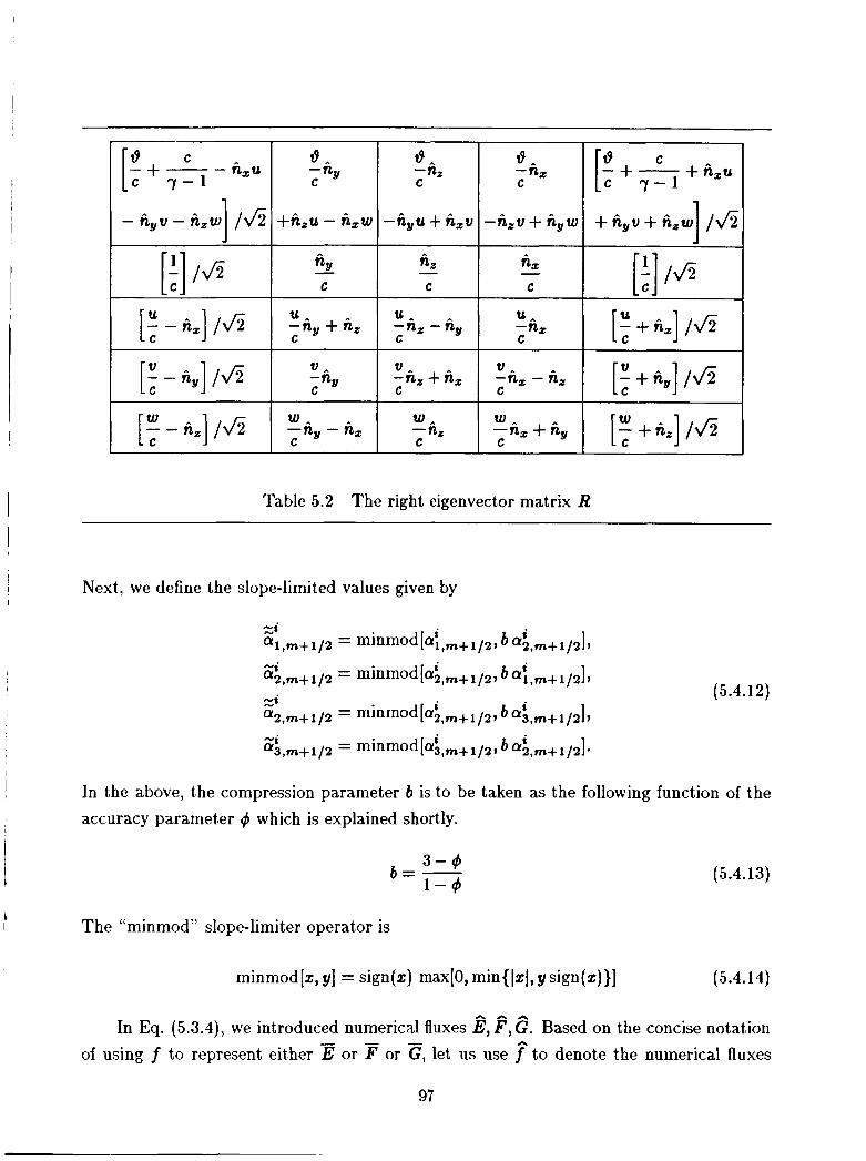
0 -

-fi,u + fi,w

- n, C

C -+- + n,u [* c 7 - 1

+ n y u + A,w] /&I +fi,u - fi,w 1 -nyu + fi,u

C C C I

1 [I-B,]/Jz u - -n, - n, C

W

C -n, + fi,

Table 5.2 The right eigenvector matrix R

Next, we define the slope-limited values given by

(5.4.12)

In the above, the compression parameter b is to be taken as the following function of the accuracy parameter 4 which is explained shortly.

3 - 4 1 - 4

b = - (5.4.13)

The “minmod” slope-limiter operator is

minmod[z, y] = sign(%) max[O, min{ IzI, y sign(z)}] (5.4.14)

h h h

In Eq. (5.3.4), we introduced numerical fluxes E, F , G. Based on the concise notation or F or z, let us use 7 to denote the numerical fluxes of using f to represent either

97

E or P or G. We can then write down a family of TVD schemes as follows in terms of the previously defined c; parameters (with the subscript m + 1/2 dropped from these for convenience) :

I

~

h

fm+l /2 = hm+1/2

1 - 4;) + c (""z; 4 + - 4 m+ 1 /ark+ 1 /2

t (5.4.15) I

The first term on the right hand side of Q. (5.4.15) defines a first-order numerical flux and is constructed from

(5.4.16)

i

i

The remaining terms on the right hand side of Eq. (5.4.15) define correction terms that upgrade the accuracy. For use in the next subsection, we define

( 5.4.1 7)

It is interesting to note that in all the above formulae used to define the numerical flux at m + 1/2, the eigenvectors and eigenvalues are only necessary at the corresponding cell interface. Therefore, the only geometry information used corresponds to the cell-face normals at rn + 1/2. The solution variables Q are sampled between the centroidal points m - 1, m, rn + 1 , m + 2 when the various a parameters are defined.

The parameter 4 defines schemes of varying accuracy. The notations a"' and :* have been used to define slope-limited values of the a parameters. If we replace these by their unlimited values, we obtain schemes whose truncation error in one-dimensional steady- state problems on uniform grids is given by

(5.4.18)

98

Here, the truncation error refers to the difference between the centroidal value of the numerical solution and the average value of the exact solution in that cell. The choice of 4 = 1/3 results in a TVD scheme based on an underlying third-order scheme. The choice of 4 = -1 results in a TVD scheme based on the fully upwind second-order accurate formulation. Fromm's scheme arises when 4 = 0.

5.4.3 TVD Schemes and Diagonal Dominance

In the next section, a procedure is presented to solve the finite difference equations resulting from the TVD discretization of the space differencing terms. In supersonic zones, the method reduces to a simple marching scheme, while in subsonic zones it becomes a relaxation approach and both forward and backward sweeps are employed along the marching direction. In order for such a relaxation approach to be stable, a sufficient condition is the diagonal dominance of the underlying finite difference scheme. This diagonal dominance can be shown to exist for TVD discretizations. For more details, the reader is referred to Ref. 5 and Section 3.

5.5 THE SOLUTION PROCEDURE

We begin this section by considering an implicit time discretization coupled with the TVD space discretization discussed earlier in terms of the corresponding numerical flux terms.

(5.5.1)

n+ 1 + ( G + l / 2 - L / a ) = 0

Here, n is the index in time and AT is the time step. In what follows, we will consider the iinearization oi the above nonlinear set of finite difference equations. Then we will simplify the algebraic solution procedure by approximately factorizing the implicit operator ih the cross-flow plane (which is a plane in only computational coordinates-constant j plane). The marching direction is along j. We will further specialize the scheme for the two cases of supersonic and subsonic velocity components in the marching direction.

99

5.5.1 Linearization

Let us linearize Eq. (5.5.1) about a known state Q = q' using a Newton procedure to obtain a better approximation q'+' to Q"+'. Here, s is a subiteration index. Defining I

1 i

(5.5.2)

we can describe the Newton procedure by I

1 (5.5.3)

a - (AjE+ AkP + A1G) A'q =

Ar aq [ - I + V

- 9") + AjE(q') + AkP(9') + AlG(q')

We next simplify the left hand side by defining an approximation to the true linearization. Towards this goal, we consider only a first-order accurate scheme (based on the first-order numerical flux h) for the left hand side while we include the full high-accuracy scheme on the right hand side. Even so, when the subiterations converge, the right hand side is satisfied to the desired degree. Next we assume that the eigenvalues and eigenvectors are not functions of q. Finally, we observe that

m= j,k, l

m= j,k,l i m= j,k, l i

because, in expanding Eq. (5.5.4) using Eq. (5.4.16), we find that

(5.5.4)

(5.5.5)

100

when the cell-face normals are evaluated using the formulae given in Eq. (5.3.9). Using the above, Eq. (5.5.3) is simplified to

V - A'q AT

where

(5.5.6)

(5.5.7)

(5.5.8)

in which A is the diagonal matrix whose diagonal elements are A' and [A[ is the diagonal matrix whose diagonal elements are [A' ] .

5.5.2 Planar Gauss-Seidel Relaxation

Even after the many simplifications leading to Eq. (5.5.6), it is obvious that more algebraic simplification is needed before a computationally feasible and efficient solution procedure is obtained. This is because l?q. (5.5.6) signifies a system of equations which links every point j , k, I with its six neighbors j + l , j - 1, k + 1, k - 1, I + 1, I - 1 in such a fashion that the left hand side of Eq. (5.5.6), when considered for all grid points, is a huge (even thnugh sparse) matrix whcllse bandwidth is also very large. Of course, for supersonic flows, a fully upwind difference approximation arises in the j direction and the dimensionality is reduced because the left hand side does not link j with j + 1. However, with our expressed aim of developing a method for subsonic pockets also, it is necessary to coosider the czse wheii j is linked with both its neighbors j - 1 and j + 1. In such a case, a direct Gaussian elimination procedure for the matrix system of equations would be unacceptably expensive. Therefore, instead of a direct elimination procedure, we seek to obtain an efficient relaxation solution to Eq. (5.5.6). We choose a planar Gauss-Seidel procedure by retaining all terms of the left hand side except the off-diagonal terms in

101

I

j (those terms that multiply A'qj*1). That such a procedure will be stable for TVD discretizations was discussed in subsection 5.4.3 and in the references cited therein.

The planar Gauss-Seidel procedure can be written as

1

1 V

+ V ~ ~ 1 / , ( A 8 Q 1 + 1 - A'qd

= -[Right Hand Side of b. (5.5.3)] . Denoting

(5.5.9)

(5.5.10)

we can rewrite Eq. (5.5.9) as

(5.5.11)

= Li-'[Right Hand Side of Eq. (5.5.3)] . V Of course, when the relaxation cycles denoted by superscript s converge to the desired extent, Abq = 0, and the full accurate formulae of the right hand side will be satisfied to a corresponding degree.

5.5.3 Approximate Factorization in the Plane

While EQ. (5.5.11) defines an algebraic set of equations whose dimensionality is one order less than that of EQ. (5.5.9), it is still too huge to be tackled by an elimination algorithm. Therefore, we will now further reduce the dimensionality by approximately factorizing the left hand side of Q. (5.5.11) to result in

(5.5.12)

= Lz-l[Right Hand Side of l3q. (5.5.3)] . V

102

The actual sequence of steps to solve Q. (5.5.12) can be chosen so that 2-l need not actually computed and only A is needed. For this purpose, we solve, in order, the equations

1 V

= --[Right Hand Side of Eq. (5.5.3)]

and

(5.5.13a)

(5.5.13b)

with ij being a temporary storage variable. Let us summarize the solution procedure developed in Eq. (5.5.13) for just one con-

stant j plane. Equation (5.5.13a) must be solved for all k-varying lines (for all I ) . Then Eq. (5.5.13b) must be solved for all I-varying lines (for all values of k). However, each k- varying or I-varying line is associated with only a one-dimensional block-tridiagonal system of algebraic equations whose block matrices are 5 x 5. These two steps only constitute one cycle of the Gauss-Seidel iterations and that too for only one constant j plane. The planar Gauss-Seidel procedure requires that one constant j plane is updated at a time. When the neighboring j plane is updated next, the latest available values of the update variables q are used in the right and left hand sides. The j sweep strategy will be specialized for supersonic and subsonic flow regions in what follows.

5.5.4 Pronramminer Notes

We store grid information at two planes (grid-planes 2 and 3) which describe the j boundaries (j - 1/2 , j + 1/2) of one plane of cells. Let the centroids of these cells be denoted as solution-plane 3. Array storage is provided for dependent variable planes (solution-planes) 1,2,3,4,5. As the sohtion Is marched, the contents of the grid-p!me and solution-plane arrays are updated by replacing them with neighboring values or by the planar Gauss-Seidel algorithm.

Let us consider the very first marching sweep now. We begin by initializing the two grid planes and the dependent variables at solution-planes 1 aob 2. ??e are Interested in updating the solution at plane 2. We first set the solution at planes 3, 4 and 5 to be equal to the values at solution-plane 3. After one or more subiterations for solution-plane 3, we shift our attention to the next j-plane. Grid-plane 2 is replaced with the contents of grid-plane 3. Grid-plane 3 nodal values are stored on auxiliary storage for later use.

103

New values for grid-plane 3 are generated by grid generation procedures or read in from auxiliary storage initialized previously. Similarly, solution-plane 3 is saved on auxiliary storage for subsequent processing. Solution-plane 1 is replaced by contents of solution- plane 2, and plane 2 is then replaced by contents of plane 3. Solution-planes 4 and 5 are set to the values at plane 3 and the marching proceeds.

If more than one subiteration is to be performed in the first marching sweep, the grid information is not updated for the subsequent subiterations. Solution-planes 4 and 5 are reset to values at solution-plane 3 after the previous subiteration and the next subiteration is processed. Solution-plane 3 values are not set to solution-plane 2 values for the second and subsequent subiterat ions.

For fully supersonic flows, a fully-upwind, not-flux-limited differencing scheme is used. Thus, the values set for solution-planes 4 and 5 are actually not used at all. Forward marching is enough. Even first-order upwind scheme in the j-direction and one subiteration per marching plane are also often enough. A small value is input for the reciprocal of time step. Accuracy of approximate factorization for any time step size is maintained due to reasonable marching step size (distance between j grid planes).

Subsonic regions could develop as a result of gradual compression (for e.g., around canopies) or abrupt transition through a shock wave (for e.g., in front of a blunt nosed object in an oncoming supersonic flow). In such regions, a larger value is chosen for the reciprocal of time step. The solution is marched forward using one or more (usually a maximum of two) subiterations by conforming to the procedure outlined above for the first, marching sweep. Then, a backward marching sweep (or even another forward marching sweep) is performed. For all sweeps (forward or backward) after the first, solution planes are filled with previous sweep solution values before updating using subiterations. Shifted replacements of solution-plane values of dependent variables are not used. For subsonic regions (subsonic pockets in supersonic flow), a TVD formulation of the desired accuracy is used enabling even strong shocks to be captured routinely.

For very small pockets of subsonic flow caused by gradual compression, one forward sweep followed by one reverse sweep is enough. Even the reverse sweep is usually redundant in this case. For larger subsonic zones, a few (tens) of sweeps usually suffice. Residues are monitored for convergence.

5.6 BOUNDARY POINT TREATMENT

Only an outline of the boundary point treatment will be presented here. More details can be found in Section 3. The boundary method used is fully compatible with the interior

104

I

point differencing. It is based on considering a Riemann Initial and Boundary Value Prob- lem at the boundary to construct the boundary point discretization. In this, it is similar in spirit to the correspondence between interior point discretization and the Riemann Initial Value Problem. The implementation is specifically tailored to approximately factored implicit schemes. Linear boundary conditions (such as surface tangency) are exactly satisfied after every marching step. Corner points are also properly treated. Another approach to boundary condition procedures which can be applied to implicit schemes for the Euler equations is presented in Ref. 44.

5.7 COMPUTATIONAL EXAMPLE2

The preceding sections have described an Euler Marching Technique for Accurate Computations (EMTAC) and we now present many computational results obtained using the EMTAC code. The first set of results are for an analytically defined forebody geometry and these results are compared with experimental data. The next case considered is the supersonic flow over a twisted-cone spike of a hypothetical aircraft inlet and the results are compared with numerical results obtained using a full potential marching code. The third set of results are for a realistic fighter configuration and once again most of the comparisons for this case are with the full potential marching code. The last set of results are for a Shuttle Orbiter configuration and the numerical results are compared with experimental data for this case.

5.7.1 Analvtic Forebodv

Fig. 5.2a shows the developed cross-section of a forebody geometry reported in Ref. 45. The surface pressure distributions in the axial direction on the upper (6 = O", leeward side) and lower (6 = 180°, windward side) planes of symmetry at M , = 2 . 5 , ~ ~ = 0" are given in Fig. 5.2b. The grid and circumferential pressure distribution on the body surface at XI!! = 9.22 and z / l = 0.34 fer the same free-stream conditions are presented in Figs. 5 . 2 ~ and 5.2d respectively. Fig. 5.2e shows the circumferential pressure distribution on the same geometry for Moo = 1 . 7 , ~ ~ = -5" at z / l = 0.278. It is noted that a small subsonic pocket develops, for this second case, on the lee side and two global marching sweeps are enough for the present numerical method to give a very gocd cmverged cnlution. The experimental data45 are also presented in these figures. The comparisons show that the present numerical predictions are in excellent agreement with experimental data.

105

2.235 J - (0.880)

T

. . . e . . . . . . . . . . . . e . . - * . . - . . . f . . . e . .-. -._. . . .-.-.-. -. * * - . - .- * - a .. .-.-.-.-. .-. -.-.-

. . . ._ ' . .-.__ ' - a . .- .. .-.-.-.-.-.-.- *--.-. .- .-._. . * . *

" I ) I ,

1 12.944 diam

Fig. 5.2a Forebody geometry

106

Fig. 5.2b Axial pressure distribution

107

3.50

3.1 0

2.7C

P

2.3(

1.9(

1.5(

I I

X / l =0.22 - PRESENT 0 DATA

(EXPERIMENT)

I I I I

THETA I 36 72 108 144

Fig. 5 . 2 ~ Circumferential pressure distribution at x / l = 0.22

108

3.5a

3.1 a

2.7a

P

2.30

1.90

1.50

I I I I

x / l = 0.34 PRESENT EXPERIMENTAL DATA

I I I !

THETA 1 36 72 108 144

Fig. 5.2d Circumferential pressure distribution at x/k! = 0.34

109

Fig. 5.2e Circumferential pressure distribution at M, = 1.7, % / e = 0.34

110

5.7.2 Realistic Fighter Configuration

Fig. 5.3a shows the geometry and surface gridding of a realistic fighter-type configuration which includes a nacelle and a vertical tail. To illustrate the important features of the present analysis method, results have been obtained for the free-strean; condition M , = 1.6,a = 4.94'. The results are compared with those obtained using the SIMP full potential solver. Figs. 5.3b and 5 . 3 ~ present the surface pressure at the upper and lower symmetry plane. The results show the excellent agreement between the predictions of these two codes. Circumferential pressure distributions and pressure contours at two different x locations which include the nacell, vertical-tail, wake and wing are presented in Figs. 5.3d-e. The comparison shows very good agreement except at the lower surface of the wing in the vicinity of the wake region. A higher pressure is predicted by the Euler (EMTAC) code. It is also noted that the wake treatment in both methods provides the correct zero pressure jump across the wake.

Table 5.3 shows the comparison of overall forces in terms of CL, CD and CL/CD. The drag calculation includes skin friction drag estimated using a boundary layer technique and an estimate of the base drag. Both the full potential and Euler results agree very well with Rockwell experimental data with the Euler results being closer to the data.

C L

CD

1 SIMP 1 EMTAC I DATA

0.30588 0.3017 0.303

0.032458 + 0.013 0.03433 + 0.013 0.0475

= 0.045458 = 0.04733

I CL/CD I 6.72 I 6.38 1 6.42

I

Table 5.3 Comparison of Potential, Euler and and experirneniai data for CL , CD , CL /Co

111

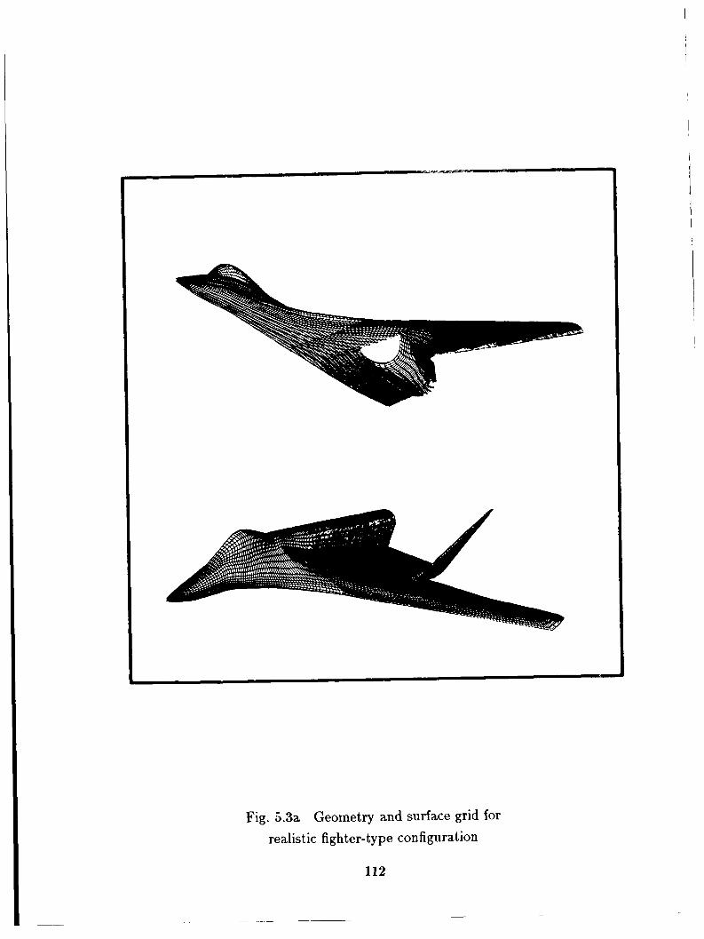
Fig. 5.3a Geometry and surface grid for realistic fighter-type configuration

112

I

W 2 3 a W F 2 W 0 a W e e 3

I I I I

I I I I

d 3 ,

' 0 el d 0 0 0 0 d (v

I I

Fig. 5.3b Surface pressure distribution along upper symmetry plane

0 0 d

3 3 n

c X .II U

3 3 U

> > m

113

1 I I I

I

P 0

Fig. 5 . 3 ~ Surface pressure distribution along lower symmetry plane

0 0 d

0 0 M

n c X .I 21

3 3 N

3 3 I

I

114

Z

Fig. 5.3d Pressure contours at x = 550in.

115

I I I A FULL POTENTIAL A

-EULER

X = 550 IN. 0.2 -

cP

-0.2 e-””-----42 0 100 200

Fig. 5.3e Circumferential pressure distribution

116

250

170

90

Y

10

-70

-1 50 I I I I

z 0 80 160 240 320 400

Fig. 5.3f Pressure contours at x = 688 in.

117

0 0 (9

0 0 (Y

0 0 P

3

Fig. 5.3g Circumferential pressure distribution

118

5.7.3 Space Shuttle Orbiter

Figs. 5.4a-5.4g give the geometry, gridding and corresponding flow-field solutions for an isolated Space Shuttle Orbiter flying at M, = 1.4,cr = Oo. The EMTAC code is applied to compute the flow field about the entire orbiter, from nose to tail. Multiple (uni- or bi-directional sweeps are used in the nose region to capture the detached bow shock and the subsonic region behind it. After this subsonic region transitions by expansion, over the shoulder region of the nose, into a supersonic flow-field, a simple forward-marching technique is employed. Multiple relaxation sweeps are also used in the canopy and OHMS pod regions to compute the locally subsonic regions.

The surface pressure distribution along the leeward plane of symmetry in the nose region is presented in Fig. 5.4b. At x = 170in., which is the beginning of the canopy, the pressure increases rapidly from Cp = 0.3 to w 1.0. An embedded subsonic pocket is formed in the canopy region and required three relaxation marching sweeps to develop the solution. The results show that the present prediction is in excellent agreement with data. Pressure contours on the upper symmetry plane and on the marching plane cross-sectional views are shown in Fig. 5 . 4 ~ . The shock and expansion waves induced by the canopy can be clearly seen in this figure.

Fig. 5.4d shows the details of the orbiter geometry in the OMS pod region as modeled in this study. A detached OMS pod shock and a large subsonic pocket are formed in this region. Since the subsonic pocket is big and the Mach number is almost zero near the root of the OMS pod, a total of 30 relaxation marching sweeps (forward only) are required to give a good, converged result. Fig. 5.4e presents the pressure and Mach number contours as obtained in this region. The cross-sectional pressure contours at x = 1080in. and x = 1125in. are given in Fig. 5.4f. The OMS pod shock is formed around x = 1050in., then grows and finally hits the upper wing surface at x rn 1095 in.. The chordwise pressure distributions on the upper surface of the wing at several span stations are compared with experimental data in Fig. 5.4g. It is seen that the present ca!ciilat,ion agrees with the experimental data very well over the entire upper surface including in the region where the OMS pod shock interacts with the wing surface.

5.8 REMARKS

A new computational procedure has been devised to solve the Euler equations for three-dimensional supersonic inviscid flows with subsonic pockets. The method is akin to a simple marching procedure in portions of the flow field where the component of velocity normal to the local marching plane is supersonic. When this local velocity is subsonic

119

x = 725" x = 925" x = 1200"

Fig. 5.4a Shuttle Orbiter configuration and sample grids

120

I

n

C

X .I V

0

0 0 m

3 3 N

n C

X .I U

3 3 r

3

Fig. 5.4b Surface pressure distribution along upper symmetry plane

121

v)

3 0 I- 2 0 0 w 3 v) v) w

a

a

a n

t I t

v) a 3 0 k 2 0 0 W a 3

I I I I i I

0 0 0 r m h

I cy m 0 0 r h cy

I I >

>

0 <o m

0 cy *

0 00N cy

0 * r

0

0

1

> Fig. 5 . 4 ~ Canopy region pressure contours for

z - y and z - y sectional cuts

122

I

Fig. 5.4d Computational surface geometry of Orbiter at OMS pod region

123

cn U 3 0 I= z 0 0 U w :

2

3 z I 0

I I I I

I

I I I I

* 0

Fig. 5.4e Pressure and Mach number contours at OMS pod region: z - y section

124

0 i

v)

3 0 + z 0 0 W

3 v) v) W

a

a

a e

v) a 3 0 c 2 0 0 W a 3 v) v) W a e

C C 7

0

I I I I ’\, Qo , o

I I > Fig. 5.4f Pressure contours at OMS pod region:

z - y section

N

N

125

h cy t 0 I1 F

J 2 0 -

t c3 ua I1 F

0

c3 0 h cy r* 00 00 h CD b 00 ua 0 0 0 0 I1 i1 i1 i1

F F t= F

Lllll t c y o q t 0 0 0 0

P

0 0 Ir) r=

0 0 m r

0 0 N I=

xo 0 0 r r

0 0 0 F

0 0 Q)

Fig. 5.4g Orbiter upper surface pressure distribution

126

(in subsonic pockets for example), a relaxation approach is used. The marching and relaxation strategies are both but variations of a unified approach to the development of finite difference methods for this class of problems. This approach is based on a planar Gauss-Seidel procedure coupled with approximate factorization in the plane. Being an expository effort, detailed formulae are presented to aid the reader who would like to program the method independently.

It is of interest to note the following observations: The method presented is not only applicable to supersonic flows with subsonic pockets, but is also applicable to all compressible inviscid flow regimes including entirely subsonic, transonic (subsonic flow with supersonic pockets), and entirely supersonic flows. By iterating in just one marching plane, a computer program based on the method presented can be used to also solve problems that are two-dimensional or that can be reduced to two dimensions. Conical flows are examples of the latter. The same computer program can also be used to solve three-dimensional (and two-dimensional) unsteady flows. Thus, the unified approach taken is really greater in scope and applicability than what the title of this section might suggest. Of course, the method is eminently suitable for the case of supersonic flows with subsonic pockets.

The use of TVD discretizations results in a highly reliable method with no artificial parameters such as coefficients of numerical smoothing to be provided by the user. Spurious oscillations and expansion shocks are also eliminated.

The relaxation approach used can also be used to solve the Navier-Staokes equation^'^. By following the unified methodology used to derive the present algorithm for the Euler equations, a unified scheme can also be derived for the Navier-Stokes equations. Parab- olized forms of the Navier-Stokes equations may be solved in regions where there is little upstream propagating influence upon the boundary layer and when the flow external to the boundary layer is supersonic. In regions of separation, etc. where there is an appre- ciable effect of the downstream upon the upstream flow, and/or where the external flow is subsonic, the relaxation approach may be used. Such methods can provide superior replacements to current Parabolized Navier-Stokes solvers.

127

Section 6.0

CONCLUDING REMARKS

This report has dealt with many aspects of upwind schemes for hyperbolic systems i 4

of conservation laws in general and for the Euler equations in particular. The report began by discussing various formulations of upwind schemes. An operational unification of several underlying flux-difference-split and flux-split approaches was presented. The design of higher-order upwind schemes using the Total Variation Diminishing formulation was described along with a discussion of the preprocessing and postprocessing approaches. The formulation of the method for arbitrarily shaped control volumes was outlined. Many useful properties of TVD upwind formulations were pointed out. Relaxation methods for unfactored implicit formulations of upwind schemes were covered in some detail. The postprocessing approach was used to develop the details of the discretization procedure in two and three dimensions in Cartesian and general curvilinear coordinate systems. All the features of TVD upwind schemes discussed above have been used to develop a computer program to solve the Euler equations efficiently for three-dimensional supersonic flows with subsonic pockets. The algorithmic framework for this code has been presented in some detail.

,

Higher-order accurate upwind schemes based on TVD formulations are now in use in many industrial and government facilities. They come in many forms, some of which have been covered in this report. This signifies the attainment of a certain level of maturity in this area of research and development. Much remains to be done however. It is not yet clear whether the preprocessing approach is more advantageous than the postprocessing approach or vice-versa. Both approaches seem to be effective and useful and therefore this question may not be that important. This report included a description of one approach to the construction of upwind schemes for triangular control areas. This approach has not been fully exploited yet.

This author is convinced that the underlying formulations described in this report will be of substantial use for many years to come. However, there are already some new developments which promise to dramatically improve the state of the art. TVD formulations of upwind schemes are inherently limited to second-order global accuracy for unsteady problems and possible third-order accuracy for steady-state problems. Better formulations are now possible which have no such restrictions but which still result in essentially oscillation-free solutions for any order of accuracy.

128

Seetion 7.0 REFERENCES

t

t

i

t

[I] S. Chakravarthy and S. Osher, “Numerical Experiments with the &her Upwind Scheme for the Euler Equations,” AIAA Joztmaf, Volume 21, Number 9, September 1983, pp. 1241-1248.

[2] S. R. Chakravarthy and S. Osher, “High Resolution Applications of the Osher Upwind Scheme for the Euler Equations,” AIAA Paper 83-1943, Proceedings of the AEAA Sixth Computational Fluid Dynamics Conference, Dmvers, Massachusetts, July 1983, pp. 363-372.

[3] S. R. Chakravarthy, “Properties and Applications of Modern Upwind Difference Schemes for Hyperbolic Systems of Conservation Laws,” in Advances in Comp~rtafional Methods for Boundary and Interior Layers, Lecture Notes of an International Short Course held in association with BAIL 111 Conference, 18-19 June 1984, Trinity College, Dublin, Ireland; Ed. J.J.H. Miller; h o l e Press, 1984.

(41 S. R. Chakravarthy and S. Osher, “Computing with High-Resolution Upwind Schemes for Hyperbolic Equations,” Large-Scale Computations in Fluid Mechanics, Volume 22- Pzrt 1, Lectures in Applied Mathematics, American Mathematical Society, 1985, pp. 57-86.

[5] S. R. Chakravarthy, “Relaxation Methods €or Unfactored Implicit Upwind Schemes,” AIAA Paper 84-0165, 1984, January 1984.

[6] S. R. Chakravarthy and S. Osher, “A New Class of High Accuracy TVD Schemes for Hyperbolic Conservation Laws,” AIAA Paper 85-0363, January 1985.

[7] S. R. Chakravarthy and K-Y. Szema, “An Euler Solver for Supersonic Flows with Subsonic Pockets,” AIAA Paper No. 85-1703, July 1985.

[8] K. Y. Szema, S. R. Chakravarthy, V. Shankar, and J . Byerly, “Comparison of Euler and h i 1 Potentiai Marching Techniques €or Flows over Complex Configurations,” AIAA Paper No. 86-0244, January 1986.

(91 A. Harten, “High Resolution Schemes for Hyperbolic Conservation Laws,” Journal of Computational Physics, Vol. 49, 1983, pp. 357-393.

129

[IO] S. Osher and S. R. Chakravarthy, “High Resolution Schemes and the Entropy Condi- tion,” NASA CR-172218, ICASE, September 1983.

[I l l P. K. Sweby, “High Resolution Schemes Using Flux Limiters for Hyperbolic Conser- vation Laws,” SIAM Journal on Numerical Analysis, Vol. 21, No. 5, October 1984, pp. 995-1011.

[I21 S. Osher and S. R. Chakravarthy, “Very High Order Accurate TVD Schemes Ap- proximating Hyperbolic Conservation Laws,” ICASE Report No. 84-44, 1984, NASA Langley Research Center.

1131 A. Harten, “On a Class of High Resolution Total-Variation-Stable Finite-Difference Schemes,” SIAM Journal on Numerical Analysis, Vol. 21, No. 1, February 1984, pp. 1- 23.

I141 J. B. Goodman and R. J. Leveque, “On the Accuracy of Stable Schemes for Two Dimensional Conservation Laws,” Mathematics of Computation, Vol. 45, 1985, pp. 15- 21.

(151 S. Osher and S. R. Chakravarthy, “High Resolution Schemes and the Entropy Condi- tion,” SIAM Journal on Numerical Analysis, Vol. 21, No. 5, October 1984, pp. 955-984.

[ 16) S. Osher, “Convergence of Generalized MUSCL Schemes,” NASA Langley Research Center Contractor Report 172306, 1984.

[17] S. R. Chakravarthy, K-Y. Szema, U. C. Goldberg, J . J. Gorski, and S. Osher, “Applica- tion of a New Class of High Accuracy TVD Schemes.to the Navier-Stokes Equations,” AIAA Paper No. 85-0165, January 1985.

[18] J . J . Gorski, S. R. Chakravarthy, and U. C. Goldberg, “High Accuracy TVD Schemes for the k-e Equations of Turbulence,” AIAA Paper No. 85-1665, July 1985.

[19] S. K. Godunov, “A Finite Difference Method for the Numerical Computation of Dis- continuous Solutions of the Equations of Fluid Dynamics,” Matematic‘eskif Sbornik, Vol. 47, 1959, pp. 271-290, also Cornel1 Aeronautical Laboratory translation.

[20] P. L. Roe, “Approximate Riemann Solvers, Parameter Vectors, and Difference Schemes,” Journal of Computational Physics, Vol. 43, 1981, pp. 357-372.

[21] S. Osher, “Numerical Solution of Singular Perturbation Problems and Hyperbolic Systems of Conservation Laws,” Analytical and Numerical Approaches to Asymptotic

130

Problems in Analysis, North Holland Mathematical Studies No. 47, Edited hy S. Ax- elsson, L. S. Frank, and A. van der Sluis, 1981, pp. 179-205.

[a21 J. L. Steger and R. F. Warming, “Flux Vector Splitting of the Inviscid Gasdynamic Equations with Application to Finite Difference Methods,” NASA TM-78605, July 1979.

[23] S. Osher, “Riemann Solvers, the Entropy Condition, and Difference Approximations,” SIAM Journal on Numerical Analysis, Vol. 21, No. 3, 1984, pp. 217-235.

[24] P. Colella, “A Direct Eulerian MUSCL Scheme for Gas Dynamics,” Lawrence Berkeley Laboratory Report No. LBL-14104, 1982.

[25] P. Colella and P. R. Woodward, “The Piecewise-Parabolic Method (PPM) for Gas- dynamical Simulations,” Lawrence Berkeley Laboratory Report No. 14661, July 1982.

[26] H. C. Yee, R. F. Warming, and A. Harten, “Implicit Total Variation Diminishing (TVD) Schemes for Steady State Calculations,” AIAA Paper 83-1902, Proceedings of the AIAA Sixth Computational Fluid Dynamics Conference, Danvers, Massachusetts, July 1983, pp. 110-127.

[27] W. A. Mulder and B. van Leer, “Implicit Upwind Computations for the Euler Equa- tions,” AIAA Paper 83-1930, Proceedings of the AIAA Sixth Computational Fluid Dynamics Conference, Danvers, Massachusetts, July 1983, pp. 303-310.

[28] B. van Leer, “Towards the Ultimate Conservative Difference Scheme IV. A New Ap- proach to Numerical Convection,” Journal of Computational Physics, Vol. 23, 1977, pp. 276-299.

[29] B. van Leer, “On the Relation Between the Upwind Differencing Schemes of Godunov, Engquist-Osher, and Roe,” SIAM Journal on Scientific and Statistical Computing, Vol. 5, 1984, pp. 1-20.

[30] B. van Leer, “Towards the Ultimate Conservative Difference Scheme 111. Upstream Centered Finite-Difference Schemes for Ideal Compressible Flow ,” Journal of Compu- tational Physics, Vol. 23, 1977, pp. 263-275.

[31] R. M. Beam and R. F. Warming, “An Implicit Finite-Difference Algorithm for Hy- perbolic Systems in Conservation-Law Form,” Journal of Computational Physics, ” Volume 22, 1976, pp. 87-110.

131

[32] €I. McDonald and W. R. Briley, “Three-Dimensional Supersonic Flow of a Viscous or Inviscid F~ow,” Journal of Computational Physics, Volume 19, 1975, pp. 150-178.

I [33] P. G. Buning and J. L. Steger, “Solution of the Two-Dimensional Euler Equations with Generalized Coordinate Transformation using Flux Vector Splitting,” AIAA Paper 82-0971, June 1982.

[34] S. R. Chakravarthy, D. A. Anderson, and M. D. Salas, “The Split-Coefficient Matrix Method for Hyperbolic Systems of Gasdynamic Equations,” AIAA Paper 80-0268, January 1980. i

1351 S. R. Chakravarthy, “The Split-Coefficient Matrix Method for Hyperbolic Systems of Gasdynamic Equations,” Ph. D. Thesis, Department of Aerospace Engineering, Iowa State University, Ames, Iowa, November 1979.

I

[36] P. L. Roe and M. J . Baines, “Algorithms for Advection and Shock Problems,” Pro- ceedings of the 4th GAMM Conference on Numerical Methods in Fluid Mechanics, 1982, Ed. €I. Viviand.

[37] V. Shankar, “Implicit Treatment of the Unsteady Full Potential Equation in Conser- vation Form,” AIAA Paper No. 84-0262, January 1984.

[38] N. L. Sankar, “A Multigrid Strongly Implicit Procedure for Two-Dimensional Tran- sonic Potential Flow Problems,” AIAA Paper 82-0931, June 1982.

[39] A. N. Lyubimov and V. V. Rusanov, “Gas Flows Past Blunt Bodies,” Part 11: Tables of Gasdynamic Functions, NASA TT F-715, Feb. 1973.

[40] V. Shankar, K. Y. Szema, and S. Osher, “A Conservative Type-Dependent Full Poten- tial Method for the Treatment of Supersonic Flow with Imbedded Subsonic Region,” AIAA Paper No. 83-1887, July 1983.

[41] K. Y. Szema and V. Shankar, “Nonlinear Computation of Wing-Body-Vertical Tail- Wake Flows at Low Supersonic Speed,” AIAA Paper No. 84-0427, January 1984.

[42] K. Y. Szema, W. L. Riba, V. Shankar, and J. J. Gorski, “Full Potential Treatment of Flows Over 3-D Geometries Including Multi-body Configurations,” AIAA Paper No. 85-0272, January 1985.

[43] S. R. Chakravarthy and D. K. Ota, “Numerical Issues in Computing Inviscid Super- sonic Flow Over Conical Delta Wings,” AIAA Paper 86-0440, January 1986.

132

I

[44] S. R. Chakravart hy, “Euler Quations- Implicit Schemes and Boundary Conditions,”

I A l A A Journal, Volume 21, Number 5, May 1983, pp. 699-706.

[45] J. C. Townsend, D. T . Howell, I. K. Collins, and C. Hayes, “Surface Pressure Data on a Series of Analytic Forebodies at Mach Numbers from 1.70 to 4.50 and Combined Angles of Attack and Sideslip,” NASA TM-80062, June 1979.

I

133

Standard Bibliographic Page

I. Report No. NASA CR-4043

2. Government Accession No. 3. Recipient's Catalog No.

16. Abstract T h i s r e p o r t descr ibes many a l g o r i t h m i c and computat ional aspects o f upwind schemes and t h e i r second-order accura te f o r m u l a t i o n s based on T o t a l - V a r i a t i o n - D i m i n i s h i n g (TVD) approaches. An o p e r a t i o n a l u n i f i c a t i o n o f t h e u n d e r l y i n g f i r s t - o r d e r scheme i s f i r s t presented encompassing Godunov's, Roe's, Osher 's, and S p l i t - F l u x methods. For h i g h e r o r d e r vers ions , t h e preprocess ing and pos tprocess ing approaches t o c o n s t r u c t i n g TVD d i s c r e t i z a t i o n s a r e considered. TVD f o r m u l a t i o n s can be used t o c o n s t r u c t r e l a x a t i o n methods for un fac tored i m p l i c i t upwind schemes which i n t u r n can be e x p l o i t e d t o c o n s t r u c t space-marching procedures f o r even t h e unsteady Euler equat ions. A major p a r t o f t h e r e p o r t descr ibes t ime- and space- mar'ching procedures f o r s o l v i n g the E u l e r equat ions i n 2-D, 3 -D , Car tes ian , and c u r v i l i n e a r coord ina tes . Along w i t h many i l l u s t r a t i v e examples, severa l r e s u l t s o f e f f i c i e n t computat ions on 3-D supersonic f l o w s w i t h subsonic pockets a r e presented.

I. Title and Subtitle

Equa t ions Development o f Upwind Schemes f o r t h e E u l e r

5. Report Date January 1987

6. Performing Organization Code

r. Author(s)

Sukumar R. Chakravar thy

Rockwell I n t e r n a t i o n a l Science Center P.O. Box 1085 Thousand Oaks, C a l i f o r n i a 91360

B . Performing Organization Name and Address

1

12. Sponsoring Agency Name and Address

N a t i o n a l Aeronaut ics and Space A d m i n i s t r a t i o n Washington, DC 20546

8. Performing Organization Report No. sc5388.40FR

10. Work Unit No.

11. Contract or Grant No. NAS1-17492

13. Type of Report and Period Covered Contractor Report Oct. 12, 1983-Feb. 27, 1986

14. Sponsoring Agency Code

17. Key Words (Suggested by Authors(s))

Upwind Schemes, T o t a l - V a r i a t i o n - D i m i n i s h i n g (TVD) Schemes, Second-Order Accuracy Supersonic Flows w i t h Subsonic Pockets

18. Distribution Statement

U n c l a s s i f i e d - U n l i m i t e d

S u b j e c t Category 02

19. Security Classif.(of this report) 20. Security Classif.(of !hi- page) 21. No. of Pages U n c l a s s i f i e d U n c l a s s i f i e d 138

22. Price

A 0 7

for the Euler Equations - ntrs.nasa.gov · for the Euler Equations ... 2.8 Diagonal Dominance in...

Documents

Transcript of for the Euler Equations - ntrs.nasa.gov · for the Euler Equations ... 2.8 Diagonal Dominance in...