for Outline - World Meteorological Organization fileNWP skill with FIM vs. GFS 4 ... Brown, Stan...
4
10/31/2014 1 Stan Benjamin, Shan Sun, Rainer Bleck, Georg Grell, John Brown, George Kiladis, Randall Dole, Judith Perlwitz NOAA Earth System Research Laboratory, Boulder CO USA Experiments with the FIM global model for blocking and related processes for sub‐seasonal to medium‐range forecast duration 1 WWOSC – 19 Aug 2014 March 2012 N. American block Θ on PV2 (dyn tropopause) 10km FIM – 21-31 Mar 2014 Outline 1. Problem: stationary wave events 2. Refinements to FIM atmos/ocean/chem global coupled model to improve both NWP and seasonal prediction. Co‐development for both applications. 3. NWP skill with FIM vs. GFS 4. Preliminary experiments a. March 2014 troposphere/stratosphere case b. MJO experiments –2 month duration c. 1‐year experiment results for stationary waves with different resolution/waves 5. Plans for stationary‐wave process experiments and FIM applications within larger NOAA model development. 2 1 – stat wave prob 2 – FIM desc 3 – NWP skill 4 – experiments 5 – plans Blocking frequency as a function of global model resolution Jung et al., 2012, J. Climate: High-res ECMWF experiments for Project ATHENA T511 necessary T511 topo necessary AMIP Tibaldi-Molteni Index 1 – stat wave prob 2 – FIM desc 3 – NWP skill 4 – experiments 5 – plans Processes related to blocking onset, cessation, prolongation• Extratropical wave interaction • MJO life cycle • Other tropical procs/ENSO • Tropical storms and their extratropical transitions • Sudden stratospheric warming events • Snow cover anomalies • Soil moisture anomalies Initial valuedata assim High‐res Δx Coupled ocean Stochastic physics PV cons. numerics Chem/aerosol Soil/snow LSMaccuracy ✔ ✔ ✔ ✔ ✔ ✔ ✔ ✔ ✔ ✔ ✔ ✔ ✔ ✔ ✔ ✔ ✔ ✔ ✔ ✔ ✔ ✔ ✔ ✔ ✔ ✔ ✔ ✔ ✔ ✔ ✔ ✔ Model component sensitivity NOAA/Navy/others Earth System Prediction Capability ESPC focus target: improved 1-6 month fcst of blocking 4 Flow-following- finite-volume Icosahedral Model FIM X-section location Temp at lowest level http://fim.noaa.gov Key developers ESRL - Rainer Bleck, Shan Sun, Ning Wang, Jian-Wen Bao, John Brown, Stan Benjamin, Georg Grell, (Jin Lee, Sandy MacDonald) 1 – stat wave prob 2 – FIM desc 3 – NWP skill 4 – experiments 5 – plans FIM design – vertical coordinate Hybrid (sigma/ isentropic) vertical coordinate • Improved conservation using quasi-material surfaces, reduced vertical dispersion. Improved transport by reducing numerical dispersion from vertical cross- coordinate transport, improved stratospheric/tropospheric exchange. • Used in NCEP Rapid Update Cycle (RUC) model • Used in HYCOM ocean model Installed as generalized “s” vertical coordinate - can be replaced with sigma-p or other coordinates. 6
Transcript of for Outline - World Meteorological Organization fileNWP skill with FIM vs. GFS 4 ... Brown, Stan...

10/31/2014
1
Stan Benjamin, Shan Sun, Rainer Bleck, Georg Grell, John Brown, George Kiladis, Randall Dole, Judith PerlwitzNOAA Earth System Research Laboratory, Boulder CO USA
Experiments with the FIM global model for blocking and related processes for sub‐seasonal to
medium‐range forecast duration
1
WWOSC – 19 Aug 2014March 2012 N. American block
Θ on PV2 (dyn tropopause)10km FIM – 21-31 Mar 2014
Outline1. Problem: stationary wave events
2. Refinements to FIM atmos/ocean/chem global coupled model to improve both NWP and seasonal prediction. Co‐development for both applications.
3. NWP skill with FIM vs. GFS
4. Preliminary experimentsa. March 2014 troposphere/stratosphere case
b. MJO experiments – 2 month duration
c. 1‐year experiment results for stationary waves with different resolution/waves
5. Plans for stationary‐wave process experiments and FIM applications within larger NOAA model development.
2
1 – stat wave prob2 – FIM desc3 – NWP skill4 – experiments5 – plans
Blocking frequency as a function of global model resolutionJung et al., 2012, J. Climate: High-res ECMWF experiments for Project ATHENA
T511 necessary
T511 toponecessary
AMIP
Tibaldi-Molteni Index
3
1 – stat wave prob2 – FIM desc3 – NWP skill4 – experiments5 – plans
Processes related to blocking onset, cessation, prolongation
• Extratropical wave interaction
• MJO life cycle
• Other tropical procs/ENSO
• Tropical storms and their extratropical transitions
• Sudden stratospheric warming events
• Snow cover anomalies
• Soil moisture anomalies
Initialvalue –
data assim
High‐res
Δx
Coupledocean
Stochastic
physics
PVcons.
numerics
Chem
/aerosol
Soil/snowLSM
accuracy
✔ ✔ ✔ ✔
✔ ✔ ✔ ✔ ✔ ✔
✔ ✔ ✔ ✔ ✔
✔ ✔ ✔ ✔ ✔ ✔ ✔
✔ ✔ ✔
✔ ✔ ✔
✔ ✔ ✔ ✔
Model component sensitivity NOAA/Navy/others Earth System Prediction CapabilityESPC focus target: improved 1-6 month fcst of blocking
4
Flow-following-finite-volume
Icosahedral Model FIM
X-section location
Temp at lowest level
http://fim.noaa.gov
Key developers
ESRL - Rainer Bleck, Shan Sun, Ning Wang, Jian-Wen Bao, John Brown, Stan Benjamin, Georg Grell, (Jin Lee, Sandy MacDonald)
5
1 – stat wave prob2 – FIM desc3 – NWP skill4 – experiments5 – plans
FIM design – vertical coordinateHybrid (sigma/ isentropic) vertical coordinate • Improved conservation using quasi-material surfaces, reduced vertical dispersion.
Improved transport by reducing numerical dispersion from vertical cross-coordinate transport, improved stratospheric/tropospheric exchange.
• Used in NCEP Rapid Update Cycle (RUC) model
• Used in HYCOM ocean model
Installed as
generalized “s” vertical
coordinate- can be replaced with
sigma-p or other coordinates.
6
10/31/2014
2
7
Mean cross-coordinate transport – 24h FIM quasi-lagrangian hybrid θσ coord (no-physics)sigma coordinate (no physics)
Stratosphere
Uppertroposphere
Lowertroposphere
1 – stat wave prob2 – FIM desc3 – NWP skill4 – experiments5 – plans
Reduced cross-coord transport (numerical diffusion) with QL θσ vert coord
Mean abs
FIM numerical atmospheric model•Horizontal grid
• Icosahedral, ∆x=240km/120km / 60km/30km/15km/10km•Vertical grid
• ptop = 0.5 hPa, θtop ~2200K• Generalized vertical coordinate
• Hybrid θ-σ option (64L, 38L, 21L options currently)• GFS-like σ-p option (64 levels)
•Physics• GFS physics suite (May 2011 version, May 2013 McICA
radiation), options for Grell-Freitas cumulus, WRF opts•Coupled model extensions
• Chem – WRF-chem/GOCART• Ocean – icosahedral HYCOM (no coupler), tri-polar
HYCOM (with coupler)8
iHYCOM vertical section. Heavy black lines: coordinate surfaces. Shaded contours: potential density (
FIM vertical section. Heavy black lines: coordinate surfaces. Colored field: pot.temperature (K). Shaded contours: potential vorticity.
10
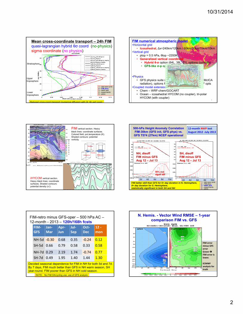
500-hPa Height Anomaly CorrelationFIM-30km (GFS init, GFS phys) vs.
GFS T574 (27km) NCEP operational
SH, dieoffJun12 – May13
12‐month NWP testAugust 2012 ‐July 2013
NH, dieoffFIM minus GFSAug 12 – Jul 13
SH, dieoffFIM minus GFSAug 12 – Jul 13
95% stat signif diff
2d 4d 6d 8d 10d 2d 4d 6d 8d 10dFIM better skill than GFS for 5+ day duration in N. Hemisphere, 4+ day duration for S. Hemisphere, statistically significant in both SH and NH
1 – stat wave prob2 – FIM desc3 – NWP skill4 – experiments5 – plans
FIM‐GFS
Jan‐Mar
Apr‐Jun
Jul‐Sep
Oct‐Dec
12 ‐mon
NH‐5d ‐0.30 0.68 0.35 ‐0.24 0.12
SH‐5d 0.66 0.79 0.58 0.33 0.58
NH‐7d 0.29 2.19 1.74 ‐0.74 0.77
SH‐7d 0.49 1.95 1.40 1.44 1.30
FIM-retro minus GFS-oper – 500 hPa AC –12-month - 2013 – 120h/168h fcsts
Decided seasonal dependence for FIM in NH for both 5d and 7d.By 7 days, FIM much better than GFS in NH warm season, SH year-round. FIM poorer than GFS in NH cold season.
NOTE: No FIM DA/cycling use, use of GFS analysis
N. Hemis. - Vector Wind RMSE – 1-year comparison FIM vs. GFS
FIM error minus GFS errorGreen FIM error is lower.
ECMWF analysis for truth

10/31/2014
3
13
12h 24h 36h 48h 72h 96h 120h
• FIM usually better than GFS for hurricane track forecasts over last 3 years for 72h‐120h (3‐5 day) forecasts, ECMWF better than FIM or GFS
• Both FIM and GFS used the same hybrid initial conditions, same physics.
3‐year (2011‐2013) hurricane track error results –% forecast error (FE) improvement over HFIP baseline. Larger = better.
Atlantic E. Pacific
12h 24h 36h 48h 72h 96h 120h
1 – stat wave pro2 – FIM desc3 – NWP skill4 – experiments5 – plans
PV on 590K surface10-day forecast init 00z 21 Mar 2014FIM 10km θ-σ modelHourly output
250hPa v-compHövmuller diag
1 – stat wave prob2 – FIM desc3 – NWP skill4 – experiments5 – plans
θ‐σ (solid) vs. σ‐p (dashed)
Mean 10hPa zonal wind @60N – Mar2014 – obs vs. FIM fcsts
21 Mar runs capture breakdown, but only θ‐σ version for 15 Mar 2‐week run
Stratospheric vortex breakdownPV on 600K sfc valid 00 UTC 28 Mar 2014
FIM θ‐σ (adaptive) vs. FIM σ‐p (fixed) vertical coord 16
Stratospheric vortex breakdownPV on 600K sfc valid 00 UTC 28 Mar 2014
Obs28 Mar
12 Mar init ‐ FIM 15 Mar init ‐ FIM
18 Mar init ‐ FIM 21 Mar init ‐ FIM
FIM fcsts valid 00 UTC 28 Mar 2014
1 – stat wave prob2 – FIM desc3 – NWP skill4 – experiments5 – plans
Cloud - 10-day forecast init 00z 21 Mar 2014FIM θ-σ model – 10km 64L
Visualization – Jebb Stewart, Steve Albers – ESRL/GSD
250hPa v-compHövmuller diag
18
Feb-March 2012 – outgoing LW rad (OLR) Preliminary MJO experiments with FIM (AMIP) 2-mo runs
Observed OLR – HIRS1° data from NCDC
Courtesy – George Kiladis, NOAA/ESRL/PSD
Init 1 Feb30km FIM-theta
Init 2 Feb
15km FIM-theta
With 30km land/water
Next experiments in progress or near future• 15km FIM with 15km land-water for improved Maritime Continent detail• 15km and 30km with Grell-Freitas cu parm• CMIP vs. AMIP• All above with init every 2 days thru 15 Mar
60km FIM
30km FIM-sig
1 – stat wave prob2 – FIM desc3 – NWP skill4 – experiments5 – plans
10/31/2014
4
19
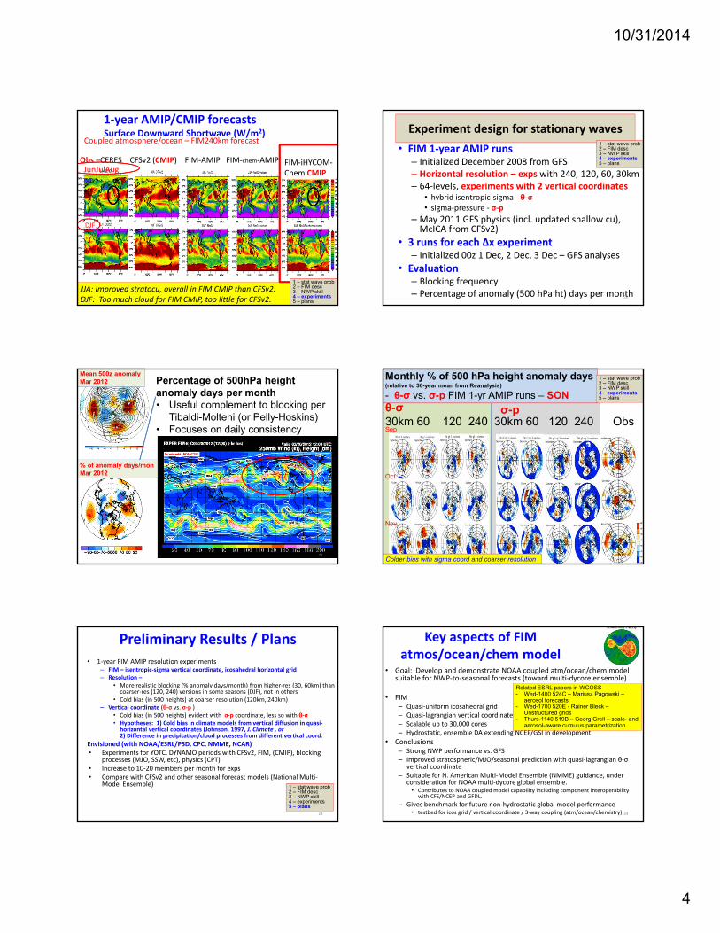
1‐year AMIP/CMIP forecastsSurface Downward Shortwave (W/m2)
Coupled atmosphere/ocean – FIM240km forecast
DJF
Obs –CERES CFSv2 (CMIP) FIM‐AMIP FIM‐chem‐AMIPJunJulAug
JJA: Improved stratocu, overall in FIM CMIP than CFSv2. DJF: Too much cloud for FIM CMIP, too little for CFSv2.
FIM‐iHYCOM‐Chem CMIP
1 – stat wave prob2 – FIM desc3 – NWP skill4 – experiments5 – plans
Experiment design for stationary waves
• FIM 1‐year AMIP runs– Initialized December 2008 from GFS– Horizontal resolution – exps with 240, 120, 60, 30km– 64‐levels, experiments with 2 vertical coordinates
• hybrid isentropic‐sigma ‐ θ‐σ• sigma‐pressure ‐ σ‐p
– May 2011 GFS physics (incl. updated shallow cu), McICA from CFSv2)
• 3 runs for each Δx experiment– Initialized 00z 1 Dec, 2 Dec, 3 Dec – GFS analyses
• Evaluation– Blocking frequency– Percentage of anomaly (500 hPa ht) days per month20
1 – stat wave prob2 – FIM desc3 – NWP skill4 – experiments5 – plans
21
Percentage of 500hPa height anomaly days per month• Useful complement to blocking per
Tibaldi-Molteni (or Pelly-Hoskins)• Focuses on daily consistency
% of anomaly days/monMar 2012
Mean 500z anomalyMar 2012
θ-σ30km 60 120 240 30km 60 120 240 Obs
Monthly % of 500 hPa height anomaly days(relative to 30-year mean from Reanalysis)
- θ-σ vs. σ-p FIM 1-yr AMIP runs – SON
σ-p
Sep
Oct
Nov
22
1 – stat wave prob2 – FIM desc3 – NWP skill4 – experiments5 – plans
Colder bias with sigma coord and coarser resolution
Preliminary Results / Plans• 1‐year FIM AMIP resolution experiments
– FIM – isentropic‐sigma vertical coordinate, icosahedral horizontal grid– Resolution –
• More realistic blocking (% anomaly days/month) from higher‐res (30, 60km) than coarser‐res (120, 240) versions in some seasons (DJF), not in others
• Cold bias (in 500 heights) at coarser resolution (120km, 240km)– Vertical coordinate (θ‐σ vs. σ‐p )
• Cold bias (in 500 heights) evident with σ‐p coordinate, less so with θ‐σ• Hypotheses: 1) Cold bias in climate models from vertical diffusion in quasi‐horizontal vertical coordinates (Johnson, 1997, J. Climate , or 2) Difference in precipitation/cloud processes from different vertical coord.
Envisioned (with NOAA/ESRL/PSD, CPC, NMME, NCAR)• Experiments for YOTC, DYNAMO periods with CFSv2, FIM, (CMIP), blocking
processes (MJO, SSW, etc), physics (CPT)• Increase to 10‐20 members per month for exps• Compare with CFSv2 and other seasonal forecast models (National Multi‐
Model Ensemble)
23
1 – stat wave prob2 – FIM desc3 – NWP skill4 – experiments5 – plans
Key aspects of FIM atmos/ocean/chem model
• Goal: Develop and demonstrate NOAA coupled atm/ocean/chem model suitable for NWP‐to‐seasonal forecasts (toward multi‐dycore ensemble)
• FIM– Quasi‐uniform icosahedral grid– Quasi‐lagrangian vertical coordinate– Scalable up to 30,000 cores – Hydrostatic, ensemble DA extending NCEP/GSI in development
• Conclusions– Strong NWP performance vs. GFS– Improved stratospheric/MJO/seasonal prediction with quasi‐lagrangian θ‐σ
vertical coordinate– Suitable for N. American Multi‐Model Ensemble (NMME) guidance, under
consideration for NOAA multi‐dycore global ensemble.• Contributes to NOAA coupled model capability including component interoperability
with CFS/NCEP and GFDL.
– Gives benchmark for future non‐hydrostatic global model performance• testbed for icos grid / vertical coordinate / 3‐way coupling (atm/ocean/chemistry) 24
Related ESRL papers in WCOSS- Wed-1400 524C – Mariusz Pagowski –
aerosol forecasts- Wed-1700 520E - Rainer Bleck –
Unstructured grids- Thurs-1140 519B – Georg Grell – scale- and
aerosol-aware cumulus parametrization