For DOT/VOLPE nd - National Highway Traffic Safety ... linear proprieties such as Mass, Aerodynamic...

Engine Parametric Study+/- 10kW range with a step of 1kW

“This presentation does not contain any proprietary or confidential information”

Ayman Moawad, Aymeric RousseauArgonne National Laboratory

For DOT/VOLPEJun 02nd , 2015

Results Summary

2

For conventional vehicles, increasing/decreasing the engine power by 10kW leads to an increase/decrease in fuel consumption by a range of:

• 3.3% and 3.4% for Eng5a• 3.1% and 3.3% for Eng5b• 3.0% and 3.1% for Eng5c• 2.7% and 3.0% for Eng6a• 2.5% and 2.9% for Eng6b• 2.5% and 2.9% for Eng7a• 2.4% and 2.8% for Eng7b• 1.8% and 2.2% for Eng8a• 1.7% and 2.0% for Eng8b

• 1.9% and 2.2% for Eng12• 1.0% and 1.6% for Eng13• 1.1% and 1.6% for Eng14• 1.4% and 1.5% for Eng15• 1.5% and 1.7% for Eng16• 2.2% and 3.1% for Eng17

• 3.1% and 3.3% for Eng01• 2.8% and 3.2% for Eng02• 2.7% and 3.0% for Eng03• 2.0% and 2.3% for Eng04

DOHC

SOHC

TURBO | DIESEL

We show that electrification level, transmissiontechnology and speed selection has little to noimpact on Adjustment Factors variations.

We show that Adjustment Factors variations aremainly driven by Engine Technology.

We show that it is possible to attain betterperformance results with minimal fuelconsumption penalty.

See conclusion for other findings.

-1% 0% 1% 2% 3% 4% 5%0

5

10

15

20

25

30

35

Percentage Adjustement per 10kW (%/10kW)

Num

ber o

f Occ

uren

ces

Distribution of Correction Factors in % for every 10KW of Engine Power VariationAverage : 2.3235

Bandwidth : 0.17602

Nb of Occurences - All Tech. Combos.Density

Objective & Background

3

The objective is to evaluate the impact of engine power variation on fuel consumption results to

mimic engine inheritance effects

Generate Fuel Consumption Adjustment Factors to answer:• By how much do fuel consumption results need to be adjusted if engines

are kept constant across multiple classes?• Do the adjustment factors depend on the technological combinations?

4

Study done on one class: Midsize. All vehicle technological combinations have been selected except for those that

embed linear proprieties such as Mass, Aerodynamic and Rolling resistancereductions:

• 19 engine technologies (IAV engines)• 4 no/low electrification levels (Conventional, Micro Hybrid, BISG, CISG)• 9 transmission technologies (AU/DCT/DM, 5/6/8 speed)• 1 light‐weighting levels (MR0)• 1 rolling‐resistance levels (ROLL0)• 1 aerodynamic levels (AERO0)

Parametric study by varying a reference* engine power over a range of +/‐ 10kWwith a step of 1kW. Each vehicle combination selected requires 20 simulations.

• Develop the relationships and extract adjustment factors

ApproachEngine Power Variation

~ 14,000 vehicles simulated(*) Reference: vehicles with engine powers that provide similar performance results (sized vehicles)

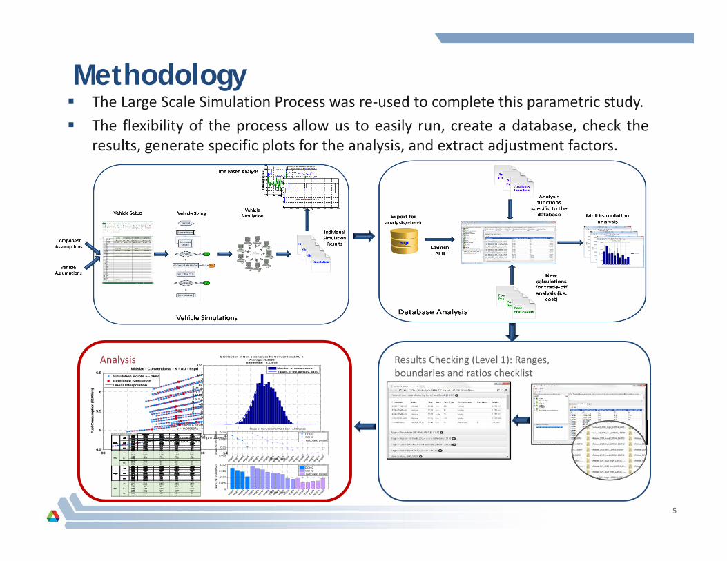
Methodology

5

The Large Scale Simulation Process was re‐used to complete this parametric study. The flexibility of the process allow us to easily run, create a database, check the

results, generate specific plots for the analysis, and extract adjustment factors.

Results Checking (Level 1): Ranges, boundaries and ratios checklist

Analysis

90 100 110 120 130 1404.5

5

5.5

6

6.5

M idsize/ Convent ional/y = 0:017313x + 4:037

Engine Power (kW)

Fuel

Con

sum

ptio

n (l/

100k

m) M idsize/ Convent ional / eng0

y = 0:01543x + 4:0914M idsize/ Convent ional/ ey = 0:014303x + 4:066

M idsize/ Convent ional/ ey = 0:010222x + 4:2919

M idsize/ Convent ional/y = 0:018696x + 4:0075M idsize/ Convent ional/y = 0:017214x + 4:0183

M idsize/ Convent iony = 0:016025x + 3:981

M idsize/ Convent ional/ eng6y = 0:014042x + 4:09M idsize/ Convent ional/ en

y = 0:013068x + 4:0478M idsize/ Convent ional / ey = 0:013025x + 4:0626M idsize/ Convent iona

y = 0:012108x + 4:0185M idsize/ Convent ional / ey = 0:0090205x + 4:2824M idsize/ Convent iona

y = 0:0082956x + 4:231

M idsize/ Convent ional/ ey = 0:0093124x + 4:1927M idsize/ Co

y = 0:0053066M idsize/ Coy = 0:005303M idsize/ Convent ional

y = 0:0065611x + 4:3528M idsize/ Convent ional/ eng16/ 109759/ Ay = 0:006687x + 4:2948

M idsize/ Convent ional/ eng17/ 103965/ A U / 6y = 0:0089611x + 3:7383

Midsize - Conventional - X - AU - 6spd

Simulation Points +/- 1kWReference SimulationLinear Interpolation

2.5 3 3.5 4 4.5 5 5.5 6 6.5 7 7.5-20

0

20

40

60

80

100

120

Fuel Consumption, l/100km

Num

ber o

f occ

uren

ces

Distribution of Non-zero values for Conventional-AU-6Average : 5.1699

Bandwidth : 0.13019

Number of occurencesValues of the density, x100

0.005

0.01

0.015

0.02

Engine Type

Slo

pe (

FC/

Eng

Pw

r)

eng0

1en

g02

eng0

3en

g04

eng5

aen

g5b

eng5

cen

g6a

eng6

ben

g7a

eng7

ben

g8a

eng8

ben

g12

eng1

3en

g14

eng1

5en

g16

eng1

7

Slope of Conventional AU 6 spd - All Engines

DOHCSOHCTurbo and Diesel

0

0.005

0.01

0.015

0.02

Engine Type

Slo

pe (

FC/

Eng

Pw

r)

eng0

1en

g02

eng0

3en

g04

eng5

aen

g5b

eng5

cen

g6a

eng6

ben

g7a

eng7

ben

g8a

eng8

ben

g12

eng1

3en

g14

eng1

5en

g16

eng1

7


Reminder: IAV Engine Technologies

6

Results

7

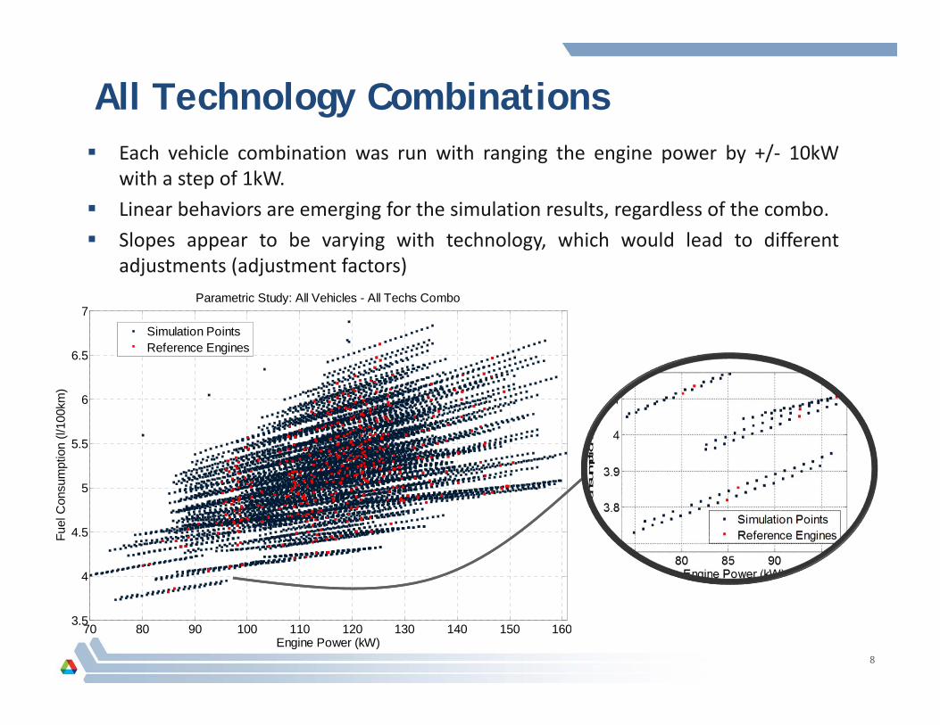
All Technology Combinations

8

Each vehicle combination was run with ranging the engine power by +/‐ 10kWwith a step of 1kW.

Linear behaviors are emerging for the simulation results, regardless of the combo. Slopes appear to be varying with technology, which would lead to different

adjustments (adjustment factors)

70 80 90 100 110 120 130 140 150 1603.5

4

4.5

5

5.5

6

6.5

7

Engine Power (kW)

Fuel

Con

sum

ptio

n (l/

100k

m)

Parametric Study: All Vehicles - All Techs Combo

Simulation PointsReference Engines

Evolution of Engine Technology - DOHC

9

Eng01 to Eng04: DOHC engines (refer to IAV engine report/description) One engine at a time / fixed engine – All Combos Improvement in engine technology appear to affect the parametric sensitivity as

the slope of the lines are reduced with lower highlighted regions.

80 100 120 140 1603.5

4

4.5

5

5.5

6

6.5

7

Fuel

Con

sum

ptio

n (l/

100k

m)

All Simulation PointsEng01

80 100 120 140 1603.5

4

4.5

5

5.5

6

6.5

7

Simulation PointsEng02

80 100 120 140 1603.5

4

4.5

5

5.5

6

6.5

7

Simulation Pointseng03

80 100 120 140 1603.5

4

4.5

5

5.5

6

6.5

7

Engine Power (kW)


Evolution of Engine Technology - SOHC

10

Eng5a to Eng8b: SOHC engines. Improved engines understandably provide lower fuel consumption results. The power span seems

to remain constant across engines, but rather fuel consumption is less sensitive to power change. Eng5a lines show an obvious bigger slope than Eng8b.

Constant

80 100 120 140 160

4

5

6

7

Fuel

Con

sum

ptio

n (l/

100k

m)

Simulation PointsEng5a

80 100 120 140 160

4

5

6

7

Engine Power (kW)

Simulation PointsEng5b

80 100 120 140 160

4

5

6

7

Simulation PointsEng5c

80 100 120 140 160

4

5

6

7


80 100 120 140 160

4

5

6

7

Engine Power (kW)


80 100 120 140 160

4

5

6

7


80 100 120 140 160

4

5

6

7


80 100 120 140 160

4

5

6

7


80 100 120 140 160

4

5

6

7


Evolution of Engine Technology – Turbo

11

Eng12 to Eng16: Turbo engines, Eng17: Diesel engine Turbo engines slopes lean towards flat behaviors. Diesel engine vehicles reveal the more fuel efficient and the least powerful vehicles, but

sensitivity seem to increase again as the slope gets steeper (Eng17)

80 100 120 140 160

4

5

6

7

Fuel

Con

sum

ptio

n (l/

100k

m)


80 100 120 140 160

4

5

6

7


80 100 120 140 160

4

5

6

7Engine Power (kW)


80 100 120 140 160

4

5

6

7

Engine Power (kW)


80 100 120 140 160

4

5

6

7


80 100 120 140 160

4

5

6

7


Evolution of Powertrain Technology

12

The breakdown per powertrain clearly shows the different operating powers as wellas the decrease in fuel consumption for progressive technologies (Conv. to CISG)

It has been established that the slope decreases moving downwards. Side note: It appears that similar fuel consumption results can be attained by using

different powertrain technologies along with the right tech. combo. for a given power.

70 80 90 100 110 120 130 140 150 1603.5

4

4.5

5

5.5

6

6.5

7

Engine Power (kW)

Fuel

Con

sum

ptio

n (l/

100k

m)

ConventionalMicroBISGCISG

Decreased Slope

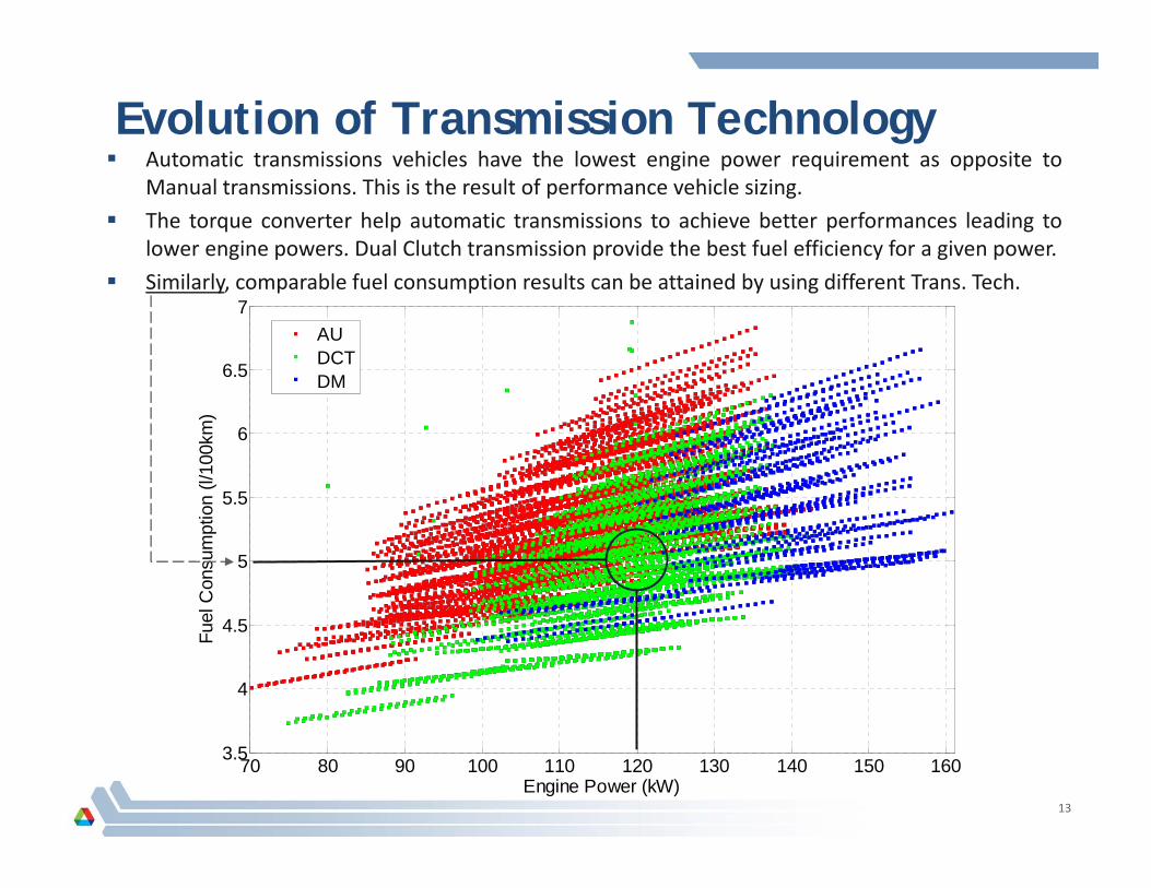
Evolution of Transmission Technology

13

Automatic transmissions vehicles have the lowest engine power requirement as opposite toManual transmissions. This is the result of performance vehicle sizing.

The torque converter help automatic transmissions to achieve better performances leading tolower engine powers. Dual Clutch transmission provide the best fuel efficiency for a given power.

Similarly, comparable fuel consumption results can be attained by using different Trans. Tech.

70 80 90 100 110 120 130 140 150 1603.5

4

4.5

5

5.5

6

6.5

7

Engine Power (kW)

Fuel

Con

sum

ptio

n (l/

100k

m)

AUDCTDM

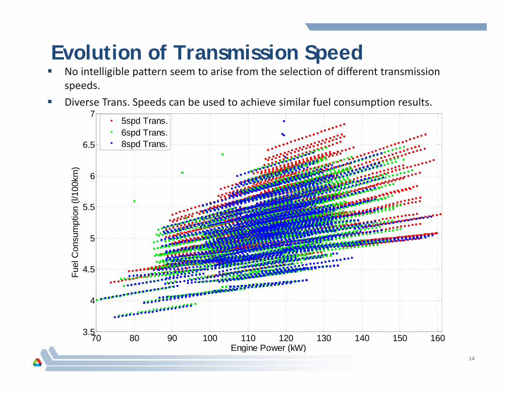
Evolution of Transmission Speed

14

No intelligible pattern seem to arise from the selection of different transmission speeds.

Diverse Trans. Speeds can be used to achieve similar fuel consumption results.

70 80 90 100 110 120 130 140 150 1603.5

4

4.5

5

5.5

6

6.5

7

Engine Power (kW)

Fuel

Con

sum

ptio

n (l/

100k

m)

5spd Trans.6spd Trans.8spd Trans.

Subset: Fixed Combo (All Pwt.)Eng01–AU–6 speed

15

Fuel consumption decreases with advanced powertrain Power Requirement decreases with advanced powertrain. The slope slightly decreases with advanced powertrain (very small impact)

85 90 95 100 105 110 115 120 125 130 1355

5.5

6

6.5


Engine Power (kW)

Fuel

Con

sum

ptio

n (l/

100k

m)

M idsize/ M icr o H ybr id/ eng01/ 118785/ A U / 6y = 0:016812x + 3:9131

M idsize/ M i ld H ybr id B I SG/ eng01/ 107877/ A U / 6y = 0:015763x + 3:8786

M idsize/ M i ld H ybr id CI SG/ eng01/ 95921/ A U / 6y = 0:015373x + 3:735

Midsize - X - Engine1 - AU - 6spd


Subset: Fixed Combo (All Pwt.)Eng01–AU–8 speed

16

Similar behavior (previous slide) is seen for different transmission speed selection.

85 90 95 100 105 110 115 120 125 1305

5.5

6

6.5


Engine Power (kW)

Fuel

Con

sum

ptio

n (l/

100k

m)

M idsize/ M icro H ybr id/ eng01/ 115309/ A U / 8y = 0:015377x + 4:0657

M idsize/ M ild H ybr id B I SG/ eng01/ 107877/ A U / 8y = 0:015351x + 3:9248

M idsize/ M ild H ybr id CISG/ eng01/ 97730/ A U / 8y = 0:015008x + 3:7765

Midsize - X - Engine1 - AU - 8spd


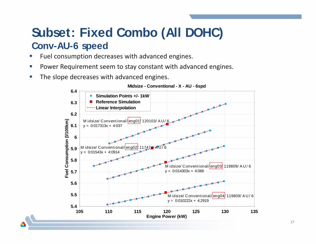
Subset: Fixed Combo (All DOHC)Conv-AU-6 speed

17

Fuel consumption decreases with advanced engines. Power Requirement seem to stay constant with advanced engines. The slope decreases with advanced engines.

105 110 115 120 125 130 1355.4

5.5

5.6

5.7

5.8

5.9

6

6.1

6.2

6.3

6.4


Engine Power (kW)

Fuel

Con

sum

ptio

n (l/

100k

m)






Subset: Fixed Combo (All SOHC)Conv-AU-6 speed

18

Similar trend (previous slide)

105 110 115 120 125 130 1355

5.5

6

6.5

M idsize/ Convent ional/ eng5a/ 120625/ A U / 6y = 0:018696x + 4:0075

Engine Power (kW)

Fuel

Con

sum

ptio

n (l/

100k

m)

M idsize/ Convent ional/ eng5b/ 120601/ A U / 6y = 0:017214x + 4:0183

M idsize/ Convent ional/ eng5c/ 122691/ A U / 6y = 0:016025x + 3:9814









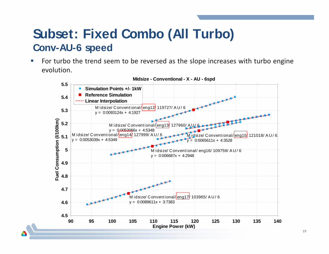
Subset: Fixed Combo (All Turbo)Conv-AU-6 speed

19

For turbo the trend seem to be reversed as the slope increases with turbo engineevolution.

90 95 100 105 110 115 120 125 130 135 1404.5

4.6

4.7

4.8

4.9

5

5.1

5.2

5.3

5.4

5.5


Engine Power (kW)

Fuel

Con

sum

ptio

n (l/

100k

m)








Slope Analysis – Fixed combo (All Engines)Conv-AU-6 speed

20

For DOHC and SOHC engines, advanced technologies are less sensitive to engine power variation. Sensitivitydecreases within each engine group as the slope is strictly decreasing (slope going down as the enginetechnology gets better).

Turbo engines slope values are overall lower than SOHC and DOHC engines. The engine is highly downsized andit is operating at high BMEP efficiency, hence a lower sensitivity level. However, the trend is not the same.

0.005

0.01

0.015

0.02

Engine Type

Slo

pe (

FC/

Eng

Pw

r)

eng0

1en

g02

eng0

3en

g04

eng5

aen

g5b

eng5

cen

g6a

eng6

ben

g7a

eng7

ben

g8a

eng8

ben

g12

eng1

3en

g14

eng1

5en

g16

eng1

7

Slope of Conventional AU 6 spd - All Engines


0

0.005

0.01

0.015

0.02

Slo

pe (

FC/

Eng

Pw

r)

eng0

1en

g02

eng0

3en

g04

eng5

aen

g5b

eng5

cen

g6a

eng6

ben

g7a

eng7

ben

g8a

eng8

ben

g12

eng1

3en

g14

eng1

5en

g16

eng1

7


Diesel Engine

Slope Analysis – Fixed combo (Turbo Engines)Conv-AU-6 speed

21

This area shows a normal trend from Eng12 toEng13 (decrease) and from Eng13 to Eng14

100 150 200 250 300 350 400 450 500 5500

50

100

150

200

Hot Efficiency Map (Torque) - Density energy

0.05 0.05 0.05 0.05 0.05 0.05 0.050.1 0.1 0.1 0.1 0.1 0.1 0.10.15 0.15 0.15 0.15 0.15 0.15 0.15

0.2

0.2

0.2 0.2 0.2 0.2 0.2 0.2 0.2

0.25

0.25

0.250.25 0.25 0.25 0.25 0.25 0.25

0.3

0.3

0.3

0.3

0.3

0.3 0.30.3 0.3

0.30.3

0.35

0.35

0.35 0.35 0.35

0.35

0.35

0.350.35

Engine Speed (RPM)

Torq

ue (N

.m)

energy density (%)EfficiencyTorque Max (N.m)Torque Min (N.m)Best Operating Line

% of total energy

0.5

1

1.5

2

2.5

3

3.5

4

5

6

7

8

9

10 x 10-3

Slo

pe (

FC/

Eng

Pw

r)

eng1

2

eng1

3

eng1

4

eng1

5

eng1

6

Slope of Conventional AU 6 spd - Turbo Engines

Turbo Engines

This area shows a suspicious trend from Eng14 toEng16 (increase in slope) due to data uncertainty.

Eng14 Eng15

It has been established that better efficiency engines lowers the slope.Eng14 shows a high efficiency region (data uncertainty/anomaly)compared to Eng15 leading to swap in the trend.

Note: Eng13 and Eng14 are equivalent, flat slopeis plausible (refer to IAV description)

1 2

Slope Analysis – All Pwt. (fixed combo)

22

The slope tend to slightly decrease with powertrain electrification, following the same logic: more efficient technologies, less fuel consumption sensitivity to power variation.

0

0.005

0.01

0.015

0.02

Engine Type

Slo

pe (

FC/

Eng

Pw

r)

Slope of All Powertrains - AU 6 spd - All Engines

eng0

1en

g02

eng0

3en

g04

eng5

aen

g5b

eng5

cen

g6a

eng6

ben

g7a

eng7

ben

g8a

eng8

ben

g12

eng1

3en

g14

eng1

5en

g16

eng1

7


0

0.005

0.01

0.015

0.02

Slo

pe (

FC/

Eng

Pw

r)

eng0

1en

g02

eng0

3en

g04

eng5

aen

g5b

eng5

cen

g6a

eng6

ben

g7a

eng7

ben

g8a

eng8

ben

g12

eng1

3en

g14

eng1

5en

g16

eng1

7


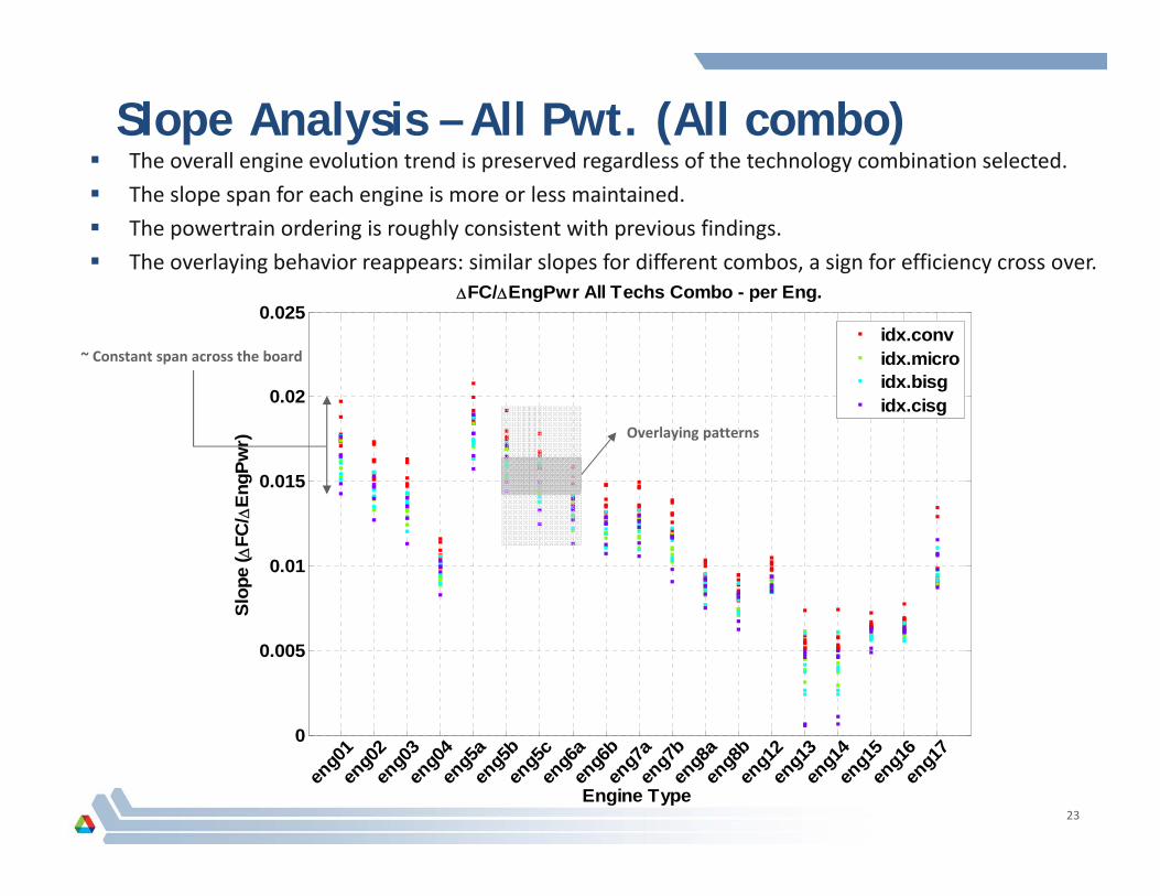
Slope Analysis – All Pwt. (All combo)

23

The overall engine evolution trend is preserved regardless of the technology combination selected. The slope span for each engine is more or less maintained. The powertrain ordering is roughly consistent with previous findings. The overlaying behavior reappears: similar slopes for different combos, a sign for efficiency cross over.

~ Constant span across the board

0

0.005

0.01

0.015

0.02

0.025

Engine Type

Slop

e (

FC/

EngP

wr)

eng0

1en

g02

eng0

3en

g04

eng5

aen

g5b

eng5

cen

g6a

eng6

ben

g7a

eng7

ben

g8a

eng8

ben

g12

eng1

3en

g14

eng1

5en

g16

eng1

7

FC/EngPwr All Techs Combo - per Eng.

idx.convidx.microidx.bisgidx.cisg

Overlaying patterns

Slope Analysis – All Pwt. (All combo)

24

Transmission technology change does not perturb the trending behavior, nor slope values (littleinfluence). The engine implication on the slope and therefore fuel efficiency is sustained.

The engine technology has a dominant effect on the results and the findings.

AUDCT

DM

0

0.005

0.01

0.015

0.02

0.025

eng03

eng5c

eng7b

eng13

eng17

eng02

eng5b

eng7a

eng12

eng16

eng01

eng5a

eng6b

eng8b

eng15

eng04

eng6a

eng8a

eng14

FC/EngPwr All Techs Combo - per Eng.

Slop

e (

FC/

EngP

wr)

Transmission Type

idx.convidx.microidx.bisgidx.cisg

Generation of Adjustment Factors are only relevant across powertrain and engine technology progress, especially engines.

Adjustment Factors – in %/10kW

25

Complete table: “ANL ‐ Eng. Param. Study ‐ Adjustment_Factors.xlsx” Subset: the table represents the percentage of fuel consumption adjustments needed for 10kW.

Units: %/10kW ‐‐‐‐‐‐ ∆Fuel. Cons. /∆ Eng. Pwr.Conventional Micro BISG CISG

Eng01

AU5 spd 3.33% 3.21% 3.34% 3.58%6 spd 3.14% 3.36% 3.16% 3.44%8 spd 3.19% 2.86% 3.14% 3.19%

DCT5 spd N/A. N/A. N/A. N/A.6 spd 3.29% 2.30% 3.31% 3.23%8 spd 3.31% 2.77% 3.28% 3.62%

DM5 spd 3.35% N/A. N/A. N/A.6 spd 3.28% N/A. N/A. N/A.8 spd 3.27% N/A. N/A. N/A.

Eng02

AU5 spd 3.07% 2.77% 3.05% 3.25%6 spd 2.84% 2.97% 2.92% 3.29%8 spd 2.89% 2.64% 2.90% 2.91%



Eng03

AU5 spd 2.92% 2.68% 2.90% 3.08%6 spd 2.72% 2.74% 2.78% 3.14%8 spd 2.77% 2.43% 2.69% 2.74%



Eng04

AU5 spd 2.17% 1.96% 2.20% 2.37%6 spd 2.01% 2.09% 2.13% 2.48%8 spd 2.07% 1.79% 2.07% 2.10%



Adjustment Factors – in l/100km/kW

26

Complete table: “ANL ‐ Eng. Param. Study ‐ Adjustment_Factors.xlsx” Subset: the table represents the amount of fuel consumption adjustments needed per unit of

power in kW. Units: l/100km/kW ‐‐‐‐‐‐ ∆Fuel. Cons. /∆ Eng. Pwr.Conventional Micro BISG CISG

Eng01

AU5 spd 0.0196 0.0178 0.0175 0.01756 spd 0.0172 0.0170 0.0158 0.01568 spd 0.0171 0.0155 0.0153 0.0147

DCT5 spd N/A. N/A. N/A. N/A.6 spd 0.0177 0.0191 0.0162 0.01748 spd 0.0172 0.0156 0.0167 0.0164

DM5 spd 0.0191 N/A. N/A. N/A.6 spd 0.0178 N/A. N/A. N/A.8 spd 0.0180 N/A. N/A. N/A.

Eng02

AU5 spd 0.0172 0.0152 0.0155 0.01546 spd 0.0153 0.0147 0.0141 0.01398 spd 0.0151 0.0137 0.0138 0.0131



Eng03

AU5 spd 0.0161 0.0141 0.0146 0.01436 spd 0.0142 0.0134 0.0130 0.01288 spd 0.0141 0.0125 0.0126 0.0117



Eng04

AU5 spd 0.0116 0.0100 0.0108 0.01066 spd 0.0102 0.0099 0.0096 0.00978 spd 0.0101 0.0091 0.0094 0.0087



Distribution of Adjustment Factors

27

Most of the percentage values stand around 3%, still a reasonable number of vehicles show percentage at around 2% and 1.5%.

Those 3 groups of percentages mimic the 3 engine categories (DOHC, SOHC and Turbo) we demonstrated in the previous slides.

-1% 0% 1% 2% 3% 4% 5%0

5

10

15

20

25

30

35

Percentage Adjustement per 10kW (%/10kW)

Num

ber o

f Occ

uren

ces

Distribution of Correction Factors in % for every 10KW of Engine Power VariationAverage : 2.3235

Bandwidth : 0.17602

Nb of Occurences - All Tech. Combos.Density

Conclusion

28

A parametric study was done on multiple vehicle tech. combinations by varying areference engine power over a range of +/‐ 10kW with a step of 1kW.

The impact of engine power on fuel consumption results was assessed to mimicengine inheritance effects.

Each vehicle combination selected required extra 20 simulation, resulting to atotal of 14,000 points.

Change in engine power leads to linear impact on fuel consumption with relationdepending on engine technology and powertrain configurations (minimal).

It has been demonstrated that vehicle fuel consumption sensitivity to powerchange is mainly influenced by the powertrain and the engine technology.Transmission technology and speed selection have little to no impact.

It has been proven that the ∆Fuel Consumption/∆Engine Power (the slope of theparametric study points) minimally decreases with advances in powertrain orengine technology (better efficiency levels). The slope is the sensitivity levelrepresenting how much engine power variations affect fuel consumption results.

Adjustment factors have been generated to allow vehicle fuel consumptionadjustments with possible future change in engine powerrequirement/performance requirement.

For DOT/VOLPE nd - National Highway Traffic Safety ... linear proprieties such as Mass, Aerodynamic...

Documents

Transcript of For DOT/VOLPE nd - National Highway Traffic Safety ... linear proprieties such as Mass, Aerodynamic...