Teachers Mannual

WATER RESOURCES DEVELOPMENT (HYDROPOWER DEVELOPMENT)

for

Engineering Degree Programme Elective Course (for Branches in Electrical/ Mechanical / Instrumentation/ Electronic Engineering)

For Department of Technical Education Govt. of Uttarakhand

ALTERNATE HYDRO ENERGY CENTRE INDIAN INSTITUTE OF TECHNOLOGY, ROORKEE

July 2007

PREFACE

Lecture notes for the proposed Engineering Degree Level Course entitled ‘Hydro

Development’ for branches in Electrical, Mechanical, Instrumentation and Electronic

Engineering is in accordance with the approved syllabus. The notes are based on actual

design of large and small hydropower station by Prof. O. D. Thapar who designed hydro

stations from micro hydel to the largest in India for over 50 years (1956 – to date).

Citation by Institution of Engineers (India). Roorkee Local Centre to Prof. O. D. Thapar

is at the end of these notes. Modern trends in design are brought out. Copies of some

relevant published/unpublished papers on various aspects of design are included. It may

be noted that published design papers are relevant to the design practice at the time of

publication/design and must be used/modified with relevant to current practice as per

references given in the text. The material in these notes is also part of a book entitled

‘Hydro-electric Engineering Practice in India’ being complied by author.

(ARUN KUMAR) HEAD, AHEC, IIT, ROORKEE

AHEC-IITR/Ua. Govt./syllabus/WR-HPD/May 2006

FOR ENGINEERING DEGREE LEVEL ELECTIVE COURSE For Branches in Electrical, Mechanical, Instrumentation, Electronics Engineering 1. Subject Code: Course Title: Hydropower Development 2. Contact Hours: L: 48 T: 0 P:0 3. Examination Duration (Hrs.): Theory: Practical: 4. Relative Weightage: CWS PRS MTE ETE PRE 5. Credit: 6. Semester: Autumn Spring Both 7. Pre-requisite: NIL 8. Subject Area: 9. Details of Course: Sl. No. Particulars Contact

Hours 1. INTRODUCTION: Type of Hydroelectric development, classification,

Techno Economic studies for capacity size & type. 7

2. Hydraulic Turbines and Governor: Types; selection criteria, Model testing, specifications. Speed rise and Pressure Rise, studies for performance requirements.

9

3. Hydro Generator and Excitation System: Types; selection; Characteristics; Specification; Testing

4

4. Power Transformer: Types; Characteristics; Specification and Testing 2 5. HV Circuit Breaker: Types; Characteristics; Specification and Testing 3 6. Power evacuation arrangements; main single line diagram; interconnected

with grid 3

7. Control & Protection: Protective Relaying and Metering of Hydro Generators; Turbines, Transformers, Bus Bars and Outgoing Feeders, control and Monitoring System for Turbines, Generators, Exciters; transformers; Breakers, Power Plant Start/Stop, running control and Annunciation

12

8. Electrical Auxiliaries: Auxiliaries Power; DC System; Power & Control Cables and Cabling; Lighting System; Grounding System

6

9. Mechanical Auxiliaries: EOT Crane; Cooling Water System; Dewatering and Drainage System; HP & LP compressed Air System; Fire Protection; Ventilation and Air conditioning

6

10. Switchyard Equipment: Isolators, Potential Transformers, Current Transformer; Lighting Arrestors; Switchyard and Structures

3

11. Erection, Commissioning and Field Testing Renovation and modernization 2 Suggested Readings:

1. Hydro Plant Electrical System – by David M. Demon 2. Mechanical Design of Hydro Plants – American Society of Mechanical Engineers 3. Water Power Development – by Masony 4. Hydro-Electric Engineering PRACTICE – by J. Gutterie Brown – Vol. II E & M 5. USBR Design Memorandum and Standards 6. Army Corps of Engineer Design Standard 7. IEEE & IEC standards (Relevant) 8. BIS Standards (Relevant)

1-1

Chapter-1

Techno Economic Considerations – Type, Capacity and Unit Size

1.1 General The major electro-mechanical components of power plant are the inlet valve/gate, turbine, draft tube, generator, control and protection equipment and substation for transformation of power to the transmission line voltage. In terms of space requirement and cost the major items are the turbine and generator. Mechanical auxiliary system include EOT crane, drainage and dewatering systems, cooling water system, high pressure, low pressure compressed air system, water level measuring and transmitting device, oil filtration, fire protection system and ventilation and air conditioning system. Electrical auxiliary systems include auxiliary power system including station transformers. DC system including station batteries, battery chargers and DC distribution system, lighting system, power and control cables, cabling including cable racks, grounding mat and grounding system, internal communication system. Selection of Equipment, their Characteristics and Specifications for design of hydro power station depends upon type of hydro electric development and classification with respect to head and size. 1.2 Types of Projects Capacity and unit size depends upon the type of project. There are two main types of hydropower schemes that can be cateigorized in terms of how the flow at a given site is controlled or modified. These are: 1. Run-of-river plants (no active storage); and 2. Plants with significant storage In a run-of-river project, the natural flow of the river is relatively uncontrolled. In a storage project, the filling and emptying of the impounded storage along with the pattern of the natural stream flow controls the flow in the river downstream from the storage impoundment. Run-of-river plants can be located at the downstream end of a canal fall, open flume, or pipeline diverting the stream’s flow around a water supply dam or falls. The available flow governs the capacity of the plant. The plant has little or no ability to operate at flow rates higher than that available at the moment. In a conventional plant, a dam, which stores water in a reservoir or lake impoundment, controls the river flows. Water is released according to electric, irrigation, water supply, or flood control needs. Constructing a dam and storage reservoir can increase the

1-2

percentage of time that a project can produce a given level of power. Base load plants-those operated at relatively constant output-may have either a small capacity relative to the river flow or may have a significant storage reservoir. Storage reservoirs can be sized for storing water during wet years or wet seasons. Alternatively, they can be sized to provide water for weekly or daily peak generation. A storage reservoir allows using available energy that might otherwise be wasted as spill. Plants with storage at both head and tailrace are pumped storage project and are not discussed in these notes. 1.2.1 Run of the River Schemes or Diversion Schemes This type of development aims at utilizing the instantaneous discharge of the stream. So the discharge remain restricted to day to day natural yield from the catchments; characteristics of which will depend on the hydrological features. Diurnal storage is sometime provided for optimum benefits. Development of a river in several steps where tail race discharges from head race inflows for downstream power plants forms an interesting variation of this case and may require sometimes special control measures. Small scale power generation also generally fall in the category and may have special control requirement especially if the power is fed into a large grid. 1.2.2 Storage Schemes In such schemes annual yield from the catchment is stored in full or partially and then released according to some plan for utilization of storage. Storage may be for single purpose such as power development or may be for multi purpose use which may include irrigation, flood control, etc. therefore, design of storage works and releases from the reservoir will be governed by the intended uses of the stored water. If the scheme is only for power development, then the best use of the water will be by releasing according to the power demand. Schemes with limited storage may be designed as peaking units. If the water project forms a part of the large grid, then the storage is utilized for meeting the peak demands. Such stations could be usefully assigned with the duty of frequency regulation of the system. 1.2.3 Synchronous Condenser operation Motoring of a conventional hydro-electric units is desired so that unit can be utilized as a synchronous condenser for electric system enhancement by supplying or absorbing reactive power or for the unit to be in spinning reserve for rapid response to system needs. For this purpose, the generating unit is started in the normal way upto speed no load position, synchronosed with the grid and turbine wicket gates are then closed. Draft tube water depression system is utilized in these hydro -electric unit to depress the water below the runner of the turbine. By depressing the water below the runner, it allows the unit to be motored with minimum power consumed from the system since it is spinning in air as opposed to water.

1-3

1.2.4 Pump Storage Scheme Principle The basic principle of pumped storage is to convert the surplus electrical energy available in a system in off-peak periods, to hydraulic potential energy, in order to generate power in periods when the peak demand on the system exceeds the total available capacity of the generating stations. By using the surplus scheme electrical energy available in the network during low-demand periods, water is pumped from a lower pond to an upper pond. In periods of peak demand, the power station is operated in the generating mode i.e. water from the upper pond is drawn through the same water conduit system to the turbine for generating power. There are two main types of pumped storage plants:

i) Pumped-storage plants and ii) Mixed pumped-storage plants.

Pump-storage plants In this type only pumped storage operation is envisaged without any scope for conventional generation of power. These are provided in places where the run-off is poor. Further, they are designed only for operation on a day-to-day basis without room for flexibility in operation. Mixed pumped-storage plants In this type, in addition to the pumped storage operation, some amount of extra energy can be generated by utilizing the additional natural run-off during a year. These can be designed for operation on a weekly cycle or other form of a longer period by providing for additional storage and afford some amount of flexibility in operation. 1.2.5 Components The main components of hydro-electric unit including pumped-storage plants with reversible generator/motor units are, as follows an show in fig. Fig. 1.2.5.1.

i) the upper reservoir ii) intake iii) Pressure water System including penstocks, surge tanks etc. iv) pump/turbine with governor v) draft tube gate vi) the tail race the lower reservoir level monitoring vii) generator/motor with exciter and cooling

1-4

viii) generator/motor terminal equipment ix) pump starting equipment phase reversal x) Circuit breaker xi) Step up unit transformer xii) Station service transformer

1.3 Unit Size Classification Design of hydro power plants and selection of equipment is impacted by the size of the power plant. For this purpose hydropower plants are classified as medium and large or small Hydel power plants. Defined unit size and installed capacity varies in different countries. For the purpose of equipment selection and design the following classifications are considered in these notes. a) Medium and Large hydros

i) Medium Hydros – 5000 kW to 25000 kW unit size ii) Large Hydros – above 25000 kW unit size

b) Small Mini & Micro Hydel Plants are classified as follows:

i) Micro Hydro up to 100 kW unit size ii) Mini Hydros – 100 kW to 1000 kW unit size iii) Small Hydros - 1000 kW to 5000 kW unit size. International Electro

Technical Commission (IEC) - Small hydro equipment guide (IEC-1116) is for unit size upto 3000 kW.

In India 25,000 kW is classified small Hydro. 1.4 Techno-Economic Studies Techno-economic studies are required to be carried out to determine power plant capacity and unit size. Type of power plant and its interconnection with the grid affects characteristics and equipment selection. Plant capacity is dependant upon site data as regard effective head and flow. Interconnecting grid characteristics and operation of the plant impact size, capacity and characteristics of equipment. Preliminary pre-investment economic studies are carried out to determine whether detailed feasibility studies are required.

1-5

Note –1 For reversible (pump storage) Units Only Note –2 For Synchronous condenser operated unit

Fig. 1.2.5.1 Major Components of a Hydroelectric Unit

1-6

1.4.1 Site Data

The basic data for selection of hydraulic turbine are the design flow of water and the net head on turbine. For interconnection with the grid data regarding size of grid and nearest location of grid substation and its voltage is required.

The initial input for the process is determining: (a) The hydraulic resource or river/canal/stream flow, and (b) The economic criteria to evaluate the project economic feasibility, including the value of energy, value of capacity, escalation rates, discount rate, etc. The project hydraulic data (water availability versus time) is obtained by reviewing historical records or estimated by other techniques. As a result of this analysis, an initial plant capacity is assumed. A trial number of turbines-generator units is also assumed at this stage. The next step is to determine, performance characteristics of the selected turbines and generators. Such characteristics are used in calculating the annual energy from the plant and its capacity. Outline dimensions of the turbines, generators and other major equipment are used to estimate the powerhouse dimensions and costs. Economic analysis for a range of possible alternatives typically are conducted for the various capacities, annual generation, capital costs and economic criteria. If the project appears feasible, other plant capacities and alternative machinery solutions would be evaluated in the same manner until the optimal plant capacity is determined. If the initial plant capacity is not feasible, smaller capacities would be evaluated in a similar manner. After evaluating several alternatives, a range of solutions available for consideration can provide the potential developer with a basis for selection. Maximum utilization of available potential energy from the energy resource is required depending upon present economic viability. Accordingly energy remaining unutilized and efficiency of operating equipment is an important consideration in deciding the number and size of generating units. Further rising cost of energy demands provision to be made for further capacity addition to utilize this unutilized energy during seasonal excess water periods. In case of unit size above 5 MW, plant capacity, unit size may also be determined on the basis of capacity in peaking station. Following site conditions may affect the design of the powerhouse and the equipment. (a) Quality of water e.g. amount and size of sediments carried by the water in

the area around the water intake or downstream of the desilting works; the presence of any living organism and any dissolved chemicals.

(b) Local conditions; extremes of air temperature, humidity etc. (c) Transport or access limitations.

1-7

1.4.2 POWER EQUATION

Power can be developed from water whenever there is available flow, which may be utilized through a fall in water level. The potential power of the water in terms of flow and head can be calculated with the following equation.

kW = 9.804 x Q x H x E

Where :

Q is quantity of water flowing through the hydraulic turbine in cubic meters per second.

H is available head in meters E is the overall efficiency an overall turbine, generator, station use and deterioration, and transformer efficiency of 85% can be used for estimating the energy from a flow duration curve. Whenever the flow rate and/or the head vary, a more precise analysis of the efficiency of the hydraulic turbine is required. A value of 95% may be used for all other losses including generator, station use and deterioration, and transformer. Therefore, the total efficiency to be used in the power operation studies is the product of the turbine efficiency and all other losses (0.95). If the turbine and generator are coupled together with a speed increaser, the losses, other the turbine, may be estimated as 93%. 1.4.3 CAPACITY AND UNIT SIZE Plant Rating -Water power studies determine the ultimate plant capacity and indicate the head at which that capacity should be developed. Techno-economic (optimization) studies are required to be carried out to determine optimum size and number of units to be installed. Considerations involved in determining generating capacity to be installed and optimum number and size of units to be selected at the site are as follows:

(a) Maximum utilization of energy resource. (b) Maximum size of units for the net head available. (c) Operating criteria. (d) Spare capacity (e) Optimum energy generation and cost of generation per unit. (f) Part load operation (g) World wide and local experience. (h) Future provision

The generating capacity of a hydro power plant is usually expressed in kiloWatt (kW) or megawatts (MW) and is selected based on a careful evaluation of several important parameters i.e. head, discharge and head flow combination.

1-8

1.4.4 INTERCONNECTION WITH GRID Installed capacity, unit size, characteristics and design of the hydro plant are impacted by interconnected with grid. Installed capacity depends upon feasible peaking capacity requirement, spare capacity to be provided in the proposed power house for maintenance, spinning reserve and forced outages. 1.4.5 OPERATING CRITERIA

Operating conditions and constraints affect the Electro-mechanical equipment and power station design.

(a) Following hydraulic conditions affect the design of the unit and the plant:

i) Maximum allowable up and down surges in the channel. ii) Head Variation in the Headrace and Tailrace.

(b) Operational constraints e.g. multipurpose scheme, environmental, fisheries etc. (c) Attended or unattended operation and type of manpower available for O & M. (d) Electrical conditions for plant operation e.g. isolated operation, parallel operation,

grid connected (type of grid weak or strong). (e) Whether peaking operation required. 1.5 Pre-Investment Economic Studies 1.5.1 Methodology

The methodology for the pre-investment described with special reference to small hydros upto 10 MW because these hydros are not multi purpose. For large multi purpose hydro schemes suitable variations can be made.

1.5.2 Pre-Investment Study: Tasks

The components identified as important in pre-investment studies are shown in figure-1.5.2. The tasks include those required to establish the economic feasibility (power potential, value, cost, and site capabilities) and those that should aid in defining and assessing critical issues quantitatively.

1.5.3 PLAN RECONNAISSANCE STUDY

The specific scope and purpose of the study should be defined and needed output products identified. The scope and purpose of this report is identified as pre-investment feasibility.

1-9

1.5.4 CONTACT PRINCIPAL AGENCIES Ministry of Energy (CEA) is responsible for large hydros. The ministry of non-conventional energy sources (MNES) is responsible for small hydros upto 25 MW. Specific programmes designed to encourage the development of hydroelectric are available. Each state has also issued guidelines for encouraging participation of private sector in this development. The terms and conditions for implementing small hydropower in private sector including arrangements for purchase of power, banking etc. have also been notified by most states. 1.5.5 SCOPE OF ECONOMIC EVALUATION Unless developed in clusters, small hydro projects are generally single purpose power projects. As such, the economic justification is based on the value of power that can be generated. If other project features are to be considered in the economic evaluation such as tourism, recreation, fish etc., they should be defined at this point and tasks related to their quantification formulated. 1.5.6 DEFINE POWER POTENTIAL The value of power output from a proposed project, and the appropriate physical facilities are sensitive to the nature of the power potential. Is the plant likely to produce only energy or does it have potential for dependable capacity value as well ? About how much output is likely and what is its variability. These are information items that are needed to assess market potential and provide formulation data. 1.5.7 ASSESS MARKET POTENTIAL Potential buyers of power output should be identified so that value of power may be determined. Information important to determine the value of power includes: who is presently generating and selling power in the area, what types of generating equipment are in operation, and who are the major customers. Purchasers could include utilities, cooperatives, private industry and other institutions. 1.5.8 ESTIMATE POWER OUTPUT The value of power output and the cost of works to produce the power are functions of the magnitude and character of output. Several project installed capacities should be investigated to estimate power potential, covering a range of likely installed capacities. Three potential sizes would seem appropriate. A mid value of installed capacity chosen to correspond to the 25% flow-exeedence value is a reasonable starting point with the other two selected at say 15% and 35% exceedance values.

1-10

Figure 1.5.2- Important Components of study

1-11

The desired product of this task is an array of installed capacities and corresponding annual energy output,indicators of the range of likely output by seasons and years (high and low flow periods), and an assessment as to the amount of capacity (if any) that might be credited as dependable. The head and flow ranges of the array are likewise needed to cost the power features. 1.5.9 DEVELOP SPILLWAY HYDROLOGY The flood flows that must be passed, and the spillway capability to pass the flood events of rare occurrences are important for the design of the spillway. 1.5.10 IDENTIFY PHYSICAL WORKS The power Generation and appurtenant works must be suitable to the intended installation and site. A specific preliminary design is not required but sufficient formulation to define likely machine type and possible configurations are needed to assess site issues, and to provide a basis for cost estimates. 1.5.11 FORMULATE AND COST PROJECT Cost estimate for construction, site acquisition, operation and maintenance, and engineering and administration are needed to assess economic feasibility. To facilitate pre-feasibility estimates, available data on actual costs of projects recently constructed and data contained in Guide Manual entitled "FEASIBILITY STUDIES FOR SMALL SCALE HYDRO POWER ADDITIONS" issued by the INSTITUTE FOR WATER RESOURCES; USA and IEC 1116 "INTERNATIONAL STANDARD" electromechanical equipment guide for small hydroelectric installations have been analyzed to develop, charts and tables contained in this report. Figure-1.5.11 provides a basis for estimating the major share of construction costs in SHP for items that are governed by capacity and head, e.g., turbine, generator, and supporting electrical/mechanical equipment. The chart was developed by studying the generator and powerhouse costs for a variety of turbine types for a complete set of head/capacity values. The chart is, therefore, the locus of least cost points for head/capacity values shown. The reader is cautioned that this chart is based on the figures contained in other reports and least construction cost criteria governed for a site, site issues of space and configuration, and generation issues of performance ranges were not used. The chart should be adequate, however, for pre-feasibility estimates. Installation of multiple units can be considered using these charts although the reinforcement of analysis might be questionable at this level of study. The multiple units may be critical to small hydro feasibility because of the goal of generating as much energy as possible from the available flow regime. Projects approaching the upper limits of small hydro capacity (5 MW) probably warrant using more detailed pre-feasibility level of study. The remaining components needed for preparing construction cost estimates are included in table - 2.1(A, B & C). Other cost items that may have surfaced during study of the critical issues (access etc.) should be estimated at this stage as well. In the absence of specific estimates for these additional items, uniform expenses allowance of up to 20% would be appropriate. The

1-12

products of this task should be an array of costs for the range of installed capacities for which power estimates are prepared.

Figure 1.5.11 Cost Estimate based on Capacity and Head NOTES: 1 Estimated costs are based upon a typical or standardized turbine coupled to a

generator either directly or through a speed increaser, depending on the type of turbine speed.

2 Costs include Turbine/generator and appurtant equipment, station electric equipment

miscellaneous power plant equipment, powerhouse civil works including, excavation, tailrace, switchyard civil works, upstream slide gate, and construction and installation.

3 Costs not included are transmission line, penstock, construction and switchyard

equipment. 4 Cost base April 1997. 5 The transition zone occurs as unit type changes due to increased head.

1-13

6 For a multiple unit power house additional station equipment cost are 14 lacs + 4 0

lacs (n-1) where n is the total number of unit.

For micro hydropower Projects (upto 100 kW unit size), cost estimates may be based on Table- 1.1

Table - 1.1 Project Cost Estimates (Micro Hydel Projects) Micro Hydel Upto 100 kW Cost including turbine, generator, electronic load controller with hot water system or ballast load; Power and control equipment, Power house and tail race structure, etc.

Rs. 40,000 per kW

These units are proposed to be equipped with Non Flow Control turbines designed for runaway conditions and controlled by Shunt Load Governor (Electronic Load Controllers). The penstocks are designed for no water hammer conditions. The figure provides cost estimates for generating unit, power house diversion etc. Other components need to be added. Construction cost estimates for micro hydel projects are indicated in table -1.2. TABLE - 1.2 MISCELLANEOUS PRE-FEASIBILITY ESTIMATE COSTS (Cost base April 2000) (A) PENSTOCK COST Effective head (Meter) 3 6 16 30 60 100 200

Cost Index (CI) 7.7 3.80 1.6 0.9 0.44 0.28 0.18

Installed cost (Rs in lacs) = CI x Penstock length (m) x Installed capacity (MW) N.B.: For Micro hydel (upto 100 kW) with Shunt Load (Electronic Load) Governor the Installed cost will be 50% less

(B) SWITCHYARD EQUIPMENT COST (Rs. in lacs) Plant Capacity (MW)

Transmission Voltage (in KV)

11 KV

33 KV

66 KV

132 KV

1-14

1 25 30 55 80 3

45

50

60

90

5

55

65

75

105

10

75

85

105

140

(C) TRANSMISSION LINE COST (Rs. in lacs) Plant Capacity (MW)

length of transmission line (in Km)

1.5 Km

3 Km

10 Km

16 Km

24 Km

0.5

10

20

60

--

--

5.0

16

28

64

130

180

10

20

36

72

140

220

1.5.12 COST STREAMS The construction cost values developed in the previous paragraph need to be gathered, organized and analysed to permit expeditious performance of the economic feasibility calculations. The construction costs should be escalated to the study date. It is recommended that the national capital cost index be used for uprating as a composite value for all items for the pre-investment cost estimates. Cost estimates are also needed for the non-physical works cost items. An allowance for unforeseen contingencies ranging from 10% to 15% should be added to the sum of the construction costs, the value depending upon a judgment as to the uncertainties. A mid value of 15% for contingencies is appropriate in the absence of more detailed analysis. All investigation, management, engineering and administration costs that are needed to implement the project and continuation of its services are appropriately included in the pre-investment determination, engineering, interest during construction, etc., of 15-20% be added. Total indirect costs to be added will therefore vary between 25% and 30%. Notes 1. Estimated costs are based upon a typical or standardised turbine (non flow control)

coupled to generator either directly or through belt drive. 2. Costs include turbine/generator ; Shunt load governor (Electronic load controller);

Power house ; Inlet wheel valve, Water ballast load; Construction and installation. 3. Penstocks/Channel; distribution lines costs etc are not included. Refer Table 1 for

these costs. 4. Cost base date: April 2000.

1-15

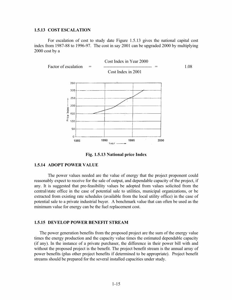
1.5.13 COST ESCALATION For escalation of cost to study date Figure 1.5.13 gives the national capital cost index from 1987-88 to 1996-97. The cost in say 2001 can be upgraded 2000 by multiplying 2000 cost by a Cost Index in Year 2000 Factor of escalation = --------------------------------- = 1.08 Cost Index in 2001

Fig. 1.5.13 National price Index 1.5.14 ADOPT POWER VALUE The power values needed are the value of energy that the project proponent could reasonably expect to receive for the sale of output, and dependable capacity of the project, if any. It is suggested that pre-feasibility values be adopted from values solicited from the central/state office in the case of potential sale to utilities, municipal organizations, or be extracted from existing rate schedules (available from the local utility office) in the case of potential sale to a private industrial buyer. A benchmark value that can often be used as the minimum value for energy can be the fuel replacement cost. 1.5.15 DEVELOP POWER BENEFIT STREAM The power generation benefits from the proposed project are the sum of the energy value times the energy production and the capacity value times the estimated dependable capacity (if any). In the instance of a private purchaser, the difference in their power bill with and without the proposed project is the benefit. The project benefit stream is the annual array of power benefits (plus other project benefits if determined to be appropriate). Project benefit streams should be prepared for the several installed capacities under study.

1-16

1.5.16 DETERMINE ECONOMIC FEASIBILITY Economic feasibility is positive when the stream of benefits exceeds the stream of costs. It is suggested that the Internal Rate of Return method of characterizing project feasibility is employed. The Internal Rate of Return is the discount rate at which the benefits and costs are equal, e.g., the discount rate at which the benefit to cost ratio is unity. This avoids the need at the pre-investment stage to adopt a discount rate and thus provides an array of economic feasibility results. The analysis should be performed for each of the installed capacities under study. The alternative is to compute a benefit cost ratio using the discount rate that represents the minimum attractive rate of return for the project proponent. An example computation and display is elaborated in the end of this chapter. Should the outcome of the economic feasibility test appear uncertain, simple sensitivity analysis based on the important variables (power values/fuel costs, amount of energy/capacity, etc.) could significantly contribute to narrowing the band of uncertainty. 1.5.17 IDENTIFY CRITICAL ISSUES The potentially critical issues should be identified and action required to clarify their importance defined. The issues have been generally identified in this section but important variations may exist depending on project proponent, prior studies, location, etc. The issues that are likely to emerge are primarily related to legal and institutional factors and physical factors focused on the site. 1.5.18 ASSESS LEGAL/INSTITUTIONAL ISSUES An assessment is needed at the pre-feasibility stage to define the mechanisms that are likely to be needed to implement a project (e.g. site ownership, legal authority to develop/sell power, access to power grids) and to appraise the action needed to overcome obstacles, should they exist. 1.5.19 ASSESS SITE ISSUES A site visit should be considered essential at this stage for (rare exceptions excluded) all pre-feasibility investigations of projects. Sketches and drawings may be made and/or existing ones verified defining space for plant siting, terrain and construction features, operational status of facilities, and other items pertinent to the physical arrangement of the site, construction of the needed works, and transmission of the power to distribution facilities. The site visit by responsible professionals should be coordinated to provide for a reconnaissance stage integrity assessment as well. 1.5.20 ASSESS FINANCIAL ISSUES Sufficient funds must be raised to construct the plant and adequate flow of revenues generated to provide for maintaining the plant in service, retiring loans, and producing a profit to the developer. The nature of likely financing needs to be defined, potential

1-17

marketing and revenue arrangements described, and perhaps most important at this pre-investment stage, the probable cost of capital (interest rate of financing) determined. 1.5.21 DOCUMENT PRE-INVESTMENT FINDINGS The findings of the pre-investment investigation should be documented for study by responsible authorities (public officials, boards of directors, private investors etc.); supporting studies, facts, and references described and codified to expedite performance of further studies; and should the finding be positive, a plan of action for the next steps outlined for execution by the project proponent. 1.5.22 TIME, COST AND RESOURCES FOR RECONNAISSANCE STUDIES The time, cost, and manpower resources required to perform pre-investment studies for small hydroelectric power plants will vary depending on expected plant size, site conditions, specific scope and depth of study, and availability of information (prior resource assessments and screening studies). 1.5.23 EXAMPLE PRE-FEASIBILITY ECONOMIC ANALYSIS PLANT

CHARACTERISTICS: Run of River Scheme Head = 40 meter Penstock = 100 m Capacity = 4 MW Transmission = 5 lacs Efficiency = 80% Economic life = 25 Years Evaluation Date = 1997 Average Yearly- Energy Generated = 12.6144 MU Selling Price = Rs. 2.25/unit Investment Cost Rs. in lacs Turbine, Generator and Civil (Figure – 1.9.11) 900 Additional Station, Equipment (Multi-unit) Penstock (Table-1.2 (A) 288 Switchyard Equipment (Table-1.2 (B) 58 Transmission Line (Table-1.2 (C) 65 Others (access, miscellaneous site construction) --

1-18

Subtotal 1311 Escalation (April, 96 to April, 97 - figure – 1.9.13) --- Contingencies at 10% - 20% 131.1 Subtotal 1442.10 Indirect @ 20% 262.2 Total Investment Cost (IC) 1704.3 CAPITAL RECOVERY FACTOR : The factor used to calculate the annual amount to be charged to project to recover capital investment. r(1+r)n Capital Recover Factor = ---------------- (1+r)n - 1 r - interest rate n - life of project ANNUAL COST : Annualized Investment Cost is a function of discount rate and economic life of a project and is computed by multiplying the Total Investment Cost by the Capital Recovery Factor for the discount rate and economic life selected (See Table below 1.3). The reconnaissance economic feasibility for the example is shown graphically in Fig. 1.5.23 (a) and Fig. (b). OPERATION AND MAINTENANCE (O&M) COST @ 2% = 34.08 Total Annual Cost (sum of Annualized Investment Cost and O & M cost) and Total annual benefits have been calculated in the following Table 1.3.

1.6 Economics

Cost of Generation Since pumped storage plants are generally negative energy projects, the method of working out the cost of generation for the conventional hydro scheme cannot be adopted for the pumped storage projects.

1-19

Table 1.3 : COST AND BENEFIT COMPUTATION TABLE

Discount Interest Rate (%)

Capital Recovery Factor

Annualized Investment Cost in Lacs (Col 2 x IC)

Total Annual Cost in Lacs (Col 3 + O&M Cost)

Break Even Energy Value Rs./kWH (Col 4/ Energy Generation)

Total Annual Benefit in Lacs (Energy Generation x Selling rate)

Net Benefit in Lacs (Col 6 - Col 4)

B/C Ratio (Col 6 / Col 4)

1 2 3 4 5 6 7 8 12% 0.1138 193.98 228.06 1.81 283.824 55.76 1.24 14% 0.1276 217.48 251.56 1.99 283.824 32.26 1.13 16% 0.1414 240.93 275.01 2.18 283.824 8.82 1.03 18% 0.155 264.15 298.23 2.36 283.824 - 14.40 0.95 20% 0.1684 287.01 321.09 2.55 283.824 - 37.26 0.88 24% 0.1944 331.34 365.42 2.90 283.824 - 81.59 0.78 26% 0.207 352.71 386.79 3.07 283.824 -103 0.73 28% 0.2192 373.53 407.61 3.23 283.824 -123.8 0.70 30% 0.2311 393.79 472.87 3.39 283.824 -144 0.66 32% 0.2426 413.49 447.57 3.55 283.824 -163.8 0.63 34% 0.2539 432.65 466.73 3.07 283.824 -182.9 0.61 36% 0.2648 451.27 485.35 3.85 283.824 -201.5 0.58

Fig. 1.5.23 (a) reconnaissance Economic Feasible Example Fig. (b) Continued reconnaissance

Economic Feasibility Example

1-20

A method of working out the cost of generation is given belo. The cost of generation has to be worked out with special allowance for the value of peak energy offered by the project, reckoning the extra energy generated at the base thermal or nuclear stations due to improvement in load factor by integrated operation.

(i) Load carrying capacity contributed by the

pumped storage project, assuming an equivalent thermal station

A. MW (Say)

ii) Corresponding energy at the L. F. of 60% to 75% applicable to the thermal station

B. MU (Say)

iii) Energy available from the pumped storage project

C. MU (Say)

iv) Balance energy to be contributed by the base thermal or nuclear station

(B-C) MU

v) Energy required from the base thermal or nuclear source for off-peak pumping

D. MU (Say)

vi) Total energy contribution from base thermal or nuclear source

B-C + D. MU

Cost of generation per kWh = B

TSRQP ++++

Where, P – interest charges on the capital outlay of the pumped storage project; Q – O & M charges; R – cost of total energy contribution from base thermal or nuclear source (i.e.) cost of the

energy charges given in (vi) above. S – depreciation T – contribution to general reserve fund Cost per kW Pumped Storage Plant

Since pumped storage plants are only peak load stations, the cost per kW should be considerably less than that for base thermal or nuclear stations.

Advantages

i) The plant can be installed at a lower cost per kW than an equivalent thermal or nuclear station.

ii) The plant provides largest amount of peaking power due to higher capacity installation.

1-21

iii) The capacity value of pumped storage project is not affected by the vagaries of monsoon, and 100% peaking capacity will be available even in draught seasons.

1.7 METHODOLOGY FOR SELECTION OF EQUIPMENT AND

PRELIMINARY DETERMINATION OF COST After pre investment studies justify investment optimization studies to determine capacity and units to be installed and economic unit size are carried out to prepare detailed project report. Example 1 illustrates Techno Economic (Optimisation) Studies for a Canal Drop Powerhouse. Example 2 illustrates studies carried out for unit size for a large power station. After fixing capacity and unit size detailed studies for fixing characteristics of generating equipment including switchyard and accessory electromechanical equipment and its economic layout are carried out as detailed below for preparation of detailed specification of equipment for procurement, installation and satisfactory operation.

Sl. No.

Particulars Contact Hours

1. Hydraulic Turbines and Governor: Types; selection criteria, Model testing, specifications. Speed rise and Pressure Rise, studies for performance requirements.

9

2. Hydro Generator and Excitation System: Types; selection; Characteristics; Specification; Testing

4

3. Power Transformer: Types; Characteristics; Specification and Testing

2

4. HV Circuit Breaker: Types; Characteristics; Specification and Testing

3

5. Power evacuation arrangements; main single line diagram; interconnected with grid

3

6. Control & Protection: Protective Relaying and Metering of Hydro Generators; Turbines, Transformers, Bus Bars and Outgoing Feeders, control and Monitoring System for Turbines, Generators, Exciters; transformers; Breakers, Power Plant Start/Stop, running control and Annunciation

13

7. Electrical Auxiliaries: Auxiliaries Power; DC System; Power & Control Cables and Cabling; Lighting System; Grounding System

7

8. Mechanical Auxiliaries: EOT Crane; Cooling Water System; Dewatering and Drainage System; HP & LP compressed Air System; Fire Protection; Ventilation and Air conditioning

6

1-22

9. Switchyard Equipment: Isolators, Potential Transformers, Current Transformer; Lighting Arrestors; Switchyard and Structures

3

10. Erection, Commissioning and Field Testing Renovation and modernization

2

1-23

Example-1

TECHNO-ECONOMIC (OPTIMIZATION) STUDIES OF A CANAL DROP POWER HOUSE

1.1 FLOW DURATION

Planning for power generation capacity in a canal drop power station was required to be phased as under:

Phase I : Flow pattern having peak discharge of 173 cumecs in September Ist. fortnight.

Phase II: Flow pattern having peak discharge of 319 cumecs in September Ist. fortnight during draught conditions due to extra releases in wet

months). The number and size of generation units were to be so selected that it can work for phase I and can be suitably extended for phase-II.

Based on the available discharge data, flow duration analysis was carried out for the discharge available for the Phase-I and Phase-II and is available at Table-1.1 and 1.2. Flow duration curve is also drawn and is given at figure-1.1

1.2 HEAD 1.2.1 Gross head Gross head is the difference in elevation of head water level (u/s) and tail water level (d/s) when no water is flowing. Difference in elevation between the top of the all structure and bottom of the structure is 47.50 – 36.586 = 10.914 m. By controlling level and flow both upstream and downstream of the fall structure, gross head for zero discharge in the canal is increased to 48.979 – 37.336 = 11.643 (Fig. 1.2). Thus head varies with the discharge due to control volume design of canal. Gross head varies from 11.88 to 11.46 m as shown in Table 1.1 for phase-I. The weighted gross head is the average of all these values which comes out to 11.65 m.

1-24

1.2.2 Head Loss

There will be head loss on account of track rack loss and intake loss in the water conductor system. The detailed calculation of head losses is given in Annexure-I. The total head loss is worked out as 0.20 m.

1.2.3 Net head

Net head is the head available for doing work on turbine i.e. gross head - head losses. The net head corresponding to different discharge is shown in Table 1.1. and 1.2. The weighted net head i.e. average of all net head values comes out to be 11.45 m. This is also the design head.

1.3 NUMBER AND SIZE OF UNITS

Water power studies carried out on bimonthly period basis to compute power potential (kW) available is shown in Table-1.1 for Phase-I and Table-1.2 for Phase- II.

Power potential available at site is as follows: Phase I - Varies from 6279 to 17311 kW Phase II - Varies from 6766 to 30258 kW Considerations involved in determining generating capacity to be installed and optimum number and size of units to be selected at the site are as follows: 1. Maximum utilisation of energy resource. 2. Maximum size of unit for the Net head available Indigenously 3. Operating criteria 4. Spare capacity 5. Optimum energy generation and cost of generation per unit 6. Part load operation 7. World wide and Indian experience 8. Future Provision 1.3.1 Energy Resource Utilisation

Maximum utilisation of available potential energy from the precious resource is required depending upon present economic viability. Accordingly energy remaining unutilised and efficiency of operating equipment is an important consideration in deciding the number, size and type of generating units. Further rising cost of energy demands provision to be made for future capacity addition to utilise this unutilised energy.

1-25

1.3.2 Unit Size

Design head is the weighted average net head. Design head of 11.45 m is proposed to be adopted. This is the region of axial flow turbines with propeller runners. Type of turbines with propeller runners may include Kaplan/Semi Kaplan (Vertical/Horizontal axis), tubular, bulb, rim etc. Maximum size of standardised turbines available in this head range may not exceed 8000 kW. Propeller turbines may be operated at power outputs with flows from 40 to 105 percent. Head range for optimum operation is from 60 to 140 percent.

1.3.3 Operating Criteria

Entire power will be fed into the grid and will be utilised for pumping stations and gate operations. For this purpose 66 KV double circuit line is being laid to interlink three generating stations for interlinking with 220 kV grid. Accordingly operation of the powerhouse is governed by following considerations:

i) Independent operation of the power units is not required as there are no local loads

and power units cannot take load fluctuations being canal power house.

ii) Peaking operation is not possible as there is no storage. iii) Entire power will be fed into the grid.

Accordingly the installation will be optimised for energy benefits and not for capacity benefits.

1.3.4 Spare Capacity

Spare capacity required at the power station is required only for maintenance or forced outage considerations. Spinning reserve capacity is not required as storage of water to take fluctuations is not available. Accordingly this capacity may be fixed as follows:

i) 45 days in a year there is no water and no power generation is possible. Planned

maintenance normally requires about one month and can be carried out during this period. No provision for spare capacity on this account is required.

ii) The power is being fed into the grid. Forced outage duration of hydro units is small (days) and interval is large (month). Size of the unit is small & outage can be easily absorbed by grid. No specific provision on this account is necessary.

1-26

Table 1.1- Flow duration and power potential at Canal (Phase I) % of time Discharge Fall Increment Increment Gross Net Power Installation eqalled in head* in head* head* head potential 2x6000 2x7500 2x8000 3x6000 3x8000 or u/s d/s exceeded (Cumecs) (m) (m) (m) (m) (m) (kW) (kW) (kW) (kW) (kW) (kW)

4.17 173.75 10.91 0.33 0.21 11.46 11.26 17311.18 12000.00 15000.00 16000.00 17311.18 17311.18 8.33 171.29 10.91 0.34 0.22 11.47 11.27 17080.07 12000.00 15000.00 16000.00 17080.07 17080.07

12.50 158.85 10.91 0.37 0.24 11.51 11.31 15905.20 12000.00 15000.00 15905.20 15905.20 15905.20 16.67 148.44 10.91 0.39 0.25 11.55 11.35 14914.16 12000.00 14914.16 14914.16 14914.16 14914.16 20.83 146.76 10.91 0.40 0.25 11.56 11.36 14753.54 12000.00 14753.54 14753.54 14753.54 14753.54 25.00 146.71 10.91 0.40 0.25 11.56 11.36 14748.76 12000.00 14748.76 14748.76 14748.76 14748.76 29.17 143.93 10.91 0.40 0.26 11.57 11.37 14482.57 12000.00 14482.57 14482.57 14482.57 14482.57 33.33 134.10 10.91 0.42 0.27 11.61 11.41 13537.19 12000.00 13537.19 13537.19 13537.19 13537.19 37.50 122.14 10.91 0.45 0.29 11.65 11.45 12378.33 12000.00 12378.33 12378.33 12378.33 12378.33 41.67 119.57 10.91 0.46 0.29 11.66 11.46 12128.07 12000.00 12128.07 12128.07 12128.07 12128.07 45.83 117.08 10.91 0.46 0.30 11.67 11.47 11885.18 11885.18 11885.18 11885.18 11885.18 11885.18 50.00 113.30 10.91 0.47 0.30 11.69 11.49 11515.67 11515.67 11515.67 11515.67 11515.67 11515.67 54.17 111.84 10.91 0.47 0.31 11.69 11.49 11372.70 11372.70 11372.70 11372.70 11372.70 11372.70 58.33 106.74 10.91 0.49 0.31 11.71 11.51 10872.16 10872.16 10872.16 10872.16 10872.16 10872.16 62.50 104.79 10.91 0.49 0.32 11.72 11.52 10680.32 10680.32 10680.32 10680.32 10680.32 10680.32 66.67 95.01 10.91 0.51 0.33 11.75 11.55 9714.37 9714.37 9714.37 9714.37 9714.37 9714.37 70.83 94.72 10.91 0.51 0.33 11.75 11.55 9685.63 9685.63 9685.63 9685.63 9685.63 9685.63 75.00 91.53 10.91 0.52 0.34 11.77 11.57 9369.12 9369.12 9369.12 9369.12 9369.12 9369.12 79.17 80.83 10.91 0.55 0.35 11.81 11.61 8302.56 8302.56 8302.56 8302.56 8302.56 8302.56 83.33 70.18 10.91 0.57 0.37 11.85 11.65 7233.44 7233.44 7233.44 7233.44 7233.44 7233.44 87.50 60.74 10.91 0.59 0.38 11.88 11.68 6279.49 6279.49 6279.49 6279.49 6279.49 6279.49 91.67 0.00 10.91 0.73 0.47 12.11 11.91 0.00 0.00 0.00 0.00 0.00 0.00 95.83 0.00 10.91 0.73 0.47 12.11 11.91 0.00 0.00 0.00 0.00 0.00 0.00

100.00 0.00 10.91 0.73 0.47 12.11 11.91 0.00 0.00 0.00 0.00 0.00 0.00 Annual energy in M Units 92.76 82.83 90.83 91.89 92.76 92.76

1-27

Table 1.2- Flow duration and power potential at Canal (Phase II)

Installation Discharge

Fall

Increment in head* u/s

Increment in head* d/s

Gross head*

Net head

Power potential

2x6000 2x7500 2x8000 3x6000 3x8000

% of time eqalled

or exceeded (Cumecs) (m) (m) (m) (m) (m) (kW) (kW) (kW) (kW) (kW) (kW)

4.17 319.15 10.91 0.00 0.00 10.91 10.71 30257.79 12000.00 15000.00 16000.00 18000.00 24000.00 8.33 276.09 10.91 0.10 0.06 11.07 10.87 26569.91 12000.00 15000.00 16000.00 18000.00 24000.00

12.50 275.26 10.91 0.10 0.07 11.08 10.88 26497.62 12000.00 15000.00 16000.00 18000.00 24000.00 16.67 238.32 10.91 0.19 0.12 11.22 11.02 23233.78 12000.00 15000.00 16000.00 18000.00 23233.78 20.83 235.42 10.91 0.19 0.12 11.23 11.03 22973.72 12000.00 15000.00 16000.00 18000.00 22973.72 25.00 230.34 10.91 0.20 0.13 11.25 11.05 22516.81 12000.00 15000.00 16000.00 18000.00 22516.81 29.17 209.45 10.91 0.25 0.16 11.32 11.12 20619.92 12000.00 15000.00 16000.00 18000.00 20619.92 33.33 188.12 10.91 0.30 0.19 11.40 11.20 18653.19 12000.00 15000.00 16000.00 18000.00 18653.19 37.50 187.60 10.91 0.30 0.19 11.41 11.21 18604.86 12000.00 15000.00 16000.00 18000.00 18604.86 41.67 169.40 10.91 0.34 0.22 11.47 11.27 16902.23 12000.00 15000.00 16000.00 16902.23 16902.23 45.83 165.87 10.91 0.35 0.23 11.49 11.29 16569.45 12000.00 15000.00 16000.00 16569.45 16569.45 50.00 157.90 10.91 0.37 0.24 11.52 11.32 15815.06 12000.00 15000.00 15815.06 15815.06 15815.06 54.17 155.45 10.91 0.38 0.24 11.53 11.33 15582.31 12000.00 15000.00 15582.31 15582.31 15582.31 58.33 149.87 10.91 0.39 0.25 11.55 11.35 15050.72 12000.00 15000.00 15050.72 15050.72 15050.72 62.50 136.36 10.91 0.42 0.27 11.60 11.40 13755.11 12000.00 13755.11 13755.11 13755.11 13755.11 66.67 133.80 10.91 0.42 0.27 11.61 11.41 13508.24 12000.00 13508.24 13508.24 13508.24 13508.24 70.83 122.23 10.91 0.45 0.29 11.65 11.45 12387.08 12000.00 12387.08 12387.08 12387.08 12387.08 75.00 101.80 10.91 0.50 0.32 11.73 11.53 10385.68 10385.68 10385.68 10385.68 10385.68 10385.68 79.17 96.36 10.91 0.51 0.33 11.75 11.55 9848.08 9848.08 9848.08 9848.08 9848.08 9848.08 83.33 69.90 10.91 0.57 0.37 11.85 11.65 7205.23 7205.23 7205.23 7205.23 7205.23 7205.23 87.50 65.55 10.91 0.58 0.37 11.86 11.66 6766.29 6766.29 6766.29 6766.29 6766.29 6766.29 91.67 0.00 10.91 0.73 0.47 12.11 11.91 0.00 0.00 0.00 0.00 0.00 0.00 95.83 0.00 10.91 0.73 0.47 12.11 11.91 0.00 0.00 0.00 0.00 0.00 0.00

100.00 0.00 10.91 0.73 0.47 12.11 11.91 0.00 0.00 0.00 0.00 0.00 0.00 Annual energy in M Unit 132.75 86.94 103.61 108.15 115.26 128.62

1-28

1-29

1-30

1.3.5 Optimum Energy Generation

For optimum energy generation following alternatives were considered to determine optimum number and size of units to be installed based on maximum energy generation at lowest generation costs.

1. 2 x 6000 kW 2. 2 x 7500 kW 3. 2 x 8000 kW 4. 3 x 5000 kW 5. 3 x 6000 kW 6. 3 x 8000 kW

Annual energy generation, plant load factor, incremental additional generation of energy per kW of capacity added above minimum installed capacity (Alt. 1), energy remaining unutilised & generation cost per unit is worked out in Table-1.3 for phase 1 and in Table-1.4 for phase II. Basis/assumption made are as given below:

i) P = 9.81 x H x Q x η 1 Where, P = Power in kW H = Net head in m Q = Discharge in cumecs

η 2 =Turbine efficiency 93% x Generator efficiency 97% (on the basis of Bulb-Turbine)

Energy, E =Av, Power x 24 x 365 in Units (including no power during 3

fortnights)

For each option the maximum power, corresponding to a discharge value will be the installed capacity.

ii) Kaplan turbines with adjustable blade and wicket gates can operate even upto 25%

of its capacity at rated head. Typical efficiencies intimated by a turbine manufacturer - M/s Fuji Ltd. for their Bulb type of Kaplan units are as follows:

Load Efficiency 100% 93.4% 60% 93.4% 40% 91.7%

1-31

This is true for most of the other types of construction of Kaplan turbines e.g.

Vertical and Tube. Accordingly it is proposed to limit the operation up to 40%.

iii) The annual cost is worked out by assuming 19.3% of the total installation cost (O&M, Interest & Depreciation) for comparison purpose of various alternatives.

It may be seen from Table 1.3 and 1.4 that - a) That large amount of energy remains unutilised in option 1, 2 and 4 in phase-I. b) That cost of energy generation for options 4 to 6 is quite high for phase 1

operation. c) That incremental annual energy generation of power per kW of capacity above

option 1 for option 5 and 6 is quite low to justify additional expenditure in Phase I & II both.

d) In phase-II cost of generation for 2x7500 and 2x8000 options is almost same while 2x8000 on kW will give more energy.

e) Thus option 3 i.e. 2x8000 kW is optimum installation

Table - 1.3 : PHASE I

Sl.

No.

Alternative

(kW)

Annual

Energy

Generation

(M Units)

Incremental annual

energy per kW of

capacity above Alt.

1 (Units)

Plant

Load

Factor

(%)

Annual

Energy

remains

unutilised

(M Units)

Installation

Cost (Rs.

lacs)

Annual

Cost (Rs.

lacs)

Cost of

generation

(Rs.)

Cost of

incremental

energy per

unit above

Alt 1 (Rs.)

1. 2 x 6000 82.82 -- 78.79 9.94 6360.00 1227.48 1.48 --

2. 2 x 7500 90.83 2670 69.12 1.93 7200.00 1389.60 1.53 2.02

3. 2 x 8000 91.89 2268 65.56 0.87 7552.00 1457.54 1.59 2.54

4. 3 x 5000 90.83 2670 69.12 1.93 8550.00 1650.15 1.82 5.28

5. 3 x 6000 92.76 1657 58.83 -- 9500.00 1833.50 1.98 6.10

6. 3 x 8000 92.76 828 44.12 -- 11300.00 2180.90 2.35 9.59

Table - 1.4 : PHASE II

Sl.

No.

Alternative

(kW)

Annual

Energy

Generation

(M Units)

Incremental

annual energy

per kW of

capacity above

Alt. I (Units)

Plant

Load

Factor

(%)

Annual

Energy

remains

unutilised

(M Units)

Installation

Cost

(Rs. lacs)

Annual

Cost (Rs.

lacs)

Cost of

Generation

(Rs.)

Cost of

incremental

energy per

unit above Alt

1 (Rs.)

1. 2 x 6000 86.94 -- 82.71 45.81 6360.00 1227.48 1.41 --

2. 2 x 7500 103.61 5557 78.85 29.14 7200.00 1389.60 1.34 0.97

1-32

3. 2 x 8000 108.15 5302 77.16 24.60 7552.00 1457.54 1.35 1.08

4. 3 x 5000 103.61 5557 78.85 29.14 8550.00 1650.15 1.59 2.54

5. 3 x 6000 115.26 4720 73.10 17.49 9500.00 1833.50 1.59 2.14

6. 3 x 8000 128.62 3473 61.18 4.13 11300.00 2180.90 1.70 2.29

1.3.6 Part Load Operation

Energy available in 15 daily periods, number of units operating and percentage loading on the unit for different alternatives both for phase I and phase II is shown in Table 1.5 and 1.6. Part load operation is in the acceptable range of Kaplan adjustable blade type of turbines as discussed above in Para 1.3.5 (ii).

1.3.7 Comparison of 5000 kW, 2000 kW and 8000 kW unit size Installation of 3 x 5000 kW and 2 x 7500 kW is identical as regards annual energy generation, plant load factor and amount of energy remaining unutilised. There is however large difference in capital and annual cost and cost of generation per unit as given in table 1.7 below : Table 1.7

Sl. No

Item 5000 kW unit size (installation 3 x 5000 kW)

7500 kW unit size (Installation 2 x 7500 kW)

8000 kW Unit size (2x8000 kW)

i. Installation Cost (Rs. Lacs)

8550.00 7200.00 7552.00

ii. Annual cost(Rs. Lacs) 1650.15 1389.60 1457.54

iii. Cost of Generation

a) Phase I(Rs./unit) 1.82 1.53 1.59

b) Phase II(Rs./unit) 1.59 1.34 1.35

From the above table it is concluded as follows:- 1. That 7500 kW unit size will result in a saving of rupees 13.50 Crore per Power

House. 2. That annual cost saving for 7500 kW unit size will be 2.60 Crore about 20%. 3. Cost of Generation per unit for 7500 kW unit size is Rs. 1.53 in Phase I and 1.34

in Phase II as against Rs. 1.82 and Rs. 1.59 in case of 5000 kW per unit size.

1-33

Table 1.5- Part Load Operation (Phase I) % of time Discharge Net Power Part Load Operation at eqalled head potential 2x6000 2x7500 2x8000 3x5000 3x6000 3x7500 or No. of No. of No. of No. of No. of exceeded (Cumecs) (m) (kW) Machine (%) Machine (%) Machine (%) Machine (%) Machine (%)

4.17 173.75 11.26 17311.18 2 100.00 2 100.00 2 100.00 3 100.00 3 96.17 3 76.94 8.33 171.29 11.27 17080.07 2 100.00 2 100.00 2 100.00 3 100.00 3 94.89 3 75.91

12.50 158.85 11.31 15905.20 2 100.00 2 100.00 2 99.41 3 100.00 3 88.36 3 70.69 16.67 148.44 11.35 14914.16 2 100.00 2 99.43 2 93.21 3 99.43 3 82.86 2 99.43 20.83 146.76 11.36 14753.54 2 100.00 2 98.36 2 92.21 3 98.36 3 81.96 2 98.36 25.00 146.71 11.36 14748.76 2 100.00 2 98.33 2 92.18 3 98.33 3 81.94 2 98.33 29.17 143.93 11.37 14482.57 2 100.00 2 96.55 2 90.52 3 96.55 3 80.46 2 96.55 33.33 134.10 11.41 13537.19 2 100.00 2 90.25 2 84.61 3 90.25 3 75.21 2 90.25 37.50 122.14 11.45 12378.33 2 100.00 2 82.52 2 77.36 3 82.52 3 68.77 2 82.52 41.67 119.57 11.46 12128.07 2 100.00 2 80.85 2 75.80 3 80.85 3 67.38 2 80.85 45.83 117.08 11.47 11885.18 2 99.04 2 79.23 2 74.28 3 79.23 2 99.04 2 79.23 50.00 113.30 11.49 11515.67 2 95.96 2 76.77 2 71.97 3 76.77 2 95.96 2 76.77 54.17 111.84 11.49 11372.70 2 94.77 2 75.82 2 71.08 3 75.82 2 94.77 2 75.82 58.33 106.74 11.51 10872.16 2 90.60 2 72.48 2 67.95 3 72.48 2 90.60 2 72.48 62.50 104.79 11.52 10680.32 2 89.00 2 71.20 2 66.75 3 71.20 2 89.00 2 71.20 66.67 95.01 11.55 9714.37 2 80.95 2 64.76 2 60.71 2 97.14 2 80.95 2 64.76 70.83 94.72 11.55 9685.63 2 80.71 2 64.57 2 60.54 2 96.86 2 80.71 2 64.57 75.00 91.53 11.57 9369.12 2 78.08 2 62.46 2 58.56 2 93.69 2 78.08 2 62.46 79.17 80.83 11.61 8302.56 2 69.19 2 55.35 2 51.89 2 83.03 2 69.19 2 55.35 83.33 70.18 11.65 7233.44 2 60.28 1 96.45 1 90.42 2 72.33 2 60.28 1 96.45 87.50 60.74 11.68 6279.49 2 52.33 1 83.73 1 78.49 2 62.79 2 52.33 1 83.73 91.67 0.00 11.91 0.00 0.00 0.00 0.00 0.00 0.00 0.00 95.83 0.00 11.91 0.00 0.00 0.00 0.00 0.00 0.00 0.00

100.00 0.00 11.91 0.00 0.00 0.00 0.00 0.00 0.00 0.00 11.46 92.76 0.69 0.01 0.61 0.67 0.62

1-34

Further as discussed in Para 1.3.5 optimum installation is 2x8000 kW, Because cost of generation and annual cost in case of 2x8000 kW is marginally higher than 2x7500 kW installation but it will give more energy in Phase-I as well as Phase-II. In Phase-I almost all the energy is generated in case of 2x8000 kW.

1.3.8 Future Provision

Almost entire energy is utilised in Phase-I. However 17-18% of total energy remains unutilised in Phase-II. But frequency of availability of Phase-II discharge is not known at this stage. Moreover calculation given in table 1.4 are based on the discharge available regularly, while Phase-II discharge may be available once in five year or so. Thus cost of energy in phase II for 3 x 8000 kW may be five times of the values given in Table 1.4 and not economically viable at present.

Thus provision of 3rd unit of 8000 kW is not economically viable at present, this may be considered after actual running of canal for several years when actual discharge position will be known.

1.3.9 World Wide and Indian Experience This is discussed in detail in para 4.5 later in this Chapter. It is obvious that a large no. of units upto unit size of about 5 MW to 18 MW in this head range have been installed in India recently. 1.3.10 Conclusion

As discussed above it is concluded that 2x8000 kW is the optimum installation at this site because –

1. 8000 kW is standardised turbine available in this head range. 2. Almost entire energy is utilised in Phase-I. Only 17-18% of total energy remains

untilised in Phase-II. But frequency of phase II discharge is not known at this stage.

3. The operating range of discharge is limited to 40% for optimum generation (i.e. 79x0.40 = 31.6 cumecs for 8000 kW unit). Thus in the entire range of discharge available the units will generate power. A unit of 8000 kW can generate optimum generation upto 31.6 cumecs.

4. The installations of 3x5000, 3x6000, 3x8000, result in higher cost of energy generation.

5. The cost of generation in case of 2x6000 and 2x7500 installation is although marginally less but energy remains unutilised is more in these options.

6. Cost of energy generation in case of 2x7500 and 2x8000 kW in Phase-II is almost same but more energy is generated in case of 2x8000 installation.

1-35

EXAMPLE-2

UNIT SIZE AT DEHAR HYDRO POWER PLANT OF BEAS PROJECT

(Symp. On’ Choice of unit size for future Generating Stations in the Country’ 44th Annual

Session of CBI & P -India 1971, pp – 101 – 107 by Prof. O. D. Thapar)

1. Introduction 1.1 The proposed Beas-Sutlej Link Project is intended to divert River Beas water into

River Sutlej through a system of tunnels and an open channel. The power plant located at the end of the link develops a large block of hydro-electric power by the utilization of a drop of about 300 m (1,000 ft). A number of water power studies were carried out for the integrated water carrier system so as to arrive at a figure of minimum working capacity required at this power plant. As a result of these studies it was apparent that a minimum working capacity of 583 MW shall be required to be installed at this power plant in the first stage. This capacity may be increased further to about 825 MW as a result of thermal installation in the grid. This paper details the considerations involved in fixing the size of units at the power plant.

2. General Considerations 2.0 Substantial economies in the cost of equipment and civil structure are obtained by

the installation of lesser number of bigger sized units in a high head power plant. Maximum economical unit size that can be installed at Dehar power plant for the working capacity was found out by evaluating the increase in spare generating capacity required as a result of increase in unit size. Evaluation of spare generating capacity for various unit size is dependant upon characteristics of existing power plants and the spare capacity already available in the grid to which Dehar power plant will be interconnected. Other considerations involved are part load operation of large sized units and transportation of heavy and big single piece package.

2.1 Characteristics of Grid 2.1.1 Dehar power plant will feed an essentially hydro power grid. The generating

capacity of various hydro power units including Dehar power plant as limited by head in different months of the year is given in Table I.

2.1.2 Thermal power plant capacity likely to be available in the grid when Dehar power plant comes onto operation was not taken into consideration because thermal power would primarily be used to firm up secondary power and not much data regarding the same was available at the time.

1-36

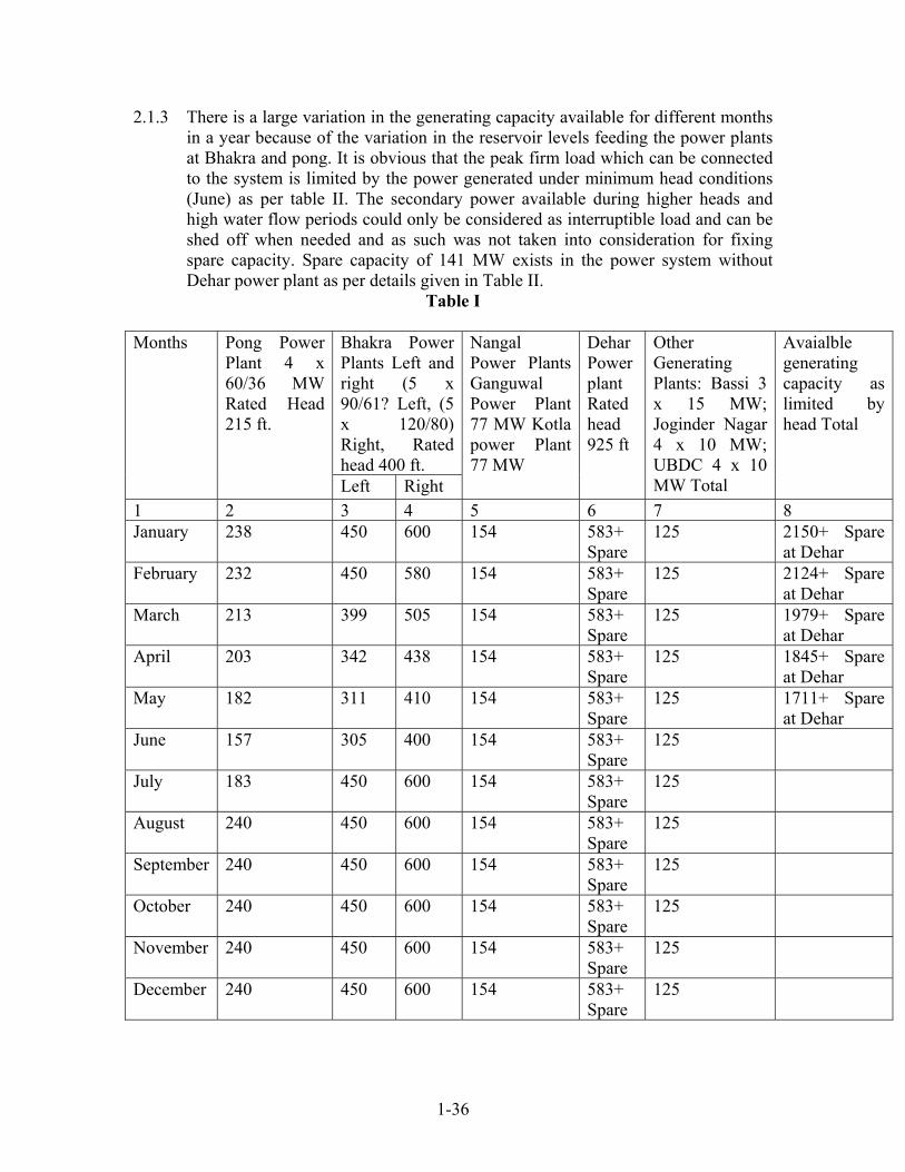
2.1.3 There is a large variation in the generating capacity available for different months in a year because of the variation in the reservoir levels feeding the power plants at Bhakra and pong. It is obvious that the peak firm load which can be connected to the system is limited by the power generated under minimum head conditions (June) as per table II. The secondary power available during higher heads and high water flow periods could only be considered as interruptible load and can be shed off when needed and as such was not taken into consideration for fixing spare capacity. Spare capacity of 141 MW exists in the power system without Dehar power plant as per details given in Table II.

Table I

Bhakra Power Plants Left and right (5 x 90/61? Left, (5 x 120/80) Right, Rated head 400 ft.

Months Pong Power Plant 4 x 60/36 MW Rated Head 215 ft.

Left Right

Nangal Power Plants Ganguwal Power Plant 77 MW Kotla power Plant 77 MW

Dehar Power plant Rated head 925 ft

Other Generating Plants: Bassi 3 x 15 MW; Joginder Nagar 4 x 10 MW; UBDC 4 x 10 MW Total

Avaialble generating capacity as limited by head Total

1 2 3 4 5 6 7 8 January 238 450 600 154 583+

Spare 125 2150+ Spare

at Dehar February 232 450 580 154 583+

Spare 125 2124+ Spare

at Dehar March 213 399 505 154 583+

Spare 125 1979+ Spare

at Dehar April 203 342 438 154 583+

Spare 125 1845+ Spare

at Dehar May 182 311 410 154 583+

Spare 125 1711+ Spare

at Dehar June 157 305 400 154 583+

Spare 125

July 183 450 600 154 583+ Spare

125

August 240 450 600 154 583+ Spare

125

September 240 450 600 154 583+ Spare

125

October 240 450 600 154 583+ Spare

125

November 240 450 600 154 583+ Spare

125

December 240 450 600 154 583+ Spare

125

1-37

2.2 Load Characteristics 2.2.1 There is an appericiable seasonal variation of laod. The monthly peak load

expressed as percentage of maximum monthly load of June (capacity under minimum head conditions) is shown in Table III.

2.2.2 A curve showing difference between monthly peak and daily maximum demand expressd as a percentage of monthly maximum demand in May/June is shown in Figure 1.

2.3 Scheduled maintenance and Seasonal Variation in Unit Capacities 2.3.1 As previously mentioned in the hydro system of the Punjab Power grid, there are

the following two critical periods: Table II

Power Plant

Minimum head in ft.

Number of Units

Power generated in MW Spare generating capacity in MW

Bhakra Left

284 5 5x 61 = 305

Bhakra Right

284 5 4 x 80 = 320 2 x 24 + 1 x 29 = 77

1 x 80 = 80

Ganguwal - 3 Kotla - 3 2 x 24 + 1 x 29 = 77 Joginder Nagar

- 4 4 x 10 = 40

Bassi - 3 2 x 15 = 30 1 x 15 = 15 UBDC - 4 3 x 10 = 30 1 x 10 = 10 Pong 156 4 3 x 36 = 108 1 x 36 = 36 Dehar 4 = 583 Spare

Table III Month Maximum monthly load as

percentage of maximum load of June

System peak load in MW

January 95.5 1498 February 95.5 1498 March 95.5 1498 April 100 1570 May 100 1570 June 100 1570 July 95.5 1495 August 95.5 1498 September 109.5 1718 November 109.5 1718 December 109.5 1718

1-38

(i) The period of minimum generating capacity when the heads at Bhakra and pong

reservoirs will be minimum. This period lies in May and June. Maintenance and inspection of gates, gate guides, etc. for Bhakra plants may be required to be carried out in the month of June when the head is minimum. Capacity outage amounting to not more than 80 MW for a period of one month was assumed during the month of June (minimum head) for this purpose.

(ii) The period of low-water availability, i.e., about five months from December to April when water releases are low. During the above five months, however, the heads are high and lot of spare generating capacity is available. It was, therefore, obvious that planed maintenance and major overhauls could be

1-39

carried out during these months except the maintenance of penstock gate guides, etc., as mentioned above.

2.3.2 for determining the installed capacity required to be provided, we have to take

into consideration the period (i) above. 2.4 Transportation of Heavy Packages 2.4.1 The transport of heave packages to the site of power plant at Dehar is proposed by

barrages in Bhakra Lake from the rail head at that place. It was estimated that a single piece package weighing about 70 tons could be transported without much difficulty.

2.4.2 In the high head Dehar power plant it was considered that a transformer section shall constitute the heaviest single piece package for the purpose of transport. A three phase transformer of even 106 MW size was estimated to weigh much more than 70 tons and as such cannot be transported without making special transport arrangements or by resorting to site assembling.

2.4.3 Single Phase transformer units are accordingly tentatively proposed for this powerhouse and were indicated to be within the transportable limits available at site.

2.5 Miscellaneous Consideration – Physical Layout, Part Load Operation, etc. 2.5.1 It was evident that for a power system with Dehar power plant of maximum

working capacity of 583 MW, the studies should be carried out with the number of units of different tentative sizes varying from 6 to 4. More than 6 units of smaller size were considered to be too small to be economical, while less than 4 units of over 200 MW size were rejected from considerati9ons of part load operation, possible manufacturing difficulties, costlier transport arrangement and obviously larger spare capacities required. The layout of the power plant envisages 2 units on a common penstock header. Rough studies indicated that five units will not be economical and detailed studies for this case were also not carried out.

2.5.2 The capacity of the unit in each alternative considered was such that the system

load be served with the same degree of reliability, the extra spare capacity required was incorporated into the units at Dehar.

3. Spare Generating Capacity 3.0 The plant peak capacity required in the system in any month must be equal to the

sum of the monthly peak load, overhauling requirements and the capacity required for forced outages. The capacity required for forced outages is a function of the unit size and has accordingly an important bearing on the economical unit size to be installed at Dehar power plant. Probability studies were carried out to find out the capacity required for forced outage and thereby determine the reserve capacity

1-40

required. These studies were carried out generally in accordance with Method 3 (interval between outages) of the Americal Institute of Electrical Engineers Sub Committee Report (1) for the following conditions.

3.0.1 Power system with Dehar power plant of peak capacity 583 MW – The

following basic approach was developed to determine the reserve capacity required in the system.

(i) Determination by probability methods, the expected frequency and duration of

forced outage of generating capacity in power system for the post Dehar period for different unit sizes at Dehar.

(ii) Scheduling all planned maintenance during high head periods when increased capacities are available.

(iii) Evaluation of the reserve capacity on the basis of the estimated 12 monthly peak load in a given year instead of the yearly maximum demands only.

(iv) Determination of monthly peaking factor to take into account the effect of variations in week day daily peak loads within each month on the required installed reserve.

(v) Evaluation of the help during emergencies from interconnections (with say Delhi and U.P. Grids) and from dropping of interruptible load and thus reduction of installed reserve accordingly.

3.1 Expectation Of Forced Outage By Probability Methods 3.1.1 Expectation of forced outages were calculated by probability methods which gave

results in terms of frequency, interval and average duration of outages. The mathematical steps involved in making these calculations have been explained in Appendix – III of the A.I.E.E. Committee Report. (1)

3.1.2 Forced outage rate of hydro electric units adopted was taken from the large

compilation of this data by North West Pool of America (2) on 387 hydroelectric generators of all capacities. An earlier collection of this data was made by A.I.E.E. sub committee in 1949 (3). Attempts were made to compile the figures of actual outage rates as per available data on Shannan, Ganguwal, Kotla and Bhakra power plants, but due to incomplete data for the purpose much lower figures for outage rates were obtained. The outage rate actually adopted are given in Table IV.

3.1.3 The forced outage rate derived above is predicated on machine exposure. Since

the results of probability calculations were desired on a full time basis including scheduled maintenance time, the outage rate applicable to all machines is :

P = 22.64

11128882

22.64

+

×

= 0.0065848

1-41

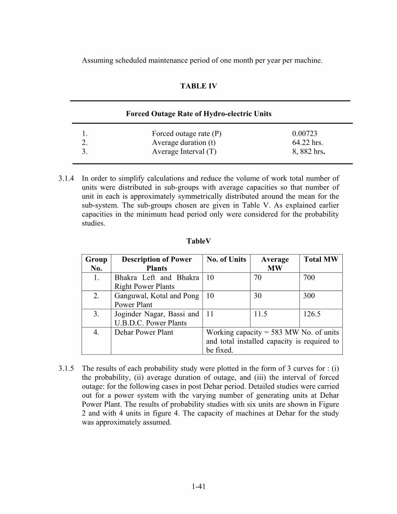
Assuming scheduled maintenance period of one month per year per machine.

TABLE IV

Forced Outage Rate of Hydro-electric Units

1. Forced outage rate (P) 0.00723 2. Average duration (t) 64.22 hrs. 3. Average Interval (T) 8, 882 hrs.

3.1.4 In order to simplify calculations and reduce the volume of work total number of

units were distributed in sub-groups with average capacities so that number of unit in each is approximately symmetrically distributed around the mean for the sub-system. The sub-groups chosen are given in Table V. As explained earlier capacities in the minimum head period only were considered for the probability studies.

TableV

Group

No. Description of Power

Plants No. of Units Average

MW Total MW

1. Bhakra Left and Bhakra Right Power Plants

10 70 700

2. Ganguwal, Kotal and Pong Power Plant

10 30 300

3. Joginder Nagar, Bassi and U.B.D.C. Power Plants

11 11.5 126.5

4. Dehar Power Plant Working capacity = 583 MW No. of units and total installed capacity is required to be fixed.

3.1.5 The results of each probability study were plotted in the form of 3 curves for : (i)

the probability, (ii) average duration of outage, and (iii) the interval of forced outage: for the following cases in post Dehar period. Detailed studies were carried out for a power system with the varying number of generating units at Dehar Power Plant. The results of probability studies with six units are shown in Figure 2 and with 4 units in figure 4. The capacity of machines at Dehar for the study was approximately assumed.

1-42

3.2 Spare Generating Capacity For Forced Outages 3.2.1 The maximum peak load that can be met and the available plant generating

capacity (with 4 units of 165 MW at Dehar) during different months in a year have been plotted in Figure 3. A perusal of this curve would reveal that the condition of minimum available plant capacity lasts for about one month in a year. For the rest of the period, due to higher heads, more plant capacity is available. Consequently the spare plant capacity required is to be of consequence for one month in a year for any forced or unforeseen plant outages. Further as already mentioned, a capacity of 80 MW may be required to e out for maintenance, etc., during this month. During the remaining periods of the year, the capacities available are higher and in months when more water flow is available, secondary power (considered interruptible load) could also be obtained from the power plants. A probability of once in 0.8 year forced outage indicated on the probability curves in figures 2 to 4 would actually mean a probability of once in about ten years forced outage (i.e., once in 8 x 12) because of possibility of the forced outage being of consequence only in the particular one month, i.e., (June) of the year. Provision against a probable forced outage occurring once in 10 years was considered quite sufficient and was assumed in the study for calculating reserve capacities. Accordingly these curves would indicate that for an outage of once in 1 year interval (i.e., an interval of 0.8 years on the curve) the following spare capacities are required in the grid for force outage in the month of June:

Outage Mag. Outage Duration

Power System with Dehar Power 144 MW 0.0038 years (1.4 days) Plant (6 Unites) Power System with Dehar Power 170 MW 0.0038 (1.4 days) Plant (4 Unites)

It is, therefore, obvious that spare capacity of 141 MW available in the power system without Dehar power plant (mentioned earlier) is quite sufficient. Further the spare capacities required to be provided for forced outage in the other months of the year for once in 10 years interval would be available because of higher heads.

3.3 Monthly Peaking Factor 3.3.1 To take into account the fact that a major forced outage is not likely to occur on

the day of the monthly peak, a monthly peaking factor was taken into consideration. The average duration of a forced outage is of the order of a day only, so if we provide for 90 percent of the days and leave the 10 percent, the probability of once in 10 years will be virtually once in 100 years. The curve in

1-43

Figure 1 shows that on 90 percent days the peak demand is about 2 percent value of that would be 32 MW. The total reserve in the system could, therefore, be reasonably reduced by 32 MW. As such actual reserve required for meeting forced outage is 144 – 32 -= 112 MW for power system with 6 units at Dehar and 170 – 32 = 138 MW for power system with 4 units at Dehar

3.4 Spare Generating Capacity Required at Dehar Power Plant 3.4.1 Spare generating capacity required in the system for meeting forced outages and

planned maintenance with Dehar power plant of 6 units and 4 units is as below:

MW19280112.}units6ofPlantPowerDeharwithSystemPower =+ MW21880138.}units4ofPlantPowerDeharwithSystemPower =+

Where 112 MW and 138 MW is the capacity required for forced outages for 6 and 4 units respectively, as worked out earlier and 80 MW is the capacity outage required for scheduled maintenance in low head period which is critical for generating capacity purpose.

1-44

1-45

Where 112 MW and 138 MW is the capacity required for forced outages for 6 and 4 units respectively, as worked out earlier and 80 MW is the capacity outage required for scheduled maintenance in low head period which is critical for generating capacity purpose.

3.4.2 Spare generating capacity equal to 141 MW is already available in the system

without Dehar Power Plant. Therefore, spare capacity required to be provided at Dehar power plant for 6 units is (192-141) 51 MW and for four untis (218-141) 77 MW.

3.5 Effects of Interconnection 3.51 It is evident that the capacity benefits resulting from future interconnection of

power grids of adjoining states could be evaluated and deducted from reserve needed to take care of forced outages. It was considered that this capacity benefit should provide a safe margin over the spare capacity figures worked out above. In the expanding Punjab power grid there would be scope for adjustment in the capacities of new power plants, so as to fully exploit the benefits of the already constructed power plants.

1-46

4. Size of Units 4.1 The maximum working capacity of the power plant being 583 MW it was evident

that a total installed capacity of 634 MW (583+51) would be required if 6 units are installed and 660 MW (583 + 77) would be required if 4 units are installed. The possible sizes accordingly assumed in the study worked out to: (a) 6 units of 106 MW each. (b) 4 units of 165 MW each

4.2 Four units of 165 MW each were selected for installation because of the following

considerations: (i) Substantial economies in the cost of equipment and civil structures are obtained

by the installation of lesser number of bigger size units in this high head plant. (ii) The system spare capacity with unit isze of 165 MW is not very much increased. (iii) The units of 165 MW size are within the manufacturing range available in the

country and can be transported to power plant site with the arrangements proposed.

(iv) Part load operation of the units in the grid is not liable to present any difficulty. 5. Conclusion

In view of the studies carried out is was apparent that four generating units 165 MW each be installed at Dehar power plant in the first stage so as to affect large economies in the cost of equipment and structure.

6. References

i) “Application of Probability Methods to Generating Capacity Problems”. AIEE Committee Report, AIEE Transactions February, 1961.

ii) Hilton, N., Brown III, Laurance, A. Beam, Alfred R. Capref: “Forced Generation Outage Investigations for the North-West Power Pool”. AIEE Transactions, October 1960.

iii) “Outage Rates Steam Turbines and Boilers and of Hydro Units”. AIEE Committee report, AIEE Transactions 1949, vol. 68, part I.