For a mean Standard deviation changes to standard error now that we are dealing with a sampling...
50
-
Upload
kory-phillips -
Category
Documents
-
view
221 -
download
1
Transcript of For a mean Standard deviation changes to standard error now that we are dealing with a sampling...
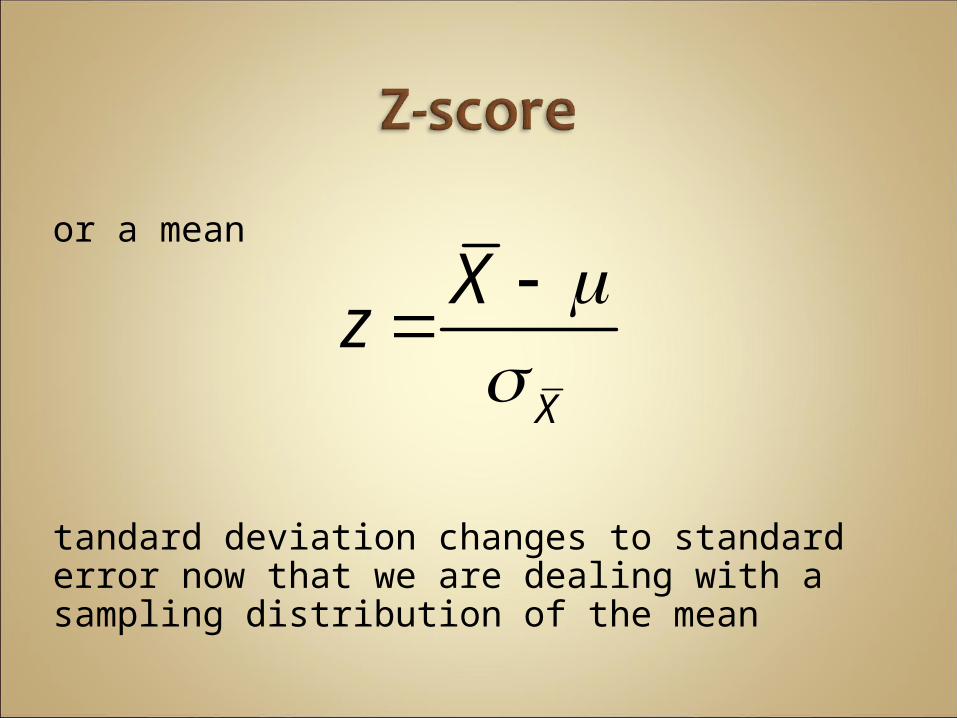
For a mean
Standard deviation changes to standard error now that we are dealing with a sampling distribution of the mean
X
Xz
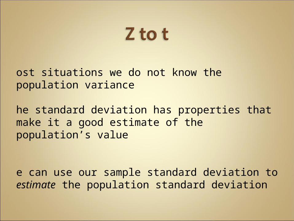
Most situations we do not know the population variance
The standard deviation has properties that make it a good estimate of the population’s value
We can use our sample standard deviation to estimate the population standard deviation
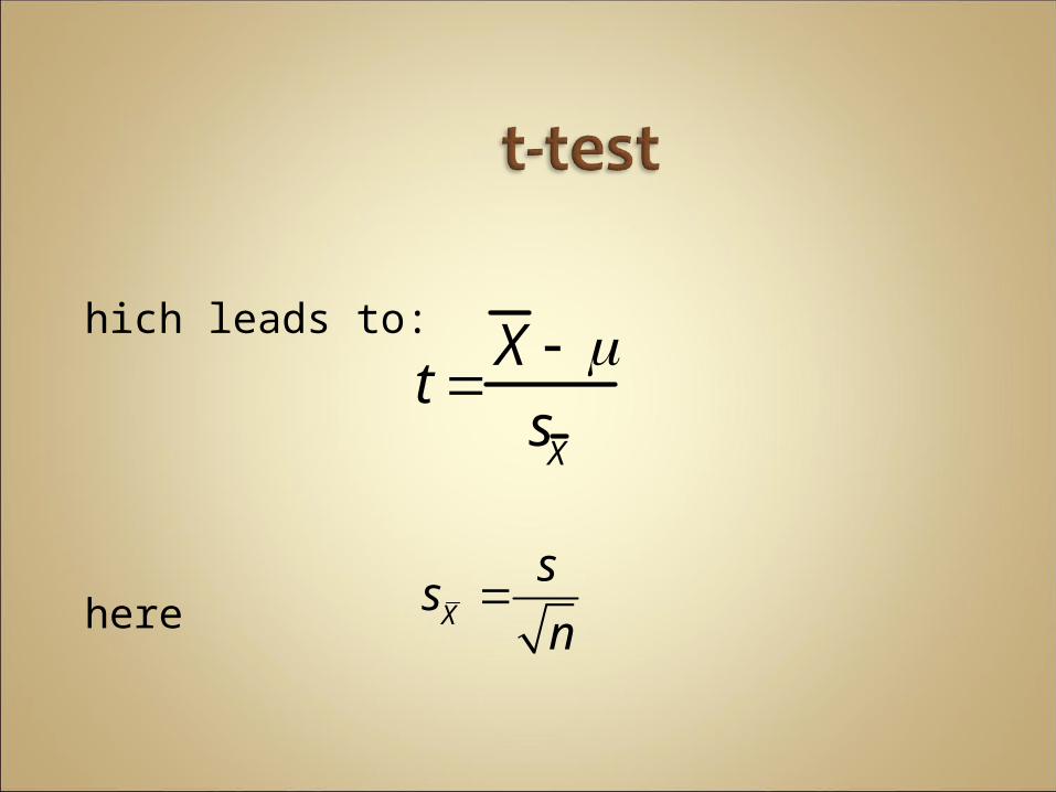
Which leads to:
Where
t X
sX
X
ss
n

Previously compared sample mean to a known population mean
Now want to compare two samples
Null hypothesis: the mean of the population of scores from which one set of data is drawn is equal to the mean of the population of the second data set
H0: 1=2 or 1 - 2 = 0

Usually we do not know population variance (standard deviation)
Again use sample to estimate it
Result is distributed as t (rather than z)
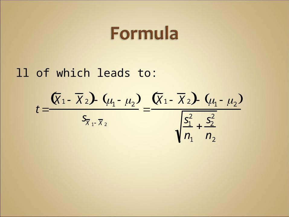
All of which leads to:
t X1 X 2 1 2
sX 1 X 2
X1 X 2 1 2
s12
n1
s22
n2
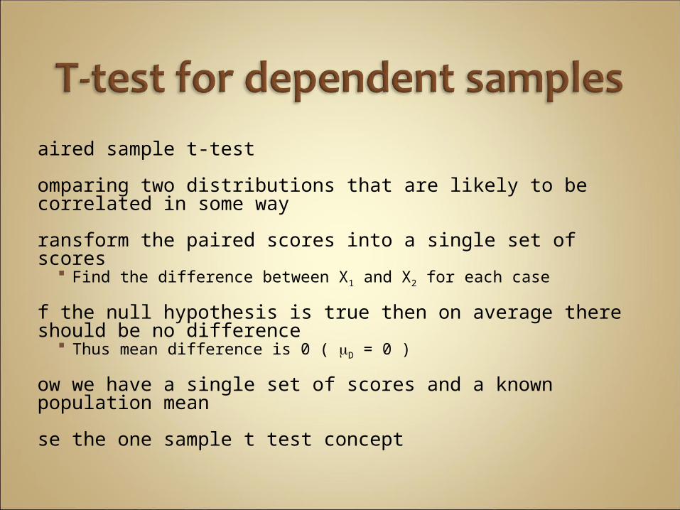
Paired sample t-test
Comparing two distributions that are likely to be correlated in some way
Transform the paired scores into a single set of scores
Find the difference between X1 and X2 for each caseI
f the null hypothesis is true then on average there should be no difference
Thus mean difference is 0 ( D = 0 )N
ow we have a single set of scores and a known population mean
Use the one sample t test concept
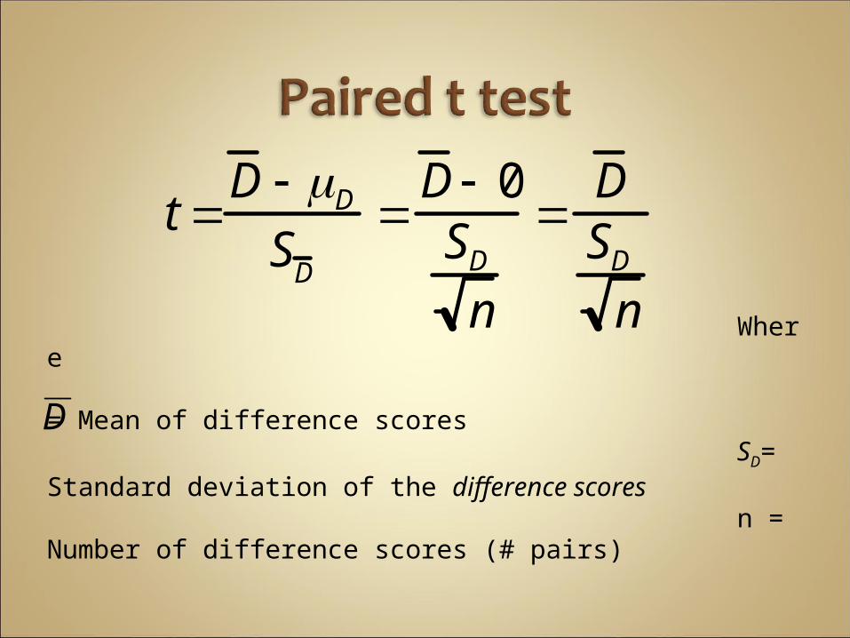
Where
= Mean of difference scores
SD
= Standard deviation of the difference scoresn
= Number of difference scores (# pairs)
t D D
SD
D 0
SD
n
DSD
n
D

What if your question regards equivalence rather than a difference between scores?
Example: want to know if two counseling approaches are similarly efficacious
Just do a t-test, and if non-significant conclude they are the same
Wrong! It would be logically incorrect.
Can you think of why?
Recall confidence intervals
The mean or difference between means is a point estimate
We should also desire an interval estimate reflective of the variability and uncertainty of our measurement seen in the data
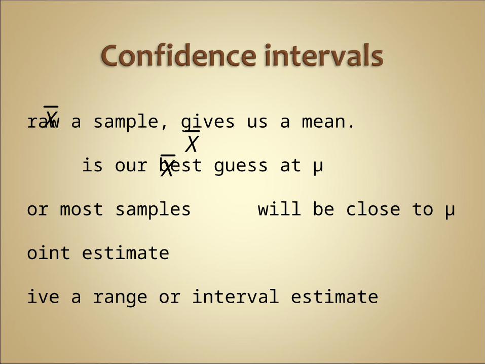
Draw a sample, gives us a mean.
is our best guess at µ
For most samples will be close to µ
Point estimate
Give a range or interval estimate
X
X
X
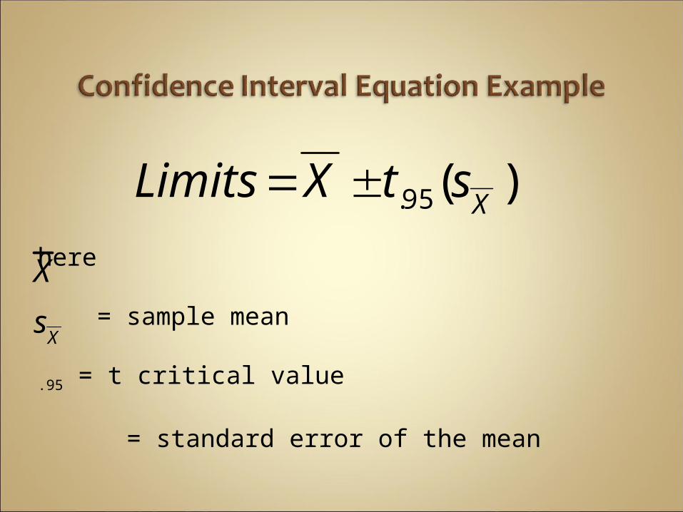
Where
= sample mean
t.95 = t critical value
= standard error of the mean
)(95. XstXLimits
Xs
X
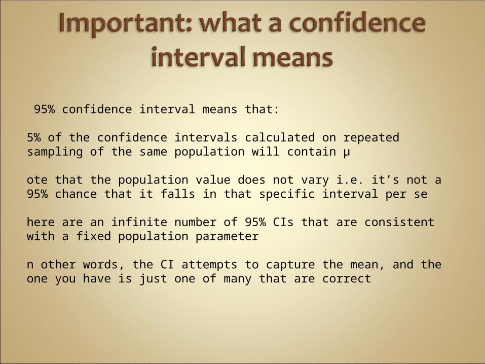
A 95% confidence interval means that:
95% of the confidence intervals calculated on repeated sampling of the same population will contain µ
Note that the population value does not vary i.e. it’s not a 95% chance that it falls in that specific interval per se
There are an infinite number of 95% CIs that are consistent with a fixed population parameter
In other words, the CI attempts to capture the mean, and the one you have is just one of many that are correct
http://www.ruf.rice.edu/~lane/stat_sim/conf_interval/index.html
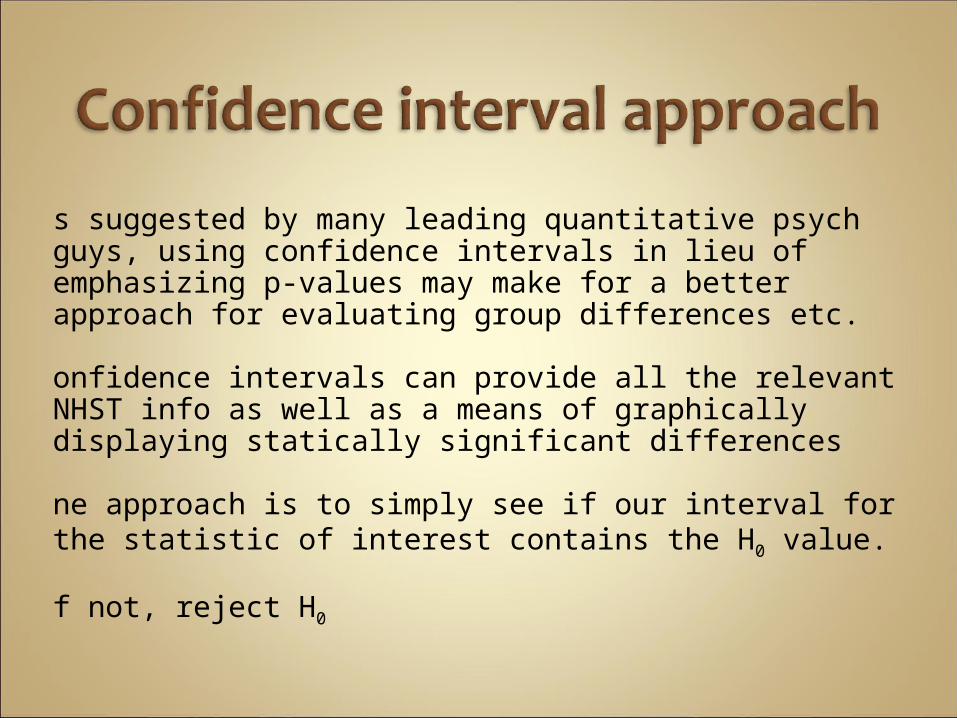
As suggested by many leading quantitative psych guys, using confidence intervals in lieu of emphasizing p-values may make for a better approach for evaluating group differences etc.
Confidence intervals can provide all the relevant NHST info as well as a means of graphically displaying statically significant differences
One approach is to simply see if our interval for the statistic of interest contains the H0 value.
If not, reject H0
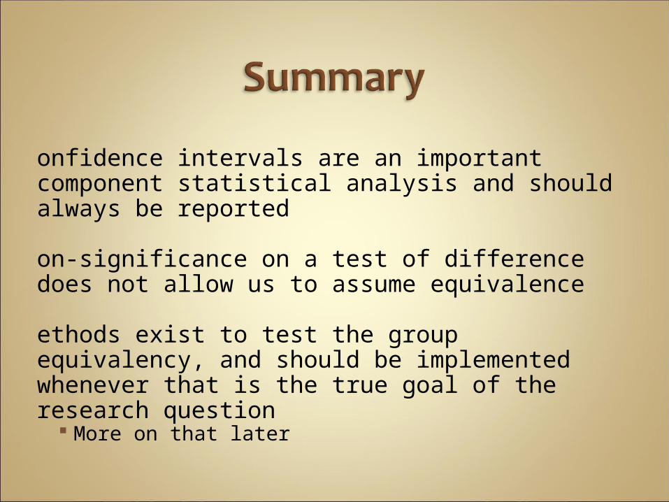
Confidence intervals are an important component statistical analysis and should always be reported
Non-significance on a test of difference does not allow us to assume equivalence
Methods exist to test the group equivalency, and should be implemented whenever that is the true goal of the research question
More on that later

Most popular analysis in psychology
Ease of implementation Allows for analysis of several groups at once Allows analysis of interactions of multiple
independent variables.

2..( )jn X X
2..( )ijX X
2( )ij jX X
S S treatm ent S S error
S S total
S S Between groups S S with in groups
S S total

If the assumptions of the test are not met we may have problems in its interpretation
Assumptions
Independence of observations Normally distributed variables of measure Homogeneity of Variance
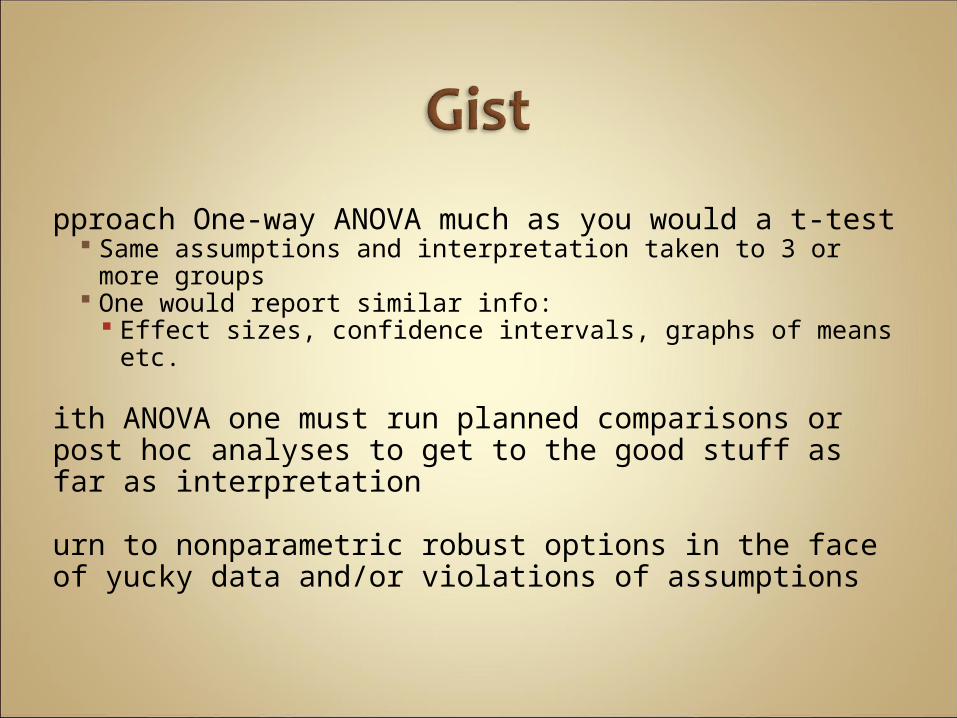
Approach One-way ANOVA much as you would a t-test
Same assumptions and interpretation taken to 3 or more groups
One would report similar info: Effect sizes, confidence intervals, graphs of means etc.
With ANOVA one must run planned comparisons or post hoc analyses to get to the good stuff as far as interpretation
Turn to nonparametric robust options in the face of yucky data and/or violations of assumptions
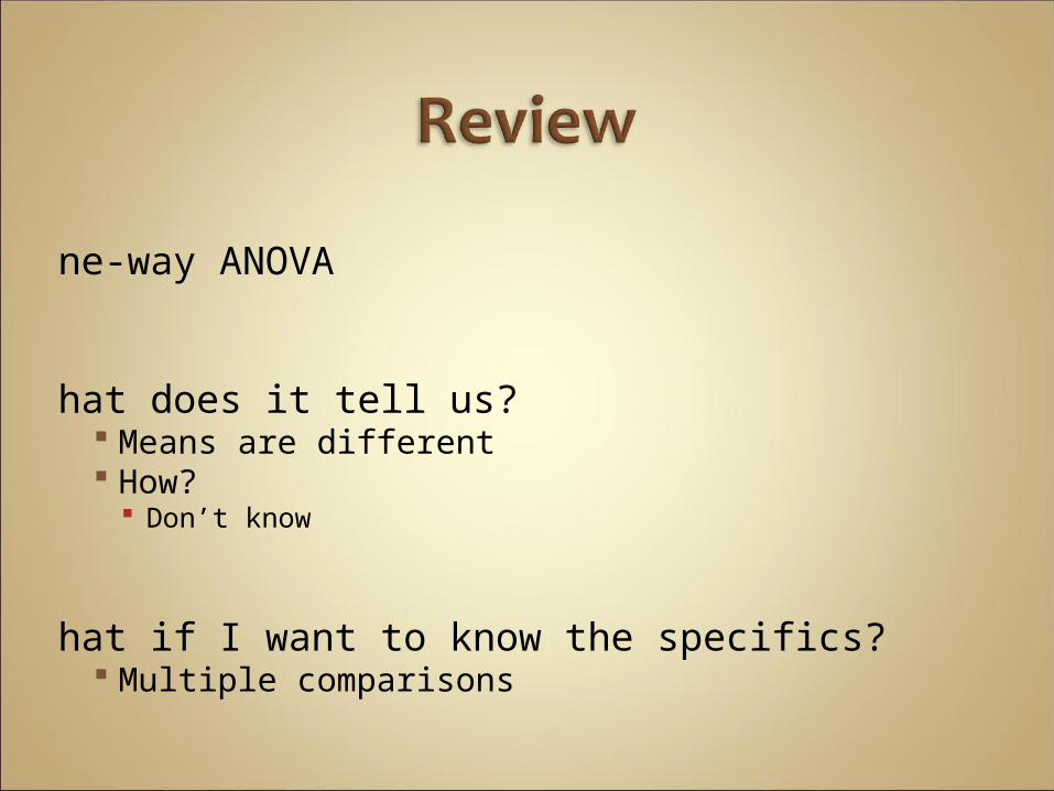
One-way ANOVA
What does it tell us?
Means are different How?
Don’t know
What if I want to know the specifics?
Multiple comparisons

We can do multiple comparisons with a correction for type I error or planned contrasts to test the differences we expect based on theory
A prior vs. Post hoc
Before or after the factA
priori Do you have an expectation of the results based on
theory? A priori Few comparisons More statistically powerful
Post hoc
Look at all comparisons while maintaining type I error rate

Do we need an omnibus F test first?
Current thinking is no Most multiple comparison procedures are
maintain type I error rates without regard to omnibus F results
Multivariate analogy We do multivariate and then interpret in terms of uni
anovas Begs the question of why the multivariate approach was
taken in the first place

Some are better than others
However which are better may depend on situation
Try alternatives, but if one is suited specifically for your situation use it.
Some suggestions
Assumptions met: Tukey’s or REWQ of the traditional options, FDR for more power
Unequal n: Gabriel’s or Hochberg (latter if large differences) Unequal variances: Games-Howell
More later
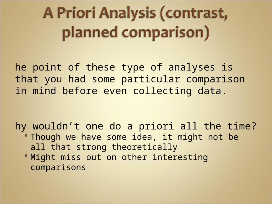
The point of these type of analyses is that you had some particular comparison in mind before even collecting data.
Why wouldn’t one do a priori all the time?
Though we have some idea, it might not be all that strong theoretically
Might miss out on other interesting comparisons

Let theory guide which comparisons you look at
Have a priori contrasts in mind whenever possibleT
est only comparisons truly of interestU
se more recent methods for post hocs for more statistical power
Factorial Anova
Repeated Measures
Mixed
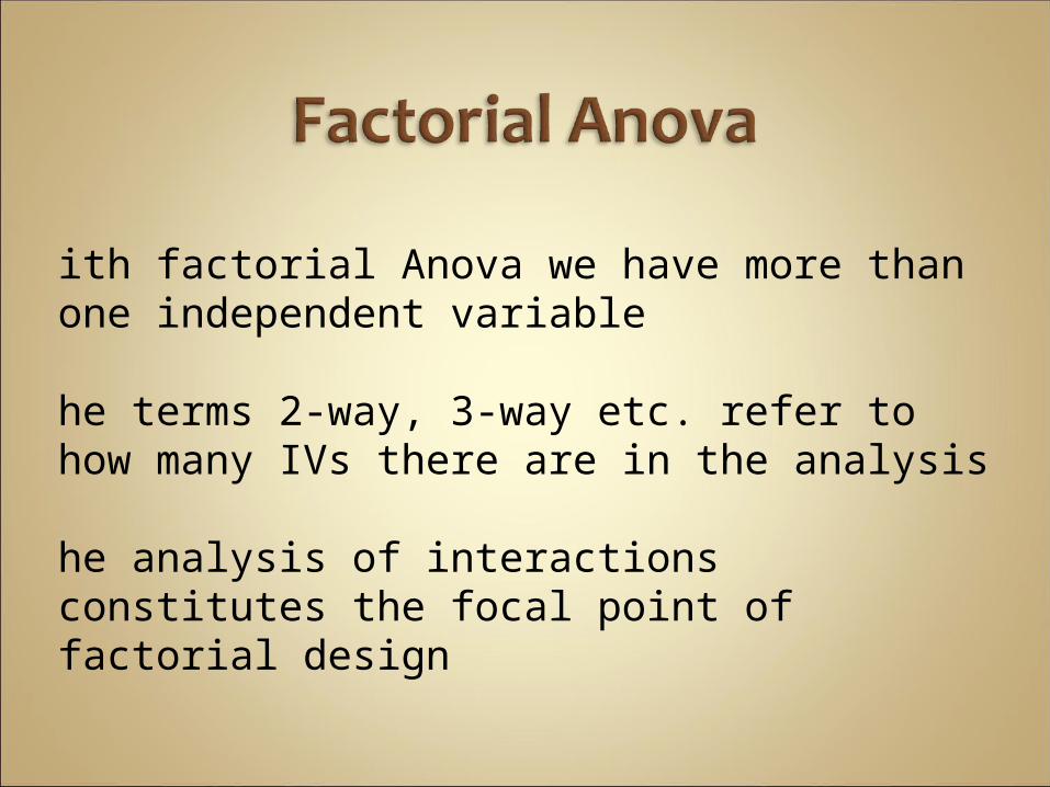
With factorial Anova we have more than one independent variable
The terms 2-way, 3-way etc. refer to how many IVs there are in the analysis
The analysis of interactions constitutes the focal point of factorial design
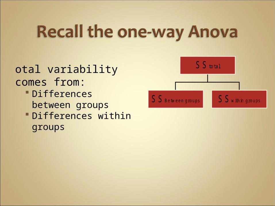
Total variability comes from:
Differences between groups
Differences within groups
S S Between groups S S with in groups
S S total
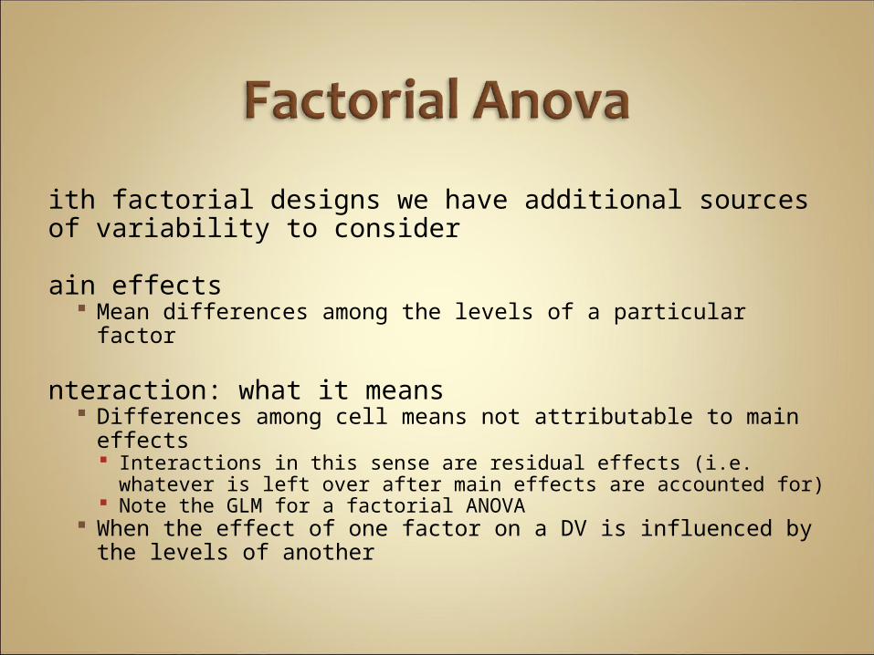
With factorial designs we have additional sources of variability to consider
Main effects
Mean differences among the levels of a particular factorI
nteraction: what it means Differences among cell means not attributable to main
effects Interactions in this sense are residual effects (i.e. whatever is
left over after main effects are accounted for) Note the GLM for a factorial ANOVA
When the effect of one factor on a DV is influenced by the levels of another

Total variability
Between-treatments var. Within-treatments var.
Factor Avariability
Factor Bvariability
Interactionvariability
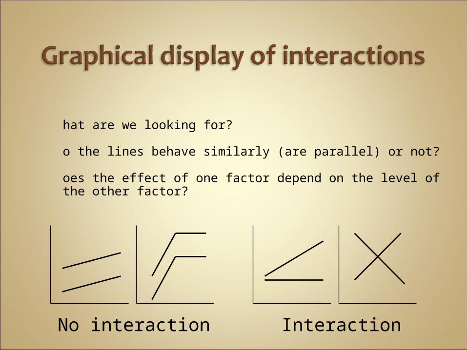
What are we looking for?
Do the lines behave similarly (are parallel) or not?
Does the effect of one factor depend on the level of the other factor?
No interaction Interaction

Note that with a significant interaction, the main effects are understood only in terms of that interaction
In other words, they cannot stand alone as an explanation and must be qualified by the interaction’s interpretation
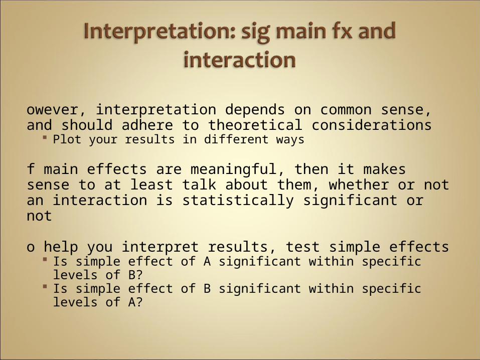
However, interpretation depends on common sense, and should adhere to theoretical considerations
Plot your results in different waysI
f main effects are meaningful, then it makes sense to at least talk about them, whether or not an interaction is statistically significant or not
To help you interpret results, test simple effects
Is simple effect of A significant within specific levels of B?
Is simple effect of B significant within specific levels of A?

Analysis of the effects of one factor at one level of the other factor
Example:
Levels of A1-3 at B1 and A1-3 at B2 N
ote that the simple effect represents a partitioning of SSmain effect and SSinteraction
Not just a breakdown of the interaction!
1.00 2.00
VAR00001
0
1
2
3
4
Mea
n V
AR
000
02
VAR00003
1.00
2.00
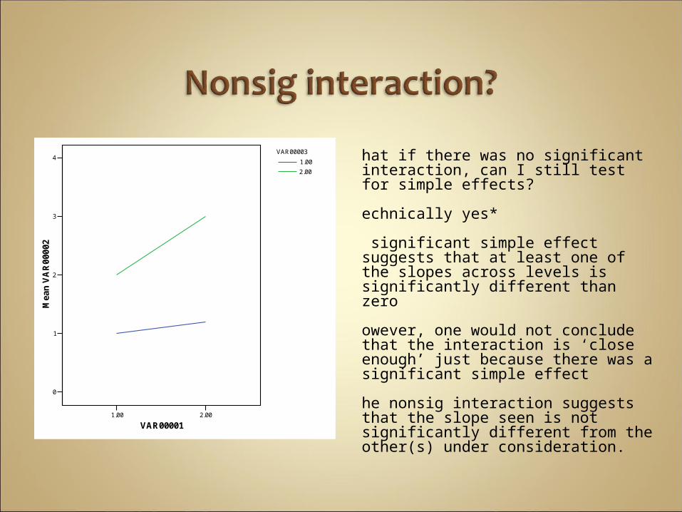
What if there was no significant interaction, can I still test for simple effects?
Technically yes*
A significant simple effect suggests that at least one of the slopes across levels is significantly different than zero
However, one would not conclude that the interaction is ‘close enough’ just because there was a significant simple effect
The nonsig interaction suggests that the slope seen is not significantly different from the other(s) under consideration.
Instead of having one score per subject, experiments are frequently conducted in which multiple scores are gathered for each case
Repeated Measures or Within-subjects design
Advantages
Design – nonsystematic variance (i.e. error, that not under experimental control) is reduced Take out variance due to individual differences
Efficiency – fewer subjects are required More sensitivity/power
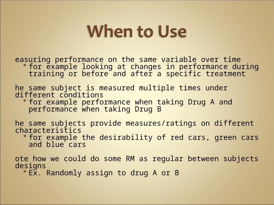
Measuring performance on the same variable over time
for example looking at changes in performance during training or before and after a specific treatment
The same subject is measured multiple times under different conditions
for example performance when taking Drug A and performance when taking Drug B
The same subjects provide measures/ratings on different characteristics
for example the desirability of red cars, green cars and blue cars
Note how we could do some RM as regular between subjects designs
Ex. Randomly assign to drug A or B
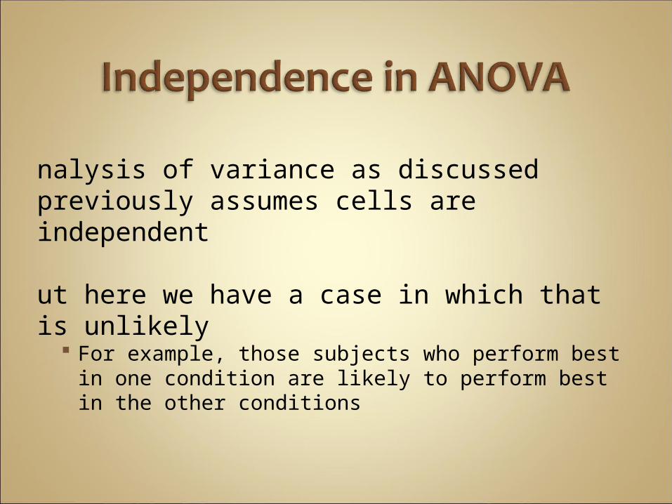
Analysis of variance as discussed previously assumes cells are independent
But here we have a case in which that is unlikely
For example, those subjects who perform best in one condition are likely to perform best in the other conditions
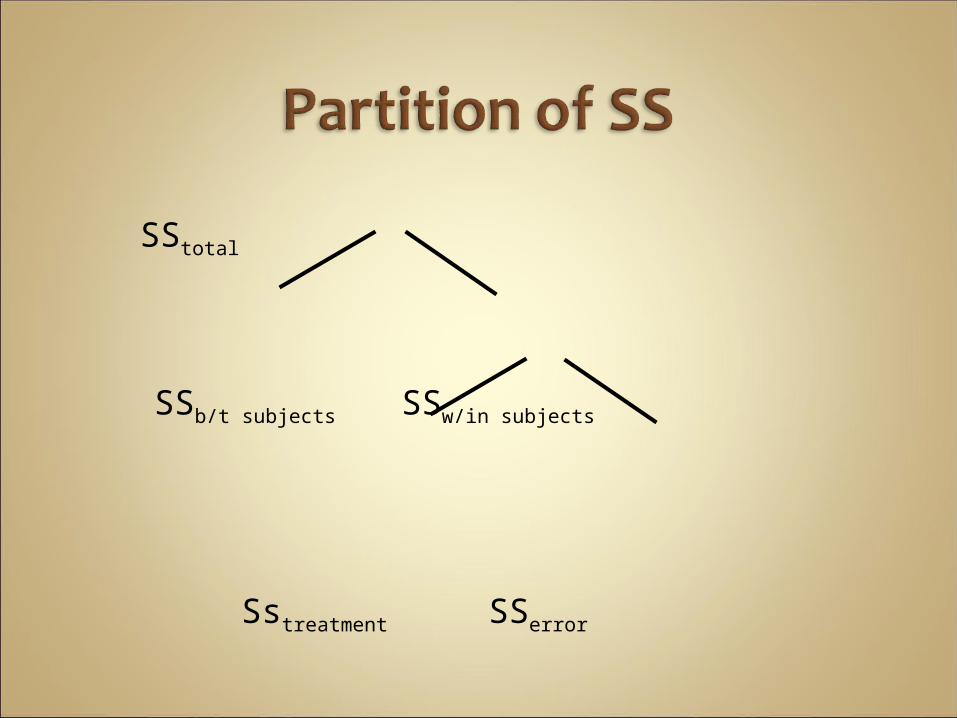
SStotal
SSb/t subjects SSw/in subjects
Sstreatment SSerror
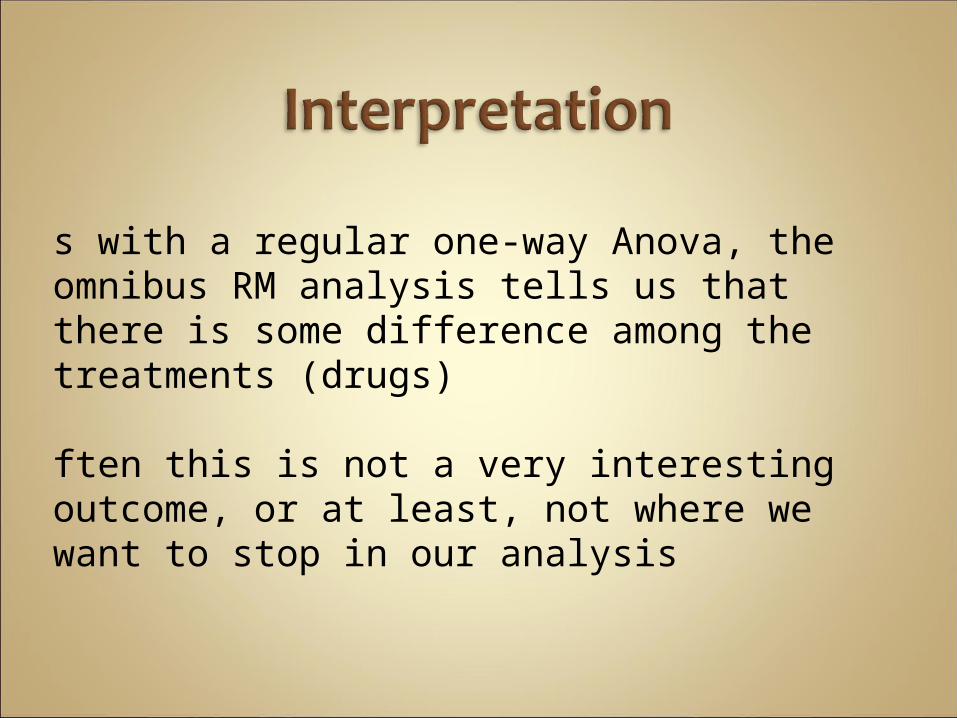
As with a regular one-way Anova, the omnibus RM analysis tells us that there is some difference among the treatments (drugs)
Often this is not a very interesting outcome, or at least, not where we want to stop in our analysis
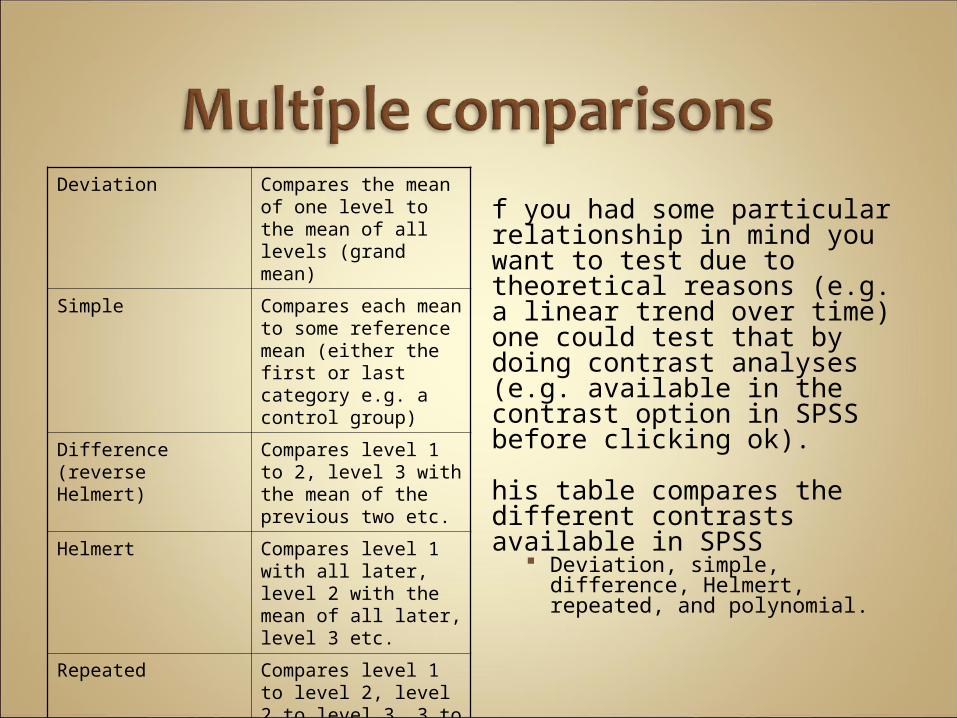
Deviation Compares the mean of one level to the mean of all levels (grand mean)
Simple Compares each mean to some reference mean (either the first or last category e.g. a control group)
Difference (reverse Helmert)
Compares level 1 to 2, level 3 with the mean of the previous two etc.
Helmert Compares level 1 with all later, level 2 with the mean of all later, level 3 etc.
Repeated Compares level 1 to level 2, level 2 to level 3, 3 to 4 and so on
Polynomial Tests for trends (e.g. linear) across levels
If you had some particular relationship in mind you want to test due to theoretical reasons (e.g. a linear trend over time) one could test that by doing contrast analyses (e.g. available in the contrast option in SPSS before clicking ok).
This table compares the different contrasts available in SPSS
Deviation, simple, difference, Helmert, repeated, and polynomial.
Observations may covary, but the degree of covariance must remain the same
If covariances are heterogeneous, the error term will generally be an underestimate and F tests will be positively biased
Such circumstances may arise due to carry-over effects, practice effects, fatigue and sensitization

Suppose the factor TIME had 3 levels – before, after and follow-up
RM ANOVA assumes that the 3 correlations
r ( Before-After ) r ( Before-Follow up ) r ( After-Follow up )
are all about the same in size
A x (B x S)
At least one between, one within subjects factor
Each level of factor A contains a different group of randomly assigned subjects.
On the other hand, each level of factor B at any given level of factor A contains the same subjects

Partitioning the variance is done as for a standard ANOVA
Within subjects error term used for repeated measures
What error term do we use for the interaction of the two factors?
Again we adopt the basic principle we have followed previously in looking for effects. We want to separate between treatment effects and error
A part due to the manipulation of a variable, the treatment part (treatment effects)
A second part due to all other uncontrolled sources of variability (error)
The deviation associated with the error can be divided into two different components:
Between Subjects Error Estimates the extent to which chance factors are responsible
for any differences among the different levels of the between subjects factor.
Within Subjects Error Estimates the extent to which chance factors are responsible
for any differences observed within the same subject
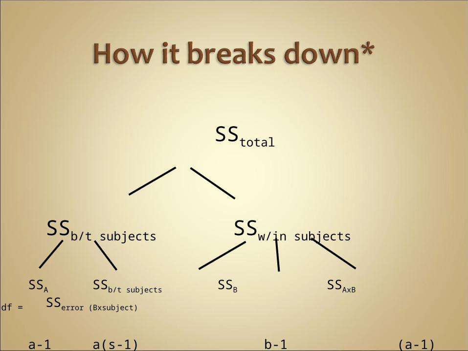
SStotal
SSb/t subjects SSw/in subjects
SSA SSb/t subjects SSB SSAxB SSerror
(Bxsubject)
a-1 a(s-1) b-1 (a-1)(b-1) a(b-1)(s-1)
df =
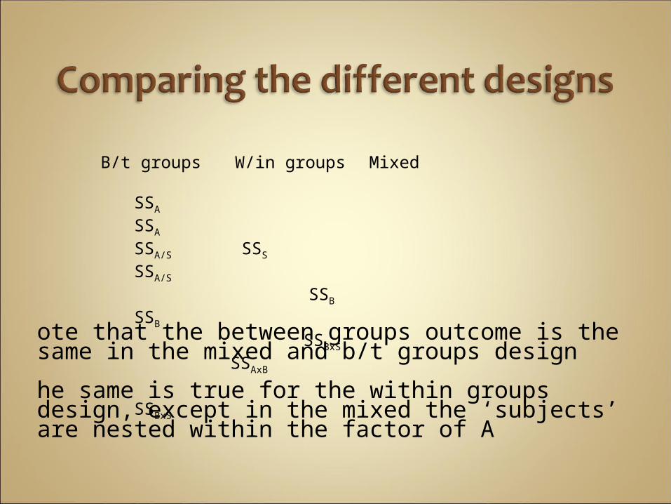
Note that the between groups outcome is the same in the mixed and b/t groups design
The same is true for the within groups design, except in the mixed the ‘subjects’ are nested within the factor of A
B/t groups W/in groups Mixed
SSA SSA
SSA/S SSS SSA/S
SSB SSB
SSBxS
SSAxB
SSBxS

The SSb/t subjects reflects the deviation of subjects from the grand mean while the SSw/in reflects their deviation from their own mean
The mixed design is the conjunction of a randomized single factor experiment and a single factor experiment with repeated measures
Though this can be extended to have more than one b/t groups or repeated factor
![[XLS]people.highline.edu · Web view=ROUNDUP(B26,0) Amount Mean sigma Pop standard deviation Standard Error (Standard Deviation of Distribution of Xbar) Confidence Level = or Confidence](https://static.fdocuments.in/doc/165x107/5b01a7487f8b9a84338e75aa/xls-viewroundupb260-amount-mean-sigma-pop-standard-deviation-standard-error.jpg)