Food and Prices in India:

Impact of Rising Food Prices on Welfare

Nathalie Pons∗1

1Centre de Sciences Humaines (Delhi)

September 23, 2011

Abstract

The paper presents the impact of a simulated increase in food prices on the household’s wel-fare in India from the NSS Survey ”Consumer Expenditure” (Round 61st). It attemptsto understand which households are the most vulnerable to rising food prices. Demand

reactions and elasticities are computed from the Almost Ideal Demand System. Only demand istaking into account. The effect is computed assuming that the other influential parameters havenot changed.

This study shows that there are differential impacts on different categories of households. Ru-ral households are more vulnerable than urban households. In addition, the poorest householdsof both sectors are more penalized by rising food price than the richest households. The impactdepends also on the commodity which price has increased. Indeed, an increase in cereal pricesaffects more the households than the same increase in fruit price.

Keywords — Elasticity, Welfare, Inflation, AIDS, Compensating Variation, Unit Value, NSSData.

∗I am grateful to my tutor Basudeb Chaudhuri, director of the Centre de Sciences Humaines and Himanshu fortheir helpful comments. I thank a lot Mainak Mazumdar for his corrections. I thank Himanshu again for sharing someof the data that I have used in this paper. For any comments, please send me a message: pons.nathalie@gmail.com

1

Contents

1 Introduction 31.1 Context . . . . . . . . . . . . . . . . . . . . . . . . . . . . . . . . . . . . . . . . . . . 31.2 Review of the Literature . . . . . . . . . . . . . . . . . . . . . . . . . . . . . . . . . 4

2 Analytical Framework and Empirical Approach 62.1 Compensating Variation . . . . . . . . . . . . . . . . . . . . . . . . . . . . . . . . . 62.2 Demand System . . . . . . . . . . . . . . . . . . . . . . . . . . . . . . . . . . . . . . 62.3 Estimation . . . . . . . . . . . . . . . . . . . . . . . . . . . . . . . . . . . . . . . . . 72.4 Inflation Scenario . . . . . . . . . . . . . . . . . . . . . . . . . . . . . . . . . . . . . 8

3 Data 103.1 NSS Survey . . . . . . . . . . . . . . . . . . . . . . . . . . . . . . . . . . . . . . . . . 103.2 Treatment of Outliers and Missing Values . . . . . . . . . . . . . . . . . . . . . . . . 103.3 Consumption Pattern . . . . . . . . . . . . . . . . . . . . . . . . . . . . . . . . . . . 11

4 Demand Results 124.1 Taste and Demand Parameters . . . . . . . . . . . . . . . . . . . . . . . . . . . . . . 124.2 Elasticities . . . . . . . . . . . . . . . . . . . . . . . . . . . . . . . . . . . . . . . . . 13

5 Estimated Impact of Rising Food Prices on Welfare 155.1 Magnitude of the Impact and Demand Adjustment . . . . . . . . . . . . . . . . . . 155.2 Who Are the Most Vulnerable? . . . . . . . . . . . . . . . . . . . . . . . . . . . . . . 16

5.2.1 Poor vs. Rich . . . . . . . . . . . . . . . . . . . . . . . . . . . . . . . . . . . 165.2.2 Rural vs. Urban . . . . . . . . . . . . . . . . . . . . . . . . . . . . . . . . . . 175.2.3 SC/ST and Religion . . . . . . . . . . . . . . . . . . . . . . . . . . . . . . . . 185.2.4 Household composition . . . . . . . . . . . . . . . . . . . . . . . . . . . . . . 185.2.5 Governmental Program . . . . . . . . . . . . . . . . . . . . . . . . . . . . . . 195.2.6 State Disparities . . . . . . . . . . . . . . . . . . . . . . . . . . . . . . . . . . 20

5.3 The Four Inflation Scenarios . . . . . . . . . . . . . . . . . . . . . . . . . . . . . . . 21

6 Concluding Remarks 21

References 23

A Appendix 24

2

1. INTRODUCTION

1.1. Context

Last years are characterized in India by growth at historically unprecedented rates. Real percapita income has also grown rapidly; poverty has declined. However, inequalities have in-

creased.

Poor households don’t benefit from the positive effects of growth. Health and education relatedindicators have improved, but this progress has been unsatisfactory, even when compared to otherdeveloping countries. Huge inter-state disparities in health and education related indicators re-main. Growth picked out, but the level of rural poverty remains high (because of stagnation in theagricultural real wage and low access to public goods). For the poor households, in India, healthindicators are particularly dire. The private health sector as currently organized is unlikely toimprove the health and nutritional status of the poor household substantially. For education, thedirect cost, even for public schools and even ignoring the opportunity cost, is nearly prohibitive fora poor family1. Furthermore, Himanshu [14] noticed that from 1993 to 2004, the poor householdsdidn’t really benefit from a period of very low food price inflation to improve their welfare.

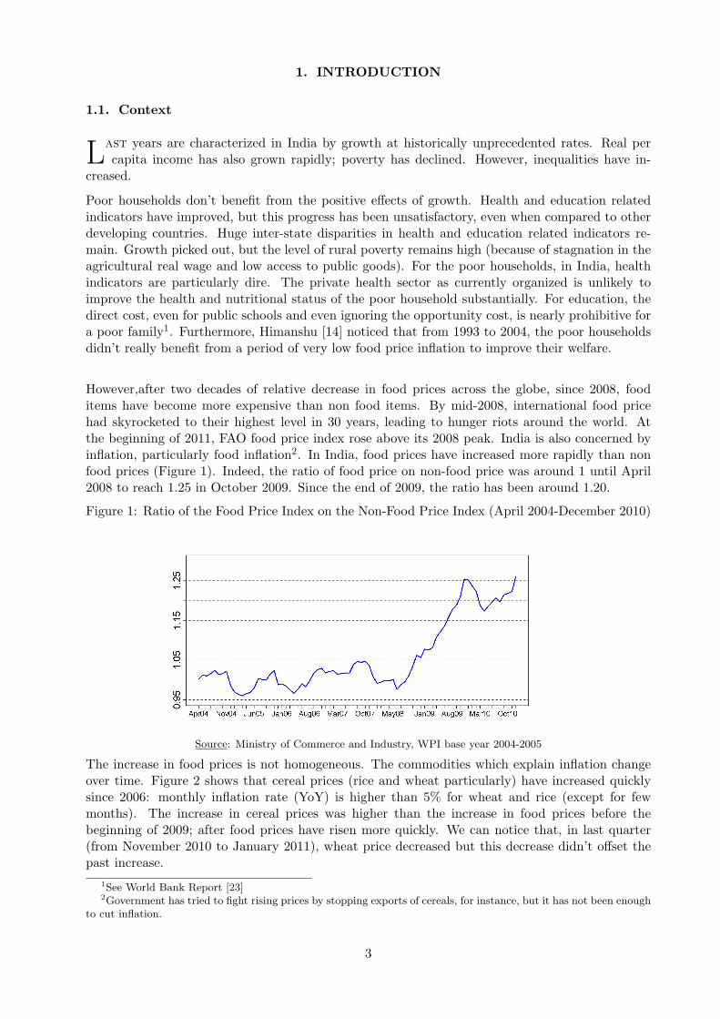
However,after two decades of relative decrease in food prices across the globe, since 2008, fooditems have become more expensive than non food items. By mid-2008, international food pricehad skyrocketed to their highest level in 30 years, leading to hunger riots around the world. Atthe beginning of 2011, FAO food price index rose above its 2008 peak. India is also concerned byinflation, particularly food inflation2. In India, food prices have increased more rapidly than nonfood prices (Figure 1). Indeed, the ratio of food price on non-food price was around 1 until April2008 to reach 1.25 in October 2009. Since the end of 2009, the ratio has been around 1.20.

Figure 1: Ratio of the Food Price Index on the Non-Food Price Index (April 2004-December 2010)

texteSource: Ministry of Commerce and Industry, WPI base year 2004-2005

The increase in food prices is not homogeneous. The commodities which explain inflation changeover time. Figure 2 shows that cereal prices (rice and wheat particularly) have increased quicklysince 2006: monthly inflation rate (YoY) is higher than 5% for wheat and rice (except for fewmonths). The increase in cereal prices was higher than the increase in food prices before thebeginning of 2009; after food prices have risen more quickly. We can notice that, in last quarter(from November 2010 to January 2011), wheat price decreased but this decrease didn’t offset thepast increase.

1See World Bank Report [23]2Government has tried to fight rising prices by stopping exports of cereals, for instance, but it has not been enough

to cut inflation.

3

Figure 2: Monthly Inflation Rate (YoY)

texteSource: Ministry of Commerce and Industry, WPI base year 2004-2005

It is well-known that people are adversely affected by rising food prices which limit their purchasingpower. In order to develop efficient policies to fight the negative impact of rising food prices, it isnecessary to know which households are the most vulnerable, how food inflation affects them andthe magnitude of the impact on welfare.

1.2. Review of the Literature

Anumber of papers examines the effect of food price change on the household’s welfare, in de-veloping countries. Many works are based on the compensating variation, which corresponds

to the difference between two values of the expenditure function. A first-order approximation ofrelative welfare variation is given by the sum, across commodities, of the product of price changeby the household’s net purchases of each good. Some authors, such as Deaton, use non-parametricvariant of this concept. However, the first-order approximation neglects the substitution effects.A second-order Taylor expansion of the expenditure function attempts to estimate the effects ofsubstitution on welfare variation. This work can be found, for example, in Minot and Goletti [17]or Ulimwengu and Ramadam [20]. Both papers focus on just one change price.

Minot and Goletti [17] investigated the potential effect of a liberalization of rice market in VietNam. One chapter of their paper was about the link between poverty and rice prices. In thischapter, both authors simulated a uniform increase in rice price by 10% and compute the effecton welfare and poverty derived from the compensating variation. They didn’t estimate themselvesprice elasticities: they used elasticities computed by other authors from time-series data. Theyfind that overall welfare impacts are generally large but differ considerably not only between urbanand rural areas, but also across different regions. Surprisingly, there is no effect on poverty becausea lot of households are net sellers. Moreover, they underline that ”the welfare effects of a pricechange are more positive when consumer and producer responses are incorporated. However, thedifferences between short- and long-term effects are small, around 0.1 percentage points, as a resultof the relatively inelastic demand and supply.” (Minot and Goletti, p. 64).

Ulimwengu and Ramadam [20] investigated the effect of a change in cereal price on Ugandan house-holds’ welfare. They insisted on the importance of including the supply side on the analysis in orderto obtain non-pessimistic results. They underlined also the importance of agricultural services andmarket access. They warned against policy response focusing on the demand because it would tendto favor consumers at the expense of producers.

More recent papers focus on the impact of the food price crisis in 2008 in order to estimate the

4

effect but also to characterize the most vulnerable households.

Zezza and al. [21] made an effort at differentiating the impact of an increase in food prices acrosspopulation subgroups. Their work was based on 11 Living Standard Measurement Surveys (LSMS).They computed a first-order approximation of welfare variation following an increase in the threemain tradable staple food prices of the country. Their aim was to understand the determinantsof price vulnerability. Expenditure level is certainly important, but limiting the focus to thatmisses a large part of the determinant of vulnerability. Agricultural assets and livelihood strategyhave to be looked. The gaps between poor and non-poor households, rural and urban householdsare highlighted. Their paper underlines also the differential effect of some variables across thecountries. Indeed, the share of irrigated land has sometimes a negative impact, and sometimes apositive, depending on the country.

Ferreira and al. [24] examined this impact of food price crisis in Brazil. Indeed, while general infla-tion rate is around 5.3% in 2007-2008, food price inflation peaked at over 18% in mid-2008. Theirapproach was based on a three market approach: expenditure (demand), income (supply) and wage(labor). However, they neglected substitution effects. The overall effect of the price increases wasto raise both extreme and moderate poverty. The poor either gain or lose less from higher pricesthan the middle groups. The rich lose little, since they spend a small proportion of their incomes onfood to begin with. The combined effect is a U-shaped. The analysis of the vulnerable householdsis focused on expenditure level and doesn’t include social characteristics. They also evaluate theefficiency of social programs, such as Bolsa Famılia and Benefıcio de Prestacao Continuada. Theseprograms are well-targeted but they are insufficient to fully protect the households. Disparities arefound among rural and urban areas.

In this paper, I develop such analysis on the case of India, but focusing only on the demand side.The effect on the supply side and the labor market are not included. However, the NSS data andthe WPI (Wholesale Price Index) allow working on 13 food categories and 1 non food categories.The analysis of the impact of rising food prices is, therefore, more precise and allows studying theimportance of the structure of inflation and the substitution effects. This is also underlined by thefour scenarios of inflation tested. Indeed, this paper doesn’t focus only on food price crisis in 2008.It attempts to analyze the impact of inflation on welfare in other situations (with other structureof inflation), for instance the current inflation. Inflation hurts every day the households, not onlyon 2008.

This paper contributes also on the characterization of the vulnerable households in India. Indeed,it attempts to determine the factors of price vulnerability, especially food prices. Expenditurelevel is obviously the main determinant factor but social and demographical characteristics arealso relevant. Policies may not focus only on income groups but should target also specific groups.Moreover, this paper presents price elasticities for 14 groups of commodities in India; these elas-ticities have been necessary to compute the welfare variation.

The rest of the paper unfolds in the following manner. Section 2 explains the analytical frameworkand the empirical approach. Section 3 describes the data. Section 4 presents the results concerningthe demand. Section 5 focuses on the welfare variation and the most vulnerable households. Section6 concludes the paper.

5

2. ANALYTICAL FRAMEWORK AND EMPIRICAL APPROACH

2.1. Compensating Variation

The impact on consumers of an increase in prices is often calculated using consumer surplus.However, there is a similar but more theoretically consistent approach based on the concept of

compensating variation, i.e. the amount of money needed to compensate a consumer for the pricechange and restore the original utility level. It, therefore, corresponds to the difference betweentwo values of the expenditure function:

CV = e(p1, u0)− e(p0, u0) (1)

This can be approximated using a second-order Taylor-series expansion:

CV ∼=n∑

i=1

∂e(p0, u0)∂pi

(p1i − p0i) +12

n∑i=1

n∑j=1

∂2e(p0, u0)∂pi∂pj

(p1i − p0i)(p1j − p0j) (2)

Using Shephard’s lemma, replacing the Hicksian demand by the Marshallian demand at the opti-mum:

CV ∼=n∑

i=1

qi(p0, x0)∆pi +12

n∑i=1

n∑j=1

εijqi(p0, x0)

p0j∆pi∆pj (3)

Compensating variation divided by the initial total expenditure amount is defined by:

CV

x0

∼=n∑

i=1

wi∆pi

pi0+

12

n∑i=1

n∑j=1

εijwi∆pi

p0i

∆pj

p0j(4)

Where wk is the budgetary share allocated to the commodity k, εij is the price elasticity of theHicksian demand, p0k is the initial price of the commodity k and ∆pk is the price variation of thecommodity k.

It is possible to compute the compensating variation for each commodity (distinctly by supposingother prices don’t change) or for all the system. I can compute short term response (before demandadjustment assuming that elasticities are equal to 0) or long term response (integrating demandadjustments). As the supply side is not included, relative welfare variation is equal to the oppositeof compensating variation divided by the initial amount of total expenditure.

2.2. Demand System

We need to compute the price elasticities to calculate the compensating variation after de-mand adjustments. These elasticities are derived from the AIDS, based on expenditure

function (Deaton and Muellbauer [7]), including social variables (see Heien and Wessells [13]). Sobudgetary share devoted to the commodity k depends on price logarithms, the monthly per capitaexpenditure, a price index3 (to correct geographical and temporal variation), household’s structure,religion. . .

3The price index P is defined as P =∑

k wkln(pk)

6

However, some goods are not consumed by all the households. The choice of consuming somecommodities is not independent of the household’s characteristics and can bias the estimatorsof the parameters needed to compute price and expenditure elasticities. For each commodity,consumption choice was modeled by a probit to correct this bias (see Heien [13]). The inverse Millsratio4 is introduced into the AIDS as an instrumental variable.

Implicitly, I assume that taste preferences are independent (consuming or non consuming) whereasI assume that consumed quantities for one good depend on consumed quantities of other goods5

because of relative prices. So the demand system is defined by:

wih = θi0 +s∑

k=1

θikdik +∑

k

γikln(pkh) + βiln(Mh

Ph) + δiRih (5)

Where pkh is the price of the commodity k of the household h, dh the demographic and socialcharacteristics of the household h, Mh the global expenditure of the household h, Rih is the inverseMills ratio and Ph the linear approximation of Stone’s price index6. Following constraints are nec-essary:

• Additivity:∑

i γik = 0,∑

i αi = 1,∑

i βi = 0 where αi = θi0 +∑s

k=1 θikdik

• Homogeneity of degree 0 regarding price:∑

k γik = 0, ∀i

• Symmetry: γik = γki

Furthermore, there is a risk of correlation between demands that impede the estimation by OLS.Indeed, if correlations are neglected, the estimators of standard errors may be too large. The wayto estimate must take into account the correlation between errors7; that’s why the demand systemis estimated by the SUR (Seemingly Unrelated Regression).

2.3. Estimation

The estimates are obtained with unit value data instead of price data. The unit value is definedas the ratio of the expenditure on the consumed quantities. Indeed, price data are not available

for all commodities and all states in 2005. Using a price index clears some disparities which arecaptured by the unit value since unit values are available for each household and each commodity.Each household declares his expenditure and consumed quantity. The unit can be considered a“subjective price” and the highest price acceptable for a purchase. This “price” reflects also anincrease in price if a part of the purchase is not edible (moisture, bad quality).

Indeed, if a household bought two kilograms of rice for 10 rupees (market price is 5 rupees perkilograms) but if one kilogram was not edible, the household would consider that he bought hisrice at 10 rupees per kilogram and declare a unit value equal to 10. That’s why unit values andprices can differ.

4Rih = ϕΦ

(ln(ph), dh, ln(mh)) for consumer household, Rih = ϕ1−Φ

(ln(ph), dh, ln(h)) for non consumer households5Probit equations are estimated separately whereas demand equations are estimated as a system.6Approximation makes easy estimation step.7A storm which hits a lot of households would affect the consumption of all items not only one item. This

exogenous shock leads to correlated errors between equations. For instance, the survey was conducted just after thetsunami so Nicobar and Andaman Islands were not surveyed but if the households had been surveyed, it would bepossible that their consumption would be influenced by tsunami.

7

Moreover, the unit value is just a proxy of price, but it is not a price: commodities cannot be ho-mogenous. It is possible to define a unit value for meat, but there is no price for meat because meatis not homogenous (it is made of chicken, goat, buffalo. . . ; all these goods have their price).

Figure 3: Unit Value of Vegetables

1.6

1.8

2.0

2.2

2.4

Expenditure Level (0: The Poorest, 99: The Richest)

Loga

rithm

of U

nit V

alue

of V

eget

able

s (a

vera

ge)

0 4 8 13 19 25 31 37 43 49 55 61 67 73 79 85 91 97

texteSource: NSS Data Round 61st.

Moreover, the unit value depends on quality: rich households may have a higher unit value becausethey have bought higher quality goods (more expensive, see Figure 3).

If households make a mistake on consumed quantities and/or expenditures, the unit value willbe measured with errors that will bring a bias on the estimation. Siladitya Choudhury and S.Mukherjee [22] have tested the validity of derived price (unit values) against similar commoditiesof the Rural Retail Price data collected through an independent survey. Some items have failed:the NSS prices and the RPC prices don’t mismatch. Value and quantities of some items tend tobe improperly reported irrespective of the individual investigator or any specific region. However,gathering commodities in more general items can solve a part of this problem. Unfortunately, mainfailed items are vegetables which are an item in this study.

Deaton [3] put forward a method to estimate demand elasticities with unit values and to correctthe quality effect (and measurement errors). He assumed that, on one cluster, prices don’t change(they are unobserved) but they change among clusters (spatial variation). He demonstrated that,asymptotically, both problems (quality effect and measurement errors) are solved.

2.4. Inflation Scenario

Ihave estimated the compensating variation of four different scenarios of price changes. Eachscenario refers to one specific event that has occurred in India since 2005. Table 1 shows the

inflation rate for each commodity and each case. There are:

• Long Term: average of yearly inflation rate since 2005. It is characterized by a high foodinflation (9.86%). The increases in vegetable and spice price are especially important. Exceptfor both commodities, the increase in food prices is all around 7-11%. Non food inflation rate

8

is 5%, less than food inflation but it’s a high yearly rate. The scenario is based on a highrate of price increase for all the commodities.

• Short Term: inflation rate observed last year (between February 2011 and February 2010).It is composed by a high non food inflation (9.12%) and a less food inflation (6.28%).

• 2008: annual rate measured between June 2007 and June 2009. It is characterized by avery high food inflation rate and a relative low non food inflation rate. However,even if theincrease in cereal prices is important (15-20%), cereals became relatively cheaper than theother food commodities.

• December 2010: monthly rate measured on December 2010. It looks like the structure ofthe Long-Term scenario. However, the increase in vegetable price is stubborn: in one monththe inflation rate is equal to the annual inflation rate of the other scenarios. Food inflationis also important; but the increase is limited over the time while in 2008, food inflation wasimportant for months.

Long Term Short Term 2008 December 20108

Vegetables 20,72 16,11 21,17 27,11*Rice 8,52 1,66 13,78 0,38*

Wheat 8,29 0,56 11,47 0,27*Corn 8,67 13,32 10,40 0,44

Others Cereals 12,49 7,69 19,27 2,95*Pulse 9,38 -4,11 19,33 1,49*

Starchy 11,86 -15,13 24,39 10,01*Spices 21,52 23,25 19,30 17,97*

Meat and dairy products 10,13 12,16 15,78 1,03Beverages and Other 6,47 2,35 13,61 -0,56

Sugar 7,49 -15,68 41,18 2,84*Oil 4,01 11,44 -0,13 1,16*

Fruits 8,93 15,07 11,09 -1,42Non Food 5,06 9,12 3,70 0,71

WPI 6,32 8,31 6,76 1,61*Food 9,86 6,28 15,52 3,85*

Table 1: Inflation Data

3. DATA

3.1. NSS Survey

The NSS survey on expenditure is a national five-year investigation. The last but one survey tookplace between July 2004 and June 2005. The survey asks households their expenditure (food,

durable goods, housing, ceremony, education. . . ) but also the characteristics of the household(size, education level, relationship among the household’s members, type of employment, feeling of

8Asterisk means that inflation between November 2010 and December 2010 was higher than monthly averageinflation for the year 2010 (between December 2009 and December 2010), for others it was lower.

9

under-nutrition, type of dwelling, energy. . . ). In 2004-2005, 124 644 households were surveyed, i.e.609 736 persons.

Data of last round are not available but Moreover, are clearly unsuitable for the purpose of esti-mating the compensating variation of the price change since 2005.

3.2. Treatment of Outliers and Missing Values

It is necessary to deal with outliers and missing values. Thus, sometimes, consumed quantitieswere missing while a consumption value was filled in. Then, it was not possible to calculate the

unit value. In this case, the assigned unit value is the median of the unit values of households bycrossing state and area. The corresponding amount is, then, computed in order to confirm that theaward is not an unrealistic amount (the amount is considered unrealistic if it is in the first or thelast percentile). In this case, the assigned amount is the median and the unit value is computed.The same process is used when the expenditure value is missing (while a quantity is filled in).

For some commodities, the quantity unit can be ambiguous: the NSS survey interviews on thenumber of bought eggs but, usually, households buy six or twelve eggs. Two modes in the unit valuedistribution may appear: one corresponding to the price of one egg and the other corresponding tothe price of six eggs. But the work is based on thirteen aggregated groups, the problem does notoccur, except for beverage and other food because this group was made up of all food items whichwere not in the other groups.

Some outliers are well-identified and correctable. For instance, the informed quantities or values arethousandfold higher than those observed on average. In this case, this may be a misinterpretationof units (grams against kilograms) or a misreporting (comma). . .

Other values are not easily correctable, but it is not possible to delete data. Indeed, one cannotassign a zero-consumption of the commodity to one person who, on the contrary, had an atypicalconsumption of this good (large consumption or high prices. . . ).

With 14 posts, if the outliers are defined as the values outside the interval defined by the mean,in logarithm, more or less 2.5 times the standard deviation9, too many households should bedeleted (about 17% in all-India for the unit values). I decided to maintain the values to keep theconsumption’s structure. On the other hand, the unit values have been replaced by the median(obtained in the presence of these values).

For non food goods, it is not possible to calculate a unit value. Indeed, only consumed value isfilled in, quantity is not filled in. How could you fill in purchased quantity of health? But inorder to use the AIDS with non food goods, price data are necessary. Following Chern [1], pricesare replaced by the WPI (Wholesale Price Index). The WPI is preferred to the CPI (ConsumerPrice Index) to capture the evolution of non food prices in India. For each surveyed household, thedate of survey is indicated so the corresponding monthly WPI is imputed. Thus, two households,surveyed in January, have the same non food price index but one household, surveyed in March,has another non food price index. Some states produce their own WPI but not all; moreover, theyear base is sometimes really dated (1957), that is a problem and that’s why the “non food price”is not distinguished by state.

3.3. Consumption Pattern

Consumption was gathered on 14 distinct budgetary posts: vegetables, spices, starchy, meatand dairy products, pulse, oil, corn, wheat, rice, other cereals and substitutes, sugar, fruits,

9Interval defined by Deaton and Tarozzi [9]

10

beverage and other food and non food commodities.

Table 2 illustrates the budgetary share (national average) allocated for each commodity. Ruraland urban patterns are quite different. For instance, cereal consumption is around 26% of foodconsumption in the urban areas against 35% in the rural areas; that’s why both sectors are studiedseparately to capture these differences.

Table 2: Budgetary Share in India

Rural UrbanOther Cereal 1.46 0.64Wheat 6.10 5.07Beverage 5.05 8.19Starchy 1.71 0.83Fruits 1.74 2.30Vegetables 4.15 3.43Corn 0.38 0.03Oil 5.31 4.13Pulse 3.66 2.83Rice 12.99 7.00Spice 4.28 3.09Sugar 2.51 1.83Meat 11.03 10.44Non food 39.63 50.19

texte

Source: NSS Survey Round 61st.

In contrast of the increase in per capita expenditure, there has been no real increase in per capitafood expenditure after 1987-1988; households have purchased more non food items whereas therelative price of food was lower in 2004-05 than in 1993.

Moreover, the food basket’s composition has changed. The consumption of non cereal commodi-ties is increasing, except for consumption of pulse. Indeed, Kumar, Mruthyunja and Dey [16]have reported that since 1983 cereal consumption has declined for all income groups because ofconsumption diversification and pure income effect.

Consumption pattern and its evolution differ according to expenditure level. For instance, richhouseholds purchase more non food goods than poor households (relatively and absolutely). Theyalso consume fewer cereals (see Figure 4).

Moreover, there are always differences between the rural and urban food basket (see Table 2) but“the dietary pattern is converging slowly and becoming similar in nature” (Kumar [16]). Ruralhouseholds consume more cereals; less beverage than urban households but differences are lowerthan in the past. Indeed, in 1994, the budgetary share of cereals in rural areas was 28.21 against16.97 in urban areas, while in 2004 the share was 20.93 in the rural sector (decrease by 26%) and12.74 in the urban sector (decrease by 24%). However, the decrease in cereal consumption does notseem to be correlated with prices. Indeed, until 2005, cereals (especially coarse cereal as millet)have become cheaper than the other food. Normally, cereal consumption would have to increasebecause of price effect (price elasticity).

11

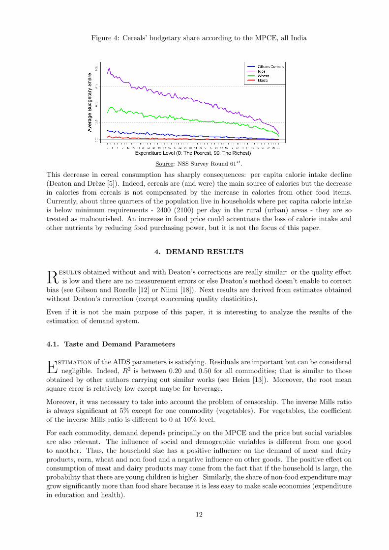
Figure 4: Cereals’ budgetary share according to the MPCE, all India

texteSource: NSS Survey Round 61st.

This decrease in cereal consumption has sharply consequences: per capita calorie intake decline(Deaton and Dreze [5]). Indeed, cereals are (and were) the main source of calories but the decreasein calories from cereals is not compensated by the increase in calories from other food items.Currently, about three quarters of the population live in households where per capita calorie intakeis below minimum requirements - 2400 (2100) per day in the rural (urban) areas - they are sotreated as malnourished. An increase in food price could accentuate the loss of calorie intake andother nutrients by reducing food purchasing power, but it is not the focus of this paper.

4. DEMAND RESULTS

Results obtained without and with Deaton’s corrections are really similar: or the quality effectis low and there are no measurement errors or else Deaton’s method doesn’t enable to correct

bias (see Gibson and Rozelle [12] or Niimi [18]). Next results are derived from estimates obtainedwithout Deaton’s correction (except concerning quality elasticities).

Even if it is not the main purpose of this paper, it is interesting to analyze the results of theestimation of demand system.

4.1. Taste and Demand Parameters

Estimation of the AIDS parameters is satisfying. Residuals are important but can be considerednegligible. Indeed, R2 is between 0.20 and 0.50 for all commodities; that is similar to those

obtained by other authors carrying out similar works (see Heien [13]). Moreover, the root meansquare error is relatively low except maybe for beverage.

Moreover, it was necessary to take into account the problem of censorship. The inverse Mills ratiois always significant at 5% except for one commodity (vegetables). For vegetables, the coefficientof the inverse Mills ratio is different to 0 at 10% level.

For each commodity, demand depends principally on the MPCE and the price but social variablesare also relevant. The influence of social and demographic variables is different from one goodto another. Thus, the household size has a positive influence on the demand of meat and dairyproducts, corn, wheat and non food and a negative influence on other goods. The positive effect onconsumption of meat and dairy products may come from the fact that if the household is large, theprobability that there are young children is higher. Similarly, the share of non-food expenditure maygrow significantly more than food share because it is less easy to make scale economies (expenditurein education and health).

12

4.2. Elasticities

Elasticities are easily obtained from the AIDS (the formulas given by Ramadam and Ulimwengu[20] are adapted because the inverse Mills ratio depends also on prices and on the total ex-

penditure). Price elasticities are really small; a majority is between -0.05 and 0.05. Elasticities arereported on Table 7 and Table 8 of the Appendix. Moreover, demand is not yet stable; the changesin elasticities between 1993 and 2004 underline that10.

Indeed, consumption pattern is changing quickly (see past Section) that explains why the elasticitieshave changed since 1993. Elasticities reflect demand so if demand changes, the values of elasticitiesmust change. For instance, the own-price elasticity of vegetables was equal to -1.12 in 1993 anddecreased to -0.59 in 2005 in the urban sector. In parallel, the own-price elasticity of coarse cereals(other cereals and maize) decreased between 1993 and 2004. There is also an income effect: theexpenditure elasticity of cereal became negative and this of vegetables and fruits are positive andrelatively high. That can explain the substitution observed between cereals and vegetables. Thisfinding underscores the changes occurred on consumption pattern.

Table 3: Expenditure Elasticity

Vegetables Spices Starchy BeverageRural 0.72

(0.02)0.67(0.01)

0.05(0.03)

1.73(0.09)

Urban 0.57(0.02)

0.48(0.02)

0.22(0.04)

1.24(0.10)

Corn Wheat Rice OilRural 0.59

(0.05)−0.55(0.04)

−0.42(0.06)

0.62(0.01)

Urban 0.93(0.01)

−0.63(0.06)

−0.14(00.06)

0.48(0.02)

Pulse Meat Other CerealRural 0.66

(0.01)1.88(0.03)

0.18(0.04)

Urban 0.54(0.02)

1.07(0.01)

−0.13(0.08)

Sugar Fruits Non FoodRural 0.83

(0.02)1.66(0.05)

1.23(0.01)

Urban 0.46(0.02)

1.33(0.03)

1.25(0.01)

texteSource: Author’s calculations based on the NSS Data Round 61st. The figures in brackets are obtained from 1,000replications of the bootstrap using the cluster-level data and are defined as half the length of the interval around thebootstrapped mean that contains 0.638 (the fraction of a normal random variable within two standard deviations ofthe mean) of the bootstrap replication.

Expenditure elasticities (Table 3) confirm that cereals became an inferior good, at least for riceand wheat. The expenditure elasticities of corn and other cereals (in the rural areas) are positive,but the estimation is not good because a lot of households don’t consume these commodities. Theexpenditure elasticities were always positive in 1993 for all the cereals. It was in last decade thatcereals became an inferior good. It cannot explain why cereal consumption declined between 1983and 1993, but it could, in part, explain why, since 1993, cereal consumption has declined.

Naturally, non food items, beverage, meat and fruits are luxury goods. For meat and non fooditems, consumption patterns consolidate this finding; indeed, the main part of the increase in realper capita expenditure is followed by an increase in non food expenditure. Kumar [16] noticedalso an important increase in meat expenditure between 1983 and 2000 (+65-70% of the budgetaryshare). The other commodities are normal goods.

10Expenditure elasticities derived frome the 50th Round of the NSS Survey are given in Appendix, Table 9

13

While meat is a product whose demand is very elastic to a variation in expenditure (and thereforeincome) in the rural areas (1.88), it is much less in the urban areas (1.07). Except for starchy,corn, rice and non-food goods, demand for necessary or luxury goods is less elastic in the urbansector than in the rural areas and more elastic concerning inferior goods. Urban households mayprefer maintaining a diversified consumption that’s why demand is less elastic in case of a changeprice.

Except the own-price elasticity of corn demand in the rural areas all own-price elasticities are neg-ative (Table 4). Demands in spices, wheat and other cereals are elastic (elasticity greater than onein absolute value) in both rural and urban areas; demand for other goods is not elastic. The lesselastic demands in the urban areas are sugar (-0.20) and non-food goods (-0.34); in the rural areasstarchy (-0.32) and sugar (-0.31) are the less elastic.

Table 4: Own-Price Elasticity

Vegetables Spices Starchy BeverageRural −0.65

(0.03)−1.01(0.01)

−0.32(0.03)

−0.56(0.02)

Urban −0.59(0.06)

−1.00(0.03)

0.15(0.20)

−0.49(0.03)

Corn Wheat Rice OilRural 3.14

(3.93)−0.90(0.04)

−0.42(0.04)

−0.85(0.04)

Urban −57.22(45.83)

−1.10(0.06)

−0.76(0.09)

−0.84(0.09)

Pulse Meat Other CerealRural −0.43

(0.03)−0.45(0.01)

−2.68(0.27)

Urban −0.48(0.07)

−0.79(0.03)

−4.28(2.08)

Sugar Fruits Non FoodRural −0.31

(0.05)−0.76(0.01)

−0.52(0.02)

Urban −0.20(0.09)

−0.84(0.02)

−0.36(0.02)

texte

Source: Author’s calculations from NSS Data Round 61st.

Cereal demand is more elastic in the urban area. Urban consumption depends less on cereal; urbanhouseholds have already diversified their consumption and are less dependent to cereal to feed them.So they can substitute more easily cereals to other food if the price of cereal increases. Householdsseem to prefer rice rather wheat. Indeed, wheat demand is more elastic than rice demand andMoreover, the expenditure elasticity is higher for rice (rice demand decreases more slowly if totalexpenditure increases than wheat demand). Main substitutes of cereals are other cereals (Table5). This finding is quite normal. Substitution is priority done among similar commodities. Thatcan explain in part why price elasticities are so small, especially own-price elasticities. Indeed, thesubstitution may take place first among the group. For instance, the main substitute of cucumbermay be another vegetables and so substitution among groups is less important than within agroup.

14

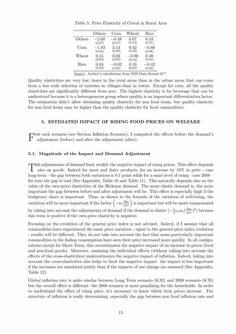
Table 5: Price Elasticity of Cereal in Rural Area

Others Corn Wheat RiceOthers −2.68

(0.27)−0.48(0.17)

0.67(0.14)

0.43(0.21)

Corn −1.83(0.64)

3.14(3.93)

0.42(0.52)

−0.80(0.98)

Wheat 0.15(0.03)

0.03(0.03)

−0.90(0.04)

0.40(0.04)

Rice 0.04(0.02)

−0.02(0.03)

0.18(0.02)

−0.42(0.04)

texte

Source: Author’s calculations from NSS Data Round 61st.

Quality elasticities are very low; lower in the rural areas than in the urban areas that can comefrom a less wide selection of varieties in villages than in towns. Except for corn, all the qualityelasticities are significantly different from zero. The highest elasticity is for beverage that can beunderstood because it is a heterogeneous group where quality is an important differentiation factor.The estimation didn’t allow obtaining quality elasticity for non food items, but quality elasticityfor non food items may be higher than the quality elasticity for food commodities.

5. ESTIMATED IMPACT OF RISING FOOD PRICES ON WELFARE

For each scenario (see Section Inflation Scenario), I computed the effects before the demand’sadjustment (before) and after the adjustment (after).

5.1. Magnitude of the Impact and Demand Adjustment

The adjustments of demand limit weakly the negative impact of rising prices. This effect dependsalso on goods. Indeed for meat and dairy products, for an increase by 10% in price - case

long-term - the gap between both variations is 0.1 point while for a same level of rising - case 2008 –for corn the gap is void (See Appendix, Table 10 and Table 11). This naturally depends also on thevalue of the own-price elasticities of the Hicksian demand. The more elastic demand is, the moreimportant the gap between before and after adjustment will be. This effect is especially high if thebudgetary share is important. Thus, as shown in the formula of the variation of well-being, thevariation will be more important if the factor

(−wi

∆pi

p0i

)is important but will be more compensated

by taking into account the adjustments of demand if the demand is elastic (−12εiiwi(∆pi

p0i )2) becausethis term is positive if the own-price elasticity is negative.

Focusing on the evolution of the general price index is not advised. Indeed, if I assume that allcommodities have experienced the same price variation - equal to the general price index evolution- results will be different. They do not take into account the fact that some particularly importantcommodities in the Indian consumption have seen their price increased more quickly. In all configu-rations except for Short-Term, this overestimates the negative impact of an increase in prices (foodand non-food goods). Moreover, summing the individual effects (without taking into account theeffects of the cross-elasticities) underestimates the negative impact of inflation. Indeed, taking intoaccount the cross-elasticities also helps to limit the negative impact: the impact is less importantif the increases are simulated jointly than if the impacts of one change are summed (See Appendix,Table 12).

Global inflation rate is quite similar between Long Term scenario (6.32) and 2008 scenario (6.76)but the overall effect is different: the 2008 scenario is more penalizing for the households. In orderto understand the effect of rising price, it’s necessary to know which item prices increase. Thestructure of inflation is really determining, especially the gap between non food inflation rate and

15

food inflation rate, and after among the food commodities. The structure of inflation implies alsohigher or lower differences between rural and urban sector. Rural households are more vulnerableif food inflation is important. The differences may be lower if the increase in beverage price isimportant because the urban household will be more penalized than the rural households.

Table 6: Average of Welfare Variation after Including Demand Reactions

Long Short Year DecemberTerm Term 2008 2010

Rural −8.13(0.72)

−6.74(1.20)

−10.57(1.50)

−2.60(0.83)

Urban −7.43(0.75)

−7.49(1.03)

−9.31(1.52)

−2.08(0.85)

texte

Source: Author’s calculations from NSS Data Round 61st. The figures in brackets are standards errors.

In the rural areas, the increases in price of rice, wheat, meat, vegetables and non-food goodspenalize more the households. An increase by 10% in the price of these four goods decreases thewelfare by more than 1%, on average. On the contrary, a very important increase in the price ofstarchy, corn or other cereals has a void impact on the welfare. Thus, an increase by 12.5% in theprice of starchy decreases the well-being by 0.17% while an increase by 8% in the price of wheatdecreases the household’s welfare by 0.44% and an increase by 5% in non-food price decreases thewelfare by 2%.

The impacts are somewhat different in the urban environment. Indeed, the differences in theconsumption pattern and the values of price-elasticities lead to different effects. Thus, urbanhouseholds are more vulnerable to an increase in the price of rice, beverage, fruit and non-foodgoods than in the rural areas. However, the impact is lower in the urban areas than in the rural areasexcept for the Short-Term case (which is characterized by a very high increase in non-food prices).Thus, rural populations are the most vulnerable by inflation, particularly food inflation.

Next section tries to determine which households are the most vulnerable to rising food prices. Itfocuses on which variables have a significant (positive or negative) impact on the magnitude ofwelfare variation. Moreover, it attempts to determine at-risk populations for each scenario andexplain why.

5.2. Who Are the Most Vulnerable?

5.2.1. Poor vs. Rich

The MPCE explains the main part of the magnitude of the impact on welfare (See Tables 13 and 14of the Appendix). The effect is generally positive: the higher the MPCE is, the lower the negativeimpact on welfare is. Four goods, in fact luxury goods, can be distinguished: meat, beverage, fruitand non food items. For instance if the MPCE increases by 10%, the negative impact due to risingnon food price is increased by 0.01282 and the negative impact due to rising rice price is reducedby 0.00243. Non food budgetary share is also important to characterize the impact of rising price.Indeed, for a same increase in price (10%) the effect of non food share on the magnitude of theimpact of inflation varies from one to ten. For instance if non food share is reduced by one point,the negative impact of rising rice price is increased by 2.116 until the negative impact of rising fruitprice is increased by 0.161.

Both findings confirm that the poor households have not benefited from the growth on last yearsto improve their well-being because of the high inflation. They are penalized because they havelow MPCE and because they consume more food that negatively increases the magnitude of the

16

impact. Moreover, at a same non food share, they consume more cereals that also adversely affectthem.

The inflation of last five years penalized the poor household whereas in last year (2010) the richhouseholds were more negatively affected. The reversal on last year didn’t offset the impact of pastinflation characterized by high food price inflation. However, if, in the next years, the non foodinflation is higher than food inflation, the poor households will be less negatively affected by theinflation and will be able to improve their conditions. On the other hand, if food price inflation ishigher, their vulnerability will increase whereas the rich households will not be so much affectedby the inflation that will increase the disparities.

Moreover, having a regular income allows limiting the negative impact of an increase in price onwelfare for the main commodities, particularly cereals. This reinforces the vulnerability of poorhouseholds11 which are 86% declaring no regular income vs. 52% for the other households. Thusit is important to provide regular income to fight against vulnerability because households are lessvulnerable; they can plan their consumption, they no longer live from hand to mouth and are soless dependent to market price evolution.

Food inflation disadvantaged more strongly poor households whereas a higher increase in priceof luxury goods (whose expenditure elasticity is greater than 1) penalizes more rich households(decreasing relation with the logarithm of the MPCE).

5.2.2. Rural vs. Urban

Except for beverage and non food, rural households are, on average, as much or more adverselyaffected by rising food price, all things being equal (for instance at a same level of MPCE). Anexplanation can be found on the values of price elasticities. Indeed, rural demand is less elasticthan urban demand and so the households don’t adjust enough their consumption to limit thenegative impact on welfare. Moreover, even if the self-employed in rural non agriculture (they areon average richer than the other rural households) are more negatively affected by rising cerealprices than casual laborers on the urban areas (they are on average poorer than the other urbanhouseholds). For the other items, casual laborers are more adversely affected.

Thus, rising cereal price affected more negatively all the rural households, whereas for the othercommodities the at-risk populations are defined priority by expenditure level. However,this studydoesn’t take into account the effect on farmer income. Indeed, a majority of rural households workon the agricultural sector and so can benefit from an increase in food prices. The effect on incomewill be important if the increase in food price results of an increase in product price. On the otherhand, if the increase results of an increase in retail price, the winners may be the middlemen andnot the farmer.

In any case, if rural inflation is enough lower than urban inflation, rural households will be lessaffected by inflation and so the welfare level may converge to urban area; on the other hand if ruralinflation is higher the gap is accentuated and disparities may increase. But since 2006, inflationrate (YoY) is higher for agricultural laborers (CPI-AL) than for industrial worker (CPI-IW), sodisparities may increase between both sectors: rural households have been more negatively affected.That can reinforce existing disparities such as on poverty HCR gap (41.8% against 28.3% with thenew poverty lines defined recently, see Himanshu [15]).

Thus, the increase in price of four commodities affects particularly rural households with a low levelof expenditure - rice, spices, sugar and starchy - while three goods affect urban poor households:wheat, beverage and other food, other cereals and substitutes. The impact of an increase in rice

11For next figures, poor households are defined as the households whose the MPCE is less than 150% of the povertyline.

17

is naturally more important in the rural sector. Indeed, in the rural sector at the national level,rice represents 55% of cereal consumption against 49% in the urban areas; wheat represents 47%of the urban household’s cereal consumption against 30% for rural households, that’s why urbanhouseholds suffer most from an increase in wheat price.

5.2.3. SC/ST and Religion

Religious status is relevant to explain the magnitude of the impact of rising food even if the effecton the magnitude of welfare variation is lower than that of the expenditure level. Indeed, for mostof the items, the religious belonging can accentuate the vulnerability. This study focuses on threegroups: Hindus, Muslims and others (including Sikhs, Jain, Christian, Buddhist and other religiousminorities).

The main finding is an increase in the negative impact of rising meat price if the household is Mus-lim. Muslims are also more negatively affected by an increase in rice or starchy prices. Moreover,the own-price elasticity of meat demand is higher for Muslims (-0.84) than for the other religiousgroups (-0.86 for both groups).The share of Muslim who consumes meat is higher than the shareof Hindu. Both facts explain why Muslims are more negatively affected by an increase in meatprice. The households which are not Hindu are also more negatively affected by an increase inmeat prices.

For the six main budgetary shares (rice, wheat, vegetables, meat, beverage and non food items),the Scheduled Caste and the Scheduled Tribes are more negatively affected by an increase in pricethan the non SC/ST except for meat. The disparity among both groups is huge for rice, meat andnon food items. The positive effect of being SC/ST regarding the impact of a rising meat price onwelfare can be due to the less part of SC/ST consuming meat and among the meat consumers, theless important budgetary share. For the other 8 goods the effect of being SC/ST is positive butweak. Furthermore, the SC/ST are more negatively affected by an increase in price of the maincommodities.

5.2.4. Household composition

Woman vulnerability is confirmed. Indeed, if the householder is a woman, the impact on thehousehold’s welfare is as much or more negative than if the householder is a man (except for nonfood items). On average, the households whose householder is a woman devote a higher budgetaryshare to food good (59% vs. 57%). Thus, mechanically, food inflation affects them more negatively.On the other hand, marital status is not a relevant factor of vulnerability. Being never married,widowed or divorced are not systematically more penalizing than being married. Their consumptionpattern and elasticities are not enough sufficiently different to bring significantly different impactson the magnitude of welfare variation.

The household size is, in many cases, a factor of vulnerability for the households. Indeed, for mostof the commodities, the negative effect increases with the household size to reach its maximum whenthe household is composed of around ten people; after this threshold, the effect is still negative butless important (it concerns few households, around 3% of the population). However, for beverage,pulse and starchy the household size increases always the loss of well-being.

There are economy scales in consumption. So, at a same level of MPCE, a large household maylive in best comfort than a small household. The large household may save more per capita (savingrate increases with living standards). In case of an increase in prices, the large household may beso less negatively affected than the small household. However, the empirical results underscore anopposite effect. The divergence with the theoretical analysis can come from the weak developmentof saving access in India.

18

The proportion of children under 15 years in the household is always a variable which has asignificant effect on the impact of inflation on the household’s welfare. Having relatively manychildren in the household conducts to a decrease in the households’ well-being for meat and dairyproducts (which can be understood especially if the children are very young and should drink milk),wheat, beverage and other food, non-food goods, fruit and starchy. We can think that it is moredifficult to make economy scale on non food items (health, education are included) than in foodcommodities. The opposite effect on an increase in rice price and on an increase in wheat price issomething strange.

5.2.5. Governmental Program

Households which self-report hunger are more negatively affected by an increase in price except forrice and non food items. Moreover, the households which don’t receive a governmental program12

are less vulnerable. These findings confirm the extreme vulnerability of the poorest householdsto the inflation. Indeed, the households reporting hunger are on average poorer than the otherhouseholds. Moreover, in order to benefit from one of these programs the household must bedeclare disadvantageous households.

Current governmental programs don’t allow protecting this at-risk population in case of inflation.However,it is more difficult to insert into the analysis meals taken outside the household. Thisstudy simulates the impact of rising price of specific goods (vegetables, rice. . . ) whereas thoseprograms offer prepared meals or food as wage. The negative impact of inflation on the householdscan be overestimated because, for instance, the effect of having free meals at midday instead ofmaking own meal is underestimated.

On the other hand, having a ration card13 can limit the negative impact of inflation on the house-hold’s welfare. Indeed, households with a ration card are less negatively affected by an increasein cereal prices. Households are protected by restricted prices (Antodaya and BLP cards allow itsowner to buy rice and wheat at very low prices which are fixed).

This last finding mitigates the critics on the PDS and its failures. Indeed The PDS program iscritiqued because it fails to target the poorest households. Indeed“identifying the poor in a countrylike India is a formi-dable task”14. Moreover, Himanshu15 said “Historically, limiting food securityto BPL families has severely impaired the effective access to food for poor families. In particular,(i) large numbers of poor families did not have BPL cards, (ii) even when they had cards, accessto PDS was not automatic and, (iii) even if they had access to Public Distribution System (PDS),they did not receive the full entitlement of food.” I don’t question these problems but this workunderlines the positive effect for the households which have a ration card and which purchase foodon PDS shop. These programs of food security allow the households to mitigate the negative impactof inflation on welfare. However, I don’t distinguish cards and the positive effect can come fromthe other cards but the existence of a positive effect is set for the programs.

12Four governmental programs are effective: Food for Work, Annapoorna, ICDS and Midday Meal.13There are three types of food ration card: BLP, the Antodaya and others. The BLP (Below Poverty Line) card is

issued to households by the Government. The condition is, of course, to live below poverty line (threshold dependingon the sector and the State). This card allows buying on PDS (Public Distribution System) shops where prices arenormally lower at market prices (but is not always the case, a large existing traffic) Antodaya card is reserved to the”very poor”, it concerns the poorest households among those living below the poverty line. The beneficiaries of thiscard can purchase 25 kg of cereals at 2 INR/kg for wheat and 3 for rice. Other cards also allow accessing to limitedprice commodities but they are not described.

14PDS Forever? By Ashok Kotwal, Milind Murugkar, Bharat Ramaswami, published on EPW Vol xlvi no 2115http://www.india-seminar.com/2011/617/617 himanshu.htm

19

5.2.6. State Disparities

There are also disparities between states. Indeed, national average clears variations between states.Differences on the magnitude of the impact depend on commodity whose price increases. Theimpact of an increase in non food prices is quite homogenous among state whereas there are hugedifferences between states for wheat and rice. Indeed, Rajasthan, Bihar, Uttar Pradesh and MadhyaPradesh are strongly affected by an increase in wheat price: in average welfare decrease by 1% foran increase by 10% in prices. At the opposite, nineteen states are weakly affected (the welfaredecrease is lower than 0.2%).

Figure 5: Welfare Variation by State for 2008

texteSource: Author’s calculations from NSS Data Round 61st.

An increase in rice prices affects strongly the states on the East coast, specifically Manipur, Assam,Tripura, West Bengal, Chhattisgarh and Jharkhand. The decrease in welfare is higher than 2%.States on North-West are more protected (the welfare decrease is lower than 0.5%).

For the ”2008” case, the variations are enough significant. The following map (Figure 5) showsthese disparities. Four groups (i.e. quartiles) are made. The limits of each quartile are given to becompared with the national average (-10.31%).

20

5.3. The Four Inflation Scenarios

Inlong term perspective (i.e. according to the Long Term scenario), the most vulnerable house-holds are the poorest rural households (low monthly expenditure per capita). These households

dedicated a small share of their budget to non-food goods. The households, less educated, is com-posed by few children and many women; the householder is old enough (about 50 years). Muslimsare protected but the non-Hindu and non-Muslim are more adversely affected by the inflationbecause the increase in meat price was relatively lower than the increase in other food prices.Agricultural laborers without lands and households without a regular source of income are alsoparticularly affected by inflation. Households self-reporting hunger are at risk populations.

A bout of inflation such as that of December 2010 (see Table 14 of the Appendix) affects negativelythe poorest households because of very high food price inflation. However,that must be checked byother studies. Indeed, this work is not based on data of December 2011; it’s just a simulation ofthe potential effect of the inflation on the household’s welfare. The result of the simulation basedon inflation of December 2011 is pessimistic by the magnitude of the impact (a third of the impactof Long Term scenario but just for one month and not one quarter) and by the most affectedhouseholds which are yet disadvantaged.

The food price crisis in 2008 had affected hardest rural households. However,affluent and educatedhouseholds whose householder is a 60 year-old woman are the most vulnerable. Apart from this,at-risk populations have the same characteristics as those of the ”Long term” case.

Thus in India the most disadvantaged households are not the most affected by global food pricesepisode in 2008 because cereals have experienced the highest increase in prices - the Governmenttook drastic measures to limit the increase in the price of cereals such as the stop of exports- but food goods such as meat and dairy products consumed by richer households. RememberHowever,that these positive effects of the increase in prices on producers are not taken into ac-count.

On the other hand, on short term perspective (Short Term scenario) the most affected populationsby ”Short term” inflation are so different. Indeed, the richest urban households, devoting a highshare of their spending on non-food goods are the most negatively affected by the rise in price.The fact of not having children under 15 years in the household and a high proportion of womenreinforces the effects as well as a low level of education. Households working on their own account,but with no regular source of income are among the most vulnerable households. Again having afood ration card increases the vulnerability of households.

6. CONCLUDING REMARKS

This paper examined the impact of food inflation on the household’s welfare. The main findingsare as follows.

First, consumption pattern has changed since 1993. Non food expenditure has increased whereashouseholds have diversified food consumption. Cereal, particularly coarse cereal, consumptionhas declined. Many authors characterized these changes and tried to explain it. It is not thefocus of the article but it is important to understand why elasticities between 1993 and 2004changed. Consumption pattern is not yet stable in an emergent country like India. These evolutionsimpact the demand reactions and so the values of price and expenditure elasticities; the effect onwelfare.

Secondly, expenditure elasticities allow classifying commodities on three groups: inferior goods

21

(cereals), normal goods and luxury goods (fruit, non food, beverage and meat). Elasticities on therural areas are not the same than in the urban areas. Indeed, urban demand is less elastic except forinferior goods. Moreover, price elasticities are small but in majority significantly different to zero.Demand is not elastic so inflation will impact severely the households because their consumptionpattern would not change a lot. However,some goods are substitutable, for instance cereals. Ifwheat price increases, rice demand will increase to substitute wheat in order to limit the negativeimpact.

Then, the household’s welfare has increased in India since 1993. Improvements in health’s access,electricity, less physical work, increase of real income per capita explain this improvement butsome factors have limited the improvement of well-being as inflation. Indeed, food inflation affectsnegatively the welfare of households. The average of decrease is around 8-10% for each scenario(except December 2010 but we can’t compare directly this scenario with the other three). Varia-tions are computed from the elasticities obtained with the NSS data (Round 61st) and assumingthat elasticities have been constant since 2005. The most penalizing increases in price concerncereals and non-food goods, on the contrary an increase in fruit price is not really penalizing forthe households. Indeed, the structure of inflation is important to compute the decrease in thehousehold’s welfare.

Next, different structures of inflation affect negatively different households. Indeed, if the price offood, especially cereals, increases rapidly, the most vulnerable households are the rural householdswith a low level of expenditure. If the highest increase in price concerns non-food items, the mostnegatively affected households are the rich household living in the urban areas. The household size,the age and the sex of the householder are characteristics which impact the value of the decrease inwell-being but differently according to the structure of inflation. Food inflation increases inequalities(by impacting more the poorest) whereas non-food inflation seems to reduce (by impacting therichest).

These results on the impact of inflation on the household’s welfare are far from conclusive. Samestudies with recent data, with price data, including the supply side and the effects on others markets(labor market for instance) must be carried on such as a study which doesn’t focus on price toexplain welfare’s variation.

22

References

[1] Chern, Wen S. and alii (2003): Analysis of The Food Consumption of Japanese Households,FAO, Economic and Social Development, Paper 152

[2] Deaton, Angus (1987): Estimation of Own- and Cross-Price Elasticities from Household SurveyData, Journal of Econometrics 36, pp 7-30

[3] Deaton, Angus (1997): The Analysis of Household Surveys: A Microeconometric Approach toDevelopment Policy, Johns Hopkins University Press

[4] Deaton, Angus (2008): Price Trends in India and Their Implications for Measuring Poverty,Economic & Political Weekly, 9 February, pp 43-49.

[5] Deaton, Angus and Jean Dreze (2009): “Food and Nutrition in India: Facts and Interpreta-tions”, Economic & Political Wee

[6] Deaton, Angus and Valerie Kozel (2005): The Great India Poverty Debate, Macmillankly, 14February, pp 42-65.

[7] Deaton, Angus and John Muellbauer (1980): An Almost Ideal Demand System, AmericanEconomic Review 70, pp 521-532

[8] Deaton, Angus and Salman Zaidi (2003): Guidelines for Constructing Consumption Aggre-gates For Welfare Analysis

[9] Deaton, Angus and Alessandro Tarozzi (2000): Prices and poverty in India, Research Programin Development Studies, Princeton University

[10] Dorin, Bruno (2002): Agriculture et Alimentation de l’Inde, (Paris : INRA).

[11] Filmer, Deon and Lant H. Pritchett (2001): Estimating Wealth Effects without ExpenditureData or Tears: An Application to Educational Enrolments in States of India. Demography38(1), pp 115-32.

[12] Gibson, John and Scott Rozelle (2002): Is a Picture Worth a Thousand Unit Values? PriceCollection Methods, Poverty Lines and Price Elasticities in Papua New Guinea, NortheastUniversities Development Consortium Conference

[13] Heien, Dale and Cathy R. Wessells (1990): Demand Systems Estimation with Microdata: ACensored Regression Approach, Journal of Business & Economic Statistics, 8(3), pp 365-371

[14] Himanshu (2007): Recent Trends in Poverty and Inequality: Some Preliminary Results, Eco-nomic & Political Weekly, 14 February, pp 42-65.

[15] Himanshu (2010): Towards New Poverty Lines for India, Economic & Political Weekly, volXLV No 1

[16] Kumar, Praduman, Mruthyunjaya, and Madan M. Dey (2007): Long-term changes in Indianfood basket and nutrition, Economic & Political Weekly 42(35), 1 September, pp 3567–72.

[17] Minot, Nicholas and Francesco Goletti (2000): Rice market liberalization and poverty in VietNam. Research Report 114, International Food Policy Research Institute (IFPRI).

[18] Niimi, Yoko (2005): An Analysis of Household Responses to Price Shocks in Vietnam: CanUnit Values Substitute for Market Prices?, PRUS Working Paper no. 30

[19] Rao, C H Hanumantha (2000): Declining Demand for Foodgrains in Rural India: Causes andImplications, Economic & Political Weekly 35(2), 22 January, pp 201–06.

23

[20] Ulimwengu, John R and Racha Ramadam (2009) How Does Food Price Increase Affect Ugan-dan Households? An Augmented Multimarket Approach. IFPRI Discussion Paper no 00884

[21] Zezza, Alberto and al. (2008): The impact of rising food prices on the poor. ESA WorkingPaper No 08-07. Food and Agriculture Organization (FAO).

[22] National Sample SurveyOrganization, National Seminar on NSS 61st Round Survey Report

[23] World Bank (2000), India: Policies to Reduce Poverty and Accelerate Sustainable Develop-ment, Report No 19471

[24] Ferreira Francisco H. G., and alii (May 2011), Rising Food Prices and Household Welfare:Evidence from Brazil in 2008, Policy Research Working Paper 5652

A. APPENDIX

Key lecture for the two following tables: The figures in brackets are obtained from 1,000 replica-tions of the bootstrap using the cluster-level data and are defined as half the length of the intervalaround the bootstrap mean that contains 0.638 (the fraction of a normal random variable withintwo standard deviations of the mean) of the bootstrap replication.

24

Urb

an

Veg

eSpic

esSta

rchy

Oil

Puls

eM

eat

Oth

ers

Corn

Whea

tR

ice

Bev

erages

Sugar

Fru

itN

on

food

table

sC

erea

lsand

Oth

er

Exp

endit

ure

0.7

20.6

70.0

50.6

20.6

61.8

80.1

80.5

9-0

.55

-0.4

21.7

30.8

31.6

61.2

3

Ela

stic

ity

(0.0

2)

(0.0

1)

(0.0

3)

(0.0

1)

(0.0

1)

(0.0

3)

(0.0

4)

(0.0

5)

(0.0

4)

(0.0

6)

(0.0

9)

(0.0

2)

(0.0

5)

(0.0

1)

PriceElasticity

Veg

etable

s-0

.32

0.1

3-0

.75

0.1

10.2

00.1

00.9

6-2

.06

0.0

4-0

.41

0.0

30.2

33.4

90.0

4

(0.0

2)

(0.0

1)

(0.0

3)

(0.0

1)

(0.0

1)

(0.0

0)

(0.0

6)

(0.1

1)

(0.0

2)

(0.0

1)

(0.0

3)

(0.0

2)

(0.1

4)

(0.0

7)

Spic

e0.2

4-0

.95

0.4

00.0

60.1

50.0

3-0

.30

-0.4

90.1

8-0

.32

0.0

50.0

50.3

90.1

3

(0.0

2)

(0.0

1)

(0.0

2)

(0.0

0)

(0.0

1)

(0.0

0)

(0.0

3)

(0.0

3)

(0.0

2)

(0.0

2)

(0.0

0)

(0.0

2)

(0.0

5)

(0.0

8)

Sta

rchy

-0.2

10.0

1-1

.51

0.0

90.0

20.0

71.0

8-0

.08

-0.4

0-0

.11

0.0

9-0

.21

0.0

5-0

.03

(0.0

1)

(0.0

1)

(0.1

2)

(0.0

1)

(0.0

2)

(0.0

0)

(0.0

8)

(0.0

4)

(0.0

3)

(0.0

1)

(0.0

1)

(0.0

2)

(0.2

0)

(0.0

8)

Mea

t0.1

80.1

10.7

3-0

.21

0.0

20.0

6-0

.25

4.2

6-0

.26

-0.0

20.0

1-0

.01

-6.4

80.3

2

(0.0

1)

(0.0

1)

(0.0

4)

(0.0

4)

(0.0

2)

(0.0

1)

(0.0

5)

(0.2

1)

(0.0

2)

(0.0

3)

(0.0

3)

(0.0

3)

(0.2

6)

(0.3

9)

Puls

e0.1

50.1

9-0

.01

0.1

1-0

.76

0.0

2-0

.33

-3.2

0-0

.15

-0.2

40.0

1-0

.06

4.2

00.0

7

(0.0

2)

(0.0

1)

(0.0

6)

(0.0

1)

(0.0

3)

(0.0

1)

(0.0

2)

(0.1

5)

(0.0

2)

(0.0

1)

(0.0

2)

(0.0

3)

(0.2

2)

(0.0

1)

Oil

0.2

30.0

90.6

10.1

00.0

4-0

.86

-0.2

80.5

7-0

.12

1.0

1-0

.30

-0.0

6-0

.55

0.1

1

(0.0

0)

(0.0

0)

(0.0

2)

(0.0

0)

(0.0

1)

(0.0

1)

(0.0

3)

(0.0

2)

(0.0

2)

(0.0

3)

(0.0

1)

(0.0

1)

(0.0

3)

(0.0

5)

Oth

ers

0.1

10.0

10.4

90.2

0-0

.18

-0.0

5-1

.14

0.0

3-0

.19

0.4

9-0

.15

-0.1

8-0

.20

0.1

9

Cer

eals

(0.0

8)

(0.0

0)

(0.0

6)

(0.0

1)

(0.0

1)

(0.0

1)

(0.0

2)

(0.0

2)

(0.0

3)

(0.0

3)

(0.0

1)

(0.0

1)

(0.0

8)

(0.2

1)

Corn

0.0

5-0

.05

0.0

1-0

.18

-0.0

90.0

2-0

.44

-1.3

3-0

.43

0.2

2-0

.03

0.1

10.5

7-0

.15

(0.0

1)

(0.0

1)

(0.0

6)

(0.0

2)

(0.0

1)

(0.0

0)

(0.0

3)

(0.2

3)

(0.0

2)

(0.0

1)

(0.0

2)

(0.0

2)

(0.1

4)

(0.2

0)

Whea

t0.0

70.2

2-1

.29

-0.0

7-0

.11

-0.0

3-0

.40

-5.0

6-3

.00

2.0

70.1

9-0

.62

6.4

90.1

6

(0.0

2)

(0.0

1)

(0.0

6)

(0.0

1)

(0.0

1)

(0.0

1)

(0.0

3)

(0.1

8)

(0.1

1)

(0.0

4)

(0.0

1)

(0.0

3)

(0.2

8)

(0.0

7)

Ric

e-0

.46

-0.1

7-0

.23

0.1

5-0

.20

0.6

51.2

94.1

83.2

9-2

.71

0.4

80.6

2-5

.06

-0.0

8

(0.0

2)

(0.0

1)

(0.0

5)

(0.0

1)

(0.0

1)

(0.0

2)

(0.0

4)

(0.1

8)

(0.0

9)

(0.0

6)

(0.0

2)

(0.0

2)

(0.2

1)

(0.1

3)

Bev

erages

0.0

50.0

00.2

9-0

.01

0.0

1-0

.12

-0.3

7-0

.12

0.1

80.2

8-0

.25

-0.2

30.1

50.0

0

and

Oth

er(0

.01)

(0.0

0)

(0.0

1)

(0.0

1)

(0.0

0)

(0.0

1)

(0.0

3)

(0.0

1)

(0.0

2)

(0.0

1)

(0.0

3)

(0.0

1)

(0.1

0)

(0.0

2)

Sugar

0.1

30.0

3-0

.45

-0.0

5-0

.10

-0.0

10.0

4-2

.57

-0.3

80.2

4-0

.13

-0.1

94.2

0-0

.04

(0.0

1)

(0.0

1)

(0.0

5)

(0.0

1)

(0.0

2)

(0.0

0)

(0.0

3)

(0.1

3)

(0.0

1)

(0.0

1)

(0.0

1)

(0.0

4)

(0.1

8)

(0.0

7)

Fru

it-0

.03

0.0

4-0

.10

0.0

50.0

3-0

.03

0.4

2-0

.07

-0.0

2-0

.29

0.0

60.1

2-0

.67

0.0

7

(0.0

0)

(0.0

1)

(0.0

1)

(0.0

1)

(0.0

0)

(0.0

1)

(0.0

3)

(0.0

1)

(0.0

3)

(0.0

3)

(0.0

2)

(0.0

0)

(0.0

1)

(0.0

4)

Non

food

-0.4

00.8

01.8

5-0

.11

0.7

80.1

3-1

.95

7.7

30.9

0-0

.41

0.0

50.2

5-8

.67

0.3

2

(0.0

3)

(0.0

4)

(0.1

1)

(0.0

3)

(0.0

1)

(0.4

6)

(0.1

8)

(0.3

5)

(0.0

8)

(0.0

6)

(0.1

2)

(0.0

5)

(0.8

3)

(0.8

3)

Ela

stic

itie

sare

pre

sente

dso

that

the

colu

mns

are

the

goods

whose

pri

ces

are

changin

gand

the

row

sth

egoods

whose

quanti

ties

are

bei

ng

aff

ecte

d

Sourc

e:A

uth

or’

sca

lcula

tions

from

NSS

Data

Round

61st

.

Tab

le7:

Pri

ceE

last

icit

yof

Com

pens

ated

Dem

and

inR

ural

Are

a,E

stim

ated

byth

eA

IDS

wit

hD

emog

raph

icT

rans

lati

onan

dSe

lect

ion

Bia

sC

orre

ctio

nl

25

Urb

an

Veg

eSpic

esSta

rchy

Oil

Puls

eM

eat

Oth

ers

Corn

Whea

tR

ice

Bev

erages

Sugar

Fru

itN

on

food

table

sC

erea

lsand

Oth

er

Exp

endit

ure

0.5

70.4

80.2

20.4

80.5

41.0

7-0

.13

0.9

3-0

.63

-0.1

41.2

40.4

61.3

31.2

5

Ela

ast

icit

y(0

.02)

(0.0

2)

(0.0

4)

(0.0

2)

(0.0

2)

(0.0

1)

(0.0

8)

(0.0

1)

(0.0

6)

(0.0

6)

(0.1

0)

(0.0

2)

(0.0

3)

(0.0

1)

PriceElasticity

Veg

etable

s-0

.26

0.1

4-0

.17

0.3

20.0

10.0

5-0

.01

-0.0

4-0

.15

-0.4

30.0

00.0

70.0

30.3

0

(0.0

2)

(0.0

1)

(0.0

1)

(0.0

2)

(0.0

2)

(0.0

2)

(0.0

1)

(0.0

0)

(0.0

2)

(0.0

2)

(0.0

1)

(0.0

1)

(0.0

1)

(0.0

5)

Spic

e0.0

8-0

.99

0.0

60.1

00.1

10.0

2-0

.04

-0.0

30.1

1-0

.42

-0.0

4-0

.09

0.0

61.5

0

(0.0

1)

(0.0

2)

(0.0

1)

(0.0

2)

(0.0

2)

(0.0

1)

(0.0

1)

(0.0

0)

(0.0

2)

(0.0

3)

(0.0

1)

(0.0

1)

(0.0

1)

(0.0

6)

Sta

rchy

-1.0

10.7

5-0

.90

0.8

70.1

90.5

30.6

4-0

.12

-2.0

9-0

.16

0.0

8-0

.33

-0.1

02.3

9

(0.0

7)

(0.0

6)

(0.0

8)

(0.1

0)

(0.1

1)

(0.0

5)

(0.0

3)

(0.0

5)

(0.0

7)

(0.0

6)

(0.0

2)

(0.0

8)

(0.0

2)

(0.1

7)

Mea

t0.2

40.0

50.0

7-0

.35

-0.1

4-0

.03

0.0

50.0

6-0

.27

0.0

4-0

.08

-0.0

60.0

70.5

5

(0.0

2)

(0.0

1)

(0.0

1)

(0.0

4)

(0.0

3)

(0.0

1)

(0.0

1)

(0.0

1)

(0.0

2)

(0.0

2)

(0.0

1)

(0.0

2)

(0.0

1)

(0.0

6)

Puls

e0.0

10.0

60.0

5-0

.31

-0.2

8-0

.06

0.0

9-0

.10

-0.1

2-0

.33

-0.0

2-0

.07

0.0

60.9

6

(0.0

2)

(0.0

2)

(0.0

2)

(0.0

4)

(0.0

6)

(0.0

1)

(0.0

1)

(0.0

1)

(0.0

2)

(0.0

3)

(0.0

1)

(0.0

3)

(0.0

1)

(0.0

7)

Oil

0.0

20.0

00.0

3-0

.03

0.0

1-0

.69

-0.0

60.0

10.0

90.1

1-0

.12

0.0

00.0

20.6

0

(0.0

1)

(0.0

0)

(0.0

0)

(0.0

1)

(0.0

1)

(0.0

1)

(0.0

1)

(0.0

0)

(0.0

1)

(0.0

2)

(0.0

1)

(0.0

0)

(0.0

1)

(0.0

2)

Oth

ers

1.6

9-0

.97

2.5

4-1

.62

0.4

5-1

.33

-2.1

4-0

.81

0.7

5-0

.25

-0.8

00.6

30.7

7-3

.06

Cer

eals

(0.1

2)

(0.0

6)

(0.1

3)

(0.1

4)

(0.0

6)

(0.0

9)

(0.0

6)

(0.0

5)

(0.1

1)

(0.1

1)

(0.0

5)

(0.0

6)

(0.0

5)

(0.3

4)

Corn

-8.0

4-1

.53

-0.3

617.4

1-1

1.2

11.3

70.6

3-2

.60

-15.3

312.5

7-0

.45

-10.3

3-0

.03

24.1

5

(0.9

9)

(0.1

9)

(0.0

8)

(2.0

8)

(1.3

4)

(0.1

5)

(0.0

8)

(0.1

9)

(1.8

6)

(1.5

3)

(0.0

6)

(1.2

6)

(0.0

1)

(2.8

7)

Whea

t-0

.24

0.0

2-0

.37

-0.5

3-0

.17

0.2

60.2

6-0

.09

-3.4

52.7

6-0

.16

-0.3

20.0

81.7

2

(0.0

2)

(0.0

2)

(0.0

1)

(0.0

3)

(0.0

2)

(0.0

2)

(0.0

3)

(0.0

1)

(0.0

7)

(0.0

7)

(0.0

3)

(0.0

1)

(0.0

2)

(0.1

3)

Ric

e-0

.35

-0.5

0-0

.08

-0.2

2-0

.30

0.1

8-0

.13

0.0

81.8

8-1

.94

0.1

40.0

8-0

.16

1.1

0

(0.0

2)

(0.0

2)

(0.0

1)

(0.0

3)

(0.0

2)

(0.0

4)

(0.0

2)

(0.0

1)

(0.0

6)

(0.0

8)

(0.0

2)

(0.0

1)

(0.0

2)

(0.1

2)

Bev

erages

0.0

10.0

00.0

1-0

.09

0.0

0-0

.26

-0.0

60.0

1-0

.08

0.1

50.3

7-0

.06

-0.0

10.1

1

and

Oth

er(0

.02)

(0.0

1)

(0.0

1)

(0.0

2)

(0.0

2)

(0.0

2)

(0.0

1)

(0.0

2)

(0.0

1)

(0.0

2)

(0.1

0)

(0.0

1)

(0.0

6)

(0.1

1)

Sugar

0.1

5-0

.11

-0.1

50.0

40.0

0-0

.07

0.0

3-0

.19

-0.6

80.2

7-0

.25

0.0

00.1

00.7

5

(0.0

2)

(0.0

3)

(0.0

2)

(0.0

4)

(0.0

5)

(0.0

2)

(0.0

2)

(0.0

2)

(0.0

2)

(0.0

3)

(0.0

1)

(0.0

5)

(0.0

1)

(0.0

7)

Fru

it2.2

50.2

4-0

.17

-4.0

82.6

6-0

.15

-0.1

80.4

34.3

2-3

.12

0.1

12.5

6-0

.68

-5.8

4

(0.1

6)

(0.0

3)

(0.0

2)

(0.3

5)

(0.2

3)

(0.0

4)

(0.0

2)

(0.0

4)

(0.3

2)

(0.2

6)

(0.0

2)

(0.2

1)

(0.0

1)

(0.5

1)

Non

food

0.0

30.0

80.0

20.0

70.0

50.1

30.0

4-0

.01

0.1

10.0

90.0

40.0

20.0

2-0

.57

(0.0

1)

(0.0

1)

(0.0

2)

(0.0

7)

(0.0

1)

(0.0

1)

(0.0

4)

(0.0

4)

(0.0

1)

(0.0

3)

(0.0

1)

(0.0

1)

(0.0

1)

(0.1

5)

Ela

stic

itie

sare

pre

sente

dso

that

the

colu

mns

are

the

goods

whose

pri

ces

are

changin

gand

the

row

sth

egoods

whose

quanti

ties

are

bei

ng

aff

ecte

d

Sourc

e:A

uth

or’

sca

lcula

tions

from

NSS

Data

Round

61st

.

Tab

le8:

Pri

ceE

last

icit

yof

Com

pens

ated

Dem

and

inU

rban

Are

a,E

stim

ated

byth

eA

IDS

wit

hD

emog

raph

icT

rans

lati

onan

dSe

lect

ion

Bia

sC

orre

ctio

n

26

Whea

tR

ice

Oth

erC

erea

lsSta

rchy

Oil

Spic

eP

uls

eV

eget

able

sM

aiz

eSugar

Mea

tF

ruit

sB

ever

age

Non

Food

Rura

l0.0

5-0

.02

0.2

40.4

70.6

30.6

90.6

60.7

60.8

60.8

82.0

11.5

23.5

21.0

5

Urb

an

0.0

1-0

.34

-1.2

40.2

30.7

10.6

50.6

80.8

20.3

80.8

61.7

91.4

52.3

91.0

0

Tab

le9:

Exp

endi

ture

Ela

stic

itie

sde

rive

dfr

omth

e50

thR

ound

ofth

eN

SSSu

rvey

27

Urban: After/Before Long Term Short Term 2008 December 2010Vegetables -0.69/-0.71 -0.54/-0.55 -0.72/-0.75 -0.90/-0.93

(0.41)/(0.42) (0.32)/(0.33) (0.43)/(0.44) (0.53)/(0.55)Rice -0.55/-0.60 -0.11/-0.12 -0.84/-0.96 -0.03/-0.03

(0.50)/(0.55) (0.10)/(0.11) (0.77)/(0.89) (0.02)/(0.02)Wheat -0.36/-0.42 -0.03/-0.03 -0.47/-0.58 -0.01/-0.01

(0.37)/(0.43) (0.03)/(0.03) (0.43)/(0.48) (0.01)/(0.01)Corn 0.00/0.00 0.00/0.00 0.00/0.00 0.00/0.00

(0.03)/(0.03) (0.04)/(0.05) (0.03)/(0.04) (0.00)/(0.00)Others Cereals -0.07/-0.08 -0.05/-0.05 -0.10/-0.12 -0.02/-0.02

(0.21)/(0.24) (0.14)/(0.15) (0.30)/(0.38) (0.05)/(0.06)Pulse -0.26/-0.27 0.12/0.12 -0.53/-0.55 -0.04/-0.04

(0.16)/(0.16) (0.07)/(0.07) (0.31)/(0.32) (0.03)/(0.03)Starchy -0.09/-0.10 0.13/0.13 -0.18/-0.20 -0.08/-0.08

(0.11)/(0.12) (0.16)/(0.15) (0.21)/(0.23) (0.09)/(0.10)Spices -0.59/-0.67 -0.64/-0.72 -0.54/-0.60 -0.51/-0.56

(0.32)/(0.36) (0.34)/(0.38) (0.29)/(0.32) (0.27)/(0.30)Meat and -1.02/-1.06 -1.22/-1.27 -1.56/-1.65 -0.11/-0.11

dairy products (0.58)/(0.60) (0.69)/(0.72) (0.89)/(0.94) (0.06)/(0.06)Beverages and -0.54/-0.53 -0.19/-0.19 -1.14/-1.12 0.05/0.05

other (0.83)/(0.82) (0.30)/(0.29) (1.77)/(1.73) (0.07)/(0.07)Sugar -0.14/-0.14 0.29/0.29 -0.76/-0.76 -0.05/-0.05

(0.09)/(0.09) (0.20)/(0.20) (0.52)/(0.52) (0.04)/(0.04)Oil -0.16/-0.17 -0.46/-0.47 0.01/0.01 -0.05/-0.05

(0.09)/(0.09) (0.22)/(0.25) (0.00)/(0.00) (0.03)/(0.03)Fruits -0.20/-0.21 -0.33/-0.35 -0.25/-0.25 0.03/0.03

(0.16)/(0.17) (0.27)/(0.29) (0.20)/(0.21) (0.03)/(0.03)Non Food -2.50/-2.54 -4.45/-4.57 -1.84/-1.86 -0.36/-0.36

(0.68)/(0.69) (1.21)/(1.24) (0.50)/(0.51) (0.09)/(0.09)

Table 10: Average of Welfare Variation (%) in Rural Area for the Increase in Each Price Indepen-dently, Estimated by the AIDS

Rural: After/Before Long Term Short Term 2008 December 2010Vegetables -0.83/-0.86 -0.65/-0.67 -0.87/-0.90 -1.07/-1.12

(0.46)/(0.47) (0.36)/(0.37) (0.48)/(0.50) (0.59)/(0.62)Rice -0.98/-1.11 -0.21/-0.22 -1.45/-1.79 -0.05/-0.05

(0.83)/(0.94) (0.18)/(0.18) (1.24)/(1.53) (0.04)/(0.04)Wheat -0.44/-0.51 -0.03/-0.03 -0.58/-0.70 -0.02/-0.02

(0.47)/(0.54) (0.03)/(0.04) (0.62)/(0.75) (0.01)/(0.01)Corn -0.03/-0.03 -0.05/-0.05 -0.04/-0.04 0.00/0.00

(0.17)/(0.18) (0.25)/(0.28) (0.20)/(0.22) (0.01)/(0.01)Other Cereal -0.17/-0.18 -0.11/-0.11 -0.25/-0.28 -0.04/-0.04

(0.43)/(0.47) (0.28)/(0.29) (0.64)/(072) (0.10)/(0.11)Pulse -0.33/-0.34 0.15/0.15 -0.66/-0.71 -0.05/-0.05

(0.18)/(0.19) (0.08)/(0.08) (0.36)/(0.39) (0.03)/(0.03)Starchy -0.18/-0.20 0.29/0.26 -0.34/-0.42 -0.16/-0.17

(0.18)/(0.20) (0.30)/(0.26) (0.34)/(0.42) (0.16)/(0.18)Spice -0.83/-0.92 -0.88/-0.99 -0.75/-0.83 -0.70/-0.77

(0.35)/(0.39) (0.38)/(0.43) (0.32)/(0.35) (0.30)/(0.32)Continued on next page. . .

28

. . . Continue

Rural: After/Before Long Term Short Term 2008 December 2010Meat and -1.07/-1.12 -1.27/-1.34 -1..62/-1.74 -0.11/-0.11

dairy products (0.78)/(0.81) (0.93)/(0.99) (1.18)/(1.27) (0.08)/(0.08)Beverages -0.32/-0.33 -0.12/-0.12 -0.68/-0.69 0.03/0.03

and Others (0.48)/(0.48) (0.18)/(0.18) (1.00)/(1.01) (0.04)/(0.04)Sugar -0.18/-0.19 0.42/0.39 -0.82/-1.03 -0.07/-0.07

(0.13)/(0.13) (0.27)/(0.26) (0.67)/(0.69) (0.05)/(0.05)Oil -0.21/-0.21 -0.60/-0.61 0.01/0.01 -0.06/-0.06

(0.10)/(0.10) (0.28)/(0.28) (0.00)/(0.00) (0.08)/(0.08)Fruits -0.15/-0.16 -0.25/-0.26 -0.19/-0.19 0.02/0.02

(0.17)/(0.18) (0.28)/(0.29) (0.21)/(0.22) (0.02)/(0.02)Non Food -1.99/-2.00 -3.56/-3.61 -1.46/-1.47 -0.28/-0.28

(0.62)/(0.62) (1.10)/(1.12) (0.45)/(0.45) (0.09)/(0.09)

Table 11: Average of Welfare Variation (%) in Urban Area for the Increase in Each Price Indepen-dently, Estimated by the AIDS

Long Short Year DecemberTerm Term 2008 2010

Rural -8.13 -6.74 -10.57 -2.60-9.09 -5.99 -13.68 -2.99

Urban -7.43 -7.49 -9.31 -2.08-8.05 -7.98 -10.11 -2.2

Table 12: Welfare Varation: jointly (fisrt row) or sum of changes (second row)

VARIABLES Long Term Short Term 2008 December 2010Non Food 4.086*** -3.375*** 10.94*** 1.621***

Budgetary Share (0.0339) (0.0556) (0.0378) (0.0469)Logarithm of the MPCE 0.155*** -0.418*** -0.152*** 0.501***

(0.00838) (0.0147) (0.0111) (0.0125)Urban 0.195*** -0.141*** 0.375*** 0.112***

(0.0283) (0.0369) (0.0214) (0.0378)Female 0.00898 0.0877*** -0.0492*** 0.0423***

(0.0110) (0.0233) (0.0157) (0.0162)Proportion of the household 0.206*** 0.264*** 0.179*** 0.327***

Below 15 years-old (0.0192) (0.0290) (0.0214) (0.0261)Proportion of woman -0.223*** -0.310*** -0.108*** -0.320***

in the household (0.0168) (0.0281) (0.0197) (0.0238)Education level -0.000885 0.00780*** -0.0101*** 0.00451***

(household average) (0.000975) (0.00208) (0.00145) (0.00148)Age of householder -0.0103*** 0.00366 0.00204 -0.0169***

(0.00130) (0.00225) (0.00158) (0.00191)Age square of 0.000103*** -1.10e-05 -3.73e-05** 0.000176***householder (1.29e-05) (2.18e-05) (1.55e-05) (1.91e-05)

Household Size 0.0373*** 0.0291*** 0.00184 0.119***(0.00289) (0.00595) (0.00410) (0.00448)

Household Size Square -0.000609*** 0.000587 0.000544** -0.00369***(0.000157) (0.000360) (0.000234) (0.000243)

Continued on next page. . .

29

. . . Continue

VARIABLES Long Term Short Term 2008 December 2010Mulsim 0.0216*** 0.0317** 0.0767*** 0.0338***

(0.00637) (0.0134) (0.00909) (0.00992)Others -0.0345*** -0.0801*** -0.243*** 0.0185

religions (0.00926) (0.0146) (0.0124) (0.0140)Never married 0.551*** 0.748*** 0.249*** 0.719***

(0.0283) (0.0365) (0.0242) (0.0382)Widowed or divorced -0.0406*** -0.0577*** -0.0183 -0.101***

(0.0101) (0.0218) (0.0153) (0.0152)Self-employed in 0.0711*** 0.103*** 0.0882*** 0.110***

rural non-agriculture (0.00675) (0.0166) (0.0126) (0.0107)Other labour 0.0676*** 0.0286 0.0536*** 0.118***

in the rural area (0.00846) (0.0205) (0.0151) (0.0133)Self-employed in l 0.0422*** -0.0659*** 0.0272** 0.120***

agriculture (0.00644) (0.0160) (0.0126) (0.0102)Self-employed -0.0554* -0.166*** -0.00219 -0.0677*

Urban (0.0290) (0.0403) (0.0250) (0.0396)Regulary wage 0.0338 0.0189 0.0837*** 0.0139

Urban (0.0324) (0.0464) (0.0291) (0.0448)Casual labour -0.0417 -0.123*** -0.0991*** -0.0290

Urban (0.0310) (0.0443) (0.0282) (0.0425)Others 0.170*** 0.138*** 0.145*** 0.245***

(both sectorl) (0.0133) (0.0235) (0.0170) (0.0199)No regular -0.0395*** -0.119*** -0.0363*** -0.0397***

income (0.00879) (0.0161) (0.0112) (0.0128)Loan his dwelling -0.00157 0.00892 0.0266* -0.0133

(0.0118) (0.0209) (0.0146) (0.0179)No dwelling 0.229 0.362 -0.00929 0.226

(0.202) (0.228) (0.185) (0.270)Others but not owner 0.188*** 0.0650* -0.0434* 0.309***

(0.0243) (0.0343) (0.0239) (0.0343)Have a ration card -0.0897*** -0.289*** -0.0715*** -0.0987***

(0.00533) (0.0118) (0.00865) (0.00845)Own lands 0.0739*** 0.0340 0.0331** 0.0941***

(0.0123) (0.0217) (0.0154) (0.0185)Enough food in past 0.0940*** 0.404*** 0.252*** 0.0685***

12 months (0.0154) (0.0382) (0.0266) (0.0249)Not to benefit from 0.0604*** 0.150*** 0.153*** 0.0521***

a govermental program (0.00424) (0.0102) (0.00790) (0.00642)SC/ST 0.0421*** 0.0294** 0.162*** -0.0199**

(0.00561) (0.0119) (0.00871) (0.00842)Constant -10.68*** -3.681*** -14.40*** -6.584***

(0.0623) (0.110) (0.0800) (0.0923)R-squared 0.703 0.352 0.817 0.389

Robust standard errors in parentheses*** p<0.01, ** p<0.05, * p<0.1

Table 13: Results of Vulnerability Regression (NSS Data) for each inflation cases

30

VA

RIA

BL

ES

Ric

eM

eat

Whe

atB

ever

age

Non

alim

enta

ire

Veg

etab

les

Non

Food

2.11

6***

2.86

2***

0.12

8***

2.47

9***

0.49

7***

Bud

geta

rySh

are

(0.0

349)

(0.0

451)

(0.0

231)

(0.0

778)

(0.0

101)

Log

arit

hmof

the

MP

CE

0.24

3***

-0.6

25**

*0.

200*

**-0

.415

***

-1.2

82**

*0.

0678

***

(0.0

0920

)(0

.012

4)(0

.006

50)

(0.0

185)

(0.0

194)

(0.0

0271

)U

rban

0.02

440.

106*

**-0

.024

0-0

.260

***

-0.1

50**

0.00

820

(0.0

226)

(0.0

293)

(0.0

149)

(0.0

693)

(0.0

624)

(0.0

0782

)Fe

mal

e0.

0264

*0.

0282

**0.

0123

-0.0

538*

**0.

117*

**0.

0132

***

(0.0

154)

(0.0

142)

(0.0

110)

(0.0

208)

(0.0

243)

(0.0

0436

)P

ropo

rtio

nof

the

hous

ehol

d0.

263*

**-0

.122

***

-0.2

11**

*-0

.281

***

-0.2

89**

*0.

0676

***

Bel

ow15

year

s-ol

d(0

.021

6)(0

.020

9)(0

.014

7)(0

.044

1)(0

.045

7)(0

.005

92)

Pro

port

ion

ofw

oman

-0.2

27**

*-0

.024

90.

121*

**0.

375*

**-0

.206

***

-0.0

650*

**in

the

hous

ehol

d(0

.019

7)(0

.018

1)(0

.013

6)(0

.035

3)(0

.035

7)(0

.005

87)

Edu

cati

onle

vel

-0.0

0089

00.

0018

00.

0044

6***

-0.0

0056

0-0

.007

71**

*-0

.001

41**

*(h

ouse

hold

aver

age)

(0.0

0158

)(0

.001

44)

(0.0

0105

)(0

.001

87)

(0.0

0266

)(0

.000

407)

Age

ofho

useh

olde

r-0

.027

6***

0.01

20**

*0.

0016

60.

0311

***

0.01

39**

*-0

.002

73**

*(0

.001

73)

(0.0

0151

)(0

.001

15)

(0.0

0271

)(0

.002

73)

(0.0

0050

2)A

gesq

uare

of0.

0002

53**

*-0

.000

102*

**-5

.18e

-06

-0.0

0031

4***

-0.0

0015

2***

2.73

e-05

***

hous

ehol

der

(1.7

1e-0

5)(1

.48e

-05)

(1.1

3e-0

5)(2

.69e

-05)

(2.7

4e-0

5)(5

.03e

-06)

Hou

seho

ldSi

ze-0

.020

2***

-0.0

870*

**-0

.044

4***

0.09

64**

*-0

.072

3***

0.02

83**

*(0

.004

74)

(0.0

0411

)(0

.002

91)

(0.0

0653

)(0

.007

37)

(0.0

0119

)H

ouse

hold

Size

Squa

re0.

0026

3***

0.00

374*

**0.

0006

27**

*-0

.005

55**

*0.

0030

4***

-0.0

0089

1***

(0.0

0030

0)(0

.000

249)

(0.0

0017

1)(0

.000

397)

(0.0

0039

4)(6

.63e

-05)

Mul

sim

-0.1

91**

*-0

.028

1***

0.04

08**

*0.

0571

***

0.20

9***

0.01

45**

*(0

.010

9)(0

.008

44)

(0.0

0706

)(0

.012

0)(0

.014

8)(0

.002

79)

Oth

ers

0.06

43**

*-0

.153

***

0.04

97**

*-0

.042

9**

0.02

78-0

.010

5***

relig

ions

(0.0

137)

(0.0

108)

(0.0

0743

)(0

.017

0)(0

.017

7)(0

.003

63)

Nev

erm

arri

ed0.

200*

**0.

399*

**0.

0135

-1.2

23**

*0.

295*

**0.

130*

**(0

.023

1)(0

.026

7)(0

.017

6)(0

.067

8)(0

.053

8)(0

.007

94)

Wid

owed

ordi

vorc

ed0.

0598

***

0.03

22**

-0.0

134

-0.0

0968

-0.0

414*

-0.0

250*

**(0

.014

8)(0

.013

2)(0

.010

9)(0

.018

2)(0

.022

4)(0

.004

21)

Self-

empl

oyed

in0.

0691

***

-0.1

24**

*-0

.117

***

-0.0

205*

*0.

143*

**0.

0189

***

rura

lno

n-ag

ricu

ltur

e(0

.013

9)(0

.009

52)

(0.0

0902

)(0

.009

12)

(0.0

170)

(0.0

0328

)C

onti

nued

onne

xtpa

ge..

.

31

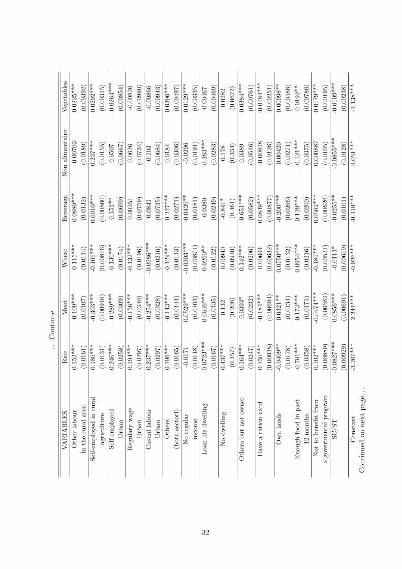
...C

onti

nue

VA

RIA

BL

ES

Ric

eM

eat

Whe

atB

ever

age

Non

alim

enta

ire

Veg

etab

les

Oth

erla

bour

0.15

2***

-0.1

09**

*-0

.115

***

-0.0

880*

**-0

.007

030.

0225

***

inth

eru

ral

area

(0.0

161)

(0.0

107)

(0.0

114)

(0.0

132)

(0.0

189)

(0.0

0392

)Se

lf-em

ploy

edin

rura

l0.

180*

**-0

.303

***

-0.1

06**

*0.

0910

***

0.23

7***

0.02

92**

*ag

ricu

ltur

e(0

.013

1)(0

.009

16)

(0.0

0816

)(0

.008

00)

(0.0

155)

(0.0

0315

)Se

lf-em

ploy

ed0.

246*

**-0

.289

***

-0.1

36**

*0.

151*

*0.

0507

-0.0

264*

**U

rban

(0.0

258)

(0.0

309)

(0.0

174)

(0.0

699)

(0.0

667)

(0.0

0854

)R

egul

ary

wag

e0.

194*

**-0

.156

***

-0.1

32**

*0.

0025

10.

0626

-0.0

0826

Urb

an(0

.029

7)(0

.034

0)(0

.019

6)(0

.075

9)(0

.073

4)(0

.009

90)

Cas

ual

labo

ur0.

237*

**-0

.254

***

-0.0

986*

**0.

0841

0.10

3-0

.008

66U

rban

(0.0

297)

(0.0

328)

(0.0

216)

(0.0

735)

(0.0

684)

(0.0

0943

)O

ther

s0.

196*

**-0

.143

***

-0.1

29**

*-0

.227

***

0.01

840.

0396

***

(bot

hse

ctor

l)(0

.016

5)(0

.014

4)(0

.011

3)(0

.027

1)(0

.030

6)(0

.004

97)

No

regu

lar

-0.0

171

0.05

29**

*-0

.030

3***

-0.0

420*

*-0

.029

60.

0129

***

inco

me

(0.0

118)

(0.0

103)

(0.0

0871

)(0

.018

1)(0

.019

1)(0

.003

35)

Loa

nhi

sdw

ellin

g-0

.072

3***

0.06

46**

*0.

0260

**-0

.038

0-0

.383

***

-0.0

0467

(0.0

167)

(0.0

135)

(0.0

122)

(0.0

249)

(0.0

283)

(0.0

0469

)N

odw

ellin

g0.

437*

**0.

132

0.00

940

-0.8

41*

0.17

80.

0282

(0.1

57)

(0.2

06)

(0.0

910)

(0.4

61)

(0.3

34)

(0.0

672)

Oth

ers

but

not

owne

r0.

164*

**0.

0393

*0.

142*

**-0

.651

***

0.03

890.

0384

***

(0.0

247)

(0.0

232)

(0.0

206)

(0.0

582)

(0.0

516)

(0.0

0761

)H

ave

ara

tion

card

0.15

0***

-0.1

84**

*0.

0069

40.

0849

***

-0.0

0828

-0.0

184*

**(0

.009

38)

(0.0

0694

)(0

.006

32)

(0.0

0877

)(0

.012

6)(0

.002

51)

Ow

nla

nds

-0.0

409*

*0.

0321

**0.

0750

***

-0.2

00**

*0.

0042

00.

0099

8**

(0.0

178)

(0.0

134)

(0.0

132)

(0.0

266)

(0.0

271)

(0.0

0486

)E

noug

hfo

odin

past

-0.7

01**

*0.

173*

**0.

0954

***

0.12

9***

-0.1

21**

*0.

0192

**12

mon

ths

(0.0

358)

(0.0

171)

(0.0

216)

(0.0

200)

(0.0

375)

(0.0

0786

)N

otto

bene

fitfr

om0.

102*

**-0

.047

4***

-0.1

89**

*0.

0562

***

0.00

0887

0.01

79**

*a

gove

rmen

tal

prog

ram

(0.0

0889

)(0

.005

82)

(0.0

0521

)(0

.006

26)

(0.0

105)

(0.0

0195

)SC

/ST

-0.0

827*

**0.

0856

***

-0.0

113*

-0.0

255*

*-0

.085

5***

-0.0

109*

**(0

.009

29)

(0.0

0691

)(0

.006

19)

(0.0

101)

(0.0

128)

(0.0

0238

)C

onst

ant

-3.2

67**

*2.

244*

**-0

.926

***

-0.4

19**

*4.

051*

**-1

.138

***

Con

tinu

edon

next

page

...

32

...C

onti

nue

VA

RIA

BL

ES

Ric

eM

eat

Whe

atB

ever

age

Non

alim

enta

ire

Veg

etab

les

(0.0

825)

(0.0

814)

(0.0

526)

(0.1

32)

(0.1

52)

(0.0

225)

R-s

quar

ed0.

263

0.30

90.

160

0.39

70.

380

0.21

2

Rob

ust

stan

dard

erro

rsin

pare

nthe

ses

***

p<0.

01,

**p<

0.05

,*

p<0.

1

Tab

le14

:R

esul

tsof

Vul

nera

bilit

yR

egre

ssio

n(N

SSD

ata)

for

som

eco

mm

odit

ies

(infl

atio

nra

te:1

0%)

33