Fomc 20050202 Text Material

Presentation Materials (6.93 MB PDF)

Pages 137 to 177 of the Transcript

Appendix 1: Materials used by Messrs. Wilcox, Elmendorf, and Reinhart

Material for Board Staff Presentation on:Considerations Pertaining to the Establishment of a Specific, Numerical, Price-RelatedObjective for Monetary PolicyDivisions of Research & Statistics and Monetary AffairsFebruary 1, 2005

RESTRICTED CONTROLLED (FR) CLASS I (FOMC)

Exhibit 1A Specific, Numerical, Price-Related Objective for Monetary Policy?

Top panelInflation Rates

A time-series plot of three measures of inflation: the GDP chain price index, the PCE chain priceindex, and the CPI current methods index. All three indexes are shown in the form of four-quarterpercent changes. The plot begins in 1950 and ends in 2004. The chart shows that the three seriesfollowed a similar pattern. All three show a burst of inflation in the early 1950s. Inflation was lowand stable during the first half of the 1960s but then increased sharply and was very volatile throughthe early 1980s. Beginning in the early 1980s, inflation generally trended downward. From the early1990s through the end of the sample period, inflation was low and stable by historical standards,fluctuating in the neighborhood of 2 percent.

Middle panelKey characteristics of a specific, numerical, price-related objective:

Numerical rather than qualitative;Stated in terms of a particular published index; andEither inflation control or price-level control.

Bottom panelA premise of the paper:

A price objective should be chosen to minimize the costs of deviations from price stability.The premise suggests that the objective should be defined with respect to the price index mostclosely related to such costs.

Exhibit 2Potential Benefits and Costs of Adopting a Specific Price-Related Objective

Top panelPotential Benefits:

Could help preserve the present commitment to price stability.Could better anchor long-run inflation expectations and thereby reduce the volatility of bothinflation and real activity.Could improve public understanding of monetary policy.Could help focus policy debates within the FOMC.

Middle panelPotential Costs:

Could mislead the public into believing that emphasis had shifted toward the price objective.Could cause the FOMC inadvertently to place more emphasis on the price objective.Could diminish the FOMC's credibility when inflation differed from the stated objective.Could constrain future actions of the FOMC in an unhelpful manner.

Bottom panelEmpirical Evidence:

Little to no evidence regarding the likely influence on FOMC decision-making or the qualityof communications with the public.Some hints from foreign experience that specific price objectives have helped anchorlong-term inflation expectations.Disputed evidence that the reduced volatility of inflation and real output owes to improvedconduct of U.S. monetary policy.Simulation-based evidence that better-anchored inflation expectations would reduce thevolatility of inflation and real output.

Exhibit 3Operational Issues Related to Specifying a Numerical Price-Related Objective

Top-left panelA checklist for policymakers:

Which price index?The inflation rate or the price level?What average rate?Point objective or range?

Top-right panelFor index, we favor consumer prices on the grounds of:

Familiarity.Quality of measurement.

Empirical result that inflation rates move together in the long run.

Middle panelIf an inflation objective, at what rate?

Measurement bias: Nearly 1 percentage point for CPI; about ½ percentage point for PCEprices.Rationales for aiming for zero true inflation: Traditional costs of inflation.Rationales for aiming for positive true inflation: Downward nominal wage rigidity; zero lowerbound on nominal interest rates.

Bottom panelEffect of zero lower bound under an updated Taylor rule:

Target PCE inflation rate(measured rate, with bias-adjusted rate in parentheses)

½ (0) 1½ (1) 2½ (2)

Fraction of time with funds rate at zero .16 .10 .06

Standard deviation of output gap* 2.53 2.31 2.21

Standard deviation of unemployment rate* 1.40 1.27 1.22

* measured in percentage points Return to table

Exhibit 4Accuracy in Achieving an Inflation Objective

Top panelImperfect controllability:

Inflation is volatile, and monetary policy influences it only indirectly and with a lag.The FOMC could not hit a point objective precisely or guarantee a narrow range.

Middle panelPercent of time that PCE inflation averaged over four quarters could be held within ± 1percentage point of desired rate:

Total Core

Volatility of economic shocks matters:

1. Drawn from 1968 to 2004 experience 59 64

2. Drawn from 1984 to 2004 experience 68 73

Expectations formation matters:

3. VAR-based expectations with imperfect credibility 68 73

4. VAR-based expectations with perfect credibility 80 89

Bottom panelSummary:

The FOMC could likely keep four-quarter total PCE inflation within a ± 1-percentage-pointband about 2/3 to 3/4 of the time.

Exhibit 5Governance Issues Related to the Specification of Price Stability

A decision tree with five steps.

Step 1

[text box] Is an explicit numerical specification of price stability helpful? (YES or NO)

Step 2

NO YES

[text box with blue border] Continue the status quo.

At the margin, the FOMC could:

encourage participants to be more specific aboutpreferences;use the minutes, testimonies, and the MPR toprovide additional guidance to the public.

[Stop]

[text box] Should the objective be made public? (YES orNO)

Step 3

NO YES

[text box with red border] Agreement on a private objectivemay facilitate internal communications, but

how can the FOMC justify keeping it secret?how will the FOMC keep it secret?

[Stop]

[text box] Should the objective be decided by the Congress(by amending the Federal Reserve Act) or by the FOMC?(CONGRESS or FOMC)

Step 4

FOMC CONGRESS

[text box] How will the FOMC choose an inflationobjective? (as a group decision or as individual decisions)

[text box with red border] Is the FOMC:

comfortable in seeking amendment to the FRA?confident that the Congress would pick anappropriate inflation objective?

And will this lead to the creation of a numerical objectivefor output growth or employment as well?

[Stop]

Step 5

As a group decision As individual decisions

[text box with blue border] As a group decision, similar tochoosing a range for a monetary aggregate.

[Stop]

[text box with blue border] As individual decisions,summarized by announcing the range and central tendencyof participants' views.[Stop]

Exhibit 6Key Questions for Today's Discussion

Top panelHow do you define price stability?

Is it known by inference about behavior or by a numerical specification?If the latter,

What price index do you prefer?Should the objective be stated in terms of a path for the price level or as the rate ofinflation?What are the desired point estimates or ranges for the inflation objective?

Bottom panelWhat role should the price objective play in the Committee's policy process?

Alternative I: Maintain the status quoPerhaps provide more information to the public over time as to your attitudes towardprevailing and prospective inflation

Alternative II: Vote formally on a numerical inflation goalAlternative III: Survey participants as to the appropriate inflation objective

Appendix 2: Materials used by Mr. Kos

Page 1

Top panel

Title: Current U.S. 3-Month Deposit Rates and Rates Implied by Traded Forward Rate AgreementsSeries: LIBOR Fixed, 3-month forward, 6-month forward, and 9-month forwardHorizon: December 1, 2004 - January 31, 2005Description: US forward rate agreements and LIBOR increased slightly.

Middle-left panel

Title: 2-Year Treasury YieldSeries: 2-Year Treasury YieldHorizon: December 1, 2004 - January 31, 2005Description: The 2-year Treasury yield has increased slightly.

Middle-right panel

Title: 10-Year Treasury YieldSeries: 10-Year Treasury YieldHorizon: December 1, 2004 - January 31, 2005Description: The 10-year Treasury yield has decreased slightly.

Bottom-left panel

Title: Yield Spread Between 2- and 10-Year Treasury NotesSeries: 2-year and 10-year Treasury NotesHorizon: December 1, 2004 - January 31, 2005Description: Treasury yield curve flattened.

Bottom-right panel

Title: Yield Spread Between 10- and 30-Year Treasury NotesSeries: 10-year and 30-year Treasury NotesHorizon: December 1, 2004 - January 31, 2005Description: Treasury yield curve flattened.

Page 2

Top-left panel

Title: 10-Year Swap SpreadSeries: 10-Year Swap SpreadHorizon: June 30, 2004 - January 28, 2005Description: 10-Year swap spread narrowed.

Top-right panel

Title: MBS SpreadsSeries: Option-Adjusted Spread of 30-year MBS IndexHorizon: June 30, 2004 - January 28, 2005Description: The MBS spread narrowed.

Source: Lehman Brothers

Middle-left panel

Title: Investment Grade Corporate Debt SpreadsSeries: Investment grade corporate index option-adjusted spreadHorizon: June 30, 2004 - January 28, 2005Description: Investment grade corporate debt spreads narrowed.

Source: Lehman Brothers

Middle-right panel

Title: High Yield and EMBI+ SpreadsSeries: High yield bond index option-adjusted spread and EMBI+ spreadHorizon: June 30, 2004 - January 28, 2005

Description: EMBI+ and high yield bond indices declined.

Source: Merrill Lynch, JP Morgan

Bottom panel

Title: Implied Swaption VolatilitySeries: 1-month volatility on 10-year swaption and 1-month volatility on 2-year swaptionHorizon: May 3, 1999 - January 28, 2005Description: Implied swaption volatility has returned to its May 1999 levels.

Page 3

Top panel

Title: Euro-Area 3-Month Deposit Rates and Rated Implied by Traded Forward Rate AgreementsSeries: LIBOR Fixed, 3-month forward, 6-month forward, and 9-month forwardHorizon: December 1, 2004 - January 31, 2005Description: Euro-area rates have remained relatively constant.

Middle-left panel

Title: Euro-Dollar Currency PairSeries: Dollar EuroHorizon: December 1, 2004 - January 31, 2005Description: The dollar appreciated against the Euro.

Middle-right panel

Title: Dollar-Yen Currency PairSeries: Yen DollarHorizon: December 1, 2004 - January 31, 2005Description: The dollar appreciated against the Yen.

Bottom-left panel

Title: Dollar-Yuan Exchange Value Implied by the NDF MarketSeries: Dollar-Yuan 1-month NDF, 6-month NDF, and 12-month NDFHorizon: July 1, 2004 - January 31, 2005Description: Implied dollar-Yuan exchange rate declined in the 6-month and 12-month terms.

Bottom-right panel

Title: Foreign Exchange Reserves of China & JapanSeries: Japanese and Chinese reservesHorizon: December 31, 2003 - December 31, 2004Description: Japanese and Chinese reserves rose.

Page 4

Top-left panel

Title: Current Account Balances (CAB) at the Bank of Japan and the Overnight Call RateSeries: CAB and Uncollateralized overnight call rateHorizon: April 30, 1998 - December 31, 2004Description: The CAB increased while the uncollateralized o/n call rate decreased.

Source: BoJ

Top-right panel

Title: Japanese Call Market Uncollateralized Amount OutstandingSeries: Yen holdingsHorizon: January 4, 1999 - January 28, 2005Description: The uncollateralized yen outstanding declined.

Middle-left panel

Title: 1-month Rolling Average of the 3-month Bill Auction HistorySeries: Issue size and Bid-to-Cover ratioHorizon: April 30, 2002 - January 19, 2005Description: The issue size and the bid-to-cover ratio increased.

Source: Ministry of Finance

Middle-right panel

Title: BoJ Securities HoldingsSeries: JGBs-outright, TB/FB-outright, Tegata bills*-outright, CP under repo, and JGS* under repoHorizon: July 31, 1996 - December 31, 2004Description: BoJ securities holdings increased.

* Source: BoJ* Tegata Bills from financial institutions incl. bills utilizing corp debt obligations* Japanese Government Securities (JGS): amount outstanding of JGBs, TBs, and FBs purchased from financialinstitutions Return to text

Bottom-left panel

Title: Bid-to-Cover on BoJ Outright Purchases of FB/TBsSeries: Bid-to-cover ratioHorizon: April 8, 2004 - January 13, 2005Description: The bid-to-cover ratio has declined.

Source: BoJ

Bottom-right panel

Title: Changes in the Japanese Government Bill Curve Since the Start of Quantitative EasingSeries: Japanese government bill curve for 3-month, 6-month, 12-month, and 2-year horizonHorizon: 3/19/2001, 1/31/2004, and 1/31/2005Description: The 3-month, 6-month, and 12-month value has decreased, while the 2-year value hasincreased.

Page 5

Top panel

Title: Daily Intra-Day Standard Deviations of the Federal Funds RateSeries: Annual average of daily values and annual medians of daily valuesHorizon: 1987-2004Description: The average and median have decreased.

Bottom panel

Title: Average Intraday Standard Deviation of Federal Funds Rates (Maintenance Period Averages)Series: Standard deviation of federal funds ratesHorizon: January 21, 2004 - January 19, 2005Description: The standard deviation has declined.

Appendix 3: Materials used by Messrs. Slifman and Struckmeyer, and Ms.Johnson

Material for Staff Presentation on the Economic OutlookFebruary 2, 2005

STRICTLY CONFIDENTIAL (FR) CLASS I-FOMC**Downgraded to Class II upon release of the February 2005 Monetary Policy Report.

Chart 1Recent Indicators

Top-left panelPrivate Payroll Employment

Average monthly change, thousands

2002 -68

2003:H1 -34

2003:H2 33

2004:H1 218

2004:Q3 93

2004:Q4 181

Top-right panelManufacturing Industrial Production

Percent change, a.r.

2002:Q1 2.78

2002:Q2 3.41

2002:Q3 2.18

2002:Q4 -3.19


2003:Q1 -0.62

2003:Q2 -3.33

2003:Q3 3.92

2003:Q4 6.50

2004:Q1 5.63

2004:Q2 6.04

2004:Q3 4.02

2004:Q4 4.15

1972-2003 average: 2.80

Middle-left panelReal PCE exc. Motor Vehicles*


2002:Q1 4.07

2002:Q2 2.82

2002:Q3 1.41

2002:Q4 3.43

2003:Q1 3.17

2003:Q2 2.81

2003:Q3 4.55

2003:Q4 3.91

2004:Q1 4.78

2004:Q2 2.02

2004:Q3 3.92

2004:Q4 4.84

* In this and subsequent charts, NIPA series in 2004:Q4 are from the January Greenbook. Return to text

Middle-right panelSales of Light Vehicles

Millions of units, a.r.

Jan 2002 16.22

Feb 2002 17.00

Mar 2002 16.78

Apr 2002 17.34

May 2002 15.84

Jun 2002 16.63

Jul 2002 17.83

Millions of units, a.r.

Aug 2002 18.10

Sep 2002 16.32

Oct 2002 15.93

Nov 2002 16.20

Dec 2002 17.60

Jan 2003 16.42

Feb 2003 15.84

Mar 2003 16.21

Apr 2003 16.43

May 2003 16.15

Jun 2003 16.69

Jul 2003 16.78

Aug 2003 17.93

Sep 2003 16.95

Oct 2003 16.14

Nov 2003 17.20

Dec 2003 16.99

Jan 2004 16.30

Feb 2004 16.63

Mar 2004 16.84

Apr 2004 16.49

May 2004 17.76

Jun 2004 15.76

Jul 2004 16.87

Aug 2004 16.71

Sep 2004 17.43

Oct 2004 16.9

Nov 2004 16.3

Dec 2004 18.3

Bottom-left panel

Title: Orders and Shipments of Nondefense Capital Goods (excluding aircraft)Series: Orders and ShipmentsHorizon: 2002 to 2004Description: The data are plotted on two curves and represent the three-month moving average.Units are billions of dollars.

The curve for shipments starts in 2002:Q1 at about 53, followed by an increase to just above 53. Thecurve then dips to about 53 through 2002:Q2 and increases to just above 53 in 2002:Q3. The curve

decreases to about 52 by 2003:Q2, after which it moves generally upward until reaching about 63 inDecember 2004.

The curve for orders starts at nearly 53 in 2002:Q1; it decreases to about 52 in 2002:Q2, increases tojust below 53 through 2002:Q3, and dips to about 51 by year-end. In 2003:Q1, the curve increases tojust above 53, then continues upward to about 58 by year-end. The curve decreases to about 57 in2004:Q1; it then climbs to about 61 in 2004:Q2, dips to a little under 61 in 2004:Q3, increases to alittle above 63 in the middle of 2004:Q4, then decreases to end at about 63 in December 2004.

An inset box shows the December percent change at 2.2 percent for shipments and 1.8 percent fororders.

Bottom-right panelReal GDP


2004:Q4

Jan. GB BEA

1. Real GDP 3.5 3.1

Contributions (percentage points)

2. Final sales 2.7 2.7

3. Inventories .8 .4

Chart 2Overview

Top panelKey Background Factors

Monetary policy: We assume a continuing withdrawal of monetary accommodation over thenext two years. The federal funds rate reaches 3 percent in the fourth quarter of this year and3-½ percent in the latter part of 2006 -- a path quite similar to that implied by futures quotes.Fiscal policy: FI is expected to be neutral in 2005 and provide only a small positive impetus toGDP growth in 2006.Oil prices: We continue to be guided in our forecast by futures markets, which expect prices todrift down over the next two years.Dollar: The foreign exchange value of the dollar is expected to drift down.Stock market: Prices are assumed to rise 6-½ percent per year, which would roughly maintainrisk-adjusted parity with the yield on long-term bonds.House prices: The rate of increase is expected to slow from last year's torrid pace.

Bottom panelReal Gross Domestic Product

Percent change, Q4/Q4

2004 2005 2006

2004 2005 2006

1. GDP 3.8 3.9 3.6

Contribution from: Percentage points

2. Private consumption and fixed investment 4.1 3.4 3.5

3. Imports -1.4 -.8 -1.2

4. Exports .5 .9 .7

5. Government .2 .6 .5

6. Inventory investment .4 -.2 .1

Chart 3What Keeps Growth Above Potential Through 2006?

Top panel

Monetary policy: The real fed funds rate is projected to still be below its long-run averageover the projection period and on the stimulative side of the short-run measures of r-star shownin the Bluebook.Other financial market conditions:

Nominal long-term rates are projected to be little changed, despite the assumed rise inshort-term rates.Corporate balance sheets are quite strong: Cash is abundant and interest expensesrelative to cash flow are at low levels.Defaults, delinquencies and risk spreads are quite low.Banks continue to ease lending standards.

Oil prices: Higher oil prices reduced GDP growth ¾ percentage point in 2004. The negativeeffects wane to -¼ percentage point in 2005 as oil prices begin to recede; the projected declinein prices boosts GDP growth slightly in 2006.

Middle-left panelReal Federal Funds Rate*

Percent Forecast

1990:Q1 4.44 ND

1990:Q2 3.95 ND

1990:Q3 3.63 ND

1990:Q4 3.35 ND

1991:Q1 2.08 ND

1991:Q2 2.09 ND

1991:Q3 1.92 ND

1991:Q4 1.00 ND

1992:Q1 0.38 ND

1992:Q2 0.19 ND

Percent Forecast

1992:Q3 -0.07 ND

1992:Q4 -0.04 ND

1993:Q1 0.34 ND

1993:Q2 0.26 ND

1993:Q3 0.56 ND

1993:Q4 0.70 ND

1994:Q1 1.01 ND

1994:Q2 1.82 ND

1994:Q3 2.03 ND

1994:Q4 2.71 ND

1995:Q1 3.34 ND

1995:Q2 3.67 ND

1995:Q3 3.74 ND

1995:Q4 3.66 ND

1996:Q1 3.35 ND

1996:Q2 3.37 ND

1996:Q3 3.52 ND

1996:Q4 3.44 ND

1997:Q1 3.52 ND

1997:Q2 3.75 ND

1997:Q3 3.96 ND

1997:Q4 4.15 ND

1998:Q1 4.19 ND

1998:Q2 4.34 ND

1998:Q3 4.22 ND

1998:Q4 3.43 ND

1999:Q1 3.35 ND

1999:Q2 3.22 ND

1999:Q3 3.58 ND

1999:Q4 3.76 ND

2000:Q1 3.82 ND

2000:Q2 4.53 ND

2000:Q3 4.90 ND

2000:Q4 4.94 ND

2001:Q1 3.97 ND

2001:Q2 2.51 ND

2001:Q3 1.54 ND

Percent Forecast

2001:Q4 -0.09 ND

2002:Q1 -0.09 ND

2002:Q2 -0.05 ND

2002:Q3 -0.19 ND

2002:Q4 -0.07 ND

2003:Q1 -0.33 ND

2003:Q2 -0.12 ND

2003:Q3 -0.09 ND

2003:Q4 -0.21 ND

2004:Q1 -0.37 ND

2004:Q2 -0.50 ND

2004:Q3 -0.07 ND

2004:Q4 0.44 ND

2005:Q1 ND 1.06

2005:Q2 ND 1.42

2005:Q3 ND 1.23

2005:Q4 ND 1.44

2006:Q1 ND 1.69

2006:Q2 ND 1.75

2006:Q3 ND 2.06

2006:Q4 ND 2.10

40-year average: 2.60

* Nominal federal funds rate less the percent change in the core PCE price index over the previous four quarters. Return totext

Middle-right panel

Title: Interest Expense to Cash FlowSeries: Interest expense to cash flowHorizon: 1990 to 2006Description: Data are plotted as a curve. Unit is percent. A forecast is provided for 2005 and 2006.

The curve begins in 1990 at about 20.75, dips to about 20 by the end of the year, increases to about20.75 in early 1991 and then falls to about 17 by year-end. It then decreases to about 13 in 1992 andincreases to about 13.5 in 1993. The curve decreases to about 11 in 1994, increases to just above 12in 1995, then drops to about 10 in 1996 and 1997. The curve then continues generally upward toabout 17 by 2002, after which it generally decreases through 2004 to end at about 11.

The curve then shows a forecast from 2005 through 2006, where it increases to about 12.

Source: Flow of Funds.

Bottom-left panelBank Lending Standards for C&I Loans

Net percent*

1990:Q2 56.90

1990:Q3 39.45

1990:Q4 48.90

1991:Q1 36.00

1991:Q2 15.50

1991:Q3 12.25

1991:Q4 9.00

1992:Q1 5.25

1992:Q2 0.90

1992:Q3 -1.70

1992:Q4 4.35

1993:Q1 2.65

1993:Q2 -7.85

1993:Q3 -19.45

1993:Q4 -17.75

1994:Q1 -12.95

1994:Q2 -12.20

1994:Q3 -6.95

1994:Q4 -17.40

1995:Q1 -6.85

1995:Q2 -5.90

1995:Q3 -6.05

1995:Q4 -3.45

1996:Q1 6.95

1996:Q2 -0.90

1996:Q3 -3.70

1996:Q4 -7.80

1997:Q1 -5.45

1997:Q2 -6.95

1997:Q3 -5.70

1997:Q4 -7.00

1998:Q1 1.80

1998:Q2 -7.10

1998:Q3 0.00

1998:Q4 36.40

1999:Q1 7.40

1999:Q2 10.00

Net percent*

1999:Q3 5.40

1999:Q4 9.10

2000:Q1 10.90

2000:Q2 24.60

2000:Q3 33.90

2000:Q4 43.80

2001:Q1 59.70

2001:Q2 50.90

2001:Q3 40.40

2001:Q4 50.90

2002:Q1 45.40

2002:Q2 25.00

2002:Q3 21.40

2002:Q4 20.00

2003:Q1 22.00

2003:Q2 8.90

2003:Q3 3.50

2003:Q4 0.00

2004:Q1 -17.90

2004:Q2 -23.20

2004:Q3 -20.00

2004:Q4 -21.10

2005:Q1 -23.60

* Percentage of banks reporting tighter standards less percentage of banks reporting easier standards. Return to table

Source: Sr. Loan Officer Survey.

Bottom-right panelCrude Oil Prices - WTI

Quarterly average

Dollars per barrel Forecast

2003:Q4 31.14 ND

2004:Q1 35.35 ND

2004:Q2 38.31 ND

2004:Q3 43.91 ND

2004:Q4 48.31 ND

2005:Q1 ND 47.87

2005:Q2 ND 48.33

Dollars per barrel Forecast

2005:Q3 ND 47.26

2005:Q4 ND 46.26

2006:Q1 ND 45.31

2006:Q2 ND 44.48

2006:Q3 ND 43.80

2006:Q4 ND 43.19

Chart 4Household Sector

Top-left panelReal PCE and DPI


DPI PCE DPI Forecast PCE Forecast

2003 3.9 3.8 ND ND

2004* 2.6 3.9 ND ND

2005 ND ND 4.5 3.8

2006 ND ND 4.7 3.7

* Excluding Microsoft dividend in 2004:Q4. Return to table

Top-right panelFinancial Obligations Ratio

Percent of DPI Forecast

1980:Q1 15.79 ND

1980:Q2 15.91 ND

1980:Q3 15.61 ND

1980:Q4 15.26 ND

1981:Q1 15.34 ND

1981:Q2 15.52 ND

1981:Q3 15.35 ND

1981:Q4 15.45 ND

1982:Q1 15.56 ND

1982:Q2 15.61 ND

1982:Q3 15.53 ND

1982:Q4 15.53 ND

1983:Q1 15.49 ND


1983:Q2 15.49 ND

1983:Q3 15.47 ND

1983:Q4 15.49 ND

1984:Q1 15.44 ND

1984:Q2 15.54 ND

1984:Q3 15.64 ND

1984:Q4 15.84 ND

1985:Q1 16.24 ND

1985:Q2 16.33 ND

1985:Q3 16.83 ND

1985:Q4 16.99 ND

1986:Q1 16.99 ND

1986:Q2 17.14 ND

1986:Q3 17.33 ND

1986:Q4 17.56 ND

1987:Q1 17.47 ND

1987:Q2 17.72 ND

1987:Q3 17.54 ND

1987:Q4 17.35 ND

1988:Q1 17.25 ND

1988:Q2 17.20 ND

1988:Q3 17.13 ND

1988:Q4 16.98 ND

1989:Q1 16.88 ND

1989:Q2 17.09 ND

1989:Q3 17.21 ND

1989:Q4 17.25 ND

1990:Q1 17.17 ND

1990:Q2 17.17 ND

1990:Q3 17.19 ND

1990:Q4 17.26 ND

1991:Q1 17.26 ND

1991:Q2 17.13 ND

1991:Q3 17.05 ND

1991:Q4 16.86 ND

1992:Q1 16.57 ND

1992:Q2 16.43 ND


1992:Q3 16.28 ND

1992:Q4 16.05 ND

1993:Q1 16.36 ND

1993:Q2 16.11 ND

1993:Q3 16.21 ND

1993:Q4 16.09 ND

1994:Q1 16.39 ND

1994:Q2 16.35 ND

1994:Q3 16.46 ND

1994:Q4 16.53 ND

1995:Q1 16.76 ND

1995:Q2 17.01 ND

1995:Q3 17.15 ND

1995:Q4 17.24 ND

1996:Q1 17.23 ND

1996:Q2 17.24 ND

1996:Q3 17.31 ND

1996:Q4 17.40 ND

1997:Q1 17.37 ND

1997:Q2 17.42 ND

1997:Q3 17.43 ND

1997:Q4 17.35 ND

1998:Q1 17.15 ND

1998:Q2 17.16 ND

1998:Q3 17.13 ND

1998:Q4 17.18 ND

1999:Q1 17.30 ND

1999:Q2 17.48 ND

1999:Q3 17.61 ND

1999:Q4 17.53 ND

2000:Q1 17.34 ND

2000:Q2 17.47 ND

2000:Q3 17.59 ND

2000:Q4 17.87 ND

2001:Q1 17.93 ND

2001:Q2 18.18 ND

2001:Q3 17.98 ND


2001:Q4 18.48 ND

2002:Q1 18.22 ND

2002:Q2 18.22 ND

2002:Q3 18.37 ND

2002:Q4 18.40 ND

2003:Q1 18.38 ND

2003:Q2 18.23 ND

2003:Q3 18.05 ND

2003:Q4 18.06 ND

2004:Q1 18.27 ND

2004:Q2 18.17 ND

2004:Q3 18.31 ND

2004:Q4 18.11 ND

2005:Q1 ND 18.27

2005:Q2 ND 18.27

2005:Q3 ND 18.26

2005:Q4 ND 18.24

2006:Q1 ND 18.19

2006:Q2 ND 18.17

2006:Q3 ND 18.15

2006:Q4 ND 18.13

Middle-left panelHousehold Net Worth to DPI

Ratio Forecast Real estate slump scenario

1975:Q1 4.23 ND ND

1975:Q2 4.20 ND ND

1975:Q3 4.14 ND ND

1975:Q4 4.16 ND ND

1976:Q1 4.22 ND ND

1976:Q2 4.29 ND ND

1976:Q3 4.26 ND ND

1976:Q4 4.29 ND ND

1977:Q1 4.27 ND ND

1977:Q2 4.29 ND ND

1977:Q3 4.25 ND ND

1977:Q4 4.19 ND ND


1978:Q1 4.19 ND ND

1978:Q2 4.22 ND ND

1978:Q3 4.27 ND ND

1978:Q4 4.25 ND ND

1979:Q1 4.30 ND ND

1979:Q2 4.37 ND ND

1979:Q3 4.40 ND ND

1979:Q4 4.38 ND ND

1980:Q1 4.31 ND ND

1980:Q2 4.47 ND ND

1980:Q3 4.51 ND ND

1980:Q4 4.45 ND ND

1981:Q1 4.44 ND ND

1981:Q2 4.48 ND ND

1981:Q3 4.32 ND ND

1981:Q4 4.36 ND ND

1982:Q1 4.35 ND ND

1982:Q2 4.33 ND ND

1982:Q3 4.34 ND ND

1982:Q4 4.40 ND ND

1983:Q1 4.47 ND ND

1983:Q2 4.52 ND ND

1983:Q3 4.44 ND ND

1983:Q4 4.33 ND ND

1984:Q1 4.25 ND ND

1984:Q2 4.20 ND ND

1984:Q3 4.21 ND ND

1984:Q4 4.22 ND ND

1985:Q1 4.32 ND ND

1985:Q2 4.31 ND ND

1985:Q3 4.35 ND ND

1985:Q4 4.46 ND ND

1986:Q1 4.54 ND ND

1986:Q2 4.61 ND ND

1986:Q3 4.57 ND ND

1986:Q4 4.68 ND ND

1987:Q1 4.82 ND ND


1987:Q2 4.93 ND ND

1987:Q3 4.91 ND ND

1987:Q4 4.67 ND ND

1988:Q1 4.70 ND ND

1988:Q2 4.73 ND ND

1988:Q3 4.69 ND ND

1988:Q4 4.71 ND ND

1989:Q1 4.70 ND ND

1989:Q2 4.77 ND ND

1989:Q3 4.86 ND ND

1989:Q4 4.85 ND ND

1990:Q1 4.73 ND ND

1990:Q2 4.73 ND ND

1990:Q3 4.58 ND ND

1990:Q4 4.65 ND ND

1991:Q1 4.77 ND ND

1991:Q2 4.72 ND ND

1991:Q3 4.74 ND ND

1991:Q4 4.80 ND ND

1992:Q1 4.70 ND ND

1992:Q2 4.65 ND ND

1992:Q3 4.65 ND ND

1992:Q4 4.68 ND ND

1993:Q1 4.80 ND ND

1993:Q2 4.75 ND ND

1993:Q3 4.81 ND ND

1993:Q4 4.79 ND ND

1994:Q1 4.79 ND ND

1994:Q2 4.71 ND ND

1994:Q3 4.72 ND ND

1994:Q4 4.66 ND ND

1995:Q1 4.73 ND ND

1995:Q2 4.85 ND ND

1995:Q3 4.96 ND ND

1995:Q4 5.03 ND ND

1996:Q1 5.06 ND ND

1996:Q2 5.09 ND ND


1996:Q3 5.09 ND ND

1996:Q4 5.20 ND ND

1997:Q1 5.16 ND ND

1997:Q2 5.41 ND ND

1997:Q3 5.53 ND ND

1997:Q4 5.54 ND ND

1998:Q1 5.72 ND ND

1998:Q2 5.73 ND ND

1998:Q3 5.43 ND ND

1998:Q4 5.74 ND ND

1999:Q1 5.79 ND ND

1999:Q2 5.94 ND ND

1999:Q3 5.80 ND ND

1999:Q4 6.19 ND ND

2000:Q1 6.14 ND ND

2000:Q2 6.02 ND ND

2000:Q3 5.95 ND ND

2000:Q4 5.75 ND ND

2001:Q1 5.47 ND ND

2001:Q2 5.61 ND ND

2001:Q3 5.21 ND ND

2001:Q4 5.48 ND ND

2002:Q1 5.38 ND ND

2002:Q2 5.14 ND ND

2002:Q3 4.94 ND ND

2002:Q4 5.04 ND ND

2003:Q1 4.97 ND ND

2003:Q2 5.14 ND ND

2003:Q3 5.14 ND ND

2003:Q4 5.37 ND ND

2004:Q1 5.37 ND ND

2004:Q2 5.39 ND ND

2004:Q3 5.42 ND ND

2004:Q4 ND 5.49 5.49

2005:Q1 ND 5.48 5.43

2005:Q2 ND 5.48 5.38

2005:Q3 ND 5.46 5.33


2005:Q4 ND 5.44 5.27

2006:Q1 ND 5.41 5.20

2006:Q2 ND 5.40 5.15

2006:Q3 ND 5.38 5.10

2006:Q4 ND 5.37 5.05

Middle-right panelHouse Prices*

Four-quarter percent change Forecast Real estate slump scenario

1976:Q1 4.17 ND ND

1976:Q2 5.61 ND ND

1976:Q3 7.45 ND ND

1976:Q4 7.49 ND ND

1977:Q1 9.03 ND ND

1977:Q2 9.90 ND ND

1977:Q3 11.62 ND ND

1977:Q4 13.22 ND ND

1978:Q1 13.40 ND ND

1978:Q2 13.05 ND ND

1978:Q3 13.52 ND ND

1978:Q4 13.27 ND ND

1979:Q1 14.91 ND ND

1979:Q2 14.05 ND ND

1979:Q3 13.14 ND ND

1979:Q4 12.02 ND ND

1980:Q1 9.16 ND ND

1980:Q2 7.43 ND ND

1980:Q3 8.52 ND ND

1980:Q4 6.94 ND ND

1981:Q1 5.87 ND ND

1981:Q2 6.63 ND ND

1981:Q3 4.67 ND ND

1981:Q4 4.37 ND ND

1982:Q1 4.85 ND ND

1982:Q2 3.46 ND ND

1982:Q3 1.61 ND ND

1982:Q4 2.21 ND ND


1983:Q1 2.75 ND ND

1983:Q2 3.39 ND ND

1983:Q3 4.62 ND ND

1983:Q4 4.25 ND ND

1984:Q1 3.89 ND ND

1984:Q2 4.43 ND ND

1984:Q3 4.76 ND ND

1984:Q4 5.36 ND ND

1985:Q1 5.29 ND ND

1985:Q2 5.35 ND ND

1985:Q3 6.25 ND ND

1985:Q4 6.67 ND ND

1986:Q1 7.18 ND ND

1986:Q2 7.71 ND ND

1986:Q3 7.80 ND ND

1986:Q4 8.27 ND ND

1987:Q1 8.53 ND ND

1987:Q2 8.18 ND ND

1987:Q3 7.88 ND ND

1987:Q4 6.87 ND ND

1988:Q1 6.43 ND ND

1988:Q2 6.68 ND ND

1988:Q3 6.03 ND ND

1988:Q4 6.19 ND ND

1989:Q1 5.73 ND ND

1989:Q2 4.89 ND ND

1989:Q3 6.15 ND ND

1989:Q4 6.02 ND ND

1990:Q1 5.05 ND ND

1990:Q2 3.59 ND ND

1990:Q3 1.63 ND ND

1990:Q4 0.20 ND ND

1991:Q1 0.54 ND ND

1991:Q2 1.02 ND ND

1991:Q3 0.69 ND ND

1991:Q4 2.53 ND ND

1992:Q1 2.45 ND ND


1992:Q2 1.78 ND ND

1992:Q3 2.80 ND ND

1992:Q4 1.85 ND ND

1993:Q1 1.01 ND ND

1993:Q2 2.08 ND ND

1993:Q3 1.67 ND ND

1993:Q4 2.02 ND ND

1994:Q1 2.66 ND ND

1994:Q2 2.13 ND ND

1994:Q3 1.78 ND ND

1994:Q4 0.76 ND ND

1995:Q1 0.67 ND ND

1995:Q2 2.09 ND ND

1995:Q3 3.42 ND ND

1995:Q4 4.50 ND ND

1996:Q1 5.38 ND ND

1996:Q2 3.68 ND ND

1996:Q3 2.49 ND ND

1996:Q4 2.58 ND ND

1997:Q1 2.26 ND ND

1997:Q2 3.00 ND ND

1997:Q3 4.14 ND ND

1997:Q4 4.59 ND ND

1998:Q1 5.23 ND ND

1998:Q2 5.21 ND ND

1998:Q3 5.10 ND ND

1998:Q4 4.98 ND ND

1999:Q1 4.49 ND ND

1999:Q2 5.07 ND ND

1999:Q3 5.31 ND ND

1999:Q4 5.26 ND ND

2000:Q1 6.33 ND ND

2000:Q2 6.71 ND ND

2000:Q3 7.09 ND ND

2000:Q4 7.61 ND ND

2001:Q1 8.12 ND ND

2001:Q2 8.22 ND ND


2001:Q3 7.92 ND ND

2001:Q4 7.54 ND ND

2002:Q1 6.62 ND ND

2002:Q2 6.71 ND ND

2002:Q3 7.24 ND ND

2002:Q4 7.58 ND ND

2003:Q1 7.23 ND ND

2003:Q2 6.54 ND ND

2003:Q3 6.03 ND ND

2003:Q4 8.24 ND ND

2004:Q1 8.41 ND ND

2004:Q2 9.81 ND ND

2004:Q3 12.97 ND ND

2004:Q4 ND 10.95 10.95

2005:Q1 ND 11.21 8.10

2005:Q2 ND 10.00 4.00

2005:Q3 ND 6.46 -2.10

2005:Q4 ND 5.55 -5.60

2006:Q1 ND 4.71 -6.30

2006:Q2 ND 4.12 -6.90

2006:Q3 ND 3.67 -7.30

2006:Q4 ND 3.42 -7.50

* OFHEO Repeat Sales Price Index. Return to text

Bottom-left panelSingle-family Housing Starts

Millions of units, a.r. Forecast

1975:Q1 0.73 ND

1975:Q2 0.85 ND

1975:Q3 0.95 ND

1975:Q4 1.03 ND

1976:Q1 1.14 ND

1976:Q2 1.10 ND

1976:Q3 1.18 ND

1976:Q4 1.25 ND

1977:Q1 1.36 ND

1977:Q2 1.43 ND


1977:Q3 1.46 ND

1977:Q4 1.51 ND

1978:Q1 1.31 ND

1978:Q2 1.49 ND

1978:Q3 1.42 ND

1978:Q4 1.46 ND

1979:Q1 1.16 ND

1979:Q2 1.29 ND

1979:Q3 1.20 ND

1979:Q4 1.03 ND

1980:Q1 0.79 ND

1980:Q2 0.69 ND

1980:Q3 0.96 ND

1980:Q4 0.98 ND

1981:Q1 0.87 ND

1981:Q2 0.79 ND

1981:Q3 0.65 ND

1981:Q4 0.54 ND

1982:Q1 0.57 ND

1982:Q2 0.60 ND

1982:Q3 0.66 ND

1982:Q4 0.82 ND

1983:Q1 1.03 ND

1983:Q2 1.09 ND

1983:Q3 1.09 ND

1983:Q4 1.05 ND

1984:Q1 1.22 ND

1984:Q2 1.10 ND

1984:Q3 1.00 ND

1984:Q4 1.07 ND

1985:Q1 1.06 ND

1985:Q2 1.05 ND

1985:Q3 1.06 ND

1985:Q4 1.11 ND

1986:Q1 1.20 ND

1986:Q2 1.22 ND

1986:Q3 1.16 ND


1986:Q4 1.16 ND

1987:Q1 1.24 ND

1987:Q2 1.14 ND

1987:Q3 1.16 ND

1987:Q4 1.08 ND

1988:Q1 1.06 ND

1988:Q2 1.07 ND

1988:Q3 1.07 ND

1988:Q4 1.14 ND

1989:Q1 1.04 ND

1989:Q2 1.00 ND

1989:Q3 1.00 ND

1989:Q4 0.99 ND

1990:Q1 1.06 ND

1990:Q2 0.90 ND

1990:Q3 0.86 ND

1990:Q4 0.79 ND

1991:Q1 0.70 ND

1991:Q2 0.84 ND

1991:Q3 0.88 ND

1991:Q4 0.91 ND

1992:Q1 1.04 ND

1992:Q2 0.99 ND

1992:Q3 1.02 ND

1992:Q4 1.08 ND

1993:Q1 1.04 ND

1993:Q2 1.11 ND

1993:Q3 1.13 ND

1993:Q4 1.25 ND

1994:Q1 1.19 ND

1994:Q2 1.21 ND

1994:Q3 1.19 ND

1994:Q4 1.16 ND

1995:Q1 1.04 ND

1995:Q2 1.02 ND

1995:Q3 1.12 ND

1995:Q4 1.14 ND


1996:Q1 1.15 ND

1996:Q2 1.19 ND

1996:Q3 1.18 ND

1996:Q4 1.10 ND

1997:Q1 1.14 ND

1997:Q2 1.12 ND

1997:Q3 1.15 ND

1997:Q4 1.14 ND

1998:Q1 1.23 ND

1998:Q2 1.24 ND

1998:Q3 1.28 ND

1998:Q4 1.36 ND

1999:Q1 1.34 ND

1999:Q2 1.27 ND

1999:Q3 1.29 ND

1999:Q4 1.34 ND

2000:Q1 1.28 ND

2000:Q2 1.24 ND

2000:Q3 1.19 ND

2000:Q4 1.22 ND

2001:Q1 1.26 ND

2001:Q2 1.30 ND

2001:Q3 1.28 ND

2001:Q4 1.26 ND

2002:Q1 1.36 ND

2002:Q2 1.34 ND

2002:Q3 1.34 ND

2002:Q4 1.41 ND

2003:Q1 1.41 ND

2003:Q2 1.42 ND

2003:Q3 1.52 ND

2003:Q4 1.66 ND

2004:Q1 1.57 ND

2004:Q2 1.60 ND

2004:Q3 1.63 ND

2004:Q4 ND 1.61

2005:Q1 ND 1.62


2005:Q2 ND 1.61

2005:Q3 ND 1.60

2005:Q4 ND 1.60

2006:Q1 ND 1.60

2006:Q2 ND 1.59

2006:Q3 ND 1.59

2006:Q4 ND 1.59

Bottom-right panel

Title: Weighted Average Mortgage Rate (weighted average of a 30-year fixed-rate mortgage and a1-year adjustable-rate mortgage)Series: Weighted average mortgage rateHorizon: 1975 to 2006Description: Data are plotted as a curve. Unit is percent. A forecast is provided for 2005 and 2006.

The curve begins in 1975 at about 9. It then generally rises to about 18 in 1981. The curve thenfluctuates generally downward through 2004 to end at about 5.

The forecast starts in 2005 at about 5. The curve then rises to a little above 5 by year-end 2006.

Chart 5Business Sector

Top-left panelEquipment and Software exc. Transportation


High-tech Other High-tech Forecast Other Forecast

1993-2004 17.2 4.4 ND ND

2004 15.4 10.9 ND ND

2005 ND ND 12.7 1.2

2006 ND ND 17.2 4.6

Top-right panelCapacity Utilization Rate

Manufacturing

Percent Forecast

1972:Q1 81.80 ND

1972:Q2 82.86 ND

1972:Q3 83.42 ND

1972:Q4 85.71 ND

Percent Forecast

1973:Q1 87.65 ND

1973:Q2 87.54 ND

1973:Q3 87.32 ND

1973:Q4 88.08 ND

1974:Q1 86.55 ND

1974:Q2 85.73 ND

1974:Q3 84.73 ND

1974:Q4 80.51 ND

1975:Q1 73.25 ND

1975:Q2 71.54 ND

1975:Q3 73.53 ND

1975:Q4 74.95 ND

1976:Q1 76.88 ND

1976:Q2 77.64 ND

1976:Q3 78.20 ND

1976:Q4 78.93 ND

1977:Q1 80.34 ND

1977:Q2 82.46 ND

1977:Q3 82.96 ND

1977:Q4 83.20 ND

1978:Q1 82.54 ND

1978:Q2 84.50 ND

1978:Q3 84.67 ND

1978:Q4 85.78 ND

1979:Q1 85.43 ND

1979:Q2 84.55 ND

1979:Q3 83.70 ND

1979:Q4 83.06 ND

1980:Q1 82.65 ND

1980:Q2 77.93 ND

1980:Q3 75.84 ND

1980:Q4 78.58 ND

1981:Q1 78.10 ND

1981:Q2 78.11 ND

1981:Q3 77.55 ND

1981:Q4 75.01 ND

1982:Q1 72.81 ND

Percent Forecast

1982:Q2 71.98 ND

1982:Q3 70.85 ND

1982:Q4 68.99 ND

1983:Q1 70.26 ND

1983:Q2 72.19 ND

1983:Q3 74.71 ND

1983:Q4 76.72 ND

1984:Q1 78.75 ND

1984:Q2 79.49 ND

1984:Q3 79.69 ND

1984:Q4 79.64 ND

1985:Q1 79.03 ND

1985:Q2 78.64 ND

1985:Q3 78.12 ND

1985:Q4 78.15 ND

1986:Q1 78.66 ND

1986:Q2 78.29 ND

1986:Q3 78.43 ND

1986:Q4 78.98 ND

1987:Q1 79.67 ND

1987:Q2 80.47 ND

1987:Q3 81.35 ND

1987:Q4 83.16 ND

1988:Q1 83.40 ND

1988:Q2 84.09 ND

1988:Q3 84.19 ND

1988:Q4 84.90 ND

1989:Q1 84.83 ND

1989:Q2 83.59 ND

1989:Q3 82.37 ND

1989:Q4 81.94 ND

1990:Q1 82.21 ND

1990:Q2 82.19 ND

1990:Q3 81.81 ND

1990:Q4 80.01 ND

1991:Q1 77.80 ND

1991:Q2 77.87 ND

Percent Forecast

1991:Q3 78.90 ND

1991:Q4 78.83 ND

1992:Q1 78.60 ND

1992:Q2 79.60 ND

1992:Q3 79.78 ND

1992:Q4 79.77 ND

1993:Q1 80.20 ND

1993:Q2 80.09 ND

1993:Q3 79.93 ND

1993:Q4 80.83 ND

1994:Q1 81.27 ND

1994:Q2 82.44 ND

1994:Q3 82.84 ND

1994:Q4 83.84 ND

1995:Q1 83.94 ND

1995:Q2 82.87 ND

1995:Q3 82.30 ND

1995:Q4 81.95 ND

1996:Q1 80.80 ND

1996:Q2 81.35 ND

1996:Q3 81.66 ND

1996:Q4 81.78 ND

1997:Q1 82.49 ND

1997:Q2 82.49 ND

1997:Q3 82.87 ND

1997:Q4 83.23 ND

1998:Q1 82.79 ND

1998:Q2 81.95 ND

1998:Q3 81.23 ND

1998:Q4 81.26 ND

1999:Q1 81.06 ND

1999:Q2 80.96 ND

1999:Q3 80.80 ND

1999:Q4 81.47 ND

2000:Q1 81.42 ND

2000:Q2 81.71 ND

2000:Q3 80.36 ND

Percent Forecast

2000:Q4 78.76 ND

2001:Q1 76.53 ND

2001:Q2 75.04 ND

2001:Q3 73.65 ND

2001:Q4 72.65 ND

2002:Q1 73.00 ND

2002:Q2 73.59 ND

2002:Q3 74.04 ND

2002:Q4 73.54 ND

2003:Q1 73.52 ND

2003:Q2 72.97 ND

2003:Q3 73.68 ND

2003:Q4 74.76 ND

2004:Q1 75.62 ND

2004:Q2 76.51 ND

2004:Q3 77.03 ND

2004:Q4 77.57 ND

2005:Q1 ND 78.41

2005:Q2 ND 78.81

2005:Q3 ND 79.42

2005:Q4 ND 80.08

2006:Q1 ND 80.69

2006:Q2 ND 81.11

2006:Q3 ND 81.45

2006:Q4 ND 81.78

1972-2003 average: 79.90

Middle-left panel

Title: Rate of Return on Capital for Nonfinancial Corporate Business (nonfinancial corporate profitswith IVA and CADJ plus interest, divided by nonfinancial stock of fixed assets)Series: Rate of return on capital for nonfinancial corporate businessHorizon: 1972 to 2006Description: Data are plotted as a curve. Unit is percent. A forecast is provided for 2004:Q4 through2006.

The curve starts in 1972 at about 6. It increases to about 7 in 1973, drops to about 4 in 1974, andrises to about 6 in 1975. It then fluctuates from that point between a bit below 5 and about 6.5through 1978. The curve decreases to about 3.25 in 1980, increases to about 4.75 in 1981, thendecreases to about 3.25 by 1983. The curve increases to about 5.75 in 1984, then moves generallydownward to about 4 by 1987. The curve increases to reach about 5.75 in early 1989, then fluctuates

downward through 1992 to about 4. The curve fluctuates in an upward trend to about 8 by 1998, thendecreases to about 3.25 by 2002. It then increases, reaching nearly 7 by the beginning of the forecastperiod in 2004:Q4. The curve then decreases through 2006 to end at about 6.

Middle-right panelReserve Bank Queries on Capital Spending Plans

(Percent)

Jan 2004 Jan 2005

Plan to increase spending over next 6 to 12 months 51.7 47.3

Reasons cited for increase:*

Expected sales growth 53.6 47.7

Replace IT equip. 41.1 39.9

Replace other equip. 42.3 41.5

* Percent of respondents planning to increase spending. Return to table

Bottom-left panelEquipment and Software


GB Baseline No pothole scenario GB Forecast No pothole Forecast

2004 12.78 12.78 ND ND

2005 ND ND 6.61 13.13

2006 ND ND 9.82 12.67

Bottom-right panel

Title: Price Index for Desktop ComputersSeries: Production process improvements and Technological improvementsHorizon: 1994 to 2004Description: Data are plotted as three stacked bars. Unit is percent change, annual rate. Note that thepercent changes for the first three quarters of 2004 are calculated from the latest data available. Ahorizontal line is drawn at zero. The top part of each bar denotes production process improvements,and the bottom part of each bar denotes technological improvements. The bars for each period showthe following:

1994-2002: The bar for production process improvements is from 0 to about negative 5, and the barfor technological improvements is from about negative 5 to about negative 35.

2003: The bar for production process improvements is from 0 to about negative 6, and the bar fortechnological improvements is from about negative 6 to about negative 30.

2004, first three quarters (latest data available): The bar for production process improvements is from0 to about negative 10, and the bar for technological improvements is from about negative 10 toabout negative 18.

Source: Staff estimates.

Chart 6Labor Markets

Top-left panelNonfarm Payroll Employment

Avg. monthly change, thousands Forecast

2000:H1 263.50 ND

2000:H2 79.11 ND

2001:H1 -18.44 ND

2001:H2 -212.61 ND

2002:H1 -87.06 ND

2002:H2 -23.50 ND

2003:H1 -61.67 ND

2003:H2 20.72 ND

2004:H1 187.11 ND

2004:H2 165.17 ND

2005:H1 ND 217.77

2005:H2 ND 238.63

2006:H1 ND 213.23

2006:H2 ND 198.11

Top-right panelStructural Labor Productivity


Structural MFP Capital deepening Structural MFP Forecast Capital deepening Forecast

2000 1.00 1.40 ND ND

2001 2.20 1.10 ND ND

2002 2.40 0.60 ND ND

2003 2.80 0.60 ND ND

2004 2.00 0.80 ND ND

2005 ND ND 1.60 0.90

2006 ND ND 1.50 0.90

Middle-left panelLabor Productivity

Chained (2000) dollars per hour

Actual Forecast

2000:Q1 38.37 ND

2000:Q2 39.08 ND

Actual Forecast

2000:Q3 38.98 ND

2000:Q4 39.35 ND

2001:Q1 39.32 ND

2001:Q2 39.86 ND

2001:Q3 39.99 ND

2001:Q4 40.63 ND

2002:Q1 41.31 ND

2002:Q2 41.44 ND

2002:Q3 41.88 ND

2002:Q4 42.05 ND

2003:Q1 42.45 ND

2003:Q2 43.13 ND

2003:Q3 44.07 ND

2003:Q4 44.45 ND

2004:Q1 44.82 ND

2004:Q2 45.26 ND

2004:Q3 45.45 ND

2004:Q4 ND 45.69

2005:Q1 ND 45.87

2005:Q2 ND 46.07

2005:Q3 ND 46.27

2005:Q4 ND 46.46

2006:Q1 ND 46.68

2006:Q2 ND 46.93

2006:Q3 ND 47.19

2006:Q4 ND 47.46

Middle-right panelLabor Force Participation Rate

Percent

Actual Trend Actual Forecast Trend Forecast

1980:Q1 64.21 63.59 ND ND

1980:Q2 64.08 63.67 ND ND

1980:Q3 64.03 63.75 ND ND

1980:Q4 64.00 63.83 ND ND

1981:Q1 64.28 63.91 ND ND

1981:Q2 64.41 63.99 ND ND


1981:Q3 64.01 64.08 ND ND

1981:Q4 64.11 64.16 ND ND

1982:Q1 64.11 64.24 ND ND

1982:Q2 64.35 64.32 ND ND

1982:Q3 64.41 64.40 ND ND

1982:Q4 64.47 64.48 ND ND

1983:Q1 64.12 64.56 ND ND

1983:Q2 64.26 64.65 ND ND

1983:Q3 64.62 64.73 ND ND

1983:Q4 64.47 64.81 ND ND

1984:Q1 64.41 64.89 ND ND

1984:Q2 64.83 64.97 ND ND

1984:Q3 64.84 65.05 ND ND

1984:Q4 64.89 65.13 ND ND

1985:Q1 65.15 65.22 ND ND

1985:Q2 65.12 65.30 ND ND

1985:Q3 65.14 65.38 ND ND

1985:Q4 65.35 65.46 ND ND

1986:Q1 65.43 65.54 ND ND

1986:Q2 65.65 65.62 ND ND

1986:Q3 65.79 65.70 ND ND

1986:Q4 65.81 65.79 ND ND

1987:Q1 65.85 65.87 ND ND

1987:Q2 65.99 65.95 ND ND

1987:Q3 66.04 66.03 ND ND

1987:Q4 66.17 66.11 ND ND

1988:Q1 66.22 66.19 ND ND

1988:Q2 66.21 66.27 ND ND

1988:Q3 66.41 66.36 ND ND

1988:Q4 66.58 66.44 ND ND

1989:Q1 66.81 66.52 ND ND

1989:Q2 66.90 66.60 ND ND

1989:Q3 66.94 66.60 ND ND

1989:Q4 67.02 66.60 ND ND

1990:Q1 67.03 66.60 ND ND

1990:Q2 66.85 66.60 ND ND

1990:Q3 66.78 66.60 ND ND


1990:Q4 66.70 66.60 ND ND

1991:Q1 66.56 66.60 ND ND

1991:Q2 66.57 66.60 ND ND

1991:Q3 66.38 66.60 ND ND

1991:Q4 66.38 66.60 ND ND

1992:Q1 66.59 66.60 ND ND

1992:Q2 66.84 66.60 ND ND

1992:Q3 66.88 66.60 ND ND

1992:Q4 66.56 66.60 ND ND

1993:Q1 66.46 66.60 ND ND

1993:Q2 66.61 66.60 ND ND

1993:Q3 66.61 66.60 ND ND

1993:Q4 66.58 66.60 ND ND

1994:Q1 66.41 66.60 ND ND

1994:Q2 66.31 66.60 ND ND

1994:Q3 66.36 66.60 ND ND

1994:Q4 66.55 66.60 ND ND

1995:Q1 66.56 66.60 ND ND

1995:Q2 66.44 66.60 ND ND

1995:Q3 66.42 66.60 ND ND

1995:Q4 66.33 66.60 ND ND

1996:Q1 66.33 66.60 ND ND

1996:Q2 66.50 66.60 ND ND

1996:Q3 66.65 66.60 ND ND

1996:Q4 66.80 66.60 ND ND

1997:Q1 66.83 66.60 ND ND

1997:Q2 66.89 66.60 ND ND

1997:Q3 66.92 66.60 ND ND

1997:Q4 66.86 66.60 ND ND

1998:Q1 66.98 66.60 ND ND

1998:Q2 66.90 66.60 ND ND

1998:Q3 66.94 66.60 ND ND

1998:Q4 67.04 66.60 ND ND

1999:Q1 67.08 66.60 ND ND

1999:Q2 67.01 66.60 ND ND

1999:Q3 66.99 66.60 ND ND

1999:Q4 67.03 66.60 ND ND


2000:Q1 67.29 66.60 ND ND

2000:Q2 67.17 66.60 ND ND

2000:Q3 66.89 66.60 ND ND

2000:Q4 66.92 66.60 ND ND

2001:Q1 67.15 66.60 ND ND

2001:Q2 66.76 66.60 ND ND

2001:Q3 66.65 66.60 ND ND

2001:Q4 66.70 66.60 ND ND

2002:Q1 66.58 66.60 ND ND

2002:Q2 66.64 66.60 ND ND

2002:Q3 66.56 66.60 ND ND

2002:Q4 66.36 66.60 ND ND

2003:Q1 66.28 66.60 ND ND

2003:Q2 66.37 66.60 ND ND

2003:Q3 66.06 66.60 ND ND

2003:Q4 65.99 66.60 ND ND

2004:Q1 65.98 66.60 ND ND

2004:Q2 65.92 66.60 ND ND

2004:Q3 65.93 66.60 ND ND

2004:Q4 ND ND 66.01 66.60

2005:Q1 ND ND 66.08 66.58

2005:Q2 ND ND 66.16 66.57

2005:Q3 ND ND 66.23 66.55

2005:Q4 ND ND 66.30 66.53

2006:Q1 ND ND 66.35 66.52

2006:Q2 ND ND 66.38 66.50

2006:Q3 ND ND 66.39 66.48

2006:Q4 ND ND 66.39 66.47

Trend rate of change 1980:Q1-1989:Q2: 0.5%, 1989:Q2-2004:Q3: 0%, 2004:Q3-2006:Q4: -0.1%.

Bottom-left panelUnemployment Rate

Percent Forecast

2000:Q1 4.00 ND

2000:Q2 3.90 ND

2000:Q3 4.00 ND

2000:Q4 3.90 ND

Percent Forecast

2001:Q1 4.20 ND

2001:Q2 4.40 ND

2001:Q3 4.80 ND

2001:Q4 5.50 ND

2002:Q1 5.70 ND

2002:Q2 5.80 ND

2002:Q3 5.70 ND

2002:Q4 5.90 ND

2003:Q1 5.80 ND

2003:Q2 6.10 ND

2003:Q3 6.10 ND

2003:Q4 5.90 ND

2004:Q1 5.60 ND

2004:Q2 5.60 ND

2004:Q3 5.50 ND

2004:Q4 5.43 ND

2005:Q1 ND 5.39

2005:Q2 ND 5.35

2005:Q3 ND 5.32

2005:Q4 ND 5.29

2006:Q1 ND 5.26

2006:Q2 ND 5.23

2006:Q3 ND 5.19

2006:Q4 ND 5.15

Bottom-right panelEmployment-Population Ratio

Percent Forecast

2000:Q1 64.57 ND

2000:Q2 64.52 ND

2000:Q3 64.20 ND

2000:Q4 64.31 ND

2001:Q1 64.32 ND

2001:Q2 63.84 ND

2001:Q3 63.47 ND

2001:Q4 63.03 ND

2002:Q1 62.81 ND

Percent Forecast

2002:Q2 62.78 ND

2002:Q3 62.80 ND

2002:Q4 62.52 ND

2003:Q1 62.43 ND

2003:Q2 62.35 ND

2003:Q3 62.11 ND

2003:Q4 62.22 ND

2004:Q1 62.25 ND

2004:Q2 62.29 ND

2004:Q3 62.41 ND

2004:Q4 62.42 ND

2005:Q1 ND 62.52

2005:Q2 ND 62.62

2005:Q3 ND 62.71

2005:Q4 ND 62.79

2006:Q1 ND 62.85

2006:Q2 ND 62.90

2006:Q3 ND 62.95

2006:Q4 ND 62.98

Chart 7Compensation

Top panelHourly Labor Compensation

Four-quarter percent change

Employment costindex

P&C compensationper hour

Employment cost indexForecast

P&C compensation per hourForecast

1997:Q1 2.89 2.77 ND ND

1997:Q2 2.87 2.56 ND ND

1997:Q3 3.00 2.82 ND ND

1997:Q4 3.44 4.16 ND ND

1998:Q1 3.42 5.40 ND ND

1998:Q2 3.54 6.16 ND ND

1998:Q3 3.74 6.72 ND ND

1998:Q4 3.40 5.47 ND ND

Employment costindex

P&C compensation perhour

Employment cost indexForecast

P&C compensation per hourForecast

1999:Q1 3.01 5.46 ND ND

1999:Q2 3.20 4.29 ND ND

1999:Q3 3.17 3.65 ND ND

1999:Q4 3.51 5.19 ND ND

2000:Q1 4.56 6.88 ND ND

2000:Q2 4.59 6.85 ND ND

2000:Q3 4.68 7.99 ND ND

2000:Q4 4.42 6.42 ND ND

2001:Q1 4.16 4.54 ND ND

2001:Q2 4.05 4.83 ND ND

2001:Q3 3.94 3.33 ND ND

2001:Q4 4.17 3.53 ND ND

2002:Q1 3.99 3.26 ND ND

2002:Q2 4.09 3.53 ND ND

2002:Q3 3.73 3.37 ND ND

2002:Q4 3.43 2.84 ND ND

2003:Q1 3.90 2.81 ND ND

2003:Q2 3.68 3.41 ND ND

2003:Q3 4.15 4.57 ND ND

2003:Q4 4.12 5.39 ND ND

2004:Q1 3.82 4.57 ND ND

2004:Q2 3.97 4.55 ND ND

2004:Q3 3.75 3.94 ND ND

2004:Q4 ND ND 3.99 3.96

2005:Q1 ND ND 3.98 4.39

2005:Q2 ND ND 4.03 4.02

2005:Q3 ND ND 4.22 4.19

2005:Q4 ND ND 4.25 4.17

2006:Q1 ND ND 4.22 4.27

2006:Q2 ND ND 4.20 4.23

2006:Q3 ND ND 4.18 4.20

2006:Q4 ND ND 4.15 4.17

[inset box] 2004:Q4(Percent change, a.r.)

Predicted Actual

ECI 4.1 3.0

Predicted Actual

CPH 4.4 3.6*

* Staff estimate. Return to table

Middle-left panelInflation Expectations

Percent

Michigan SRC One year ahead, median

Jan 2000 3.00

Feb 2000 2.90

Mar 2000 3.20

Apr 2000 3.20

May 2000 3.00

Jun 2000 2.90

Jul 2000 3.00

Aug 2000 2.70

Sep 2000 2.90

Oct 2000 3.20

Nov 2000 2.90

Dec 2000 2.80

Jan 2001 3.00

Feb 2001 2.80

Mar 2001 2.80

Apr 2001 3.10

May 2001 3.20

Jun 2001 3.00

Jul 2001 2.60

Aug 2001 2.70

Sep 2001 2.80

Oct 2001 1.00

Nov 2001 0.40

Dec 2001 1.80

Jan 2002 1.90

Feb 2002 2.10

Mar 2002 2.70

Apr 2002 2.80

May 2002 2.70

Jun 2002 2.70

Michigan SRC One year ahead, median

Jul 2002 2.60

Aug 2002 2.60

Sep 2002 2.50

Oct 2002 2.50

Nov 2002 2.40

Dec 2002 2.50

Jan 2003 2.50

Feb 2003 2.70

Mar 2003 3.10

Apr 2003 2.40

May 2003 2.00

Jun 2003 2.10

Jul 2003 1.70

Aug 2003 2.50

Sep 2003 2.80

Oct 2003 2.60

Nov 2003 2.70

Dec 2003 2.60

Jan 2004 2.70

Feb 2004 2.60

Mar 2004 2.90

Apr 2004 3.20

May 2004 3.30

Jun 2004 3.30

Jul 2004 3.00

Aug 2004 2.80

Sep 2004 2.80

Oct 2004 3.10

Nov 2004 2.80

Dec 2004 3.00

Jan 2005 2.90

Percent

FRB Philadelphia One-year ahead

2000:Q1 2.46

2000:Q2 2.61

2000:Q3 2.71

FRB Philadelphia One-year ahead

2000:Q4 2.67

2001:Q1 2.49

2001:Q2 2.51

2001:Q3 2.60

2001:Q4 2.15

2002:Q1 2.20

2002:Q2 2.35

2002:Q3 2.29

2002:Q4 2.19

2003:Q1 2.12

2003:Q2 2.09

2003:Q3 1.82

2003:Q4 2.12

2004:Q1 1.63

2004:Q2 2.13

2004:Q3 2.30

2004:Q4 2.26

Middle-right panelUnemployment Gap

As shown in the chart, NAIRU remained constant at 5.00 percent.

Percent

Unemployment rate Forecast

2001:Q1 4.20 ND

2001:Q2 4.40 ND

2001:Q3 4.80 ND

2001:Q4 5.50 ND

2002:Q1 5.70 ND

2002:Q2 5.80 ND

2002:Q3 5.70 ND

2002:Q4 5.90 ND

2003:Q1 5.80 ND

2003:Q2 6.10 ND

2003:Q3 6.10 ND

2003:Q4 5.90 ND

2004:Q1 5.60 ND

2004:Q2 5.60 ND

Unemployment rate Forecast

2004:Q3 5.50 ND

2004:Q4 5.43 ND

2005:Q1 ND 5.39

2005:Q2 ND 5.35

2005:Q3 ND 5.32

2005:Q4 ND 5.29

2006:Q1 ND 5.26

2006:Q2 ND 5.23

2006:Q3 ND 5.19

2006:Q4 ND 5.15

Bottom-left panelECI Wages and Salaries

Percent Change, Q4/Q4 Forecast

2002 2.70 ND

2003 3.00 ND

2004 2.89 ND

2005 ND 3.80

2006 ND 3.67

Bottom-right panelECI Benefits

Percent Change, Q4/Q4 Forecast

2002 4.70 ND

2003 6.40 ND

2004 6.90 ND

2005 ND 5.32

2006 ND 5.28

Chart 8Recent Price Developments

Top-left panel

Title: Consumer PricesSeries: CPI and PCEHorizon: 1999 to 2004Description: Data are plotted on two curves. Units are 12-month percent change.

The CPI curve begins in 1999 at about 1.6. It then moves generally upward to about 3.75 in the firstquarter of 2000, decreases to about 3, then fluctuates between about 3.5 and 3.75 until early 2001.Then the curve drops to just below 3 before increasing to about 3.75 toward midyear. The curvegenerally falls to just above 1 near the start of 2002, then fluctuates between about 1 and almost 2through year-end. The curve then increases to just above 3 in the first quarter of 2003 and falls toabout 1.75 in the fourth quarter. The curve then increases to about 3.25 by midyear 2004, drops toabout 2.5, then increases to about 3.75 toward year-end. The curve then decreases to about 3.3 at theend of 2004.

The PCE curve begins 1999 at just below 1. It then increases to about 3 at the start of 2000. Thecurve goes generally down to about 1 by the first quarter of 2002 and stays near there until midyear.The curve then increases to about 2.5 in the first half of 2003, then fluctuates downward to about1.75 by year-end. The curve then increases to about 2.5 by midyear 2004 and drops to near 2 in aboutthe third quarter. The curve then increases to about 2.75 before decreasing and ending at about 2.3 inDecember 2004.

Top-right panel

Title: PCE Energy PricesSeries: PCE energy pricesHorizon: 2001 to 2004Description: Data are plotted as seven bars; 2001, 2002, and 2003 each have one bar representing afull year, and 2004 has four bars that each represent a quarter of a year. A horizontal line is drawn atzero. Approximate values for the seven periods are as follows.


2001 -10

2002 7

2003 6

2004:Q1 26

2004:Q2 25

2004:Q3 4

2004:Q4 16

Middle-left panel

Title: PCE Food PricesSeries: PCE food pricesHorizon: 2001 to 2004Description: Data are plotted as seven bars; 2001, 2002, and 2003 each have one bar representing afull year, and 2004 has four bars that each represent a quarter of a year. Approximate values for theseven periods are as follows.


2001 3.0

2002 1.5

2003 2.5


2004:Q1 2.4

2004:Q2 3.9

2004:Q3 2.4

2004:Q4 2.5

Middle-right panel

Title: Core PCE PricesSeries: PCE and Market PCEHorizon: 1999 to 2004Description: Data are plotted as two curves. Units are 12-month percent change.

The personal consumption expenditures (PCE) curve starts at about 1.4 at the beginning of 1999,then fluctuates between approximately 1.3 and 1.7 through the end of the year. The curve increasesto about 2 near the beginning of 2000 and decreases to about 1.5 by the end of the year. It thenincreases to approximately 2.2 in about midyear 2001, drops to about 1.5 in the third quarter, andclimbs to about 2.2 in the fourth quarter. The PCE curve then generally decreases to about 1.5 bymidyear 2002, after which it increases to about 2.4 in the third quarter, and drops to approximately1.4 by the end of the year. In 2003, the curve increases to about 1.7 in the first quarter, generallydecreases to just below 1 in the third quarter, increases to about 1.4 and then falls to about 1 by theend of the year. The curve increases to about 1.6 near the second quarter of 2004, decreases slightlyto about 1.5 in the third quarter, and increases to about 1.6 in the fourth quarter. By year-end, thecurve decreases to about 1.4.

The market PCE curve begins at just above 1 at the start of 1999, then fluctuates between 0.75 and1.25 through the year to end at just above 1 by year-end. In 2000, the curve increases to about 1.5 inthe first quarter, dips to about 1.25 in the second quarter, then increases to end at about 1.5 by the endof the year. The curve moves generally upward in 2001, reaching about 1.75 by midyear; it then dipsto about 1.6 in the third quarter and increases to about 1.75 by the end of the year. The curvedecreases to about 1.5 in the first quarter of 2002, then fluctuates downward to end at about 0.9 nearthe end of 2003. In 2004, the curve increases to about 1.6 by midyear, dips to about 1.4 in the thirdquarter, then increases to about 1.8. By the end of the year, the curve decreases to end at about 1.7.

Bottom-left panelCore PCE Components

12-month percent change

2002 2003 2004

Core PCE 1.7 1.1 1.5

Market based 1.4 1.0 1.7

Goods -1.6 -2.3 0.0

Services 3.0 2.9 2.6

Nonmarket based 3.6 1.3 0.5

Bottom-right panelPPI-Intermediate Materials less Food and Energy


2001 -1.363

2002 1.209

2003 1.902

2004:Q1 6.9

2004:Q2 11.1

2004:Q3 7.8

2004:Q4 6.4

Chart 9Inflation Outlook

Top-left panelPCE Prices

Percent change, Q4/Q4 Forecast

2002 1.77 ND

2003 1.68 ND

2004 2.47 ND

2005 ND 1.35

2006 ND 1.32

Top-right panelPCE Energy Prices


2002 7.86 ND

2003 7.18 ND

2004 17.84 ND

2005 ND -3.41

2006 ND -1.24

Middle-left panelCore PCE Prices


2002 1.52 ND

2003 1.21 ND

2004 1.51 ND

2005 ND 1.56


2006 ND 1.40

Middle-right panelCore Non-fuel Import Prices

Four-quarter percent change Forecast

2002:Q1 -2.70 ND

2002:Q2 -1.95 ND

2002:Q3 -0.66 ND

2002:Q4 0.12 ND

2003:Q1 1.20 ND

2003:Q2 1.20 ND

2003:Q3 1.12 ND

2003:Q4 1.57 ND

2004:Q1 2.28 ND

2004:Q2 3.12 ND

2004:Q3 3.45 ND

2004:Q4 ND 3.81

2005:Q1 ND 3.27

2005:Q2 ND 2.41

2005:Q3 ND 1.94

2005:Q4 ND 1.16

2006:Q1 ND 0.47

2006:Q2 ND 0.31

2006:Q3 ND 0.22

2006:Q4 ND 0.17

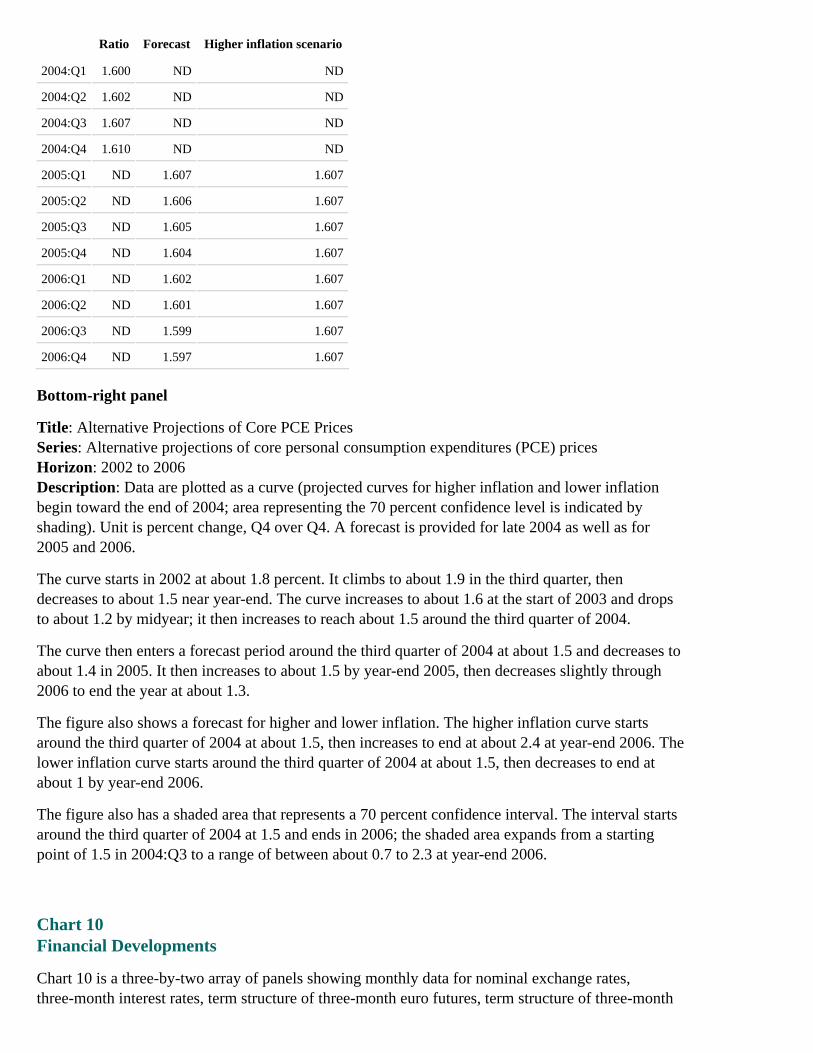
Bottom-left panelPrice Markup over Trend Unit Labor Costs

Ratio Forecast Higher inflation scenario

2002:Q1 1.572 ND ND

2002:Q2 1.578 ND ND

2002:Q3 1.589 ND ND

2002:Q4 1.602 ND ND

2003:Q1 1.603 ND ND

2003:Q2 1.597 ND ND

2003:Q3 1.590 ND ND

2003:Q4 1.588 ND ND

Ratio Forecast Higher inflation scenario

2004:Q1 1.600 ND ND

2004:Q2 1.602 ND ND

2004:Q3 1.607 ND ND

2004:Q4 1.610 ND ND

2005:Q1 ND 1.607 1.607

2005:Q2 ND 1.606 1.607

2005:Q3 ND 1.605 1.607

2005:Q4 ND 1.604 1.607

2006:Q1 ND 1.602 1.607

2006:Q2 ND 1.601 1.607

2006:Q3 ND 1.599 1.607

2006:Q4 ND 1.597 1.607

Bottom-right panel

Title: Alternative Projections of Core PCE PricesSeries: Alternative projections of core personal consumption expenditures (PCE) pricesHorizon: 2002 to 2006Description: Data are plotted as a curve (projected curves for higher inflation and lower inflationbegin toward the end of 2004; area representing the 70 percent confidence level is indicated byshading). Unit is percent change, Q4 over Q4. A forecast is provided for late 2004 as well as for2005 and 2006.

The curve starts in 2002 at about 1.8 percent. It climbs to about 1.9 in the third quarter, thendecreases to about 1.5 near year-end. The curve increases to about 1.6 at the start of 2003 and dropsto about 1.2 by midyear; it then increases to reach about 1.5 around the third quarter of 2004.

The curve then enters a forecast period around the third quarter of 2004 at about 1.5 and decreases toabout 1.4 in 2005. It then increases to about 1.5 by year-end 2005, then decreases slightly through2006 to end the year at about 1.3.

The figure also shows a forecast for higher and lower inflation. The higher inflation curve startsaround the third quarter of 2004 at about 1.5, then increases to end at about 2.4 at year-end 2006. Thelower inflation curve starts around the third quarter of 2004 at about 1.5, then decreases to end atabout 1 by year-end 2006.

The figure also has a shaded area that represents a 70 percent confidence interval. The interval startsaround the third quarter of 2004 at 1.5 and ends in 2006; the shaded area expands from a startingpoint of 1.5 in 2004:Q3 to a range of between about 0.7 to 2.3 at year-end 2006.

Chart 10Financial Developments

Chart 10 is a three-by-two array of panels showing monthly data for nominal exchange rates,three-month interest rates, term structure of three-month euro futures, term structure of three-month

yen futures, ten-year interest rates, and broad stock price indexes.

Top-left panelNominal Exchange Rates

Nominal Exchange Rates, foreign currency/U.S. dollar, for 2002 through early 2005. The range ofthe y-axis is [60, 110]; index, Jan. 2002 = 100. The three series are exchange rate indexes for majorcurrencies, the yen, and the euro. The major currencies index is the trade-weighted average againstmajor currencies. All the series begin at 100. The major currencies index rises immediately to about101, falls to about 76 by the beginning of 2004, rises to about 80 by early 2004, declines slightly toabout 78 by late 2004, falls to about 72 by end-2004, and then rises to about 74 by the end of theperiod. The exchange rate index for the yen rises immediately to about 101, falls to about 80 by thebeginning of 2004, rises to about 85 by early 2004, declines slightly to about 83 by late 2004, falls toabout 78 by end-2004, and then rises slightly to about 79 by the end of the period. The exchange rateindex for the euro rises immediately to about 102, falls to about 69 by the beginning of 2004, rises toabout 73 by early 2004, declines slightly to about 72 by late 2004, falls to about 66 by end-2004, andthen rises to about 68 by the end of the period.

Top-right panelThree-Month Interest Rates

Three-Month Interest Rates for the euro, the dollar, and the yen for 2002 through early 2005. Therange of the y-axis is [0, 4]; unit is percent. The euro rate starts at around 3-1/3 percent, increases toabout 3½ percent by mid-2002, declines to about 2¼ percent by mid-2003 and stays at about that ratethrough the end of the period. The dollar rate starts at about 1¾ percent, falls to about 1 percent bymid-2003, stays at about that rate through early 2004, and then rises to about 2¾ percent by early2005. The yen rate remains just above 0 percent throughout.

Middle-left panelTerm Structure of Three-Month Euro Futures

Term Structure of Three-Month Euro Futures as of January 27, 2004, as of June 29, 2004, and as ofFebruary 1, 2005, for 2004 through early 2007. Each series begins at the "as of" date and ends inearly 2007. The range of the y-axis is [1, 5]; unit is percent. The series as of January 27, 2004, beginsat about 2 percent and rises smoothly to about 4 percent by the end of the period. The series as ofJune 29, 2004, begins at about 2¼ percent and rises smoothly to about 4¼ percent by the end of theperiod. The series as of February 1, 2005, begins just above 2 percent and rises smoothly to about 3percent by the end of the period.

Middle-right panelTerm Structure of Three-Month Yen Futures

Term Structure of Three-Month Yen Futures as of January 27, 2004, as of June 29, 2004, and as ofFebruary 1, 2005, for 2004 through early 2007. Each series begins at the "as of" date and ends inearly 2007. The range of the y-axis is [-1, 3]; unit is percent. The series as of January 27, 2004,begins just above 0 percent, stays at about that level through 2004 and then rises smoothly to justunder 1 percent by the end of the period. The series as of June 29, 2004, begins just above 0 percent,stays at about that level through 2004 and then rises smoothly to about 1¼ percent by the end of theperiod. The series as of February 1, 2005, begins just above 0 percent and rises smoothly to about ½percent by the end of the period.

Bottom-left panel

Ten-Year Interest Rates

Ten-Year Interest Rates for Germany, the United States, and Japan for 2002 through early 2005. Therange of the y-axis is [0, 6]; unit is percent. The yields for Germany and the United States start atabout 5 percent and track fairly closely for the entire period, though they diverge a bit by early 2005.The rate for Germany rises to about 5¼ percent by early 2002, declines to about 3½ percent bymid-2003, rises to about 4¼ percent by late 2003, declines to about 3¾ percent by early 2004, risesto about 4¼ percent by mid-2004, and then declines to about 3½ percent by the end of the period.The rate for the United States rises to about 5-1/3 percent by early 2002, declines to about 3¼percent by mid-2003, quickly rises to about 4½ percent, declines to about 3¾ percent by early 2004,rises to about 4¾ percent by mid-2004, and then declines to just above 4 percent by the end of theperiod. The rate for Japan starts at about 1½ percent, declines to about ½ percent by mid-2003, risesto about 1¾ percent by mid-2004, and then declines to about 1¼ percent by the end of the period.

Bottom-right panelBroad Stock Price Indexes

Broad Stock Price Indexes for TOPIX, the S&P 500, and the DJ Euro Stoxx indexes for 2002through early 2005. The range of the y-axis is [50, 130]; index, Jan. 2002 = 100. All the series beginat 100 and are somewhat volatile. The TOPIX index rises to about 115 by mid-2002, declines toabout 80 by early 2003, and then rises to about 118 by the end of the period. The S&P 500 index fallsto about 73 by early 2003, and then rises to about 100 by early 2004, fluctuates around that levelthrough late 2004, and then rises to about 104 by the end of the period. The DJ Euro index falls toabout 60 by early 2003, rises to about 83 by early 2004, declines to about 78 by late 2004, and thenrises to nearly 90 by the end of the period.

Chart 11Foreign Outlook

Chart 11 comprises four panels, including a table on foreign real GDP and graphs on businessconfidence, consumer confidence, and exports.

Top panelForeign Real GDP*

Percent change, a.r.**

2004 20052006

Q3 Q4 Q1 Q2 H2

1. Total Foreign 2.6 3.1 3.0 3.3 3.4 3.3

2. Industrial Countries 1.9 2.0 2.1 2.4 2.5 2.4

of which:

3. Japan 0.2 1.0 1.2 1.4 1.6 1.8

4. Euro Area 1.1 1.4 1.4 1.5 1.6 1.6

5. United Kingdom 1.8 3.0 2.1 2.6 2.6 2.2

6. Canada 3.2 2.2 2.6 2.9 3.2 3.0

2004 20052006

Q3 Q4 Q1 Q2 H2

7. Emerging Economies 3.8 4.8 4.4 4.6 4.6 4.5

of which:

8. China 10.1 11.2 7.1 7.1 7.1 7.5

9. Emerging Asia exc. China 3.2 3.9 4.2 4.6 4.4 4.2

10. Mexico 2.6 4.0 4.0 4.1 4.2 4.3

11. South America 4.1 3.8 3.8 3.8 3.7 3.6

* Aggregates weighted by shares of U.S. exports. Return to text

** Year is Q4/Q4; half year is Q4/Q2; quarters are percent change from previous quarter. Return to table

Bottom-left panelBusiness Confidence

Business Confidence on a quarterly basis for the United Kingdom, the euro area, and Japan for2003-2004. The range of the right y-axis, which measures consumer confidence as percent balance,is [-30, 20]. The series for the United Kingdom starts at about -1 percent, falls to about -7 percent bymid-2003, rises to about 17 percent by early 2004, and falls to about 4 percent by the end of theperiod. The series for the euro area starts at about -10 percent, dips to about -12 percent bymid-2003, rises to about -6 percent by mid-2004, and then rises further to about -3 percent by the endof the period. The series for Japan starts at about -27 percent, rises to about 0 percent by mid-2004,and then rises a bit more to about 1 percent by the end of the period.

Bottom-center panelConsumer Confidence

Consumer Confidence on a quarterly basis for the United Kingdom, the euro area, and Japan for2003-2004. The range of the right y-axis, which measures consumer confidence as percent balancefor the United Kingdom and the euro area, is [-20, 0]. The range of the left y-axis, which measuresconsumer confidence as a diffusion index for Japan, is [30,50]. The series for the United Kingdomstarts at about -10 percent, rises to about -2 percent by early 2004, falls to about -4 percent bymid-2004, and then rises to about -½ percent by the end of the period. The series for the euro areastarts at about -19 percent, rises to about -14 percent by mid-2004, and rises a bit more to about -13percent by the end of the period. The index for Japan starts at about 35 percent, rises to about 43percent by mid-2004, and then rises further to about 46 percent by the end of the period.

Bottom-right panelExports

Exports on a monthly basis for the United Kingdom, the euro area, and Japan for 2003-2004. Therange of the y-axis is [85, 125]; index, Jan. 2003 = 100. All the indexes start at 100 and are volatile.The index for the United Kingdom falls to about 89 by early 2004, and rises to about 104 by the endof the period. The index for the euro area falls to about 93 by mid-2003, rises to about 105 bymid-2004, and then rises further to about 108 by the end of the period. The series for Japan rises toabout 122 by late 2004, and then falls back to about 115 by the end of the period.

Chart 12

Emerging Market Economies

Chart 12 is a three-by-two array of panels of spreads, stock prices indexes, industrial production ofselected Asian countries, exports of selected Asian countries, industrial production of selected LatinAmerican countries, and exports of selected Latin American countries.

Top-left panelSpreads

Spreads on a weekly basis for 2002 through early 2005 for Brazil, Indonesia, and Thailand. Theseries shown are the EMBI+ Brazil sub-index, the EMBI Global Thailand sub-index, and theIndonesian Yankee Bond Spread. For Brazil, the range of the left y-axis is [0, 2500]; units are basispoints. For Indonesia and Thailand, the range of the right y-axis is [0, 600]; units are basis points.The spreads for Brazil start at about 800 basis points, rise to about 2300 basis points by late 2002,and then fall, with some volatility, to about 500 basis points by the end of the period. The spreads forIndonesia start at just about 500 basis points and fall, with some volatility, to about 125 basis pointsby the end of the period. The spreads for Thailand start at just about 100 basis points and fall, withsome volatility, to about 50 basis points by the end of the period.

Top-right panelStock Price Indexes

Stock Price Indexes on a weekly basis for Brazil, Korea, and Singapore for 2002 through early 2005.The range of the y-axis is [50, 200]; index, Jan. 4, 2002 = 100. All the series begin at about 100 andare somewhat volatile. The index for Brazil falls to about 62 by late 2002, rises to about 185 by late2004, and then falls back to about 175 by the end of the period. The index for Korea rises to about125 by early 2002, falls to about 80 by early 2003, and then rises to about 125 by the end of theperiod. The index for Singapore falls to about 75 by early 2003, and then rises to about 125 by theend of the period.

Middle-left panelIndustrial Production

Industrial Production for China, Korea, and Thailand for 2003-2004. The range of the y-axis is [95,135]; index, Jan. 2003 = 100. The series all begin at 100. The index for China rises fairly steadily toabout 132 by the end of the period. The index for Korea stays around 100 through mid-2003, andthen rises, with some volatility, to about 113 by early 2004 and fluctuates around that level throughthe end of the period. The index for Thailand rises, with some volatility, to about 115 by early 2004and fluctuates around that level through the end of the period.

Middle-right panelExports

Exports for China, Korea, and Thailand for 2003-2004. The range of the y-axis is [90, 190]; index,Jan. 2003 = 100. The series all begin at 100 and are somewhat volatile. The index for China rises toabout 173 by the end of the period. The index for Korea rises to about 150 by the end of the period.The index for Thailand rises to about 135 by the end of the period.

Bottom-left panelIndustrial Production

Industrial Production for Brazil and Mexico for 2003-2004. The range of the y-axis is [95, 115];index, Jan. 2003 = 100. The series both begin at 100. The index for Brazil declines to about 97 by

mid-2003, rises to about 113 by mid-2004, and then eases to about 112 by the end of the period. Theindex for Mexico declines to about 98 by late 2003, and then rises to about 104 by the end of theperiod.

Bottom-right panelExports

Exports for Mexico for 2003-2004, and for Brazil for 2003 through early 2005. The range of they-axis is [80, 180]; index, Jan. 2003 = 100. The series both begin at 100. The index for Brazil, withsome volatility, rises to about 153 by the end of the period. The index for Mexico declines to about95 by late 2003 and then rises to about 115 by the end of the period.

Chart 13

Chart 13, titled "Trade Developments" and "Trade Prices," is comprised of four panels. "TradeDevelopments" comprises the top two panels, including a table on trade in goods and services, andfour small graphs on goods exports by region. "Trade Prices" comprises the bottom two panels,which are graphs on oil prices and core import prices.

Trade Developments

Top-left panelTrade in Goods and Services

Billions of dollars, a.r.

Q3 O-N** Change

1. Balance -621 -698 -77

Imports:

2. G&S 1780 1858 78

3. Cons. Gds. 365 386 21

4. Machinery 180 182 2

5. Ind. Sup.* 241 244 3

6. Oil 180 220 40

7. Other 814 826 12

Exports:

8. G&S 1158 1160 2

9. Machinery 169 165 -4

10. Ind. Sup. 190 195 5

11. Other 799 800 1

* Excludes oil. Return to table

** Average of October and November data. Return to table

Top-right panelGoods Exports By Region

Four small graphs; units are billions of dollars, s.a.a.r.

The first graph plots goods exports to Canada and Western Europe for 2002-2004. The range of they-axis is [120, 220]. Exports to Canada start at about $155 billion, and rise to nearly $200 billion bythe end of the period. Exports to Western Europe start at about $155 billion and rise to about $185billion by the end of the period.

The second graph plots goods exports to Mexico and other Latin America for 2002-2004. The rangeof the y-axis is [20, 120]. Exports to Mexico start at about $95 billion, and rise to nearly $120 billionby the end of the period. Exports to other Latin America start at about $50 billion and rise to about$65 billion by the end of the period.

The third graph plots goods exports to Japan and to China and Hong Kong for 2002-2004. The rangeof the y-axis is [0, 100]. Exports to Japan start at about $50 billion, and rise to about $55 billion bythe end of the period. Exports to China and Hong Kong start at about $30 billion and rise to about$50 billion by the end of the period.

The fourth graph plots goods exports to Other Asia for 2002-2004. The range of the y-axis is [60,160]. Exports to Other Asia start at about $100 billion, and rise to about 130 by mid-2004, and thendecline to just over $120 billion by the end of the period.

Trade Prices

Bottom-left panelOil Prices

Oil Prices for the WTI spot price and for the U.S. import price for 2002-2004 (actual) and for2005-2006 (forecast). The range of the y-axis is [10, 60]; unit is dollars per barrel. The WTI spotprice starts at about $20 per barrel, rises to about $53 per barrel by late 2004, falls to about $43 perbarrel by end-2004, rises to about $48 per barrel by early 2005 and then declines to about $43 perbarrel by the end of the period. The U.S. import price starts at about $17 per barrel, rises to about $44per barrel by late 2004, falls to about $37 per barrel by end-2004, rises to about $42 per barrel byearly 2005 and then declines to just under $40 per barrel by the end of the period.

Bottom-right panelCore Import Prices

The panel plots the core import price as a line chart on a quarterly basis for 2002-2004 (actual) andfor 2005-2006 (forecast). It also plots, as a stacked bar chart, the contribution of foreign prices inUS$ and the contribution of commodity prices on a quarterly basis for 2002-2004 (actual) and for2005-2006 (forecast). The range of the y-axis is [-4, 8]; unit is percent change, a.r. The core importprice change starts at about-2¼ percent, rises to about 5½ percent by early 2003, falls to about -¼ percent by mid-2003, rises toabout 6½ percent by early 2004, falls to about 4½ percent by end-2004, falls to about -¼ percent bymid-2006 and rises to about ½ percent by the end of the period. Approximate values for the quarterlyfigures in the bar chart are as follows.

2002 2003 2004 2005 2006

Q1 Q2 Q3 Q4 Q1 Q2 Q3 Q4 Q1 Q2 Q3 Q4 Q1 Q2 Q3 Q4 Q1 Q2 Q3 Q4

Contribution-1 1¼ 2¼ ¾ 1¾ 3¾ 1¼ 2¼ 2½ -¼ 1 3½ 2¼ ¾ ¾ ¾ ¾ ¾ ¾ ¾

2002 2003 2004 2005 2006

Q1 Q2 Q3 Q4 Q1 Q2 Q3 Q4 Q1 Q2 Q3 Q4 Q1 Q2 Q3 Q4 Q1 Q2 Q3 Q4

of foreignprices inUS$ (red)

Contributionofcommodityprices (blue) -1½ -¾ -½ 2½ 3 1½ ¼ ½ 1¾ 3 3¼ 3 ½ ¼ ¼ ½ ¼ -½ -¼ ¼

Chart 14External Sector

Chart 14 is a three-by-two array of panels, including tables on real export growth and real importgrowth, graphs on contributions to U.S. GDP growth, external balances, and the broad real dollar,and a table on simulation results.

Top-left panelReal Export Growth

Percent, Q4/Q4

2003 2004 2005 2006

1. Goods and services 6.1 4.9 8.7 7.2

Percentage point contribution:

2. Services 1.2 1.4 2.0 1.8

3. Goods 4.9 3.5 6.6 5.4

of which

4. Core* 3.0 3.5 5.1 3.9

* Excludes computers and semiconductors. Return to table

Top-right panelReal Import Growth

Percent, Q4/Q4

2003 2004 2005 2006

1. Goods and services 4.9 9.3 5.2 7.6

Percentage point contribution:

2. Services 0.6 0.3 0.6 0.7

3. Goods 4.2 9.0 4.6 6.9

of which

4. Core* 3.3 6.7 4.5 5.6

* Excludes computers, semiconductors, and oil. Return to table

Middle-left panelContributions to U.S. GDP Growth

Contribution to U.S. GDP Growth of exports and imports as a bar chart for 2004:H1 (actual),2004:H2 (actual), 2005:H1 (projected), 2005:H2 (projected), 2006:H1 (projected), and 2006:H2(projected). The range of the y-axis is [-3, 3]; units are percentage points. Approximate values for thesix periods are as follows.

Percentage points

2004 2005 2006

H1 H2 H1 H2 H1 H2

Exports (red) 3/4 1/4 7/8 1 3/4 3/4

Imports (blue) -1-2/3 -1 -1/2 -1-1/4 -1 -1-1/3

Middle-right panelExternal Balances

External Balances for the current account balance and the trade balance for 2002 through 2004:Q3(actual) and for 2004:Q4 through 2006 (forecast). The range of the y-axis is [-900, -300]; units arebillions of dollars. The graph shows the current account balance and the trade balance to be in deficitfor the entire period; the two series track fairly closely for the actual data but diverge more over theforecast period. The current account balance starts at a deficit of about $450 billion, which widens toabout $650 billion by 2004:Q3; the forecast shows the deficit widening further, from an estimate ofabout $775 billion in 2004:Q4 to about $880 billion by end-2006. The trade balance starts at a deficitof about $375 billion, which widens to about $620 billion by 2004:Q3; the forecast shows the deficitwidening further, from an estimate of about $690 billion in 2004:Q4 to about $720 billion byend-2006.

Bottom-left panelBroad Real Dollar

Broad Real Dollar for 2002-2004 (actual), along with the Greenbook baseline forecast for 2005-2006and an alternative simulation for 2005-2006. The range of the y-axis is [65, 105]; index, 2002:Q1 =100. The actual broad real dollar starts at 100, and declines to about 86 by end-2004. The Greenbookbaseline forecast declines slightly to about 84 by the end of 2006. The alternative simulation declinesto about 67 by the end of 2006.

Bottom-right panelSimulation Results

Billions of dollars

2004Q4 2006Q4 Change

Trade balance

baseline -689 -720 -31

weaker dollar -689 -689 0

Current account balance

2004Q4 2006Q4 Change

baseline -774 -881 -107

weaker dollar -774 -863 -89

Chart 15

Top panelECONOMIC PROJECTIONS FOR 2005

FOMCStaff

Range Central Tendency

Percentage change, Q4 to Q4

Nominal GDP 5 to 6 5½ to 5¾ 5.4

July 2004 (4¾ to 6½) (5¼ to 6) (5.0)

Real GDP 3½ to 4 3¾ to 4 3.9

July 2004 (3½ to 4) (3½ to 4) (3.6)

Core PCE Prices 1½ to 2 1½ to 1¾ 1.6

July 2004 (1½ to 2½) (1½ to 2) (1.6)

Average level, Q4, percent

Unemployment rate 5 to 5½ 5¼ 5.3

July 2004 (5 to 5½) (5 to 5¼) (5.3)

Central tendencies calculated by dropping high and low three from ranges.

Bottom panelECONOMIC PROJECTIONS FOR 2006

FOMCStaff

Range Central Tendency

Percentage change, Q4 to Q4

Nominal GDP 5 to 5¾ 5 to 5½ 5.3

Real GDP 3¼ to 3¾ 3½ 3.6

Core PCE Prices 1½ to 2 1½ to 1¾ 1.4

Average level, Q4, percent

Unemployment rate 5 to 5¼ 5 to 5¼ 5.1

Appendix 4: Materials used by Mr. Olson

Top panel

Title: Nonperforming Assets, All Insured Commercial BanksSeries: GDP SA and NPA Ratio SAHorizon: March 31, 1990 to June 30, 2004 (dates are plotted on the X-axis)Description: Data are plotted as two curves. The left-hand Y-axis label for the GDP SA series is"Real GDP Growth (Qtr)"; the right-hand Y-axis label for the NPA ratio SA curve is "NPA Ratio."GDP troughs occur in March 1991 and December 2001. NPA peaks occur in June 1991 andSeptember 2002.

The series for GDP SA begins in early 1990 at a little more than 1, falls to about negative 0.8 in late1990, and rises generally to about 1 in early 1992. The series remains at about that level until early1993, falls to a little more than zero in mid-1993, and then generally rises to about 1.25 in late 1993.The series fluctuates between that point and about 0.5 until early 1995, falls to about 0.1 inmid-1995, and generally rises to about 1.8 in mid-1996. The series fluctuates between that point andabout 0.75 until mid-1999. The series then rises to about 1.8 in late 1999, fluctuates between thatpoint and 0.25 until early 2000, and then falls to a little less than zero in mid-2000. The seriesfluctuates between that point and about 0.75 until mid-2001, falls to about negative 0.5 in late 2001,and rises to about 0.9 in early 2002. The series falls to about 0.25 in late 2002 and rises to about 1.8in late 2003. The series generally falls to about 0.95 in mid-2004 and rises to end at about 1 in thatperiod.

The GDP SA series curve is identical in the other two panels in Appendix 4, Page 1, and the threepanels in Appendix 4, Page 2.

The series for NPA ratio begins in early 1990 at about 2.9, rises to about 4.25 in mid-1991 andremains at that level until mid-1992. The series then falls to about 0.9 in mid-2000 and rises to about1.05 in late 2002. The series falls to end at about 0.85 in mid-2004.

The curves overlap in early 1990, late 1993, and mid-2001.

Source: Call Report/BS&R, BEA

Middle panel

Title: Net Chargeoffs, All Insured Commercial BanksSeries: GDP SA and Net Chargeoff Ratio SAHorizon: March 31, 1990 to September 30, 2004 (dates are plotted on the X-axis)Description: Data are plotted as two curves. The left-hand Y-axis label for the GDP SA series is"Real GDP Growth (Qtr)"; the right-hand Y-axis label for the net chargeoff ratio curve is "NetChargeoff Ratio." Chargeoff peaks occur in September 1991 and March 2002.

The series for net chargeoff ratio begins in early 1990 at about 1.55, rises to about 1.6 later in thatperiod, falls to about 1.2 in late 1990, and then rises to about 1.8 in late 1991. The series generallyfalls to about 1.1 in mid-1992, rises to about 1.48 later that year, and generally falls to about 0.47 inmid-1994. The series generally rises to about 0.6 in mid-1998, generally falls to about 0.58 in early2000, and generally rises to about 1.25 in late 2001. The series remains at about that level until late2002 and generally falls to end at about 0.55 in mid-2004.

For the GDP SA series curve, see the description for the top panel of Appendix 4, Page 1.

The curves overlap in 1992, 1993, 2000, 2001, 2002, and 2003.


Bottom panel

Title: Loan Loss Provision, All Insured Commercial BanksSeries: GDP SA and Provisions to average loans SAHorizon: March 31, 1990 to September 30, 2004 (dates are plotted on the X-axis)Description: Data are plotted as two curves. The left-hand Y-axis label for the GDP SA series is"Real GDP Growth (Qtr)"; the right-hand Y-axis label for the provisions to average loans SA curve is"Provision/Avg Loans." Provision peaks occur in December 1990 and December 2001.

The series for provisions to average loans SA begins in early 1990 at about 1.35, rises to about 1.9 inlate 1990, and generally falls to about 0.55 in early 1994. The series generally rises to about 0.75 inmid-1998, falls to about 0.6 in late 1998, and generally rises to about 1.4 in late 2001. The series thengenerally falls to end at about 0.51 in mid-2004.


The curves overlap in 1990, 1992, 2000, 2001, and 2003.


Page 2

Top panel

Title: Nonperforming Asset Ratio, Banks LT $1 billionSeries: GDP SA and NPA Ratio SAHorizon: March 31, 1990 to June 30, 2004 (dates are plotted on the X-axis)Description: Data are plotted as two curves. The left-hand Y-axis label for the GDP SA series is"Real GDP Growth"; the right-hand Y-axis label for the NPA ratio SA curve is "NPA Ratio." NPApeaks occur in early 1992 and early 2003.

The series for NPA ratio SA begins in early 1990 at about 2.3, rises to about 2.9 in late 1991, andgenerally falls to about 0.8 in mid-2000. The series generally rises to about 1 in mid-2003 and thenfalls to end at about 0.9 in mid-2004.


The curves overlap in 1990, 1991, and 1993.

Middle panel

Title: Net Chargeoffs, Banks LT $1 billionSeries: GDP SA and Net Chargeoff Ratio SAHorizon: March 31, 1990 to June 30, 2004 (dates are plotted on the X-axis)Description: Data are plotted as two curves. The left-hand Y-axis label for the GDP SA series is"Real GDP Growth"; the right-hand Y-axis label for the net chargeoff ratio SA curve is "NetChargeoff Ratio." Chargeoff peaks occur in early 1991 and late 2002.

The series for net chargeoff ratio begins in early 1990 at about 0.75, rises to about 0.9 in early 1991,and generally falls to about 0.4 in early 1994. The series fluctuates between that point and about 0.49until mid-2003 and falls to end at about 0.35 in mid-2004.


The curves overlap in 1990 and 1991.

Bottom panel

Title: Loan Loss Provision, Banks LT $1 billionSeries: GDP SA and Provision to avg loans SAHorizon: March 31, 1990 to June 30, 2004 (dates are plotted on the X-axis)Description: Data are plotted as two curves. The left-hand Y-axis label for the GDP SA series is"Real GDP Growth"; the right-hand Y-axis label for the provision to avg loans SA curve is"Provision/Avg Loans." Provision peaks occur in late 1990 and late 2001.

The series for provision to avg loans SA begins in early 1990 at about 0.8, rises to about 1.25 in late1990, and falls to about 0.8 later in that period. The series then rises to about 1.1 in mid-1991,generally falls to about 0.3 in mid-1994, and fluctuates between that point and about 0.65 until late2001. The series then generally falls to end at about 0.3 in mid-2004.


The curves overlap in 1990, 1991, and 2001.

Page 3

Top panel

Seasonal Factors (Out of 100 percent)

All Insured Commercial Banks Banks LT $1 billion

1Q 2Q 3Q 4Q 1Q 2Q 3Q 4Q

NPA Ratio 101.3 100.2 100.6 97.9 NPA Ratio 101.7 99.9 100.5 97.8

NetCharge-offRatio 90.2 96.6 96.3 116.7

NetCharge-offRatio 76.0 92.4 91.7 139.7

Prov toAvg Loans 91.9 94.6 98.9 114.3

Prov toAvg Loans 85.3 92.5 97.7 124.4

Other Key Statistics

Total Mean S.D. Total Mean S.D.

NPA Ratio 105.94 1.80 1.32 NPA Ratio 80.55 1.37 0.74

NetCharge-offRatio 51.75 0.88 0.35

NetCharge-offRatio 26.54 0.45 0.18

Prov toAvg Loans 54.21 0.92 0.38

Prov toAvg Loans 34.19 0.58 0.22

Appendix 5: Materials used by Mr. Reinhart

Material for FOMC Briefing on Monetary Policy AlternativesVincent R. ReinhartFebruary 2, 2005

Restricted Controlled (FR) Class I (FOMC)

Exhibit 1The Case for Tightening 25 Basis Points

Exhibit 1 presents information supporting the case for tightening policy by 25 basis points.

Top-left panelExpected Federal Funds Rate

A line chart displays three curves for the expected path of the funds rate--one shows the funds ratepath assumed in the Greenbook and two other lines display the expected funds rate path derived fromfutures quotes as of December 13, 2004 and February 1, 2005. All three paths slope upward, risingfrom about 2.5 percent at the front end of the curves to about 3.5 percent by the end of 2006. Themarket-based funds rate path revised up significantly over the intermeeting period.

Top-right panelsUnemployment Rate and Core PCE Inflation

Two stacked panels display the evolution of the unemployment rate and core PCE inflation over theperiod from 1990 to present along with the projections of these variables over 2005 and 2006. Theunemployment rate (quarterly average) has declined significantly from its most recent peak and theprojections suggest that the unemployment rate will gradually drift lower over the next year to a levelof about 5 percent. Core PCE inflation (four-quarter moving average) edged up over the course of2004, but is generally expected to remain near the current level over the course of 2005 and 2006.

Middle-left panelCorporate and Sovereign Bond Spreads*

A line chart plots the 5-year high yield corporate bond spread and the EMBI spread for emergingmarket sovereign debt. Both series declined sharply since 2002, reflecting improved conditions infinancial markets and investors' greater willingness to take on risk.

* Spreads over yields on comparable maturity Treasuries. Return to text

Middle-right panelAsset Prices and Monetary Policy

Asset price misalignments are hard to identify with confidence.Appropriate monetary policy is not clear.Other instruments may be better suited to dealing with such problems.

Bottom panelValues from Policy Rules and Futures Markets

A chart displays the actual and projected value of the federal funds rate along with a range ofprescriptions from simple interest rate rules. In general, the policy rules suggest that the federal fundsrate should rise in response to the improving economic outlook. The projected level of the federal

funds rate in the Greenbook rises over the course of 2005 and is within the range of prescriptionsfrom the policy rules.

An explanatory note is provided in Chart 9 of the Bluebook.

Exhibit 2When Will You Stop Tightening?

Exhibit 2 presents information on market anticipations about whether and when the FOMC mightstop tightening policy.

Top-left panelMarket Participants Assume:

Policy will be tightened 25 bps at every meeting.Until this tightening cycle ends.They are uncertain as to when tightening will end.

Middle-left panelMedian Path for Policy

A chart shows the median anticipated path for the funds rate reaching a plateau of about 3.5 percentby August of 2005.

Top-right panelCumulative Probability of First FOMC Meeting Without Tightening

A bar chart displays the cumulative probability of the first FOMC meeting without a tightening atvarious points in time. The probability distribution rises quickly over the course of 2005, reaching 50percent by August of 2005 and nearly 75 percent by the end of the year.

Bottom panelRange of Estimated Equilibrium Real Rates

A chart displays the actual real federal funds rate along with a range of estimates of the equilibriumreal interest rate over the period from 1990 to present. The chart indicates that the current level of thereal federal funds rate is appreciably below the range of model-based estimates of the equilibriumreal interest rate.

Range (percent) Range of dates of final tightening

Above 90 percent confidence band above range of model-based estimates After Nov. 06

90 percent confidence band above range of model-based estimates Aug. 06 - Nov. 06

70 percent confidence band above range of model-based estimates Feb. 06 - Jun. 06

Range of model-based estimates Aug. 05 - Dec. 05

70 percent confidence band below range of model-based estimates Feb. 05 - Jun. 05

90 percent confidence band below range of model-based estimates n.a.

An explanatory note is provided in Chart 8 of the Bluebook.

Exhibit 3Assessing the Risk Assessment

Top panelFrom the FOMC Statement released December 14

[Note: In the original document, the first sentence of the following paragraph is green text, and the remainder is blue text.]

The Committee perceives the upside and downside risks to the attainment of both sustainable growthand price stability for the next few quarters to be roughly equal. With underlying inflation expectedto be relatively low, the Committee believes that policy accommodation can be removed at a pacethat is likely to be measured. Nonetheless, the Committee will respond to changes in economicprospects as needed to fulfill its obligation to maintain price stability.

Bottom panelThree alternatives

Get out of the business of hinting--either obliquely or directly--about future actions bydropping the entire paragraph.

1.

Revive the first sentence assessing risks by basing it on the assumption of an unchanged stanceof policy for the next few quarters and couching it in terms of probabilities, not risks.

2.

Rely on the gradual evolution of the latter part of the paragraph to convey a sense of the futurepath of interest rates.

3.

Table 1: Alternative Language for the January FOMC Announcement

[Note: In Appendix 5, Table 1, emphasis (strike-through) has been added to indicate red strike-through text in the original document, and strongemphasis (bold) has been added to indicate normal red text in the original document.]

December FOMC Alternative A Alternative B Alternative C

PolicyDecision

1. The Federal Open MarketCommittee decided today toraise its target for the federalfunds rate by 25 basis pointsto 2¼ percent.

The Federal Open MarketCommittee decided today tokeep its target for thefederal funds rate at 2¼percent. The Committee'spolicy actions sincemid-2004 have materiallyreduced the degree ofmonetary policyaccommodation.

The Federal Open MarketCommittee decided today toraise its target for the federalfunds rate by 25 basis pointsto 2½ percent.

The Federal Open MarketCommittee decided today toraise its target for the federalfunds rate by 50 basis pointsto 2¾ percent.

Rationale

2. The Committee believesthat, even after this action, thestance of monetary policyremains accommodative and,coupled with robustunderlying growth inproductivity, is providingongoing support to economicactivity.

The Committee believes thatthe stance of monetary policyremains somewhataccommodative and, coupledwith robust underlyinggrowth in productivity, isproviding ongoing support toeconomic activity.

[Unchanged from Decemberstatement]

The Committee believes thatthe stance of monetary policyremains accommodative and,coupled with robust theunderlying growth inproductivity, is providingongoing support to economicactivity.

th

December FOMC Alternative A Alternative B Alternative C

3. Output appears to begrowing at a moderate pacedespite the earlier rise inenergy prices, and labormarket conditions continue toimprove gradually.

Output appears to be growingat a moderate pace despite theearlier rise in energy prices,and labor market conditonsseem to be improvinggradually.

Output appears to be growingat a moderate pace despite theearlier rise in energy prices,and labor market conditionscontinue to improvegradually.

Output appears to be growingat a moderate pace despite theearlier rise in energy prices,and labor market conditionscontinue to improvegradually.

4. Inflation and longer-terminflation expectations remainwell contained. [Unchanged from December

statement][Unchanged from December

statement]

Inflation and longer-terminflation expectations remainwell contained, but risingbusiness costs have thepotential to put upwardpressure on prices.

Assessmentof Risk

5. The Committee perceivesthe upside and downside risksto the attainment of bothsustainable growth and pricestability for the next fewquarters to be roughly equal.




6. With underlying inflationexpected to be relatively low,the Committee believes thatpolicy accommodation can beremoved at a pace that islikely to be measured.Nonetheless, the Committeewill respond to changes ineconomic prospects as neededto fulfill its obligation tomaintain price stability.

With underlying inflationexpected to be relatively low,the Committee believes thatpolicy accommodation can beremoved at a pace that islikely to be measured.Nonetheless, the Committeewill respond to changes ineconomic prospects as neededto fulfill its obligation topromote price stability andsustainable growth.


[None]

Return to top

Home | Monetary policy | FOMC | FOMC transcriptsAccessibility | Contact UsLast update: May 13, 2011

Fomc 20050202 Text Material

Documents

Transcript of Fomc 20050202 Text Material