Fog Detection System Based on Computer VisionTechniques

S. Bronte, L. M. Bergasa, P. F. AlcantarillaDepartment of Electronics

University of AlcaláAlcalá de Henares, Spain

sebastian.bronte, bergasa, pablo.alcantarilla@depeca.uah.es

Abstract—In this document, a real-time fog detection systemis presented. This system is based on two clues: estimation of thevisibility distance, which is calculated from the camera projectionequations and the blurred effect due to the fog. Because of thewater particles floating in the air, sky light gets diffuse and, focuson the road zone, which is one of the darkest zones on the image.The apparent effect is that some part of the sky introduces inthe road. Also in foggy scenes, the border strength is reduced inthe upper part of the image. These two sources of informationare used to make this system more robust. The final purpose ofthis system is to develop an automatic vision-based diagnosticsystem for warning ADAS of possible wrong working conditions.Some experimental results and the conclusions about this workare presented.

Index Terms—Fog detection, visibility distance, computer vi-sion, growing regions.

I. INTRODUCTION

Advanced Driver Assistance Systems (ADAS) have becomepowerful tools for driving. In fact, applications based on thisconcept are nowadays widely extended in vehicles, added asextras to make driving more safety and comfortable. Some ex-amples of this kind of applications are parking-aid, automaticcruise control, automatic switching on/off beams, etc.

Computer vision plays an important role in the developmentof these systems to cut off costs and provide more intelligence.There are some problems to be solved in the ADAS based incomputer vision technologies. One of these problems is thefog detection, which depends on different kinds of weather(cloudy, foggy, rainy, sunny, etc) and also illumination environ-ment conditions. Automatic fog detection can be very usefulto switch on-off ADAS when fog makes that these systems donot work properly. Also it can complement intelligent vehiclebased applications such as the ones described in [1], [2], sincea simple output for turning on/off the fog beams, and eventhought it can be used for warning the driver to avoid possiblecollisions when foggy weather conditions are present.

The Fog detection topic has not been widely coveredin the literature, although there are some approaches. Themost important work can be found in [3], [4], [5]. In thesepapers, Hautière et al. showed that based on the effects ofKoschmieder’s Law [6], light gets diffuse because of theparticles of water floating in the air when fog is present.Using this effect, gray level variation in the horizon is used tomeasure the amount of fog in the image and then computingan estimate of the visibility distance.

Based on the explained idea, we found out another char-acteristic effects that are present on the images under fogconditions. The two main characteristics we notice in a foggyimage are the decrease of the visibility distance on the image,and the scene blurring due to the loss of high frequencycomponents.

Then, our algorithm has to comply with the followingconditions:• Results have to be accurate, i.e. all foggy situations

have to be detected properly, whereas the false alarmprobability (i.e. determine fog when the image is notfoggy) has to be zero.

• The algorithm has to be fast and able to work under realtime constraints. This is in fact an important constraint fora diagnosis function, since they are going to be integratedinto more complex intelligent vehicles systems whichconsume a lot of computing resources.

• The algorithm has to be able to manage with differentday scenarios such as: sunny, cloudy, rainy ...

Section II shows our algorithm proposal. In section III wepresent some experimental results, conclusions are presentedin section IV and finally we comment the future works insection V.

II. ARCHITECTURE

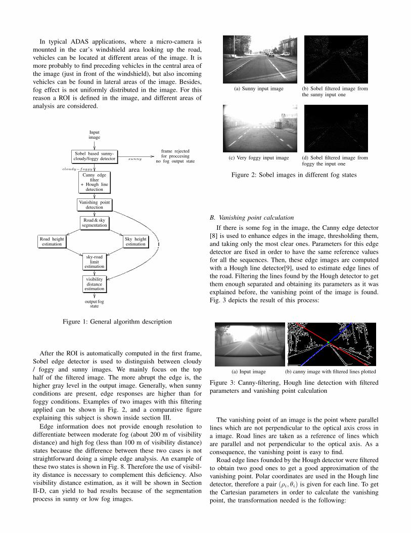
This section provides general information about the pro-posed algorithm. First of all, a general block diagram of theimplemented algorithm is shown in Fig. 1. Then the mostimportant blocks will be described.

A. Sobel based sunny - foggy detector

One of the most important effects of fog presence on aimage is the reduction of high frequency components, that canbe properly measured using edge detection methods, based onSobel filtering [7]. Foggy images are blurrier and have lowercontrast than the sunny ones. It means that information in thehigher frequencies is lower in foggy images, rather than insunny ones. Furthermore, this effect is more significant in thetop half of the image.

In order to reduce processing time in the whole algorithm,the original B&W images captured from the micro-camera areresized to 320 x 240 pixels. It is not necessary to have a higherresolution for fog detection.

In typical ADAS applications, where a micro-camera ismounted in the car’s windshield area looking up the road,vehicles can be located at different areas of the image. It ismore probably to find preceding vehicles in the central area ofthe image (just in front of the windshield), but also incomingvehicles can be found in lateral areas of the image. Besides,fog effect is not uniformly distributed in the image. For thisreason a ROI is defined in the image, and different areas ofanalysis are considered.

Inputimage

��Sobel based sunny-

cloudy/foggy detector sunny//

cloudy−foggy ��

frame rejectedfor proccesing

no fog output state

Canny edgefilter

+ Hough linedetection

��Vanishing point

detection

��

tt

Road & skysegmentation

((QQQQQvvmmmmm

Road heightestimation

''PPPPPPSky heightestimation

wwoooooo

sky-roadlimit

estimation

��visibilitydistance

estimation

��output fog

state

Figure 1: General algorithm description

After the ROI is automatically computed in the first frame,Sobel edge detector is used to distinguish between cloudy/ foggy and sunny images. We mainly focus on the tophalf of the filtered image. The more abrupt the edge is, thehigher gray level in the output image. Generally, when sunnyconditions are present, edge responses are higher than forfoggy conditions. Examples of two images with this filteringapplied can be shown in Fig. 2, and a comparative figureexplaining this subject is shown inside section III.

Edge information does not provide enough resolution todifferentiate between moderate fog (about 200 m of visibilitydistance) and high fog (less than 100 m of visibility distance)states because the difference between these two cases is notstraightforward doing a simple edge analysis. An example ofthese two states is shown in Fig. 8. Therefore the use of visibil-ity distance is necessary to complement this deficiency. Alsovisibility distance estimation, as it will be shown in SectionII-D, can yield to bad results because of the segmentationprocess in sunny or low fog images.

(a) Sunny input image (b) Sobel filtered image fromthe sunny input one

(c) Very foggy input image (d) Sobel filtered image fromfoggy the input one

Figure 2: Sobel images in different fog states

B. Vanishing point calculation

If there is some fog in the image, the Canny edge detector[8] is used to enhance edges in the image, thresholding them,and taking only the most clear ones. Parameters for this edgedetector are fixed in order to have the same reference valuesfor all the sequences. Then, these edge images are computedwith a Hough line detector[9], used to estimate edge lines ofthe road. Filtering the lines found by the Hough detector to getthem enough separated and obtaining its parameters as it wasexplained before, the vanishing point of the image is found.Fig. 3 depicts the result of this process:

(a) Input image (b) canny image with filtered lines plotted

Figure 3: Canny-filtering, Hough line detection with filteredparameters and vanishing point calculation

The vanishing point of an image is the point where parallellines which are not perpendicular to the optical axis cross ina image. Road lines are taken as a reference of lines whichare parallel and not perpendicular to the optical axis. As aconsequence, the vanishing point is easy to find.

Road edge lines founded by the Hough detector were filteredto obtain two good ones to get a good approximation of thevanishing point. Polar coordinates are used in the Hough linedetector, therefore a pair (ρi, θi) is given for each line. To getthe Cartesian parameters in order to calculate the vanishingpoint, the transformation needed is the following:

ai = cos (θi) , bi = sin (θi) =⇒ αi = −ai

bi, βi =

ρ

bi(1)

On the image, these two filtered lines would have thefollowing equations:

v0 = α1u0 + β1 (2)

v0 = α2u0 + β2 (3)

where (α1, β1) and (α2, β2) are the two lines parametersin Cartesian coordinates, converted from polar coordinates,which are obtained from the Hough transform. Solving theselast two equations the following one will be obtained:

u0 =β2 − β1

α1 − α2(4)

and substituting u0 in one of the two line equations above,the vanishing point height v0 can be found. An example ofthis procedure can be seen in Fig. 3.

C. Road and sky segmentation

After the vanishing point is found, a segmentation processis applied using a growing regions approach based on seeds,described in [10], to find the limit between the sky and theroad.

Sky is easy to find if it is present because pure white coloris present in the most part of sky pixels, and segmentationprocess is fast. A single seed point is selected and it is thefirst pure-white pixel on the supposed sky area.

For obtaining the road segmentation, the seed point is fixed,placing it in an area which is highly probable to find theroad, and some parameters have to be tuned, depending onroad’s characteristics, specifically in the average value of graylevel in a neighborhood of a road pixel. Depending on thisaverage level, the upper difference limit goes up when roadgets brighter. This is because the brighter the road is, thegreater variation of gray level the pixels in a neighborhood isobtained. Some road image samples from the tested sequencesare depicted in Fig. 4 to show the different conditions that thegrowing regions algorithm has to deal with.

(a) cloudy and low fogroad image

(b) cloudy and high fogroad image

(c) sunny road image(with shadows)

Figure 4: Image samples to show the different characteristicsof the road

To make the process of finding the sky-road limits easierto the rest of the algorithm, a dilation is applied to the skyimage. The growing regions algorithm leave some holes whichnot belongs to the segmented region inside it. The color usedto apply the segmentation process is white, so a dilation is

used to fill these holes in. In road segmentation the used coloris black, because there are not pure black color in a normalimage and, if it were white, it would be confused with sky andwrong results would be obtained. In this case, an erosion isused instead of dilation, because of the color used to determinethe road region.

In order to find the limit between the sky and the road,these two segmented images are treated separately. Sky androad image limits are searched from bottom to top, but thereare some differences in the procedure. Taking the average ofthis two limits, the limit between sky and road is found. Ifthe sky is not present, like in some of the test sequences, onlythe road limit is taken. In the case of the sky image, the mostcommon effect is that the part of the sky over the ground isnarrow and the part in the sky is wider. In this case, there is anabrupt transition that can be easily located. On the other hand,considering the road segmented image this abrupt transition isnot significant. If the road is well segmented, it is limitedby the gray zone in which it is located, but if the scene isvery foggy a bad segmentation or an erroneous limit can beobtained. In both cases, if the obtained limit is not logical, i.e.it is above the vanishing point, the vanishing point height willbe used as the limit for that frame.

In Fig. 5, some examples of segmented images using theproposed method are shown for the sky 5.b and the road 5.c.When the input image is foggy, a part of the road is segmentedin the sky image when this algorithm is used. On the one hand,in the sky image, the white part of the image which is thenarrowest, is considered the sky limit. On the other hand, inthe road image, when no black color is detected, the limit isestablished.

(a) sky segmented image (b) road segmented image

Figure 5: Segmented foggy images to find road and sky limits

D. Visibility distance measurement

Visibility distance depends on the relative sky-height. Thisconcept means that, when there is some fog in a scene androad is segmented, some part of sky gets into the road part,and the limit between the sky and the road go down. If theimage is not foggy, sky and road height on the image are boththe same and equals to the vanishing point height, but in afoggy image, apparent sky height is lower than the vanishingpoint.

This algorithm works with a monocular camera, therefore3D structure information is not directly available, but anestimation can be made using camera projection equationsprojection. In general,

u =X −X0

Z + f(5)

v =Y − Y0

Z + f(6)

The infinite depth distance (z →∞) is projected into thevanishing point (u0, v0) according to:

u0 = limz→∞

X −X0

Z + f= 0 (7)

v0 = limz→∞

Y − Y0

Z + f= 0 (8)

However, the solution (0, 0) is not a normal point ofprojection, so the Eq. 5 and 6 have to be rewritten as follows:

u− u0 =X −X0

Z + f(9)

v − v0 =Y − Y0

Z + f(10)

The “Y” axis is selected because fog effect affects theapparent height of the sky on the image, as can be seen inFig. 5, and X is independent from this effect. By using Eq.10 Z component can be solved. If a good camera calibrationis known, a good depth estimate can be obtained according tothe following:

Z = fY − Y0

v − v0+ f (11)

where Y − Y0 and f can be easily obtained from thecalibration process, since is the relative height from the groundto the camera and the focus distance respectively; v is beobtained from the relative sky height on the image and v0from the height of the vanishing point.

To obtain the depth ’Z’ component, we obtain the differencebetween the vertical coordinate of the limit sky – road, andthe vanishing point as it was explained before. With thisdifference computed and the calibration parameters of thecamera, we project this into the 3D world and obtain thedepth distance. Calibration parameters were experimentallyestimated to obtain reasonable values of visibility distance onthe tested sequences.

The estimation in a single frame is very unstable becausethe limit between sky-road can variate substantially dependingon the segmentation results and the camera saturation. Inaddition, the vanishing point height can also variate due tocar vibrations.

Because of that, a filter to alleviate these effects has beenimplemented. The adopted solution for this problem is totake the median every T seconds. In this period of time, thevanishing point heights and sky-road, limits are registered andthe median of each array is calculated when every period isfinished. This time is long enough to ease the effects of car’s

vibrations and fluctuations in the estimated sky-road limit.Another trials have been made, e.g. taking the average insteadof the median, or registering samples during a shorter periodof time.

Once these two parameters are obtained and Z componentis calculated, the specified limits in Table I are used in orderto differentiate between the different fog levels. The maximumtheoretical visibility distance is about 2 km or above and thereis no minimum for visibility distance as it depends on thesky road limit and the calibration parameters. These are basedon a common meteorologic criteria to establish the visibilitydistance.

upper limit (m) lower limit (m)low fog - sunny - 300

moderate fog 300 100high fog 100 -

Table I: Visibility distance limits for each fog state

III. RESULTS

In this section the results of the algorithm are shown. Firstly,we show Sobel edge detector results, then some results withoutand with Sobel edge information will be shown to prove thenecessity of the both systems working together, and finallysome global statistics about confidence rates of the wholealgorithm are described.

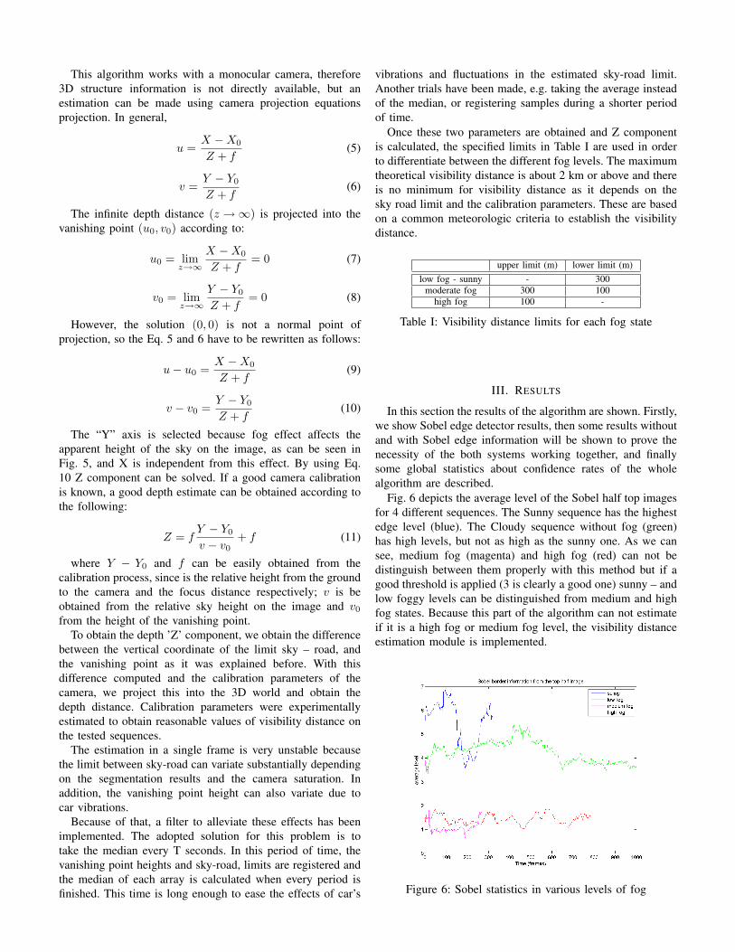
Fig. 6 depicts the average level of the Sobel half top imagesfor 4 different sequences. The Sunny sequence has the highestedge level (blue). The Cloudy sequence without fog (green)has high levels, but not as high as the sunny one. As we cansee, medium fog (magenta) and high fog (red) can not bedistinguish between them properly with this method but if agood threshold is applied (3 is clearly a good one) sunny – andlow foggy levels can be distinguished from medium and highfog states. Because this part of the algorithm can not estimateif it is a high fog or medium fog level, the visibility distanceestimation module is implemented.

Figure 6: Sobel statistics in various levels of fog

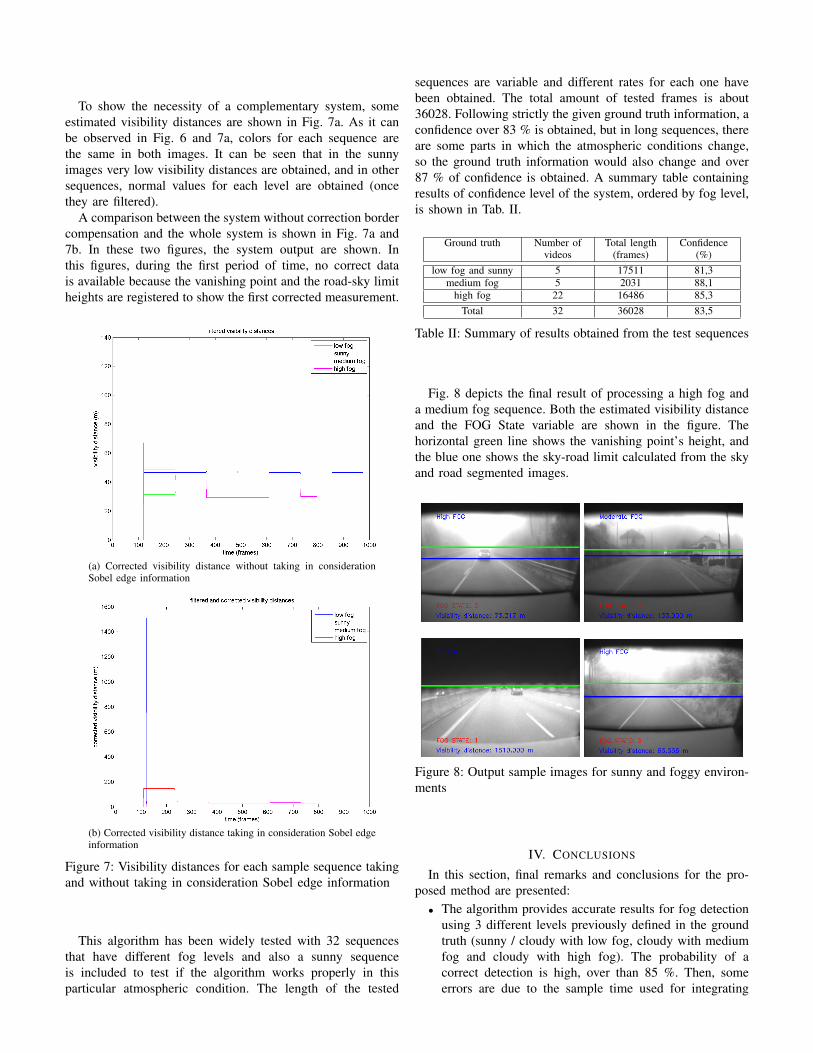
To show the necessity of a complementary system, someestimated visibility distances are shown in Fig. 7a. As it canbe observed in Fig. 6 and 7a, colors for each sequence arethe same in both images. It can be seen that in the sunnyimages very low visibility distances are obtained, and in othersequences, normal values for each level are obtained (oncethey are filtered).

A comparison between the system without correction bordercompensation and the whole system is shown in Fig. 7a and7b. In these two figures, the system output are shown. Inthis figures, during the first period of time, no correct datais available because the vanishing point and the road-sky limitheights are registered to show the first corrected measurement.

(a) Corrected visibility distance without taking in considerationSobel edge information

(b) Corrected visibility distance taking in consideration Sobel edgeinformation

Figure 7: Visibility distances for each sample sequence takingand without taking in consideration Sobel edge information

This algorithm has been widely tested with 32 sequencesthat have different fog levels and also a sunny sequenceis included to test if the algorithm works properly in thisparticular atmospheric condition. The length of the tested

sequences are variable and different rates for each one havebeen obtained. The total amount of tested frames is about36028. Following strictly the given ground truth information, aconfidence over 83 % is obtained, but in long sequences, thereare some parts in which the atmospheric conditions change,so the ground truth information would also change and over87 % of confidence is obtained. A summary table containingresults of confidence level of the system, ordered by fog level,is shown in Tab. II.

Ground truth Number ofvideos

Total length(frames)

Confidence(%)

low fog and sunny 5 17511 81,3medium fog 5 2031 88,1

high fog 22 16486 85,3Total 32 36028 83,5

Table II: Summary of results obtained from the test sequences

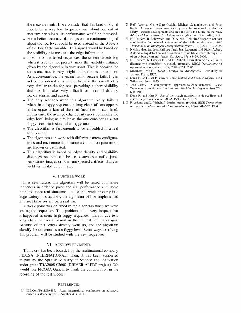
Fig. 8 depicts the final result of processing a high fog anda medium fog sequence. Both the estimated visibility distanceand the FOG State variable are shown in the figure. Thehorizontal green line shows the vanishing point’s height, andthe blue one shows the sky-road limit calculated from the skyand road segmented images.

Figure 8: Output sample images for sunny and foggy environ-ments

IV. CONCLUSIONS

In this section, final remarks and conclusions for the pro-posed method are presented:• The algorithm provides accurate results for fog detection

using 3 different levels previously defined in the groundtruth (sunny / cloudy with low fog, cloudy with mediumfog and cloudy with high fog). The probability of acorrect detection is high, over than 85 %. Then, someerrors are due to the sample time used for integrating

the measurements. If we consider that this kind of signalshould be a very low frequency one, about one outputmeasure per minute, its performance would be increased.

• For a better accuracy of the system, a continuous signalabout the fog level could be used instead of the 3 levelsof the Fog State variable. This signal would be based onthe visibility distance and the edge information.

• In some of the tested sequences, the system detects fogwhen it is really not present, since the visibility distancegiven by the algorithm is very short. This is because thesun sometimes is very bright and saturates the camera.As a consequence, the segmentation process fails. It cannot be considered as a failure, because the sun effect isvery similar to the fog one, provoking a short visibilitydistance that makes very difficult for a normal driving,i.e. on sunrise and sunset.

• The only scenario when this algorithm really fails iswhen, in a foggy sequence, a long chain of cars appearsin the opposite lane of the road (near the horizon line).In this case, the average edge density goes up making theedge level being as similar as the one considering a notfoggy scenario instead of a foggy one.

• The algorithm is fast enough to be embedded in a realtime system.

• The algorithm can work with different camera configura-tions and environments, if camera calibration parametersare known or estimated.

• This algorithm is based on edges density and visibilitydistances, so there can be cases such as a traffic jams,very sunny images or other unexpected artifacts, that canyield an invalid output value.

V. FURTHER WORK

In a near future, this algorithm will be tested with moresequences in order to prove the real performance with moretime and more real situations, and once it work properly in ahuge variety of situations, the algorithm will be implementedin a real time system on a real car.

A weak point was obtained in the algorithm when we weretesting the sequences. This problem is not very frequent butit happened in some high foggy sequences. This is due to along chain of cars appeared in the top half of the images.Because of that, edges density went up, and the algorithmclassify the sequence as not foggy level. Some ways to solvingthis problem will be studied with the new sequences.

VI. ACKNOWLEDGMENTS

This work has been bounded by the multinational companyFICOSA INTERNATIONAL. Then, it has been supportedin part by the Spanish Ministry of Science and Innovationunder grant TRA2008-03600 (DRIVER-ALERT project). Wewould like FICOSA-Galicia to thank the collaboration in therecording of the test videos.

REFERENCES

[1] IEE.Conf.Publ.No.483. Adas. international conference on advanceddriver assistance systems. Number 483, 2001.

[2] Rolf Adomat, Georg-Otto Geduld, Michael Schamberger, and PeterReith. Advanced driver assistance systems for increased comfort ansafety - current developments and an outlook to the future on the road.Advanced Microsystems for Automotive Applications, 2:431–446, 2003.

[3] N. Hautière, R. Labayrade, and D. Aubert. Real-time disparity contrastcombination for onboard estimation of the visibility distance. IEEETransactions on Intelligent Transportation Systems, 7(2):201–212, 2006.

[4] Nicolas Hautière, Jean-Philippe Tarel, Jean Lavenant, and Didier Aubert.Automatic fog detection and estimation of visibility distance through useof an onboard camera. Mach. Vis. Appl., 17(1):8–20, 2006.

[5] N. Hautière, R. Labayrade, and D. Aubert. Estimation of the visibilitydistance by stereovision: A generic approach. IEICE Transactions oninformation and systems, 89(7):2084–2091, 2006.

[6] Middleton W.E.K. Vision Through the Atmosphere. University ofToronto Press, 1952.

[7] Duda R. and Hart P. Pattern Classification and Scene Analysis. JohnWiley and Sons, 1973.

[8] John Canny. A computational approach to edge detection. IEEETransactions on Pattern Analysis and Machine Intelligence, 8(6):679–698, 1986.

[9] Duda R. and Hart P. Use of the hough transform to detect lines andcurves in pictures. Comm. ACM, 15(1):11–15, 1972.

[10] R. Adams and L. Vishchof. Seeded region growing. IEEE Transactionson Pattern Analysis and Machine Intelligence, 16(6):641–657, 1994.