fMRI Methods Lecture3 – Modeling the neurovascular coupling
52
fMRI Methods Lecture3 – Modeling the neurovascular coupling
-
Upload
dale-scott -
Category
Documents
-
view
45 -
download
1
description
fMRI Methods Lecture3 – Modeling the neurovascular coupling. Hemodynamic changes. Neurons. Synaptic transmission. Majority of the synapses in the cortex are excitatory glutamate synapses. Synaptic transmission. Neurotransmitter vesicles. - PowerPoint PPT Presentation
Transcript of fMRI Methods Lecture3 – Modeling the neurovascular coupling

fMRI Methods
Lecture3 – Modeling the neurovascular coupling
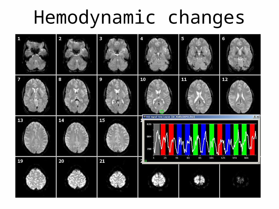
Hemodynamic changes

Neurons
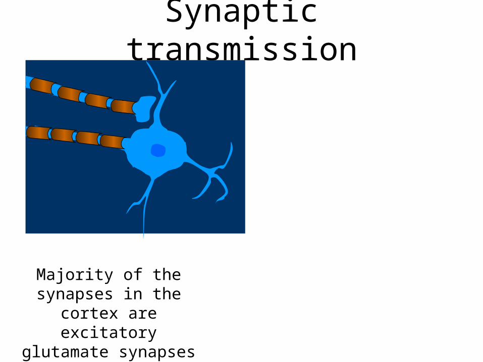
Synaptic transmission
Majority of the synapses in the cortex are excitatory
glutamate synapses

Synaptic transmission
Neurotransmitter vesicles
Majority of the synapses in the cortex are excitatory
glutamate synapses

Synaptic transmission
Neurotransmitter releases into the synaptic cleft and
binds to receptors
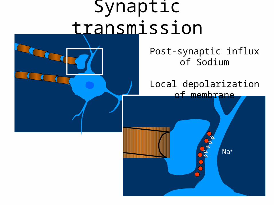
Synaptic transmission
Post-synaptic influx of Sodium
Local depolarization of membrane
Na+
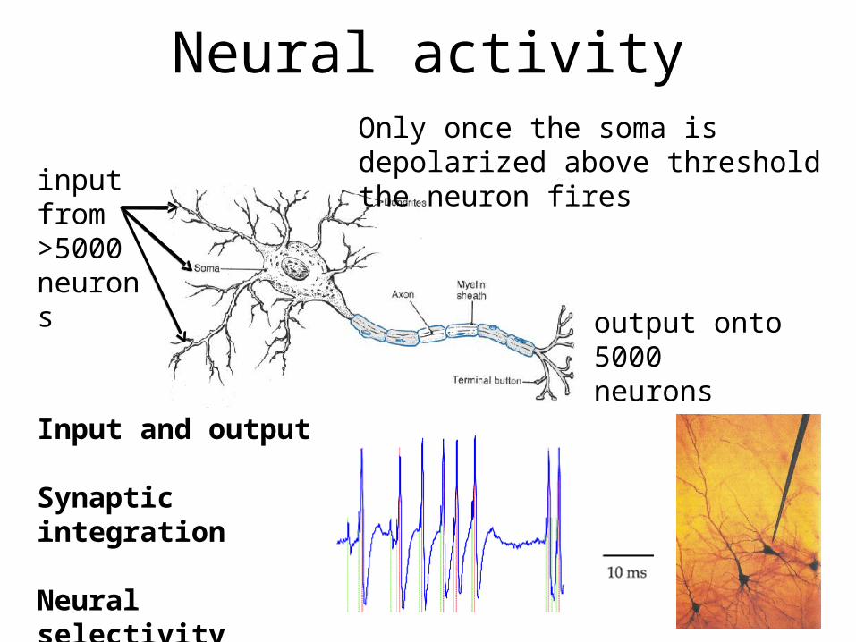
Neural activity
inputfrom >5000 neurons
Only once the soma is depolarized above threshold the neuron fires
Input and output
Synaptic integration
Neural selectivity
output onto 5000 neurons

Cortical architectureLot’s of local reciprocal connections in the cortex. 80% of synapses are onto neighboring neurons within 1mm.
What’s the input and what’s the output?Lot’s of correlated activity among neighbors (columns)

Resolution
With an electrode we can isolate the activity of a few neighboring neurons.
Do single neurons represent what’s happening in the network?
You can describe brain activity at different levels of resolution.
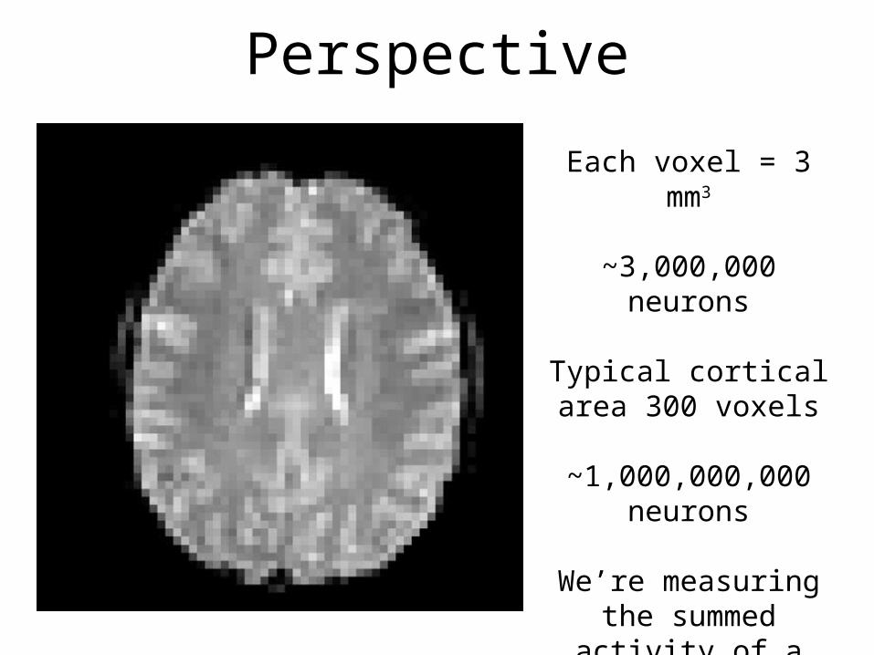
Perspective
Each voxel = 3 mm3
~3,000,000 neurons
Typical cortical area 300 voxels
~1,000,000,000neurons
We’re measuring the summed activity of a huge neural network.

Neurovascular coupling
Relationship between neural activity and hemodynamics

Birth of the HRF
How do we characterize the hemodynamic response associated with a particular neural
response?
We look at primary visual cortex

Birth of the HRF
Boynton et. al. 1996

Birth of the HRF
The HRFs above have a characteristic shape that can be approximated by a gamma function.
Boynton et. al. 1996
This function has two free parameters:Tau - time to peak n - time shift (amount of delay)
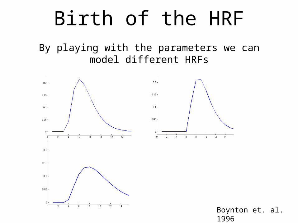
Birth of the HRFBy playing with the parameters we can model
different HRFs
Boynton et. al. 1996

Birth of the HRF
So we can either measure our subject’s specific HRF or use a “canonical” HRF from the literature
We assume that the same relationship found in primary visual cortex applies everywhere.
Might be reasonable for the cortex where the neural architecture is more or less the same.
Subcortical areas?

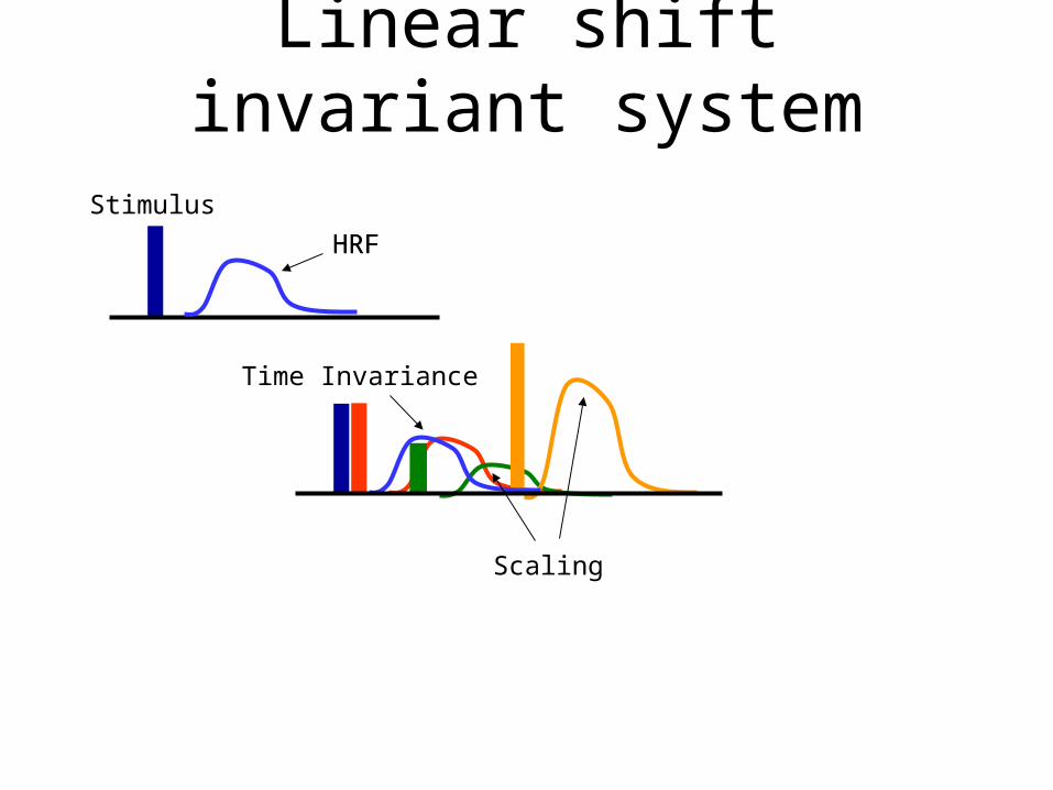
Stimulus
HRFHRF
Time Invariance
Linear shift invariant system
Very simple coupling between neural activity and hemodynamics
Linear shift invariant system
Stimulus
HRFHRF
Scaling
Time Invariance
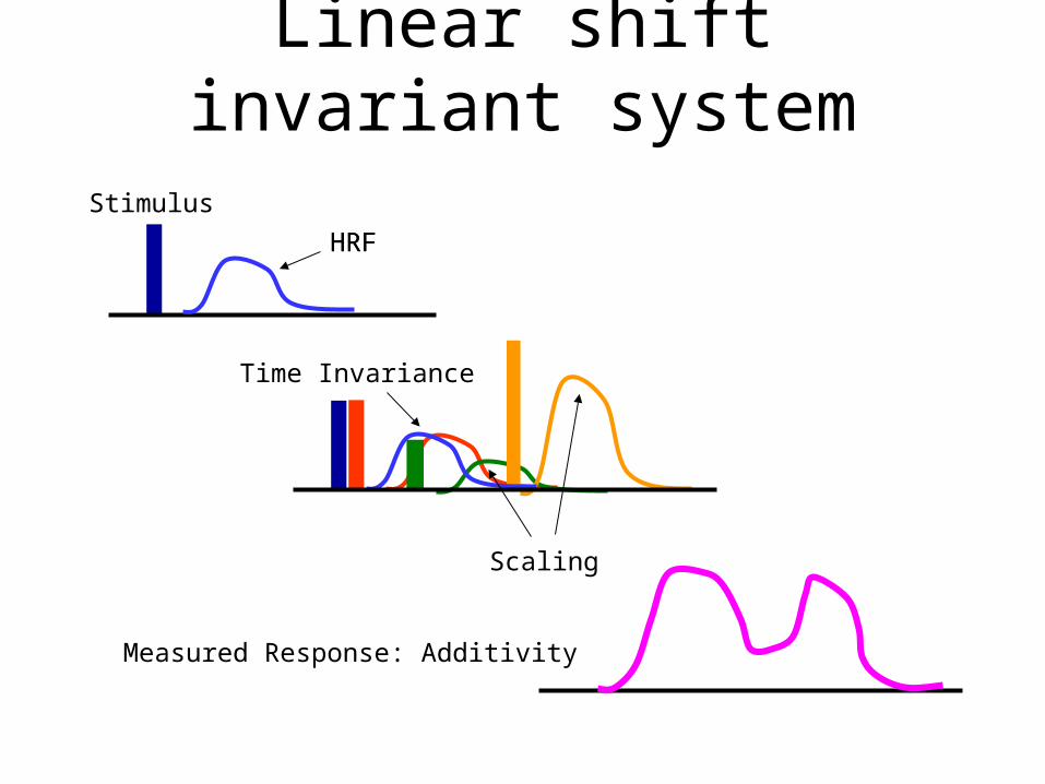
Linear shift invariant system
Stimulus
HRFHRF
Scaling
Time Invariance
Measured Response: Additivity

Linear shift invariant system
The linear transformation step is simply a convolution with a hemodynamic impulse
response function

Convolution
Multiply each timepoint of the neural response by a copy of the HRF

Temporal summationWhen convolving with an HRF we are actually
“smoothing” our data.
We loose temporal resolution because we create a lot of correlation between neighboring timepoints.
Original audio: Smoothed audio:
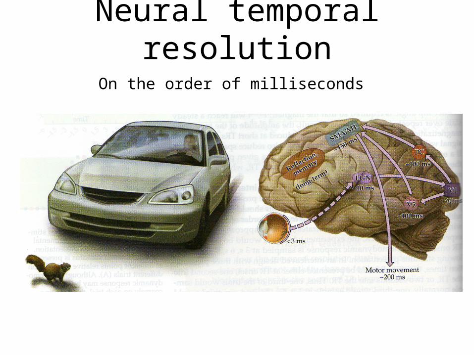
Neural temporal resolution
On the order of milliseconds
The challenges
Spatial: we’re sampling the average activity of millions of neurons distributed across space.
Temporally: we’re sampling the average activity of these neurons across several seconds in time.
But, we don’t need to cut anybody’s head open…

Estimating neural activity
So far we’ve been estimating hemodynamic responses from neural activity.
We actually want to go the other way around.

Experimental design
Because of the sluggishness of the hemodynamic responses we want to build slow experiments.
Need to consider our signal to noise:How clean are our measurements?Should we repeat them many times and average?
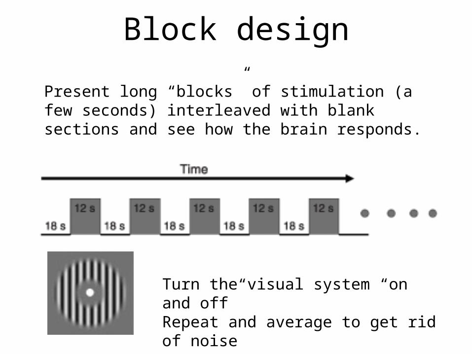
Block design
Present long “blocks” of stimulation (a few seconds) interleaved with blank sections and see how the brain responds.
Turn the visual system “on and off”Repeat and average to get rid of noise

Block designWe assume that the stimulus is generating prolonged sustained neural activity for the entire length of stimulus presentation and with equal amplitude on consecutive blocks.
Model of expected neural activity
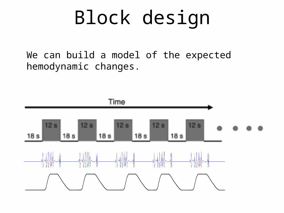
Block design
We can build a model of the expected hemodynamic changes.

CorrelationHow can we relate the model with the actual data we
measured in the scanner?
One option is to correlate…
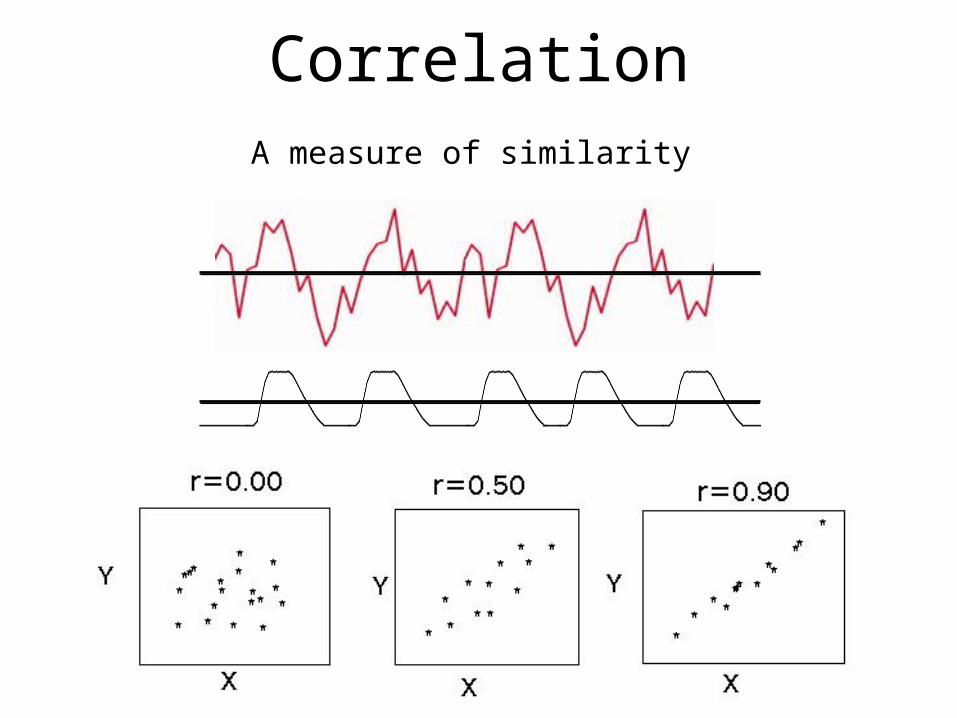
CorrelationA measure of similarity
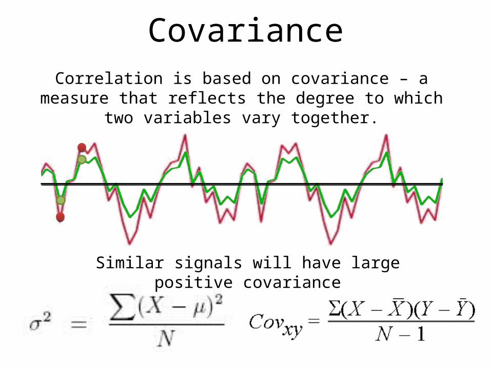
CovarianceCorrelation is based on covariance – a measure that
reflects the degree to which two variables vary together.
Similar signals will have large positive covariance

CovarianceCorrelation is based on covariance – a measure that
reflects the degree to which two variables vary together.
Opposite signals will have large negative covariance
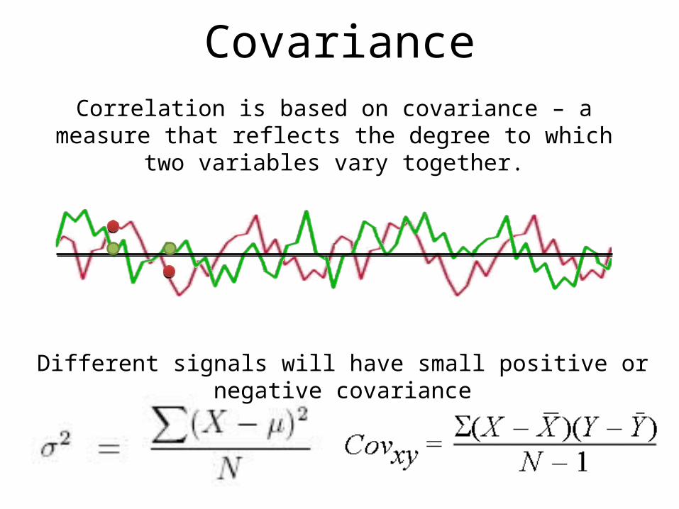
CovarianceCorrelation is based on covariance – a measure that
reflects the degree to which two variables vary together.
Different signals will have small positive or negative covariance

CorrelationCorrelation is the covariance divided (normalized) by the
variance of the two signals
This last bit ensures that correlation coefficients have values between -1 and 1.
It also means that the scaling/amplitude/variance of the signal doesn’t matter when computing correlation!
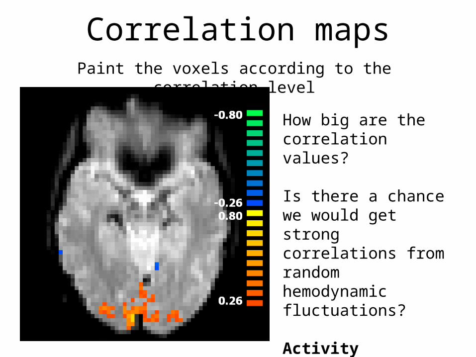
Correlation mapsPaint the voxels according to the correlation level
How big are the correlation values?
Is there a chance we would get strong correlations from random hemodynamic fluctuations?
Activity localization

Estimating response amplitudeBut we also want to estimate response strength
How much do we need to scale the model so that it best fits the data?

General linear modelExplain the recorded data with a model composed from a combination of linear predictors.
data = a0 + a1x1 + a2x2 + … + a3x3 + error
data: voxel time-coursea: parameter weights (often called beta weights)x: model factor/predictore: error (what’s left over in the data that is not explained by the model)

General linear modelIn our example so far we had a model with only one predictor.
data = a0 + a1x1 + error
Our predictor described the hemodynamic activity expected based on our experiment structure.
x1 =

General linear modelWe can describe the previous equation as:
= * + errora1
We want to find a1 that will minimize the error term (best fit).
data
design matrix beta
residuals

RegressionIn our example the beta weight minimizing the error term will equal the slope of the regression line when regressing the predictor (x) onto the data (y):
y’ = a*x + c
regression line
slope intercept
predictor
What happened to the ‘error’ (residuals)?

RegressionThe slope (a) is the covariance divided/normalized only by the variance of the predictor. This makes the slope dependant on the variance in the data (y)…
Correlation:
Regression
y’ = a*x + c
regression line
slope intercept
predictor

Least squares optimization
Find the beta weight (a) that will minimize the squared error:
datadesign matrix
In our example the solution is to find the projection of the single predictor onto the data (it’s their dot product).
Open least squares handout.

Multiple predictors
In most experiments we have more than one predictor.We’ll have different experimental conditions and we’ll want to compare the responses to each.

Multiple predictorsWe will have a separate column for each predictor in our design matrix and a separate associated beta weight.
= * + errora1 a2
data
design matrix
beta
residuals
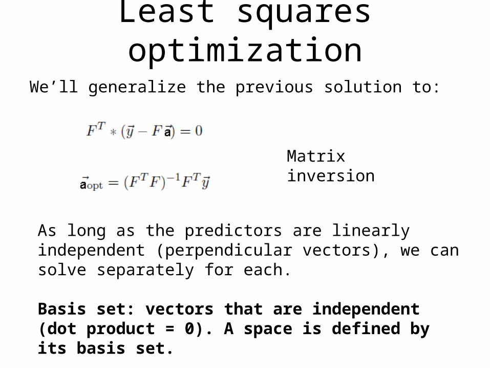
Least squares optimization
We’ll generalize the previous solution to:
As long as the predictors are linearly independent (perpendicular vectors), we can solve separately for each.
Basis set: vectors that are independent (dot product = 0). A space is defined by its basis set.
Matrix inversion

Beta value mapsPaint the voxels by their beta value (response amplitude):
Does not take model fit (noise) into account.

Statistical parameter mapsPaint the voxels by the statistical significance of the betas:
p values from a t-test.
Takes model fit (noise) into account.

Break
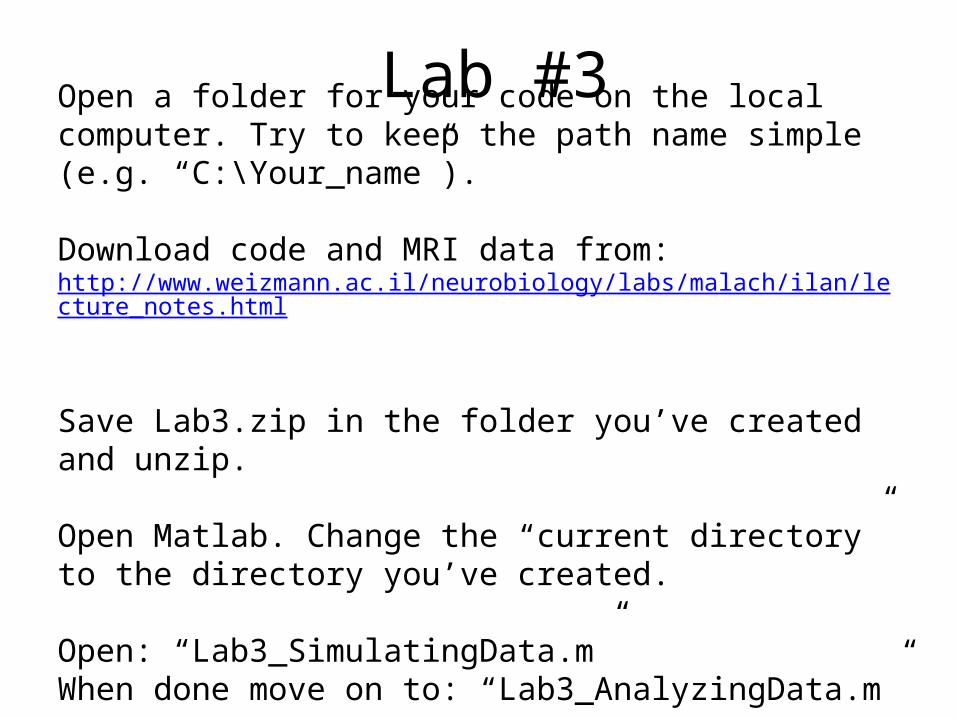
Open a folder for your code on the local computer. Try to keep the path name simple (e.g. “C:\Your_name”).
Download code and MRI data from:http://www.weizmann.ac.il/neurobiology/labs/malach/ilan/lecture_notes.html
Save Lab3.zip in the folder you’ve created and unzip.
Open Matlab. Change the “current directory” to the directory you’ve created.
Open: “Lab3_SimulatingData.m”When done move on to: “Lab3_AnalyzingData.m”
Lab #3

Read Chapters 6-8 of Huettel et. al.
Go over least squares handout
Matlab exercise: email me the report as a word document. The report should include answers, figures, and the actual Matlab code used to generate them (copy it into word).
Homework!