Fluid–structure simulation of a viscoelastic hydrofoil ...

Fluid–structure simulation of a viscoelastichydrofoil subjected to quasi-steady flow

R. L. Campbell, E. G. Paterson, M. C. Reese & S. A. HambricPenn State Applied Research Laboratory, USA

Abstract

Fluid–structure interaction simulations are performed for a flexible hydrofoilsubjected to quasi-steady flow conditions. The hydrofoil is fabricated from apolymeric material that exhibits viscoelastic effects, causing the hydrofoil tochange shape while subjected to the fluid loads. The time-dependent deformationsand loads will be compared in the future to empirical results from upcoming watertunnel tests. The fluid–structure interaction simulations are performed using atightly coupled partitioned approach, with OpenFOAM as the flow solver and afinite element solver for the structural response. The codes are coupled using afixed-point iteration with relaxation. The flow is modeled as laminar and quasi-steady. Simulations indicate the hydrofoil angle of attack (AOA) changes fromzero to a negative value as the material relaxes. The approach used here is beingdeveloped for application to a blood pump that has a performance closely tied toblade deformation through the impeller tip clearance.Keywords: fluid–structure interaction, viscoelasticity, hydrofoil, OpenFOAM.

1 Introduction

The area of fluid–structure interaction (FSI) modeling has been very active inrecent years, as evidenced by the numerous papers in the literature (see, forexample, the review by Tezduyar and Sathe [1]). The dramatic advances inaffordable computational resources coupled with improved modeling capabilityfor both fluid and solid structures over the past two decades have made feasiblecoupled fluid/solid simulations for real-world engineering applications. WhileFSI simulations have been an area of research since the late 1970s (see Felippaet al. [2]), there still exist several challenges before these simulations will be

Advances in Fluid Mechanics VIII 439

www.witpress.com, ISSN 1743-3533 (on-line) WIT Transactions on Engineering Sciences, Vol 69, © 2010 WIT Press

doi:10.2495/AFM100381

routinely applied to real-world engineering applications (Tezduyar and Sathe [1]and Longatte et al. [3]).

The present application is related to a flexible blood pump impeller with a tipclearance (i.e., the clearance between the blade tips and the pump housing) that isvery sensitive to blade deflections. The impeller is fabricated from a polymer thathas a time-dependent response to applied loads (creep) and enforced displacements(stress relaxation), and therefore requires the use of a viscoelastic material model.The influence of blade deformation on pump performance is expected to be verystrong because of the anticipated tip gap changes.

The approach to solving this problem involves several steps. The first step isto implement a FSI solver capable of modeling the nonlinear, time dependentpolymeric material behaviour. Verification and validation of this solver is thesecond step and will be performed using a simple hydrofoil constructed of thesame polymer as the blood pump impeller, and subjected to flow in a water tunnelfor which net blade loads and blade deformation will be measured. The modelingapproach will then be modified and updated as necessary and then applied tothe actual rotating impeller of the blood pump. Time-dependent performancepredictions of the pump will be compared to empirical results. The focus of thecurrent paper is the fluid–structure simulations of the simple polymeric hydrofoiloperating in the water tunnel test section.

2 Problem description

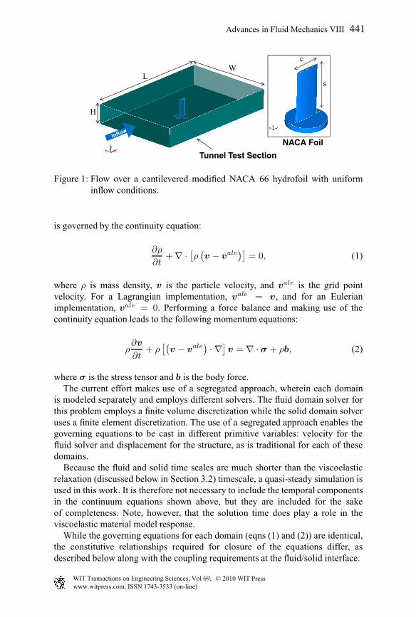
A single hydrofoil constructed of a polymeric material is affixed in a water tunneltest section with zero angle of attack (AOA). The hydrofoil is a modified NACAseries 66 with a = 0.8 camber [4] and thus has nonzero lift at zero AOA. Theupstream flow boundary is modeled as a uniform inflow with a velocity of 2 m/sand the downstream flow boundary is modeled with a zero pressure condition. Theno-slip condition is applied at all other fluid boundaries. The foil is constrainedat the root and is subjected to fluid pressures at the fluid/solid interface, ΓF/S . Aschematic of the setup is shown in figure 1. The test section has a length (L) of0.762 m, width (W) of 0.508 m, and height (H) of 0.114 m. The distance from theinlet to the foil leading edge is 0.356 m. The foil has a chord length (c) of 0.050 mand a span (s) of 0.100 m.

The Reynolds number, based on hydrofoil chord, for this flow is approximately100,000 and the critical Reynolds number for transition to turbulence is on theorder of 200,000. Therefore, it is reasonable to employ a laminar flow model forthe first attempt at modeling this problem.

3 Fluid–structure simulation approach

The governing equations for continuum mechanics (both fluids and solids), cast inan arbitrary Lagrangian Eulerian (ALE) form, are as follows. Mass conservation

440 Advances in Fluid Mechanics VIII


NACA Foil

Tunnel Test Section

H

LW

c

s

Figure 1: Flow over a cantilevered modified NACA 66 hydrofoil with uniforminflow conditions.

is governed by the continuity equation:

∂ρ

∂t+ ∇ · [ρ (v − vale

)]= 0, (1)

where ρ is mass density, v is the particle velocity, and vale is the grid pointvelocity. For a Lagrangian implementation, vale = v, and for an Eulerianimplementation, vale = 0. Performing a force balance and making use of thecontinuity equation leads to the following momentum equations:

ρ∂v

∂t+ ρ

[(v − vale

) · ∇]v = ∇ · σ + ρb, (2)

where σ is the stress tensor and b is the body force.The current effort makes use of a segregated approach, wherein each domain

is modeled separately and employs different solvers. The fluid domain solver forthis problem employs a finite volume discretization while the solid domain solveruses a finite element discretization. The use of a segregated approach enables thegoverning equations to be cast in different primitive variables: velocity for thefluid solver and displacement for the structure, as is traditional for each of thesedomains.

Because the fluid and solid time scales are much shorter than the viscoelasticrelaxation (discussed below in Section 3.2) timescale, a quasi-steady simulation isused in this work. It is therefore not necessary to include the temporal componentsin the continuum equations shown above, but they are included for the sakeof completeness. Note, however, that the solution time does play a role in theviscoelastic material model response.

While the governing equations for each domain (eqns (1) and (2)) are identical,the constitutive relationships required for closure of the equations differ, asdescribed below along with the coupling requirements at the fluid/solid interface.



3.1 Flow solver

OpenFOAM is the flow solver of choice for this effort because it facilitatescustom integration with third-party solvers, has a pre-existing, robust mesh motioncapability, and it is freely available through the GNU General Public License. Theautomatic mesh motion solver for the current problem makes use of a variablediffusion coefficient with quadratic dependence on the distance from the movingboundary (i.e., γ = 1/l2), see Jasak and Tukovic [5]. The flow for this problemis approximated as incompressible and laminar, and the stress-strain closure ismodeled as Newtonian:

σ = −pI + 2µS, (3)

where p is the thermodynamic pressure, µ is the absolute viscosity, I is the secondrank unity tensor, and S is the strain-rate tensor.

3.2 Structural solver and solid model

The structural solver employed for this work uses a Lagrangian finite element(FE) implementation, which means the mesh velocity is equivalent to the materialvelocity, vale = v. The momentum equation (eqn 2) becomes:

ρ∂2u

∂t2= ∇ · σ + ρb, (4)

where u are the material displacements.One of the important aspects of the current problem is the time dependency of

the polymeric material. The time dependency is a result of a viscous-like materialbehaviour. The material also exhibits elasticity in that it will not continue toflow unbounded with the application of a finite stress. The viscoelasticity modelemployed for this work follows an approach similar to that used by the commercialsoftware Abaqus (see the Abaqus User’s Manual [6]) and derived in a similarmanner by Kaliske and Rothert [7]. This model is for linear viscoelastic materials(which does not mean the time response of the material is linear, but rather thestress is proportional to strain at any given time: ε [cσ(t)] = cε [σ(t)], where cis a constant) and uses the approximation that shear and volumetric behavior areindependent. Experimental evaluation of the current material suggests that onlythe shear terms need to be modified by the viscoelastic model, which is consistentwith most material behavior as reported by Kaliske and Rothert [7] and also in theAbaqus Manual [6].

The underlying material model is that of the Generalized Maxwell Element,which consists of Maxwell elements (i.e., a spring and dashpot in series) in parallelwith a Hooke element (i.e., a spring) as shown in figure 2. The spring stiffnessshown in this figure represents the material stiffness at infinite time (i.e., after allof the viscoelastic forces have diminished to zero). Each of the Maxwell elementsare represented by a term in a Prony series (a series of the form

∑Ni=1 γie

−t/τi)representation of the material, which is further described below.



µ0

µ1 µ2 µN

η1 η2 ηN

Figure 2: General Maxwell element with N components.

The stress is decomposed into hydrostatic and deviatoric components in orderto isolate the viscoelastic effect from the volumetric terms:

σn+1 = κ tr εn+1I + dev σn+1, (5)

where κ is the bulk modulus, tr εn+1 is the trace of εn+1, and dev σn+1 is thedeviatoric part of the material stress tensor for the current (n + 1) time step. Thedeviatoric part of the stress takes on the following form:

dev σn+1 = dev σn+10 +

N∑i=1

hn+1i , (6)

where σ0 is the elastic stress tensor and hi are the internal stress variables thatcome from the so called heredity integral:

hi(t) =∫ t

o

γie− t−s

τi∂σ0(s)∂s

ds. (7)

Splitting this integral into parts that are known (i.e., time period [0, tn]) andunknown (i.e., time period [tn, tn+1]), and using the approximation ∂σ0(t)

∂t ≈σn+1

0 −σn0

∆t , the internal stress variables at the next time step are approximated asfollows:

hn+1i ≈ e

−∆tτi hn

i + γi1 − e

−∆tτi

∆tτi

[dev σn+1

0 − dev σn0

], (8)

where γi are the normalized relaxation constants, τi are the relaxation times, and∆t = tn+1 − tn is the time step. Both γi and τi represent terms of a Prony seriesand are determined from empirical data as described below.

Important for nonlinear finite element analyses using an implicit formulationwith a Newton algorithm is the material stiffness tensor. The tensor is computedas follows for the viscoelastic material:

Cn+1 = κII + 2µ0

[1 +

N∑i=1

γi1 − e

−∆tτi

∆tτi

](I − 1

3II

), (9)

where I is the fourth rank unity tensor.



0.4

0.6

0.8

1

0.1 1 10 100 1000 10000

σ/σ

0

Time, s

Stress Relaxation, 5% Strain

Data

Fit

Figure 3: Stress relaxation data and the resulting Prony series curve fit.

Table 1: Prony series stress relaxation parameters.

Component, i γi τi

1 0.1484 4.130

2 0.2115 8.195x101

3 0.1993 1.610x103

Relaxation constants and times, γi and τi, are determined from empirical stressrelaxation data of tensile test samples. The polymeric material used in this workhas a 95 A Shore hardness and is from the Hapflex line of materials purchasedfrom Hapco, Inc., Massachusetts USA. The constants are determined by a least-squares fit to uni-axial tensile stress relaxation data shown in figure 3 along withthe resulting fit. The parameters used to create this fit are provided in table 1. Theremaining parameters required for the structural model are the long term modulus,E0, and Poisson’s ratio, ν. The material is assumed to be nearly incompressibleand thus ν = 0.49 is used in the simulations. The long term modulus has beenestimated from empirical data to be E0 = 30.4 MPa.

The finite-element solver used for this effort has been been implemented bythe authors in the form of a C/C++ program that can easily be combined andcompiled with OpenFOAM. The use of a separate finite-element solver instead ofthe existing structural finite volume solver in OpenFOAM is a matter of preference.

3.3 Coupling approach

The algorithm defining the solution procedure is provided in figure 4. As indicatedin this figure, a fixed-point iteration is performed with under-relaxation to ensurethe fluid pressures and solid displacements are tightly converged before moving onto the next time step.



The under-relaxation approach employs the Aitken ∆2 method [8] to define thedynamic relaxation coefficient. The coefficient is calculated as follows:

ωi = −ωi−1rT

i (ri+1 − ri)|ri+1 − ri|2 , (10)

where ri = uΓF/S ,i − uΓF/S ,i−1 and uΓF/S ,i are the computed fluid/structureinterface displacements for iteration i. The prediction of the displacements forthe current iteration is then uΓF/S,i = uΓF/S ,i−1 + ωi

(uΓF/S,i − uΓF/S,i−1

),

as indicated in the coupling algorithm of figure 4. The iteration stops when|ri|/√n < ε, where n is the length of ri and ε is the error tolerance.

Solve Fluid

Solve Solid

/F SpΓ

Converged? t=t+δt

Move Fluid Mesh

ui = ωiûi - (1-ωi)ui-1 t>tend STOP

START

Fixed-Point Iteration

No Yes

Yes

No

i++ûi

Figure 4: Implicit coupling scheme with under-relaxation.

4 Simulation results

The important variables to monitor for the current simulation are blade deflectionand net blade load because these will be measured during the upcoming watertunnel tests. Sample results for the blade deflection, shown by blade tip sections,are provided in figure 5. The net blade forces, from integrating the fluid pressuresover ΓF/S are shown in figure 6. This figure shows results for a baseline model andthe viscoelastic model. The baseline model uses a constant constitutive relationshipwherein the modulus represents the material response to an instantaneouslyapplied load.

The blade AOA at the tip section changes from zero at the start of the simulationto increasingly negative values, reaching −8.1◦ at t = 360 s. The blade lift(lift = −Fy) decreases to zero after about 50 s of operation, and then continuesto decrease with time as indicated in figure 6. This figure also shows the largedifference in force magnitude between the baseline and viscoelastic models and thestrong temporal dependence of the viscoelastic model. Note that the the first 360 sof operation are shown in this figure. Results have been computed for longer timesand indicate the system is nearly at a steady state condition after approximatelyone hour of operation.



0 10 20 30 40 50

0

5

1

Blade Tip Section Locations

Axial Coordinate, mm

t=360st=270s

t=180s

t=90s

t=0

baseline

Figure 5: Blade tip section deflections; curves show results from differentsimulation times; baseline model response shown by dotted curve.

-2

-1

0

1

2

0 100 200 300

Net

For

ce, N

Time, s

Net Blade Force

Fmag,Baseline

Fmag

Drag

Lift

Fz

aselineFiscoF

iscorag F=

iscoF

iscoyLift F= −

Figure 6: Net blade forces for baseline (using the instantaneous modulus) andviscoelastic models.

5 Summary and conclusions

Tightly coupled FSI simulations have been used for a single hydrofoil sub-jected to quasi-steady flow to model the effects of a viscoelastic hydrofoiloperating in a water tunnel test section. The fluid domain is discretized usingthe finite volume approach, and solved using OpenFOAM. The flow is mod-eled as incompressible, laminar, and steady. The moving mesh in the fluiddomain is accomplished through the tetrahedral decomposition approach withLaplace smoothing, as implemented in OpenFOAM. The solid domain is dis-cretized with finite elements and solved using an author-written solver thatis compiled with the OpenFOAM solver to facilitate data transfer necessaryfor the domain coupling. Simulation results for blade deformations and loadswith respect to time show the dramatic effect of employing the viscoelasticconstitutive relationship instead of an equivalent material modulus. The AOA



of the blade monotonically decreases from zero to increasingly negative val-ues (reaching −8.1◦ at t = 360 s), with concomitant decreases in bladelift. It can be concluded that the inlet flow velocity of 2m/s should besatisfactory for use in the water tunnel test to provide blade deformations andforces large enough to be easily measured.

References

[1] Tezduyar, T.E. & Sathe, S., Modelling of fluid-structure interactions withthe space-time finite elements: solution techniques. International Journal forNumerical Methods in Fluids, 54(6-8), pp. 855–900, 2007.

[2] Felippa, C., Park, K. & Farhat, C., Partitioned analysis of coupled mechanicalsystems. Computer Methods in Applied Mechanics and Engineering, 190(24-25), pp. 3247–3270, 2001.

[3] Longatte, E., Verreman, V. & Souli, M., Time marching for simulation offluid–structure interaction problems. Journal of Fluids and Structures, 2008.

[4] Brockett, T., Minimum pressure envelopes for modified NACA-66 sectionswith NACA a= 0.8 camber and Buships type I and type II sections. TechnicalReport 1780, David Taylor Model Basin, U.S. Navy, 1966.

[5] Jasak, H. & Tukovic, Z., Automatic mesh motion for the unstructured finitevolume methodupt. Transactions of FAMENA, 30(2), pp. 1–20, 2006.

[6] Hibbitt, K., Sorenson. ABAQUS user’s manual, version 6.6, 2006.[7] Kaliske, M. & Rothert, H., Formulation and implementation of three-

dimensional viscoelasticity at small and finite strains. ComputationalMechanics, 19(3), pp. 228–239, 1997.

[8] Kuttler, U. & Wall, W., Fixed-point fluid–structure interaction solvers withdynamic relaxation. Computational Mechanics, 43(1), pp. 61–72, 2008.



Fluid–structure simulation of a viscoelastic hydrofoil ...

Documents

Transcript of Fluid–structure simulation of a viscoelastic hydrofoil ...