FUNDAMENTALS OF FLUID MECHANICS Chapter 2 Fluids at Rest ...
FLUIDS NOTES
These notes give an overview of basic
fluid mechanics. They cover Fluids at
Rest or Fluid Statics and Fluids in
Motion or Fluid Dynamics.
FLUIDS AT REST
CONCEPTS
PRESSURE DEPTH LAW
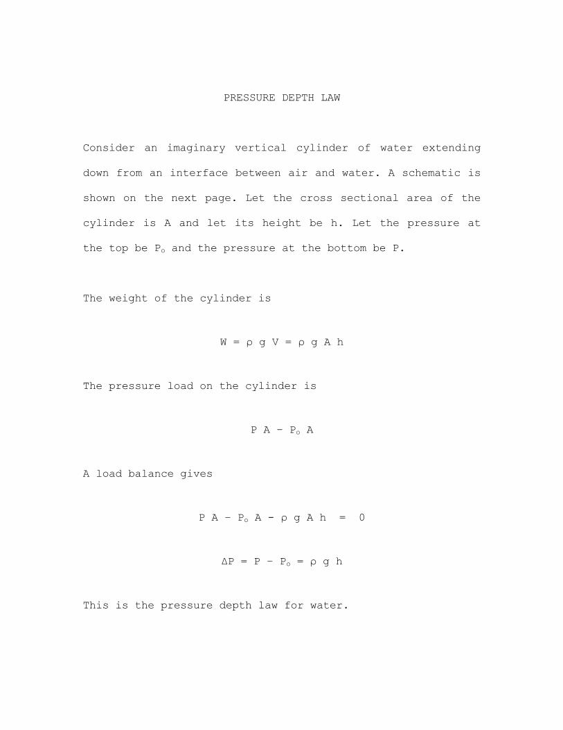
Consider an imaginary vertical cylinder of water extending
down from an interface between air and water. A schematic is
shown on the next page. Let the cross sectional area of the
cylinder is A and let its height be h. Let the pressure at
the top be Po and the pressure at the bottom be P.
The weight of the cylinder is
W = ρ g V = ρ g A h
The pressure load on the cylinder is
P A – Po A
A load balance gives
P A – Po A - ρ g A h = 0
ΔP = P – Po = ρ g h
This is the pressure depth law for water.
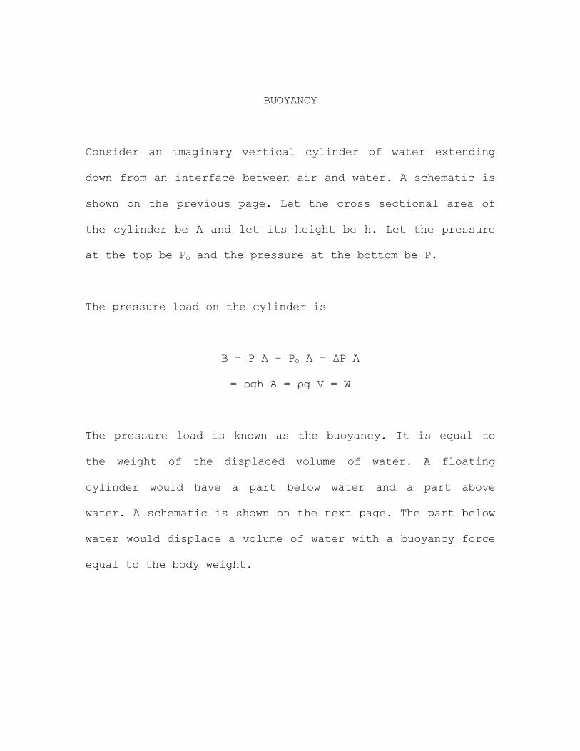
BUOYANCY
Consider an imaginary vertical cylinder of water extending
down from an interface between air and water. A schematic is
shown on the previous page. Let the cross sectional area of
the cylinder be A and let its height be h. Let the pressure
at the top be Po and the pressure at the bottom be P.
The pressure load on the cylinder is
B = P A – Po A = ΔP A
= ρgh A = ρg V = W
The pressure load is known as the buoyancy. It is equal to
the weight of the displaced volume of water. A floating
cylinder would have a part below water and a part above
water. A schematic is shown on the next page. The part below
water would displace a volume of water with a buoyancy force
equal to the body weight.
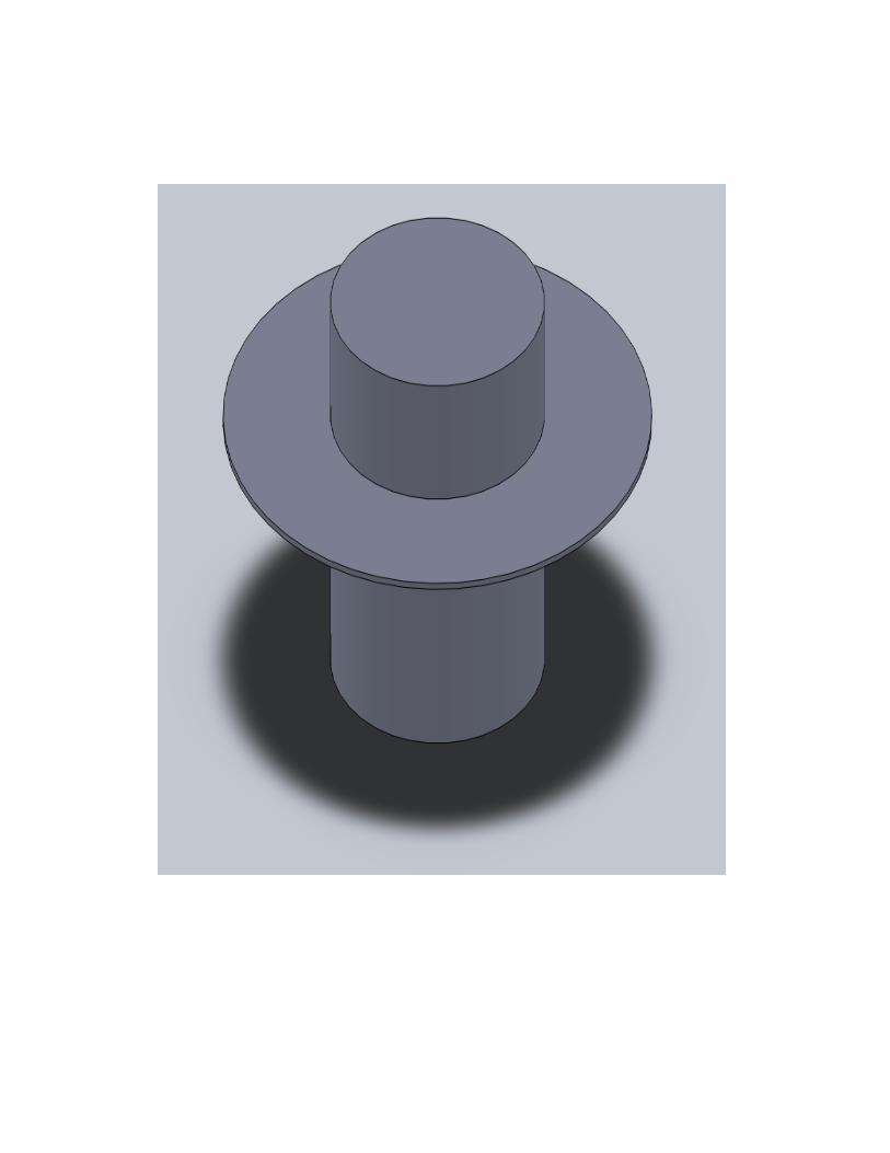
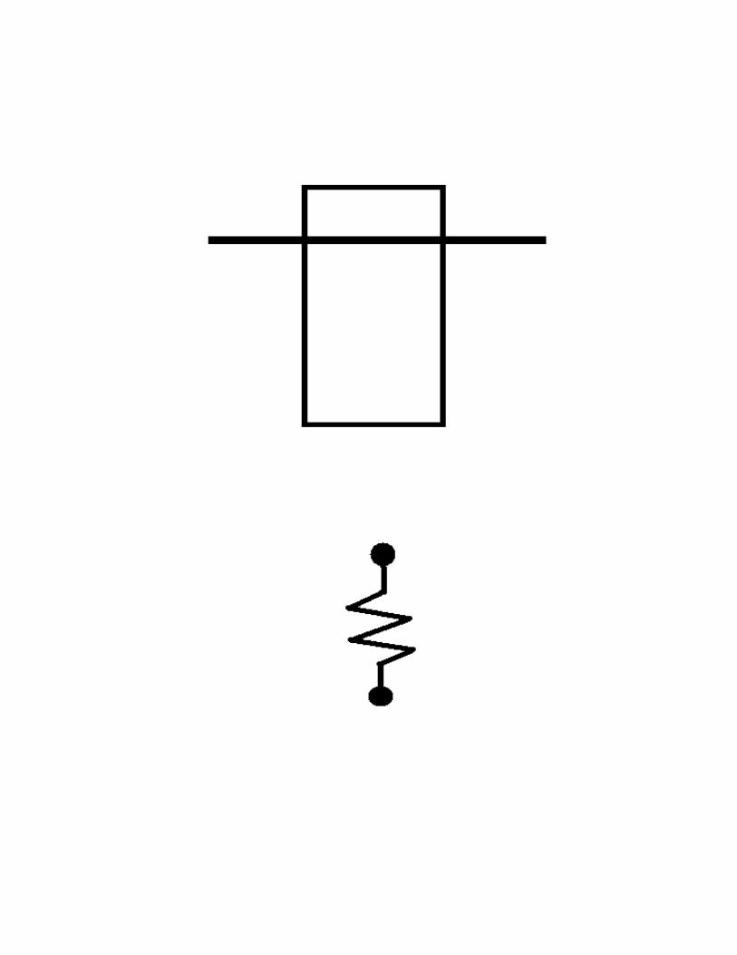
BUOYANCY SPRING
The buoyancy force can be written as
B = ρgA h
This resembles a spring
F = K x
The buoyancy spring constant is
K = ρgA
A schematic of the analogy is on the next page.
Pushing the cylinder downwards increases the buoyancy force.
It compresses the buoyancy spring. It pushes the bottom down
to a level where the pressure is higher and that creates an
increase in the force upwards.
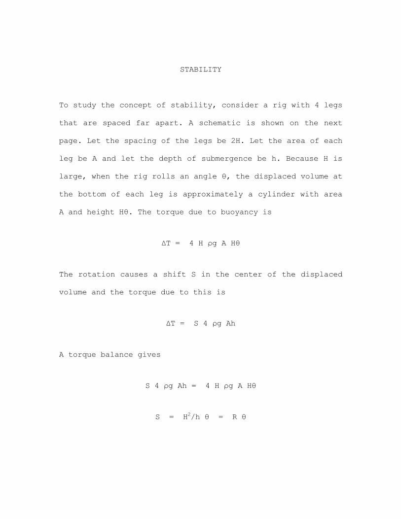
STABILITY
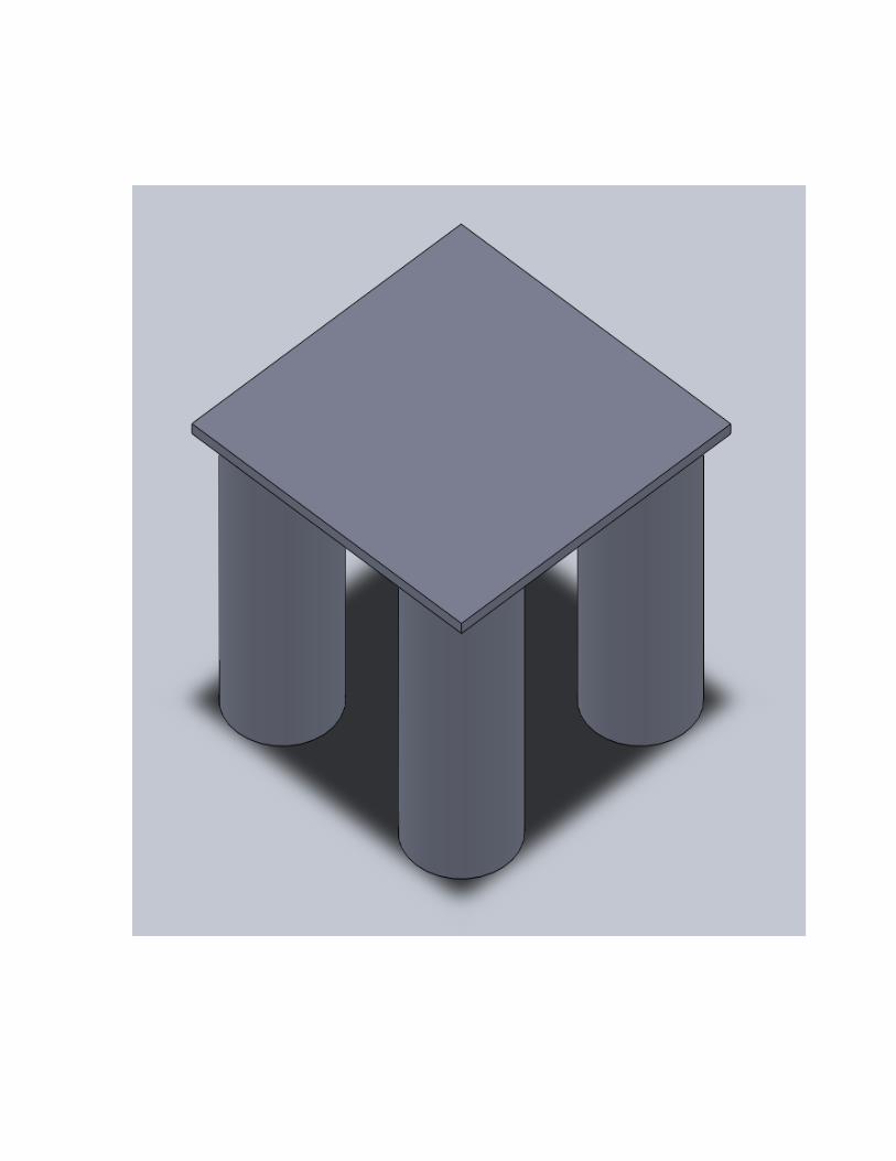
To study the concept of stability, consider a rig with 4 legs
that are spaced far apart. A schematic is shown on the next
page. Let the spacing of the legs be 2H. Let the area of each
leg be A and let the depth of submergence be h. Because H is
large, when the rig rolls an angle θ, the displaced volume at
the bottom of each leg is approximately a cylinder with area
A and height Hθ. The torque due to buoyancy is
ΔT = 4 H ρg A Hθ
The rotation causes a shift S in the center of the displaced
volume and the torque due to this is
ΔT = S 4 ρg Ah
A torque balance gives
S 4 ρg Ah = 4 H ρg A Hθ
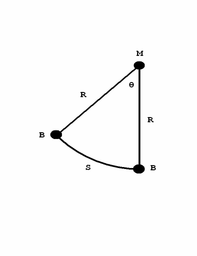
S = H2/h θ = R θ
This suggests that the center of buoyancy has moved along a
circular arc with radius R. A schematic of this shift is
shown in the sketch on the next page. The radius is known as
the metacentric radius. The center of rotation is known as
the metacenter. The line of action of the buoyancy force
always passes through this point. Knowing the location of the
metacenter allows us to locate the line of action of the
buoyancy force. If the center of gravity is below the
metacenter, the weight and buoyancy forces create a restoring
moment and the rig is stable. If the center of gravity is
above the metacenter, the weight and buoyancy forces create
an overturning moment and the rig is unstable.
FLUIDS AT REST
SUBMERGED
SURFACES
HYDRAULIC GATES
To get loads on hydraulic gates one can break its surface up
into an infinite number of infinitesimal bits of surface. The
force on an infinitesimal bit of surface is:
dF = P ds n
where n is the inward normal on the surface and P is the
pressure acting on it. The normal n is:
n = nx i + ny j + nz k
where ijk indicates unit normal vectors. The force can be
broken down into xyz components
dF = dFx i + dFy j + dFz k
= P ds nx i + P ds ny j + P ds nz k
The pressure depth law gives
P = ρg h
The total force can be obtained by integration of the
component forces over the total surface:
Fx = P nx ds Fy = P ny ds Fz = P nz ds
The total force is
F = Fx i + Fy j + Fz k
|F| = √ [ [Fx]2 + [Fx]2 + [Fx]2 ]
Moment balances give the location of the forces.
The panel method for hydraulic gates starts by subdividing
the surface of the gate into a finite number of finite size
flat panels. The pressure depth law gives the pressure at the
centroid of each panel. Pressure times panel area gives the
force at the centroid. The unit normal pointing at the panel
allows one to break the force into components. Summation
gives the total force on the gate in each direction.
Fx = P nx s Fy = P ny s Fz = P nz s
The total force is
F = Fx i + Fy j + Fz k
|F| = √ [ [Fx]2 + [Fx]2 + [Fx]2 ]
Moment balances give the location of the forces.
The pressure/weight method for hydraulic gates starts by
boxing the gate with vertical and horizontal surfaces. The
fluid within these surfaces is considered frozen to the gate.
Then the horizontal and vertical pressure forces on the box
surfaces are calculated. Force balances, which subtract the
weight frozen to the gate, then give the horizontal and
vertical forces on the gate. The total force is
F = Fx i + Fy j + Fz k
|F| = √ [ [Fx]2 + [Fx]2 + [Fx]2 ]
Moment balances give the location of the forces.
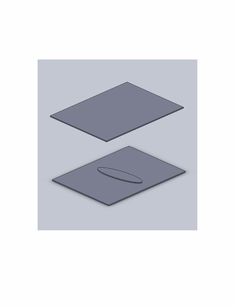
HORIZONTAL FLAT GATE
The pressure acting on the gate is
ρg H
The total force on the gate is:
ρg H A
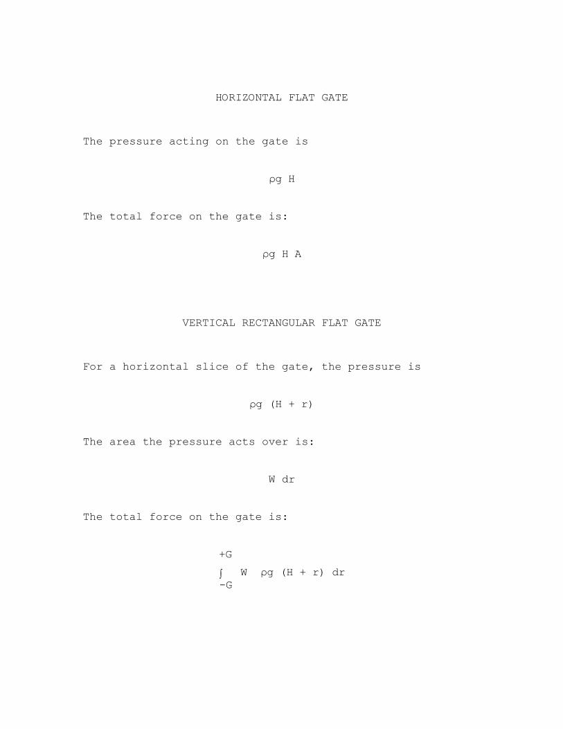
VERTICAL RECTANGULAR FLAT GATE
For a horizontal slice of the gate, the pressure is
ρg (H + r)
The area the pressure acts over is:
W dr
The total force on the gate is:
+G
W ρg (H + r) dr -G
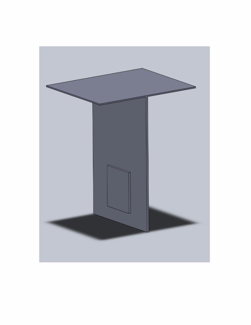
Evaluation of the integral gives
ρg H 2G W
VERTICAL CIRCULAR FLAT GATE
For a horizontal slice of the gate the pressure is
ρg (H + r)
The area the pressure acts over is:
2 √[G2-r2] dr
The total force on the gate is: +G
ρg (H + r) 2 √[G2-r2] dr
-G
Evaluation of the r integral gives
ρg H πG2
HEMISPHERICAL SIDE GATE
For a horizontal slice of the gate the pressure is
ρg (H - G Cos)
Angle is measured from top to bottom (like latitude on
earth). The area the pressure acts over is:
G d G Sin
The total vertical force on the gate is:
π
[ ρg (H - G Cos) G G Sin [-Cos] ] d 0 Evaluation of the integral gives
ρg [4/3 G3] / 2
The horizontal force on the gate is:
+π/2 π
[ ρg (H - G Cos) G G Sin [+Sin] d ] Cos d -π/2 0
Angle is measured around the slice (like longitude on
earth). Evaluation of the integral gives
ρg H G2
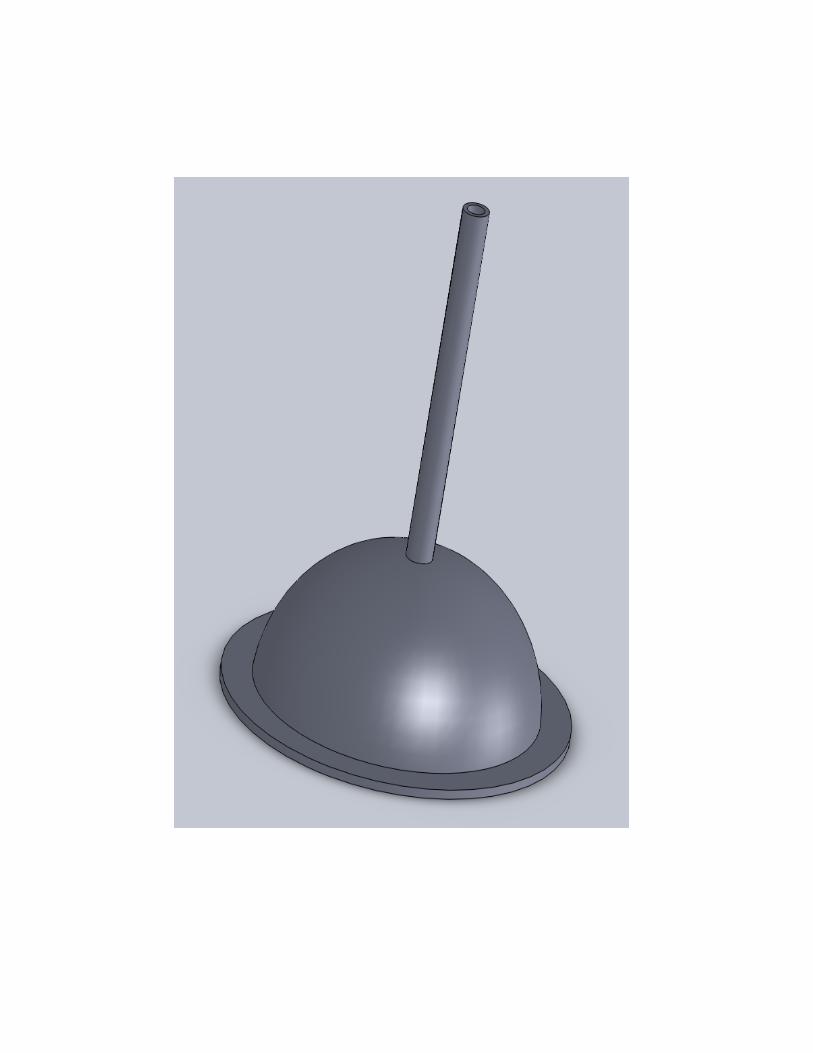
HEMISPHERICAL WATER TANK
A certain hemispherical water tank sits on a concrete
foundation. The tank diameter is 5m. At the top of the
tank, there is a small diameter vertical fill tube that is
open at the bottom to the tank and open at the top to the
atmosphere. The water level in the tube is 5m above the top
of the tank. Using the Pressure Weight Method, calculate
the vertical force in wall at the base of the tank needed
to counteract hydrostatic pressure load. Check your answer
using the Panel Method and also using Analytical
Integration. The tank wall is 1cm thick and is made out of
steel. Calculate the force on the concrete foundation.
Pressure Weight Method: Imagine the tank wall is cut just
where it joins the bottom plate. A free body diagram shows
that the force balance on tank and water above the cut
gives: wall force plus pressure force minus water weight
minus wall weight must total to zero. The forces are:
pressure force : ρg H G2
water weight : ρg [4/3 G3] / 2
wall weight : g [4 G2] t / 2
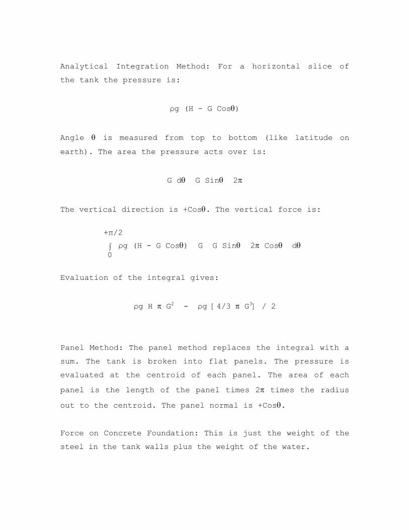
Analytical Integration Method: For a horizontal slice of
the tank the pressure is:
ρg (H - G Cos)
Angle is measured from top to bottom (like latitude on
earth). The area the pressure acts over is:
G d G Sin 2
The vertical direction is +Cos. The vertical force is:
+π/2
ρg (H - G Cos) G G Sin 2 Cos d 0
Evaluation of the integral gives:
ρg H G2 - ρg [4/3 G3] / 2
Panel Method: The panel method replaces the integral with a
sum. The tank is broken into flat panels. The pressure is
evaluated at the centroid of each panel. The area of each
panel is the length of the panel times 2 times the radius
out to the centroid. The panel normal is +Cos.
Force on Concrete Foundation: This is just the weight of the
steel in the tank walls plus the weight of the water.
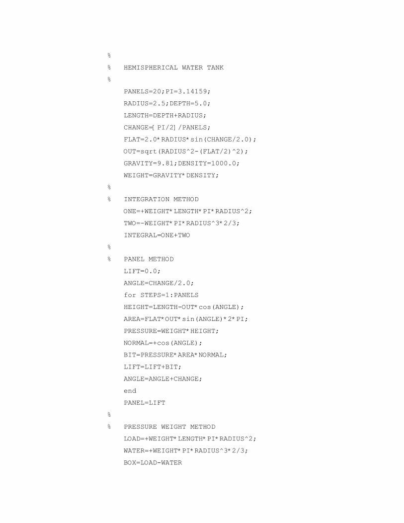
%
% HEMISPHERICAL WATER TANK
%
PANELS=20;PI=3.14159;
RADIUS=2.5;DEPTH=5.0;
LENGTH=DEPTH+RADIUS;
CHANGE=[PI/2]/PANELS;
FLAT=2.0*RADIUS*sin(CHANGE/2.0);
OUT=sqrt(RADIUS^2-(FLAT/2)^2);
GRAVITY=9.81;DENSITY=1000.0;
WEIGHT=GRAVITY*DENSITY;
%
% INTEGRATION METHOD
ONE=+WEIGHT*LENGTH*PI*RADIUS^2;
TWO=-WEIGHT*PI*RADIUS^3*2/3;
INTEGRAL=ONE+TWO
%
% PANEL METHOD
LIFT=0.0;
ANGLE=CHANGE/2.0;
for STEPS=1:PANELS
HEIGHT=LENGTH-OUT*cos(ANGLE);
AREA=FLAT*OUT*sin(ANGLE)*2*PI;
PRESSURE=WEIGHT*HEIGHT;
NORMAL=+cos(ANGLE);
BIT=PRESSURE*AREA*NORMAL;
LIFT=LIFT+BIT;
ANGLE=ANGLE+CHANGE;
end
PANEL=LIFT
%
% PRESSURE WEIGHT METHOD
LOAD=+WEIGHT*LENGTH*PI*RADIUS^2;
WATER=+WEIGHT*PI*RADIUS^3*2/3;
BOX=LOAD-WATER
FLUIDS AT REST
HYDROSTATIC
STABILITY
METACENTER
When a neutrally buoyant body is rotated, it will return to
its original orientation if buoyancy and weight create a
restoring moment. For a submerged body, this occurs when
the center of gravity is below the center of buoyancy. The
center of buoyancy will act like a pendulum pivot. For a
floating body, a restoring moment is generated when the
center of gravity is below a point known as the metacenter.
In this case, the metacenter acts like a pendulum pivot.
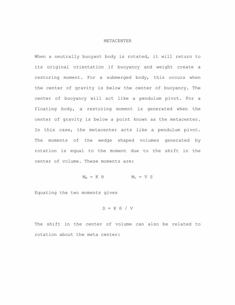
The moments of the wedge shaped volumes generated by
rotation is equal to the moment due to the shift in the
center of volume. These moments are:
MW = K θ MV = V S
Equating the two moments gives
S = K θ / V
The shift in the center of volume can also be related to
rotation about the meta center:
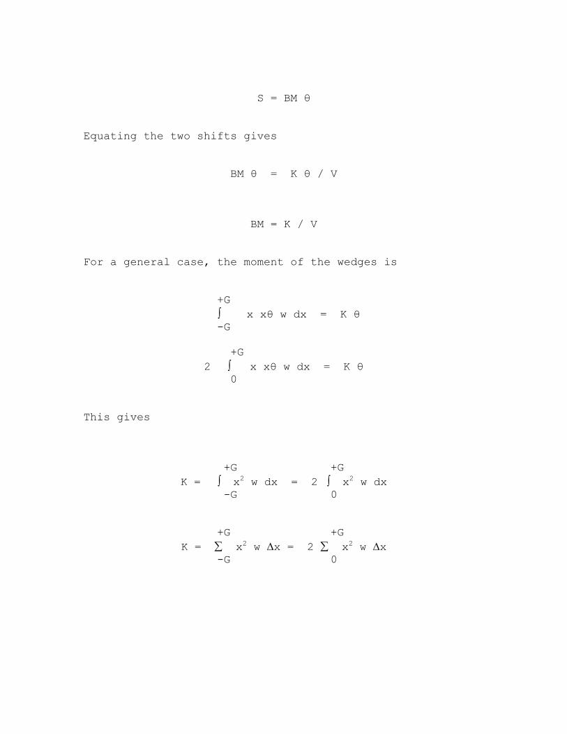
S = BM θ
Equating the two shifts gives
BM θ = K θ / V
BM = K / V
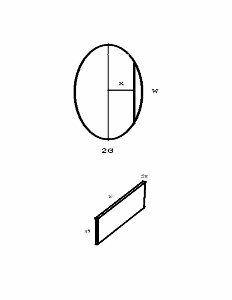
For a general case, the moment of the wedges is
+G
x xθ w dx = K θ -G +G
2 x xθ w dx = K θ 0
This gives
+G +G K = x2 w dx = 2 x2 w dx
-G 0
+G +G K = x2 w x = 2 x2 w x
-G 0
The metacenter M occurs at the intersection of two lines. One
line passes through the center of gravity or G and the center
of buoyancy or B of a floating body when it is not rotated:
the other line is a vertical line through B when the body is
rotated. Inspection of a sketch of these lines shows that, if
M is above G, gravity and buoyancy generate a restoring
moment, whereas if M is below G, gravity and buoyancy
generate an overturning moment. One finds the location of M
by finding the shift in the center of volume generated during
rotation and noting that this shift could result from a
rotation about an imaginary point which turns out to be the
metacenter. The distance between B and the center of gravity
G is BG. Geometry gives GM:
GM = BM - BG
If GM is positive, M is above G and the body is stable. If GM
is negative, M is below G and the body is unstable.

STABLE
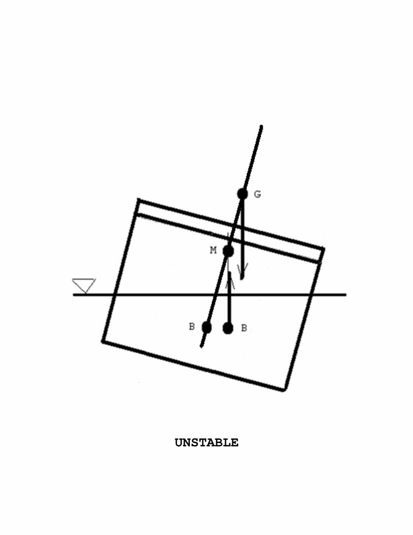
UNSTABLE
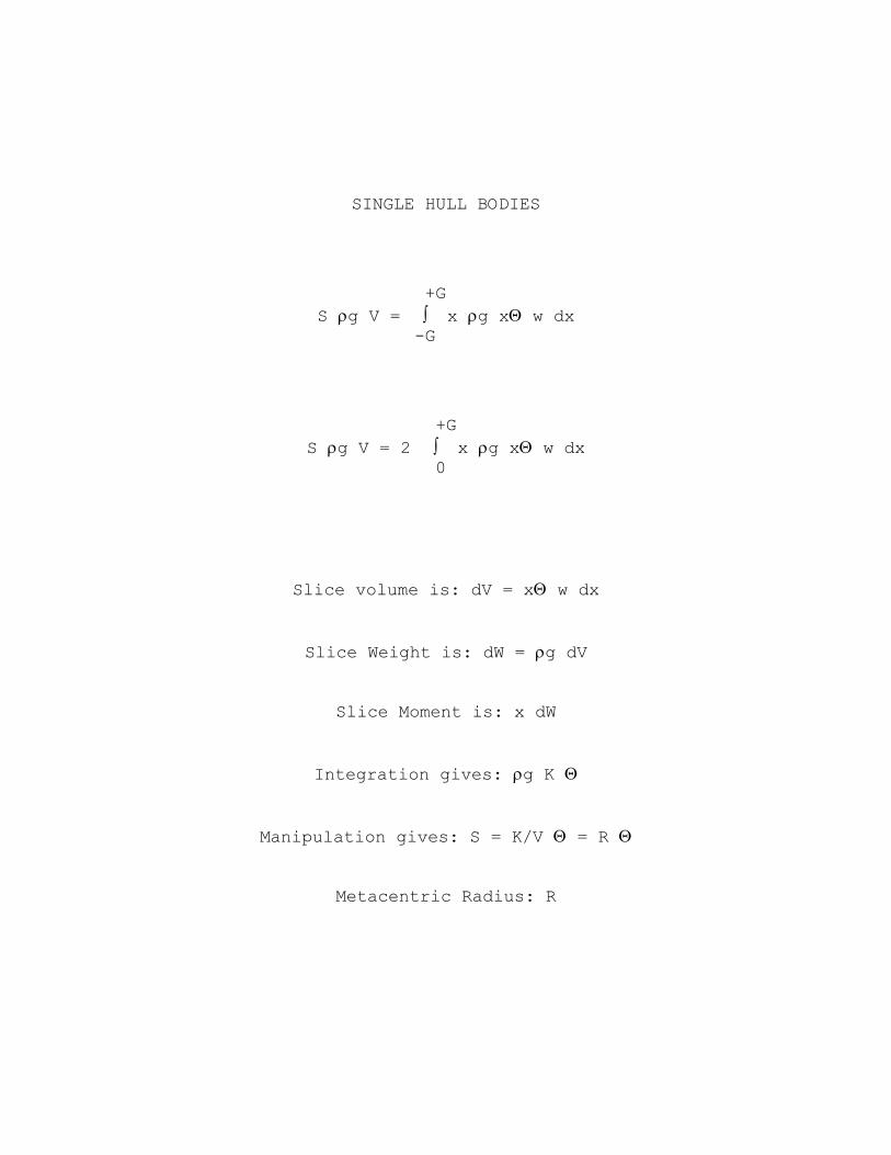
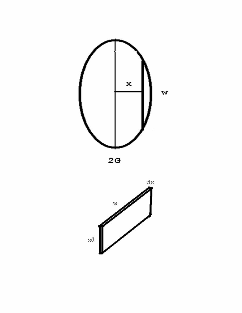
SINGLE HULL BODIES
+G S g V = x g x w dx
-G
+G S g V = 2 x g x w dx
0
Slice volume is: dV = x w dx
Slice Weight is: dW = g dV
Slice Moment is: x dW
Integration gives: g K
Manipulation gives: S = K/V = R
Metacentric Radius: R
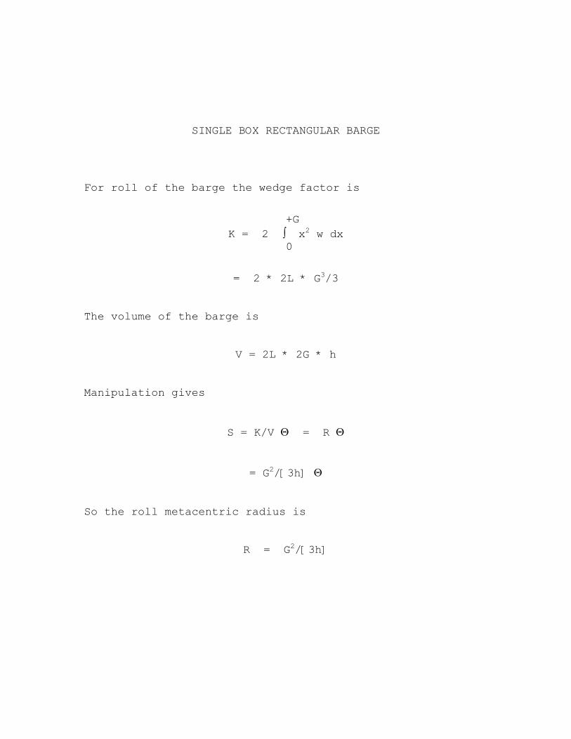
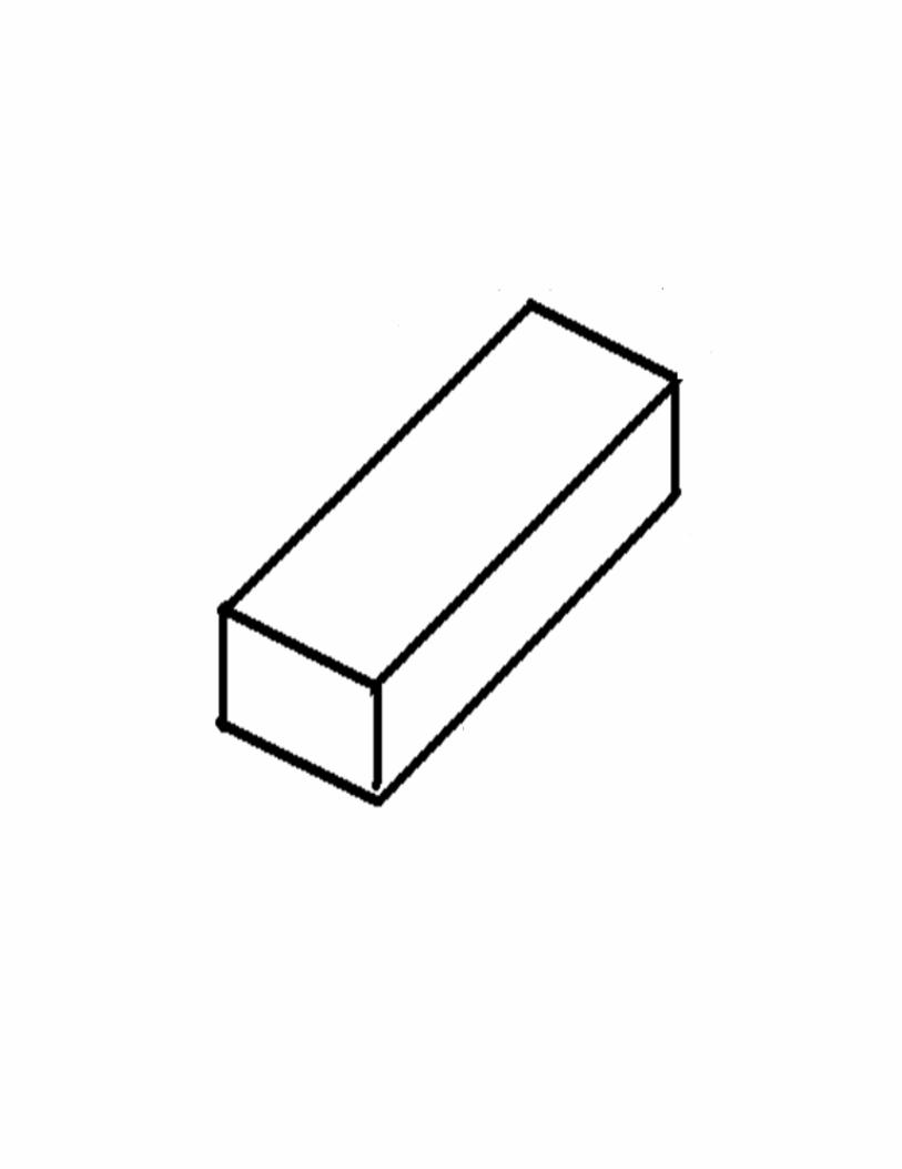
SINGLE BOX RECTANGULAR BARGE
For roll of the barge the wedge factor is
+G
K = 2 x2 w dx 0
= 2 * 2L * G3/3
The volume of the barge is
V = 2L * 2G * h
Manipulation gives
S = K/V = R
= G2/[3h]
So the roll metacentric radius is
R = G2/[3h]
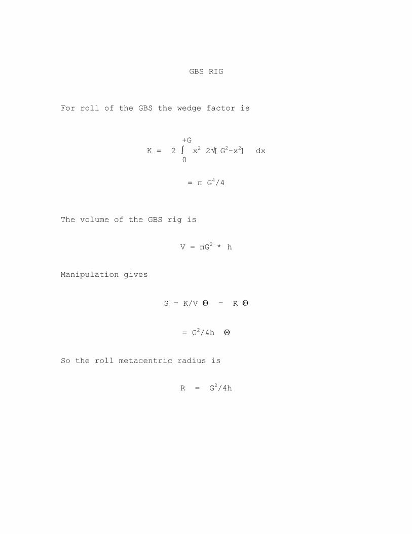
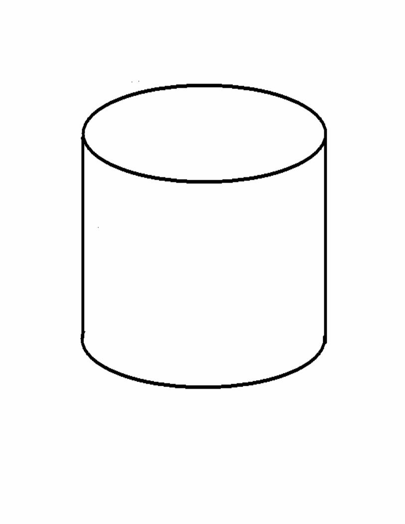
GBS RIG
For roll of the GBS the wedge factor is
+G
K = 2 x2 2√[G2-x2] dx 0
= π G4/4
The volume of the GBS rig is
V = πG2 * h
Manipulation gives
S = K/V = R
= G2/4h
So the roll metacentric radius is
R = G2/4h
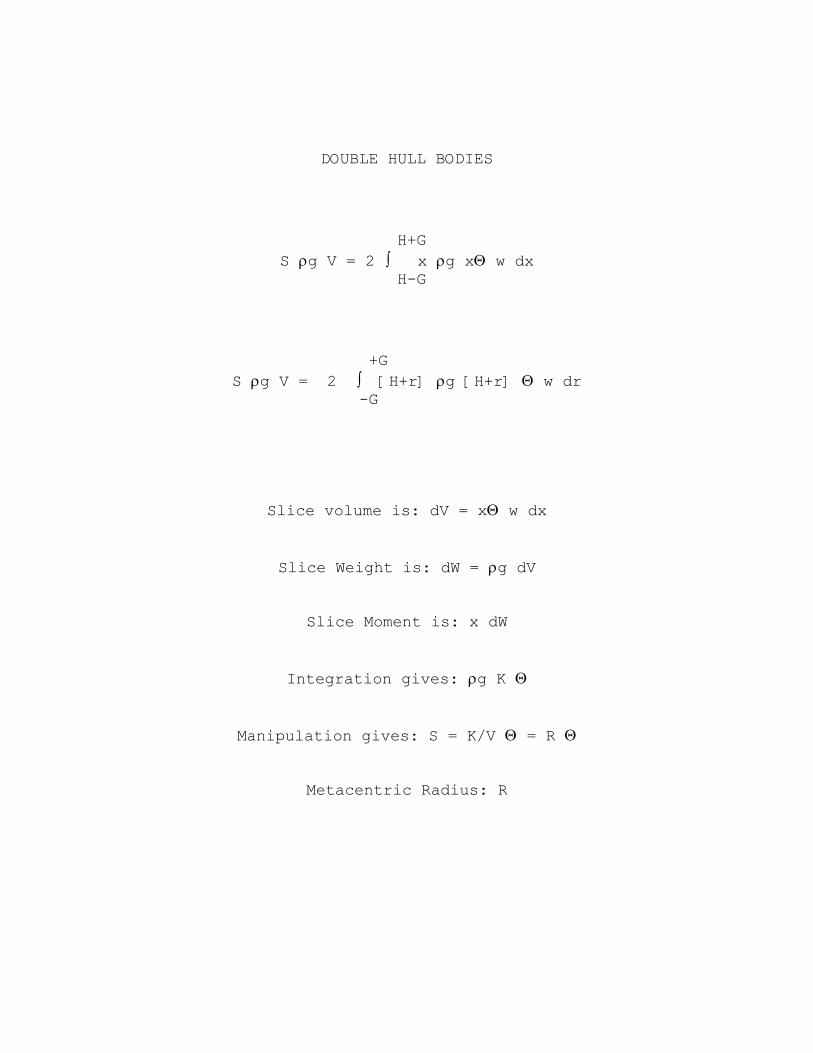
DOUBLE HULL BODIES
H+G S g V = 2 x g x w dx
H-G
+G S g V = 2 [H+r] g [H+r] w dr
-G
Slice volume is: dV = x w dx
Slice Weight is: dW = g dV
Slice Moment is: x dW
Integration gives: g K
Manipulation gives: S = K/V = R
Metacentric Radius: R
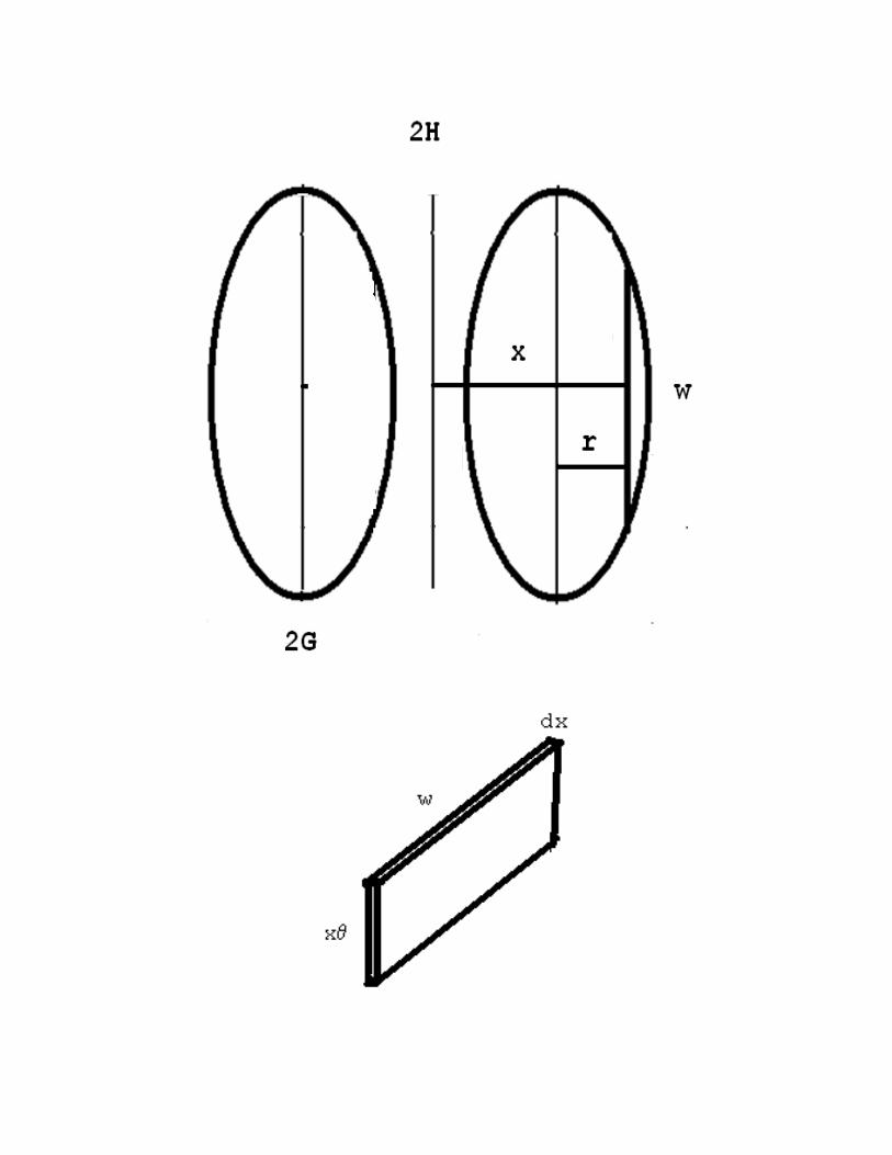
DOUBLE BOX RECTANGULAR BARGE
For roll of the barge the wedge factor is
+G
K = 2 (H+r)2 2L dr -G
= 2L (4G3/3 + 4H2G)
The volume of the barge is
V = 2 * 2L * 2G * h
Manipulation gives
S = K/V = R
= (G2/3h + H2/h)
So the roll metacentric radius is
R = G2/3h + H2/h
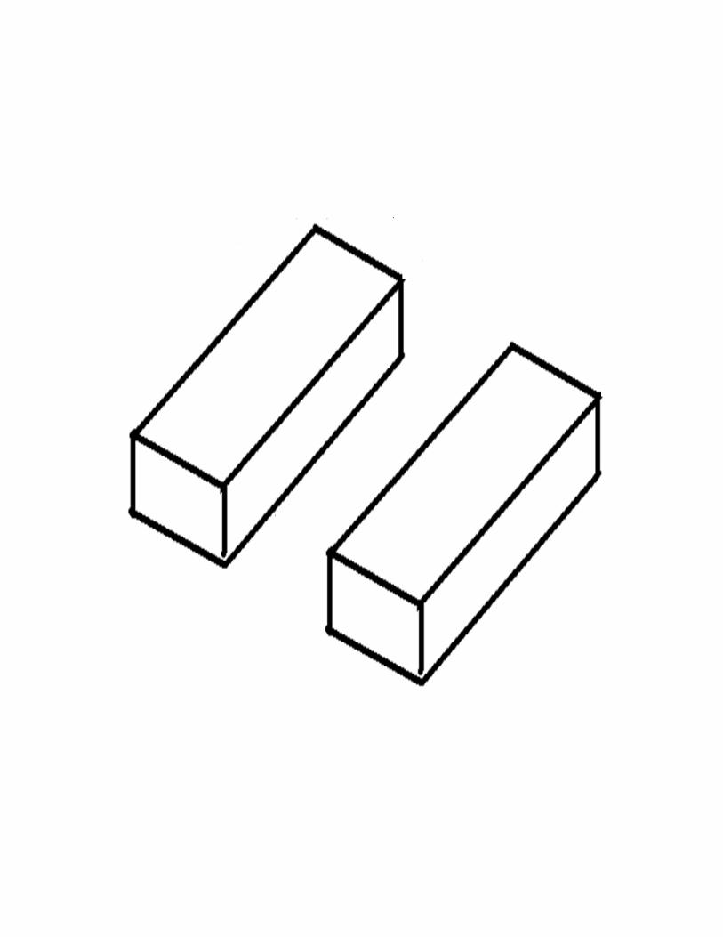
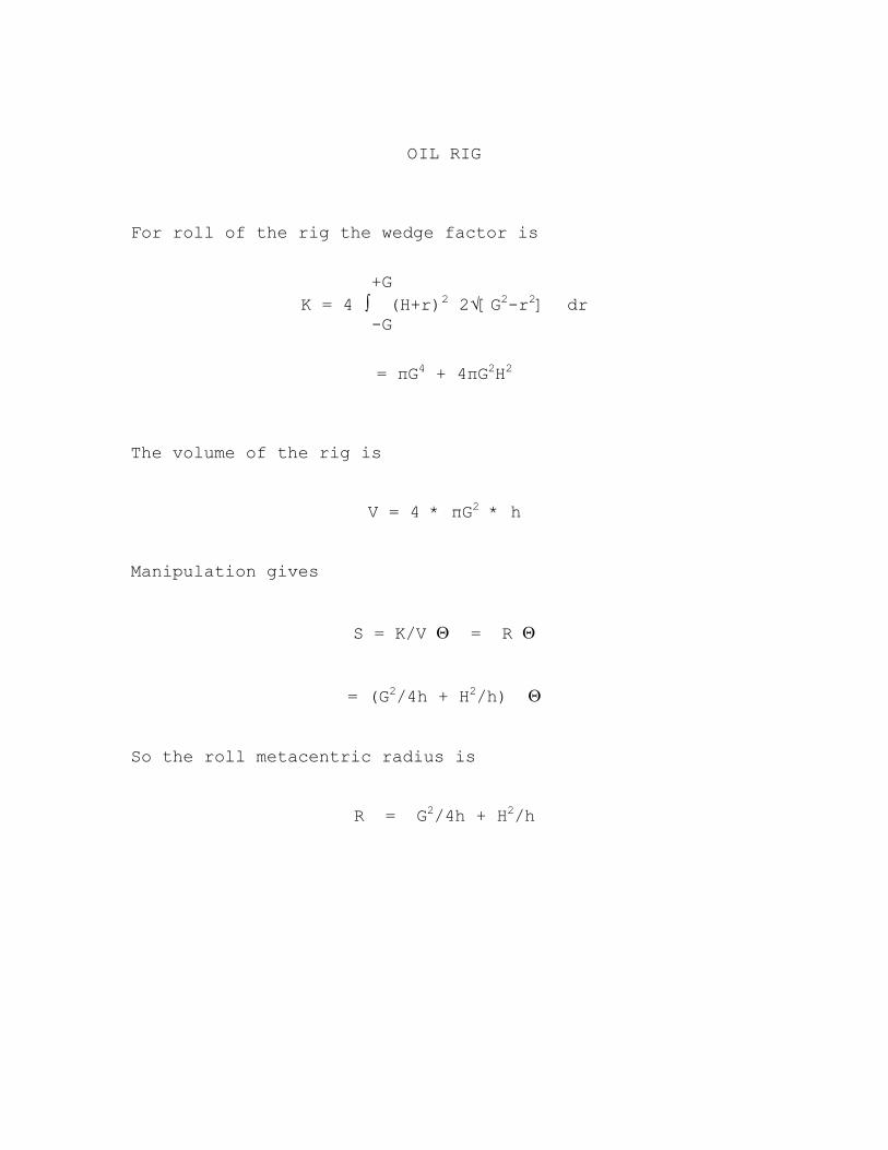
OIL RIG
For roll of the rig the wedge factor is
+G
K = 4 (H+r)2 2√[G2-r2] dr -G
= πG4 + 4πG2H2
The volume of the rig is
V = 4 * πG2 * h
Manipulation gives
S = K/V = R
= (G2/4h + H2/h)
So the roll metacentric radius is
R = G2/4h + H2/h
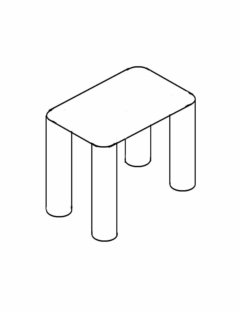
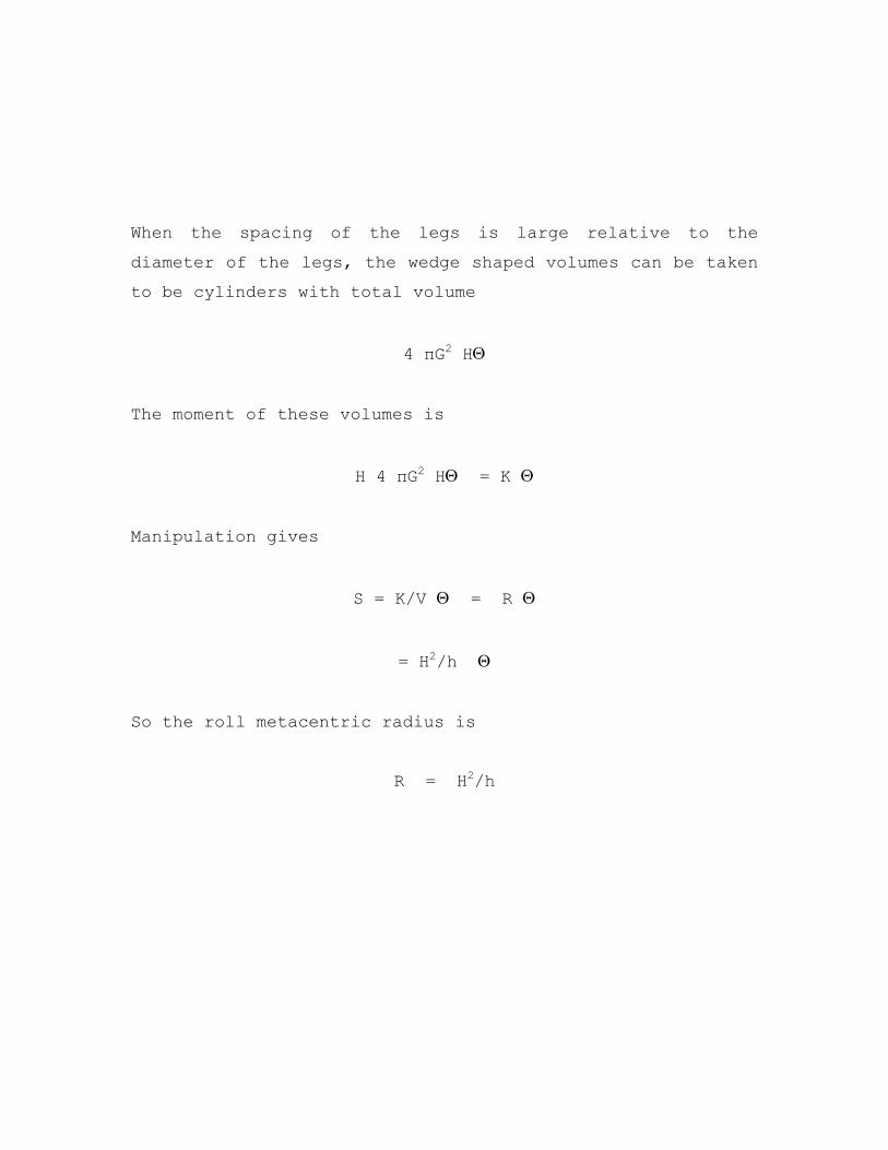
When the spacing of the legs is large relative to the
diameter of the legs, the wedge shaped volumes can be taken
to be cylinders with total volume
4 πG2 H
The moment of these volumes is
H 4 πG2 H = K
Manipulation gives
S = K/V = R
= H2/h
So the roll metacentric radius is
R = H2/h
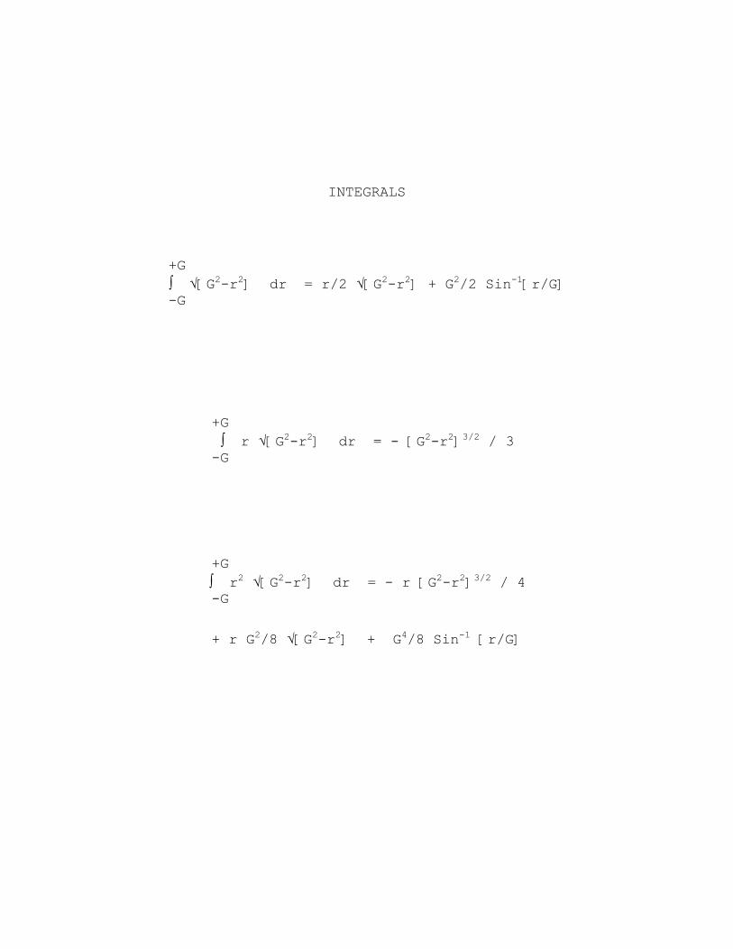
INTEGRALS
+G √[G2-r2] dr = r/2 √[G2-r2] + G2/2 Sin-1[r/G]
-G
+G r √[G2-r2] dr = - [G2-r2]3/2 / 3
-G
+G
r2 √[G2-r2] dr = - r [G2-r2]3/2 / 4 -G
+ r G2/8 √[G2-r2] + G4/8 Sin-1 [r/G]
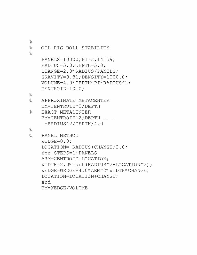
% % OIL RIG ROLL STABILITY % PANELS=10000;PI=3.14159; RADIUS=5.0;DEPTH=5.0; CHANGE=2.0*RADIUS/PANELS; GRAVITY=9.81;DENSITY=1000.0; VOLUME=4.0*DEPTH*PI*RADIUS^2; CENTROID=10.0; % % APPROXIMATE METACENTER BM=CENTROID^2/DEPTH % EXACT METACENTER BM=CENTROID^2/DEPTH .... +RADIUS^2/DEPTH/4.0 % % PANEL METHOD WEDGE=0.0; LOCATION=-RADIUS+CHANGE/2.0; for STEPS=1:PANELS ARM=CENTROID+LOCATION; WIDTH=2.0*sqrt(RADIUS^2-LOCATION^2); WEDGE=WEDGE+4.0*ARM^2*WIDTH*CHANGE; LOCATION=LOCATION+CHANGE; end BM=WEDGE/VOLUME
FLUIDS IN MOTION
CONCEPTS
OVERVIEW OF FLUID FLOWS
MOLECULAR NATURE OF LIQUIDS AND GASES
The molecules of a liquid are on average much closer together
than those in a gas. This leads to significant intermolecular
forces in a liquid and a high resistance to compression.
Intermolecular forces in a gas are much less significant and the
resistance to compression is much smaller. In a liquid,
intermolecular forces give rise to wavy molecular trajectories
whereas the lack of such forces in a gas causes trajectories to
be basically straight. In a gas, pressure is due mainly to
rebound forces associated with the high speed motion of its
molecules. In a liquid, intermolecular forces also contribute.
When pressure in a liquid, at 20oC say, is lowered sufficiently,
vapor bubbles form in it. When such bubbles collapse inside a
pump, they can damage its blades: the phenomenon is known as
cavitation. In both liquids and gases, temperature is basically
a measure of the kinetic energy of molecular motion. In a gas,
viscosity is due mainly due to the high speed random motion of
its molecules. In a flow, these cause a lateral transfer of
momentum. In a liquid, this transfer is due mainly to
intermolecular forces.
TURBULENT FLOWS
At low speeds, fluid particles move along smooth streamline
paths: motion has a laminar or layered structure. At high
speeds, particles have superimposed onto their basic streamwise
observable motion a random walk or chaotic motion. Particles
move as groups in small spinning bodies known as eddies. The
flow pattern is said to be turbulent. The small eddies in a
turbulent flow diffuse momentum. This is basically what
viscosity does in a laminar gas flow. So, to solve practical
flow problems, engineers often try to model turbulence as an
extra or eddy viscosity. Turbulent flows are too complex to deal
with analytically: one must use CFD.
BOUNDARY LAYER FLOWS
When a body moves through a viscous fluid, the fluid at its
surface moves with it. It does not slip over the surface. When a
body moves at high speed, the transition between the surface and
flow outside is known as a boundary layer. In a relative sense,
it is a very thin layer. Within it, viscosity plays a dominant
role because normal velocity gradients are very large. Gradients
are responsible for skin friction drag on things like the wings
and fuselage of aircraft. Boundary layers can separate from
surfaces and radically alter the surrounding flow pattern. This
is what happens when a wing stalls.
LOW REYNOLDS NUMBER FLOWS
When fluid moves through narrow spaces, the Reynolds Number of
the flow is very low because the gap between the spaces, which
is the characteristic dimension for such a flow, is very small.
Low Reynolds Number means that viscous forces on the fluid are
much greater than inertia forces. High pressures are needed to
push fluid through such spaces. Hydrodynamic lubrication devices
use the high pressures to support loads.
IDEAL OR POTENTIAL FLOWS
Well away from fluid boundaries, viscous forces are often small
relative to inertia and pressure forces. Flows without viscosity
are known as ideal or potential flows. The governing equations
for such flows give a very accurate description of water waves.
When they are applied to flow around a wing, they predict zero
lift! Also, they give an unrealistic flow pattern around the
wing. Something can be added to the formulation which mimics
viscosity. When this is done, lift and flow patterns become
realistic. So, without viscosity, planes could not fly!
COMPRESSIBLE FLOWS
When a fluid moves at around the local speed of sound, fluid
compressibility becomes important. This is especially the case
for high speed gas flows such as that in a rocket nozzle.
Subsonic flows have a local flow speed which is everywhere less
than the local speed of sound. Most commercial jets fly at speed
around 0.75 times the local speed of sound. Aircraft are said to
fly at supersonic speeds when the local flow speed is everywhere
greater than the local speed of sound. When one flies at
supersonic speeds, the air ahead of it is unaware it is coming
because disturbance waves generated by the craft are all swept
downstream by the high speed flow: none can propagate upstream.
Shock waves form near the craft: one is usually attached to its
nose. Shock waves are very thin surfaces in a flow, usually only
around 0.00025mm thick, across which there is a large increase
in temperature and pressure. They cause very high drag.
UNSTEADY FLOWS IN PIPE NETWORKS
Unsteady flow in pipe networks can be caused by a number of
factors. A turbomachine with blades can send pressure waves down a
pipe. If the period of these waves matches a natural period of the
pipe wave speed resonance develops. Sudden changes in valves or
turbomachines cause pressure waves in pipe networks. These can
cause pipes to explode or implode. In some cases interaction
between pipes and devices is such that oscillations develop
automatically. Examples include oscillations set up by leaky
valves and those set up by slow turbomachine controllers.
FLOWS IN STREAM TUBES
CONSERVATION LAWS IN INTEGRAL FORM
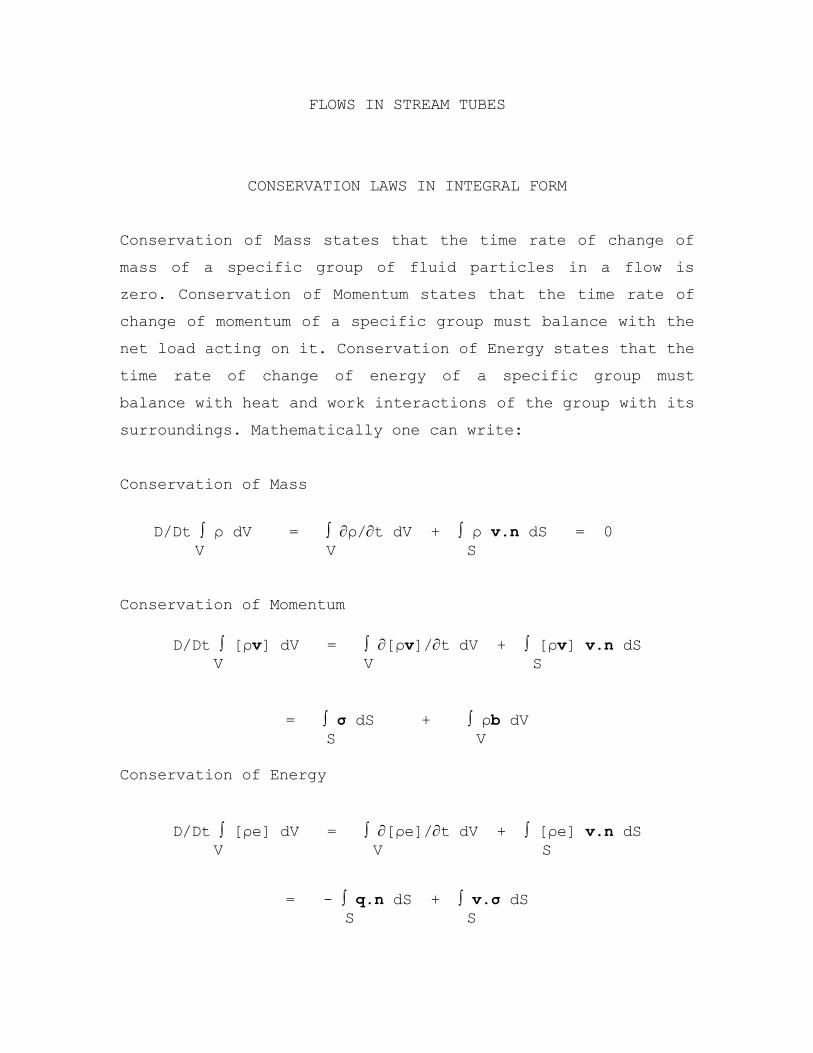
Conservation of Mass states that the time rate of change of
mass of a specific group of fluid particles in a flow is
zero. Conservation of Momentum states that the time rate of
change of momentum of a specific group must balance with the
net load acting on it. Conservation of Energy states that the
time rate of change of energy of a specific group must
balance with heat and work interactions of the group with its
surroundings. Mathematically one can write:
Conservation of Mass
D/Dt ρ dV = ρ/t dV + ρ v.n dS = 0
V V S
Conservation of Momentum
D/Dt [ρv] dV = [ρv]/t dV + [ρv] v.n dS
V V S
= σ dS + ρb dV
S V
Conservation of Energy
D/Dt [ρe] dV = [ρe]/t dV + [ρe] v.n dS
V V S
= - q.n dS + v.σ dS
S S
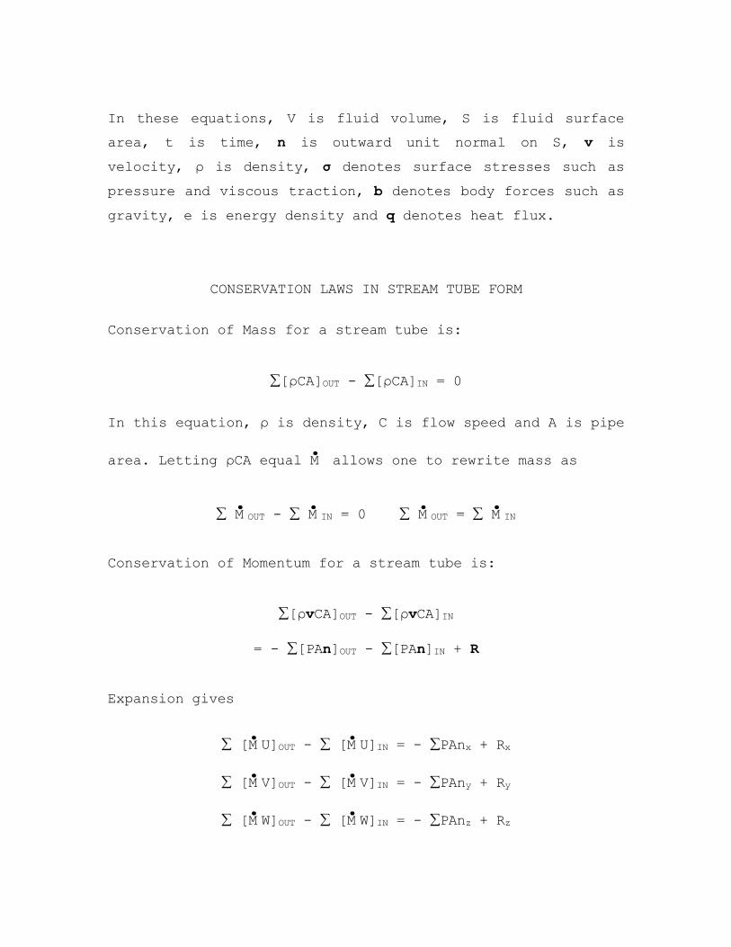
In these equations, V is fluid volume, S is fluid surface
area, t is time, n is outward unit normal on S, v is
velocity, ρ is density, σ denotes surface stresses such as
pressure and viscous traction, b denotes body forces such as
gravity, e is energy density and q denotes heat flux.
CONSERVATION LAWS IN STREAM TUBE FORM
Conservation of Mass for a stream tube is:
[ρCA]OUT - [ρCA]IN = 0
In this equation, ρ is density, C is flow speed and A is pipe
area. Letting ρCA equal M.
allows one to rewrite mass as
M.
OUT - M.
IN = 0 M.
OUT = M.
IN
Conservation of Momentum for a stream tube is:
[ρvCA]OUT - [ρvCA]IN
= - [PAn]OUT - [PAn]IN + R
Expansion gives
[M.U]OUT - [M
.U]IN = - PAnx + Rx
[M.V]OUT - [M
.V]IN = - PAny + Ry
[M.W]OUT - [M
.W]IN = - PAnz + Rz
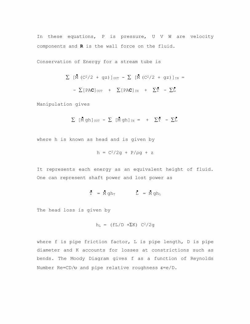
In these equations, P is pressure, U V W are velocity
components and R is the wall force on the fluid.
Conservation of Energy for a stream tube is
[M.(C2/2 + gz)]OUT - [M
.(C2/2 + gz)]IN =
- [PAC]OUT + [PAC]IN + T.
- L.
Manipulation gives
[M.gh]OUT - [M
.gh]IN = + T
. - L.
where h is known as head and is given by
h = C2/2g + P/ρg + z
It represents each energy as an equivalent height of fluid.
One can represent shaft power and lost power as
T.
= M.ghT L
. = M.ghL
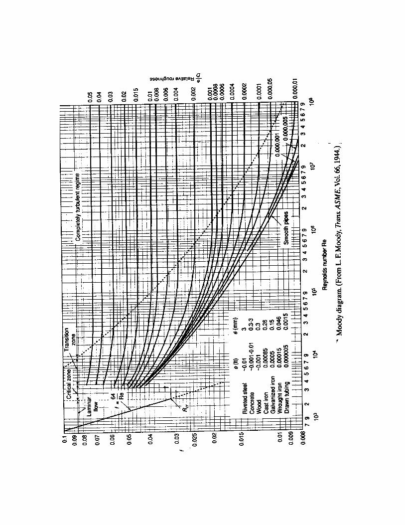
The head loss is given by
hL = (fL/D +K) C2/2g
where f is pipe friction factor, L is pipe length, D is pipe
diameter and K accounts for losses at constrictions such as
bends. The Moody Diagram gives f as a function of Reynolds
Number Re=CD/ and pipe relative roughness =e/D.
BERNOULLI EQUATION
When there is no shaft work and friction is insignificant,
conservation of energy for a stream tube shows that hOUT is
equal to hIN, which implies that h is constant:
C2/2g + P/ρg + z = K
This equation is known as the Bernoulli Equation. It can also
be derived from conservation of momentum. For a short stream
tube, a force balance gives:
DC/Dt = (C/t + CC/s) = - P/s - g z/s
For steady flow this becomes
CdC/ds = d[C2/2]/ds = - dP/ds - g dz/ds
Integration of this gives the Bernoulli equation:
C2/2 + P/ + gz =
This equation shows that, when pressure goes down in a
flow, speed goes up and visa versa. From an energy
perspective, flow work causes the speed changes. From a
momentum perspective, it is due to pressure forces.
SYSTEM DEMAND
For a system where a pipe connects two reservoirs, the head H
versus flow Q system demand equation has the form:
H = X + Y Q2
X = Δ [P/ρg + z] Y = [fL/D + K]/[2gA2]
X accounts for pressure and height changes between the
reservoirs and Y accounts for losses along the pipe.
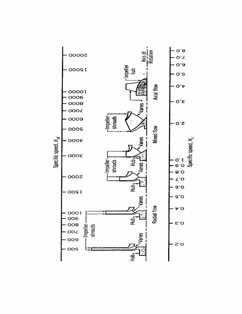
PUMP SELECTION
To pick a pump, one first calculates the specific speed N
based on the system operating point. This is a nondimensional
number which does not have pump size in it:
N = [N Q]/[H3/4]
This allows one to pick the appropriate type of pump. Axial
pumps have high Q but low H which gives them high N. Radial
pumps have lower Q but higher H which gives them lower N.
Positive Displacement pumps have the lowest Q but highest H
which gives them the lowest N. Next one scans pump catalogs
of the type indicated by specific speed and picks the size of
pump that will meet the system demand, while it is operating
at its best efficiency point (BEP) or best operating point
(BOP). Finally, to prevent cavitation, the pump is located in
the system at a point where it has the Net Positive Suction
Head or NPSH recommended by the manufacturer:
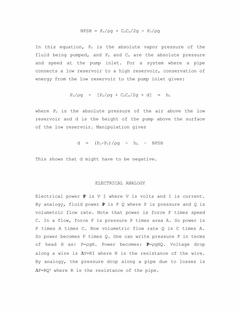
NPSH = Ps/ρg + CsCs/2g - Pv/ρg
In this equation, Pv is the absolute vapor pressure of the
fluid being pumped, and Ps and Cs are the absolute pressure
and speed at the pump inlet. For a system where a pipe
connects a low reservoir to a high reservoir, conservation of
energy from the low reservoir to the pump inlet gives:
Po/ρg - [Ps/ρg + CsCs/2g + d] = hL
where Po is the absolute pressure of the air above the low
reservoir and d is the height of the pump above the surface
of the low reservoir. Manipulation gives
d = (Po-Pv)/ρg - hL – NPSH
This shows that d might have to be negative.
ELECTRICAL ANALOGY
Electrical power P is V I where V is volts and I is current.
By analogy, fluid power P is P Q where P is pressure and Q is
volumetric flow rate. Note that power is force F times speed
C. In a flow, force F is pressure P times area A. So power is
P times A times C. Now volumetric flow rate Q is C times A.
So power becomes P times Q. One can write pressure P in terms
of head H as: P=ρgH. Power becomes: P=ρgHQ. Voltage drop
along a wire is V=RI where R is the resistance of the wire.
By analogy, the pressure drop along a pipe due to losses is
P=RQ2 where R is the resistance of the pipe.
FLUIDS IN MOTION
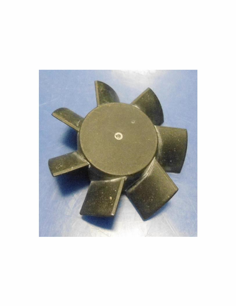
TURBOMACHINES
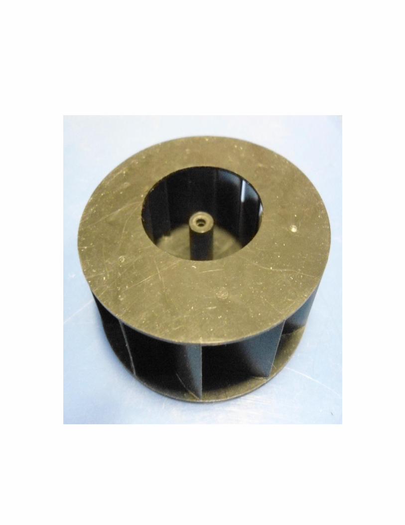
TURBOMACHINE POWER
Swirl is the only component of fluid velocity that has a
moment arm around the axis of rotation or shaft of a
turbomachine. Because of this, it is the only one that can
contribute to shaft power. The shaft power equation is:
P = Δ [T ω] = Δ [ρQ VT R ω]
The swirl or tangential component of fluid velocity is VT.
The symbol Δ indicates we are looking at changes from inlet
to outlet. The tangential momentum at an inlet or an outlet
is ρQ VT. Multiplying momentum by moment arm R gives the
torque T. Multiplying torque by the speed ω gives the power
P. The power equation is good for pumps and turbines. Power
is absorbed at an inlet and expelled at an outlet. If the
outlet power is greater than the inlet power, then the
machine is a pump. If the outlet power is less than the inlet
power, then the machine is a turbine. Geometry can be used to
connect VT to the flow rate Q and the rotor speed ω.
Theoretical analysis of turbomachines makes use of a number
of velocities. These are: the tangential flow velocity VT;
the normal flow velocity VN; the blade or bucket velocity VB;
the relative velocity VR; the jet velocity VJ.
ELECTRICAL ANALOGY
Electrical power P is V I where V is volts and I is current.
By analogy, fluid power P is P Q where P is pressure and Q is
volumetric flow rate. Note that power is force F times speed
C. In a flow, force F is pressure P times area A. So power is
P times A times C. Now volumetric flow rate Q is C times A.
So power becomes P times Q. One can write pressure P in terms
of head H as: P=ρgH. Power becomes: P=ρgHQ. Voltage drop
along a wire is V=RI where R is the resistance of the wire.
By analogy, the pressure drop along a pipe due to losses is
P=RQ2 where R is the resistance of the pipe.
TURBOMACHINE SCALING LAWS
Scaling laws allow us to predict prototype behavior from
model data. Generally the model and prototype must look the
same. This is known as geometric similitude. The flow
patterns at both scales must also look the same. This is
known as kinematic or motion similitude. Finally, certain
force ratios in the flow must be the same at both scales.
This is known as kinetic or dynamic similitude. Sometimes
getting all force ratios the same is impossible and one
must use engineering judgement to resolve the issue.
SCALING LAWS FOR TURBINES
For turbines, we are interested mainly in the power of the
device as a function of its rotational speed. The simplest
way to develop a nondimensional power is to divide power P
by something which has the units of power. The power in a
flow is equal to its dynamic pressure P times its
volumetric flow rate Q:
P Q
So, we can define a power coefficient CP:
CP = P / [P Q]
To develop a nondimensional version of the rotational speed
of the turbine, we can divide the tip speed of the blades
R by the flow speed U, which is usually equal to a jet
speed VJ. So, we can define a speed coefficient CS:
CS = R / VJ
SCALING LAWS FOR PUMPS
For a pump, it is customary to let N be the rotor RPM and D
be the rotor diameter. All flow speeds U scale as ND and all
areas A scale as D2. Pressures are set by the dynamic
pressure ρU2/2. Ignoring constants, one can define a
reference pressure [ρN2D2] and a reference flow [ND3]. Since
fluid power is just pressure times flow, one can also define
a reference power [ρN3D5]. Dividing dimensional quantities by
reference quantities gives the scaling laws:
Pressure Coefficient CP = P / [ρN2D2]
Flow Coefficient CQ = Q / [ND3]
Power Coefficient CP = P / [ρN3D5]
On the pressure versus flow characteristic of a pump, there
is a best efficiency point (BEP) or best operating point
(BOP). For geometrically similar pumps that have the same
operating point on the CP versus CQ curve, the coefficients
show that if D is doubled, P increases 4 fold, Q increases 8
fold and P increases 32 fold, whereas if N is doubled, P
increases 4 fold, Q doubles and P increases 8 fold.
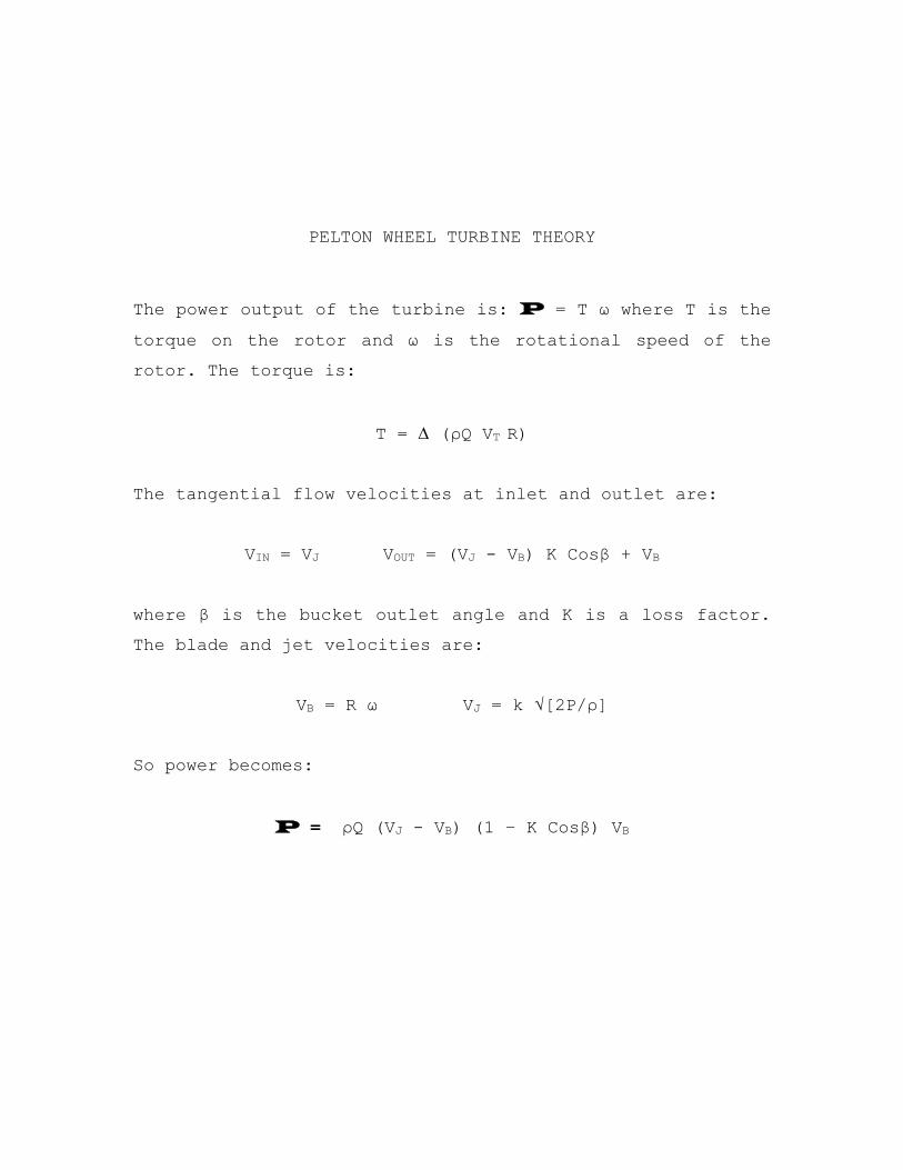
PELTON WHEEL TURBINE THEORY
The power output of the turbine is: P = T ω where T is the
torque on the rotor and ω is the rotational speed of the
rotor. The torque is:
T = (ρQ VT R)
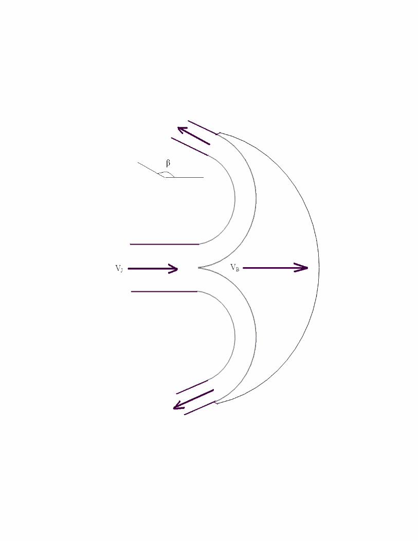
The tangential flow velocities at inlet and outlet are:
VIN = VJ VOUT = (VJ - VB) K Cosβ + VB
where β is the bucket outlet angle and K is a loss factor.
The blade and jet velocities are:
VB = R ω VJ = k √[2P/ρ]
So power becomes:
P = ρQ (VJ - VB) (1 – K Cosβ) VB
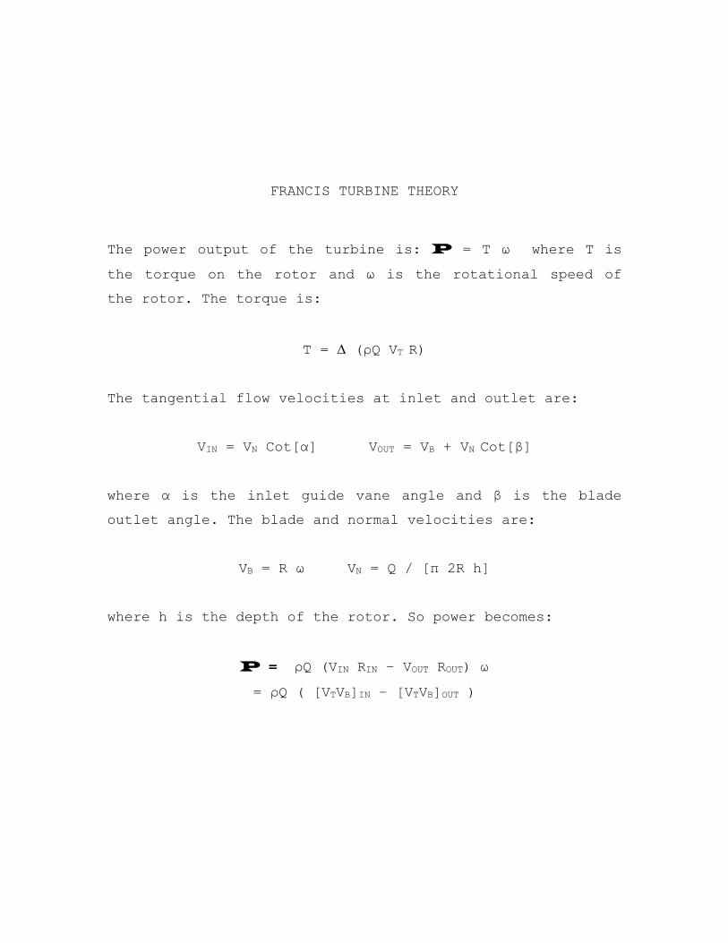
FRANCIS TURBINE THEORY
The power output of the turbine is: P = T ω where T is
the torque on the rotor and ω is the rotational speed of
the rotor. The torque is:
T = (ρQ VT R)
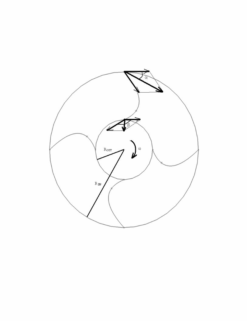
The tangential flow velocities at inlet and outlet are:
VIN = VN Cot[α] VOUT = VB + VN Cot[β]
where α is the inlet guide vane angle and β is the blade
outlet angle. The blade and normal velocities are:
VB = R ω VN = Q / [π 2R h]
where h is the depth of the rotor. So power becomes:
P = ρQ (VIN RIN – VOUT ROUT) ω
= ρQ ( [VTVB]IN – [VTVB]OUT )
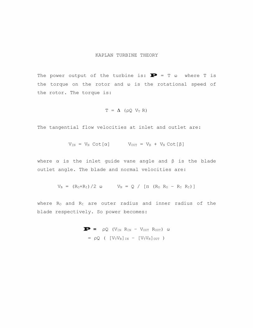
KAPLAN TURBINE THEORY
The power output of the turbine is: P = T ω where T is
the torque on the rotor and ω is the rotational speed of
the rotor. The torque is:
T = (ρQ VT R)
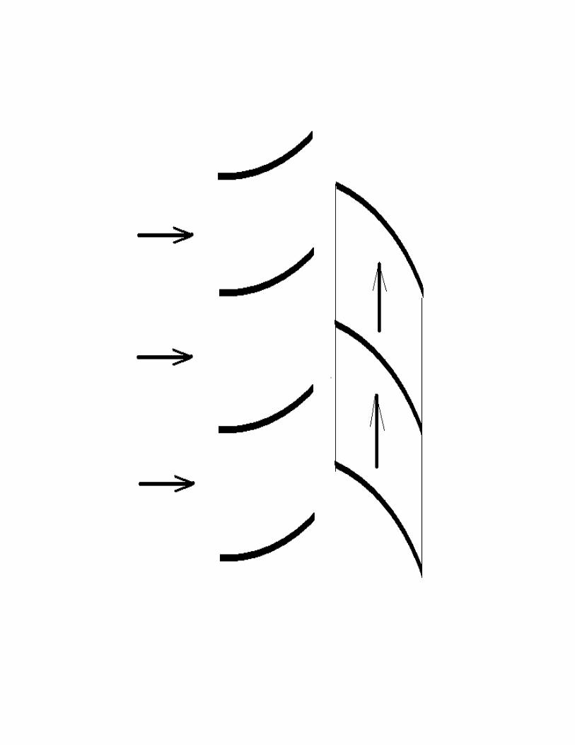
The tangential flow velocities at inlet and outlet are:
VIN = VN Cot[α] VOUT = VB + VN Cot[β]
where α is the inlet guide vane angle and β is the blade
outlet angle. The blade and normal velocities are:
VB = (RO+RI)/2 ω VN = Q / [π (RO RO – RI RI)]
where RO and RI are outer radius and inner radius of the
blade respectively. So power becomes:
P = ρQ (VIN RIN – VOUT ROUT) ω
= ρQ ( [VTVB]IN – [VTVB]OUT )
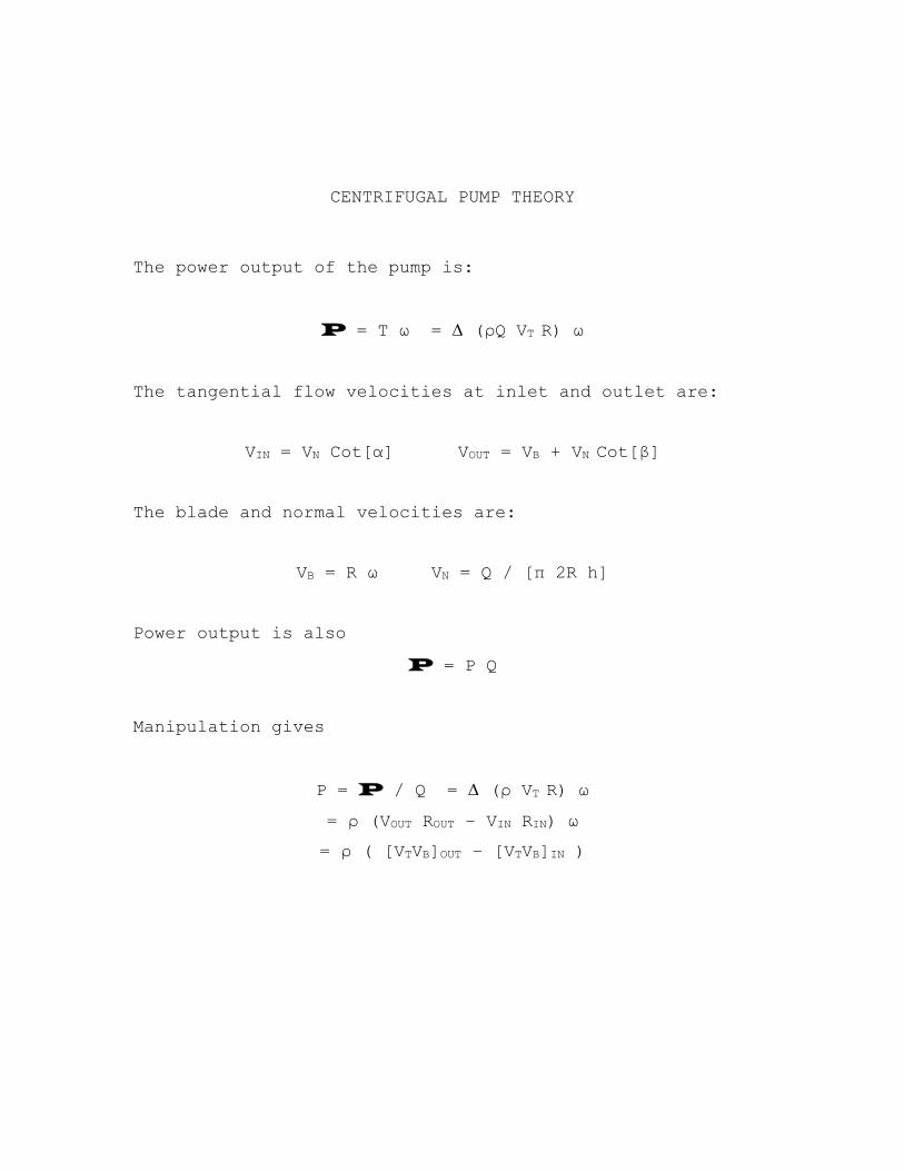
CENTRIFUGAL PUMP THEORY
The power output of the pump is:
P = T ω = (ρQ VT R) ω
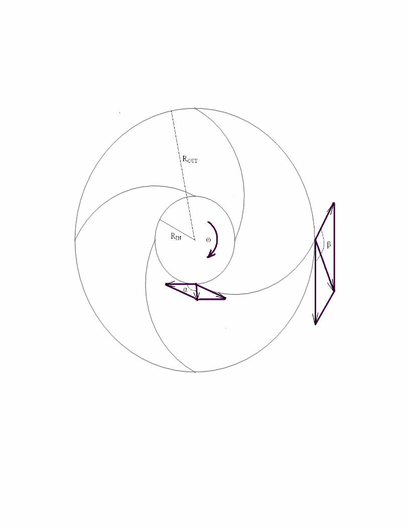
The tangential flow velocities at inlet and outlet are:
VIN = VN Cot[α] VOUT = VB + VN Cot[β]
The blade and normal velocities are:
VB = R ω VN = Q / [π 2R h]
Power output is also
P = P Q
Manipulation gives
P = P / Q = (ρ VT R) ω
= ρ (VOUT ROUT – VIN RIN) ω
= ρ ( [VTVB]OUT – [VTVB]IN )
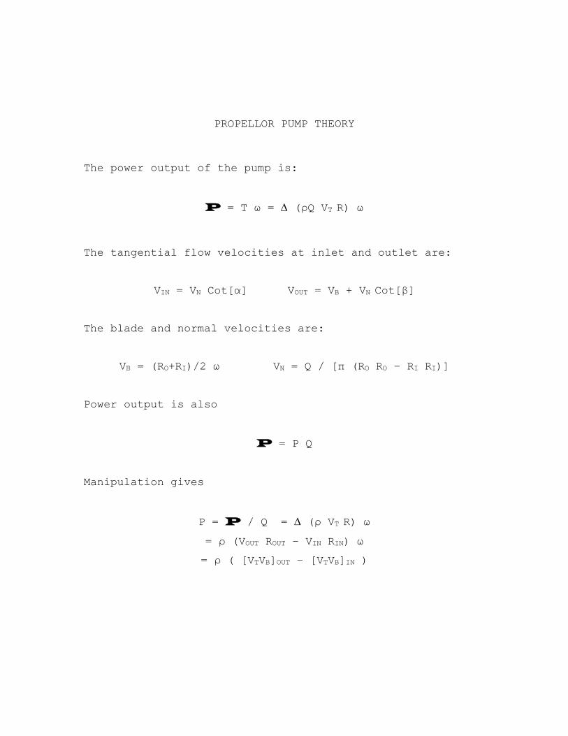
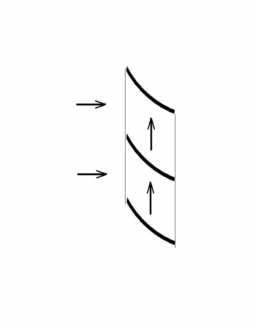
PROPELLOR PUMP THEORY
The power output of the pump is:
P = T ω = (ρQ VT R) ω
The tangential flow velocities at inlet and outlet are:
VIN = VN Cot[α] VOUT = VB + VN Cot[β]
The blade and normal velocities are:
VB = (RO+RI)/2 ω VN = Q / [π (RO RO – RI RI)]
Power output is also
P = P Q
Manipulation gives
P = P / Q = (ρ VT R) ω
= ρ (VOUT ROUT – VIN RIN) ω
= ρ ( [VTVB]OUT – [VTVB]IN )
FLUIDS IN MOTION
SCALING
LAWS
PREAMBLE
Scaling laws allow us to predict prototype behavior from
model data. Generally the model and prototype must look the
same. This is known as geometric similitude. The flow
patterns at both scales must also look the same. This is
known as kinematic or motion similitude. Finally, certain
force ratios in the flow must be the same at both scales.
This is known as kinetic or dynamic similitude. Sometimes
getting all force ratios the same is impossible and one must
use engineering judgement to resolve the issue.
The simplest way to derive scaling laws is to use common
sense. If you need to develop a nondimensional power
coefficient, you need to divide power by a reference power.
The reference power could be based on things like the
properties of the fluid and conditions imposed by the
surroundings. One could also derive the scaling laws using a
more formal procedure known as the Method of Indices. Most
fluids texts call this the Buckingham π Theorem. For this,
the variables and parameters of interest are divided into
primary and secondary categories. When using the Buckingham
π Theorem, each nondimensional coefficient is known as a π.
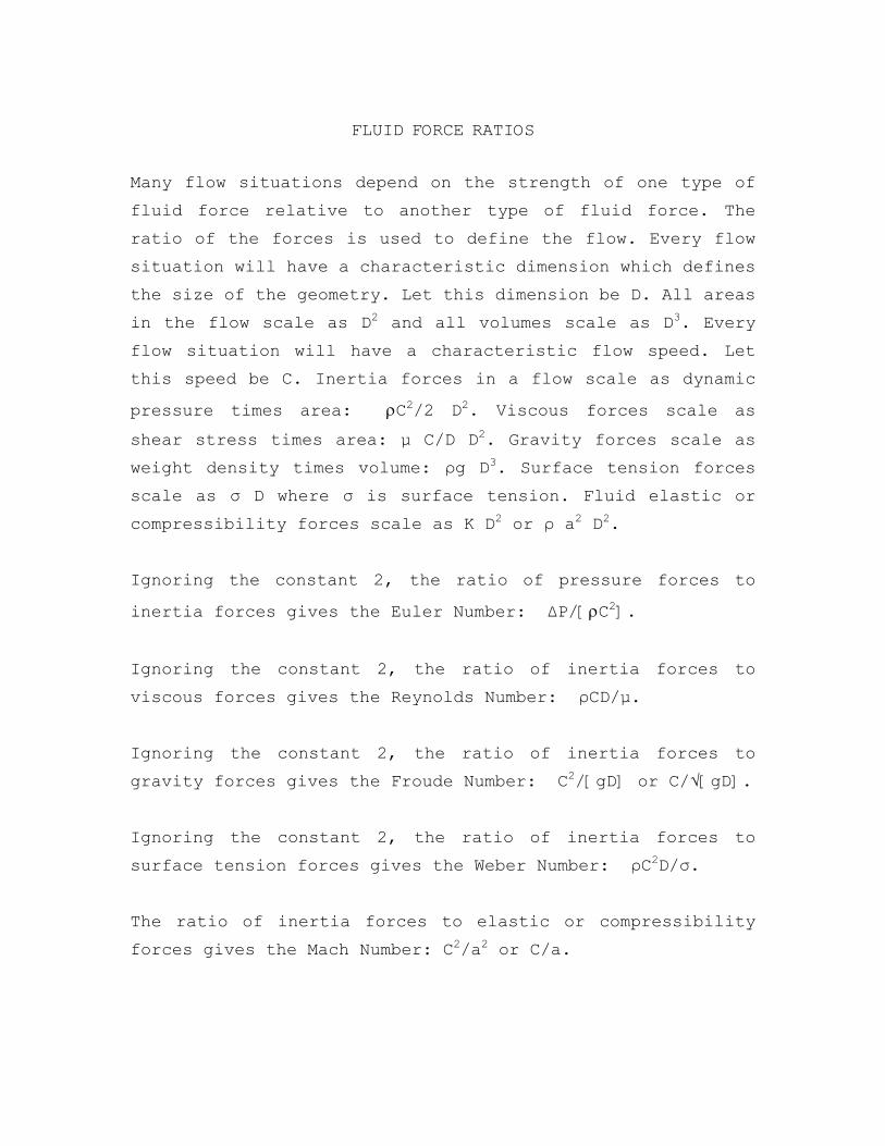
FLUID FORCE RATIOS
Many flow situations depend on the strength of one type of
fluid force relative to another type of fluid force. The
ratio of the forces is used to define the flow. Every flow
situation will have a characteristic dimension which defines
the size of the geometry. Let this dimension be D. All areas
in the flow scale as D2 and all volumes scale as D3. Every
flow situation will have a characteristic flow speed. Let
this speed be C. Inertia forces in a flow scale as dynamic
pressure times area: C2/2 D2. Viscous forces scale as
shear stress times area: µ C/D D2. Gravity forces scale as
weight density times volume: ρg D3. Surface tension forces
scale as σ D where σ is surface tension. Fluid elastic or
compressibility forces scale as K D2 or ρ a2 D2.
Ignoring the constant 2, the ratio of pressure forces to
inertia forces gives the Euler Number: ΔP/[C2].
Ignoring the constant 2, the ratio of inertia forces to
viscous forces gives the Reynolds Number: ρCD/µ.
Ignoring the constant 2, the ratio of inertia forces to
gravity forces gives the Froude Number: C2/[gD] or C/√[gD].
Ignoring the constant 2, the ratio of inertia forces to
surface tension forces gives the Weber Number: ρC2D/σ.
The ratio of inertia forces to elastic or compressibility
forces gives the Mach Number: C2/a2 or C/a.
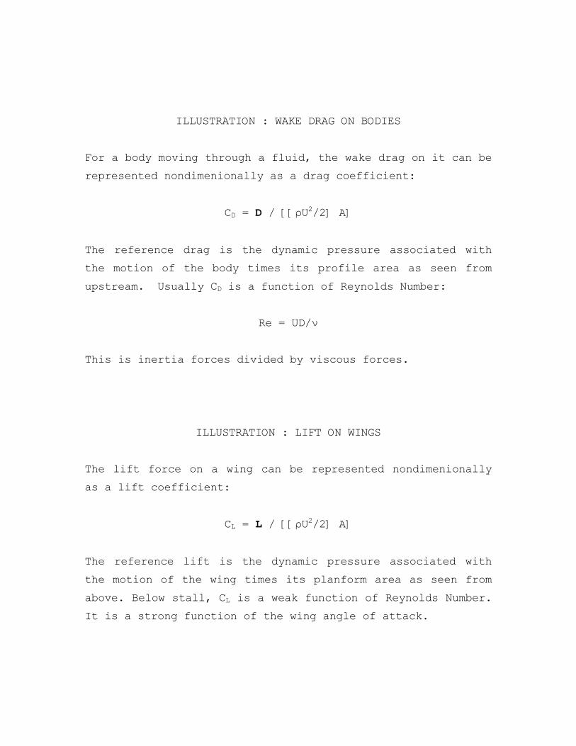
ILLUSTRATION : WAKE DRAG ON BODIES
For a body moving through a fluid, the wake drag on it can be
represented nondimenionally as a drag coefficient:
CD = D / [[ρU2/2] A]
The reference drag is the dynamic pressure associated with
the motion of the body times its profile area as seen from
upstream. Usually CD is a function of Reynolds Number:
Re = UD/ν
This is inertia forces divided by viscous forces.
ILLUSTRATION : LIFT ON WINGS
The lift force on a wing can be represented nondimenionally
as a lift coefficient:
CL = L / [[ρU2/2] A]
The reference lift is the dynamic pressure associated with
the motion of the wing times its planform area as seen from
above. Below stall, CL is a weak function of Reynolds Number.
It is a strong function of the wing angle of attack.
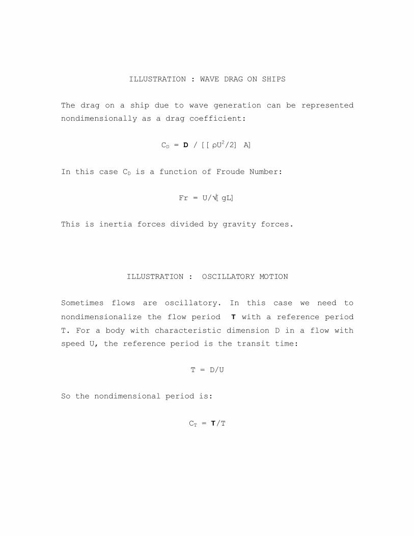
ILLUSTRATION : WAVE DRAG ON SHIPS
The drag on a ship due to wave generation can be represented
nondimensionally as a drag coefficient:
CD = D / [[ρU2/2] A]
In this case CD is a function of Froude Number:
Fr = U/√[gL]
This is inertia forces divided by gravity forces.
ILLUSTRATION : OSCILLATORY MOTION
Sometimes flows are oscillatory. In this case we need to
nondimensionalize the flow period T with a reference period
T. For a body with characteristic dimension D in a flow with
speed U, the reference period is the transit time:
T = D/U
So the nondimensional period is:
CT = T/T
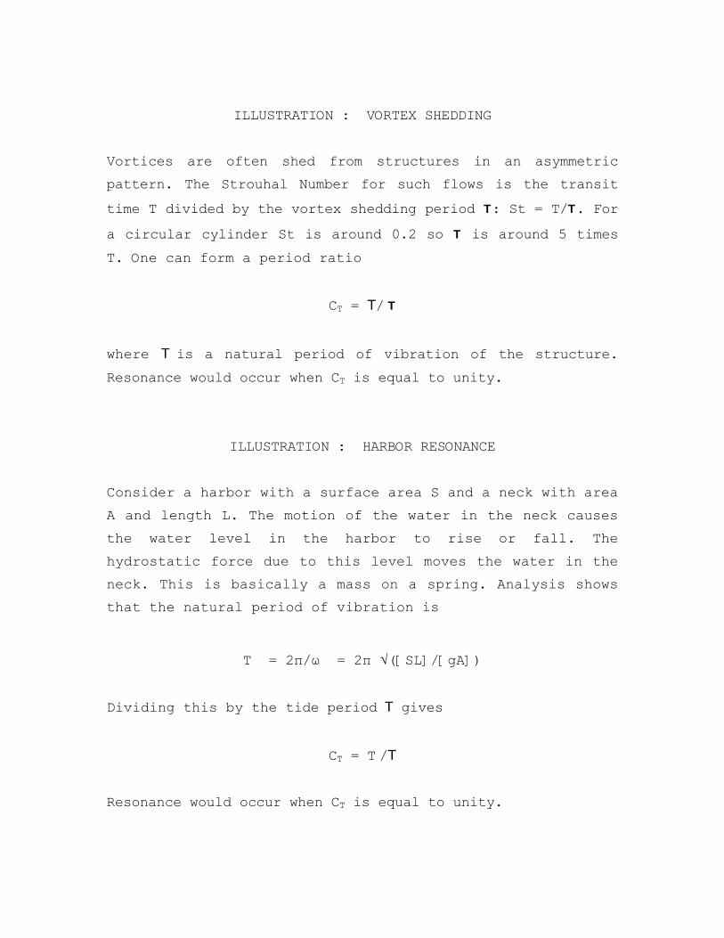
ILLUSTRATION : VORTEX SHEDDING
Vortices are often shed from structures in an asymmetric
pattern. The Strouhal Number for such flows is the transit
time T divided by the vortex shedding period T: St = T/T. For
a circular cylinder St is around 0.2 so T is around 5 times
T. One can form a period ratio
CT = T/ T
where T is a natural period of vibration of the structure.
Resonance would occur when CT is equal to unity.
ILLUSTRATION : HARBOR RESONANCE
Consider a harbor with a surface area S and a neck with area
A and length L. The motion of the water in the neck causes
the water level in the harbor to rise or fall. The
hydrostatic force due to this level moves the water in the
neck. This is basically a mass on a spring. Analysis shows
that the natural period of vibration is
T = 2π/ω = 2π √([SL]/[gA])
Dividing this by the tide period T gives
CT = T /T
Resonance would occur when CT is equal to unity.
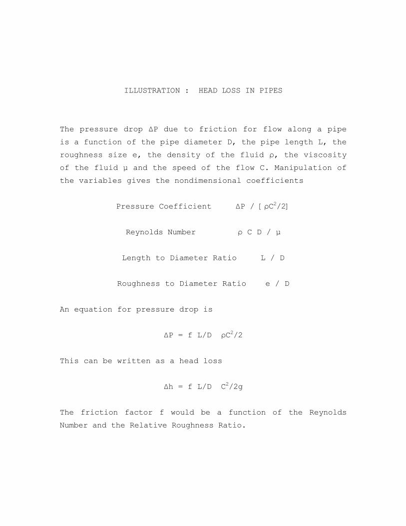
ILLUSTRATION : HEAD LOSS IN PIPES
The pressure drop ΔP due to friction for flow along a pipe
is a function of the pipe diameter D, the pipe length L, the
roughness size e, the density of the fluid ρ, the viscosity
of the fluid µ and the speed of the flow C. Manipulation of
the variables gives the nondimensional coefficients
Pressure Coefficient ΔP / [ρC2/2]
Reynolds Number ρ C D / µ
Length to Diameter Ratio L / D
Roughness to Diameter Ratio e / D
An equation for pressure drop is
ΔP = f L/D ρC2/2
This can be written as a head loss
Δh = f L/D C2/2g
The friction factor f would be a function of the Reynolds
Number and the Relative Roughness Ratio.
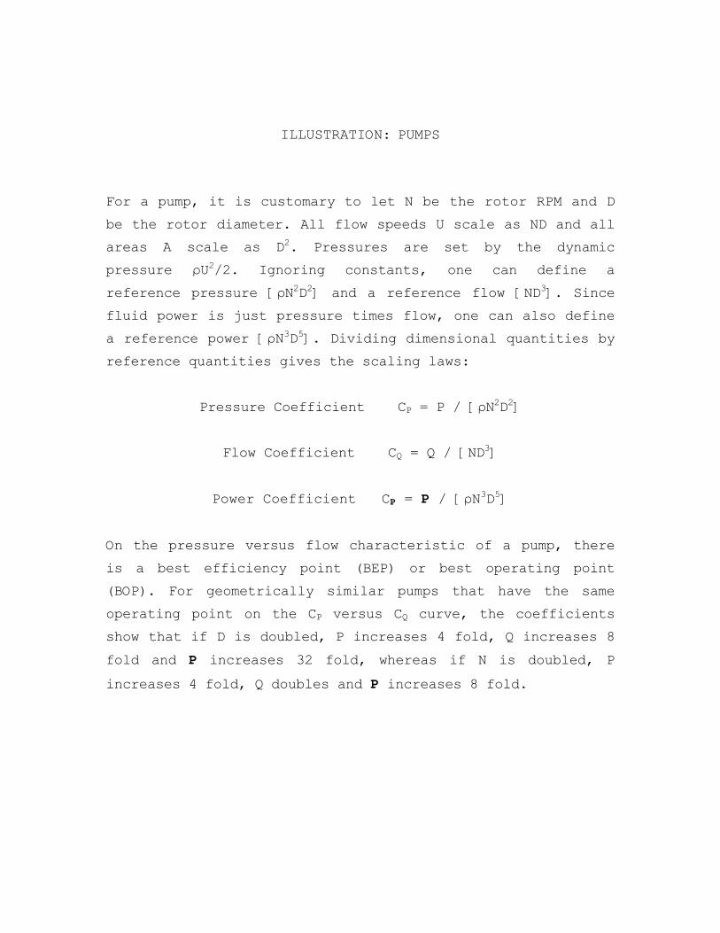
ILLUSTRATION: PUMPS
For a pump, it is customary to let N be the rotor RPM and D
be the rotor diameter. All flow speeds U scale as ND and all
areas A scale as D2. Pressures are set by the dynamic
pressure ρU2/2. Ignoring constants, one can define a
reference pressure [ρN2D2] and a reference flow [ND3]. Since
fluid power is just pressure times flow, one can also define
a reference power [ρN3D5]. Dividing dimensional quantities by
reference quantities gives the scaling laws:
Pressure Coefficient CP = P / [ρN2D2]
Flow Coefficient CQ = Q / [ND3]
Power Coefficient CP = P / [ρN3D5]
On the pressure versus flow characteristic of a pump, there
is a best efficiency point (BEP) or best operating point
(BOP). For geometrically similar pumps that have the same
operating point on the CP versus CQ curve, the coefficients
show that if D is doubled, P increases 4 fold, Q increases 8
fold and P increases 32 fold, whereas if N is doubled, P
increases 4 fold, Q doubles and P increases 8 fold.
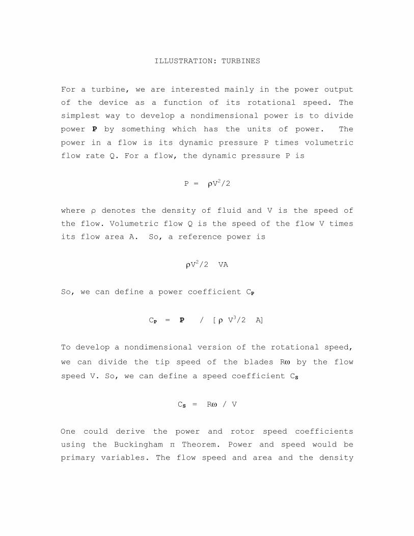
ILLUSTRATION: TURBINES
For a turbine, we are interested mainly in the power output
of the device as a function of its rotational speed. The
simplest way to develop a nondimensional power is to divide
power P by something which has the units of power. The
power in a flow is its dynamic pressure P times volumetric
flow rate Q. For a flow, the dynamic pressure P is
P = V2/2
where ρ denotes the density of fluid and V is the speed of
the flow. Volumetric flow Q is the speed of the flow V times
its flow area A. So, a reference power is
V2/2 VA
So, we can define a power coefficient CP
CP = P / [ V3/2 A]
To develop a nondimensional version of the rotational speed,
we can divide the tip speed of the blades R by the flow
speed V. So, we can define a speed coefficient CS
CS = R / V
One could derive the power and rotor speed coefficients
using the Buckingham π Theorem. Power and speed would be
primary variables. The flow speed and area and the density
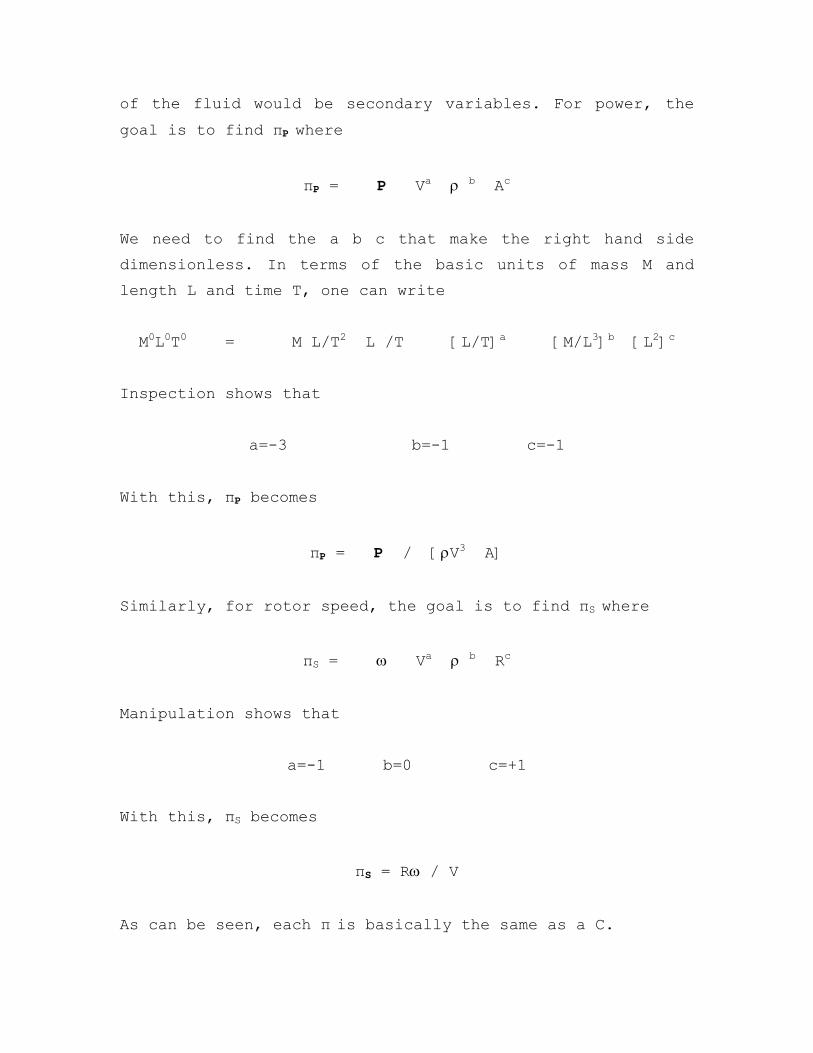
of the fluid would be secondary variables. For power, the
goal is to find πP where
πP = P Va b Ac
We need to find the a b c that make the right hand side
dimensionless. In terms of the basic units of mass M and
length L and time T, one can write
M0L0T0 = M L/T2 L /T [L/T]a [M/L3]b [L2]c
Inspection shows that
a=-3 b=-1 c=-1
With this, πP becomes
πP = P / [V3 A]
Similarly, for rotor speed, the goal is to find πS where
πS = Va b Rc
Manipulation shows that
a=-1 b=0 c=+1
With this, πS becomes
πS = R / V
As can be seen, each π is basically the same as a C.


![L-14 Fluids [3] Fluids at rest Fluids at rest Why things float Archimedes’ Principle Fluids in Motion Fluid Dynamics Fluids in Motion Fluid Dynamics.](https://static.fdocuments.in/doc/165x107/56649d845503460f94a6ab30/l-14-fluids-3-fluids-at-rest-fluids-at-rest-why-things-float-archimedes.jpg)
![L-14 Fluids [3] Fluids at rest Why things float Archimedes’ Principle Fluids in Motion Fluid Dynamics –Hydrodynamics –Aerodynamics.](https://static.fdocuments.in/doc/165x107/56649d9f5503460f94a89e67/l-14-fluids-3-fluids-at-rest-why-things-float-archimedes-principle.jpg)


![L-14 Fluids [3] Fluids at rest Fluid Statics Fluids at rest Fluid Statics Why things float Archimedes’ Principle Fluids in Motion Fluid Dynamics.](https://static.fdocuments.in/doc/165x107/56649ced5503460f949ba1d5/l-14-fluids-3-fluids-at-rest-fluid-statics-fluids-at-rest-fluid-statics.jpg)