
Fluidfoil Impellers A3 as aftp.feq.ufu.br/Luis_Claudio/Books/E-Books/Engineering... · ·...
13
Agitation I91 3.1 Fluidfoil Impellers The introduction of fluidfoil impellers, as shown in Fig. 9a through 9f, give a wide variety of mixing conditions suitable for high flow and low fluid shear rates. Fluidfoil impellers use the principles developed in airfoil work in wind tunnels for aircraft. Figure 10a shows what is desirable, which is no form separation of the fluid, and maximum lift and drag coefficients, which is what one is trying to achieve with the fluidfoil impellers. Figure 10b shows what happens when the angle and the shape is such that there is a separation ofthe fluid from the airfoil body. The A3 10 impeller (Fig. Sa) was introduced for primarily low viscosity fluids and, as can be seen, has a very low ratio of total blade surface area compared to an inscribing circle which is shown in Fig. 11. When the fluid viscosities are higher, the A3 12 impeller is used (shown in Fig. 9b) which is particularly useful in fibrous materials. To give a more responsive action in higher viscosities, the A320 is available which works well in the transition area of Reynolds numbers. When gas-liquid processes are used, the A3 15 (Figure 9d) has a still higher solidity ratio. It is particularly useful in aerobic fermentation processes. Impellers in Figs. 9(a-d) are formed from flat metal stock. To complete the current picture, when composite materials are used, the airfoil can be shaped in any way that is desirable. The A6000 (Fig. 9e) illustrates that particular impeller type. The use of proplets on the end of the blades increases flow about 10% over not having them. An impeller which is able to operate effectively in both the turbulent and transitional Reynolds numbers is the A4 10 (Fig. 9 0 which has a very marked increase in twist angle ofthe blade. This gives it a more effective performance in the higher viscosity fluids encountered in mixers up to about 3 kW. One characteristic of these fluidfoil impellers is that they discharge a stream that is almost completely axial flow and they have a very uniform velocity across the discharge plane of the impeller. However, there is a tendency for these impellers to short-circuit the fluid to a relatively low distance above the impeller. Very careful consideration of the coverage over the impeller is important. If the impeller can be placed one to two impeller diameters off bottom, which means that mixing is not provided at low levels during draw off, these impellers offer an excellent flow pattern as well as considerable economies in shaft design. To look at these impellers in a different way, three impellers have been compared at equal total-pumping capacity. Figure 12 gives the output velocity as a function of time on a strip chart. As can be seen in Fig. 12 the fluidfoil impeller type (A3 10) has a very low velocity fluctuation and uses
Transcript of Fluidfoil Impellers A3 as aftp.feq.ufu.br/Luis_Claudio/Books/E-Books/Engineering... · ·...

Agitation I91
3.1 Fluidfoil Impellers
The introduction of fluidfoil impellers, as shown in Fig. 9a through 9f, give a wide variety of mixing conditions suitable for high flow and low fluid shear rates. Fluidfoil impellers use the principles developed in airfoil work in wind tunnels for aircraft. Figure 10a shows what is desirable, which is no form separation of the fluid, and maximum lift and drag coefficients, which is what one is trying to achieve with the fluidfoil impellers. Figure 10b shows what happens when the angle and the shape is such that there is a separation ofthe fluid from the airfoil body. The A3 10 impeller (Fig. Sa) was introduced for primarily low viscosity fluids and, as can be seen, has a very low ratio of total blade surface area compared to an inscribing circle which is shown in Fig. 11. When the fluid viscosities are higher, the A3 12 impeller is used (shown in Fig. 9b) which is particularly useful in fibrous materials.
To give a more responsive action in higher viscosities, the A320 is available which works well in the transition area of Reynolds numbers. When gas-liquid processes are used, the A3 15 (Figure 9d) has a still higher solidity ratio. It is particularly useful in aerobic fermentation processes. Impellers in Figs. 9(a-d) are formed from flat metal stock.
To complete the current picture, when composite materials are used, the airfoil can be shaped in any way that is desirable. The A6000 (Fig. 9e) illustrates that particular impeller type. The use of proplets on the end of the blades increases flow about 10% over not having them. An impeller which is able to operate effectively in both the turbulent and transitional Reynolds numbers is the A4 10 (Fig. 9 0 which has a very marked increase in twist angle ofthe blade. This gives it a more effective performance in the higher viscosity fluids encountered in mixers up to about 3 kW.
One characteristic of these fluidfoil impellers is that they discharge a stream that is almost completely axial flow and they have a very uniform velocity across the discharge plane of the impeller. However, there is a tendency for these impellers to short-circuit the fluid to a relatively low distance above the impeller. Very careful consideration of the coverage over the impeller is important. If the impeller can be placed one to two impeller diameters off bottom, which means that mixing is not provided at low levels during draw off, these impellers offer an excellent flow pattern as well as considerable economies in shaft design.
To look at these impellers in a different way, three impellers have been compared at equal total-pumping capacity. Figure 12 gives the output velocity as a function of time on a strip chart. As can be seen in Fig. 12 the fluidfoil impeller type (A3 10) has a very low velocity fluctuation and uses

Fermentation and Biochemical Engineering Handbook192
much less power than the other two impellers. For the same flow, the A200impeller has a higher turbulent fluctuation value. The Rl 00 impeller has stillhigher power consumption at the same diameter than the other two impellers,and has a much more intense level of microscale turbulence.
The fluidfoil impellers are often called "high efficiency impellers", butthat is true only in terms offlow, and makes the assumption that flow is themain measure of mixing results. Flow is one measure, and in at least half ofthe mixing applications is a good measure of the performance that could beexpected in a process. These impellers are low in efficiency in providing shearrates-either of the macro scale or the micro scale.
The use of computer generated solutions to problems and computa-tional fluid dynamics is also another approach of comparing impellers andprocess results. There are software packages available. It is very helpful tohave data obtained from a laser velocity meter on the fluid mechanics of theimpeller flow and other characteristics to put in the boundary conditions forthese computer programs.
Figure 9a. A310 fluidfoil impeller.

Agitation 193
Figure 9b. A312 Fluidfoil impeller.
Figure 9c. A320 fluidfoil impeller.

Fermentation and Biochemical Engineering Handbook194
Figure 9d. A315 fluidfoil impeller
Figure ge. A6000 fluidfoil impeller made of composite materials
Agitation 195
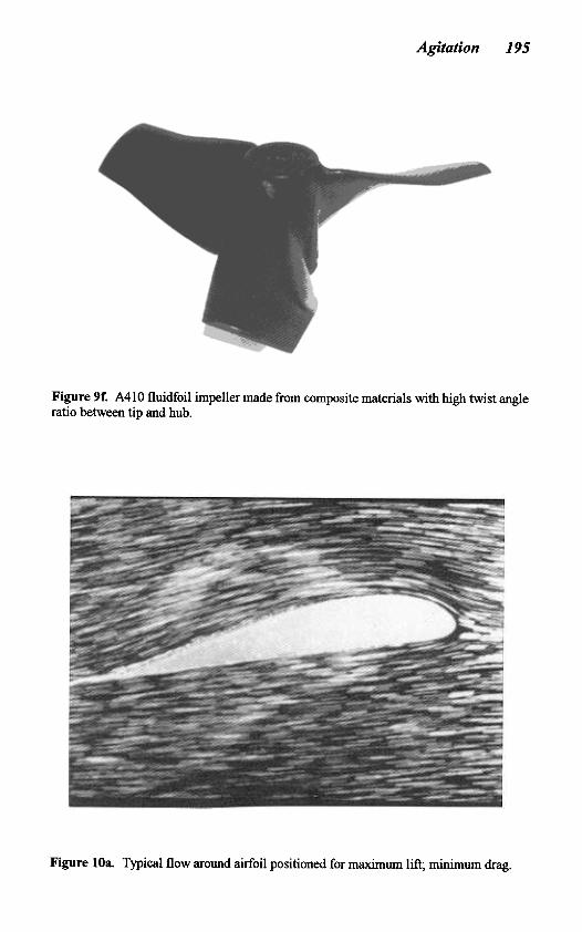
Figure 9(. A410 fluidfoil impeller made from composite materials with high twist angleratio between tip and hub.
Figure lOa. Typical flow around airfoil positioned for maximwn lift; minimwn drag.
Fermentation and Biochemical Engineering Handbook196
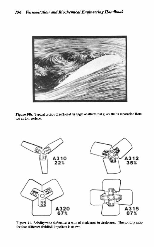
Figure lOb. Typical profile of airfoil at an angle of attack that gives fluids separation from
the airfoil surface.
Figure 11. Solidity ratio defmed as a ratio of blade area to circle area. The solidity ratiofor four different fluidfoil impellers is shown.

Agitation I9 7
4 -
3 -
OUTLET VELOCITY v s TIME
1 4 . 4
l 3 I
3 ’
S
Figure 12. Velocity trace with time for three different impeller types, A3 10 fluidfoil, A200 axial flow turbine and RlOO radial flow turbine. The impellers are compared at equal discharge pumping capacity, equal diameter and at whatever speed is required to achieve this flow. The power required increases from left to right.
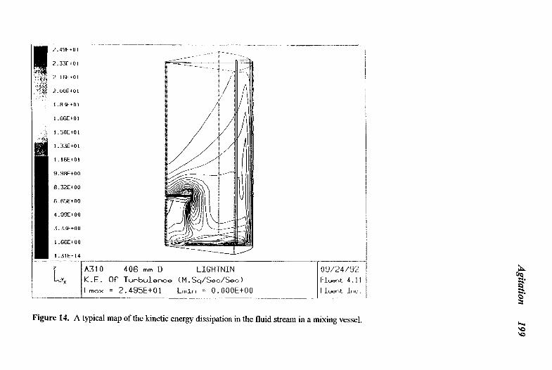
As an example of other types of programs that can be worked on, Fig. 13 shows a velocity profile from an A410 impeller, Fig. 14, a map of the kinetic energy dissipation in the fluid stream and in the third one (Fig. 15) model of heavier than the liquid particles in a random tracking pattern.
Additional models can be made up using mass transfer, heat transfer and some reaction kinetics to simulate aprocess that can be defined in one or more of those types of relationships.
The laser velocity meter has made it possible to obtain much data from experiments conducted in transparent fluids. Figure 16 shows a typical output of such a measurement, giving lines that are proportioned to the fluid at that point and also relate to that angle of discharge. Studies on the blending and process performance of these various fluidfoil impellers will be covered in later sections of this chapter.

198 F
ermentation and B
iochemical E
ngineering Handbook 0
0
+
LiJ z
o
HO
z-0
I-
-0
'
I mo
ur
n
H \
II
L
v
0
(0
0
LO
E
O+
E
JJ
W
u+
co
mo
, o
>m
Agitation
I99
.
0
0
-4
.
ow
z
oo
H
Cn
O
z\o
co
I a
0
um
H
\
$1 -Io-
mc
c
0
I1

200 F
ermentation and B
iochemical E
ngineering Handbook

Agitation 201
LlGHTNlN A 3 10
Figure 16. Typical laser output from the measurement of velocities by means of a Doppler velocity meter.
4.0 BAFFLES
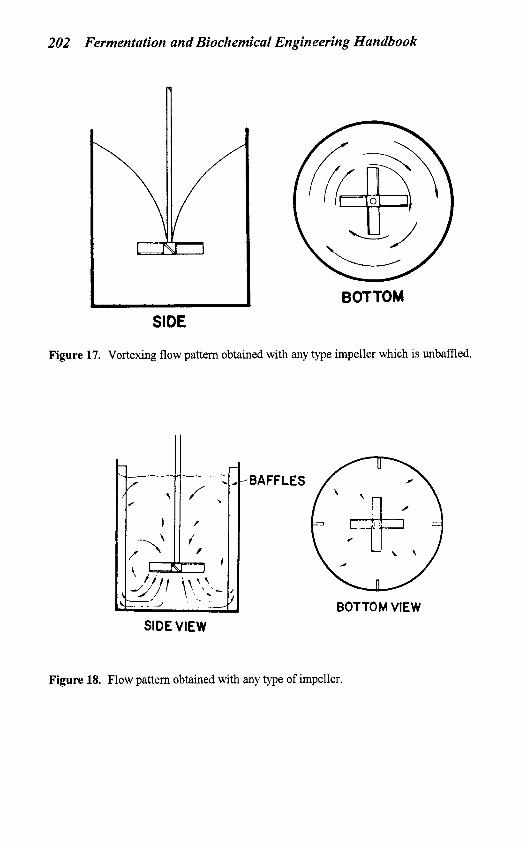
Figure 17 illustrates the flow pattern in an unbaffled tank. The swirl and vortex are normally undesirable. Putting four baffles in the tank, as shown in Fig. 18, allows the application of any amount of horsepower to the system without the tendency to swirl and vortex. Either 3 , 6 or 8 baffles can be used if preferred. The general principle is to use the same total projected area as exists with four baffles, each 1/12 the tank diameter in width. For square or rectangular tanks the baffles shown in Fig. 19 are typical. At power levels below 1 hp/1000 gal., the corners in square or rectangular tanks often give sufficient baffling that additional wall baffles are not needed.
202 Fermentation and Biochemical Engineering Handbook
BOTTOM SIDE
Figure 17. Vortexing flow pattern obtained with any type impeller which is unbafled.
SIDE VIEW
-BAFFLES
BOTTOM VIEW
Figure 18. Flow pattern obtained with any type of impeller.

Agitation 203
I I -.&.- I
W
1. k IF NEEDED
L-1.5WS L= 2w -4 Figure 19. Suggested bafles for square and rectangular tanks.
5.0 FLUID SHEAR RATES
Figure 20 illustrates flow pattern in the laminar flow region from a radial flat blade turbine. By using a velocity probe, the parabolic velocity distribution coming off the blades of the impeller is shown in Fig. 2 1. By taking the slope of the curve at any point, the shear rate may be calculated at that point. The maximum shear rate around the impeller periphery as well as the average shear rate around the impeller may also be calculated.
An important concept is that one must multiply the fluid shear rate from the impeller by the viscosity of the fluid to get the fluid shear stress that actually carries out the process of mixing and dispersion.
Fluid shear stress = p(fluid shear rate)
Even in low viscosity fluids, by going from 1 cp to 10 cp there will be 10 times the shear stress of the process operating from the fluid shear rate of the impeller.