FLUID STATICS No flow Surfaces of const P and coincide along gravitational equipotential surfaces h...
105
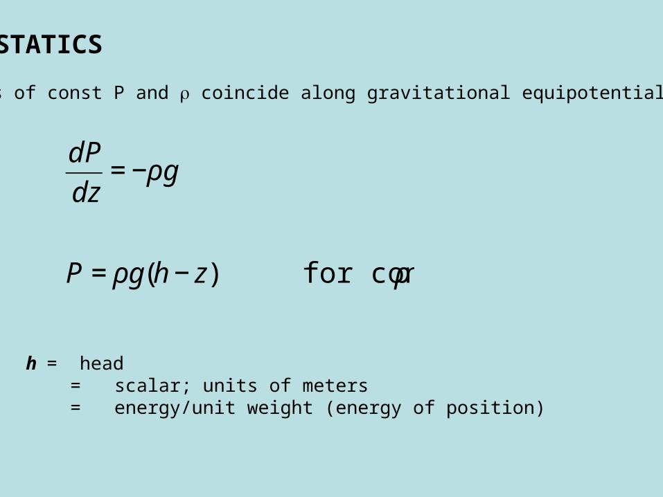
STATICS s of const P and coincide along gravitational equipotential dP dz =− ρg P = ρg ( h − z ) for con ρ h = head = scalar; units of meters = energy/unit weight (energy of position)
-
Upload
sabrina-heath -
Category
Documents
-
view
218 -
download
2
Transcript of FLUID STATICS No flow Surfaces of const P and coincide along gravitational equipotential surfaces h...
FLUID STATICS No flowSurfaces of const P and coincide along gravitational equipotential surfaces
€
dP
dz= −ρg
P = ρg(h − z) for constant ρ
h = head = scalar; units of meters = energy/unit weight (energy of position)
P = 1 atm surface
P ~ 1.3 atm @10 feet
P ~ 1.6 atm @20 feet
P ~ 2 atm @33 feet
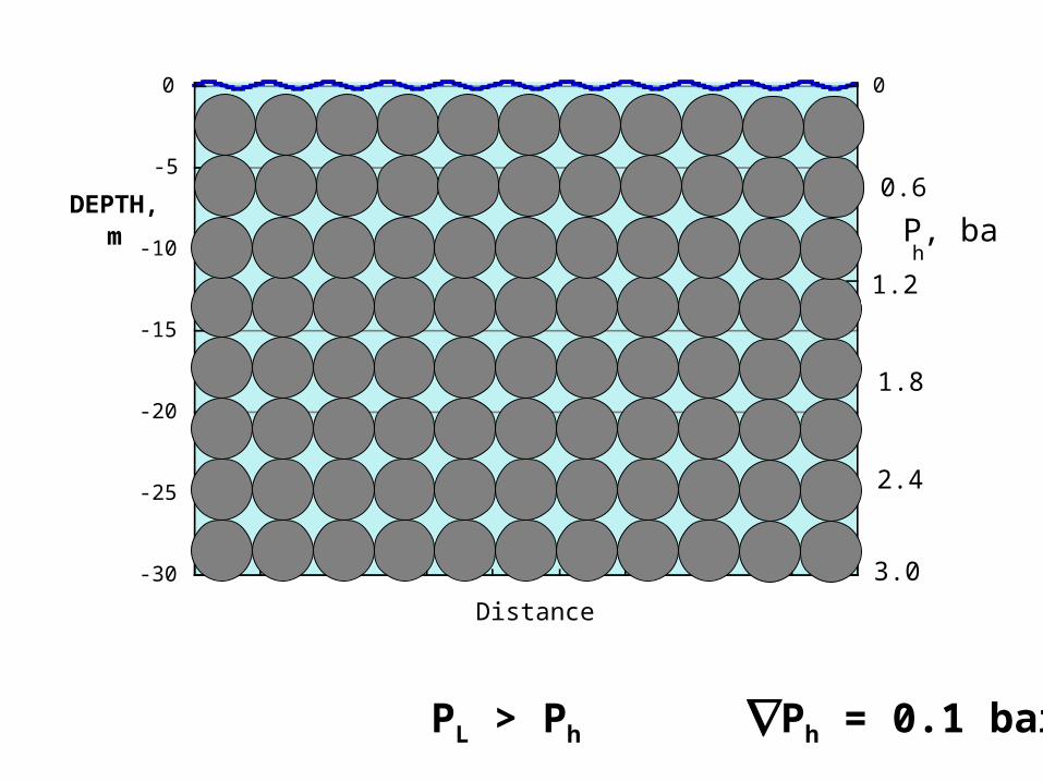
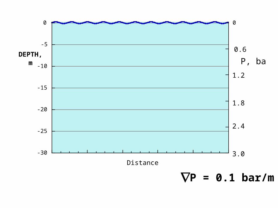
P 0.1 bar/m

-30
-25
-20
-15
-10
-5
0 0
0.2
0.4
0.6
0.8
1
DEPTH, m
Distance
P, bar
P = 0.1 bar/m
0.6
1.2
2.4
1.8
3.0
-30
-25
-20
-15
-10
-5
0 0
0.2
0.4
0.6
0.8
1
DEPTH, m
Distance
P, bar
-30
-25
-20
-15
-10
-5
0 0
0.2
0.4
0.6
0.8
1
DEPTH, m
Distance
P, barh
PL > Ph Ph = 0.1 bar/m
0.6
1.2
1.8
2.4
3.0
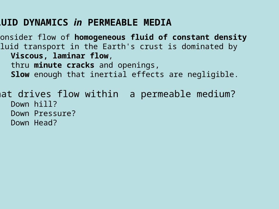
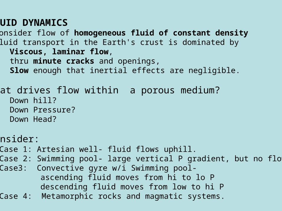
FLUID DYNAMICS in PERMEABLE MEDIA
Consider flow of homogeneous fluid of constant densityFluid transport in the Earth's crust is dominated by
Viscous, laminar flow, thru minute cracks and openings, Slow enough that inertial effects are negligible.
What drives flow within a permeable medium? Down hill?
Down Pressure? Down Head?
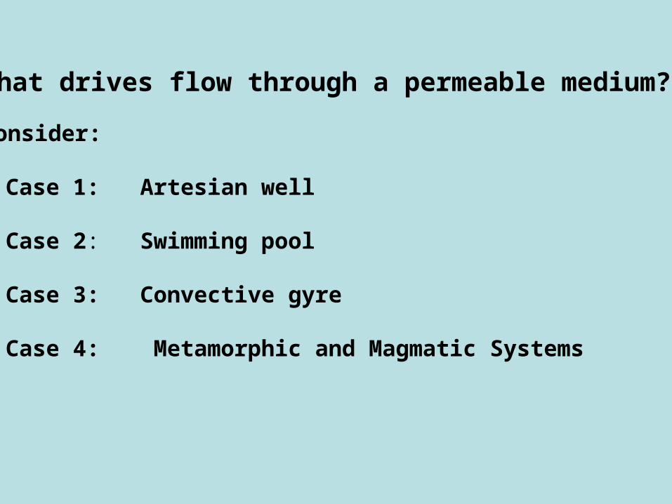
What drives flow through a permeable medium?
Consider:
Case 1: Artesian well
Case 2: Swimming pool
Case 3: Convective gyre
Case 4: Metamorphic and Magmatic Systems

Humble TexasFlowing 100 yearsHot, sulfur-rich, artesian water
http://www.texasescapes.com/TexasGulfCoastTowns/Humble-Texas.htm
-30
-25
-20
-15
-10
-5
0 0
0.2
0.4
0.6
0.8
1
DEPTH, m
Distance
P, bar
P = 0.1 bar/m
0.6
1.2
1.8
2.4
3.0

-30
-25
-20
-15
-10
-5
0 0
0.2
0.4
0.6
0.8
1
DEPTH, m
Distance
P, bar
P = 0.1bar/m
0.6
1.2
1.8
2.4
3.0
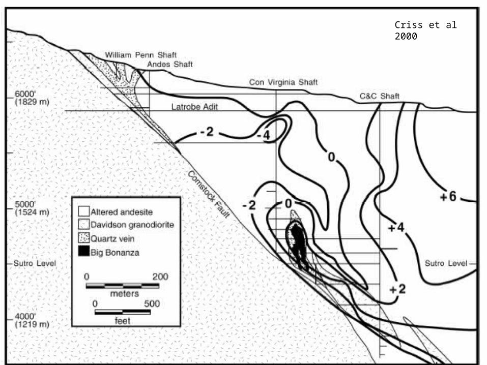
Criss et al 2000
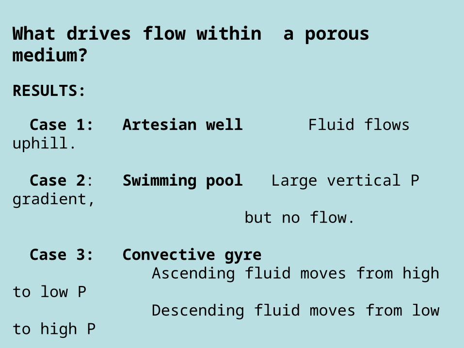
What drives flow within a porous medium?
RESULTS:
Case 1: Artesian well Fluid flows uphill.
Case 2: Swimming pool Large vertical P gradient,
but no flow.
Case 3: Convective gyre Ascending fluid moves from high to low P
Descending fluid moves from low to high P
Case 4: Metamorphic and Magmatic SystemsFluid flows both toward heat source, then
away,irrespective of pressure
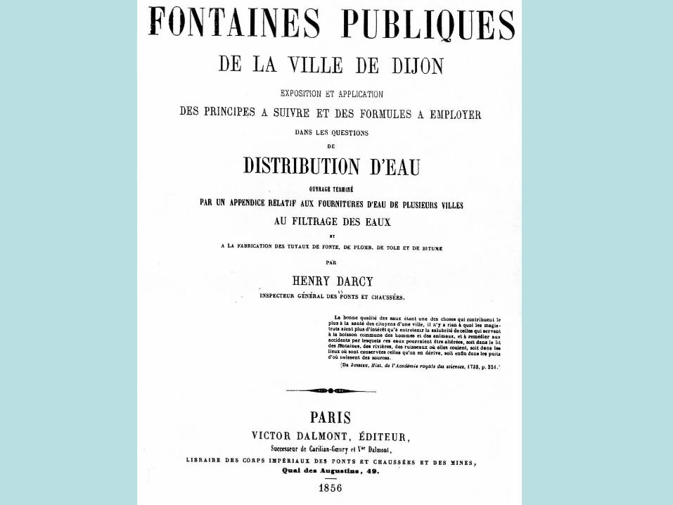

Darcy's Law Henry Darcy (1856) Sanitation Engineer
Public water supply for Dijon, France. Filtered water thru large sand column; attached Hg manometers
Observed relationship bt the volumetric flow rate and the hydraulic gradient
Q (hu -hl)/L
where (hu -hl) is the difference in upper & lower manometer readings L is the spacing length
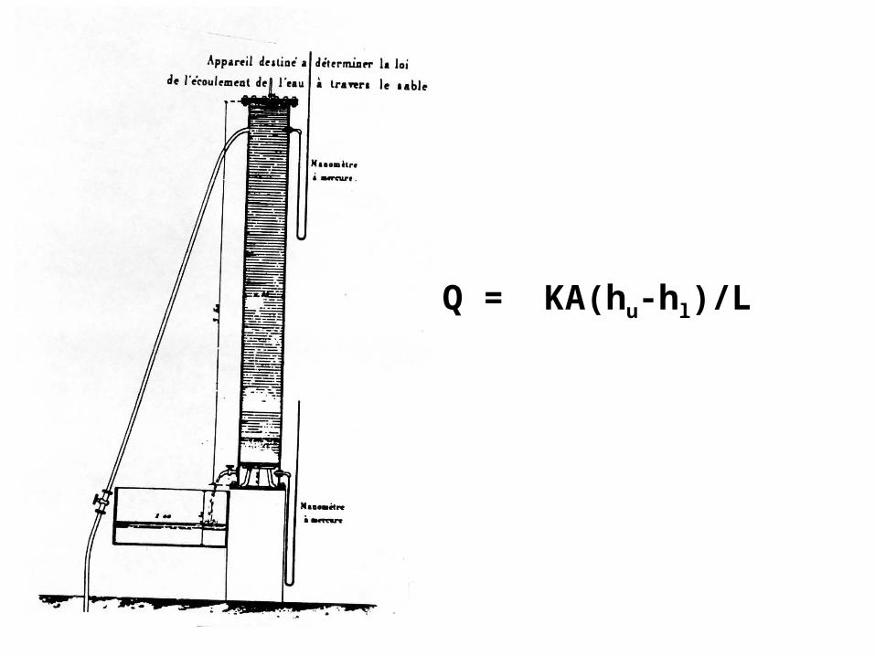
Q = KA(hu-hl)/L
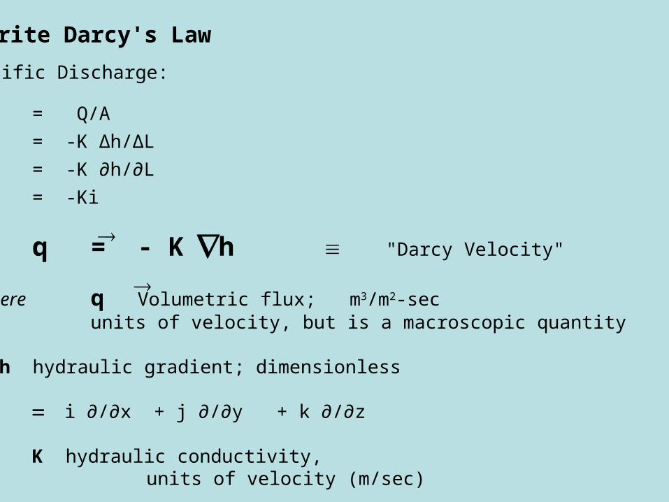
Rewrite Darcy's Law
Specific Discharge:
q = Q/A
= -K ∆h/∆L
= -K ∂h/∂L
= -Ki
q = - K h "Darcy Velocity" where q Volumetric flux; m3/m2-sec
units of velocity, but is a macroscopic quantity h hydraulic gradient; dimensionless
i ∂/∂x + j ∂/∂y + k ∂/∂z
K hydraulic conductivity, units of velocity (m/sec)
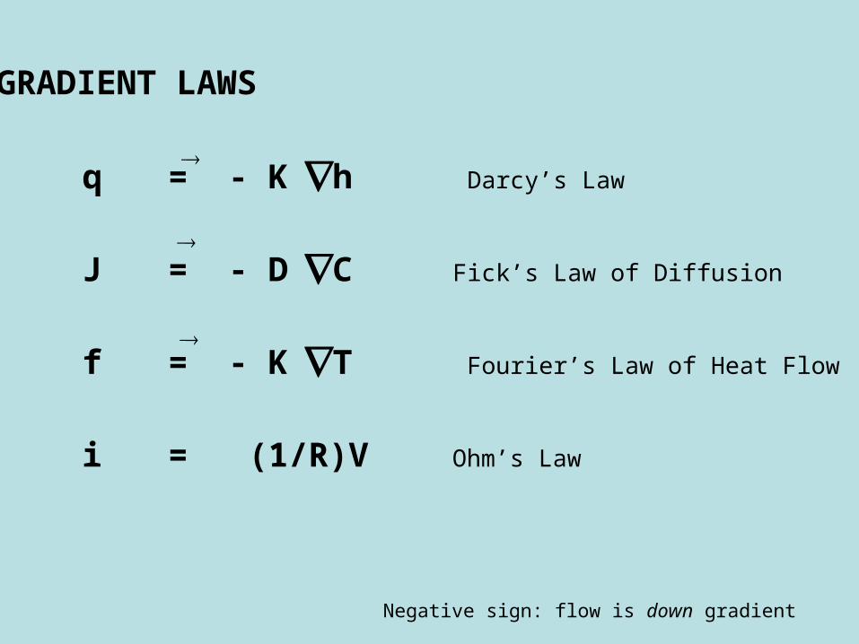
GRADIENT LAWS
q = - K h Darcy’s Law
J = - D C Fick’s Law of Diffusion
f = - K T Fourier’s Law of Heat Flow
i = (1/R)V Ohm’s Law
Negative sign: flow is down gradient
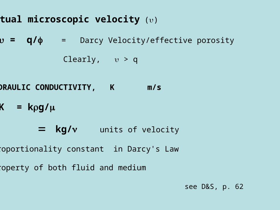
Actual microscopic velocity ()
= q/ = Darcy Velocity/effective porosity
Clearly, > q
HYDRAULIC CONDUCTIVITY, K m/s
K = kg/ kg/ units of velocity
Proportionality constant in Darcy's Law Property of both fluid and medium
see D&S, p. 62
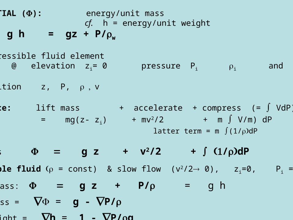
HYDRAULIC POTENTIAL (): energy/unit mass cf. h = energy/unit weight
= g h = gz + P/w
Consider incompressible fluid element @ elevation zi= 0 pressure Pi i and velocity v = 0
Move to new position z, P, v
Energy difference: lift mass + accelerate + compress (= VdP) = mg(z- zi) + mv2/2 + m V/m) dP
latter term = m (1/dP
Energy/unit mass g z + v2/2 + /dP
For incompressible fluid = const) & slow flow (v2/2 0), zi=0, Pi = 0
Energy/unit mass: g z + P/ = g h
Force/unit mass = = g - P/
Force/unit weight = h = 1 - P/g
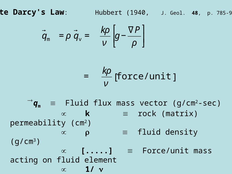
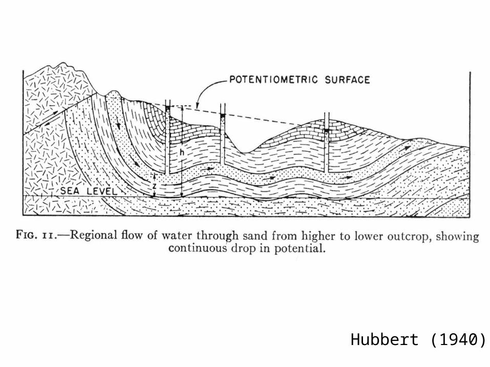
Rewrite Darcy's Law: Hubbert (1940, J. Geol. 48, p. 785-944)
qm Fluid flux mass vector (g/cm2-sec) k rock (matrix) permeability (cm2) fluid density (g/cm3) [.....] Force/unit mass acting on fluid
element 1/
where Kinematic Viscosity = cm2/sec
€
qm = ρ qv = kρ
νg −
∇P
ρ
⎡
⎣ ⎢
⎤
⎦ ⎥
= kρ
νforce/unit mass[ ]
€
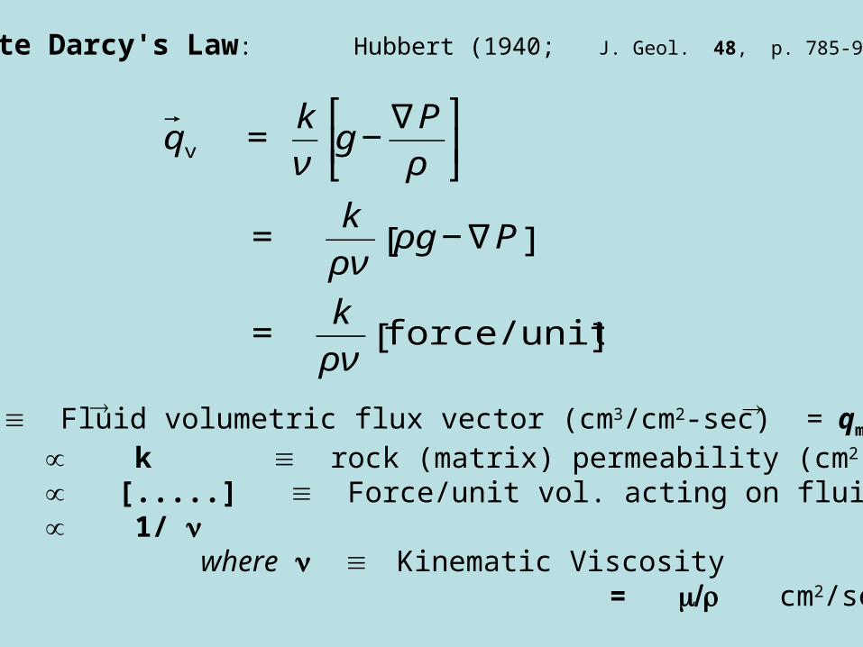
qv = k
νg −
∇P
ρ
⎡
⎣ ⎢
⎤
⎦ ⎥
= k
ρνρg − ∇P[ ]
= k
ρνforce/unit vol[ ]
Rewrite Darcy's Law: Hubbert (1940; J. Geol. 48, p. 785-944)
qv Fluid volumetric flux vector (cm3/cm2-sec) = qm
k rock (matrix) permeability (cm2) [.....] Force/unit vol. acting on fluid element 1/
where Kinematic Viscosity = cm2/sec
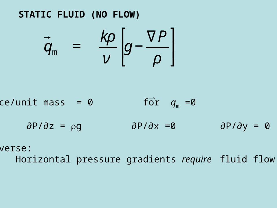
STATIC FLUID (NO FLOW)
€
qm = kρ
νg −
∇P
ρ
⎡
⎣ ⎢
⎤
⎦ ⎥
Force/unit mass = 0 for qm =0
∂P/∂z = g ∂P/∂x =0 ∂P/∂y = 0 Converse: Horizontal pressure gradients require fluid flow
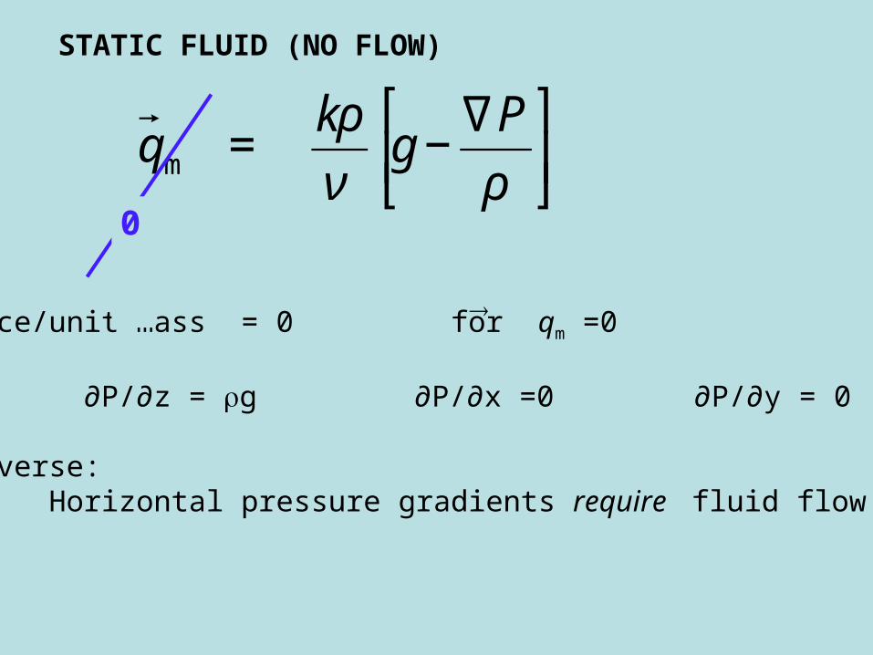
STATIC FLUID (NO FLOW)
€
qm = kρ
νg −
∇P
ρ
⎡
⎣ ⎢
⎤
⎦ ⎥
Force/unit mass = 0 for qm =0
∂P/∂z = g ∂P/∂x =0 ∂P/∂y = 0 Converse: Horizontal pressure gradients require fluid flow
0

Darcy's Law: Isotropic Media: q = - K h OK only if Kx = Ky = Kz
Darcy's Law: Anisotropic MediaK is a tensorSimplest case (orthorhombic?) where principal directions of anisotropy coincide with x, y, z
q = –
Kxx
0 0
0 Kyy
0
0 0 Kzz
i
∂ h
∂ x
j
∂ h
∂ y
k
∂ h
∂ z
q
x
= – Kxx
∂ h
∂ x
i qy
= – Kyy
∂ h
∂ y
j qz
= – Kzz
∂ h
∂ z
k
Thus
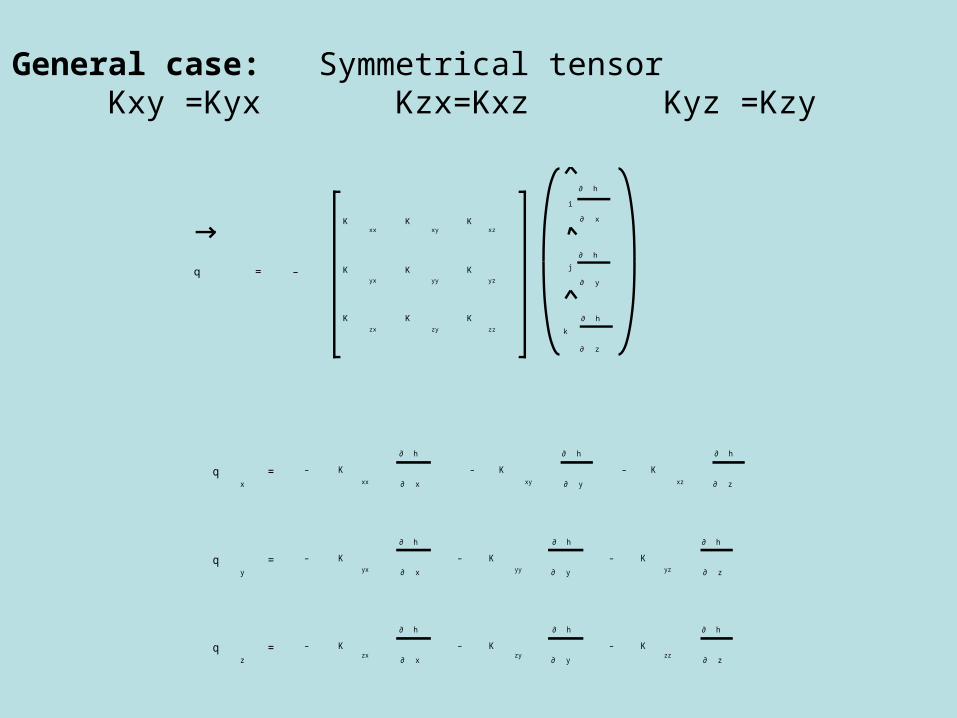
q = –
Kxx
Kxy
Kxz
Kyx
Kyy
Kyz
Kzx
Kzy
Kzz
i
∂ h
∂ x
j
∂ h
∂ y
k
∂ h
∂ z
General case: Symmetrical tensor Kxy =Kyx Kzx=Kxz Kyz =Kzy
q
x
= – Kxx
∂ h
∂ x
– Kxy
∂ h
∂ y
– Kxz
∂ h
∂ z
qy
= – Kyx
∂ h
∂ x
– Kyy
∂ h
∂ y
– Kyz
∂ h
∂ z
qz
= – Kzx
∂ h
∂ x
– Kzy
∂ h
∂ y
– Kzz
∂ h
∂ z

End
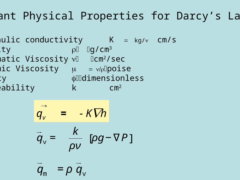
Relevant Physical Properties for Darcy’s Law
Hydraulic conductivity K kg/ cm/sDensity g/cm3
Kinematic Viscosity cm2/secDynamic Viscosity poise
Porosity dimensionlessPermeability k cm2
€
qv = k
ρν ρg − ∇P[ ]
€
qm = ρ qv
qv = - Kh

DENSITY () g/cm3
also, Specific weight (weight density) g
= f(T,P)
α ≡
V
∂ V
∂ TP
= –
∂
∂ TP
because
d
= –
dV
V
Thermal expansivity
βT
≡ –
1
V
∂ V
∂ PT
=
1
ρ
∂ ρ
∂ PT
Isothermal Compressibility
ρ
T , P
≅ ρo
1 – α ( T – To
) + β ( P – Po
)
for small α , β
where
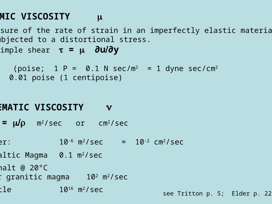
DYNAMIC VISCOSITY A measure of the rate of strain in an imperfectly elastic material
subjected to a distortional stress. For simple shear = ∂u∂y
Units (poise; 1 P = 0.1 N sec/m2 = 1 dyne sec/cm2
Water 0.01 poise (1 centipoise)
KINEMATIC VISCOSITY = m2/sec or cm2/sec
Water: 10-6 m2/sec = 10-2 cm2/sec
Basaltic Magma 0.1 m2/sec
Asphalt @ 20°C or granitic magma 102 m2/sec
Mantle 1016 m2/sec see Tritton p. 5; Elder p. 221)

Darcy's Law: Hubbert (1940; J. Geol. 48, p. 785-944)
where:
qv Darcy Velocity, Specific Discharge or Fluid volumetric flux vector (cm/sec)
k permeability (cm2)
K = kg/ hydraulic conductivity (cm/sec)
Kinematic viscosity, cm2/sec
€
qv = k
νg −
∇P
ρ
⎡
⎣ ⎢
⎤
⎦ ⎥ = -
kg
ν∇h[ ] = − K∇h

POROSITY ( or n) dimensionless
Ratio of void space to total volume of material
= Vv/VT
Dictates how much water a saturated material can contain
Important influence on bulk properties of material e.g., bulk , heat cap., seismic velocity……
Difference between Darcy velocity and average microscopic velocity
Decrease with depth: Shales = oe-cz exponential
Sandstones: = o - c z linear
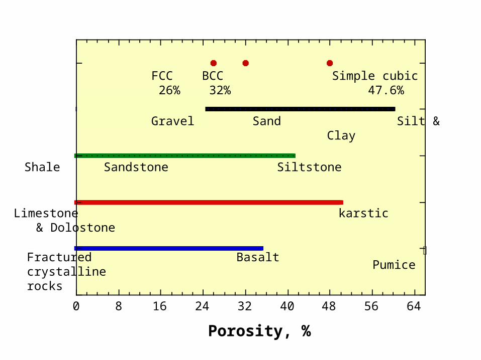
0 8 16 24 32 40 48 56 64
Porosity, %
Fractured Basaltcrystallinerocks
Limestone karstic & Dolostone
Shale Sandstone Siltstone
Gravel Sand Silt & Clay
FCC BCC Simple cubic 26% 32% 47.6%
Pumice
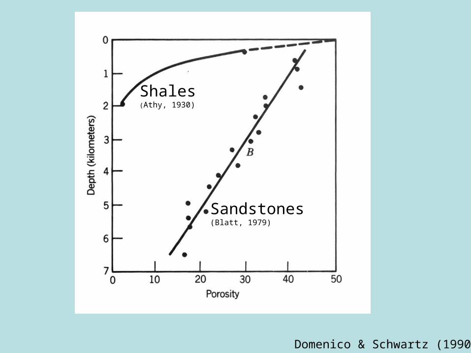
Domenico & Schwartz (1990)
Shales (Athy, 1930)
Sandstones (Blatt, 1979)

PERMEABILITY (k) units cm2
Measure of the ability of a material to transmit fluid under a hydrostatic gradient
Most important rock parameter pertinent to fluid flow
Relates to the presence of fractures and interconnected voids
1 darcy 0.987 x 10⁻⁸ cm2 .987 x 10-12 m2 (e.g., sandstone)
Approximate relation between K and k Km/s 107 k m
2 10-5 kdarcy

2
10 10 10 10 10 10 10 10 10-18 -16 -14 -12 -10 -8 -6 -4 -2
PERMEABILITY, cm
1nd 1d 1 md 1 d 1000d
Clay Silt Sand Gravel
Shale Sandstone
argillaceous Limestone cavernous
Basalt
Crystalline Rocks

GEOLOGIC REALITIES OF PERMEABILITY (k)
Huge Range in common geologic materials > 1013 x
Decreases super-exponentially with depth
k = Cd2 for granular material, where d = grain diameter, C is complicated parameter
k = a3/12L for parallel fractures of aperture width “a” and spacing L
k is dynamic (dissolution/precipitation, cementation, thermal or mechanical fracturing; plastic deformation)
Scale dependence: kregional ≥ kmost permeable parts of DH >> klab; small scale
)
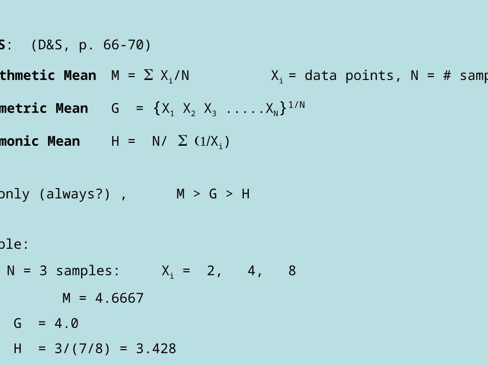
MEANS: (D&S, p. 66-70)
Arithmetic Mean M = Xi/N Xi = data points, N = # samples
Geometric Mean G = {X1 X2 X3 .....XN}1/N
Harmonic Mean H = N/ Xi)
Commonly (always?) , M > G > H
Example:
N = 3 samples: Xi = 2, 4, 8
M = 4.6667
G = 4.0
H = 3/(7/8) = 3.428
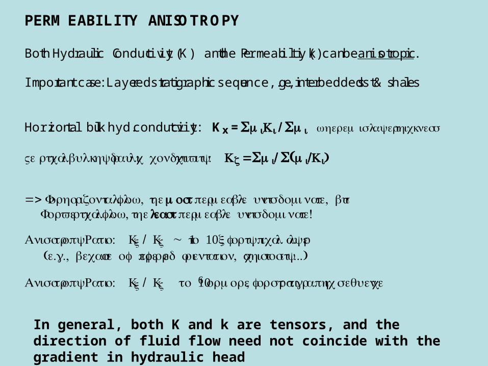
In general, both K and k are tensors, and the direction of fluid flow need not coincide with the gradient in hydraulic head
PERMEABILITY ANISOTROPY
Both Hydraulic Conductivity (K) and the Permeability (k) can be anisotropic.
Important case: Layered stratigraphic sequence, e.g., interbedded sst & shales
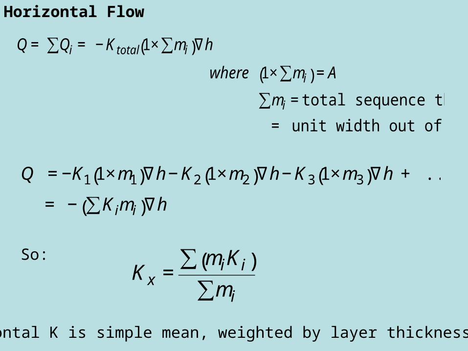
Horizontal bulk hyd. conductivity: Kx = miK i / mi w here mis l ayerthickness
Vertica l bulk hydrauli c conductivity: Kz = mi/ (mi/K i)
=> For horizontal fl ,ow t hemost permeabl e units dominate, but For vertical flow, the least permeabl e units dominate!
Anisotropy Ratio: Kx / Kz ~ t o x, for typica l layer( .e g., becaus e of preferr ed orientation, schistosity...)
Anisotropy Ratio: Kx / Kz to 6 ormore, for stratigraphic sequence
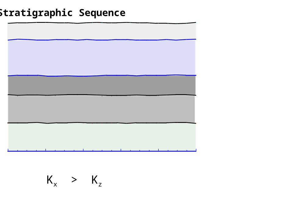
Stratigraphic Sequence
Kx > Kz
€
Kx =miKi( )∑mi∑
€
Q = Qi∑ = − K total 1× mi∑( )∇h
where 1× mi∑( ) = A
mi∑ = total sequence thickness
1 = unit width out of page
€
Q = −K1 1×m1( )∇h − K2 1×m2( )∇h − K3 1×m3( )∇h + .....
= − Kimi∑( )∇h
So:
Horizontal K is simple mean, weighted by layer thickness
Horizontal Flow

€
Kx =miKi( )∑mi∑
Stratigraphic Sequence
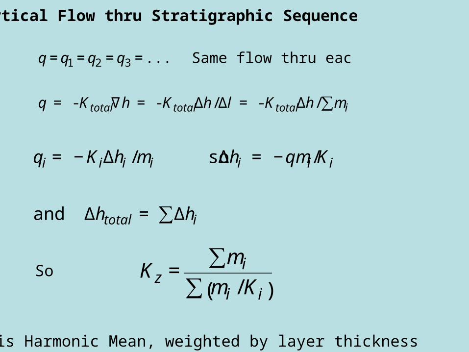
€
Kz =mi∑
mi / Ki( )∑
€
q = q1 = q2 = q3 = ... Same flow thru each layer
q = - K total∇h = - K totalΔh /Δl = - K totalΔh / mi∑
€
qi = − KiΔhi /mi so Δhi = −qmi/Ki
and Δhtotal = Δhi∑
So
Vertical Flow thru Stratigraphic Sequence
Kz is Harmonic Mean, weighted by layer thickness

€
Kx =miKi( )∑mi∑
€
Kz =mi∑
mi / Ki( )∑
Stratigraphic Sequence

PERMEABILITY ANISOTROPY
Justification: For vertical flow, Flux must be the same thru each layer! (see F&C, p. 33-34)
q = Kz,bulk (∆h/m)
= K1 (∆h1/m1) = K2 (∆h2/m2) = ....... = Kn (∆hn/mn)
=> Kz,bulk = q m/ ∆h = q m/ (∆h1 + ∆h2 + .... + ∆hn)
= q m/ (q m1/K1 + q m2/K2 + .... + q mn/Kn) =
= m / mi/Ki )
=> For horizontal flow, the most permeable units dominate, but For vertical flow, the least permeable units dominate!
Anisotropy Ratio: Kx / Kz ~ 1 to 10x, for typical layer (e.g., because of preferred orientation, schistosity...)
Anisotropy Ratio: Kx / Kz up to 106 or more, for stratigraphic sequence
In general, for layered anisotropy: Kx > Kz
However, for fracture-related anisotropy, commonly Kz > Kx

End

AquifersSaturated geologic formations with sufficient porosity and permeability k to allow significant water transmission under ordinary hydraulic gradients.
Normally, k ≥ 0.01 d
e.g., Unconsolidated sands & gravels; Sandstone, Limestone, fractured volcanics & fractured crystalline rocks
AquitardGeologic formations with low permeability that can store ground water and allow some transmission, but in an amount insufficient for production.
Less permeable layers in stratigraphic sequence;
= Leaky confining layer
e.g., clays, shales, unfractured crystalline rocks
AquicludeSaturated geologic unit incapable of transmitting significant water
Rare.
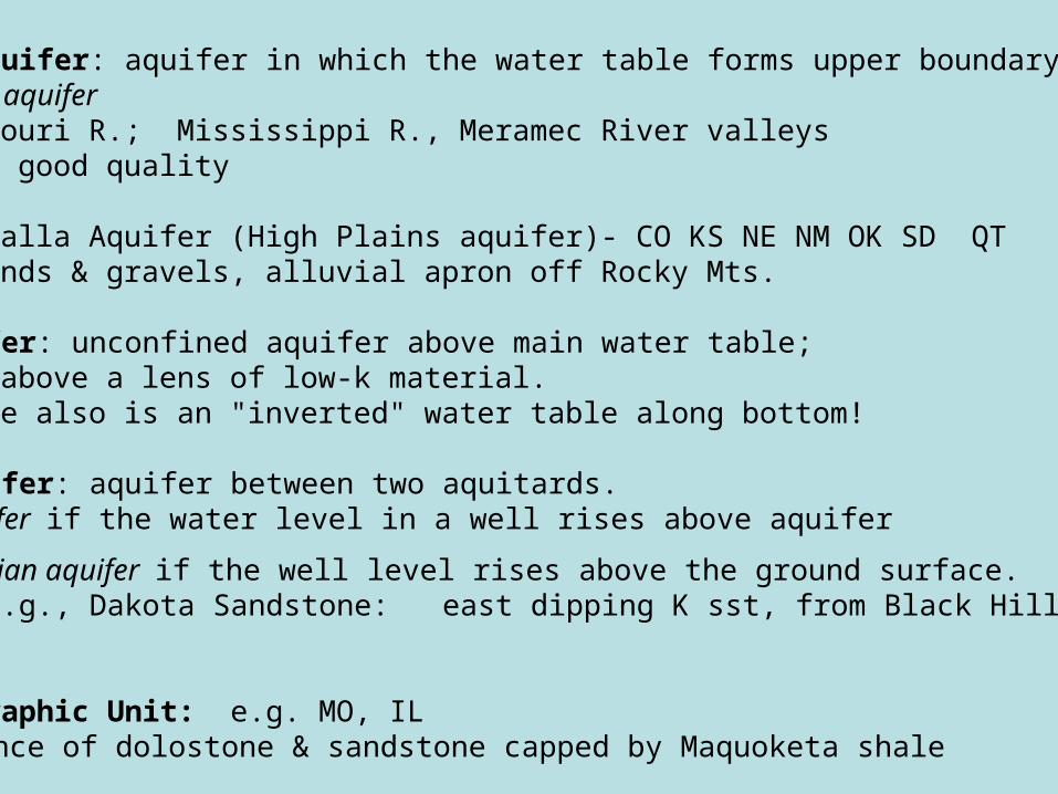
Unconfined Aquifer: aquifer in which the water table forms upper boundary. = water table aquifer e.g., Missouri R.; Mississippi R., Meramec River valleys Hi yields, good quality
e.g., Ogalalla Aquifer (High Plains aquifer)- CO KS NE NM OK SD QT Sands & gravels, alluvial apron off Rocky Mts.
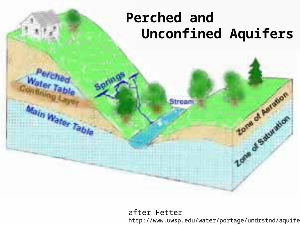
Perched Aquifer: unconfined aquifer above main water table; Generally above a lens of low-k material. Note- there also is an "inverted" water table along bottom!
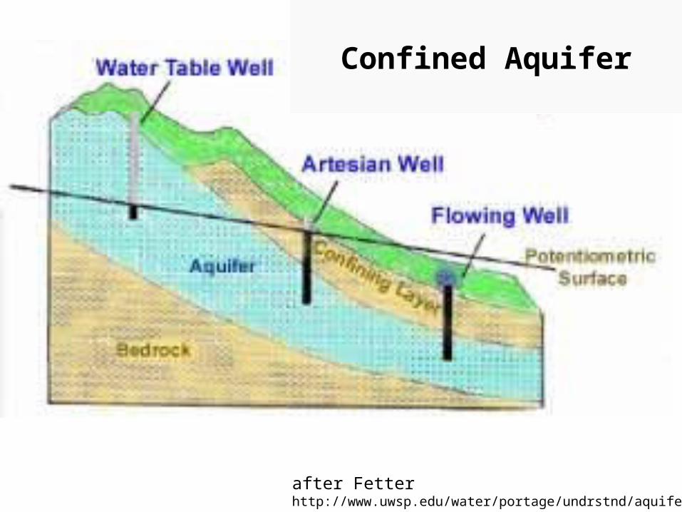
Confined Aquifer: aquifer between two aquitards. = Artesian aquifer if the water level in a well rises above aquifer
= Flowing Artesian aquifer if the well level rises above the ground surface. e.g., Dakota Sandstone: east dipping K sst, from Black Hills- artesian)
Hydrostratigraphic Unit: e.g. MO, IL C-Ord sequence of dolostone & sandstone capped by Maquoketa shale

after Driscoll, FG (1986) http://www.uwsp.edu/water/portage/undrstnd/aquifer.htm

after Fetterhttp://www.uwsp.edu/water/portage/undrstnd/aquifer.htm
Unconfined Aquifer
after Fetterhttp://www.uwsp.edu/water/portage/undrstnd/aquifer.htm
Perched and Unconfined Aquifers
after Fetterhttp://www.uwsp.edu/water/portage/undrstnd/aquifer.htm
Confined Aquifer
Hubbert (1940)
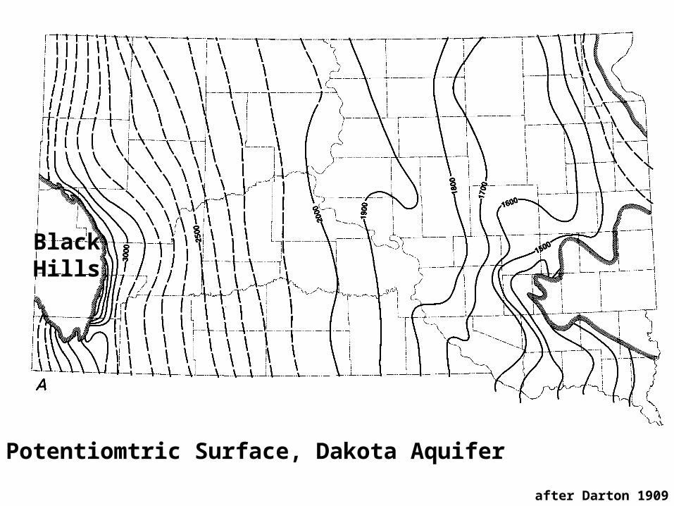
after Darton 1909
Potentiomtric Surface, Dakota Aquifer
BlackHills
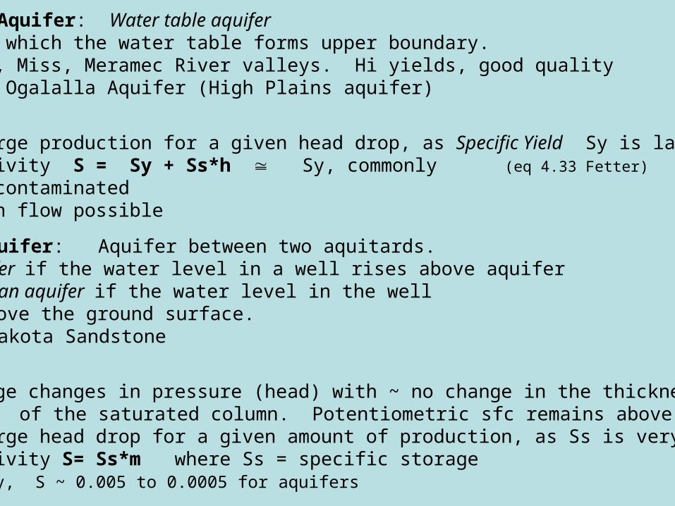
Unconfined Aquifer: Water table aquifer Aquifer in which the water table forms upper boundary.
e.g., MO, Miss, Meramec River valleys. Hi yields, good quality e.g., Ogalalla Aquifer (High Plains aquifer)
Properties: 1) Get large production for a given head drop, as Specific Yield Sy is large (~0.25).
2) Storativity S = Sy + Ss*h Sy, commonly (eq 4.33 Fetter)
3) Easily contaminated4) Artesian flow possible
Confined Aquifer: Aquifer between two aquitards. Artesian aquifer if the water level in a well rises above aquiferFlowing Artesian aquifer if the water level in the well
rises above the ground surface. e.g., Dakota Sandstone
Properties: 1) Get large changes in pressure (head) with ~ no change in the thickness
of the saturated column. Potentiometric sfc remains above the unit. 2) Get large head drop for a given amount of production, as Ss is very small.3) Storativity S= Ss*m where Ss = specific storage
Commonly, S ~ 0.005 to 0.0005 for aquifers
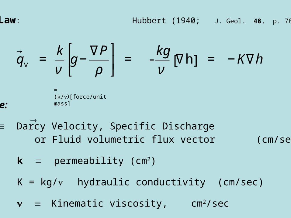
Darcy's Law: Hubbert (1940; J. Geol. 48, p. 785-944)
where:
qv Darcy Velocity, Specific Discharge or Fluid volumetric flux vector (cm/sec)
k permeability (cm2)
K = kg/ hydraulic conductivity (cm/sec)
Kinematic viscosity, cm2/sec
€
qv = k
νg −
∇P
ρ
⎡
⎣ ⎢
⎤
⎦ ⎥ = -
kg
ν∇h[ ] = − K∇h
= (k/[force/unit mass]

Gravitational Potential g
€
g =GM
r
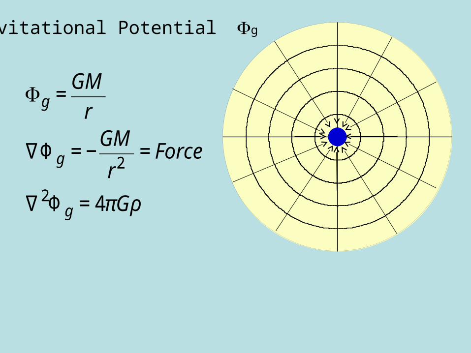
Gravitational Potential g
€
g =GM
r
∇Φg = −GM
r2= Force
∇2Φg = 4πGρ
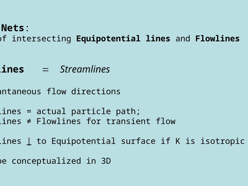
Flow Nets: Set of intersecting Equipotential lines and Flowlines
Flowlines Streamlines
Instantaneous flow directions Pathlines = actual particle path; Pathlines ≠ Flowlines for transient flow
. Flowlines | to Equipotential surface if K is isotropic
Can be conceptualized in 3D

Fetter
No Flow
No
Flow
No Flow
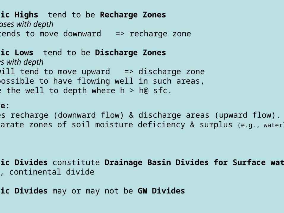
Topographic Highs tend to be Recharge Zones h decreases with depth Water tends to move downward => recharge zone
Topographic Lows tend to be Discharge Zones h increases with depth Water will tend to move upward => discharge zone It is possible to have flowing well in such areas,
if case the well to depth where h > h@ sfc.
Hinge Line: Separates recharge (downward flow) & discharge areas (upward flow).
Can separate zones of soil moisture deficiency & surplus (e.g., waterlogging).
Topographic Divides constitute Drainage Basin Divides for Surface water
e.g., continental divide
Topographic Divides may or may not be GW Divides
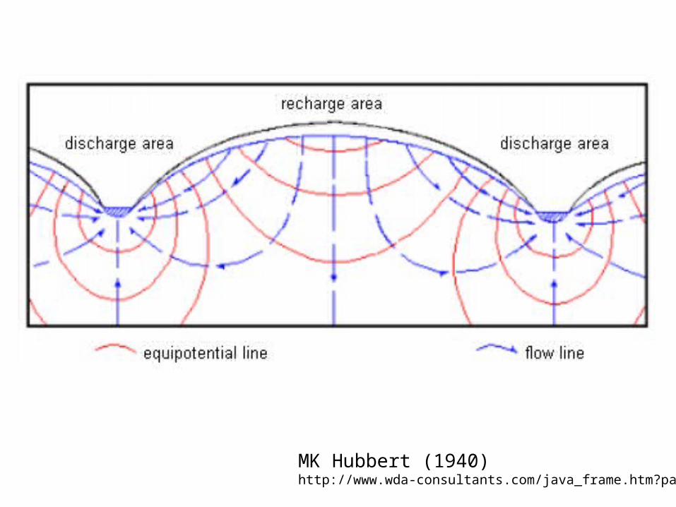
MK Hubbert (1940)http://www.wda-consultants.com/java_frame.htm?page17
Fetter, after Hubbert (1940)

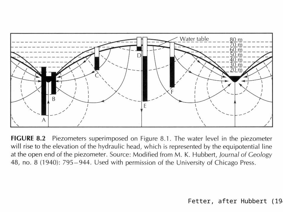
Equipotential LinesLines of constant head. Contours on potentiometric surface or on water table map
=> Equipotential Surface in 3D
Potentiometric Surface: ("Piezometric sfc") Map of the hydraulic head;
Contours are equipotential lines Imaginary surface representing the level to which water would
rise in a nonpumping well cased to an aquifer, representing vertical projection of equipotential surface to land sfc.
Vertical planes assumed; no vertical flow: 2D representation of a 3D phenomenonConcept rigorously valid only for horizontal flow w/i horizontal aquifer
Measure w/ Piezometers small dia non-pumping well with short screen-can measure hydraulic head at a point (Fetter, p. 134)
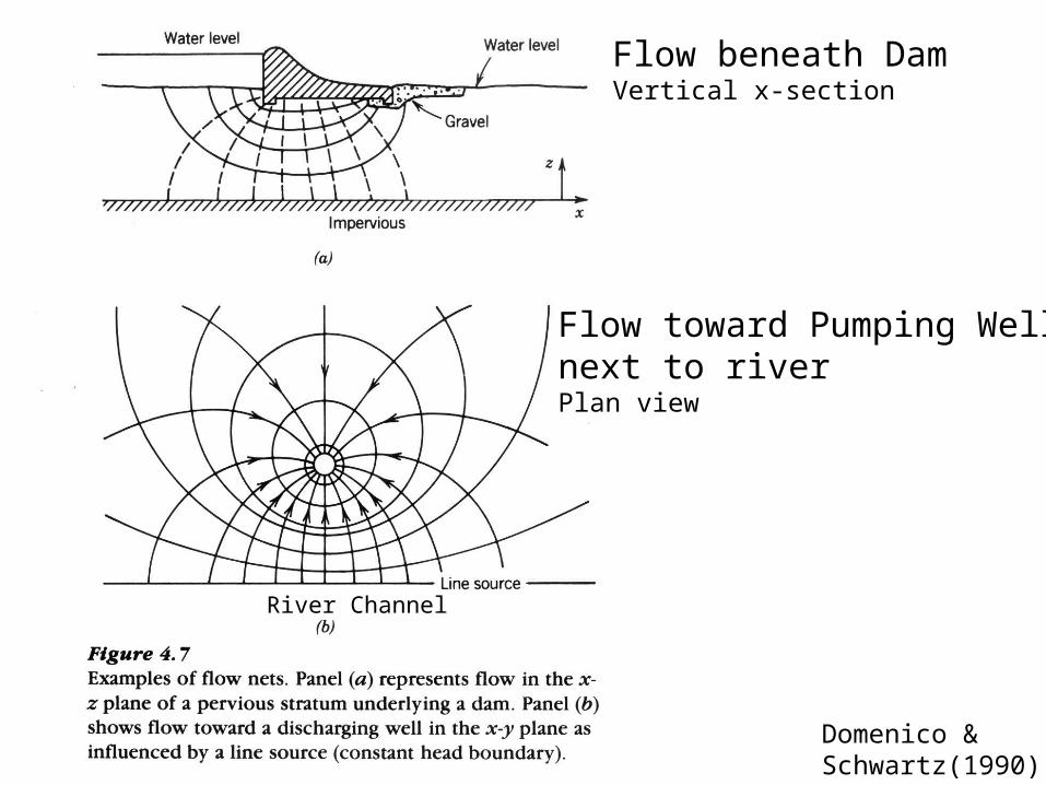
Domenico & Schwartz(1990)
Flow beneath DamVertical x-section
Flow toward Pumping Well,next to riverPlan view
River Channel
after Freeze and Witherspoon 1967http://wlapwww.gov.bc.ca/wat/gws/gwbc/!!gwbc.html
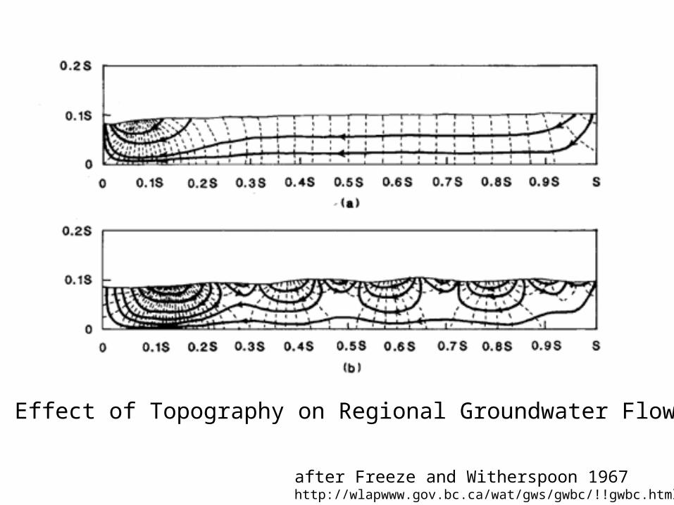
Effect of Topography on Regional Groundwater Flow
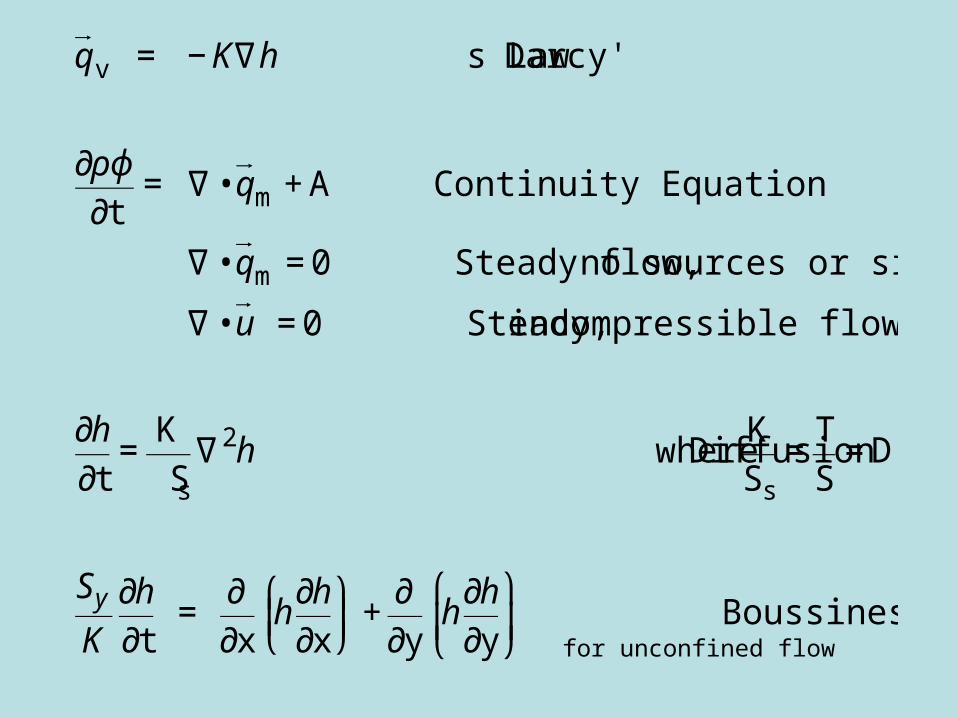
€
qv = − K∇h Darcy' s Law
∂ρϕ∂t
= ∇ • qm + A Continuity Equation
∇ • qm = 0 Steady flow, no sources or sinks
∇ • u = 0 Steady, incompressible flow
∂h∂t
=K Ss
∇2h Diffusion Eq., where KSs
=TS
= D
Sy
K∂h∂t
= ∂∂x
h∂h∂x
⎛ ⎝ ⎜
⎞ ⎠ ⎟ +
∂∂y
h∂h∂y
⎛
⎝ ⎜
⎞
⎠ ⎟ Boussinesq Eq.
for unconfined flow
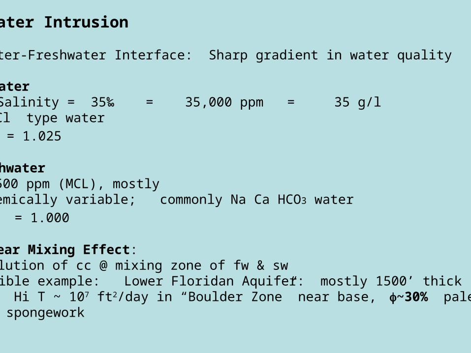
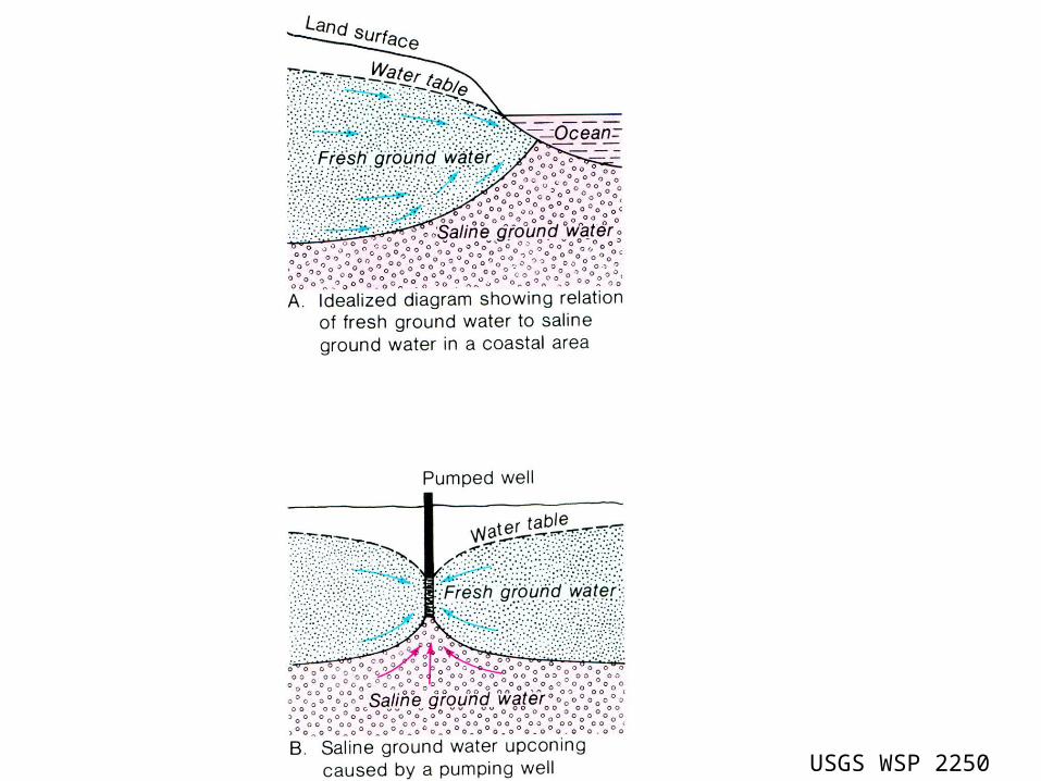
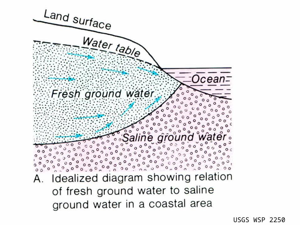
Saltwater Intrusion
Saltwater-Freshwater Interface: Sharp gradient in water quality
Seawater Salinity = 35‰ = 35,000 ppm = 35 g/l
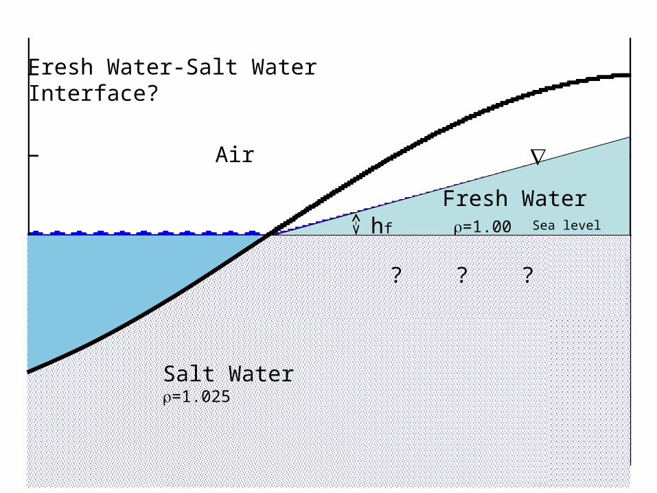
NaCl type water sw = 1.025
Freshwater
< 500 ppm (MCL), mostly Chemically variable; commonly Na Ca HCO3 waterfw = 1.000
Nonlinear Mixing Effect: Dissolution of cc @ mixing zone of fw & sw
Possible example: Lower Floridan Aquifer: mostly 1500’ thick Very Hi T ~ 107 ft2/day in “Boulder Zone” near base, ~30% paleokarst?Cave spongework
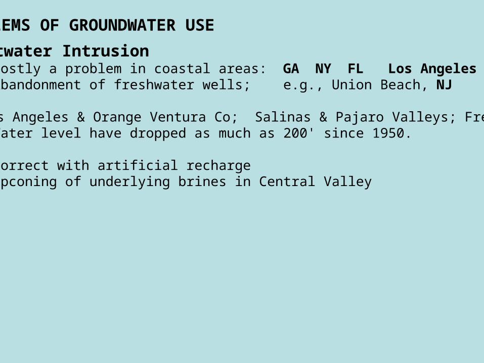
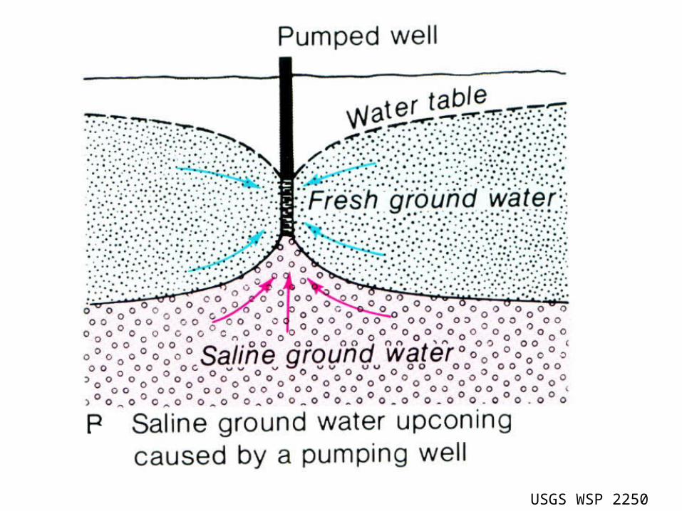
PROBLEMS OF GROUNDWATER USE
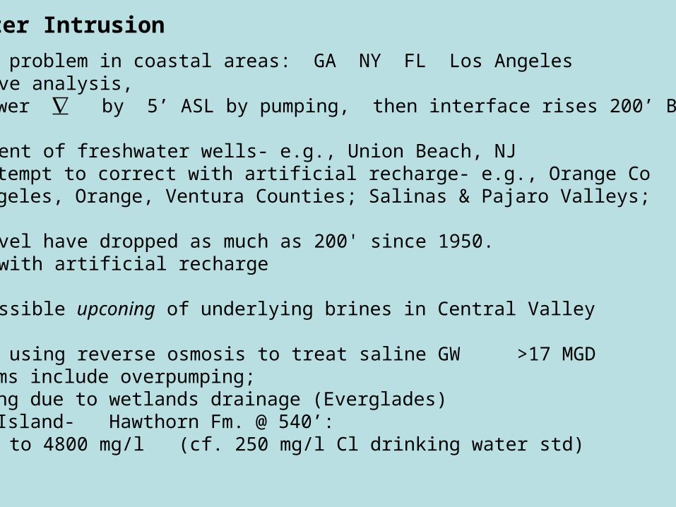
Saltwater IntrusionMostly a problem in coastal areas: GA NY FL Los AngelesAbandonment of freshwater wells; e.g., Union Beach, NJ
Los Angeles & Orange Ventura Co; Salinas & Pajaro Valleys; FremontWater level have dropped as much as 200' since 1950.
Correct with artificial rechargeUpconing of underlying brines in Central Valley
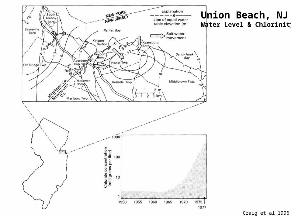
Craig et al 1996
Union Beach, NJWater Level & Chlorinity
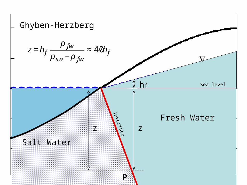
Ghyben-Herzberg
Air
Fresh Water =1.00hf
Fresh Water-Salt Water Interface?
Sea level
Salt Water=1.025
? ? ?

Ghyben-Herzberg
Salt Water
Fresh Water
hf
z
Ghyben-Herzberg
P
Sea level
zinterface

€
P = gzρ sw = g(h f + z)ρ fw
z = h fρ fw
ρ sw −ρ fw
≈ 40h f
Ghyben-Herzberg Analysis
Hydrostatic Condition P - g = 0 No horizontal P gradients
Note: z = depth fw = 1.00 sw= 1.025
Ghyben-Herzberg
Salt Water
Fresh Water
hf
z
Ghyben-Herzberg
P
Sea level
zinterface
€
z = h fρ fw
ρ sw −ρ fw
≈ 40h f
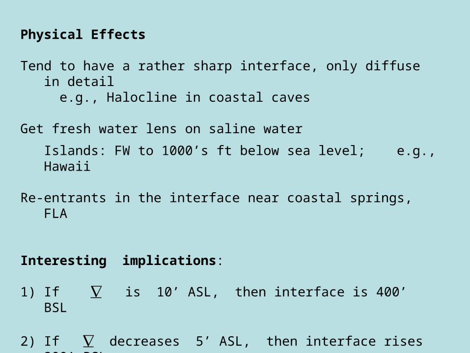
Physical Effects
Tend to have a rather sharp interface, only diffuse in detail e.g., Halocline in coastal caves Get fresh water lens on saline water
Islands: FW to 1000’s ft below sea level; e.g., Hawaii
Re-entrants in the interface near coastal springs, FLA
Interesting implications:
1) If is 10’ ASL, then interface is 400’ BSL
2) If decreases 5’ ASL, then interface rises 200’ BSL
3) Slope of interface ~ 40 x slope of water table

Hubbert’s (1940) Analysis
Hydrodynamic condition with immiscible fluid interface
1) If hydrostatic conditions existed: All FW would have drained outWater table @ sea level, everywhere w/ SW below
2) G-H analysis underestimates the depth to the interface
Assume interface between two immiscible fluids Each fluid has its own potential h everywhere,
even where that fluid is not present!
FW potentials are horizontal in static SW and air zones, where heads for latter phases are constant
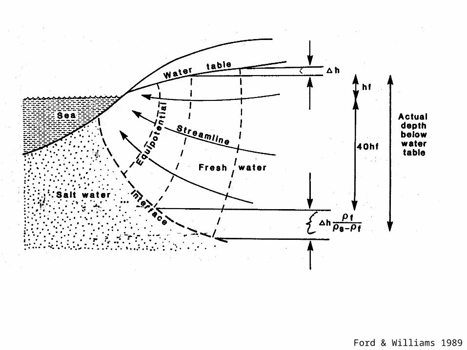
Ford & Williams 1989
….
..

after Ford & Williams 1989
….
..
Fresh Water Equipotentials
Fresh Water Equipotentials
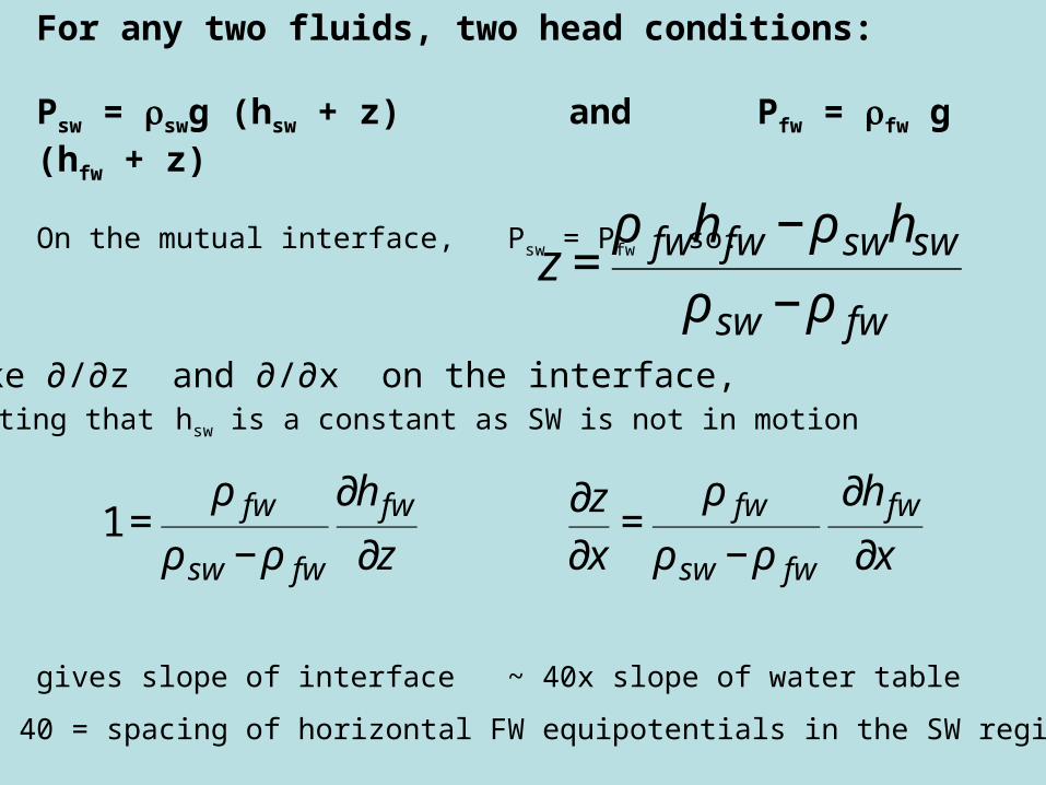
For any two fluids, two head conditions:
Psw = swg (hsw + z) and Pfw = fw g (hfw + z)
On the mutual interface, Psw = Pfw so:
€
1 =ρ fw
ρ sw −ρ fw
∂h fw
∂z
∂z∂x
=ρ fw
ρ sw −ρ fw
∂h fw
∂x
€
€
z =ρ fwh fw −ρ swhsw
ρ sw −ρ fw
∂z/∂x gives slope of interface ~ 40x slope of water table
Also, 40 = spacing of horizontal FW equipotentials in the SW region
Take ∂/∂z and ∂/∂x on the interface, noting that hsw is a constant as SW is not in motion
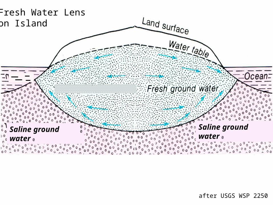
after USGS WSP 2250
Saline ground water 000
Fresh Water Lenson Island
Saline ground water 0
Confined
Unconfined
Fetter
Saltwater Intrusion
Mostly a problem in coastal areas: GA NY FL Los AngelesFrom above analysis,
if lower by 5’ ASL by pumping, then interface rises 200’ BSL!
Abandonment of freshwater wells- e.g., Union Beach, NJCan attempt to correct with artificial recharge- e.g., Orange CoLos Angeles, Orange, Ventura Counties; Salinas & Pajaro Valleys;
Water level have dropped as much as 200' since 1950. Correct with artificial recharge
Also, possible upconing of underlying brines in Central Valley
FLA- now using reverse osmosis to treat saline GW >17 MGD Problems include overpumping;
upconing due to wetlands drainage (Everglades) Marco Island- Hawthorn Fm. @ 540’:
Cl to 4800 mg/l (cf. 250 mg/l Cl drinking water std)

Possible Solutions
Artificial Recharge (most common)
Reduced Pumping
Pumping trough
Artificial pressure ridge
Subsurface Barrier

End
USGS WSP 2250
USGS WSP 2250
USGS WSP 2250
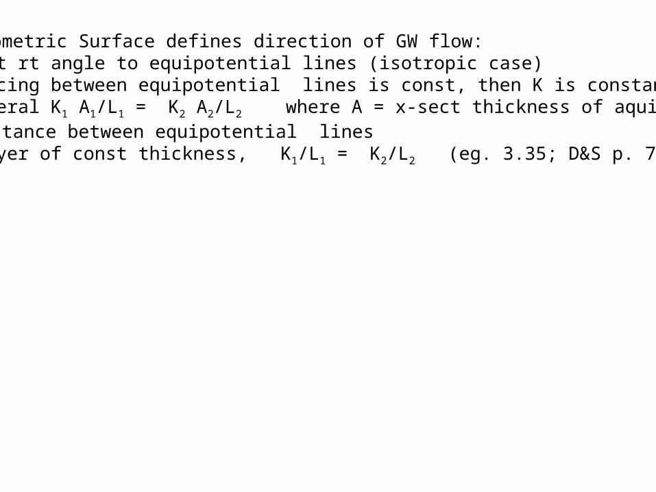
Potentiometric Surface defines direction of GW flow: Flow at rt angle to equipotential lines (isotropic case)If spacing between equipotential lines is const, then K is constantIn general K1 A1/L1 = K2 A2/L2 where A = x-sect thickness of aquifer;
L = distance between equipotential linesFor layer of const thickness, K1/L1 = K2/L2 (eg. 3.35; D&S p. 79)
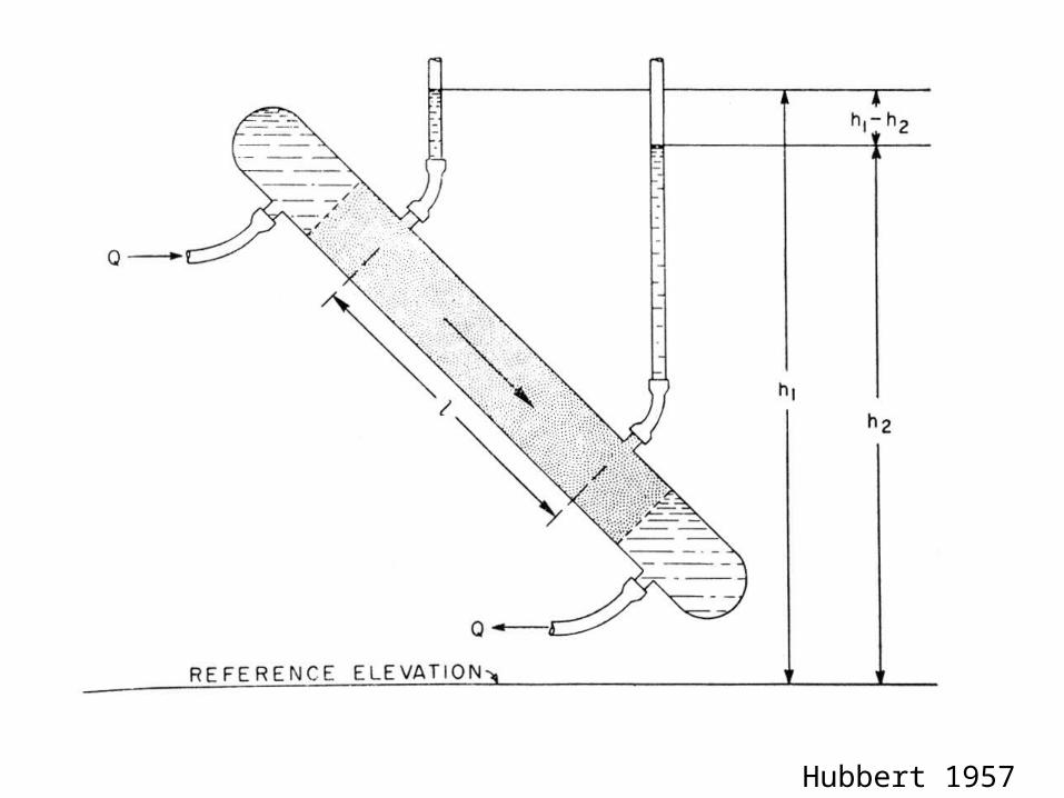
Hubbert 1957
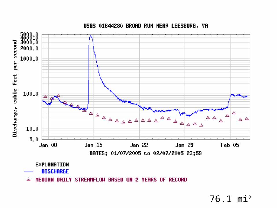
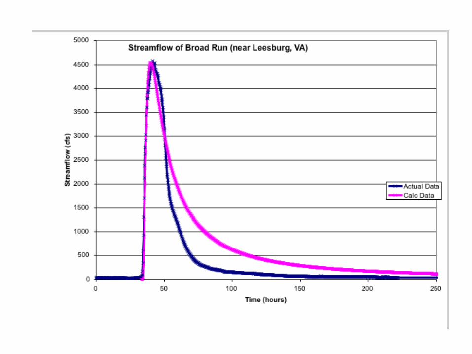
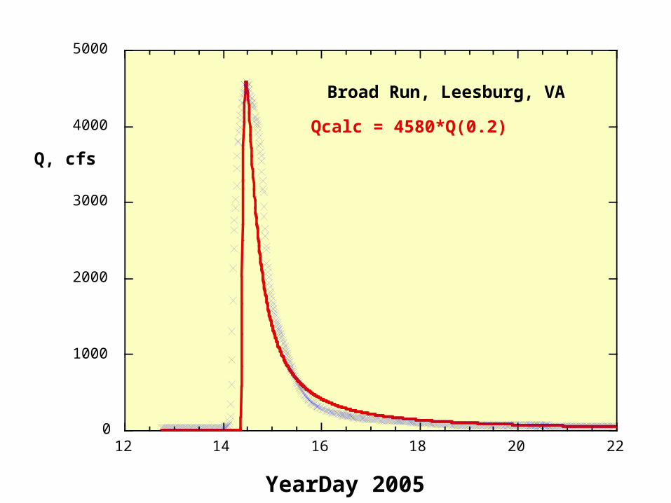
76.1 mi2
0
1000
2000
3000
4000
5000
12 14 16 18 20 22
Broad Run, Leesburg, VA
Q, cfs
YearDay 2005
Qcalc = 4580*Q(0.2)
14.7
14.8
14.9
15
15.1
15.2
15.3
1 1.5 2 2.5 3 3.5 4
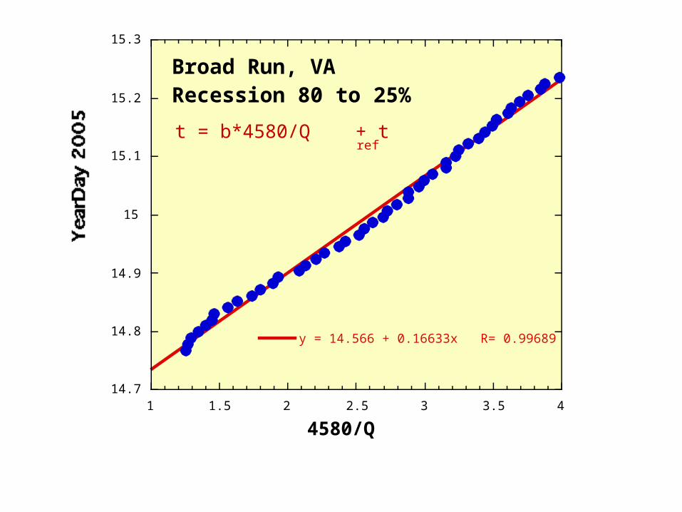
Broad Run, VARecession 80 to 25%
y = 14.566 + 0.16633x R= 0.99689
4580/Q
t = b*4580/Q + tref
3
4
5
6
7
8
9
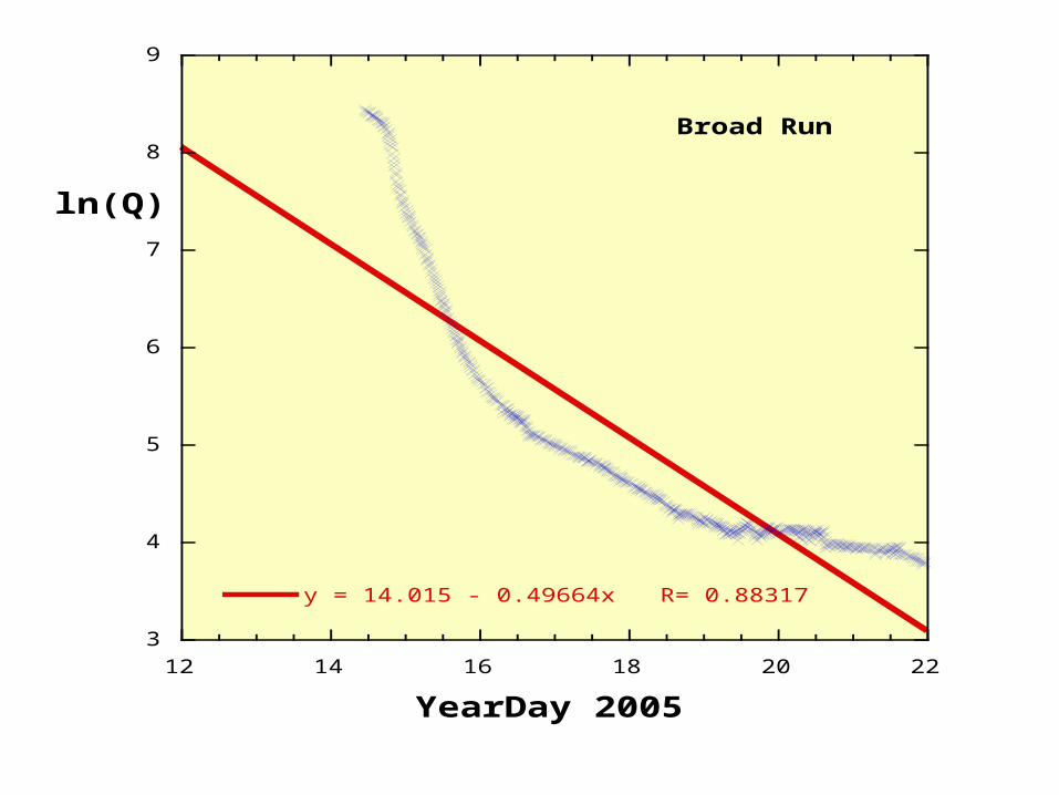
12 14 16 18 20 22
Broad Run
y = 14.015 - 0.49664x R= 0.88317
ln(Q)
YearDay 2005

0
1000
2000
3000
4000
5000
2 3 4 5 6 7 8 9 10
Broad Run
Q, cfs
Stage, ft
Q=1343-796.44 S +123.31 S2 R=.9996

0
1000
2000
3000
4000
5000
6000
7000
2 3 4 5 6 7 8 9
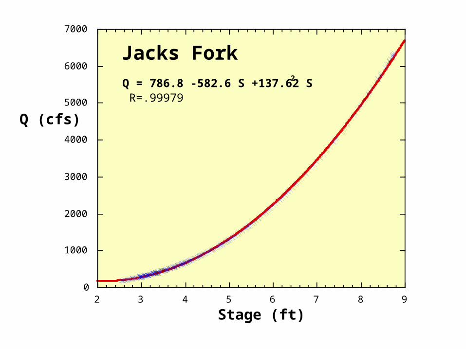
Q = 786.8 -582.6 S +137.62 S2 R=.99979
Q (cfs)
Stage (ft)
Jacks Fork
13.6
13.8
14
14.2
14.4
14.6
14.8
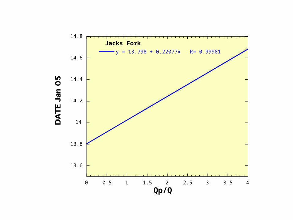
0 0.5 1 1.5 2 2.5 3 3.5 4
Jacks Fork y = 13.798 + 0.22077x R= 0.99981
Qp/Q
0
1000
2000
3000
4000
5000
6000
7000
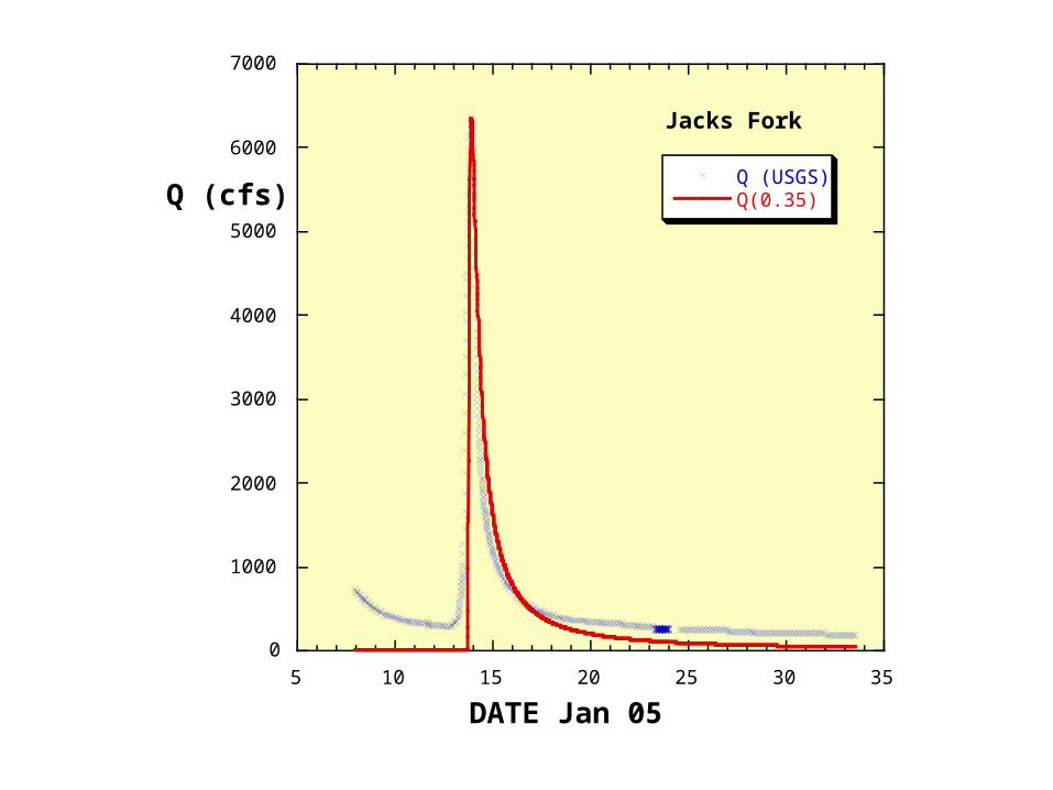
5 10 15 20 25 30 35
Jacks Fork
Q (USGS)Q(0.35)Q (cfs)
DATE Jan 05
0
1000
2000
3000
4000
5000
6000
7000 0
0.2
0.4
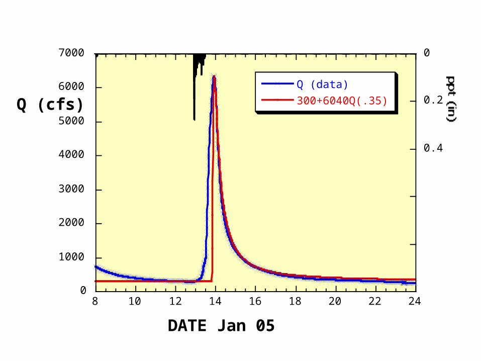
8 10 12 14 16 18 20 22 24
JacksFork in MOQ (data)
300+6040Q(.35)Q (cfs)
DATE Jan 05


0
1000
2000
3000
4000
5000
6000
7000
5 10 15 20 25 30 35
Jacks Fork
Q (USGS)Q(0.35)Q (cfs)
DATE Jan 05
FLUID DYNAMICS Consider flow of homogeneous fluid of constant densityFluid transport in the Earth's crust is dominated by
Viscous, laminar flow, thru minute cracks and openings, Slow enough that inertial effects are negligible.
What drives flow within a porous medium? Down hill?
Down Pressure? Down Head?
Consider:Case 1: Artesian well- fluid flows uphill. Case 2: Swimming pool- large vertical P gradient, but no flow. Case3: Convective gyre w/i Swimming pool-
ascending fluid moves from hi to lo P descending fluid moves from low to hi P
Case 4: Metamorphic rocks and magmatic systems.
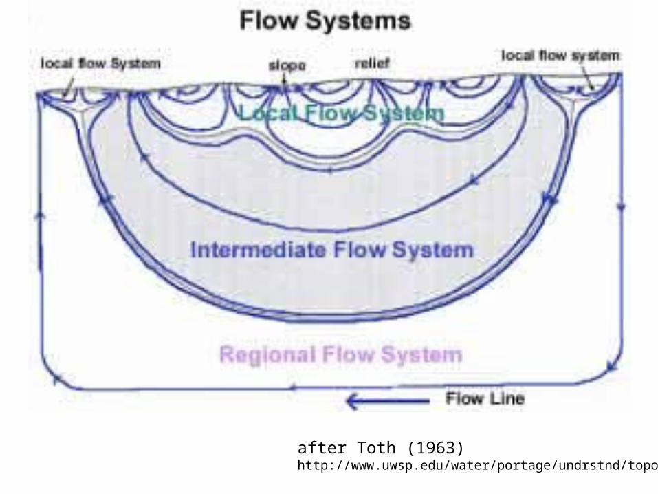
after Toth (1963)http://www.uwsp.edu/water/portage/undrstnd/topo.htm

Fetter, after Toth (1963)

Ghyben-Herzberg
Salt Water
Fresh Water
hf
z
€
z = h fρ fw
ρ sw −ρ fw
≈ 40h f
Ghyben-Herzberg
P
Sea level