Fluid Mechanics Prof. T.I. Eldho Department of Civil...
30
Fluid Mechanics Prof. T.I. Eldho Department of Civil Engineering Indian Institute of Technology, Bombay Lecture - 2 Fundamental Concepts of Fluid Flow and Fluid Statics Welcome back to the video lecture on fluid mechanics. In the first lecture, we have discussed the introductory aspects of fluid mechanics We have discussed about the various fluid properties, various theories used in fluid mechanics and how it will be used in our this video course; we discussed the various fundamental theories which applicable in the case of fluid mechanics; we discussed the various flow visualization techniques, used in fluid mechanics and the flow lines like stream lines, path lines and streak lines. Today, in this lecture, first we will discuss about the classification of fluids. (Refer Slide Time: 22:18) As I mentioned earlier, the fluids can be classified according to various fluid properties, fluid behavior or the dimensions on which they will be dealing with the fluids or the fluid problem which we are dealing. So, mainly the fluids fluid flow can be classified according to the rhelogical consideration, spatial dimensions, dilational tensor, then
-
Upload
dinhnguyet -
Category
Documents
-
view
219 -
download
0
Transcript of Fluid Mechanics Prof. T.I. Eldho Department of Civil...
Fluid Mechanics
Prof. T.I. Eldho
Department of Civil Engineering
Indian Institute of Technology, Bombay
Lecture - 2
Fundamental Concepts of Fluid Flow and Fluid Statics
Welcome back to the video lecture on fluid mechanics. In the first lecture, we have
discussed the introductory aspects of fluid mechanics We have discussed about the
various fluid properties, various theories used in fluid mechanics and how it will be used
in our this video course; we discussed the various fundamental theories which applicable
in the case of fluid mechanics; we discussed the various flow visualization techniques,
used in fluid mechanics and the flow lines like stream lines, path lines and streak lines.
Today, in this lecture, first we will discuss about the classification of fluids.
(Refer Slide Time: 22:18)
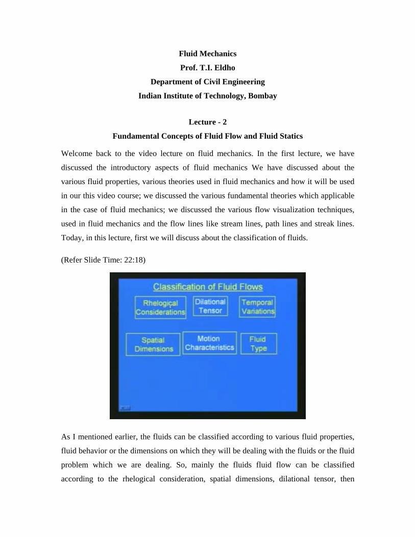
As I mentioned earlier, the fluids can be classified according to various fluid properties,
fluid behavior or the dimensions on which they will be dealing with the fluids or the fluid
problem which we are dealing. So, mainly the fluids fluid flow can be classified
according to the rhelogical consideration, spatial dimensions, dilational tensor, then
motion characteristics, the temporal variations and fluid types. Here, we will discuss in
detail about the various types of fluid flow according to various aspects.
(Refer Slide Time: 2:53)
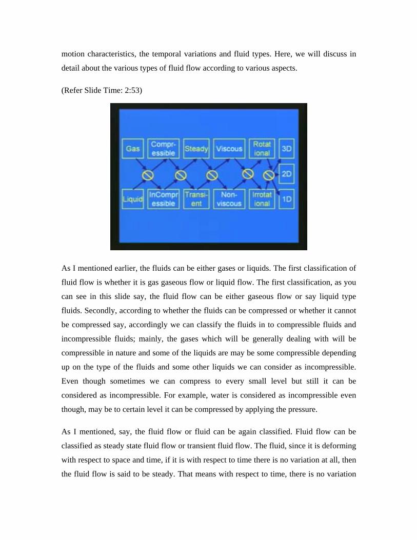
As I mentioned earlier, the fluids can be either gases or liquids. The first classification of
fluid flow is whether it is gas gaseous flow or liquid flow. The first classification, as you
can see in this slide say, the fluid flow can be either gaseous flow or say liquid type
fluids. Secondly, according to whether the fluids can be compressed or whether it cannot
be compressed say, accordingly we can classify the fluids in to compressible fluids and
incompressible fluids; mainly, the gases which will be generally dealing with will be
compressible in nature and some of the liquids are may be some compressible depending
up on the type of the fluids and some other liquids we can consider as incompressible.
Even though sometimes we can compress to every small level but still it can be
considered as incompressible. For example, water is considered as incompressible even
though, may be to certain level it can be compressed by applying the pressure.
As I mentioned, say, the fluid flow or fluid can be again classified. Fluid flow can be
classified as steady state fluid flow or transient fluid flow. The fluid, since it is deforming
with respect to space and time, if it is with respect to time there is no variation at all, then
the fluid flow is said to be steady. That means with respect to time, there is no variation
of the fluid properties but the fluid properties like velocity or depth a flow all this fluid
properties are constants with respect to time and there is no variation with respect to time.
In the case of UN study flow or transient flow the fluid property like velocity, pressure
and depth, all these parameters are varying with respect to time. So, these types of fluids
are called unsteady fluid flow or transient flow. As we discussed earlier the viscosity is
an important fluid property. So, accordingly, whether the fluid flow which we are dealing
with has got viscosity or the viscosity is negligible or there is no viscosity, then
accordingly we can classify the fluids into viscous fluids or viscous flow and non-viscous
flow or invest flow. So according to the variation or according to the fluid has viscosity
fluid is called viscous fluid flow and then if viscosity is not considered then that kind of
fluid is called non-viscous or invest fluid flow.
If there is any circulation or any rotation aspect as far as the fluid flow is concerned we
can classify the fluid into rotational fluid or irrotational fluid. In the case of rotational
fluid, there can be circulation there can be vorticity and all other parameters but as far as
irrotational fluid is concerned circulation is not there and vorticity is 0. So, those fluids
are called irrotational fluid or irrotational fluid flow.
According to the space we are considering 3 dimension, x, y and z. We can classify the
fluid as 3 dimension fluid flow or 2 dimension fluid flow or 1 dimension fluid flow. As
all of you know fluid flow is definitely 3 dimensional in nature as you can see any type of
fluid flow is 3 dimension nature.
(Refer Slide Time: 06:51)
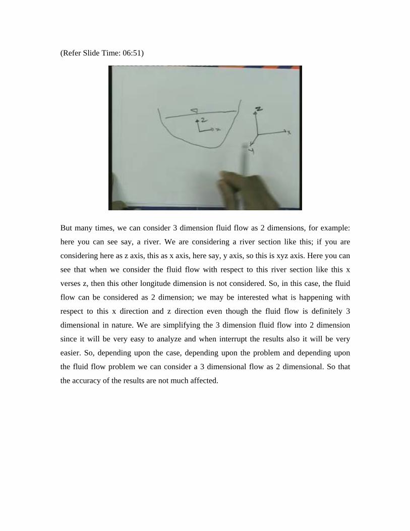
But many times, we can consider 3 dimension fluid flow as 2 dimensions, for example:
here you can see say, a river. We are considering a river section like this; if you are
considering here as z axis, this as x axis, here say, y axis, so this is xyz axis. Here you can
see that when we consider the fluid flow with respect to this river section like this x
verses z, then this other longitude dimension is not considered. So, in this case, the fluid
flow can be considered as 2 dimension; we may be interested what is happening with
respect to this x direction and z direction even though the fluid flow is definitely 3
dimensional in nature. We are simplifying the 3 dimension fluid flow into 2 dimension
since it will be very easy to analyze and when interrupt the results also it will be very
easier. So, depending upon the case, depending upon the problem and depending upon
the fluid flow problem we can consider a 3 dimensional flow as 2 dimensional. So that
the accuracy of the results are not much affected.
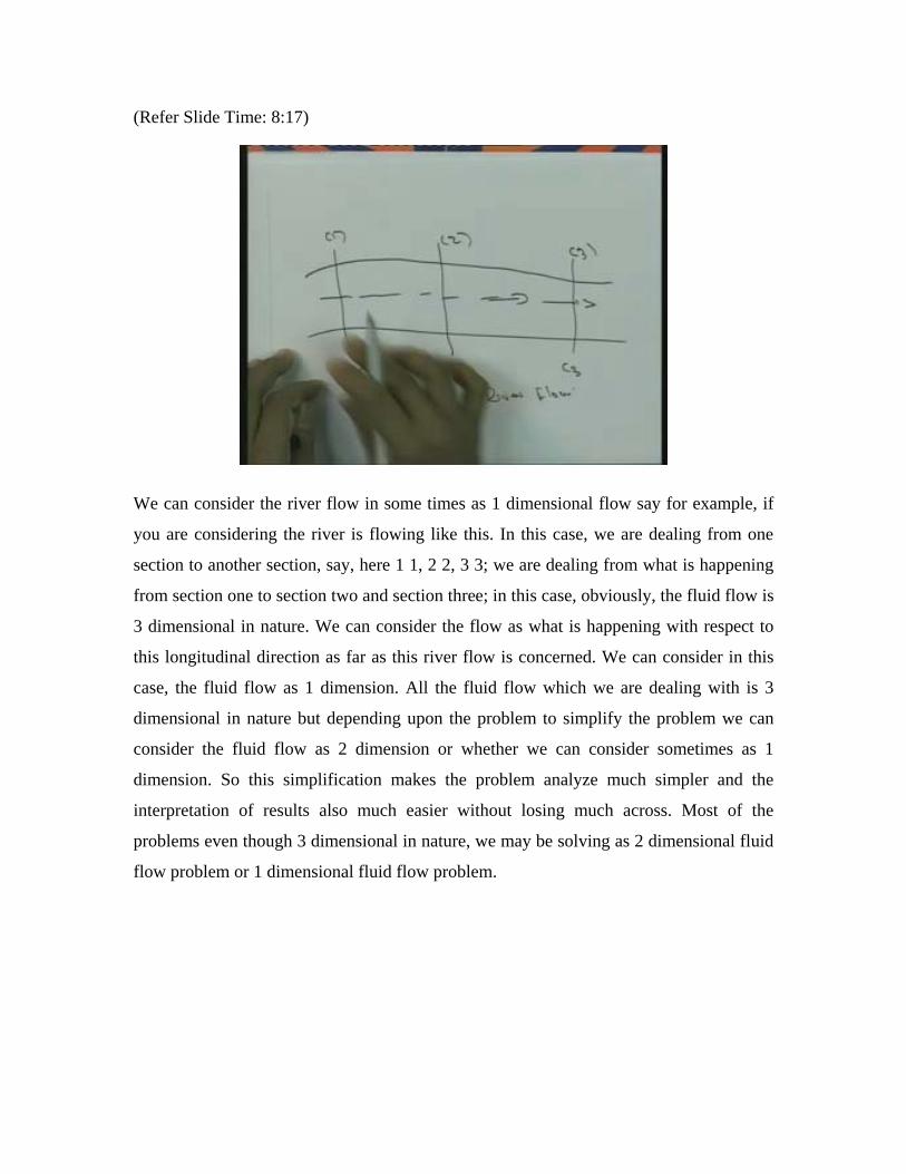
(Refer Slide Time: 8:17)
We can consider the river flow in some times as 1 dimensional flow say for example, if
you are considering the river is flowing like this. In this case, we are dealing from one
section to another section, say, here 1 1, 2 2, 3 3; we are dealing from what is happening
from section one to section two and section three; in this case, obviously, the fluid flow is
3 dimensional in nature. We can consider the flow as what is happening with respect to
this longitudinal direction as far as this river flow is concerned. We can consider in this
case, the fluid flow as 1 dimension. All the fluid flow which we are dealing with is 3
dimensional in nature but depending upon the problem to simplify the problem we can
consider the fluid flow as 2 dimension or whether we can consider sometimes as 1
dimension. So this simplification makes the problem analyze much simpler and the
interpretation of results also much easier without losing much across. Most of the
problems even though 3 dimensional in nature, we may be solving as 2 dimensional fluid
flow problem or 1 dimensional fluid flow problem.
(Refer Slide Time: 9:36)
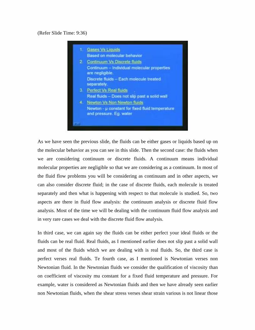
As we have seen the previous slide, the fluids can be either gases or liquids based up on
the molecular behavior as you can see in this slide. Then the second case: the fluids when
we are considering continuum or discrete fluids. A continuum means individual
molecular properties are negligible so that we are considering as a continuum. In most of
the fluid flow problems you will be considering as continuum and in other aspects, we
can also consider discrete fluid; in the case of discrete fluids, each molecule is treated
separately and then what is happening with respect to that molecule is studied. So, two
aspects are there in fluid flow analysis: the continuum analysis or discrete fluid flow
analysis. Most of the time we will be dealing with the continuum fluid flow analysis and
in very rare cases we deal with the discrete fluid flow analysis.
In third case, we can again say the fluids can be either perfect your ideal fluids or the
fluids can be real fluid. Real fluids, as I mentioned earlier does not slip past a solid wall
and most of the fluids which we are dealing with is real fluids. So, the third case is
perfect verses real fluids. Te fourth case, as I mentioned is Newtonian verses non
Newtonian fluid. In the Newtonian fluids we consider the qualification of viscosity than
on coefficient of viscosity mu constant for a fixed fluid temperature and pressure. For
example, water is considered as Newtonian fluids and then we have already seen earlier
non Newtonian fluids, when the shear stress verses shear strain various is not linear those
fluids are non Newtonian fluids and then the non Newtonian fluids as I mentioned in the
mu varies, say, for example, milk is a non Newtonian fluid
(Refer Slide Time: 11:29)
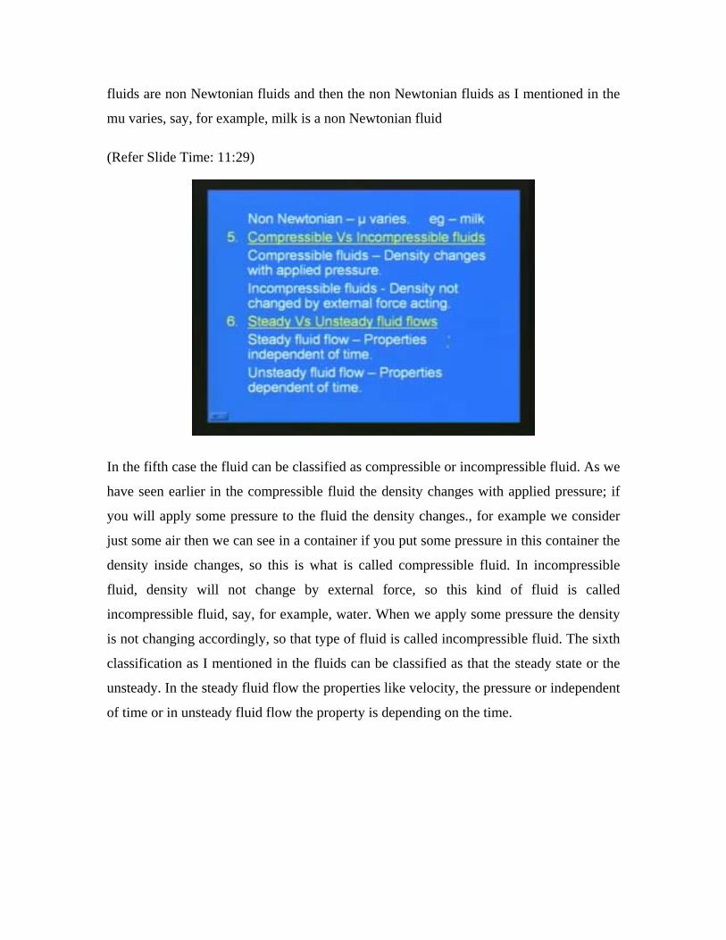
In the fifth case the fluid can be classified as compressible or incompressible fluid. As we
have seen earlier in the compressible fluid the density changes with applied pressure; if
you will apply some pressure to the fluid the density changes., for example we consider
just some air then we can see in a container if you put some pressure in this container the
density inside changes, so this is what is called compressible fluid. In incompressible
fluid, density will not change by external force, so this kind of fluid is called
incompressible fluid, say, for example, water. When we apply some pressure the density
is not changing accordingly, so that type of fluid is called incompressible fluid. The sixth
classification as I mentioned in the fluids can be classified as that the steady state or the
unsteady. In the steady fluid flow the properties like velocity, the pressure or independent
of time or in unsteady fluid flow the property is depending on the time.
(Refer Slide Time: 12:30)
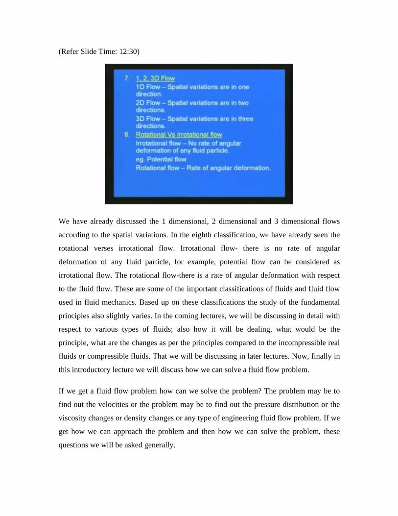
We have already discussed the 1 dimensional, 2 dimensional and 3 dimensional flows
according to the spatial variations. In the eighth classification, we have already seen the
rotational verses irrotational flow. Irrotational flow- there is no rate of angular
deformation of any fluid particle, for example, potential flow can be considered as
irrotational flow. The rotational flow-there is a rate of angular deformation with respect
to the fluid flow. These are some of the important classifications of fluids and fluid flow
used in fluid mechanics. Based up on these classifications the study of the fundamental
principles also slightly varies. In the coming lectures, we will be discussing in detail with
respect to various types of fluids; also how it will be dealing, what would be the
principle, what are the changes as per the principles compared to the incompressible real
fluids or compressible fluids. That we will be discussing in later lectures. Now, finally in
this introductory lecture we will discuss how we can solve a fluid flow problem.
If we get a fluid flow problem how can we solve the problem? The problem may be to
find out the velocities or the problem may be to find out the pressure distribution or the
viscosity changes or density changes or any type of engineering fluid flow problem. If we
get how we can approach the problem and then how we can solve the problem, these
questions we will be asked generally.
(Refer Slide Time: 14:32)
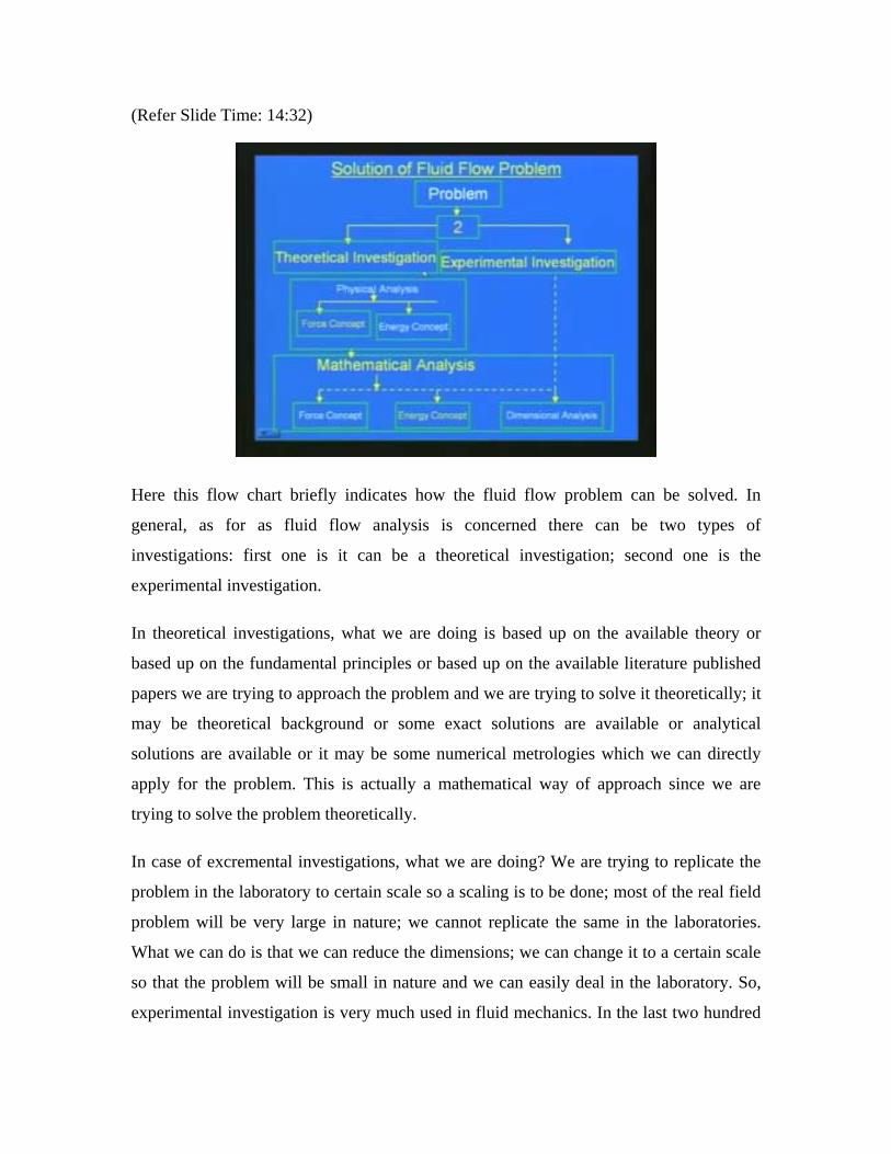
Here this flow chart briefly indicates how the fluid flow problem can be solved. In
general, as for as fluid flow analysis is concerned there can be two types of
investigations: first one is it can be a theoretical investigation; second one is the
experimental investigation.
In theoretical investigations, what we are doing is based up on the available theory or
based up on the fundamental principles or based up on the available literature published
papers we are trying to approach the problem and we are trying to solve it theoretically; it
may be theoretical background or some exact solutions are available or analytical
solutions are available or it may be some numerical metrologies which we can directly
apply for the problem. This is actually a mathematical way of approach since we are
trying to solve the problem theoretically.
In case of excremental investigations, what we are doing? We are trying to replicate the
problem in the laboratory to certain scale so a scaling is to be done; most of the real field
problem will be very large in nature; we cannot replicate the same in the laboratories.
What we can do is that we can reduce the dimensions; we can change it to a certain scale
so that the problem will be small in nature and we can easily deal in the laboratory. So,
experimental investigation is very much used in fluid mechanics. In the last two hundred
to three hundred years experimental fluid mechanics is very much developed in the
solution of various problems. As far as the experimental investigations are concerned
there are certain limitations. The limitations are: it is very expensive in nature and we
have to do the scaling; through the scaling certain aspects of the problems may not be
able to replicate in the laboratory. So certain level of the reality of the problem may be
last in the replications of the laboratory and then running the model in the laboratory, the
accuracy may be reduced. So, experimental investigations have certain limitations but if
theoretical investigations or analytical solutions are not available then it has got some
limitations, the accuracy again may be reduced. Now, as far as theoretical investigations
are concerned how are we approaching the problem? If the engineering fluid flow
problem is given then first we can understand the problem in a physical nature, what is
the problem, what are the inputs data available and what are the outputs expected what
the physical principles are based up on the problem which we have to investigate. So this
analysis is called the physical analysis.
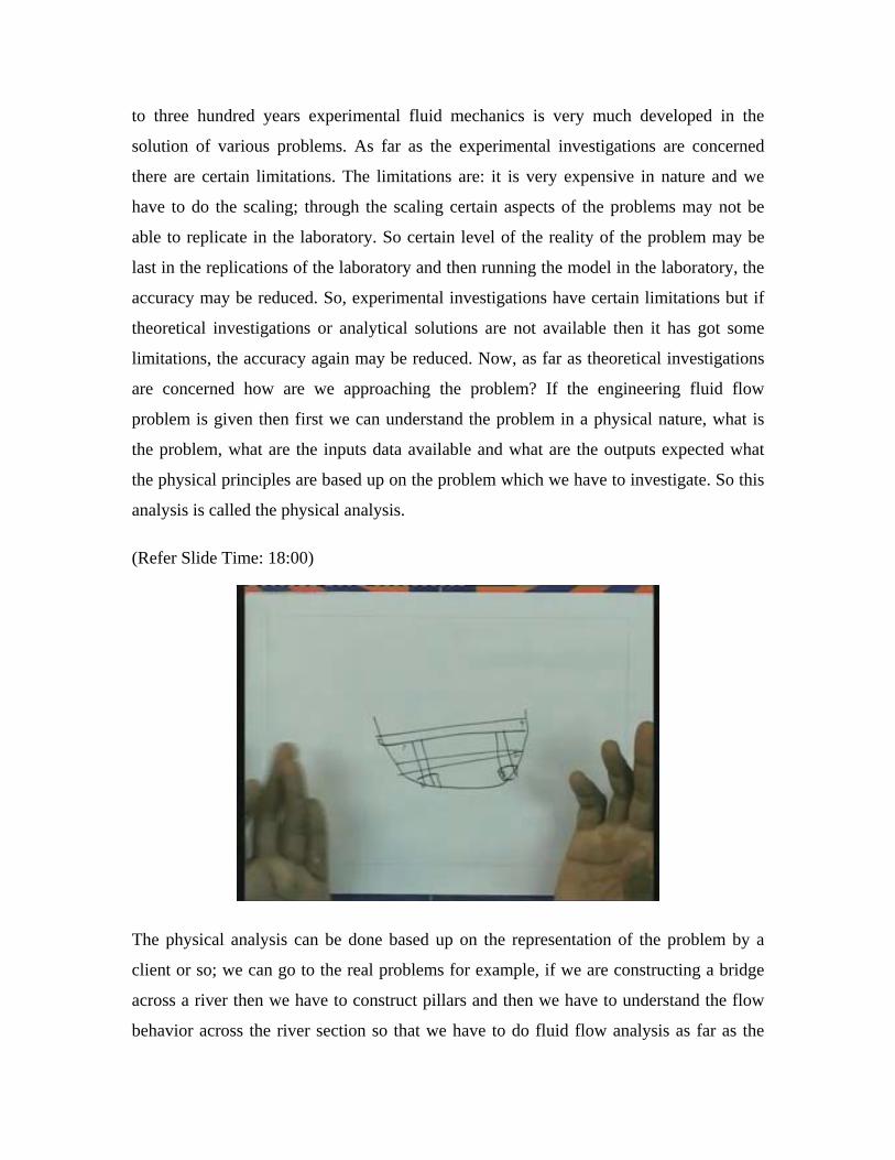
(Refer Slide Time: 18:00)
The physical analysis can be done based up on the representation of the problem by a
client or so; we can go to the real problems for example, if we are constructing a bridge
across a river then we have to construct pillars and then we have to understand the flow
behavior across the river section so that we have to do fluid flow analysis as far as the
section is concerned where the bridge is constructed. We may go to the field and see how
the river is flowing, what are the important parameters which we have to deal here. We
have to analyze and we have to understand the problem physically. So we may have to go
to the field or we have to analyze in our office depending up on the data available given
by the client.
For example when we are going to construct a bridge across the river, we have to see
depending up on the monsoon or depending upon the rain fall through out the year how
the water level will be varying, how it is increasing or how it is decreasing and then what
will be the flow velocity at the particular location. We are going to construct the bridge
the bridge and then the bank of the river has any motion problems or all these things we
have to analyze physically. This is called physical analysis. In the case of fluid mechanics
analysis this physical analysis can be based up on the force concept or energy concept.
The force concept means we will analyze what are the forces acting on the particular
problem which we have dealing with and then how it is going to affect the fluid flow
properties or the particular variable which we are going to understand and the second
concept is called energy concept, how energy variations are like here as they would be
the energy creations; we will be analyzing how it will be affecting the particular problem
so the physical analysis is very important in the solution of any fluid flow problem.
Physical analysis generally can be there upon the force concept or based up on the energy
concept. After this physical analysis is over we can understand the problem in which way
we have to approach the problem and we can try to make a mathematical formulation of
the problem. After this physical analysis next step is the mathematical analysis. In the
mathematical analysis with respect to the physical analysis we already know what will be
the domain of the problem which we will be dealing.
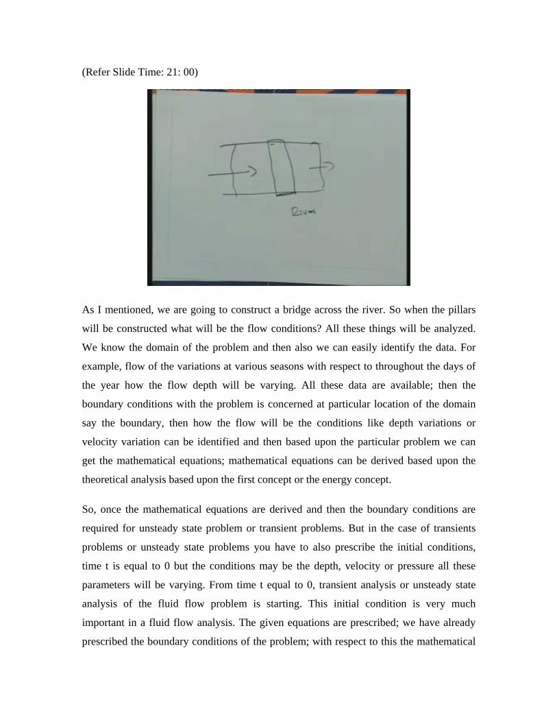
(Refer Slide Time: 21: 00)
As I mentioned, we are going to construct a bridge across the river. So when the pillars
will be constructed what will be the flow conditions? All these things will be analyzed.
We know the domain of the problem and then also we can easily identify the data. For
example, flow of the variations at various seasons with respect to throughout the days of
the year how the flow depth will be varying. All these data are available; then the
boundary conditions with the problem is concerned at particular location of the domain
say the boundary, then how the flow will be the conditions like depth variations or
velocity variation can be identified and then based upon the particular problem we can
get the mathematical equations; mathematical equations can be derived based upon the
theoretical analysis based upon the first concept or the energy concept.
So, once the mathematical equations are derived and then the boundary conditions are
required for unsteady state problem or transient problems. But in the case of transients
problems or unsteady state problems you have to also prescribe the initial conditions,
time t is equal to 0 but the conditions may be the depth, velocity or pressure all these
parameters will be varying. From time t equal to 0, transient analysis or unsteady state
analysis of the fluid flow problem is starting. This initial condition is very much
important in a fluid flow analysis. The given equations are prescribed; we have already
prescribed the boundary conditions of the problem; with respect to this the mathematical
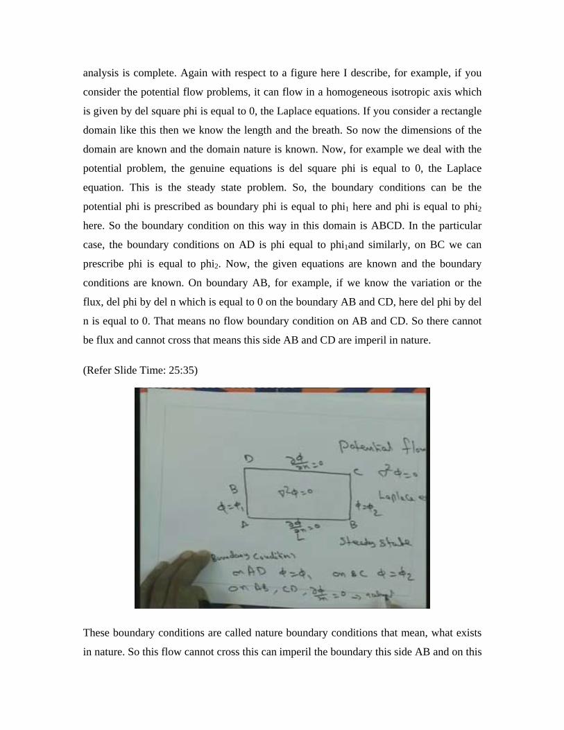
analysis is complete. Again with respect to a figure here I describe, for example, if you
consider the potential flow problems, it can flow in a homogeneous isotropic axis which
is given by del square phi is equal to 0, the Laplace equations. If you consider a rectangle
domain like this then we know the length and the breath. So now the dimensions of the
domain are known and the domain nature is known. Now, for example we deal with the
potential problem, the genuine equations is del square phi is equal to 0, the Laplace
equation. This is the steady state problem. So, the boundary conditions can be the
potential phi is prescribed as boundary phi is equal to phi1 here and phi is equal to phi2
here. So the boundary condition on this way in this domain is ABCD. In the particular
case, the boundary conditions on AD is phi equal to phi1and similarly, on BC we can
prescribe phi is equal to phi2. Now, the given equations are known and the boundary
conditions are known. On boundary AB, for example, if we know the variation or the
flux, del phi by del n which is equal to 0 on the boundary AB and CD, here del phi by del
n is equal to 0. That means no flow boundary condition on AB and CD. So there cannot
be flux and cannot cross that means this side AB and CD are imperil in nature.
(Refer Slide Time: 25:35)
These boundary conditions are called nature boundary conditions that mean, what exists
in nature. So this flow cannot cross this can imperil the boundary this side AB and on this
side CD, so these conditions are called nature conditions or [25:48 ] and the boundary
conditions which we prescribed on AD and BC are called divisional boundary conditions
or direct boundary conditions.
So as far as this potential flow problem is concerned the mathematical analysis or
mathematical statement is over since we have only described the domain, we have
already described the boundary condition and we have already described the given
equations. Now, with respect to this, we can solve this problem either we can get
analytical solution depending upon the problem or we can solve the problem numerically
so depending upon the case.
This is about the mathematical analysis and as I mentioned in the experimental
investigation we have to replicate the real problem in the laboratory and then with respect
to certain scale we will be running the experiment what is happening in the field that will
be done in the laboratory. Then we will be taking some readings sometimes it can be say
either the velocity measurements are the depth variations or pressure measurements or
this measurements will be done experimentally in the laboratory. Then to have some
specific relationships we can give some dimensional analysis as mentioned in this slide
here. (Refer Slide Time 27:10). Dimensional analysis is also very important in
experimental investigation as well as mathematical investigations. So, dimensions with
respect to the bucking phi theorem or various theorems, we will discuss about this
dimensional analysis later.
In summary, in this introductory lecture on fluid mechanics, we have discussed the
various aspects of fluid flow and the various fluid properties. We have discussed the
fundamental principles which will be used in the fluid flow analysis like the mass
consideration of momentum, consideration of energy and then we also discussed the
various fluid visualization techniques like using dies, using smoke or other metrologies.
We have discussed various metrologies of representing of a fluid flow like a stream lines,
potential line, streak lines path lines will have discussed and then we have discussed
based up on the various fluid properties we have classified the flows with respect to
space, one D flow, two D flow and three D flow or with respect to the viscosity, that is,
viscous flow or non-viscous flow and then finally, we have discussed about how we can
approach a fluid flow problem or solution to a fluid flow problem.
As I mentioned, we can approach the fluid flow problem theoretically or experimentally
and then in theoretical investigation we can derive a mathematical model by describing
the domain, then given equation in boundary condition. So this is about the introductory
lecture on this video course on fluid mechanics
In this second chapter on fluid mechanics video course, we will be discussing mainly on
fluid statics.
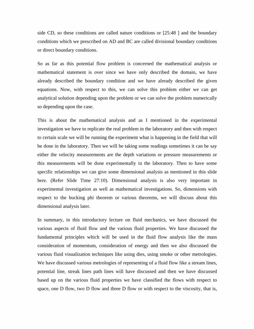
(Refer Slide Time: 29:19)
The main objectives in this section is to introduce the concepts of fluid pressure, forces
on solid surfaces, buoyant forces and related theories. Secondly, we shall see the
determination of fluid pressure and forces for various cases. Then we will emphasis in the
importance of fluid statics as far as fluid mechanics is concerned.
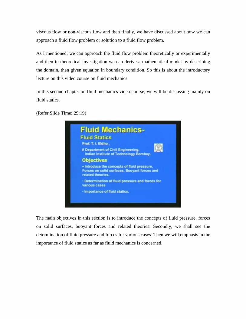
(Refer Slide Time: 30:30)
Now, as I mentioned earlier, static fluids means fluid is not moving that means fluid is in
rest. So, you can see there is some water in a small basin. Here fluid is now at rest; there
is no movement as far as the fluid is concerned; it is as far as the boundary is concerned
the fluid is at rest so that we can say the fluid is in statics conditions and the various
theories on statics will be applicable as far as a static fluid is concerned.
In solid mechanics, most of the problems we will be analyzing are in that condition. So,
most of the theories in solid mechanics are applicable for fluids at rest or static fluid. In
static fluids you can see that since fluid is not moving it is at rest here, so that there is no
shearing force. Whenever the fluid is trying to move only between the layers there will be
shearing force but as far as fluid is at rest or static fluid there is no shearing force. We
need not have to worry about the shearing force and now before going to more details of
fluid statics we will just review some aspects of forces.
(Refer Slide Time: 31:26)
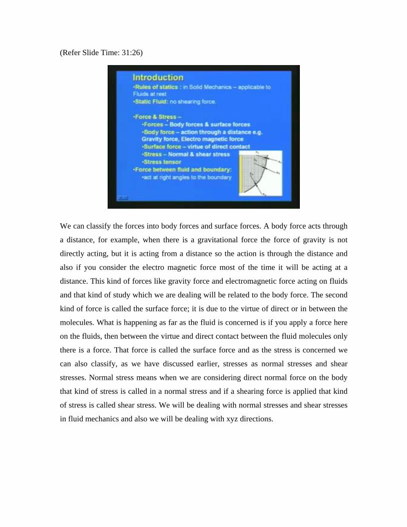
We can classify the forces into body forces and surface forces. A body force acts through
a distance, for example, when there is a gravitational force the force of gravity is not
directly acting, but it is acting from a distance so the action is through the distance and
also if you consider the electro magnetic force most of the time it will be acting at a
distance. This kind of forces like gravity force and electromagnetic force acting on fluids
and that kind of study which we are dealing will be related to the body force. The second
kind of force is called the surface force; it is due to the virtue of direct or in between the
molecules. What is happening as far as the fluid is concerned is if you apply a force here
on the fluids, then between the virtue and direct contact between the fluid molecules only
there is a force. That force is called the surface force and as the stress is concerned we
can also classify, as we have discussed earlier, stresses as normal stresses and shear
stresses. Normal stress means when we are considering direct normal force on the body
that kind of stress is called in a normal stress and if a shearing force is applied that kind
of stress is called shear stress. We will be dealing with normal stresses and shear stresses
in fluid mechanics and also we will be dealing with xyz directions.
(Refer Slide Time: 32:21)
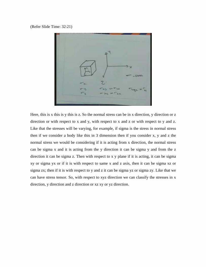
Here, this is x this is y this is z. So the normal stress can be in x direction, y direction or z
direction or with respect to x and y, with respect to x and z or with respect to y and z.
Like that the stresses will be varying, for example, if sigma is the stress in normal stress
then if we consider a body like this in 3 dimension then if you consider x, y and z the
normal stress we would be considering if it is acting from x direction, the normal stress
can be sigma x and it is acting from the y direction it can be sigma y and from the z
direction it can be sigma z. Then with respect to x y plane if it is acting, it can be sigma
xy or sigma yx or if it is with respect to same x and z axis, then it can be sigma xz or
sigma zx; then if it is with respect to y and z it can be sigma yz or sigma zy. Like that we
can have stress tensor. So, with respect to xyz direction we can classify the stresses in x
direction, y direction and z direction or xz xy or yz direction.
(Refer Slide Time: 35:22)
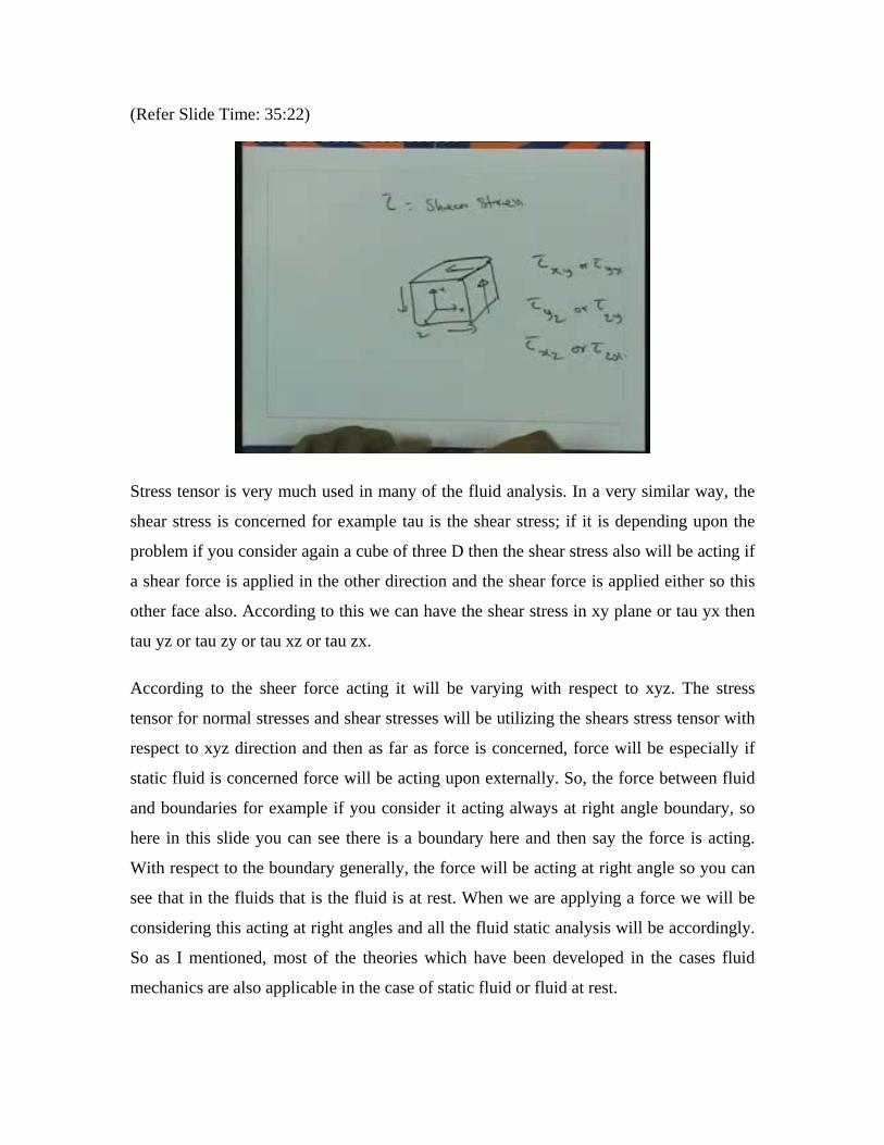
Stress tensor is very much used in many of the fluid analysis. In a very similar way, the
shear stress is concerned for example tau is the shear stress; if it is depending upon the
problem if you consider again a cube of three D then the shear stress also will be acting if
a shear force is applied in the other direction and the shear force is applied either so this
other face also. According to this we can have the shear stress in xy plane or tau yx then
tau yz or tau zy or tau xz or tau zx.
According to the sheer force acting it will be varying with respect to xyz. The stress
tensor for normal stresses and shear stresses will be utilizing the shears stress tensor with
respect to xyz direction and then as far as force is concerned, force will be especially if
static fluid is concerned force will be acting upon externally. So, the force between fluid
and boundaries for example if you consider it acting always at right angle boundary, so
here in this slide you can see there is a boundary here and then say the force is acting.
With respect to the boundary generally, the force will be acting at right angle so you can
see that in the fluids that is the fluid is at rest. When we are applying a force we will be
considering this acting at right angles and all the fluid static analysis will be accordingly.
So as I mentioned, most of the theories which have been developed in the cases fluid
mechanics are also applicable in the case of static fluid or fluid at rest.
Fluid at rest, we can consider each element for example, this basin water is at rest so
when we consider the fluid statics or static fluid here. If we consider each element then
the fluid element should be in equilibrium; there is no moment and the fluid is at rest. So,
if there are n forces acting then finally each fluid element should be in equilibrium.
(Refer Slide Time: 38:05)
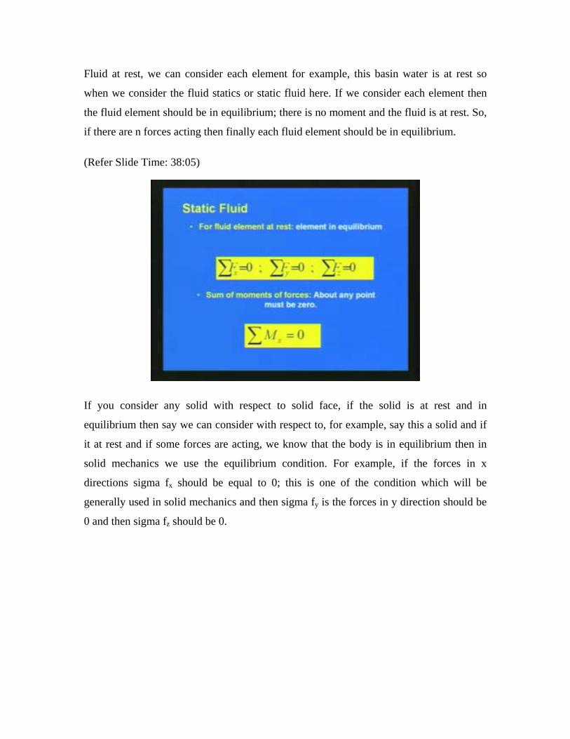
If you consider any solid with respect to solid face, if the solid is at rest and in
equilibrium then say we can consider with respect to, for example, say this a solid and if
it at rest and if some forces are acting, we know that the body is in equilibrium then in
solid mechanics we use the equilibrium condition. For example, if the forces in x
directions sigma fx should be equal to 0; this is one of the condition which will be
generally used in solid mechanics and then sigma fy is the forces in y direction should be
0 and then sigma fz should be 0.
(Refer Slide Time: 39:07)
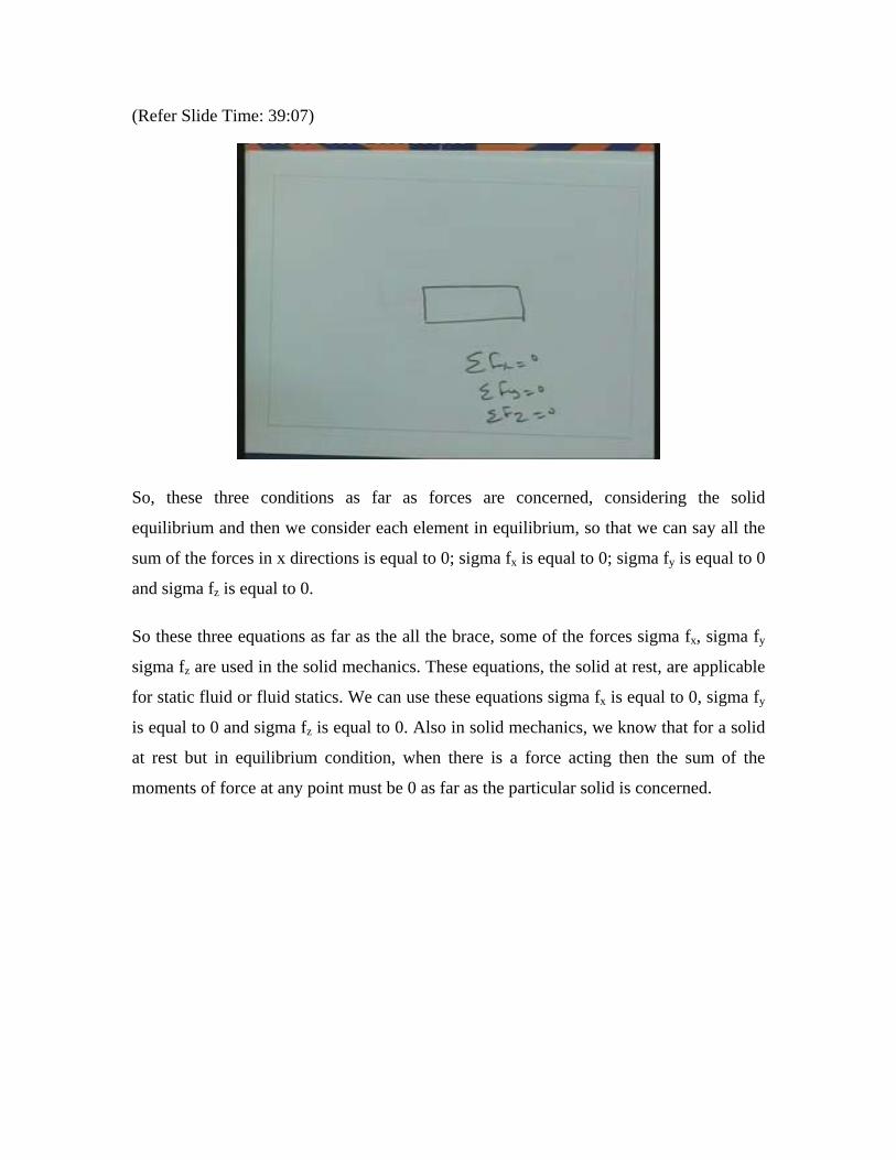
So, these three conditions as far as forces are concerned, considering the solid
equilibrium and then we consider each element in equilibrium, so that we can say all the
sum of the forces in x directions is equal to 0; sigma fx is equal to 0; sigma fy is equal to 0
and sigma fz is equal to 0.
So these three equations as far as the all the brace, some of the forces sigma fx, sigma fy
sigma fz are used in the solid mechanics. These equations, the solid at rest, are applicable
for static fluid or fluid statics. We can use these equations sigma fx is equal to 0, sigma fy
is equal to 0 and sigma fz is equal to 0. Also in solid mechanics, we know that for a solid
at rest but in equilibrium condition, when there is a force acting then the sum of the
moments of force at any point must be 0 as far as the particular solid is concerned.
(Refer Slide Time: 40: 28)
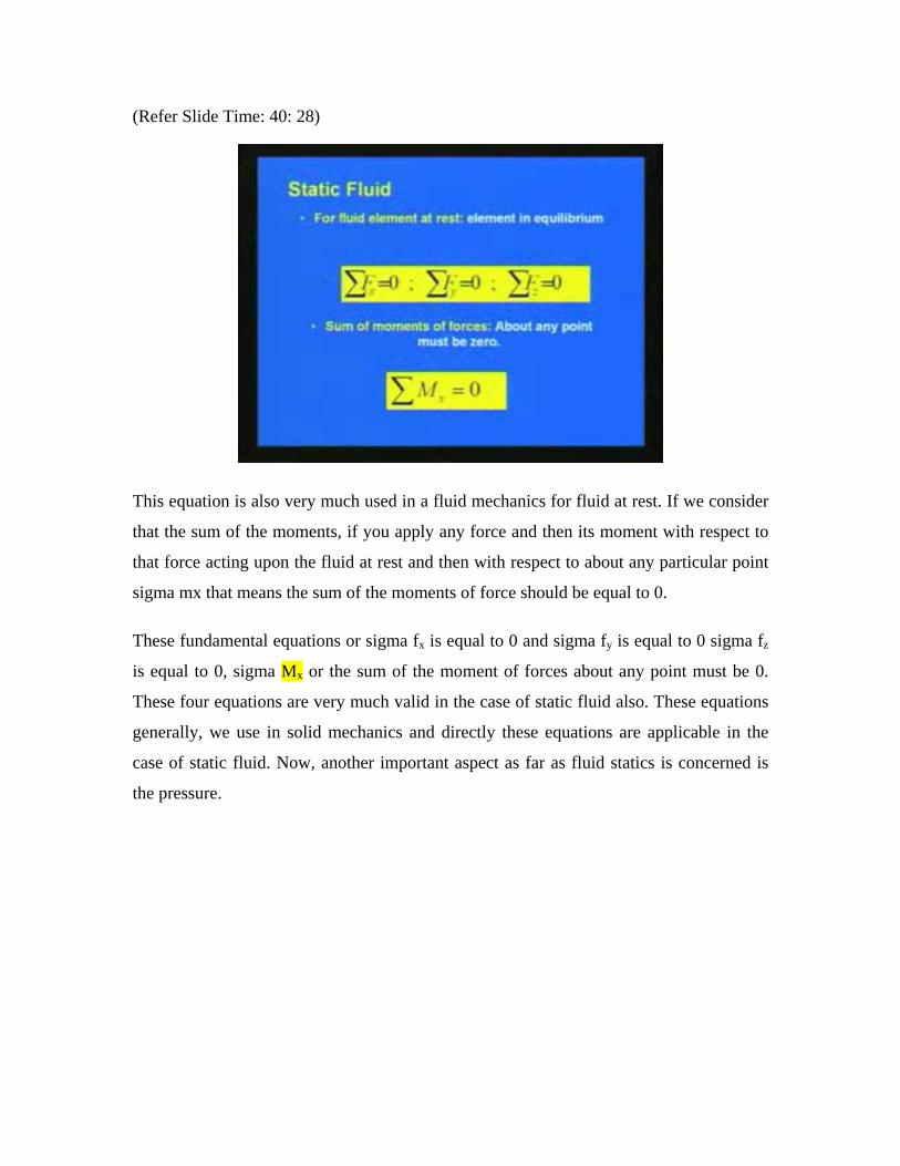
This equation is also very much used in a fluid mechanics for fluid at rest. If we consider
that the sum of the moments, if you apply any force and then its moment with respect to
that force acting upon the fluid at rest and then with respect to about any particular point
sigma mx that means the sum of the moments of force should be equal to 0.
These fundamental equations or sigma fx is equal to 0 and sigma fy is equal to 0 sigma fz
is equal to 0, sigma Mx or the sum of the moment of forces about any point must be 0.
These four equations are very much valid in the case of static fluid also. These equations
generally, we use in solid mechanics and directly these equations are applicable in the
case of static fluid. Now, another important aspect as far as fluid statics is concerned is
the pressure.
(Refer Slide Time: 41:02)
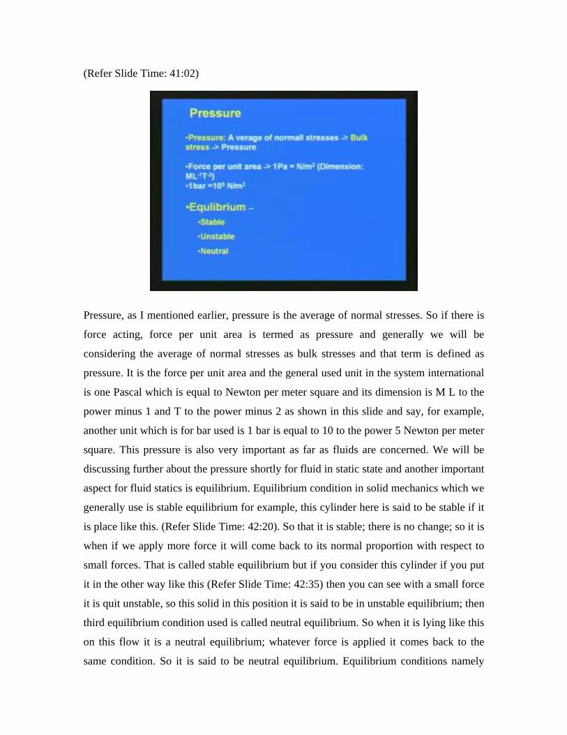
Pressure, as I mentioned earlier, pressure is the average of normal stresses. So if there is
force acting, force per unit area is termed as pressure and generally we will be
considering the average of normal stresses as bulk stresses and that term is defined as
pressure. It is the force per unit area and the general used unit in the system international
is one Pascal which is equal to Newton per meter square and its dimension is M L to the
power minus 1 and T to the power minus 2 as shown in this slide and say, for example,
another unit which is for bar used is 1 bar is equal to 10 to the power 5 Newton per meter
square. This pressure is also very important as far as fluids are concerned. We will be
discussing further about the pressure shortly for fluid in static state and another important
aspect for fluid statics is equilibrium. Equilibrium condition in solid mechanics which we
generally use is stable equilibrium for example, this cylinder here is said to be stable if it
is place like this. (Refer Slide Time: 42:20). So that it is stable; there is no change; so it is
when if we apply more force it will come back to its normal proportion with respect to
small forces. That is called stable equilibrium but if you consider this cylinder if you put
it in the other way like this (Refer Slide Time: 42:35) then you can see with a small force
it is quit unstable, so this solid in this position it is said to be in unstable equilibrium; then
third equilibrium condition used is called neutral equilibrium. So when it is lying like this
on this flow it is a neutral equilibrium; whatever force is applied it comes back to the
same condition. So it is said to be neutral equilibrium. Equilibrium conditions namely
stable equilibrium, unstable equilibrium and neutral equilibrium are very much solid
mechanics. These equilibrium conditions are also very much valid in the case of statics
fluid which will be discussing later.
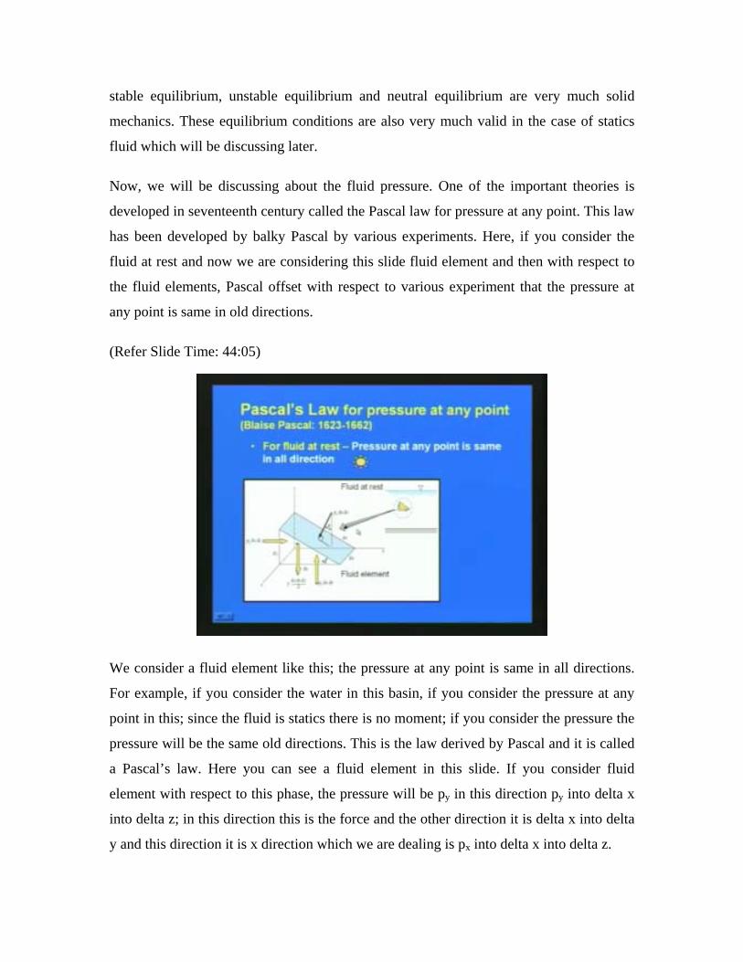
Now, we will be discussing about the fluid pressure. One of the important theories is
developed in seventeenth century called the Pascal law for pressure at any point. This law
has been developed by balky Pascal by various experiments. Here, if you consider the
fluid at rest and now we are considering this slide fluid element and then with respect to
the fluid elements, Pascal offset with respect to various experiment that the pressure at
any point is same in old directions.
(Refer Slide Time: 44:05)
We consider a fluid element like this; the pressure at any point is same in all directions.
For example, if you consider the water in this basin, if you consider the pressure at any
point in this; since the fluid is statics there is no moment; if you consider the pressure the
pressure will be the same old directions. This is the law derived by Pascal and it is called
a Pascal’s law. Here you can see a fluid element in this slide. If you consider fluid
element with respect to this phase, the pressure will be py in this direction py into delta x
into delta z; in this direction this is the force and the other direction it is delta x into delta
y and this direction it is x direction which we are dealing is px into delta x into delta z.
(Refer Slide Time: 45:05)
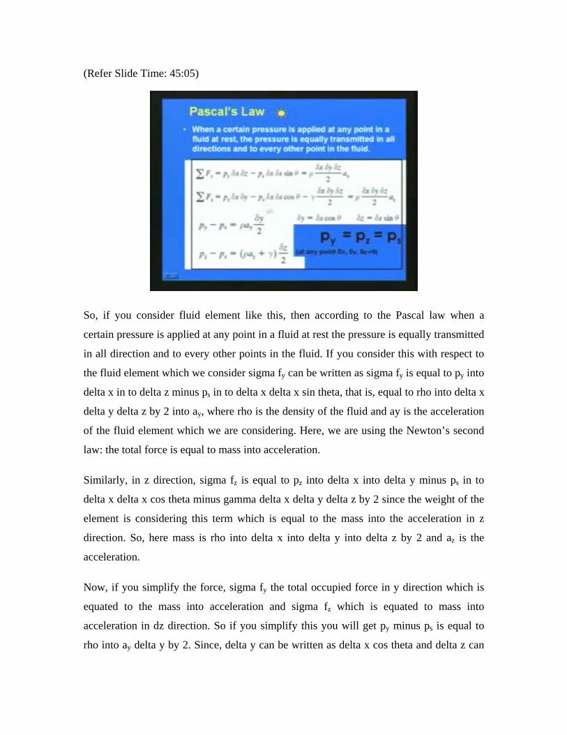
So, if you consider fluid element like this, then according to the Pascal law when a
certain pressure is applied at any point in a fluid at rest the pressure is equally transmitted
in all direction and to every other points in the fluid. If you consider this with respect to
the fluid element which we consider sigma fy can be written as sigma fy is equal to py into
delta x in to delta z minus ps in to delta x delta x sin theta, that is, equal to rho into delta x
delta y delta z by 2 into ay, where rho is the density of the fluid and ay is the acceleration
of the fluid element which we are considering. Here, we are using the Newton’s second
law: the total force is equal to mass into acceleration.
Similarly, in z direction, sigma fz is equal to pz into delta x into delta y minus ps in to
delta x delta x cos theta minus gamma delta x delta y delta z by 2 since the weight of the
element is considering this term which is equal to the mass into the acceleration in z
direction. So, here mass is rho into delta x into delta y into delta z by 2 and az is the
acceleration.
Now, if you simplify the force, sigma fy the total occupied force in y direction which is
equated to the mass into acceleration and sigma fz which is equated to mass into
acceleration in dz direction. So if you simplify this you will get py minus ps is equal to
rho into ay delta y by 2. Since, delta y can be written as delta x cos theta and delta z can
be written as delta x sin theta, the second equation can be written as pz minus ps is equal
to rho into az plus gamma into delta z by 2. Now, with respect to the Pascal law if you
consider the fluid at a particular point then you can see that delta x, delta y and delta z
will be tending to 0. So that we can see py is equal to pz is equal to ps as shown in this
slide. That means the pressure at any particular point is same in all directions. So, here, if
you consider the pressure at particular point at all directions it will be same according to
the Pascal’s law
After discussing the Pascal’s law, we will be discussing the pressure variations at various
vertical direction are shown in a direction and then we trying to derive general equations
which can be applied in all the cases.
(Refer Slide Time: 48:15)
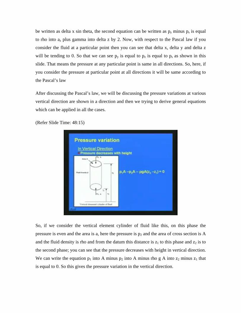
So, if we consider the vertical element cylinder of fluid like this, on this phase the
pressure is even and the area is a, here the pressure is p2 and the area of cross section is A
and the fluid density is rho and from the datum this distance is z1 to this phase and z2 is to
the second phase; you can see that the pressure decreases with height in vertical direction.
We can write the equation p1 into A minus p2 into A minus rho g A into z2 minus z1 that
is equal to 0. So this gives the pressure variation in the vertical direction.
(Refer Slide Time: 48:57)
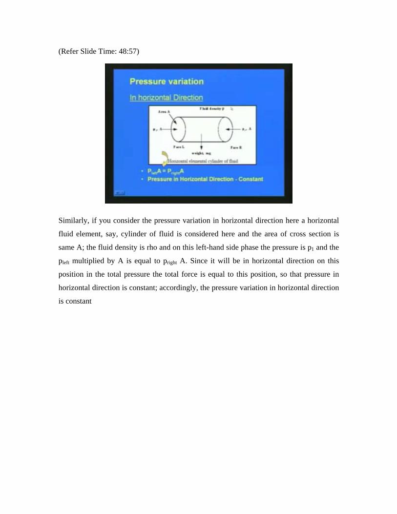
Similarly, if you consider the pressure variation in horizontal direction here a horizontal
fluid element, say, cylinder of fluid is considered here and the area of cross section is
same A; the fluid density is rho and on this left-hand side phase the pressure is p1 and the
pleft multiplied by A is equal to pright A. Since it will be in horizontal direction on this
position in the total pressure the total force is equal to this position, so that pressure in
horizontal direction is constant; accordingly, the pressure variation in horizontal direction
is constant
(Refer Slide Time: 49:49)
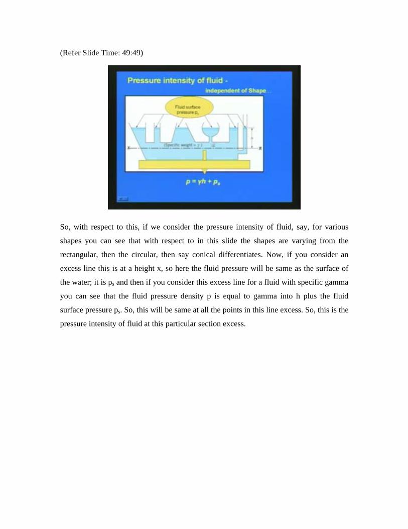
So, with respect to this, if we consider the pressure intensity of fluid, say, for various
shapes you can see that with respect to in this slide the shapes are varying from the
rectangular, then the circular, then say conical differentiates. Now, if you consider an
excess line this is at a height x, so here the fluid pressure will be same as the surface of
the water; it is ps and then if you consider this excess line for a fluid with specific gamma
you can see that the fluid pressure density p is equal to gamma into h plus the fluid
surface pressure ps. So, this will be same at all the points in this line excess. So, this is the
pressure intensity of fluid at this particular section excess.
(Refer Slide Time: 50:37)
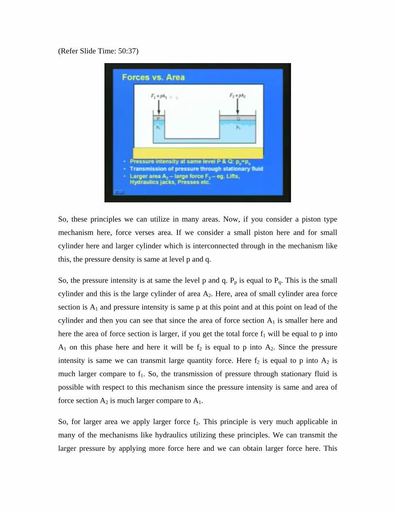
So, these principles we can utilize in many areas. Now, if you consider a piston type
mechanism here, force verses area. If we consider a small piston here and for small
cylinder here and larger cylinder which is interconnected through in the mechanism like
this, the pressure density is same at level p and q.
So, the pressure intensity is at same the level p and q. Pp is equal to Pq. This is the small
cylinder and this is the large cylinder of area A2. Here, area of small cylinder area force
section is A1 and pressure intensity is same p at this point and at this point on lead of the
cylinder and then you can see that since the area of force section A1 is smaller here and
here the area of force section is larger, if you get the total force f1 will be equal to p into
A1 on this phase here and here it will be f2 is equal to p into A2. Since the pressure
intensity is same we can transmit large quantity force. Here f2 is equal to p into A2 is
much larger compare to f1. So, the transmission of pressure through stationary fluid is
possible with respect to this mechanism since the pressure intensity is same and area of
force section A2 is much larger compare to A1.
So, for larger area we apply larger force f2. This principle is very much applicable in
many of the mechanisms like hydraulics utilizing these principles. We can transmit the
larger pressure by applying more force here and we can obtain larger force here. This
principle is used in lifts, hydraulic jacks, pressure extra. What we are doing here is we are
applying a small force here f1 that will give correspondingly large force; input will be
small and larger force output is produced here which is used in lifts hydraulics jacks
pressures and many other hydraulics equipments. So this principle is very much very
important in fluid statics which is based upon the theory that the transmission of pressure
through stationary fluid.
![L-14 Fluids [3] Fluids at rest Fluids at rest Why things float Archimedes’ Principle Fluids in Motion Fluid Dynamics Fluids in Motion Fluid Dynamics.](https://static.fdocuments.in/doc/165x107/56649d845503460f94a6ab30/l-14-fluids-3-fluids-at-rest-fluids-at-rest-why-things-float-archimedes.jpg)


![L-14 Fluids [3] Fluids at rest Fluid Statics Fluids at rest Fluid Statics Why things float Archimedes’ Principle Fluids in Motion Fluid Dynamics.](https://static.fdocuments.in/doc/165x107/56649ced5503460f949ba1d5/l-14-fluids-3-fluids-at-rest-fluid-statics-fluids-at-rest-fluid-statics.jpg)