FLUID MECHANICS LECTURE NOTES
238
1 Chapter1 : Introduction and Fundamental Concepts Lecture 1 : Definition of Stress Consider a small area δA on the surface of a body (Fig. 1.1). The force acting on this area is δF This force can be resolved into two perpendicular components The component of force acting normal to the area called normal force and is denoted by δF n The component of force acting along the plane of area is called tangential force and is denoted by δF t Fig 1.1 Normal and Tangential Forces on a surface When they are expressed as force per unit area they are called as normal stress and tangential stress respectively . The tangential stress is also called shear stress The normal stress (1.1) And shear stress (1.2)
Transcript of FLUID MECHANICS LECTURE NOTES
7/29/2019 FLUID MECHANICS LECTURE NOTES
http://slidepdf.com/reader/full/fluid-mechanics-lecture-notes 1/297
1
Chapter1 : Introduction and Fundamental Concepts
Lecture 1 :
Definition of Stress
Consider a small area δA on the surface of a body (Fig. 1.1). The force acting on thisarea is δF This force can be resolved into two perpendicular components
The component of force acting normal to the area called normal force and is
denoted by δFn The component of force acting along the plane of area is called tangential
force and is denoted by δFt
Fig 1.1 Normal and Tangential Forces on a surface
When they are expressed as force per unit area they are called as normal stress and tangentialstress respectively. The tangential stress is also
called shear stress
The normal stress
(1.1)
And shear stress
(1.2)

7/29/2019 FLUID MECHANICS LECTURE NOTES
http://slidepdf.com/reader/full/fluid-mechanics-lecture-notes 2/297
2
Chapter1 : Introduction and Fundamental Concepts
Lecture 1 :
Definition of Fluid
A fluid is a substance that deforms continuously in the face of tangential or shear stress, irrespective of the magnitude of shear stress .This continuousdeformation under the application of shear stress constitutes a flow.
In this connection fluid can also be defined as the state of matter that cannotsustain any shear stress.
Example : Consider Fig 1.2
Fig 1.2 Shear stress on a fluid body
If a shear stress τ is applied at any location in a fluid, the element 011' which is initiallyat rest, will move to 022', then to 033'. Further, it moves to 044' and continues to movein a similar fashion.
In other words, the tangential stress in a fluid body depends on velocity ofdeformation and vanishes as this velocity approaches zero. A good example is Newton's parallel plate experiment where dependence of shear force on the velocityof deformation was established.
Chapter 1 : Introduction and Fundamental Concepts
Lecture 1 :
7/29/2019 FLUID MECHANICS LECTURE NOTES
http://slidepdf.com/reader/full/fluid-mechanics-lecture-notes 3/297
3
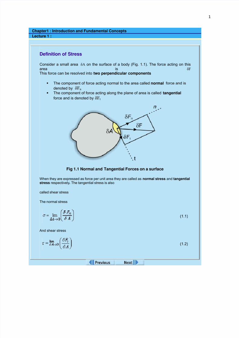
Distinction Between Solid and Fluid
Solid Fluid
More Compact Structure
Attractive Forces between the moleculesare larger therefore more closely packed
Solids can resist tangential stresses instatic condition
Whenever a solid is subjected to shear stress
a. It undergoes a definite
deformation α or breaks
b. α is proportional to shear stress
upto some limiting condition
Solid may regain partly or fully itsoriginal shape when the tangentialstress is removed
Less Compact Structure
Attractive Forces between the moleculesare smaller therefore more looselypacked
Fluids cannot resist tangential stresses instatic condition.
Whenever a fluid is subjected to shear stress
a. No fixed deformation
b. Continious deformation takesplaceuntil the shear stress is applied
A fluid can never regain its originalshape, once it has been distorded by theshear stress
Fig 1.3 Deformation of a Solid Body
Chapter1 : Introduction and Fundamental Concepts
Lecture 1 :
7/29/2019 FLUID MECHANICS LECTURE NOTES
http://slidepdf.com/reader/full/fluid-mechanics-lecture-notes 4/297
4
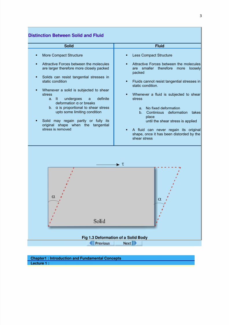
Concept of Continuum
The concept of continuum is a kind of idealization of the continuous description of matter where the properties of the matter are considered as continuous functions of space variables. Although any matter is composed of several molecules, the conceptof continuum assumes a continuous distribution of mass within the matter or systemwith no empty space, instead of the actual conglomeration of separate molecules.
Describing a fluid flow quantitatively makes it necessary to assume that flowvariables (pressure , velocity etc.) and fluid properties vary continuously from onepoint to another. Mathematical description of flow on this basis have proved to bereliable and treatment of fluid medium as a continuum has firmly becomeestablished. For example density at a point is normally defined as
Here Δ is the volume of the fluid element and m is the mass
If Δ is very large ρ is affected by the inhomogeneities in the fluid medium.Considering another extreme if Δ is very small, random movement of atoms (or molecules) would change their number at different times. In the continuumapproximation point density is defined at the smallest magnitude of Δ , beforestatistical fluctuations become significant. This is called continuum limit and isdenoted by Δ c.
Chapter1 : Introduction and Fundamental Concepts
Lecture 1 :
7/29/2019 FLUID MECHANICS LECTURE NOTES
http://slidepdf.com/reader/full/fluid-mechanics-lecture-notes 5/297
5
Concept of Continuum - contd from previous slide
One of the factors considered important in determining the validity of continuum model is molecular density. It is the distance between the
molecules which is characterised by mean free path ( λ ). It iscalculated by finding statistical average distance the molecules travelbetween two successive collisions. If the mean free path is very smallas compared with some characteristic length in the flow domain (i.e.,the molecular density is very high) then the gas can be treated as acontinuous medium. If the mean free path is large in comparison tosome characteristic length, the gas cannot be considered continuousand it should be analysed by the molecular theory.
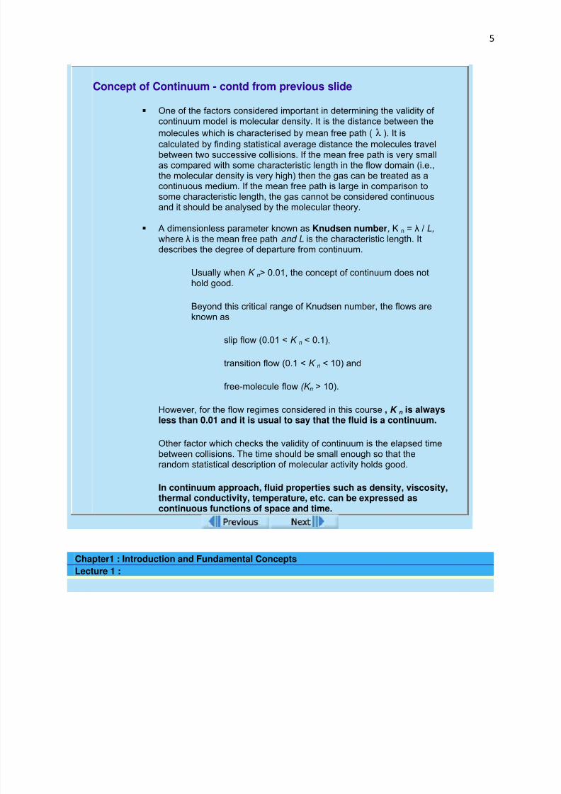
A dimensionless parameter known as Knudsen number, K n = λ / L,where λ is the mean free path and L is the characteristic length. Itdescribes the degree of departure from continuum.
Usually when K n > 0.01, the concept of continuum does not
hold good.
Beyond this critical range of Knudsen number, the flows areknown as
slip flow (0.01 < K n < 0.1),
transition flow (0.1 < K n < 10) and
free-molecule flow (K n > 10).
However, for the flow regimes considered in this course , K n is always
less than 0.01 and it is usual to say that the fluid is a continuum.
Other factor which checks the validity of continuum is the elapsed timebetween collisions. The time should be small enough so that therandom statistical description of molecular activity holds good.
In continuum approach, fluid properties such as density, viscosity,thermal conductivity, temperature, etc. can be expressed ascontinuous functions of space and time.
Chapter1 : Introduction and Fundamental ConceptsLecture 1 :
7/29/2019 FLUID MECHANICS LECTURE NOTES
http://slidepdf.com/reader/full/fluid-mechanics-lecture-notes 6/297
6
Fluid Properties :
Characteristics of a continuous fluid which are independent of the motion of the fluid are called basicproperties of the fluid. Some of the basic properties are as discussed below.
perty Symbol Definition U
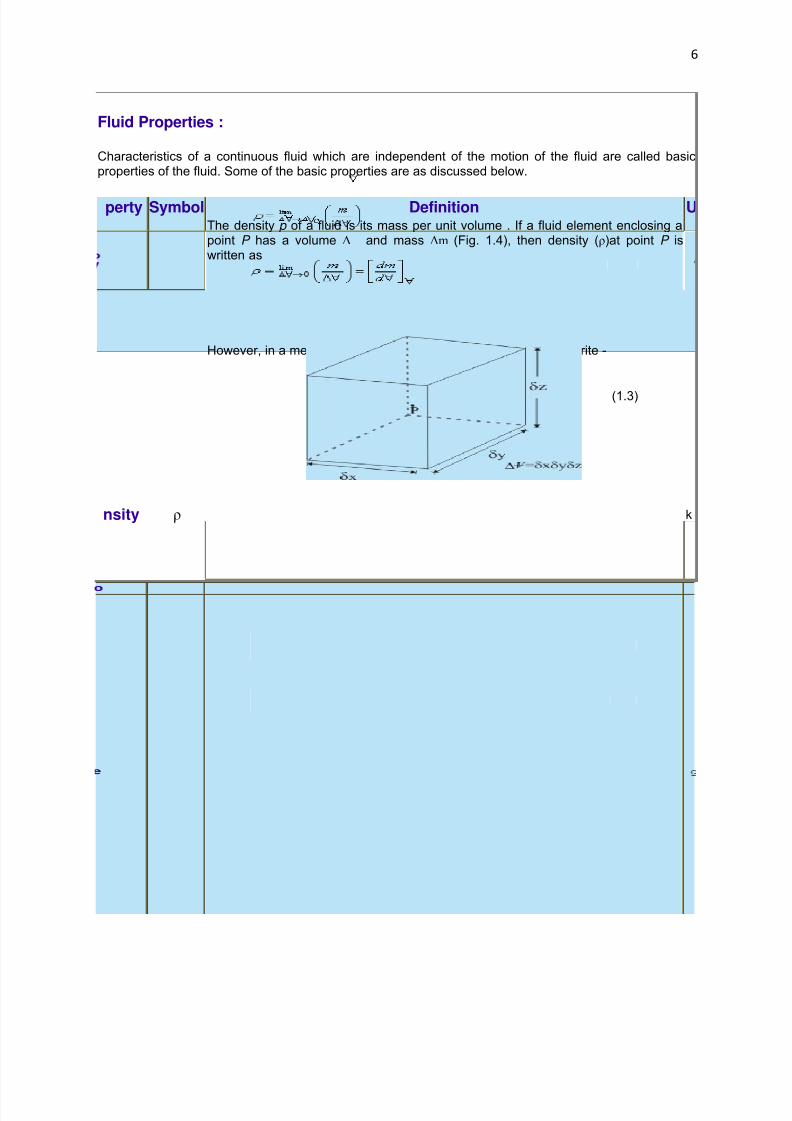
nsity ρ
The density p of a fluid is its mass per unit volume . If a fluid element enclosing apoint P has a volume Δ and mass Δm (Fig. 1.4), then density (ρ)at point P iswritten as
However, in a medium where continuum model is valid one can write -
(1.3)
Fig 1.4 A fluid element enclosing point P
k
ecificeight
γ
The specific weight is the weight of fluid per unit volume. The specific weight isgiven
by γ= ρg (1.4)
Where g is the gravitational acceleration. Just as weight must be clearly
N
7/29/2019 FLUID MECHANICS LECTURE NOTES
http://slidepdf.com/reader/full/fluid-mechanics-lecture-notes 7/297
7
distinguished from mass, so must the specific weight be distinguished from density.
Specific
Volume
v
The specific volume of a fluid is the volume occupied by unit mass of fluid.
Thus
(1.5)
m3
/kg
SpecificGravity
s
For liquids, it is the ratio of density of a liquid at actual conditions to the density of pure water at 101 kN/m
2, and at 4°C.
The specific gravity of a gas is the ratio of its density to that of either hydrogen or air at some specified temperature or pressure.
However, there is no general standard; so the conditions must be statedwhile referring to the specific gravity of a gas.
-
Chapter1 : Introduction and Fundamental Concepts
Lecture 1 :
Viscosity ( μ ) :
Viscosity is a fluid property whose effect is understood when the fluid is in motion. In a flow of fluid, when the fluid elements move with different velocities, each element will feel
some resistance due to fluid friction within the elements. Therefore, shear stresses can be identified between the fluid elements with different
velocities. The relationship between the shear stress and the velocity field was given by Sir Isaac
Newton.
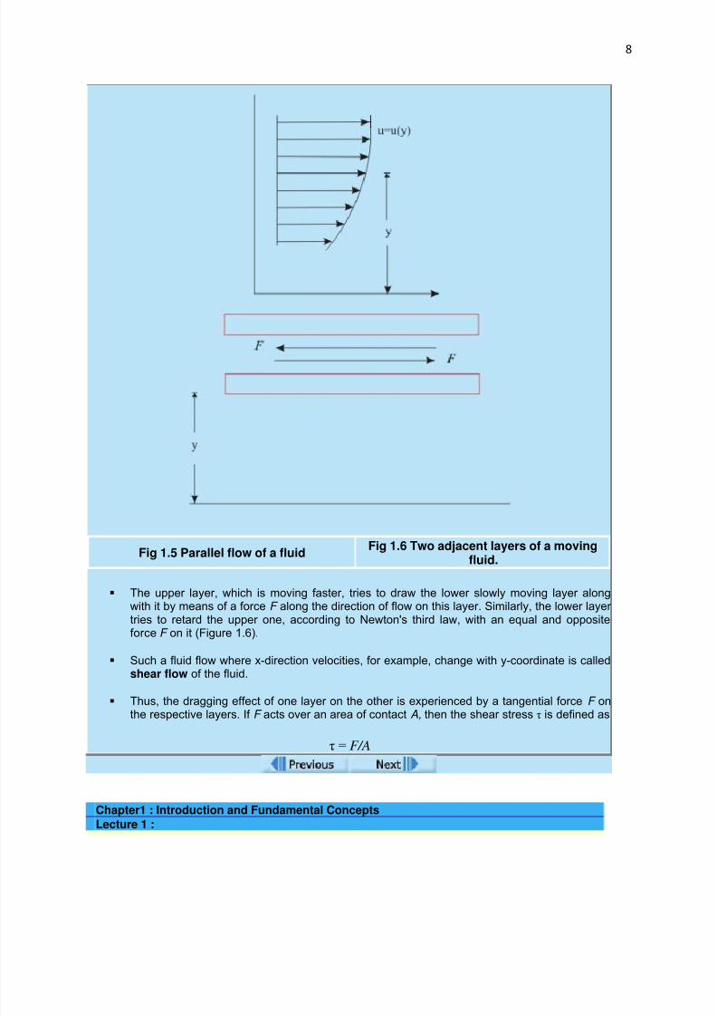
Consider a flow (Fig. 1.5) in which all fluid particles are moving in the same direction in such a waythat the fluid layers move parallel with different velocities.
7/29/2019 FLUID MECHANICS LECTURE NOTES
http://slidepdf.com/reader/full/fluid-mechanics-lecture-notes 8/297
8
Fig 1.5 Parallel flow of a fluidFig 1.6 Two adjacent layers of a moving
fluid.
The upper layer, which is moving faster, tries to draw the lower slowly moving layer alongwith it by means of a force F along the direction of flow on this layer. Similarly, the lower layer tries to retard the upper one, according to Newton's third law, with an equal and oppositeforce F on it (Figure 1.6).
Such a fluid flow where x-direction velocities, for example, change with y-coordinate is calledshear flow of the fluid.
Thus, the dragging effect of one layer on the other is experienced by a tangential force F on
the respective layers. If F acts over an area of contact A, then the shear stress τ is defined as
τ = F/A
Chapter1 : Introduction and Fundamental Concepts
Lecture 1 :

7/29/2019 FLUID MECHANICS LECTURE NOTES
http://slidepdf.com/reader/full/fluid-mechanics-lecture-notes 9/297
9
Viscosity ( μ ) :
Newton postulated that τ is proportional to the quantity Δu/ Δy where Δy is thedistance of separation of the two layers and Δu is the difference in their velocities.
In the limiting case of , Δu / Δy equals du/dy, the velocity gradient at a point in adirection perpendicular to the direction of the motion of the layer.
According to Newton τ and du/dy bears the relation
(1.7)
where, the constant of proportionality μ is known as the coefficient of viscosity or simply
viscosity which is a property of the fluid and depends on its state. Sign of τ depends upon
the sign of du/dy. For the profile shown in Fig. 1.5, du/dy is positive everywhere and hence, τis positive. Both the velocity and stress are considered positive in the positive direction of thecoordinate parallel to them.Equation
defining the viscosity of a fluid, is known as Newton's law of viscosity. Common fluids, viz.water, air, mercury obey Newton's law of viscosity and are known as Newtonian fluids.
Other classes of fluids, viz. paints, different polymer solution, blood do not obey the typical
linear relationship, of τ and du/dy and are known as non-Newtonian fluids. In non-newtonian fluids viscosity itself may be a function of deformation rate as you will study in thenext lecture.
Chapter1 : Introduction and Fundamental Concepts
Lecture 1 :

7/29/2019 FLUID MECHANICS LECTURE NOTES
http://slidepdf.com/reader/full/fluid-mechanics-lecture-notes 10/297
10
Causes of Viscosity - contd from previous slide...
As the random molecular motion increases with a rise in temperature, the viscosityalso increases accordingly. Except for very special cases (e.g., at very highpressure) the viscosity of both liquids and gases ceases to be a function of pressure.
For Newtonian fluids, the coefficient of viscosity depends strongly on temperaturebut varies very little with pressure.
For liquids, molecular motion is less significant than the forces of cohesion, thus viscosity of liquids decrease with increase in temperature.
For gases,molecular motion is more significant than the cohesive forces, thus viscosity of gases increase with increase in temperature.
Fig 1.8: Change of Viscosity of Water and Air under 1 atm
No-slip Condition of Viscous Fluids
It has been established through experimental observations that the relative velocitybetween the solid surface and the adjacent fluid particles is zero whenever a viscousfluid flows over a solid surface. This is known as no-slip condition.
This behavior of no-slip at the solid surface is not same as the wetting of surfaces bythe fluids. For example, mercury flowing in a stationary glass tube will not wet the

7/29/2019 FLUID MECHANICS LECTURE NOTES
http://slidepdf.com/reader/full/fluid-mechanics-lecture-notes 11/297
11
surface, but will have zero velocity at the wall of the tube.
The wetting property results from surface tension, whereas the no-slip condition is aconsequence of fluid viscosity.
End of Lecture 1!
To start next lecture click next buttonor select from left-hand-side.
Chapter1 : Introduction and Fundamental Concepts
Lecture 2 :
Ideal Fluid
Consider a hypothetical fluid having a zero viscosity ( μ = 0). Such a fluid iscalled an ideal fluid and the resulting motion is called as ideal or inviscid flow.In an ideal flow, there is no existence of shear force because of vanishingviscosity.
All the fluids in reality have viscosity ( μ > 0) and hence they are termed asreal fluid and their motion is known as viscous flow.
Under certain situations of very high velocity flow of viscous fluids, an accurateanalysis of flow field away from a solid surface can be made from the ideal flowtheory.
Non-Newtonian Fluids
There are certain fluids where the linear relationship between the shear stressand the deformation rate (velocity gradient in parallel flow) as expressed by the
is not valid. For these fluids the viscosity varies with rate of

7/29/2019 FLUID MECHANICS LECTURE NOTES
http://slidepdf.com/reader/full/fluid-mechanics-lecture-notes 12/297
12
deformation.
Due to the deviation from Newton's law of viscosity they are commonly termed
as non-Newtonian fluids. Figure 2.1 shows the class of fluid for which thisrelationship is nonlinear.
Figure 2.1 Shear stress and deformation rate relationship of different fluids
The abscissa in Fig. 2.1 represents the behaviour of ideal fluids since for theideal fluids the resistance to shearing deformation rate is always zero, andhence they exhibit zero shear stress under any condition of flow.
The ordinate represents the ideal solid for there is no deformation rate under any loading condition.
The Newtonian fluids behave according to the law that shear stress is linearly
proportional to velocity gradient or rate of shear strain . Thus for these fluids, the plot of shear stress against velocity gradient is a straight linethrough the origin. The slope of the line determines the viscosity.
The non-Newtonian fluids are further classified as pseudo-plastic, dilatant and
Bingham plastic.
Chapter1 : Introduction and Fundamental Concepts
Lecture 2 :

7/29/2019 FLUID MECHANICS LECTURE NOTES
http://slidepdf.com/reader/full/fluid-mechanics-lecture-notes 13/297
13
Compressibility
Compressibility of any substance is the measure of its change in volume under theaction of external forces.
The normal compressive stress on any fluid element at rest is known as hydrostaticpressure p and arises as a result of innumerable molecular collisions in the entirefluid.
The degree of compressibility of a substance is characterized by the bulk modulusof elasticity E defined as
(2.3)
Wher e Δ and Δp are the changes in the volume and pressure respectively, and is
the initial volume. The negative sign (-sign) is included to make E positive, sinceincrease in pressure would decrease the volume i.e for Δp>0 , Δ <0) in volume.
For a given mass of a substance, the change in its volume and density satisfies therelation
m = 0, ρ ) = 0
(2.4)
using
we get
(2.5)
Values of E for liquids are very high as compared with those of gases (except at veryhigh pressures). Therefore, liquids are usually termed as incompressible fluids
though, in fact, no substance is theoretically incompressible with a value of E as .
For example, the bulk modulus of elasticity for water and air at atmospheric pressureare approximately 2 x 10
6kN/m
2and 101 kN/m
2respectively. It indicates that air is
about 20,000 times more compressible than water. Hence water can be treated asincompressible.
7/29/2019 FLUID MECHANICS LECTURE NOTES
http://slidepdf.com/reader/full/fluid-mechanics-lecture-notes 14/297
14
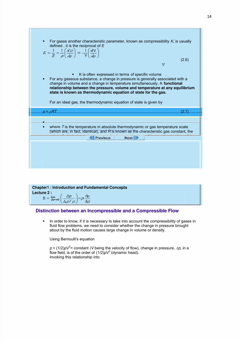
For gases another characteristic parameter, known as compressibility K, is usuallydefined , it is the reciprocal of E
(2.6)
K is often expressed in terms of specific volume . For any gaseous substance, a change in pressure is generally associated with a
change in volume and a change in temperature simultaneously. A functionalrelationship between the pressure, volume and temperature at any equilibriumstate is known as thermodynamic equation of state for the gas.
For an ideal gas, the thermodynamic equation of state is given by
p = ρRT (2.7)
where T is the temperature in absolute thermodynamic or gas temperature scale(which are, in fact, identical), and R is known as the characteristic gas constant, thevalue of which depends upon a particular gas. However, this equation is also validfor the real gases which are thermodynamically far from their liquid phase. For air,the value of R is 287 J/kg K.
K and E generally depend on the nature of process
Chapter1 : Introduction and Fundamental Concepts
Lecture 2 :
Distinction between an Incompressible and a Compressible Flow
In order to know, if it is necessary to take into account the compressibility of gases influid flow problems, we need to consider whether the change in pressure broughtabout by the fluid motion causes large change in volume or density.
Using Bernoulli's equation
p + (1/2)ρV2= constant (V being the velocity of flow), change in pressure, Δp, in a
flow field, is of the order of (1/2)ρV2(dynamic head).
Invoking this relationship into

7/29/2019 FLUID MECHANICS LECTURE NOTES
http://slidepdf.com/reader/full/fluid-mechanics-lecture-notes 15/297
15
we get ,
(2.12)
So if Δρ/ρ is very small, the flow of gases can be treated as incompressiblewith a good degree of approximation.
According to Laplace's equation, the velocity of sound is given by
Hence
where, Ma is the ratio of the velocity of flow to the acoustic velocity in the flowingmedium at the condition and is known as Mach number. So we can conclude thatthe compressibility of gas in a flow can be neglected if Δρ/ρ is considerably smaller than unity, i.e. (1/2)Ma
2<<1.
In other words, if the flow velocity is small as compared to the local acoustic velocity,compressibility of gases can be neglected. Considering a maximum relative
change in density of 5 per cent as the criterion of an incompressible flow, theupper limit of Mach number becomes approximately 0.33. In the case of air atstandard pressure and temperature, the acoustic velocity is about 335.28 m/s.Hence a Mach number of 0.33 corresponds to a velocity of about 110 m/s. Thereforeflow of air up to a velocity of 110 m/s under standard condition can be considered asincompressible flow.
Chapter1 : Introduction and Fundamental ConceptsLecture 2 :
7/29/2019 FLUID MECHANICS LECTURE NOTES
http://slidepdf.com/reader/full/fluid-mechanics-lecture-notes 16/297
16
Surface Tension of Liquids
The phenomenon of surface tension arises due to the two kinds of intermolecular forces
(i) Cohesion : The force of attraction between the molecules of a liquid byvirtue of which they are bound to each other to remain as one assemblage of particles is known as the force of cohesion. This property enables the liquid toresist tensile stress.
(ii) Adhesion : The force of attraction between unlike molecules, i.e. betweenthe molecules of different liquids or between the molecules of a liquid and thoseof a solid body when they are in contact with each other, is known as the forceof adhesion. This force enables two different liquids to adhere to each other or aliquid to adhere to a solid body or surface.
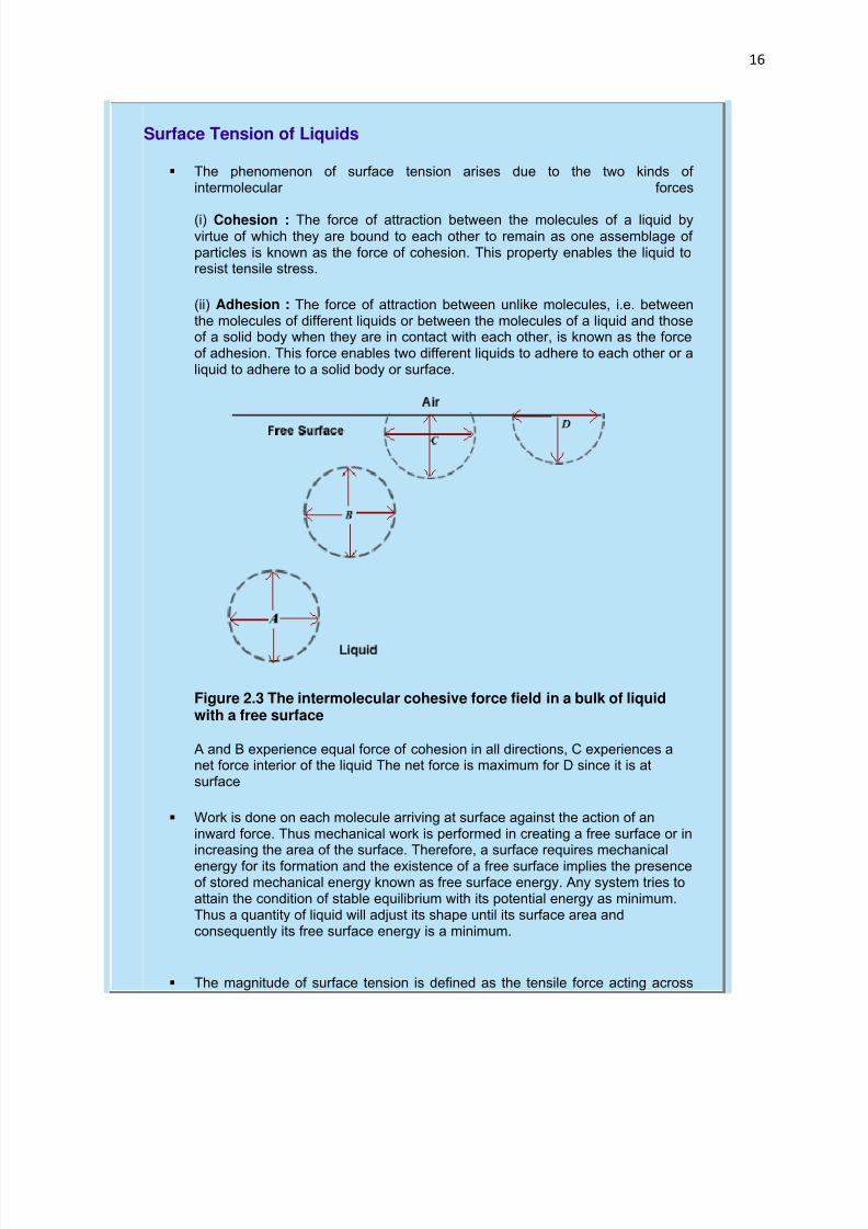
Figure 2.3 The intermolecular cohesive force field in a bulk of liquidwith a free surface
A and B experience equal force of cohesion in all directions, C experiences anet force interior of the liquid The net force is maximum for D since it is atsurface
Work is done on each molecule arriving at surface against the action of aninward force. Thus mechanical work is performed in creating a free surface or inincreasing the area of the surface. Therefore, a surface requires mechanical
energy for its formation and the existence of a free surface implies the presenceof stored mechanical energy known as free surface energy. Any system tries toattain the condition of stable equilibrium with its potential energy as minimum.Thus a quantity of liquid will adjust its shape until its surface area andconsequently its free surface energy is a minimum.
The magnitude of surface tension is defined as the tensile force acting across

7/29/2019 FLUID MECHANICS LECTURE NOTES
http://slidepdf.com/reader/full/fluid-mechanics-lecture-notes 17/297
17
imaginary short and straight elemental line divided by the length of the line.
The dimensional formula is F/L or MT-2
. It is usually expressed in N/m in SIunits.
Surface tension is a binary property of the liquid and gas or two liquids which
are in contact with each other and defines the interface. It decreases slightlywith increasing temperature. The surface tension of water in contact with air at20°C is about 0.073 N/m.
It is due to surface tension that a curved liquid interface in equilibrium results ina greater pressure at the concave side of the surface than that at its convexside.
Chapter1 : Introduction and Fundamental Concepts
Lecture 2 :
Capillarity
The interplay of the forces of cohesion and adhesion explains the phenomenonof capillarity. When a liquid is in contact with a solid, if the forces of adhesionbetween the molecules of the liquid and the solid are greater than the forces of cohesion among the liquid molecules themselves, the liquid molecules crowdtowards the solid surface. The area of contact between the liquid and solidincreases and the liquid thus wets the solid surface.
The reverse phenomenon takes place when the force of cohesion is greater than the force of adhesion. These adhesion and cohesion properties result inthe phenomenon of capillarity by which a liquid either rises or falls in a tubedipped into the liquid depending upon whether the force of adhesion is morethan that of cohesion or not (Fig.2.4).
The angle θ as shown in Fig. 2.4, is the area wetting contact angle made by theinterface with the solid surface.

7/29/2019 FLUID MECHANICS LECTURE NOTES
http://slidepdf.com/reader/full/fluid-mechanics-lecture-notes 18/297
18
Fig 2.4 Phenomenon of Capillarity
For pure water in contact with air in a clean glass tube, the capillary rise takesplace with θ = 0 . Mercury causes capillary depression with an angle of contactof about 130
0in a clean glass in contact with air. Since h varies inversely with D
as found from Eq. ( ), an appreciable capillary rise or depressionis observed in tubes of small diameter only.
Chapter1 : Introduction and Fundamental Concepts
Lecture 2 :
Vapour pressure
All l iquids have a tendency to evaporate when exposed to a gaseous atmosphere. Therate of evaporation depends upon the molecular energy of the liquid which in turn
depends upon the type of liquid and its temperature. The vapour molecules exert apartial pressure in the space above the liquid, known as vapour pressure. If the spaceabove the liquid is confined (Fig. 2.5) and the liquid is maintained at constanttemperature, after sufficient time, the confined space above the liquid will containvapour molecules to the extent that some of them will be forced to enter the liquid.Eventually an equilibrium condition will evolve when the rate at which the number of vapour molecules striking back the liquid surface and condensing is just equal to therate at which they leave from the surface. The space above the liquid then becomessaturated with vapour. The vapour pressure of a given liquid is a function of temperature

7/29/2019 FLUID MECHANICS LECTURE NOTES
http://slidepdf.com/reader/full/fluid-mechanics-lecture-notes 19/297
19
only and is equal to the saturation pressure for boiling corresponding to thattemperature. Hence, the vapour pressure increases with the increase in temperature.Therefore the phenomenon of boiling of a liquid is closely related to the vapour pressure. In fact, when the vapour pressure of a liquid becomes equal to the totalpressure impressed on its surface, the liquid starts boiling. This concludes that boilingcan be achieved either by raising the temperature of the liquid, so that its vapour
pressure is elevated to the ambient pressure, or by lowering the pressure of theambience (surrounding gas) to the liquid's vapour pressure at the existing temperature.
Figure 2.5 To and fro movement of liquid molecules from an interface in aconfined space as a closed surrounding
End of Lecture 2!
To view the exercise problem, clicknext button or select from left-hand-side.

7/29/2019 FLUID MECHANICS LECTURE NOTES
http://slidepdf.com/reader/full/fluid-mechanics-lecture-notes 20/297
20
Module 1 :
Chapter 2 : Fluid Statics
The chapter contains
Lecture 3
Forces on Fluid Elements
Normal Stresses in a Stationary Fluid
Fundamental Equation of Fluid Statics
Lecture 4
Units and Scales of Pressure Measurement
Lecture 5
Hydrostatic Thrusts on Submerged Surfaces
Stability of Unconstrained Bodies in Fluid
Period of Oscillation
Exercise Problem

7/29/2019 FLUID MECHANICS LECTURE NOTES
http://slidepdf.com/reader/full/fluid-mechanics-lecture-notes 21/297
21
Chapter2 : Fluid Statics
Lecture 3 :
Forces on Fluid Elements
Fluid Elements - Definition:
Fluid element can be defined as an infinitesimal region of the fluid continuum in isolationfrom its surroundings.
Two types of forces exist on fluid elements
Body Force: distributed over the entire mass or volume of the element. It isusually expressed per unit mass of the element or medium upon which theforces act.Example: Gravitational Force, Electromagnetic force fields etc.
Surface Force: Forces exerted on the fluid element by its surroundings throughdirect contact at the surface.
Surface force has two components: Normal Force: along the normal to the area Shear Force: along the plane of the area.
The ratios of these forces and the elemental area in the limit of the area tending to zeroare called the normal and shear stresses respectively.
The shear force is zero for any fluid element at rest and hence the only surface force ona fluid element is the normal component.
Chapter2 : Fluid Statics
Lecture 3 :
7/29/2019 FLUID MECHANICS LECTURE NOTES
http://slidepdf.com/reader/full/fluid-mechanics-lecture-notes 22/297
22
Normal Stress in a Stationary Fluid
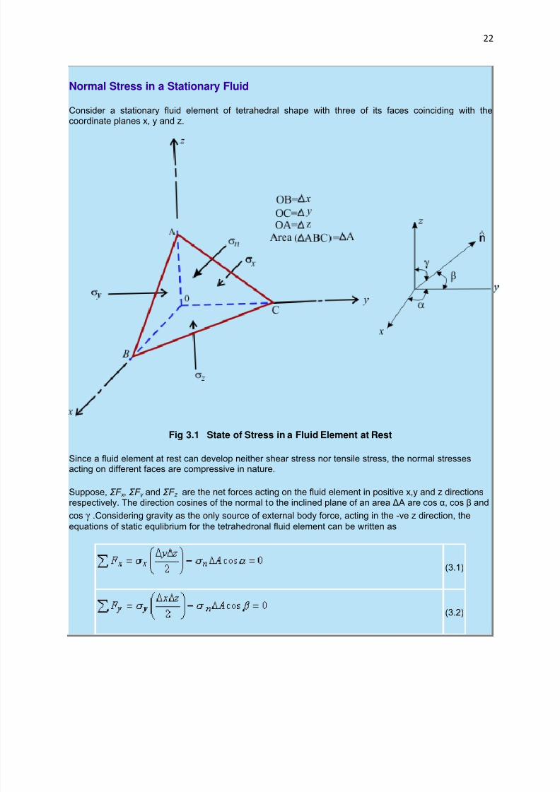
Consider a stationary fluid element of tetrahedral shape with three of its faces coinciding with thecoordinate planes x, y and z.
Fig 3.1 State of Stress in a Fluid Element at Rest
Since a fluid element at rest can develop neither shear stress nor tensile stress, the normal stressesacting on different faces are compressive in nature.
Suppose, ΣF x , ΣF y and ΣF z are the net forces acting on the fluid element in positive x,y and z directionsrespectively. The direction cosines of the normal to the inclined plane of an area ΔA are cos α, cos β and
cos .Considering gravity as the only source of external body force, acting in the -ve z direction, the
equations of static equlibrium for the tetrahedronal fluid element can be written as
(3.1)
(3.2)

7/29/2019 FLUID MECHANICS LECTURE NOTES
http://slidepdf.com/reader/full/fluid-mechanics-lecture-notes 23/297
23
(3.3)
where = Volume of tetrahedral fluid element
Chapter2 : Fluid Statics
Lecture 3 :
Pascal's Law of Hydrostatics
Pascal's Law
The normal stresses at any point in a fluid element at rest are directed towards the pointfrom all directions and they are of the equal magnitude.
Fig 3.2 State of normal stress at a point in a fluid body at rest
Derivation:

7/29/2019 FLUID MECHANICS LECTURE NOTES
http://slidepdf.com/reader/full/fluid-mechanics-lecture-notes 24/297
24
The inclined plane area is related to the fluid elements (refer to Fig 3.1) as follows
(3.4)
(3.5)
(3.6)
Substituting above values in equation 3.1- 3.3 we get
(3.7)
Conclusion:
The state of normal stress at any point in a fluid element at rest is same and directedtowards the point from all directions. These stresses are denoted by a scalar quantity pdefined as the hydrostatic or thermodynamic pressure.Using "+" sign for the tensile stress the above equation can be written in terms of pressure as
(3.8)
Chapter2 : Fluid Statics
Lecture 3 :
7/29/2019 FLUID MECHANICS LECTURE NOTES
http://slidepdf.com/reader/full/fluid-mechanics-lecture-notes 25/297
25
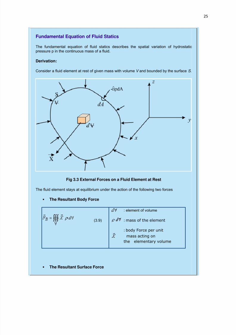
Fundamental Equation of Fluid Statics
The fundamental equation of fluid statics describes the spatial variation of hydrostaticpressure p in the continuous mass of a fluid.
Derivation:
Consider a fluid element at rest of given mass with volume V and bounded by the surface S .
Fig 3.3 External Forces on a Fluid Element at Rest
The fluid element stays at equilibrium under the action of the following two forces
The Resultant Body Force
(3.9)
: element of volume
: mass of the element
: body Force per unit
mass acting on
the elementary volume
The Resultant Surface Force

7/29/2019 FLUID MECHANICS LECTURE NOTES
http://slidepdf.com/reader/full/fluid-mechanics-lecture-notes 26/297
26
(3.10)
dA : area of an element of surface
: the unit vector normal to
the elemental surface,taken positive when directed
outwards
Using Gauss divergence theorem, Eq (3.10) can be written as
(3.11)
Click here to see the derivation
For the fluid element to be in equilibrium , we have
(3.12)
The equation is valid for any volume of the fluid element, no matter how small, thus we get
(3.13)
This is the fundamental equation of fluid statics.
Chapter2 : Fluid Statics
Lecture 3 :
7/29/2019 FLUID MECHANICS LECTURE NOTES
http://slidepdf.com/reader/full/fluid-mechanics-lecture-notes 27/297
27
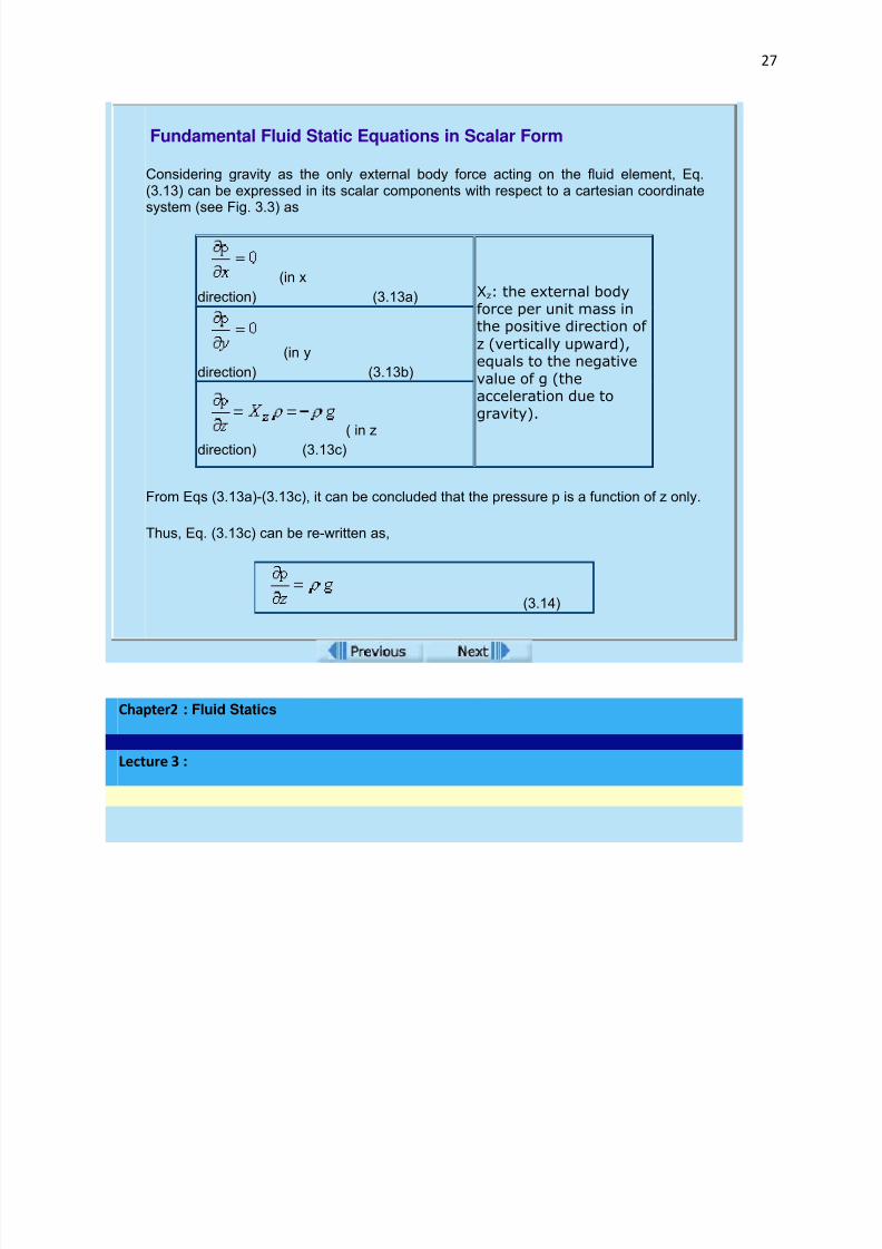
Fundamental Fluid Static Equations in Scalar Form
Considering gravity as the only external body force acting on the fluid element, Eq.(3.13) can be expressed in its scalar components with respect to a cartesian coordinatesystem (see Fig. 3.3) as
(in x
direction) (3.13a) Xz: the external bodyforce per unit mass inthe positive direction of
z (vertically upward),equals to the negative
value of g (theacceleration due to
gravity).
(in y
direction) (3.13b)
( in zdirection) (3.13c)
From Eqs (3.13a)-(3.13c), it can be concluded that the pressure p is a function of z only.
Thus, Eq. (3.13c) can be re-written as,
(3.14)
Chapter2 : Fluid Statics
Lecture 3 :
7/29/2019 FLUID MECHANICS LECTURE NOTES
http://slidepdf.com/reader/full/fluid-mechanics-lecture-notes 28/297
28
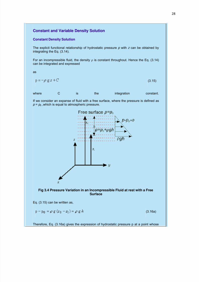
Constant and Variable Density Solution
Constant Density Solution
The explicit functional relationship of hydrostatic pressure p with z can be obtained byintegrating the Eq. (3.14).
For an incompressible fluid, the density is constant throughout. Hence the Eq. (3.14)can be integrated and expressed
as
(3.15)
where C is the integration constant.
If we consider an expanse of fluid with a free surface, where the pressure is defined asp = p 0 ,which is equal to atmospheric pressure.
Fig 3.4 Pressure Variation in an Incompressible Fluid at rest with a FreeSurface
Eq. (3.15) can be written as,
(3.16a)
Therefore, Eq. (3.16a) gives the expression of hydrostatic pressure p at a point whose
7/29/2019 FLUID MECHANICS LECTURE NOTES
http://slidepdf.com/reader/full/fluid-mechanics-lecture-notes 29/297
29
vertical depression from the free surface is h.
Similarly,
(3.16b)
Thus, the difference in pressure between two points in an incompressible fluid at restcan be expressed in terms of the vertical distance between the points. This result isknown as Torricelli's principle, which is the basis for differential pressure measuring`devices. The pressure p0 at free surface is the local atmospheric pressure.
Therefore, it can be stated from Eq. (3.16a), that the pressure at any point in anexpanse of a fluid at rest, with a free surface exceeds that of the local atmosphere by
an amount gh , where h is the vertical depth of the point from the free surface.
Variable Density Solution: As a more generalised case, for compressible fluids at rest,the pressure variation at rest depends on how the fluid density changes with height z
and pressure p. For example this can be done for special cases of "isothermal and non-isothermal fluids"
End of Lecture 3!
To start next lecture click next
button or select from left-hand-
side.
Chapter 2 : Fluid Statics
Lecture 4 :

7/29/2019 FLUID MECHANICS LECTURE NOTES
http://slidepdf.com/reader/full/fluid-mechanics-lecture-notes 30/297
30
Piezometer Tube
The direct proportional relation between gauge pressure and the height h for a fluid of constant density enables the pressure to be simply visualized in terms of the vertical
height, .
The height h is termed as pressure head corresponding to pressure p. For a liquid
without a free surface in a closed pipe, the pressure head at a pointcorresponds to the vertical height above the point to which a free surface would rise, if asmall tube of sufficient length and open to atmosphere is connected to the pipe
Fig 4.2 A piezometer Tube
Such a tube is called a piezometer tube, and the height h is the measure of the gaugepressure of the fluid in the pipe. If such a piezometer tube of sufficient length wereclosed at the top and the space above the liquid surface were a perfect vacuum, theheight of the column would then correspond to the absolute pressure of the liquid at thebase. This principle is used in the well known mercury barometer to determine the localatmospheric pressure.
Chapter 2 : Fluid Statics
Lecture 4 :
7/29/2019 FLUID MECHANICS LECTURE NOTES
http://slidepdf.com/reader/full/fluid-mechanics-lecture-notes 31/297
31
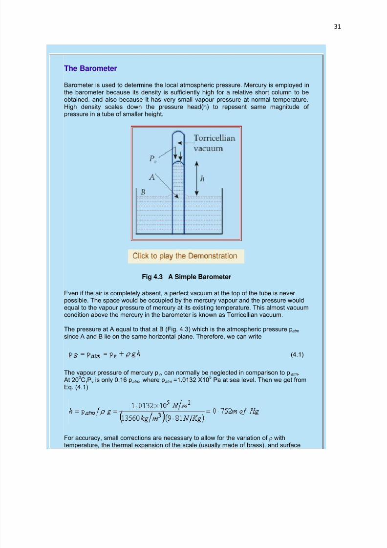
The Barometer
Barometer is used to determine the local atmospheric pressure. Mercury is employed inthe barometer because its density is sufficiently high for a relative short column to beobtained. and also because it has very small vapour pressure at normal temperature.High density scales down the pressure head(h) to repesent same magnitude of pressure in a tube of smaller height.
Fig 4.3 A Simple Barometer
Even if the air is completely absent, a perfect vacuum at the top of the tube is never possible. The space would be occupied by the mercury vapour and the pressure wouldequal to the vapour pressure of mercury at its existing temperature. This almost vacuumcondition above the mercury in the barometer is known as Torricellian vacuum.
The pressure at A equal to that at B (Fig. 4.3) which is the atmospheric pressure patm since A and B lie on the same horizontal plane. Therefore, we can write
(4.1)
The vapour pressure of mercury pv, can normally be neglected in comparison to p atm . At 20
0C,Pv is only 0.16 patm , where patm =1.0132 X10
5Pa at sea level. Then we get from
Eq. (4.1)
For accuracy, small corrections are necessary to allow for the variation of withtemperature, the thermal expansion of the scale (usually made of brass). and surface
7/29/2019 FLUID MECHANICS LECTURE NOTES
http://slidepdf.com/reader/full/fluid-mechanics-lecture-notes 32/297
32
tension effects. If water was used instead of mercury, the corresponding height of thecolumn would be about 10.4 m provided that a perfect vacuum could be achieved abovethe water. However, the vapour pressure of water at ordinary temperature isappreciable and so the actual height at, say, 15°C would be about 180 mm less thanthis value. Moreover. with a tube smaller in diameter than about 15 mm, surface tensioneffects become significant.
Chapter2 : Fluid Statics
Lecture 4 :
Manometers for measuring Gauge and Vacuum Pressure
Manometers are devices in which columns of a suitable liquid are used to measure the difference inpressure between two points or between a certain point and the atmosphere.
Manometer is needed for measuring large gauge pressures. It is basically the modified form of thepiezometric tube. A common type manometer is like a transparent "U-tube" as shown in Fig. 4.4.

7/29/2019 FLUID MECHANICS LECTURE NOTES
http://slidepdf.com/reader/full/fluid-mechanics-lecture-notes 33/297
33
Fig 4.4 A simple manometer to measuregauge pressure
Fig 4.5 A simple manometer to measurevacuum pressure
One of the ends is connected to a pipe or a container having a fluid (A) whose pressure is to bemeasured while the other end is open to atmosphere. The lower part of the U-tube contains a liquidimmiscible with the fluid A and is of greater density than that of A. This fluid is called the manometricfluid.
The pressures at two points P and Q (Fig. 4.4) in a horizontal plane within the continuous expanse of same fluid (the liquid B in this case) must be equal. Then equating the pressures at P and Q in terms of the heights of the fluids above those points, with the aid of the fundamental equation of hydrostatics (Eq3.16), we have
Hence,
where p1 is the absolute pressure of the fluid A in the pipe or container at its centre line, and p atm is thelocal atmospheric pressure. When the pressure of the fluid in the container is lower than the atmosphericpressure, the liquid levels in the manometer would be adjusted as shown in Fig. 4.5. Hence it becomes,
(4.2)
Chapter2 : Fluid Statics
Lecture 4 :
7/29/2019 FLUID MECHANICS LECTURE NOTES
http://slidepdf.com/reader/full/fluid-mechanics-lecture-notes 34/297
34
Manometers to measure Pressure Difference
A manometer is also frequently used to measure the pressure difference, in course of flow, across a restriction in a horizontal pipe.
Fig 4.6 Manometer measuring pressure difference
The axis of each connecting tube at A and B should be perpendicular to the direction of flow and also for the edges of the connections to be smooth. Applying the principle of hydrostatics at P and Q we have,
(4.3)
where, ρ m is the density of manometric fluid and ρw is the density of the working fluidflowing through the pipe.
We can express the difference of pressure in terms of the difference of heads (height of the working fluid at equilibrium).
(4.4)
Chapter2 : Fluid Statics
Lecture 4 :
7/29/2019 FLUID MECHANICS LECTURE NOTES
http://slidepdf.com/reader/full/fluid-mechanics-lecture-notes 35/297

7/29/2019 FLUID MECHANICS LECTURE NOTES
http://slidepdf.com/reader/full/fluid-mechanics-lecture-notes 36/297
36
Inverted Tube Manometer
For the measurement of small pressure differences in liquids, an inverted U-tubemanometer is used.
Fig 4.8 An Inverted Tube Manometer
Here and the line PQ is taken at the level of the higher meniscus to equatethe pressures at P and Q from the principle of hydrostatics. It may be written that
where represents the piezometric pressure, (z being the vertical height of the point concerned from any reference datum). In case of a horizontal pipe (z1= z2) thedifference in piezometric pressure becomes equal to the difference in the static
pressure. If is sufficiently small, a large value of x may be obtained for a
small value of . Air is used as the manometric fluid. Therefore, is negligible
compared with and hence,
(4.5)
Air may be pumped through a valve V at the top of the manometer until the liquidmenisci are at a suitable level.
7/29/2019 FLUID MECHANICS LECTURE NOTES
http://slidepdf.com/reader/full/fluid-mechanics-lecture-notes 37/297
37
Chapter2 : Fluid Statics
Lecture 4 :
Micromanometer
When an additional gauge liquid is used in a U-tube manometer, a large difference in meniscus levelsmay be obtained for a very small pressure difference.
Fig 4.9 A Micromanometer
The equation of hydrostatic equilibrium at PQ can be written as
where and are the densities of working fluid, gauge liquid and manometric liquidrespectively.From continuity of gauge liquid,
(4.6)

7/29/2019 FLUID MECHANICS LECTURE NOTES
http://slidepdf.com/reader/full/fluid-mechanics-lecture-notes 38/297
38
(4.7)
If a is very small compared to A
(4.8)
With a suitable choice for the manometric and gauge liquids so that their densities are close
a reasonable value of y may be achieved for a small pressure difference.
End of Lecture 4!
To start next lecture click next buttonor select from left-hand-side.
Chapter 2 : Fluid Statics
Lecture 5 :
Hydrostatic Thrusts on Submerged Plane Surface
Due to the existence of hydrostatic pressure in a fluid mass, a normal force is exertedon any part of a solid surface which is in contact with a fluid. The individual forcesdistributed over an area give rise to a resultant force.
Plane Surfaces
Consider a plane surface of arbitrary shape wholly submerged in a liquid so that theplane of the surface makes an angle θ with the free surface of the liquid. We willassume the case where the surface shown in the figure below is subjected tohydrostatic pressure on one side and atmospheric pressure on the other side.

7/29/2019 FLUID MECHANICS LECTURE NOTES
http://slidepdf.com/reader/full/fluid-mechanics-lecture-notes 39/297
39
Fig 5.1 Hydrostatic Thrust on Submerged Inclined Plane Surface
Let p denotes the gauge pressure on an elemental area dA. The resultant force F on thearea A is therefore
(5.1)
According to Eq (3.16a) Eq (5.1) reduces to
(5.2)
Where h is the vertical depth of the elemental area dA from the free surface andthe distance y is measured from the x-axis, the line of intersection between theextension of the inclined plane and the free surface (Fig. 5.1). The ordinate of the centreof area of the plane surface A is defined as
(5.3)
7/29/2019 FLUID MECHANICS LECTURE NOTES
http://slidepdf.com/reader/full/fluid-mechanics-lecture-notes 40/297
40
Hence from Eqs (5.2) and (5.3), we get
(5.4)
where is the vertical depth (from free surface) of centre c of area .
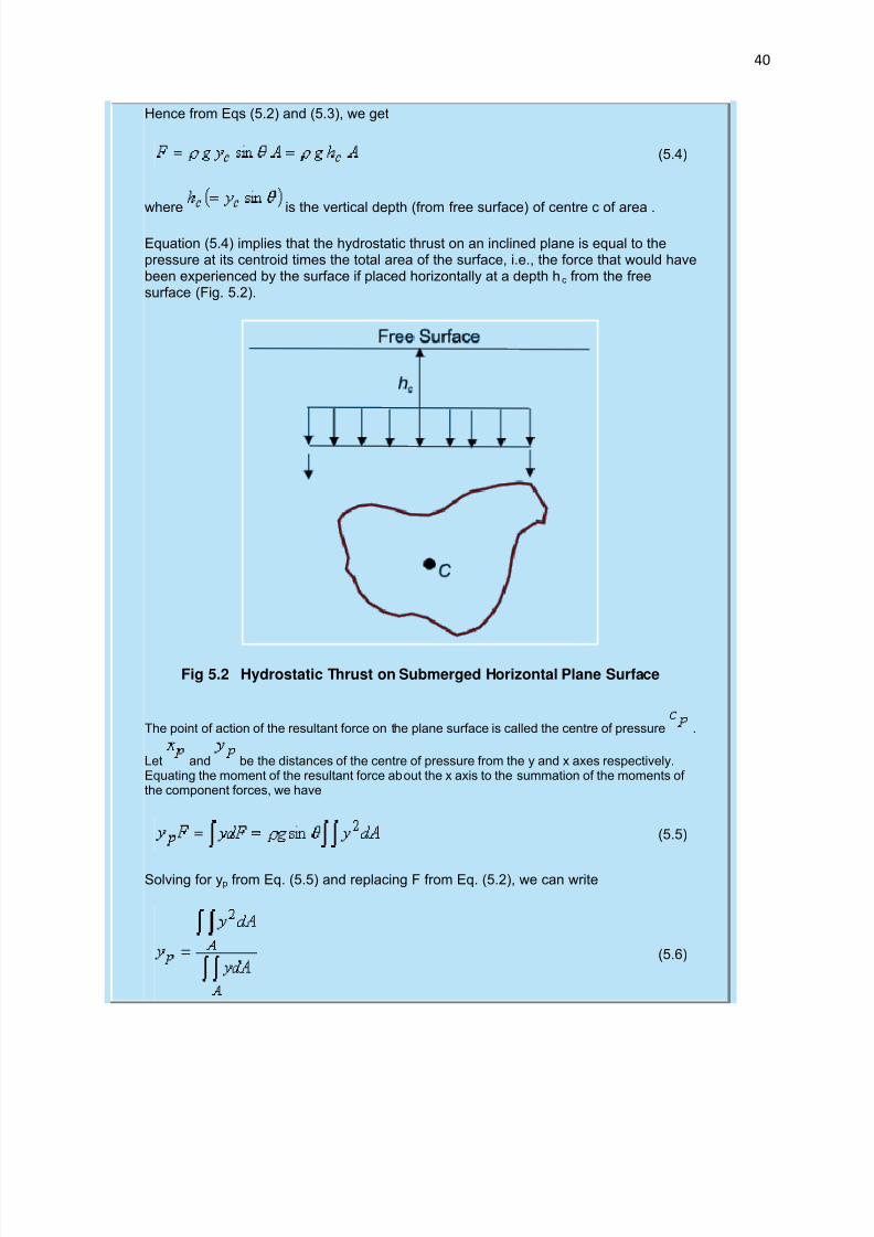
Equation (5.4) implies that the hydrostatic thrust on an inclined plane is equal to thepressure at its centroid times the total area of the surface, i.e., the force that would havebeen experienced by the surface if placed horizontally at a depth h c from the freesurface (Fig. 5.2).
Fig 5.2 Hydrostatic Thrust on Submerged Horizontal Plane Surface
The point of action of the resultant force on the plane surface is called the centre of pressure .
Let and be the distances of the centre of pressure from the y and x axes respectively.Equating the moment of the resultant force about the x axis to the summation of the moments of the component forces, we have
(5.5)
Solving for yp from Eq. (5.5) and replacing F from Eq. (5.2), we can write
(5.6)
7/29/2019 FLUID MECHANICS LECTURE NOTES
http://slidepdf.com/reader/full/fluid-mechanics-lecture-notes 41/297
41
In the same manner, the x coordinate of the centre of pressure can be obtained bytaking moment about the y-axis. Therefore,
From which,
(5.7)
The two double integrals in the numerators of Eqs (5.6) and (5.7) are the moment of
inertia about the x-axis Ixxand the product of inertia Ixy about x and y axis of the plane
area respectively. By applying the theorem of parallel axis
(5.8)
(5.9)
where, and are the moment of inertia and the product of inertia of the surface
about the centroidal axes , and are the coordinates of the center c of the area with respect to x-y axes.
With the help of Eqs (5.8), (5.9) and (5.3), Eqs (5.6) and (5.7) can be written as
(5.10a)
(5.10b)
The first term on the right hand side of the Eq. (5.10a) is always positive. Hence, thecentre of pressure is always at a higher depth from the free surface than that at whichthe centre of area lies. This is obvious because of the typical variation of hydrostatic
pressure with the depth from the free surface. When the plane area is symmetrical
about the y' axis, , and .

7/29/2019 FLUID MECHANICS LECTURE NOTES
http://slidepdf.com/reader/full/fluid-mechanics-lecture-notes 42/297
42
Chapter2 : Fluid Statics
Lecture 3 :
Hydrostatic Thrusts on Submerged Curved Surfaces
On a curved surface, the direction of the normal changes from point to point, and hence thepressure forces on individual elemental surfaces differ in their directions. Therefore, a scalar summation of them cannot be made. Instead, the resultant thrusts in certain directions are to bedetermined and these forces may then be combined vectorially. An arbitrary submerged curvedsurface is shown in Fig. 5.3. A rectangular Cartesian coordinate system is introduced whose xyplane coincides with the free surface of the liquid and z-axis is directed downward below the x -y plane.
Fig 5.3 Hydrostatic thrust on a Submerged Curved Surface
Consider an elemental area dA at a depth z from the surface of the liquid. The hydrostatic forceon the elemental area dA is
(5.11)
and the force acts in a direction normal to the area dA. The components of the force dF in x, yand z directions are
(5.12a)
7/29/2019 FLUID MECHANICS LECTURE NOTES
http://slidepdf.com/reader/full/fluid-mechanics-lecture-notes 43/297
43
(5.12b)
(5.13c)
Where l, m and n are the direction cosines of the normal to dA. The components of the surface
element dA projected on yz, xz and xy planes are, respectively
(5.13a)
(5.13b)
(5.13c)
Substituting Eqs (5.13a-5.13c) into (5.12) we can write
(5.14a)
(5.14b)
(5.14c)
Therefore, the components of the total hydrostatic force along the coordinate axes are
(5.15a)
(5.15b)
(5.15c)
where z c is the z coordinate of the centroid of area Ax and Ay (the projected areas of curvedsurface on yz and xz plane respectively). If z p and y p are taken to be the coordinates of the pointof action of F x on the projected area Ax on yz plane, , we can write
(5.16a)
(5.16b)
where I yy is the moment of inertia of area Ax about y-axis and I yz is the product of inertia of Ax
7/29/2019 FLUID MECHANICS LECTURE NOTES
http://slidepdf.com/reader/full/fluid-mechanics-lecture-notes 44/297
44
with respect to axes y and z. In the similar fashion, z p and x p the coordinates of the point of action of the force F y on area Ay, can be written as
(5.17a)
(5.17b)
where I xx is the moment of inertia of area Ay about x axis and I xz is the product of inertia of Ay about the axes x and z.
We can conclude from Eqs (5.15), (5.16) and (5.17) that for a curved surface, the component of hydrostatic force in a horizontal direction is equal to the hydrostatic force on the projected planesurface perpendicular to that direction and acts through the centre of pressure of the projectedarea. From Eq. (5.15c), the vertical component of the hydrostatic force on the curved surface
can be written as
(5.18)
where is the volume of the body of liquid within the region extending vertically above thesubmerged surface to the free surfgace of the liquid. Therefore, the vertical component of hydrostatic force on a submerged curved surface is equal to the weight of the liquid volumevertically above the solid surface of the liquid and acts through the center of gravity of the liquidin that volume.
Chapter 2 : Fluid Statics
Lecture 5 :

7/29/2019 FLUID MECHANICS LECTURE NOTES
http://slidepdf.com/reader/full/fluid-mechanics-lecture-notes 45/297
45
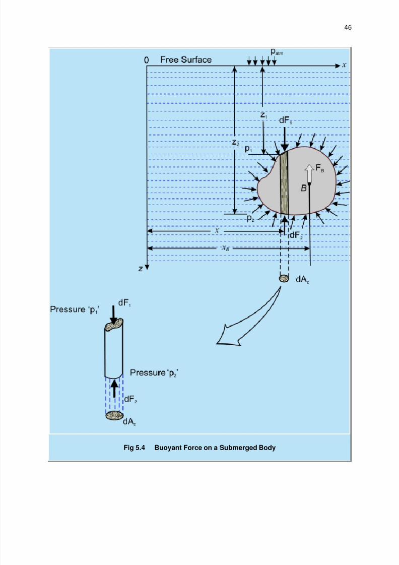
Buoyancy
When a body is either wholly or partially immersed in a fluid, a lift is generated due to the netvertical component of hydrostatic pressure forces experienced by the body.
This lift is called the buoyant force and the phenomenon is called buoyancy Consider a solid body of arbitrary shape completely submerged in a homogeneous liquid as
shown in Fig. 5.4. Hydrostatic pressure forces act on the entire surface of the body.
7/29/2019 FLUID MECHANICS LECTURE NOTES
http://slidepdf.com/reader/full/fluid-mechanics-lecture-notes 46/297
46
Fig 5.4 Buoyant Force on a Submerged Body

7/29/2019 FLUID MECHANICS LECTURE NOTES
http://slidepdf.com/reader/full/fluid-mechanics-lecture-notes 47/297
47
To calculate the vertical component of the resultant hydrostatic force, the body is considered to bedivided into a number of elementary vertical prisms. The vertical forces acting on the two ends of such aprism of cross-section dAz (Fig. 5.4) are respectively
(5.19a)
(5.19b)
Therefore, the buoyant force (the net vertically upward force) acting on the elemental prism of volume
is -
(5.19c)
Hence the buoyant force FB on the entire submerged body is obtained as
(5.20)
Where is the total volume of the submerged body. The line of action of the force F B can be found bytaking moment of the force with respect to z-axis. Thus
(5.21)
Substituting for dFB and FB from Eqs (5.19c) and (5.20) respectively into Eq. (5.21), the x coordinate ofthe center of the buoyancy is obtained as
(5.22)
which is the centroid of the displaced volume. It is found from Eq. (5.20) that the buoyant force FB equals to the weight of liquid displaced by the submerged body of volume . This phenomenon wasdiscovered by Archimedes and is known as the Archimedes principle.
ARCHIMEDES PRINCIPLE
The buoyant force on a submerged body
The Archimedes principle states that the buoyant force on a submerged body is equal to theweight of liquid displaced by the body, and acts vertically upward through the centroid of thedisplaced volume.
Thus the net weight of the submerged body, (the net vertical downward force experienced by it)is reduced from its actual weight by an amount that equals the buoyant force.
7/29/2019 FLUID MECHANICS LECTURE NOTES
http://slidepdf.com/reader/full/fluid-mechanics-lecture-notes 48/297
48
The buoyant force on a partially immersed body
According to Archimedes principle, the buoyant force of a partially immersed body is equal to theweight of the displaced liquid.
Therefore the buoyant force depends upon the density of the fluid and the submerged volume of the body.
For a floating body in static equilibrium and in the absence of any other external force, thebuoyant force must balance the weight of the body.
Let us do an example
Chapter 2 : Fluid Statics
Lecture 5 :
Stability of Unconstrained Submerged Bodies in Fluid
The equilibrium of a body submerged in a liquid requires that the weight of thebody acting through its cetre of gravity should be colinear with an equalhydrostatic lift acting through the centre of buoyancy.
In general, if the body is not homogeneous in its distribution of mass over theentire volume, the location of centre of gravity G does not coincide with thecentre of volume, i.e., the centre of buoyancy B.
Depending upon the relative locations of G and B, a floating or submerged bodyattains three different states of equilibrium-
Let us suppose that a body is given a small angular displacement and then released.Then it will be said to be in
Stable Equilibrium: If the body returns to its original position by retainingthe originally vertical axis as vertical.
Unstable Equilibrium: If the body does not return to its original positionbut moves further from it.
Neutral Equilibrium: If the body neither returns to its original position norincreases its displacement further, it will simply adopt its new position.
7/29/2019 FLUID MECHANICS LECTURE NOTES
http://slidepdf.com/reader/full/fluid-mechanics-lecture-notes 49/297
49
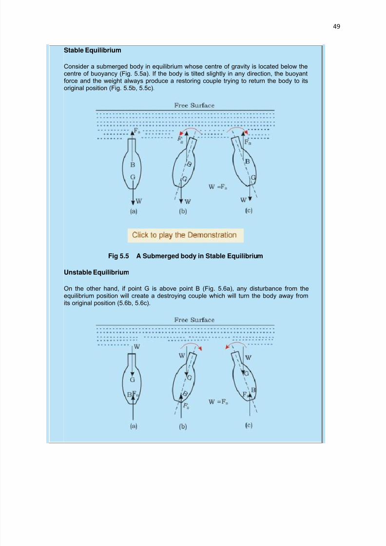
Stable Equilibrium
Consider a submerged body in equilibrium whose centre of gravity is located below thecentre of buoyancy (Fig. 5.5a). If the body is tilted slightly in any direction, the buoyantforce and the weight always produce a restoring couple trying to return the body to itsoriginal position (Fig. 5.5b, 5.5c).
Fig 5.5 A Submerged body in Stable Equilibrium
Unstable Equilibrium
On the other hand, if point G is above point B (Fig. 5.6a), any disturbance from theequilibrium position will create a destroying couple which will turn the body away fromits original position (5.6b, 5.6c).

7/29/2019 FLUID MECHANICS LECTURE NOTES
http://slidepdf.com/reader/full/fluid-mechanics-lecture-notes 50/297
50
Fig 5.6 A Submerged body in Unstable Equilibrium
Neutral Equilibrium
When the centre of gravity G and centre of buoyancy B coincides, the body will alwaysassume the same position in which it is placed (Fig 5.7) and hence it is in neutralequilibrium.
Fig 5.7 A Submerged body in Neutral Equilibrium
Therefore, it can be concluded that a submerged body will be in stable, unstable orneutral equilibrium if its centre of gravity is below, above or coincident with thecenter of buoyancy respectively (Fig. 5.8).

7/29/2019 FLUID MECHANICS LECTURE NOTES
http://slidepdf.com/reader/full/fluid-mechanics-lecture-notes 51/297
51
Fig 5.8 States of Equilibrium of a Submerged Body
(a) STABLE EQUILIBRIUM (B) UNSTABLE EQUILIBRIUM (C) NEUTRALEQUILIBRIUM
Chapter2 : Fluid Statics
Lecture 5 :
7/29/2019 FLUID MECHANICS LECTURE NOTES
http://slidepdf.com/reader/full/fluid-mechanics-lecture-notes 52/297
52
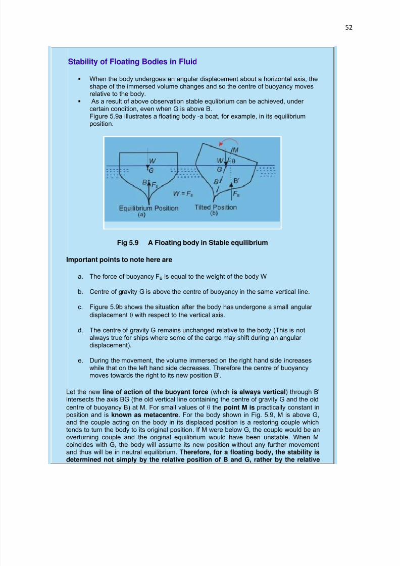
Stability of Floating Bodies in Fluid
When the body undergoes an angular displacement about a horizontal axis, theshape of the immersed volume changes and so the centre of buoyancy movesrelative to the body.
As a result of above observation stable equlibrium can be achieved, under certain condition, even when G is above B.Figure 5.9a illustrates a floating body -a boat, for example, in its equilibriumposition.
Fig 5.9 A Floating body in Stable equilibrium
Important points to note here are
a. The force of buoyancy FB is equal to the weight of the body W
b. Centre of gravity G is above the centre of buoyancy in the same vertical line.
c. Figure 5.9b shows the situation after the body has undergone a small angular
displacement with respect to the vertical axis.
d. The centre of gravity G remains unchanged relative to the body (This is notalways true for ships where some of the cargo may shift during an angular displacement).
e. During the movement, the volume immersed on the right hand side increaseswhile that on the left hand side decreases. Therefore the centre of buoyancymoves towards the right to its new position B'.
Let the new line of action of the buoyant force (which is always vertical) through B'intersects the axis BG (the old vertical line containing the centre of gravity G and the old
centre of buoyancy B) at M. For small values of the point M is practically constant inposition and is known as metacentre. For the body shown in Fig. 5.9, M is above G,and the couple acting on the body in its displaced position is a restoring couple whichtends to turn the body to its original position. If M were below G, the couple would be anoverturning couple and the original equilibrium would have been unstable. When Mcoincides with G, the body will assume its new position without any further movementand thus will be in neutral equilibrium. Therefore, for a floating body, the stability isdetermined not simply by the relative position of B and G, rather by the relative

7/29/2019 FLUID MECHANICS LECTURE NOTES
http://slidepdf.com/reader/full/fluid-mechanics-lecture-notes 53/297
53
position of M and G. The distance of metacentre above G along the line BG is knownas metacentric height GM which can be written as
GM = BM -BG
Hence the condition of stable equilibrium for a floating body can be expressed in
terms of metacentric height as follows:
GM > 0 (M is above G) Stable equilibrium
GM = 0 (M coinciding with G) Neutral equilibrium
GM < 0 (M is below G) Unstable equilibrium
The angular displacement of a boat or ship about its longitudinal axis is known as'rolling' while that about its transverse axis is known as "pitching".
Floating Bodies Containing Liquid
If a floating body carrying liquid with a free surface undergoes an angular displacement,
the liquid will also move to keep its free surface horizontal. Thus not only does thecentre of buoyancy B move, but also the centre of gravity G of the floating body and itscontents move in the same direction as the movement of B. Hence the stability of thebody is reduced. For this reason, liquid which has to be carried in a ship is put into anumber of separate compartments so as to minimize its movement within the ship.
Chapter 2 : Fluid Statics
Lecture 5 :
7/29/2019 FLUID MECHANICS LECTURE NOTES
http://slidepdf.com/reader/full/fluid-mechanics-lecture-notes 54/297
54
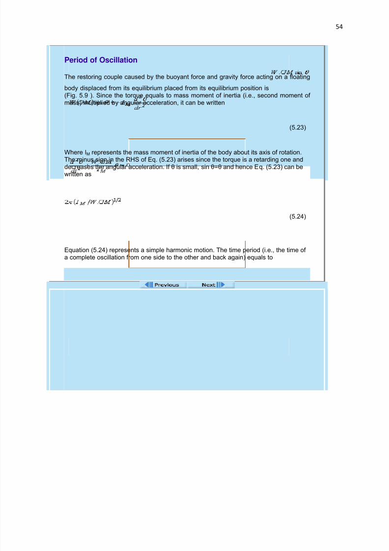
Period of Oscillation
The restoring couple caused by the buoyant force and gravity force acting on a floating
body displaced from its equilibrium placed from its equilibrium position is
(Fig. 5.9 ). Since the torque equals to mass moment of inertia (i.e., second moment of mass) multiplied by angular acceleration, it can be written
(5.23)
Where IM represents the mass moment of inertia of the body about its axis of rotation.The minus sign in the RHS of Eq. (5.23) arises since the torque is a retarding one anddecreases the angular acceleration. If θ is small, sin θ=θ and hence Eq. (5.23) can bewritten as
(5.24)
Equation (5.24) represents a simple harmonic motion. The time period (i.e., the time of a complete oscillation from one side to the other and back again) equals to
. The oscillation of the body results in a flow of the liquid around itand this flow has been disregarded here. In practice, of course, viscosity in the liquid
introduces a damping action which quickly suppresses the oscillation unless further disturbances such as waves cause new angular displacements.
End of Lecture 5!
To view the exercise problem, clicknext button or select from left-hand-side.

7/29/2019 FLUID MECHANICS LECTURE NOTES
http://slidepdf.com/reader/full/fluid-mechanics-lecture-notes 55/297
55
Module 2 :
Chapter 3 : Kinematics of Fluid
The chapter contains
Lecture 6
Kinematics
Scalar and Vector Fields
Flow Field and Description of Fluid Motion
Lecture 7
Variation of Flow Parameter in Time and Space
Material Derivative and Acceleration
Streamlines, Path Lines and Streak Lines
Lecture 8
One, Two and Three Dimensional Flows
Translation, Rate of Deformation and Rotation
Vorticity
Existence of Flows
Exercise Problem
7/29/2019 FLUID MECHANICS LECTURE NOTES
http://slidepdf.com/reader/full/fluid-mechanics-lecture-notes 56/297
56
Chapter 3 : Kinematics of Fluid
Lecture 6 :
KINEMATICS OF FLUID
Introduction
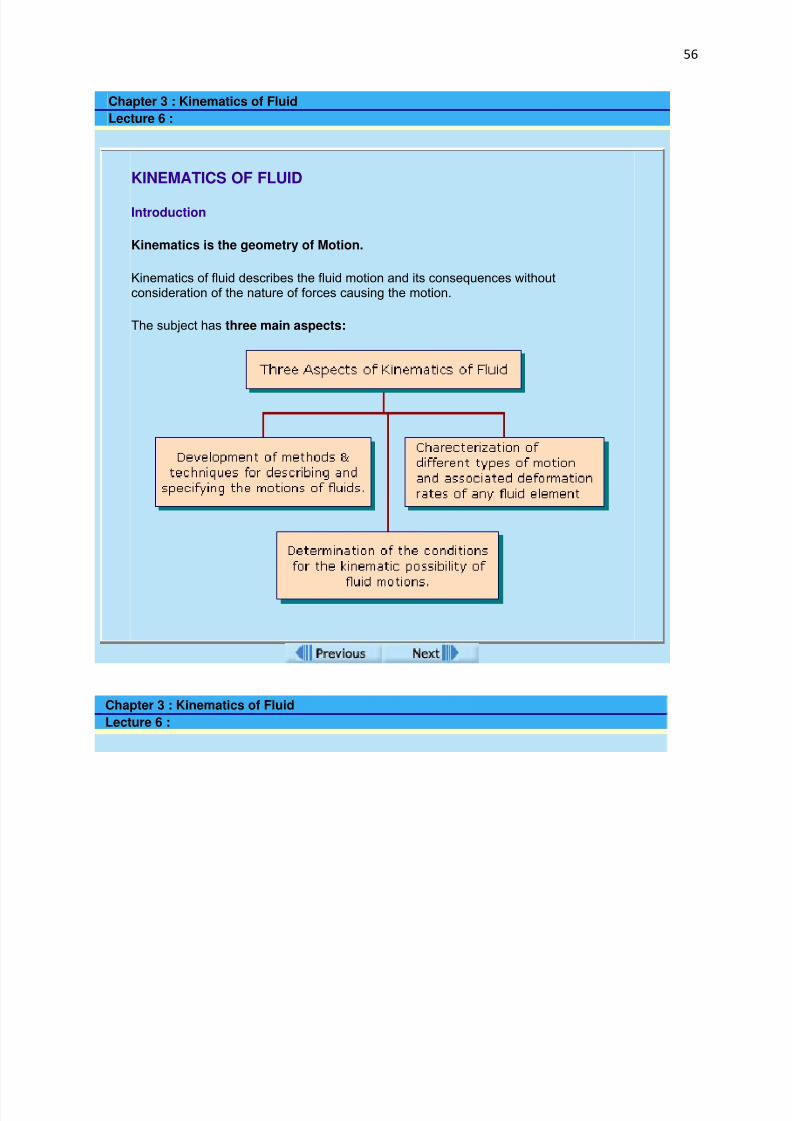
Kinematics is the geometry of Motion.
Kinematics of fluid describes the fluid motion and its consequences withoutconsideration of the nature of forces causing the motion.
The subject has three main aspects:
Chapter 3 : Kinematics of Fluid
Lecture 6 :
7/29/2019 FLUID MECHANICS LECTURE NOTES
http://slidepdf.com/reader/full/fluid-mechanics-lecture-notes 57/297
57
Scalar and Vector Fields
Scalar: Scalar is a quantity which can be expressed by a single number representingits magnitude.
Example: mass, density and temperature.
Scalar Field
If at every point in a region, a scalar function has a defined value, the region is calleda scalar field.Example: Temperature distribution in a rod.
Vector: Vector is a quantity which is specified by both magnitude and direction.Example: Force, Velocity and Displacement.
Vector Field
If at every point in a region, a vector function has a defined value, the region is calleda vector field.Example: velocity field of a flowing fluid .
Flow Field
The region in which the flow parameters i.e. velocity, pressure etc. are defined at eachand every point at any instant of time is called a flow field.
Thus a flow field would be specified by the velocities at different points in the region atdifferent times.
Chapter 3 : Kinematics of Fluid
Lecture 6 :
7/29/2019 FLUID MECHANICS LECTURE NOTES
http://slidepdf.com/reader/full/fluid-mechanics-lecture-notes 58/297
58
Description of Fluid Motion
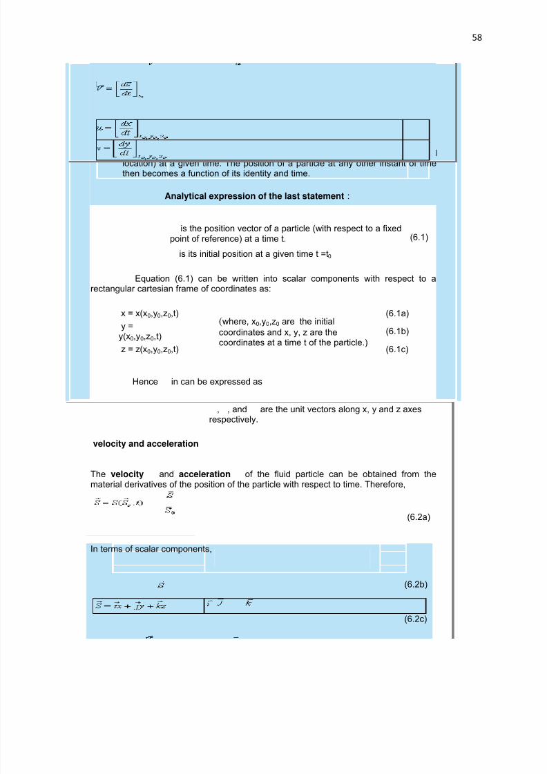
A. Lagrangian Method
Using Lagrangian method, the fluid motion is described by tracing thekinematic behaviour of each particle constituting the flow. Identities of the particles are made by specifying their initial position (spatial
location) at a given time. The position of a particle at any other instant of timethen becomes a function of its identity and time.
Analytical expression of the last statement :
is the position vector of a particle (with respect to a fixedpoint of reference) at a time t.
is its initial position at a given time t =t0
(6.1)
Equation (6.1) can be written into scalar components with respect to arectangular cartesian frame of coordinates as:
x = x(x0,y0,z0,t)(where, x0,y0,z0 are the initial
coordinates and x, y, z are thecoordinates at a time t of the particle.)
(6.1a)
y =y(x0,y0,z0,t)
(6.1b)
z = z(x0,y0,z0,t) (6.1c)
Hence in can be expressed as
, , and are the unit vectors along x, y and z axesrespectively.
velocity and acceleration
The velocity and acceleration of the fluid particle can be obtained from thematerial derivatives of the position of the particle with respect to time. Therefore,
(6.2a)
In terms of scalar components,
(6.2b)
(6.2c)

7/29/2019 FLUID MECHANICS LECTURE NOTES
http://slidepdf.com/reader/full/fluid-mechanics-lecture-notes 59/297
59
(6.2d)
where u, v, w are the components of velocity in x, y, z directions respectively.
Similarly, for the acceleration,
(6.3a)
and hence,
(6.3b)
(6.3c)
(6.3d)
where ax, ay, az are accelerations in x, y, z directions respectively.
Advantages of Lagrangian Method:
1. Since motion and trajectory of each fluid particle is known, its history can betraced.
2. Since particles are identified at the start and traced throughout their motion,conservation of mass is inherent.
Disadvantages of Lagrangian Method:
1. The solution of the equations presents appreciable mathematical difficultiesexcept certain special cases and therefore, the method is rarely suitable for practical applications.
Chapter 3 : Kinematics of Fluid
Lecture 6 :
7/29/2019 FLUID MECHANICS LECTURE NOTES
http://slidepdf.com/reader/full/fluid-mechanics-lecture-notes 60/297
60
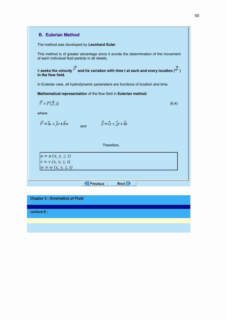
B. Eulerian Method
The method was developed by Leonhard Euler.
This method is of greater advantage since it avoids the determination of the movementof each individual fluid particle in all details.
It seeks the velocity and its variation with time t at each and every location ( )in the flow field.
In Eulerian view, all hydrodynamic parameters are functions of location and time.
Mathematical representation of the flow field in Eulerian method:
(6.4)
where
and
Therefore,
u = u (x, y, z, t)
v = v (x, y, z, t)
w = w (x, y, z, t)
Chapter 3 : Kinematics of Fluid
Lecture 6 :
7/29/2019 FLUID MECHANICS LECTURE NOTES
http://slidepdf.com/reader/full/fluid-mechanics-lecture-notes 61/297
61
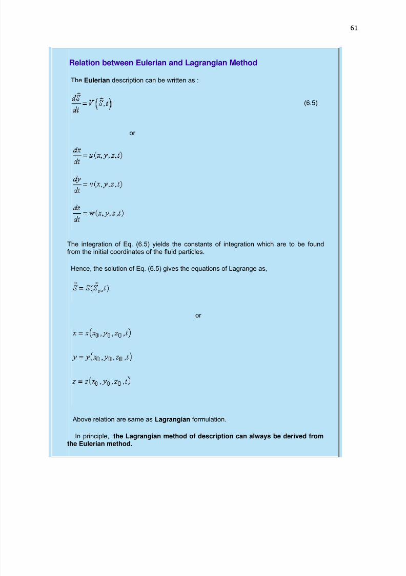
Relation between Eulerian and Lagrangian Method
The Eulerian description can be written as :
(6.5)
or
The integration of Eq. (6.5) yields the constants of integration which are to be foundfrom the initial coordinates of the fluid particles.
Hence, the solution of Eq. (6.5) gives the equations of Lagrange as,
or
Above relation are same as Lagrangian formulation.
In principle, the Lagrangian method of description can always be derived fromthe Eulerian method.
7/29/2019 FLUID MECHANICS LECTURE NOTES
http://slidepdf.com/reader/full/fluid-mechanics-lecture-notes 62/297
62
Let us do an example
End of Lecture 6!
To start next lecture click next
button or select from left-hand-
side.
Chapter 3 : Kinematics of Fluid
Lecture 7 :
Variation of Flow Parameters in Time and Space
Hydrodynamic parameters like pressure and density along with flow velocity may varyfrom one point to another and also from one instant to another at a fixed point.
According to type of variations, categorizing the flow:
Steady and Unsteady Flow
Steady Flow A steady flow is defined as a flow in which the various hydrodynamicparameters and fluid properties at any point do not change with time.
In Eulerian approach, a steady flow is described as,
and

7/29/2019 FLUID MECHANICS LECTURE NOTES
http://slidepdf.com/reader/full/fluid-mechanics-lecture-notes 63/297
7/29/2019 FLUID MECHANICS LECTURE NOTES
http://slidepdf.com/reader/full/fluid-mechanics-lecture-notes 64/297
64
Uniform and Non-uniform Flows
Uniform Flow
The flow is defined as uniform flow when in the flow field the velocity and otherhydrodynamic parameters do not change f rom point to point at any instant oftime.
For a uniform flow, the velocity is a function of time only, which can be expressed inEulerian description as
Implication:
1. For a uniform flow, there will be no spatial distribution of hydrodynamic and
other parameters.
2. Any hydrodynamic parameter will have a unique value in the entire field,irrespective of whether it
changes with time − unsteady uniform flow OR
does not change with time − steady uniform flow.
3. Thus ,steadiness of flow and uniformity of flow does not necessarily gotogether.
Non-Uniform Flow
When the velocity and other hydrodynamic parameters changes from onepoint to another the flow is defined as non-uniform.
Important points:
1. For a non-uniform flow, the changes with position may be found either in thedirection of flow or in directions perpendicular to it.
2.Non-uniformity in a direction perpendicular to the flow is always encounterednear solid boundaries past which the fluid flows.
Reason: All fluids possess viscosity which reduces the relative velocity (of the fluidw.r.t. to the wall) to zero at a solid boundary. This is known as no-slip condition.
Four possible combinations

7/29/2019 FLUID MECHANICS LECTURE NOTES
http://slidepdf.com/reader/full/fluid-mechanics-lecture-notes 65/297
65
Type Example
1. Steady Uniform flow Flow at constant rate through a duct of uniform cross-section (The region close tothe walls of the duct is disregarded)
2. Steady non-uniform flowFlow at constant rate through a duct of non-
uniform cross-section (tapering pipe)
3. Unsteady Uniform flow Flow at varying rates through a long straightpipe of uniform cross-section. (Again theregion close to the walls is ignored.)
4. Unsteady non-uniformflow
Flow at varying rates through a duct of non-uniform cross-section.
Chapter 3 : Kinematics of Fluid
Lecture 7 :
Material Derivative and Acceleration
Let the position of a particle at any instant t in a flow field be given by the spacecoordinates (x, y, z) with respect to a rectangular cartesian frame of reference.
The velocity components u, v, w of the particle along x, y and z directions respectivelycan then be written in Eulerian form as
u = u (x, y, z, t)v = v (x, y, z, t)w = w (x, y, z, t)
After an infinitesimal time interval t , let the particle move to a new position given by the
coordinates ( x + Δ x, y +Δy , z + Δ z). Its velocity components at this new position be u + Δu, v + Δv and w +Δw.
Expression of velocity components in the Taylor's series form:
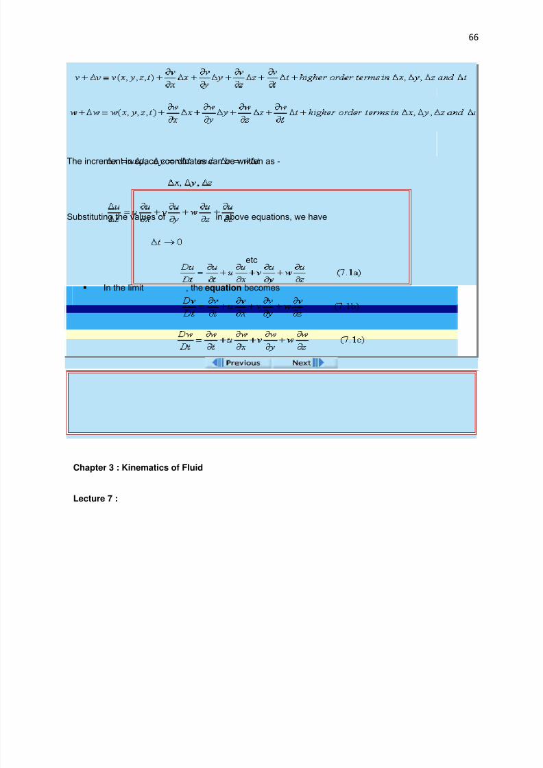
7/29/2019 FLUID MECHANICS LECTURE NOTES
http://slidepdf.com/reader/full/fluid-mechanics-lecture-notes 66/297
66
The increment in space coordinates can be written as -
Substituting the values of in above equations, we have
etc
In the limit , the equation becomes
Chapter 3 : Kinematics of Fluid
Lecture 7 :

7/29/2019 FLUID MECHANICS LECTURE NOTES
http://slidepdf.com/reader/full/fluid-mechanics-lecture-notes 67/297
67
Material Derivation and Acceleration...contd. from previous slide
The above equations tell that the operator for total differential with respect totime, D/Dt in a convective field is related to the partial differential as:
Explanation of equation 7.2 :
The total differential D/Dt is known as the material or substantial derivative with respect to time.
The first term t in the right hand side of is known as temporal or localderivative which expresses the rate of change with time, at a fixed position.
The last three terms in the right hand side of are together known as
convective derivative which represents the time rate of change due to changein position in the field.
Explanation of equation 7.1 (a, b, c):
The terms in the left hand sides of Eqs (7.1a) to (7.1c) are defined as x, y and zcomponents of substantial or material acceleration.
The first terms in the right hand sides of Eqs (7.1a) to (7.1c) represent therespective local or temporal accelerations, while the other termsare convective accelerations.
Thus we can write,
(Material or substantial acceleration) = (temporal or local acceleration) +(convective acceleration)
Important points:
1. In a steady flow, the temporal acceleration is zero, since the velocity at any

7/29/2019 FLUID MECHANICS LECTURE NOTES
http://slidepdf.com/reader/full/fluid-mechanics-lecture-notes 68/297
68
point is invariant with time.
2. In a uniform flow, on the other hand, the convective acceleration is zero, sincethe velocity components are not the functions of space coordinates.
3. In a steady and uniform flow, both the temporal and convective acceleration
vanish and hence there exists no material acceleration.
Existence of the components of acceleration for different types of flow is shown inthe table below.
Type of Flow Material Acceleration
Temporal Convective
1. Steady Uniform flow 0 0
2. Steady non-uniformflow 0 exists
3. Unsteady Uniform flow exists 0
4. Unsteady non-uniform
flowexists exists
Let us do an example
Chapter 3 : Kinematics of Fluid
Lecture 7 :
In vector form, Components of Acceleration in Cylindrical Polar Coordinate System ( r, , z )
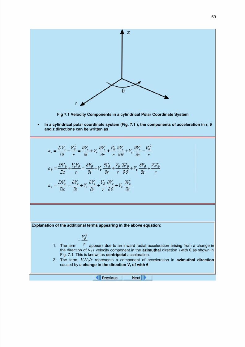
7/29/2019 FLUID MECHANICS LECTURE NOTES
http://slidepdf.com/reader/full/fluid-mechanics-lecture-notes 69/297
7/29/2019 FLUID MECHANICS LECTURE NOTES
http://slidepdf.com/reader/full/fluid-mechanics-lecture-notes 70/297
70
Chapter 3 : Kinematics of Fluid
Lecture 7 :
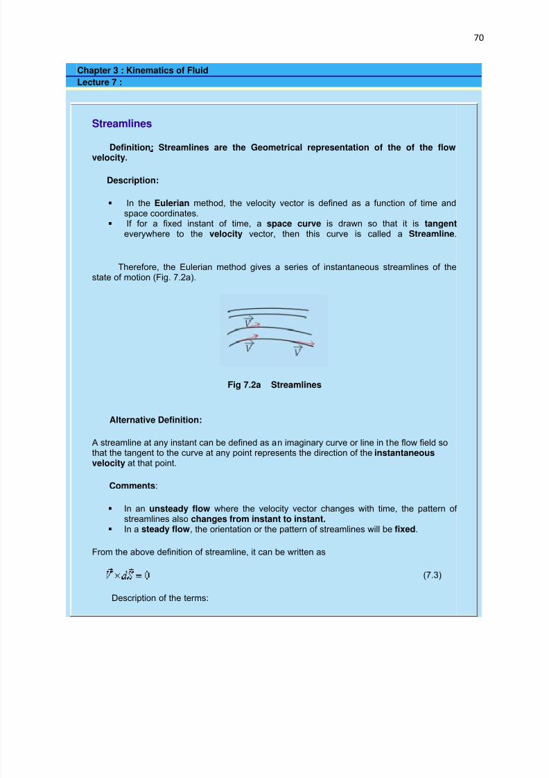
Streamlines
Definition: Streamlines are the Geometrical representation of the of the flowvelocity.
Description:
In the Eulerian method, the velocity vector is defined as a function of time andspace coordinates.
If for a fixed instant of time, a space curve is drawn so that it is tangenteverywhere to the velocity vector, then this curve is called a Streamline.
Therefore, the Eulerian method gives a series of instantaneous streamlines of thestate of motion (Fig. 7.2a).
Fig 7.2a Streamlines
Alternative Definition:
A streamline at any instant can be defined as an imaginary curve or line in the flow field sothat the tangent to the curve at any point represents the direction of the instantaneousvelocity at that point.
Comments:
In an unsteady flow where the velocity vector changes with time, the pattern of streamlines also changes from instant to instant.
In a steady flow, the orientation or the pattern of streamlines will be fixed.
From the above definition of streamline, it can be written as
(7.3)
Description of the terms:

7/29/2019 FLUID MECHANICS LECTURE NOTES
http://slidepdf.com/reader/full/fluid-mechanics-lecture-notes 71/297
71
1. is the length of an infinitesimal line segment along a streamline at a point .
2. is the instantaneous velocity vector.
The above expression therefore represents the differential equation of a streamline. In acartesian coordinate-system, representing
the above equation ( Equation 7.3 ) may be simplified as
(7.4)
Stream tube:
A bundle of neighboring streamlines may be imagined to form a passage through which thefluid flows. This passage is known as a stream-tube.
Fig 7.2b Stream Tube
Properties of Stream tube:
1. The stream-tube is bounded on all sides by streamlines.
2. Fluid velocity does not exist across a streamline, no fluid may enter or leave astream-tube except through its ends.
3. The entire flow in a flow field may be imagined to be composed of flows throughstream-tubes arranged in some arbitrary positions.
Chapter 3 : Kinematics of Fluid
Lecture 7 :
7/29/2019 FLUID MECHANICS LECTURE NOTES
http://slidepdf.com/reader/full/fluid-mechanics-lecture-notes 72/297
72
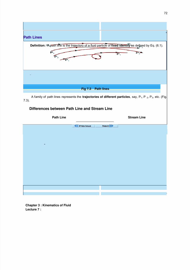
Path Lines
Definition: A path line is the trajectory of a fluid particle of fixed identity as defined by Eq. (6.1).
Fig 7.3 Path lines
A family of path lines represents the trajectories of different particles, say, P1, P 2, P3, etc. (Fig.7.3).
Differences between Path Line and Stream Line
Path Line Stream Line
This refers to a path followed by a fluid particleover a period of time.
This is an imaginary curve in a flow field f
fixed instant of time, tangent to which g
the instantaneous velocity at that point .
Two path lines can intersect each other as or a single
path line can form a loop as different particles or
even same particle can arrive at the same point at
different instants of time.
Two stream lines can never intersect e
other, as the instantaneous velocity vect
any given point is unique.
Note: In a steady flow path lines are identical to streamlines as the Eulerian and Lagrangian versions become the same.
Lets Do Some Examples
Chapter 3 : Kinematics of Fluid
Lecture 7 :

7/29/2019 FLUID MECHANICS LECTURE NOTES
http://slidepdf.com/reader/full/fluid-mechanics-lecture-notes 73/297
73
Streak Lines
Definition: A streak line is the locus of the temporary locations of all particles thathave passed though a fixed point in the flow field at any instant of time.
Features of a Streak Line:
While a path line refers to the identity of a fluid particle, a streak line is specifiedby a fixed point in the flow field.
It is of particular interest in experimental flow visualization. Example: If dye is injected into a liquid at a fixed point in the flow field, then at
a later time t, the dye will indicate the end points of the path lines of particleswhich have passed through the injection point.
The equation of a streak line at time t can be derived by the Lagrangianmethod.
If a fluid particle passes through a fixed point in course of time t, then theLagrangian method of description gives the equation
(7.5)
Solving for ,
(7.6)
If the positions of the particles which have passed through the fixed point aredetermined, then a streak line can be drawn through these points.
Equation: The equation of the streak line at a time t is given by
(7.7)
Substituting Eq. (7.5) into Eq. (7.6) we get the final form of equation of the streakline,
(7.8)
Chapter 3 : Kinematics of Fluid
Lecture 8 :

7/29/2019 FLUID MECHANICS LECTURE NOTES
http://slidepdf.com/reader/full/fluid-mechanics-lecture-notes 74/297
74
One, Two and Three Dimensional Flows
Fluid flow is three-dimensional in nature.
This means that the flow parameters like velocity, pressure and so on vary in allthe three coordinate directions.
Sometimes simplification is made in the analysis of different fluid flow problems by:
Selecting the appropriate coordinate directions so that appreciable variation of the hydro dynamic parameters take place in only two directions or even in onlyone.
One-dimensional flow
All the flow parameters may be expressed as functions of time and one spacecoordinate only.
The single space coordinate is usually the distance measured along the centre-line (not necessarily straight) in which the fluid is flowing.
Example: the flow in a pipe is considered one-dimensional when variations of pressure and velocity occur along the length of the pipe, but any variation over the cross-section is assumed negligible.
In reality, flow is never one-dimensional because viscosity causes the velocityto decrease to zero at the solid boundaries.
If however, the non uniformity of the actual flow is not too great, valuableresults may often be obtained from a "one dimensional analysis".
The average values of the flow parameters at any given section (perpendicular to the flow) are assumed to be applied to the entire flow at that section.
Two-dimensional flow
All the flow parameters are functions of time and two space coordinates (say xand y).
No variation in z direction.
The same streamline patterns are found in all planes perpendicular to zdirection at any instant.
Three dimensional flow
The hydrodynamic parameters are functions of three space coordinates andtime.
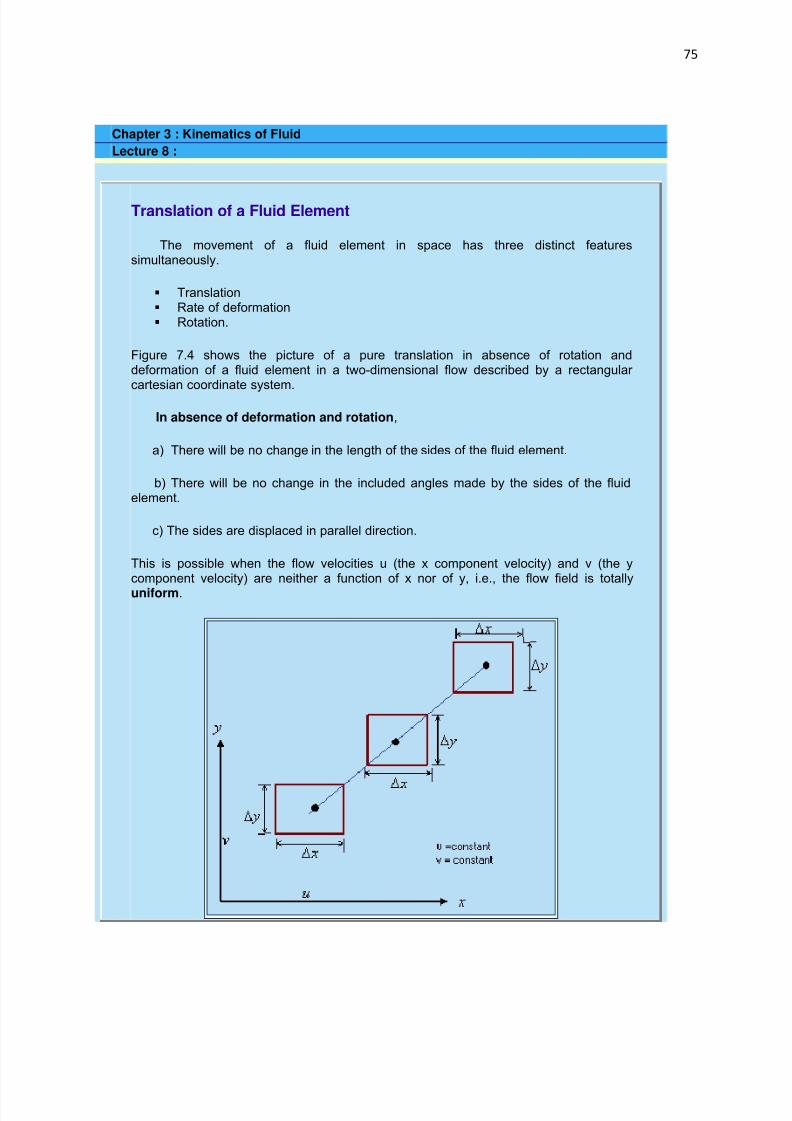
7/29/2019 FLUID MECHANICS LECTURE NOTES
http://slidepdf.com/reader/full/fluid-mechanics-lecture-notes 75/297
75
Chapter 3 : Kinematics of Fluid
Lecture 8 :
Translation of a Fluid Element
The movement of a fluid element in space has three distinct featuressimultaneously.
Translation Rate of deformation Rotation.
Figure 7.4 shows the picture of a pure translation in absence of rotation anddeformation of a fluid element in a two-dimensional flow described by a rectangular cartesian coordinate system.
In absence of deformation and rotation,
a) There will be no change in the length of the sides of the fluid element.
b) There will be no change in the included angles made by the sides of the fluidelement.
c) The sides are displaced in parallel direction.
This is possible when the flow velocities u (the x component velocity) and v (the ycomponent velocity) are neither a function of x nor of y, i.e., the flow field is totally
uniform.
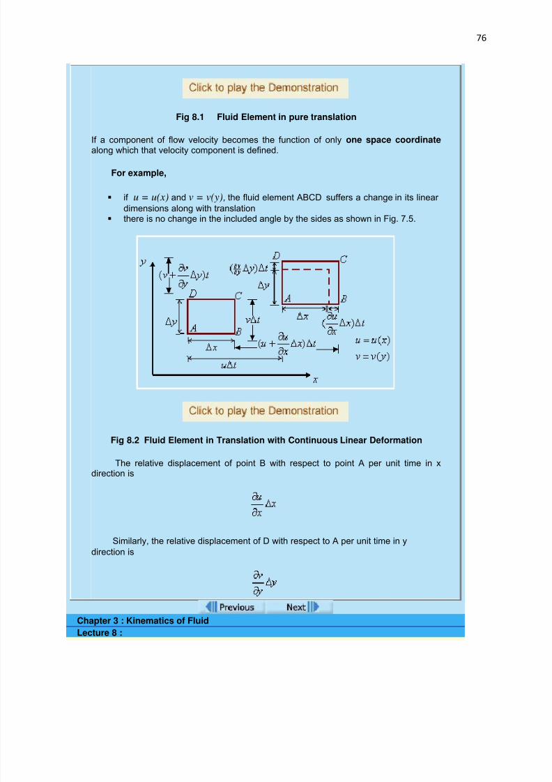
7/29/2019 FLUID MECHANICS LECTURE NOTES
http://slidepdf.com/reader/full/fluid-mechanics-lecture-notes 76/297
76
Fig 8.1 Fluid Element in pure translation
If a component of flow velocity becomes the function of only one space coordinate along which that velocity component is defined.
For example,
if u = u(x) and v = v(y), the fluid element ABCD suffers a change in its linear
dimensions along with translation there is no change in the included angle by the sides as shown in Fig. 7.5.
Fig 8.2 Fluid Element in Translation with Continuous Linear Deformation
The relative displacement of point B with respect to point A per unit time in xdirection is
Similarly, the relative displacement of D with respect to A per unit time in y
direction is
Chapter 3 : Kinematics of Fluid
Lecture 8 :
7/29/2019 FLUID MECHANICS LECTURE NOTES
http://slidepdf.com/reader/full/fluid-mechanics-lecture-notes 77/297
77
Translation with Linear Deformations
Observations from the figure:
Since u is not a function of y and v is not a function of x
All points on the linear element AD move with same velocity in the x direction.
All points on the linear element AB move with the same velocity in y direction.
Hence the sides move parallel from their initial position without changing theincluded angle.
This situation is referred to as translation with linear deformation.
Strain rate:
The changes in lengths along the coordinate axes per unit time per unit original lengthsare defined as the components of linear deformation or strain rate in therespective directions.
Therefore, linear strain rate component in the x direction
and, linear strain rate component in y direction
Rate of Deformation in the Fluid Element
Let us consider both the velocity component u and v are functions of x and y, i.e.,
u = u(x,y)
v = v(x,y)
Figure 8.3 represent the above condition
Observations from the figure:
Point B has a relative displacement in y direction with respect to the point A. Point D has a relative displacement in x direction with respect to point A. The included angle between AB and AD changes.

7/29/2019 FLUID MECHANICS LECTURE NOTES
http://slidepdf.com/reader/full/fluid-mechanics-lecture-notes 78/297
78
The fluid element suffers a continuous angular deformation along with the linear deformations in course of its motion.
Rate of Angular deformation:
The rate of angular deformation is defined as the rate of change of angle between the
linear segments AB and AD which were initially perpendicular to each other.
Fig 8.3 Fluid element in translation with simultaneous linear and angulardeformation rates
From the above figure rate of angular deformation,
(8.1)
From the geometry
(8.2a)
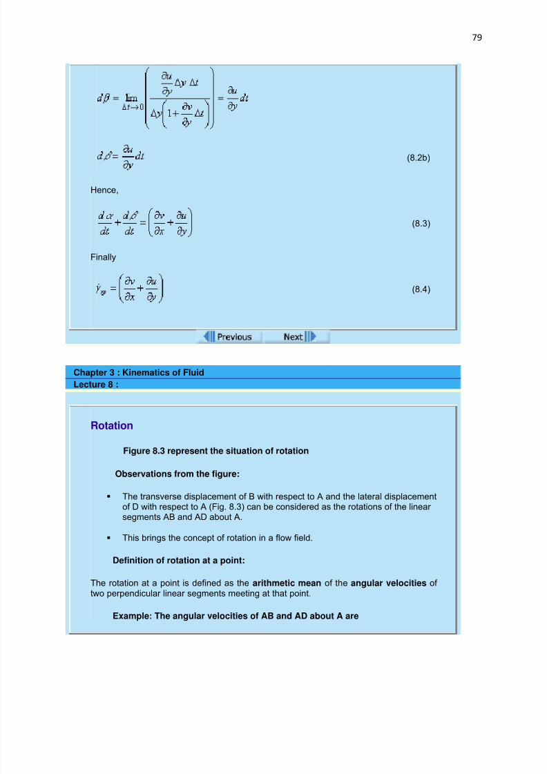
7/29/2019 FLUID MECHANICS LECTURE NOTES
http://slidepdf.com/reader/full/fluid-mechanics-lecture-notes 79/297
79
(8.2b)
Hence,
(8.3)
Finally
(8.4)
Chapter 3 : Kinematics of Fluid
Lecture 8 :
Rotation
Figure 8.3 represent the situation of rotation
Observations from the figure:
The transverse displacement of B with respect to A and the lateral displacementof D with respect to A (Fig. 8.3) can be considered as the rotations of the linear segments AB and AD about A.
This brings the concept of rotation in a flow field.
Definition of rotation at a point:
The rotation at a point is defined as the arithmetic mean of the angular velocities of two perpendicular linear segments meeting at that point.
Example: The angular velocities of AB and AD about A are

7/29/2019 FLUID MECHANICS LECTURE NOTES
http://slidepdf.com/reader/full/fluid-mechanics-lecture-notes 80/297
80
and respectively.
Considering the anticlockwise direction as positive, the rotation at A can be writtenas,
(8.5a)
or
(8.5b)
The suffix z in ω represents the rotation about z-axis.
When u = u (x, y) and v = v (x, y) the rotation and angular deformation of a fluid
element exist simultaneously.
Special case : Situation of pure Rotation
, and
Observation:
The linear segments AB and AD move with the same angular velocity (both inmagnitude and direction).
The included angle between them remains the same and no angular deformation takes place. This situation is known as pure rotation.
Chapter 3 : Kinematics of Fluid
Lecture 8 :
7/29/2019 FLUID MECHANICS LECTURE NOTES
http://slidepdf.com/reader/full/fluid-mechanics-lecture-notes 81/297
81
Vorticity
Definition: The vorticity Ω in its simplest form is defined as a vector which is equal totwo times the rotation vector
(8.6)
For an irrotational flow, vorticity components are zero.
Vortex line:
If tangent to an imaginary line at a point lying on it is in the direction of the Vorticityvector at that point , the line is a vortex line.
The general equation of the vortex line can be written as,
(8.6b)
In a rectangular cartesian cartesian coordinate system, it becomes
(8.6c)
where,
Vorticity components as vectors:
The vorticity is actually an anti symmetric tensor and its three distinct elementstransform like the components of a vector in cartesian coordinates.
This is the reason for which the vorticity components can be treated as vectors.
Existence of Flow
A fluid must obey the law of conservation of mass in course of its flow as it is amaterial body.
For a Velocity field to exist in a fluid continuum, the velocity components mustobey the mass conservation principle.

7/29/2019 FLUID MECHANICS LECTURE NOTES
http://slidepdf.com/reader/full/fluid-mechanics-lecture-notes 82/297
82
Velocity components which follow the mass conservation principle are said toconstitute a possible fluid flow
Velocity components violating this principle, are said to describe an impossibleflow.
The existence of a physically possible flow field is verified from the principle of conservation of mass.
The detailed discussion on this is deferred to the next chapter along with thediscussion on principles of conservation of momentum and energy.
End of Lecture 8!
To view the exercise problem, clicknext button or select from left-hand-side.
Module 2 :
Chapter 4 : Conservation Equations and Analysis of Finite Control Volume
The chapter contains
Lecture 9
System
Conservation of Mass
Lecture 10
Stream Function
Conservation of Momentum
7/29/2019 FLUID MECHANICS LECTURE NOTES
http://slidepdf.com/reader/full/fluid-mechanics-lecture-notes 83/297
83
Lecture 11
Analysis of Finite Control Volumes
Lecture 12
Application of Moment or Momentum Theorem
Euler's Equation
Lecture 13
Conservation Of Energy
Exercise Problem
Chapter 4 : Conservation Equations and Analysis of Finite Control Volume
Lecture 9 :

7/29/2019 FLUID MECHANICS LECTURE NOTES
http://slidepdf.com/reader/full/fluid-mechanics-lecture-notes 84/297
84
System
Definition
System: A quantity of matter in space which is analyzed during a problem.
Surroundings: Everything external to the system.
System Boundary: A separation present between system and surrounding.
Classification of the system boundary:-
Real solid boundary Imaginary boundary
The system boundary may be further classified as:-
Fixed boundary or Control Mass System Moving boundary or Control Volume System
The choice of boundary depends on the problem being analyzed.
Fig 9.1 System and Surroundings
Classification of Systems
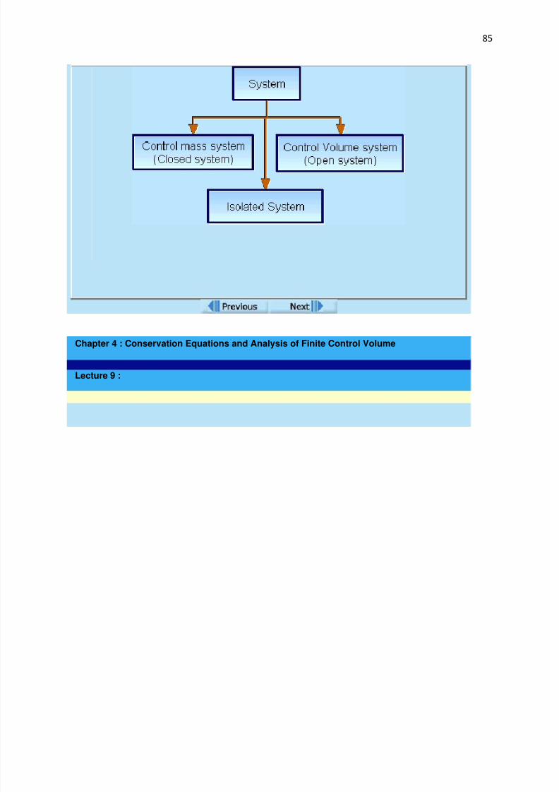
7/29/2019 FLUID MECHANICS LECTURE NOTES
http://slidepdf.com/reader/full/fluid-mechanics-lecture-notes 85/297
85
Chapter 4 : Conservation Equations and Analysis of Finite Control Volume
Lecture 9 :

7/29/2019 FLUID MECHANICS LECTURE NOTES
http://slidepdf.com/reader/full/fluid-mechanics-lecture-notes 86/297
86
Types of System
Control Mass System (Closed System)
1. Its a system of fixed mass with fixed identity.2. This type of system is usually referred to as "closed system".
3. There is no mass transfer across the system boundary.
4. Energy transfer may take place into or out of the system.
Click to play the Demonstration
Fig 9.2 A Control Mass System or Closed System
Control Volume System (Open System)
1. Its a system of fixed volume.2. This type of system is usually referred to as "open system” or a "control
volume" 3. Mass transfer can take place across a control volume.4. Energy transfer may also occur into or out of the system.5. A control volume can be seen as a fixed region across which mass and energy
transfers are studied.6. Control Surface- Its the boundary of a control volume across which the transfer
of both mass and energy takes place.7. The mass of a control volume (open system) may or may not be fixed.8. When the net influx of mass across the control surface equals zero then the
mass of the system is fixed and vice-versa.9. The identity of mass in a control volume always changes unlike the case for a
control mass system (closed system).10. Most of the engineering devices, in general, represent an open system or
control volume.
Example:-
Heat exchanger - Fluid enters and leaves the system continuously with thetransfer of heat across the system boundary.

7/29/2019 FLUID MECHANICS LECTURE NOTES
http://slidepdf.com/reader/full/fluid-mechanics-lecture-notes 87/297
87
Pump - A continuous flow of fluid takes place through the system with a transfer of mechanical energy from the surroundings to the system.
Click to play the Demonstration
Fig 9.3 A Control Volume System or Open System
Isolated System
1. Its a system of fixed mass with same identity and fixed energy.2. No interaction of mass or energy takes place between the system and the
surroundings.3. In more informal words an isolated system is like a closed shop amidst a busy
market.
Fig 9.4 An Isolated System
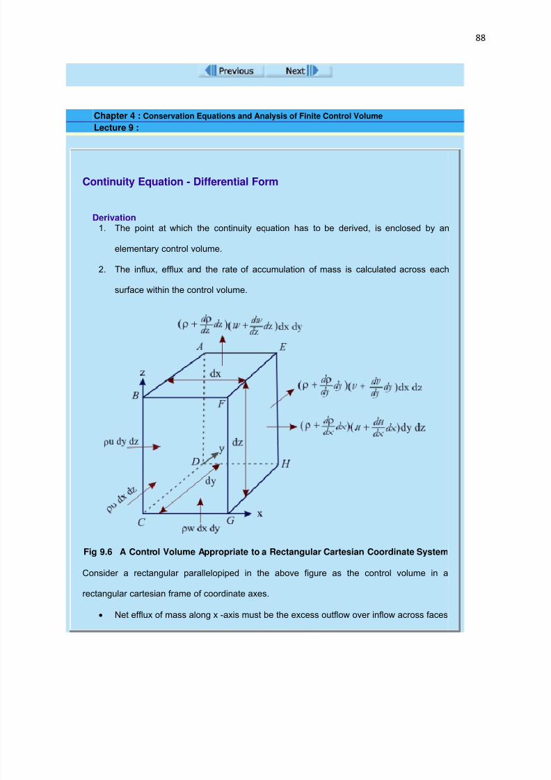
7/29/2019 FLUID MECHANICS LECTURE NOTES
http://slidepdf.com/reader/full/fluid-mechanics-lecture-notes 88/297
88
Chapter 4 : Conservation Equations and Analysis of Finite Control Volume
Lecture 9 :
Continuity Equation - Differential Form
Derivation 1. The point at which the continuity equation has to be derived, is enclosed by an
elementary control volume.
2. The influx, efflux and the rate of accumulation of mass is calculated across each
surface within the control volume.
Fig 9.6 A Control Volume Appropriate to a Rectangular Cartesian Coordinate System
Consider a rectangular parallelopiped in the above figure as the control volume in a
rectangular cartesian frame of coordinate axes.
Net efflux of mass along x -axis must be the excess outflow over inflow across faces

7/29/2019 FLUID MECHANICS LECTURE NOTES
http://slidepdf.com/reader/full/fluid-mechanics-lecture-notes 89/297
89
normal to x -axis.
Let the fluid enter across one of such faces ABCD with a velocity u and a densityρ.The velocity and density with which the fluid will leave the face EFGH will be
and respectively (neglecting the higher order terms in δx).
Therefore, the rate of mass entering the control volume through face ABCD = ρu dy dz .
The rate of mass leaving the control volume through face EFGH will be
(neglecting the higher order terms in dx)
Similarly influx and efflux take place in all y and z directions also.
Rate of accumulation for a point in a flow field
Using, Rate of influx = Rate of Accumulation + Rate of Efflux
Transferring everything to right side
(9.2)

7/29/2019 FLUID MECHANICS LECTURE NOTES
http://slidepdf.com/reader/full/fluid-mechanics-lecture-notes 90/297
90
This is the Equation of Continuity for a compressible fluid in a rectangular cartesiancoordinate system.
Chapter 4 : Conservation Equations and Analysis of Finite Control Volume
Lecture 9 :
Continuity Equation - Vector Form
The continuity equation can be written in a vector form as
or,(9.3)
where is the velocity of the point
In case of a steady flow,

7/29/2019 FLUID MECHANICS LECTURE NOTES
http://slidepdf.com/reader/full/fluid-mechanics-lecture-notes 91/297
91
Hence Eq. (9.3) becomes
(9.4)
In a rectangular cartesian coordinate system
(9.5)
Equation (9.4) or (9.5) represents the continuity equation for a steady
flow.
In case of an incompressible flow, ρ = constant
Hence,
Moreover
Therefore, the continuity equation for an incompressible flow becomes
(9.6)
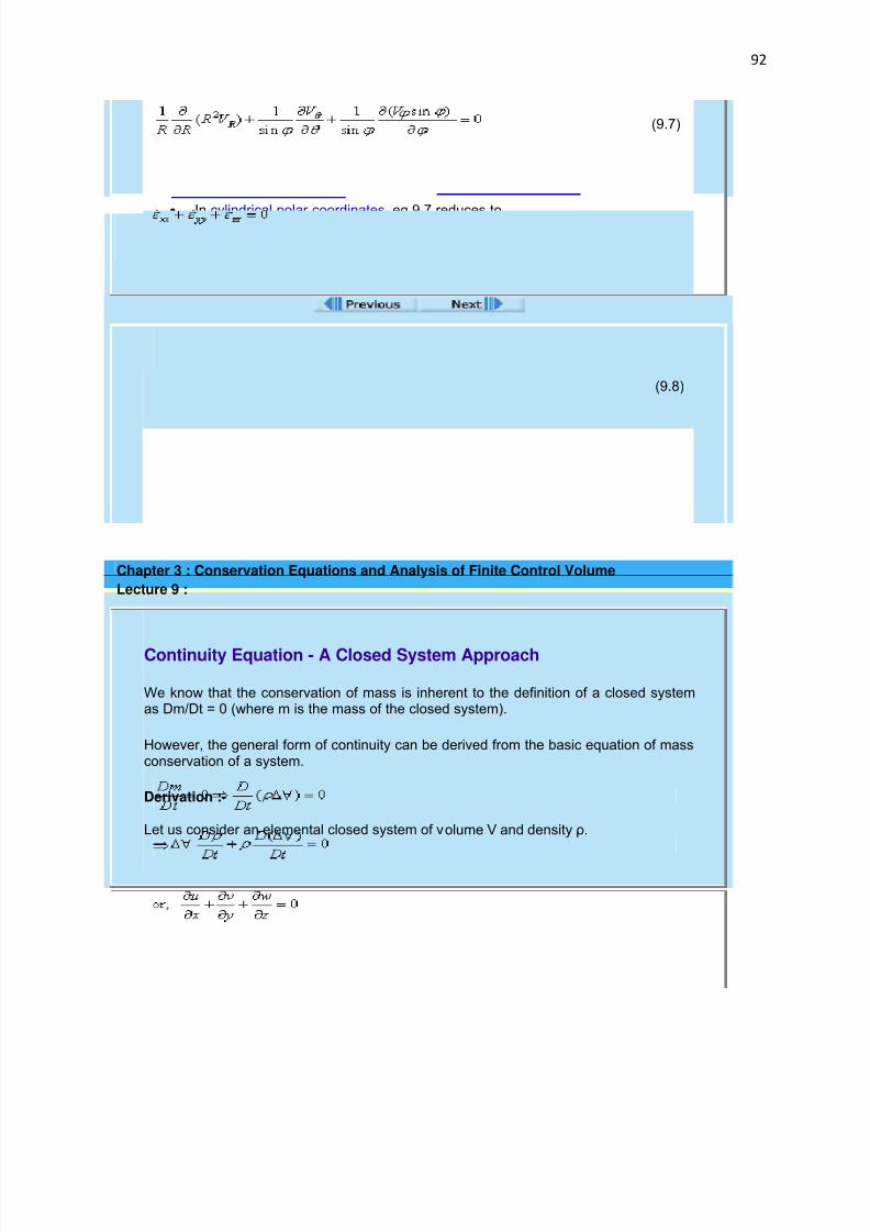
7/29/2019 FLUID MECHANICS LECTURE NOTES
http://slidepdf.com/reader/full/fluid-mechanics-lecture-notes 92/297
92
(9.7)
In cylindrical polar coordinates eq.9.7 reduces to
Eq. (9.7) can be written in terms of the strain rate components as
(9.8)
Chapter 3 : Conservation Equations and Analysis of Finite Control Volume
Lecture 9 :
Continuity Equation - A Closed System Approach
We know that the conservation of mass is inherent to the definition of a closed systemas Dm/Dt = 0 (where m is the mass of the closed system).
However, the general form of continuity can be derived from the basic equation of massconservation of a system.
Derivation :-
Let us consider an elemental closed system of volume V and density ρ.
7/29/2019 FLUID MECHANICS LECTURE NOTES
http://slidepdf.com/reader/full/fluid-mechanics-lecture-notes 93/297
93
Now (dilation per unit volume)
In vector notation we can write this as
The above equations are same as that formulated from Control Volume approach
End of Lecture 9!
To start next lecture click Next buttonor select from left-hand-side.
Chapter 4 : Conservation Equations and Analysis of Finite Control Volume
Lecture 10 :

7/29/2019 FLUID MECHANICS LECTURE NOTES
http://slidepdf.com/reader/full/fluid-mechanics-lecture-notes 94/297
94
Stream Function
Let us consider a two-dimensional incompressible flow parallel to the x - y plane in a rectangular cartesian coordinate system. The flow field in this case is defined by
u = u(x, y, t) v = v(x, y, t)
w = 0
The equation of continuity is
(10.1)
If a function ψ(x, y, t) is defined in the manner
(10.2a)
(10.2b)
so that it automatically satisfies the equation of continuity (Eq. (10.1)), then the functionis known as stream function.Note that for a steady flow, ψ is a function of two variables x and y only.
Constancy of ψ on a Streamline
Since ψ is a point function, it has a value at every point in the flow field. Thus a changein the stream function ψ can be written as
The equation of a streamline is given by
It follows that dψ = 0 on a streamline.This implies the value of ψ is constant along a streamline.Therefore, the equation of a streamline can be expressed in terms of stream function as
ψ(x, y) = constant (10.3)
Once the function ψ is known, streamline can be drawn by joining the samevalues of ψ in the flow field.
Stream function for an irrotational flow

7/29/2019 FLUID MECHANICS LECTURE NOTES
http://slidepdf.com/reader/full/fluid-mechanics-lecture-notes 95/297
95
In case of a two-dimensional irrotational flow
Conclusion drawn:For an irrotational flow, stream function satisfies the Laplace’sequation
Chapter 4 : Conservation Equations and Analysis of Finite Control Volume
Lecture 10 :
Physical Significance of Stream Funtion ψ
Figure 10.1 illustrates a two dimensional flow.
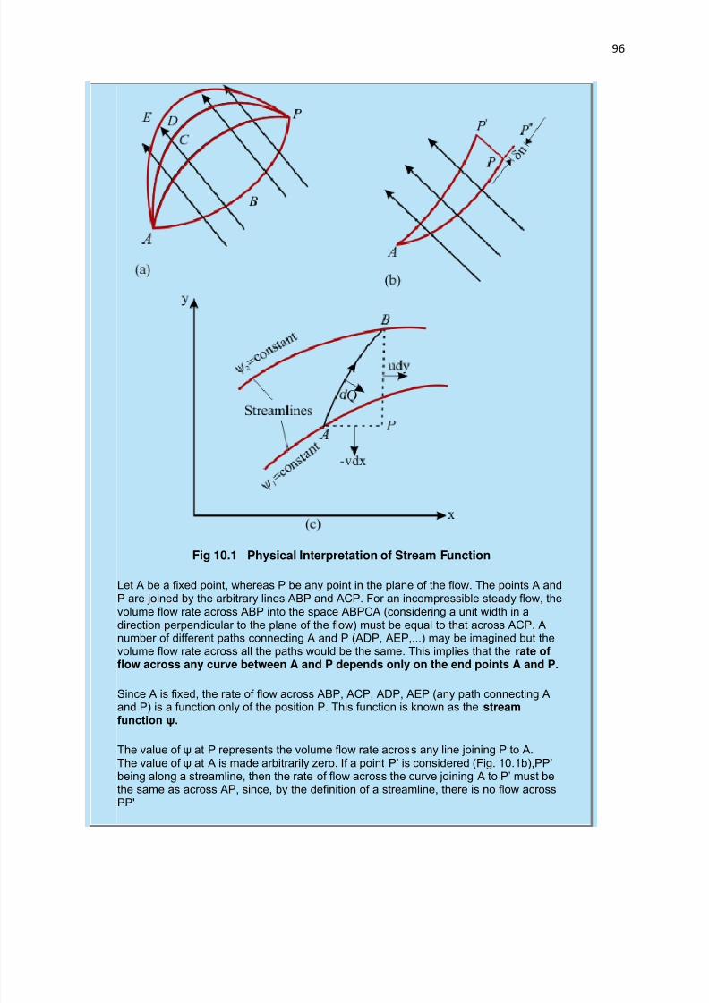
7/29/2019 FLUID MECHANICS LECTURE NOTES
http://slidepdf.com/reader/full/fluid-mechanics-lecture-notes 96/297
96
Fig 10.1 Physical Interpretation of Stream Function
Let A be a fixed point, whereas P be any point in the plane of the flow. The points A andP are joined by the arbitrary lines ABP and ACP. For an incompressible steady flow, thevolume flow rate across ABP into the space ABPCA (considering a unit width in adirection perpendicular to the plane of the flow) must be equal to that across ACP. Anumber of different paths connecting A and P (ADP, AEP,...) may be imagined but thevolume flow rate across all the paths would be the same. This implies that the rate offlow across any curve between A and P depends only on the end points A and P.
Since A is fixed, the rate of flow across ABP, ACP, ADP, AEP (any path connecting A
and P) is a function only of the position P. This function is known as the streamfunction ψ.
The value of ψ at P represents the volume flow rate across any line joining P to A.The value of ψ at A is made arbitrarily zero. If a point P’ is considered (Fig. 10.1b),PP’being along a streamline, then the rate of flow across the curve joining A to P’ must bethe same as across AP, since, by the definition of a streamline, there is no flow acrossPP'
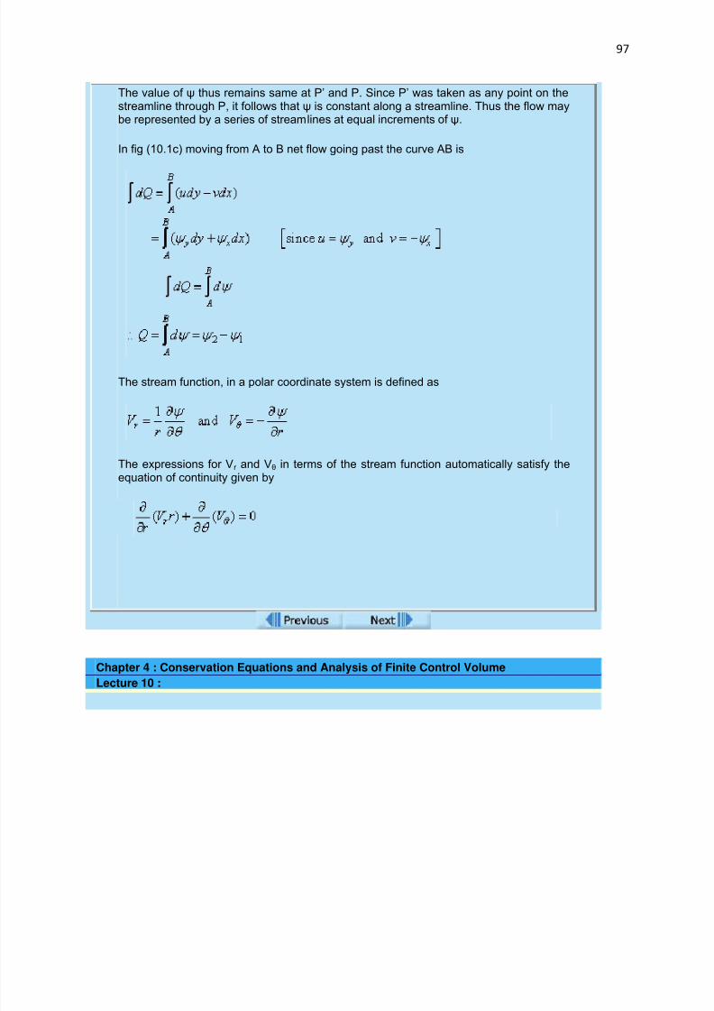
7/29/2019 FLUID MECHANICS LECTURE NOTES
http://slidepdf.com/reader/full/fluid-mechanics-lecture-notes 97/297
97
The value of ψ thus remains same at P’ and P. Since P’ was taken as any point on thestreamline through P, it follows that ψ is constant along a streamline. Thus the flow maybe represented by a series of stream lines at equal increments of ψ.
In fig (10.1c) moving from A to B net flow going past the curve AB is
The stream function, in a polar coordinate system is defined as
The expressions for Vr and Vθ in terms of the stream function automatically satisfy theequation of continuity given by
Chapter 4 : Conservation Equations and Analysis of Finite Control Volume
Lecture 10 :
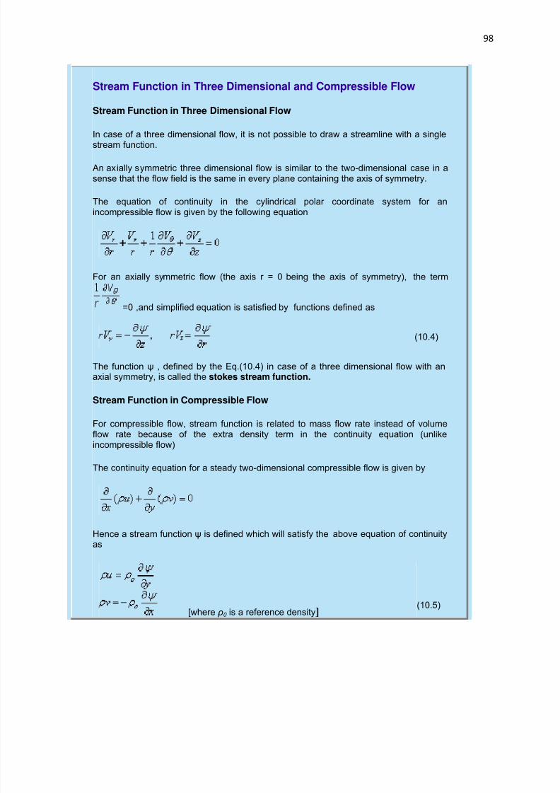
7/29/2019 FLUID MECHANICS LECTURE NOTES
http://slidepdf.com/reader/full/fluid-mechanics-lecture-notes 98/297
98
Stream Function in Three Dimensional and Compressible Flow
Stream Function in Three Dimensional Flow
In case of a three dimensional flow, it is not possible to draw a streamline with a singlestream function.
An axially symmetric three dimensional flow is similar to the two-dimensional case in asense that the flow field is the same in every plane containing the axis of symmetry.
The equation of continuity in the cylindrical polar coordinate system for anincompressible flow is given by the following equation
For an axially symmetric flow (the axis r = 0 being the axis of symmetry), the term
=0 ,and simplified equation is satisfied by functions defined as
(10.4)
The function ψ , defined by the Eq.(10.4) in case of a three dimensional flow with anaxial symmetry, is called the stokes stream function.
Stream Function in Compressible Flow
For compressible flow, stream function is related to mass flow rate instead of volumeflow rate because of the extra density term in the continuity equation (unlikeincompressible flow)
The continuity equation for a steady two-dimensional compressible flow is given by
Hence a stream function ψ is defined which will satisfy the above equation of continuityas
[where ρ0 is a reference density](10.5)

7/29/2019 FLUID MECHANICS LECTURE NOTES
http://slidepdf.com/reader/full/fluid-mechanics-lecture-notes 99/297
99
ρ0 is used to retain the unit of ψ same as that in the case of an incompressible flow.Physically, the difference in stream function between any two streamlines multiplied bythe reference density ρ0 will give the mass flow rate through the passage of unit width
formed by the streamlines.
Chapter 4 : Conservation Equations and Analysis of Finite Control Volume
Lecture 10 :
Continuity Equation: Integral Form
Let us consider a control volume bounded by the control surface S. The efflux of mass across the control surface S is given by
where is the velocity vector at an elemental area( which is treated as a vector byconsidering its positive direction along the normal drawn outward from the surface).
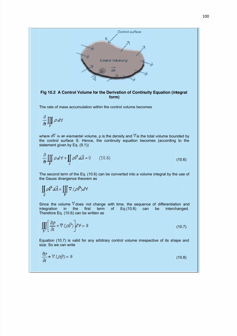
7/29/2019 FLUID MECHANICS LECTURE NOTES
http://slidepdf.com/reader/full/fluid-mechanics-lecture-notes 100/297
100
Fig 10.2 A Control Volume for the Derivation of Continuity Equation (integralform)
The rate of mass accumulation within the control volume becomes
where d is an elemental volume, ρ is the density and is the total volume bounded bythe control surface S. Hence, the continuity equation becomes (according to thestatement given by Eq. (9.1))
(10.6)
The second term of the Eq. (10.6) can be converted into a volume integral by the use of the Gauss divergence theorem as
Since the volume does not change with time, the sequence of differentiation andintegration in the first term of Eq.(10.6) can be interchanged.Therefore Eq. (10.6) can be written as
(10.7)
Equation (10.7) is valid for any arbitrary control volume irrespective of its shape andsize. So we can write
(10.8)

7/29/2019 FLUID MECHANICS LECTURE NOTES
http://slidepdf.com/reader/full/fluid-mechanics-lecture-notes 101/297
101
Chapter 4 : Conservation Equations and Analysis of Finite Control Volume
Lecture 10 :
Conservation of Momentum: Momentum Theorem
In Newtonian mechanics, the conservation of momentum is defined by Newton’s secondlaw of motion.
Newton’s Second Law of Motion
The rate of change of momentum of a body is proportional to the impressedaction and takes place in the direction of the impressed action.
If a force acts on the body ,linear momentum is implied.
If a torque (moment) acts on the body,angular momentum is implied.
Reynolds Transport Theorem
A study of fluid flow by the Eulerian approach requires a mathematical modeling for acontrol volume either in differential or in integral form. Therefore the physical statementsof the principle of conservation of mass, momentum and energy with reference to acontrol volume become necessary.
This is done by invoking a theorem known as the Reynolds transport theorem whichrelates the control volume concept with that of a control mass system in terms of ageneral property of the system.
Statement of Reynolds Transport Theorem
The theorem states that "the time rate of increase of property N within a control masssystem is equal to the time rate of increase of property N within the control volume plusthe net rate of efflux of the property N across the control surface”.
Equation of Reynolds Transport Theorem
After deriving Reynolds Transport Theorem according to the above statement we get
(10.9)

7/29/2019 FLUID MECHANICS LECTURE NOTES
http://slidepdf.com/reader/full/fluid-mechanics-lecture-notes 102/297
102
In this equation
N - flow property which is transported
η - intensive value of the flow property
Chapter 4 : Conservation Equations and Analysis of Finite Control Volume
Lecture 11 :
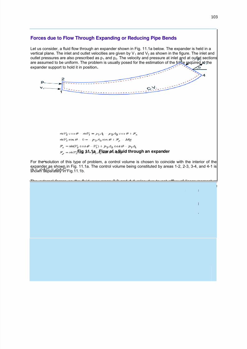
7/29/2019 FLUID MECHANICS LECTURE NOTES
http://slidepdf.com/reader/full/fluid-mechanics-lecture-notes 103/297
103
Forces due to Flow Through Expanding or Reducing Pipe Bends
Let us consider, a fluid flow through an expander shown in Fig. 11.1a below. The expander is held in avertical plane. The inlet and outlet velocities are given by V 1 and V2 as shown in the figure. The inlet andoutlet pressures are also prescribed as p1 and p2. The velocity and pressure at inlet and at outlet sections
are assumed to be uniform. The problem is usually posed for the estimation of the force required at theexpander support to hold it in position .
Fig 11.1a Flow of a fluid through an expander
For the solution of this type of problem, a control volume is chosen to coincide with the interior of theexpander as shown in Fig. 11.1a. The control volume being constituted by areas 1-2, 2-3, 3-4, and 4-1 isshown separately in Fig.11.1b.
The external forces on the fluid over areas 2-3 and 1-4 arise due to net efflux of linear momentumthrough the interior surface of the expander. Let these forces be F x and Fy. Since the control volume1234 is stationary and at a steady state, we apply Eq.(10.18d) and have for x and y components
(11.1a)
and (11.1b)
or, (11.2a)
and (11.2b)
where = mass flow rate through the expander. Analytically it can be expressed as
where A1 and A2 are the cross-sectional areas at inlet and outlet of the expander and the flow isconsidered to be incompressible.
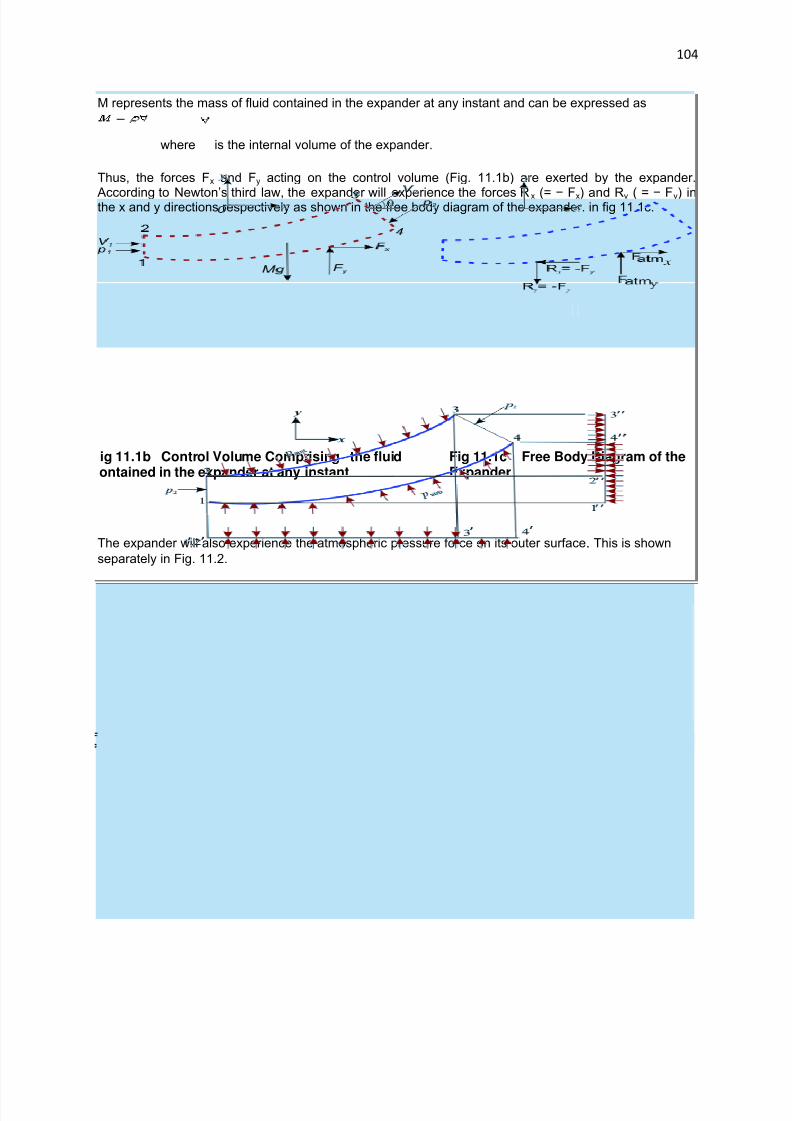
7/29/2019 FLUID MECHANICS LECTURE NOTES
http://slidepdf.com/reader/full/fluid-mechanics-lecture-notes 104/297
104
M represents the mass of fluid contained in the expander at any instant and can be expressed as
where is the internal volume of the expander.
Thus, the forces Fx and Fy acting on the control volume (Fig. 11.1b) are exerted by the expander.
According to Newton’s third law, the expander will experience the forces R x (= − Fx) and Ry ( = − Fy) inthe x and y directions respectively as shown in the free body diagram of the expander. in fig 11.1c.
ig 11.1b Control Volume Comprising the fluidontained in the expander at any instant
Fig 11.1c Free Body Diagram of theExpander
The expander will also experience the atmospheric pressure force on its outer surface. This is shown
separately in Fig. 11.2.
Fig 11.2 Effect of atmospheric pressure on the expander

7/29/2019 FLUID MECHANICS LECTURE NOTES
http://slidepdf.com/reader/full/fluid-mechanics-lecture-notes 105/297
105
From Fig.11.2 the net x and y components of the atmospheric pressure force on the expander can bewritten as
The net force on the expander is therefore,
(11.3a)
(11.3b)
or,
(11.4a)
(11.4b)
Note: At this stage that if Fx and Fy are calculated from the Eqs (11.2a) and (11.2b) with p 1 and p2 as thegauge pressures instead of the absolute ones the net forces on the expander Ex and Ey will respectivelybe equal to −Fx and −Fy.
Chapter 4 : Conservation Equations and Analysis of Finite Control Volume
Lecture 11 :
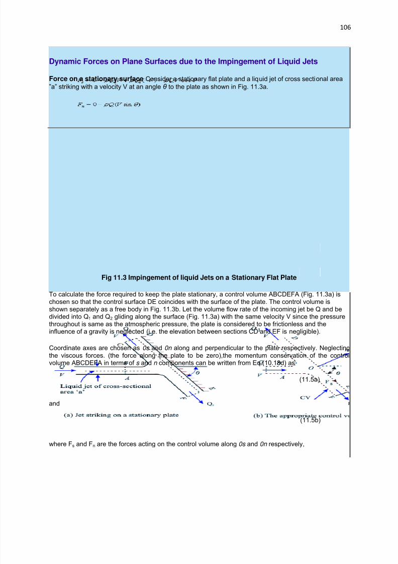
7/29/2019 FLUID MECHANICS LECTURE NOTES
http://slidepdf.com/reader/full/fluid-mechanics-lecture-notes 106/297
106
Dynamic Forces on Plane Surfaces due to the Impingement of Liquid Jets
Force on a stationary surface Consider a stationary flat plate and a liquid jet of cross sectional area
”a” striking with a velocity V at an angle θ to the plate as shown in Fig. 11.3a.
Fig 11.3 Impingement of liquid Jets on a Stationary Flat Plate
To calculate the force required to keep the plate stationary, a control volume ABCDEFA (Fig. 11.3a) ischosen so that the control surface DE coincides with the surface of the plate. The control volume isshown separately as a free body in Fig. 11.3b. Let the volume flow rate of the incoming jet be Q and bedivided into Q1 and Q2 gliding along the surface (Fig. 11.3a) with the same velocity V since the pressurethroughout is same as the atmospheric pressure, the plate is considered to be frictionless and theinfluence of a gravity is neglected (i.e. the elevation between sections CD and EF is negligible).
Coordinate axes are chosen as 0s and 0n along and perpendicular to the plate respectively. Neglectingthe viscous forces. (the force along the plate to be zero),the momentum conservation of the controlvolume ABCDEFA in terms of s and n components can be written from Eq.(10.18d) as
(11.5a)
and
(11.5b)
where Fs and Fn are the forces acting on the control volume along 0s and 0n respectively,
7/29/2019 FLUID MECHANICS LECTURE NOTES
http://slidepdf.com/reader/full/fluid-mechanics-lecture-notes 107/297
107
From continuity,
Q = Q1 + Q2 (11.6)
With the help of Eqs (11.5a) and (11.6), we can write
(11.7a)
(11.7b)
The net force acting on the control volume due to the change in momentum of the jet by the plate is F n along the direction "On ” and is given by the Eq. (11.7b) as
(11.7c)
Hence, according to Newton’s third law, the force acting on the plate is
(11.8)
If the cross-sectional area of the jet is ”a”, then the volume flow rate Q striking the plate can be written asQ = aV. Equation (11.8) then becomes
(11.9)
Let us solve another stationary vane problem
Chapter 4 : Conservation Equations and Analysis of Finite Control VolumeLecture 11 :

7/29/2019 FLUID MECHANICS LECTURE NOTES
http://slidepdf.com/reader/full/fluid-mechanics-lecture-notes 108/297
108
Force on a moving surface
Fig 11.5 Impingement of liquid jet on a moving flat plate
If the plate in the above problem moves with a uniform velocity u in the direction of jetvelocity V (Fig. 11.5). The volume of the liquid striking the plate per unit time will be
Q = a(V − u) (11.10)
Physically, when the plate recedes away from the jet it receives a less quantity of liquidper unit time than the actual mass flow rate of liquid delivered, say by any nozzle. Whenu = V, Q = 0 and when u > V, Q becomes negative. This implies physically that whenthe plate moves away from the jet with a velocity being equal to or greater than that of the jet, the jet can never strike the plate.
The control volume ABCDEFA in the case has to move with the velocity u of the plate.
Therefore we have to apply Eq. (10.18d) to calculate the forces acting on the controlvolume. Hence the velocities relative to the control volume will come into picture. Thevelocity of jet relative to the control volume at its inlet becomes VR1 = V − u
Since the pressure remains same throughout, the magnitudes of the relative velocitiesof liquid at outlets become equal to that at inlet, provided the friction between the plateand the liquid is neglected. Moreover, for a smooth shockless flow, the liquid has toglide along the plate and hence the direction of VR0, the relative velocity of the liquid atthe outlets, will be along the plate. The absolute velocities of the liquid at the outlets can

7/29/2019 FLUID MECHANICS LECTURE NOTES
http://slidepdf.com/reader/full/fluid-mechanics-lecture-notes 109/297
109
be found out by adding vectorially the plate velocity u and the relative velocity of the jetV - u with respect to the plate. This is shown by the velocity triangles at the outlets (Fig.11.5). Coordinate axes fixed to the control volume ABCDEFA are chosen as ”0s” and”0n” along and perpendicular to the plate respectively.
The force acting on the control volume along the direction ”0s ” will be zero for a
frictionless flow. The net force acting on the control volume will be along ”0n ” only. Tocalculate this force Fn, the momentum theorem with respect to the control volume ABCDEFA can be written as
Substituting Q from Eq (11.10),
Hence the force acting on the plate becomes
(11.11)
If the plate moves with a velocity u in a direction opposite to that of V (plate movingtowards the jet), the volume of liquid striking the plate per unit time will be Q = a(V + u)and, finally, the force acting on the plate would be
(11.12)
From the comparison of the Eq. (11.9) with Eqs (11.11) and (11.12), conclusion can bedrawn that for a given value of jet velocity V, the force exerted on a moving plate by theet is either greater or lower than that exerted on a stationary plate depending upon
whether the plate moves towards the jet or-away from it respectively.The power developed due to the motion of the plate can be written (in case of the platemoving in the same direction as that of the jet) as
P = F p . U
(11.13)
Chapter 4 : Conservation Equations and Analysis of Finite Control Volume
Lecture 11 :
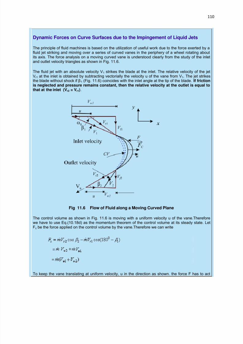
7/29/2019 FLUID MECHANICS LECTURE NOTES
http://slidepdf.com/reader/full/fluid-mechanics-lecture-notes 110/297
110
Dynamic Forces on Curve Surfaces due to the Impingement of Liquid Jets
The principle of fluid machines is based on the utilization of useful work due to the force exerted by afluid jet striking and moving over a series of curved vanes in the periphery of a wheel rotating aboutits axis. The force analysis on a moving curved vane is understood clearly from the study of the inlet
and outlet velocity triangles as shown in Fig. 11.6.
The fluid jet with an absolute velocity V1 strikes the blade at the inlet. The relative velocity of the jetVr1 at the inlet is obtained by subtracting vectorially the velocity u of the vane from V1. The jet strikesthe blade without shock if β1 (Fig. 11.6) coincides with the inlet angle at the tip of the blade. If frictionis neglected and pressure remains constant, then the relative velocity at the outlet is equal tothat at the inlet (Vr2 = Vr1).
Fig 11.6 Flow of Fluid along a Moving Curved Plane
The control volume as shown in Fig. 11.6 is moving with a uniform velocity u of the vane.Thereforewe have to use Eq.(10.18d) as the momentum theorem of the control volume at its steady state. LetFc be the force applied on the control volume by the vane.Therefore we can write
To keep the vane translating at uniform velocity, u in the direction as shown. the force F has to act

7/29/2019 FLUID MECHANICS LECTURE NOTES
http://slidepdf.com/reader/full/fluid-mechanics-lecture-notes 111/297
111
opposite to Fc Therefore,
(11.14)
From the outlet velocity triangle, it can be written
or,
or,
or, (11.15a)
Similarly from the inlet velocity triangle. it is possible to write
(11.15b)
Addition of Eqs (11.15a) and (11.15b) gives
Power developed is given by
(11.16)
The efficiency of the vane in developing power is given by
(11.17)
Chapter 4 : Conservation Equations and Analysis of Finite Control Volume
Lecture 11 :
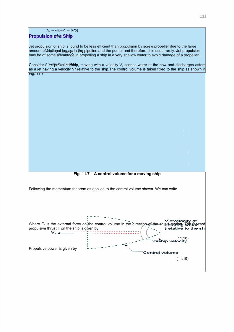
7/29/2019 FLUID MECHANICS LECTURE NOTES
http://slidepdf.com/reader/full/fluid-mechanics-lecture-notes 112/297
112
Propulsion of a Ship
Jet propulsion of ship is found to be less efficient than propulsion by screw propeller due to the largeamount of frictional losses in the pipeline and the pump, and therefore, it is used rarely. Jet propulsionmay be of some advantage in propelling a ship in a very shallow water to avoid damage of a propeller.
Consider a jet propelled ship, moving with a velocity V, scoops water at the bow and discharges asternas a jet having a velocity Vr relative to the ship.The control volume is taken fixed to the ship as shown inFig. 11.7.
Fig 11.7 A control volume for a moving ship
Following the momentum theorem as applied to the control volume shown. We can write
Where Fc is the external force on the control volume in the direction of the ship’s motion. The forwardpropulsive thrust F on the ship is given by
(11.18)
Propulsive power is given by
(11.19)
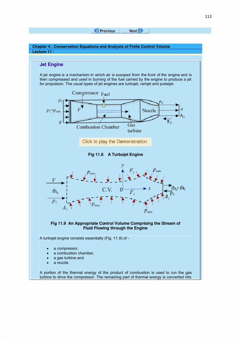
7/29/2019 FLUID MECHANICS LECTURE NOTES
http://slidepdf.com/reader/full/fluid-mechanics-lecture-notes 113/297
113
Chapter 4 : Conservation Equations and Analysis of Finite Control Volume
Lecture 11 :
Jet Engine
A jet engine is a mechanism in which air is scooped from the front of the engine and isthen compressed and used in burning of the fuel carried by the engine to produce a jetfor propulsion. The usual types of jet engines are turbojet, ramjet and pulsejet.
Fig 11.8 A Turbojet Engine
Fig 11.9 An Appropriate Control Volume Comprising the Stream ofFluid Flowing through the Engine
A turbojet engine consists essentially (Fig. 11.8) of -
a compressor,
a combustion chamber,
a gas turbine and
a nozzle.
A portion of the thermal energy of the product of combustion is used to run the gasturbine to drive the compressor. The remaining part of thermal energy is converted into

7/29/2019 FLUID MECHANICS LECTURE NOTES
http://slidepdf.com/reader/full/fluid-mechanics-lecture-notes 114/297
114
kinetic energy of the jet by a nozzle. At high speed fiight, jet engines are advantageoussince a propeller has to rotate at high speed to create a large thrust. This will result inexcessive blade stress and a decrease in the efficiency for blade tip speeds near andabove sonic level. In a jet propelled aircraft, the spent gases are ejected to thesurroundings at high velocity usually equal to or greater than the velocity of sound in thefluid at that state.
In many cases, depending upon the range of fight speeds, the jet is discharged with avelocity equal to sonic velocity in the medium and the pressure at discharge does notfall immediately to the ambient pressure. In these cases, the discharge pressure p2 atthe nozzle exit becomes higher than the ambient pressure patm. Under the situation of uniform velocity of the aircraft, we have to use Eg. (10.18d) as the momentum theoremfor the control volume as shown in Fig. 11.9 and can write
where, F x is the force acting on the control volume along the direction of the coordinateaxis ”OX” fixed to the control volume, V is the velocity of the aircraft, u is the relative
velocity of the exit jet with respect to the aircraft, and are the mass flow rate of
air, and mass burning rate of fuel respectively. Usually is very less compared to
usually varies from 0.01 to 0.02 in practice).
The propulsive thrust on the aircraft can be written as
(11.20)
The terms in the bracket are always positive. Hence, the negative sign in F T representsthat it acts in a direction opposite to ox, i.e. in the direction of the motion of the jetengine. The propulsive power is given by
(11.21)
Chapter 4 : Conservation Equations and Analysis of Finite Control Volume
Lecture 11 :

7/29/2019 FLUID MECHANICS LECTURE NOTES
http://slidepdf.com/reader/full/fluid-mechanics-lecture-notes 115/297
115
Non-inertial Control Volume
Rocket engine
Rocket engine works on the principle of jet propulsion.
The gases constituting the jet are produced by the combustion of a fuel andappropriate oxidant carried by the engine. Therefore, no air is required fromoutside and a rocket can operate satisfactorily in a vacuum.
A large quantity of oxidant has to be carried by the rocket for its operation to beindependent of the atmosphere.
At the start of journey, the fuel and oxidant together form a large portion of thetotal load carried by the rocket.
Work done in raising the fuel and oxidant to a great height before they are burnt
is wasted.
Therefore, to achieve the efficient use of the materials, the rocket is acceleratedto a high velocity in a short distance at the start. This period of rocketacceleration is of practical interest.
Fig 11.10 A Control Volume for a Rocket Engine
Let be the rate at which spent gases are discharged from the rocket with a velocity
u relative to the rocket (Fig. 11.10) Both and u are assumed to be constant.
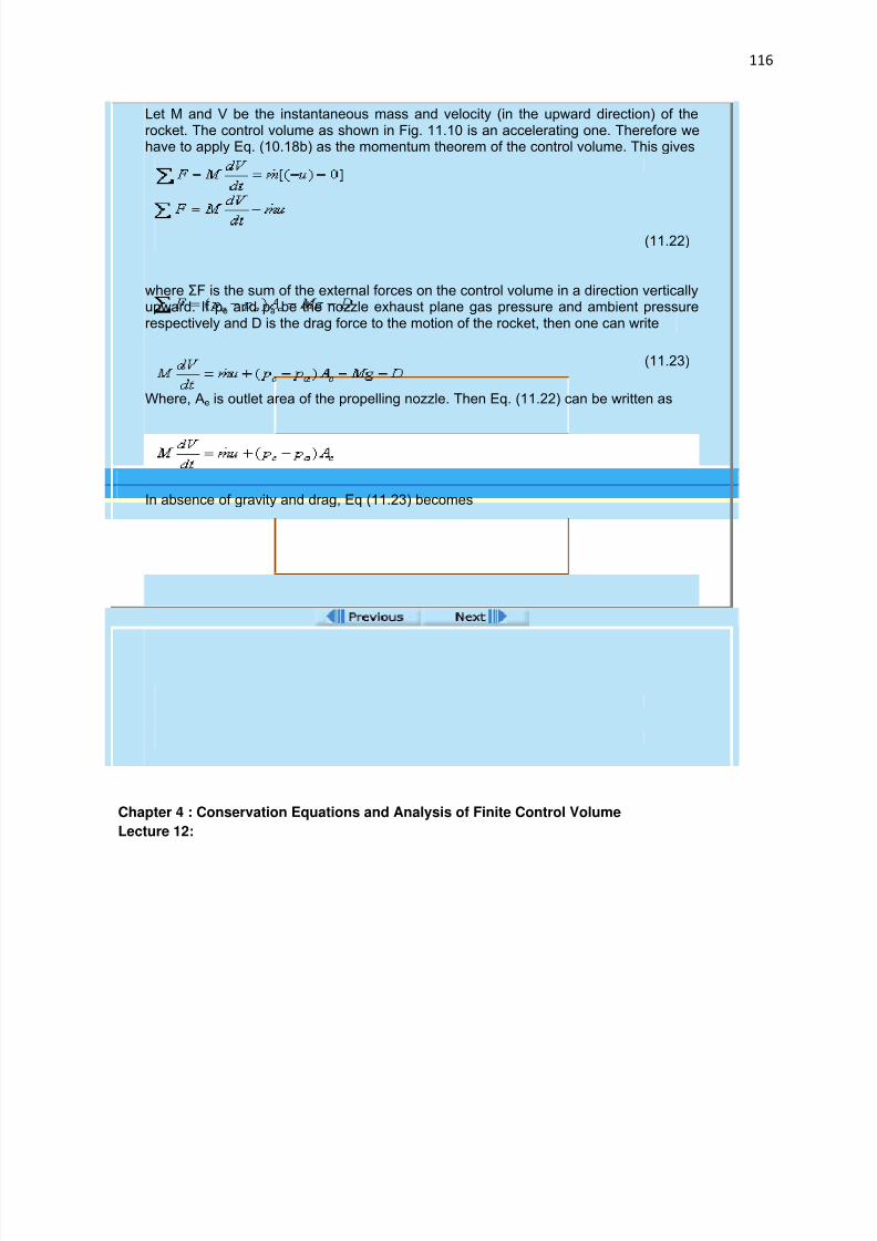
7/29/2019 FLUID MECHANICS LECTURE NOTES
http://slidepdf.com/reader/full/fluid-mechanics-lecture-notes 116/297
116
Let M and V be the instantaneous mass and velocity (in the upward direction) of therocket. The control volume as shown in Fig. 11.10 is an accelerating one. Therefore wehave to apply Eq. (10.18b) as the momentum theorem of the control volume. This gives
(11.22)
where ΣF is the sum of the external forces on the control volume in a direction verticallyupward. If pe and pa be the nozzle exhaust plane gas pressure and ambient pressurerespectively and D is the drag force to the motion of the rocket, then one can write
(11.23)
Where, Ae is outlet area of the propelling nozzle. Then Eq. (11.22) can be written as
In absence of gravity and drag, Eq (11.23) becomes
End of Lecture 11!
To start next lecture click next button orselect from left-hand-side.
Chapter 4 : Conservation Equations and Analysis of Finite Control Volume
Lecture 12:
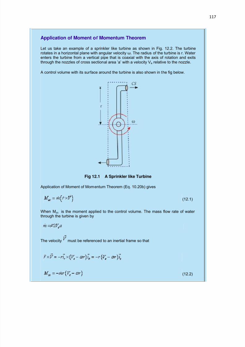
7/29/2019 FLUID MECHANICS LECTURE NOTES
http://slidepdf.com/reader/full/fluid-mechanics-lecture-notes 117/297
117
Application of Moment of Momentum Theorem
Let us take an example of a sprinkler like turbine as shown in Fig. 12.2. The turbinerotates in a horizontal plane with angular velocity ω. The radius of the turbine is r. Water enters the turbine from a vertical pipe that is coaxial with the axis of rotation and exits
through the nozzles of cross sectional area ’a’ with a velocity Ve relative to the nozzle.
A control volume with its surface around the turbine is also shown in the fig below.
Fig 12.1 A Sprinkler like Turbine
Application of Moment of Momentum Theorem (Eq. 10.20b) gives
(12.1)
When Mzc is the moment applied to the control volume. The mass flow rate of water through the turbine is given by
The velocity must be referenced to an inertial frame so that
(12.2)
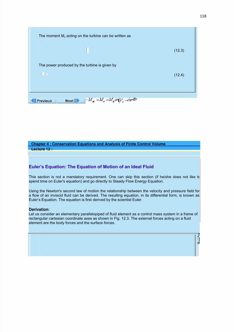
7/29/2019 FLUID MECHANICS LECTURE NOTES
http://slidepdf.com/reader/full/fluid-mechanics-lecture-notes 118/297
118
The moment Mz acting on the turbine can be written as
(12.3)
The power produced by the turbine is given by
(12.4)
Chapter 4 : Conservation Equations and Analysis of Finite Control Volume
Lecture 12 :
Euler’s Equation: The Equation of Motion of an Ideal Fluid
This section is not a mandatory requirement. One can skip this section (if he/she does not like tospend time on Euler's equation) and go directly to Steady Flow Energy Equation.
Using the Newton's second law of motion the relationship between the velocity and pressure field for a flow of an inviscid fluid can be derived. The resulting equation, in its differential form, is known asEuler’s Equation. The equation is first derived by the scientist Euler.
Derivation: Let us consider an elementary parallelopiped of fluid element as a control mass system in a frame of rectangular cartesian coordinate axes as shown in Fig. 12.3. The external forces acting on a fluidelement are the body forces and the surface forces.
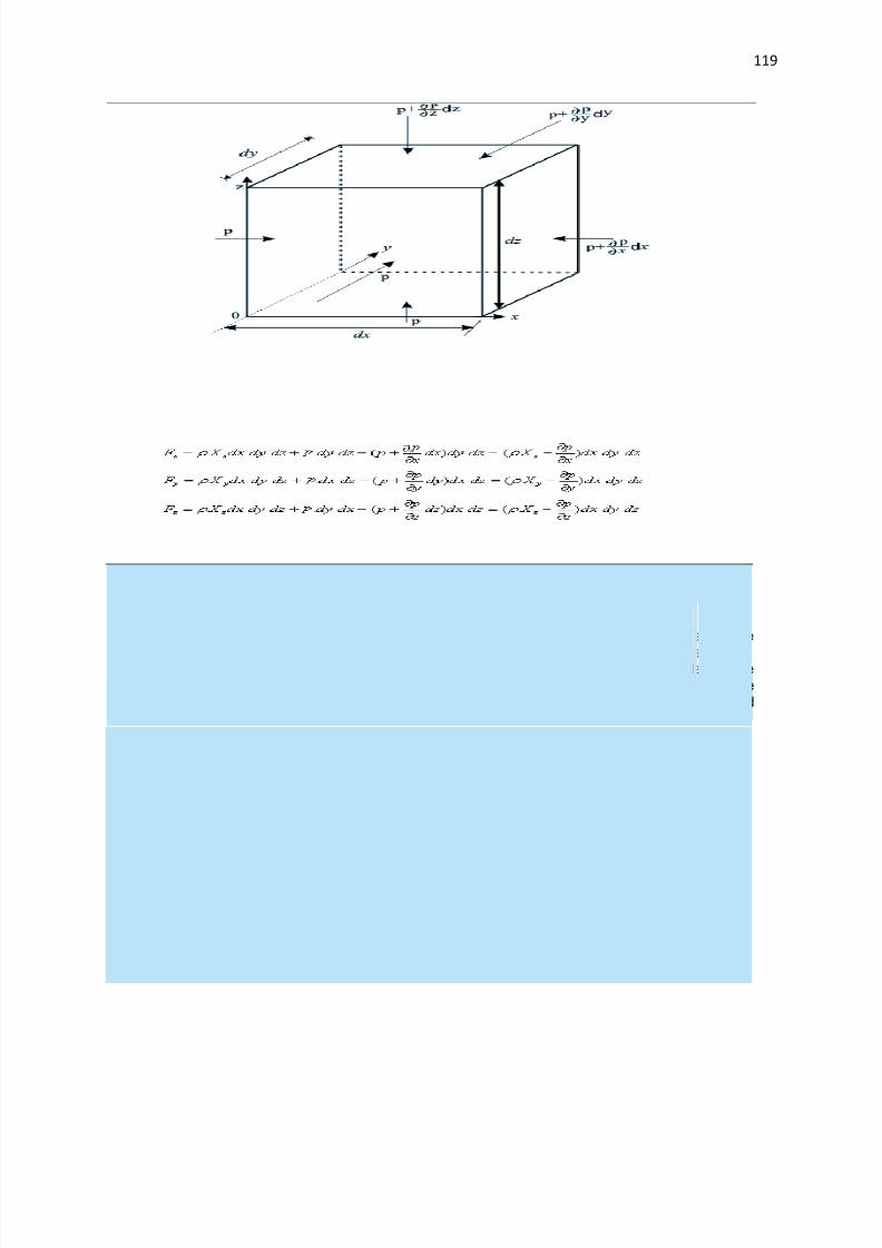
7/29/2019 FLUID MECHANICS LECTURE NOTES
http://slidepdf.com/reader/full/fluid-mechanics-lecture-notes 119/297
119
Fig 12.2 A Fluid Element appropriate to a Cartesian Coordinate Systemused for the derivation of Euler's Equation
Let Xx, Xy, Xz be the components of body forces acting per unit mass of the fluid element along the
coordinate axes x, y and z respectively. The body forces arise due to external force fields like gravity,electromagnetic field, etc., and therefore, the detailed description of Xx, Xy and Xz are provided by thelaws of physics describing the force fields. The surface forces for an inviscid fluid will be the pressureforces acting on different surfaces as shown in Fig. 12.3. Therefore, the net forces acting on the fluidelement along x, y and z directions can be written as
Since each component of the force can be expressed as the rate of change of momentum in therespective directions, we have

7/29/2019 FLUID MECHANICS LECTURE NOTES
http://slidepdf.com/reader/full/fluid-mechanics-lecture-notes 120/297
120
(12.5a)
(12.5b)
(12.5c)
s the mass of a control mass system does not change with time, is constant with time andcan be taken common. Therefore we can write Eqs (12.5a to 12.5c) as
(12.6a)
(12.6b)
(12.6c)
Expanding the material accelerations in Eqs (12.6a) to (12.6c) in terms of their respective temporaland convective components, we get
(12.7a)
(12.7b)
(12.7c)
The Eqs (12.7a, 12.7b, 12.7c) are valid for both incompressible and compressible flow. By putting u =v = w = 0, as a special case, one can obtain the equation of hydrostatics .Equations (12.7a), (12.7b), (12.7c) can be put into a single vector form as
(12.7d)
(12.7e)
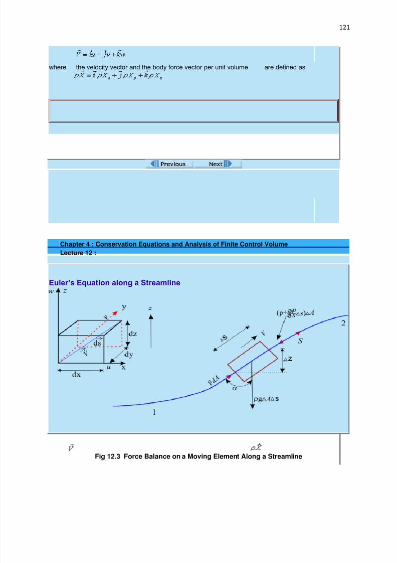
7/29/2019 FLUID MECHANICS LECTURE NOTES
http://slidepdf.com/reader/full/fluid-mechanics-lecture-notes 121/297
121
where the velocity vector and the body force vector per unit volume are defined as
Equation (12.7d) or (12.7e) is the well known Euler’s equation in vector form,while Eqs (12.7a) to (12.7c) describe the Euler’s equations in a rectangular Cartesian coordinatesystem.
Chapter 4 : Conservation Equations and Analysis of Finite Control Volume
Lecture 12 :
Euler’s Equation along a Streamline
Fig 12.3 Force Balance on a Moving Element Along a Streamline

7/29/2019 FLUID MECHANICS LECTURE NOTES
http://slidepdf.com/reader/full/fluid-mechanics-lecture-notes 122/297
122
Derivation Euler’s equation along a streamline is derived by applying Newton’s second law of motion to a fluidelement moving along a streamline. Considering gravity as the only body force component actingvertically downward (Fig. 12.3), the net external force acting on the fluid element along the directions canbe written as
(12.8)
where ∆A is the cross-sectional area of the fluid element. By the application of Newton’s second law of
motion in s direction, we get
(12.9)
From geometry we get
Hence, the final form of Eq. (12.9) becomes
(12.10)
Equation (12.10) is the Euler’s equation along a streamline.
Let us consider along the streamline so that
Again, we can write from Fig. 12.3
The equation of a streamline is given by
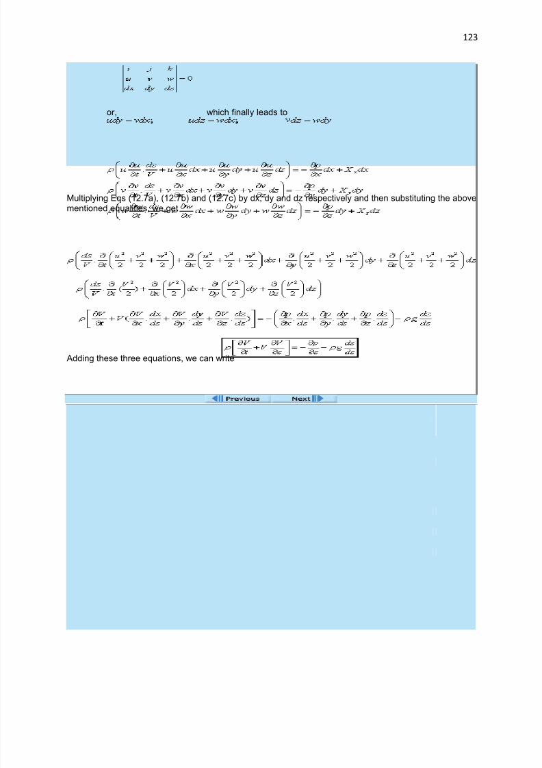
7/29/2019 FLUID MECHANICS LECTURE NOTES
http://slidepdf.com/reader/full/fluid-mechanics-lecture-notes 123/297
123
or, which finally leads to
Multiplying Eqs (12.7a), (12.7b) and (12.7c) by dx, dy and dz respectively and then substituting the abovementioned equalities, we get
Adding these three equations, we can write
=
=
Hence,
This is the more popular form of Euler's equation because the velocity vector in a flow field is alwaysdirected along the streamline.
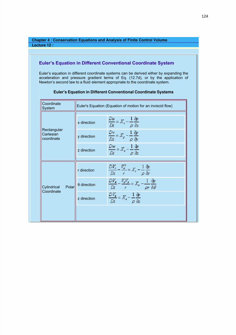
7/29/2019 FLUID MECHANICS LECTURE NOTES
http://slidepdf.com/reader/full/fluid-mechanics-lecture-notes 124/297
124
Chapter 4 : Conservation Equations and Analysis of Finite Control Volume
Lecture 12 :
Euler’s Equation in Different Conventional Coordinate System
Euler’s equation in different coordinate systems can be derived either by expanding theacceleration and pressure gradient terms of Eq. (12.7d), or by the application of Newton’s second law to a fluid element appropriate to the coordinate system.
Euler's Equation in Different Conventional Coordinate Systems
CoordinateSystem
Euler's Equation (Equation of motion for an inviscid flow)
Rectangular Cartesiancoordinate
x direction
y direction
z direction
Cylindrical Polar Coordinate
r direction
θ direction
z direction

7/29/2019 FLUID MECHANICS LECTURE NOTES
http://slidepdf.com/reader/full/fluid-mechanics-lecture-notes 125/297
125
Spherical Polar Coordinate
R direction
θ direction
φ direction
Chapter 4 : Conservation Equations and Analysis of Finite Control Volume
Lecture 12 :
A Control Volume Approach for the Derivation of Euler’s Equation
Euler’s equations of motion can also be derived by the use of the momentum theorem for a controlvolume.
Derivation In a fixed x, y, z axes (the rectangular cartesian coordinate system), the parallelopiped which was takenearlier as a control mass system is now considered as a control volume (Fig. 12.4).
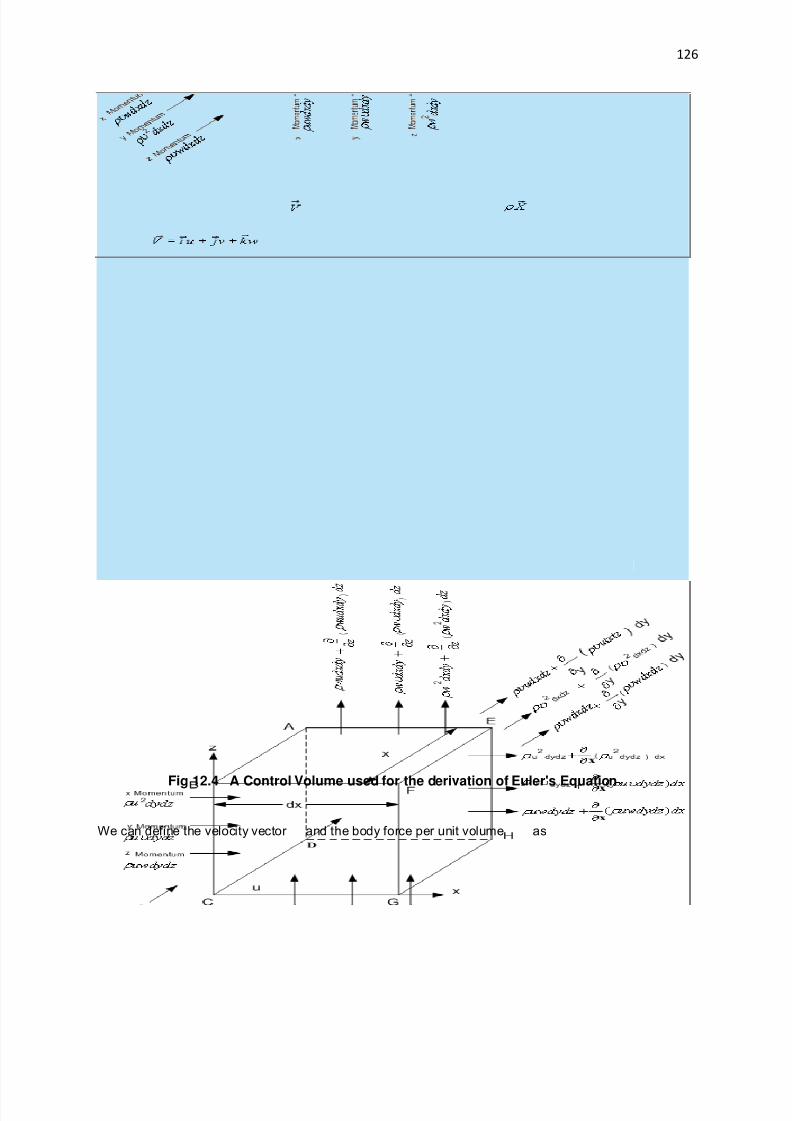
7/29/2019 FLUID MECHANICS LECTURE NOTES
http://slidepdf.com/reader/full/fluid-mechanics-lecture-notes 126/297
126
Fig 12.4 A Control Volume used for the derivation of Euler's Equation
We can define the velocity vector and the body force per unit volume as
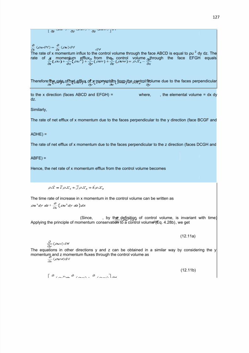
7/29/2019 FLUID MECHANICS LECTURE NOTES
http://slidepdf.com/reader/full/fluid-mechanics-lecture-notes 127/297
127
The rate of x momentum influx to the control volume through the face ABCD is equal to ρu2
dy dz. Therate of x momentum efflux from the control volume through the face EFGH equals
Therefore the rate of net efflux of x momentum from the control volume due to the faces perpendicular
to the x direction (faces ABCD and EFGH) = where, , the elemental volume = dx dydz.
Similarly,
The rate of net efflux of x momentum due to the faces perpendicular to the y direction (face BCGF and
ADHE) =
The rate of net efflux of x momentum due to the faces perpendicular to the z direction (faces DCGH and
ABFE) =
Hence, the net rate of x momentum efflux from the control volume becomes
The time rate of increase in x momentum in the control volume can be written as
(Since, , by the definition of control volume, is invariant with time) Applying the principle of momentum conservation to a control volume (Eq. 4.28b), we get
(12.11a)
The equations in other directions y and z can be obtained in a similar way by considering the ymomentum and z momentum fluxes through the control volume as
(12.11b)

7/29/2019 FLUID MECHANICS LECTURE NOTES
http://slidepdf.com/reader/full/fluid-mechanics-lecture-notes 128/297
128
(12.11c)
The typical form of Euler’s equations given by Eqs (12.11a), (12.11b) and (12.11c) are known as theconservative forms.
End of Lecture 12!
To start next lecture click next buttonor select from left-hand-side.
Chapter 4 : Conservation Equations and Analysis of Finite Control Volume
Lecture 13 :
Conservation of Energy
The principle of conservation of energy for a control mass system is described by thefirst law of thermodynamics
Heat Q added to a control mass system- the work done W by the control mass system =change in its internal energy E
The internal energy depends only upon the initial and final states of the system. It canbe written in the form of the equation as
(13.1a)
Equation (13.1a) can be expressed on the time rate basis as
(13.1b)
Where δQ and δW are the amount of heat added and work done respectively during atime interval of δt. To develop the analytical statement for the conservation of energy of a control volume, the Eq. (10.10) is used with N = E (the internal energy) and η = e (theinternal energy per unit mass) along with the Eq. (13.1b). This gives

7/29/2019 FLUID MECHANICS LECTURE NOTES
http://slidepdf.com/reader/full/fluid-mechanics-lecture-notes 129/297
129
(13.2)
The Eq. (13.2) is known as the general energy equation for a control volume.
The first term on the right hand side of the equation is the time rate of increase in theinternal energy within a control volume and the second term is the net rate of energyefflux from the control volume.
Different forms of energy associated with moving fluid elements comprising a controlvolume are -
1. Potential energyThe concept of potential energy in a fluid is essentially the same as that of a solid mass.The potential energy of a fluid element arises from its existence in a conservative bodyforce field. This field may be a magnetic, electrical, etc. In the absence of any of suchexternal force field, the earth’s gravitational effect is the only cause of potential energy.If a fluid mass m is stored in a reservoir and its C.G. is at a vertical distance z from an
arbitrary horizontal datum plane, then the potential energy is mgz and the potentialenergy per unit mass is gz. The arbitrary datum does not play a vital role since thedifference in potential energy, instead of its absolute value, is encountered in differentpractical purposes.
2. Kinetic Energy If a quantity of a fluid of mass m flows with a velocity V, being the same throughout itsmass, then the total kinetic energy is mV
2/2 and the kinetic energy per unit mass is V
2/2.
For a stream of real fluid, the velocities at different points will not be the same. If V is thelocal component of velocity along the direction of flow for a fluid flowing through an openchannel or closed conduit of cross-sectional area A, the total kinetic energy at anysection is evaluated by summing up the kinetic energy flowing through differential areasas
The average velocity at a cross-section in a flowing stream is defined on the basis of volumetric flow rate as,
The kinetic energy per unit mass of the fluid is usually expressed as where α
is known as the kinetic energy correction factor.Therefore, we can write

7/29/2019 FLUID MECHANICS LECTURE NOTES
http://slidepdf.com/reader/full/fluid-mechanics-lecture-notes 130/297
130
Hence,
(13.3a)
For an incompressible flow,
(13.3b)
3. Intermolecular EnergyThe intermolecular energy of a substance comprises the potential energy and kineticenergy of the molecules. The potential energy arises from intermolecular forces. For anideal gas, the potential energy is zero and the intermolecular energy is, therefore, due toonly the kinetic energy of molecules. The kinetic energy of the molecules of a substancedepends on its temperature.
4. Flow Work
Flow work is the work done by a fluid to move against pressure.For a flowing stream, a layer of fluid at any cross-section has to push the adjacentneighboring layer at its downstream in the direction of flow to make its way through and
thus does work on it. The amount of work done can be calculated by considering asmall amount of fluid mass A1 ρ1 dx to cross the surface AB from left to right (Fig. 13.1).The work done by this mass of fluid then becomes equal to p 1 A1 dx and thus the flowwork per unit mass can be expressed as
(where p1 is the pressure at section AB (Fig 13.1)
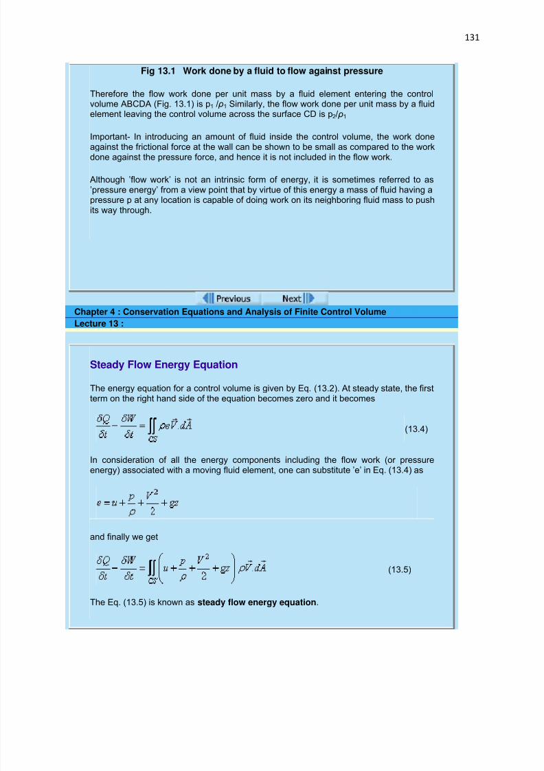
7/29/2019 FLUID MECHANICS LECTURE NOTES
http://slidepdf.com/reader/full/fluid-mechanics-lecture-notes 131/297
131
Fig 13.1 Work done by a fluid to flow against pressure
Therefore the flow work done per unit mass by a fluid element entering the controlvolume ABCDA (Fig. 13.1) is p1 / ρ1 Similarly, the flow work done per unit mass by a fluidelement leaving the control volume across the surface CD is p2/ ρ1
Important- In introducing an amount of fluid inside the control volume, the work doneagainst the frictional force at the wall can be shown to be small as compared to the workdone against the pressure force, and hence it is not included in the flow work.
Although ’flow work’ is not an intrinsic form of energy, it is sometimes referred to as’pressure energy’ from a view point that by virtue of this energy a mass of fluid having apressure p at any location is capable of doing work on its neighboring fluid mass to pushits way through.
Chapter 4 : Conservation Equations and Analysis of Finite Control Volume
Lecture 13 :
Steady Flow Energy Equation
The energy equation for a control volume is given by Eq. (13.2). At steady state, the firstterm on the right hand side of the equation becomes zero and it becomes
(13.4)
In consideration of all the energy components including the flow work (or pressureenergy) associated with a moving fluid element, one can substitute ’e’ in Eq. (13.4) as
and finally we get
(13.5)
The Eq. (13.5) is known as steady flow energy equation.
7/29/2019 FLUID MECHANICS LECTURE NOTES
http://slidepdf.com/reader/full/fluid-mechanics-lecture-notes 132/297
132
Chapter 4 : Conservation Equations and Analysis of Finite Control Volume
Lecture 13 :
Bernoulli's Equation
Energy Equation of an ideal Flow along a Streamline
Euler’s equation (the equation of motion of an inviscid fluid) along a stream line for asteady flow with gravity as the only body force can be written as
(13.6)
Application of a force through a distance ds along the streamline would physically implywork interaction. Therefore an equation for conservation of energy along a streamlinecan be obtained by integrating the Eq. (13.6) with respect to ds as
(13.7)
Where C is a constant along a streamline. In case of an incompressible flow, Eq. (13.7)can be written as
(13.8)
The Eqs (13.7) and (13.8) are based on the assumption that no work or heat interactionbetween a fluid element and the surrounding takes place. The first term of the Eq. (13.8)represents the flow work per unit mass, the second term represents the kinetic energyper unit mass and the third term represents the potential energy per unit mass.Therefore the sum of three terms in the left hand side of Eq. (13.8) can be consideredas the total mechanical energy per unit mass which remains constant along astreamline for a steady inviscid and incompressible flow of fluid. Hence the Eq. (13.8) isalso known as Mechanical energy equation.
This equation was developed first by Daniel Bernoulli in 1738 and is therefore referredto as Bernoulli’s equation. Each term in the Eq. (13.8) has the dimension of energy per unit mass. The equation can also be expressed in terms of energy per unit weight as
(13.9)

7/29/2019 FLUID MECHANICS LECTURE NOTES
http://slidepdf.com/reader/full/fluid-mechanics-lecture-notes 133/297
133
In a fluid flow, the energy per unit weight is termed as head. Accordingly, equation 13.9can be interpreted as
Pressure head + Velocity head + Potential head =Total head (total energy per unitweight).
Bernoulli's Equation with Head Loss
The derivation of mechanical energy equation for a real fluid depends much on theinformation about the frictional work done by a moving fluid element and is excludedfrom the scope of the book. However, in many practical situations, problems related toreal fluids can be analysed with the help of a modified form of Bernoulli’s equation as
(13.10)
where, hf
represents the frictional work done (the work done against the fluid friction)per unit weight of a fluid element while moving from a station 1 to 2 along a streamlinein the direction of flow. The term hf is usually referred to as head loss between 1 and 2,since it amounts to the loss in total mechanical energy per unit weight between points 1and 2 on a streamline due to the effect of fluid friction or viscosity. It physically signifiesthat the difference in the total mechanical energy between stations 1 and 2 is dissipatedinto intermolecular or thermal energy and is expressed as loss of head h f in Eq. (13.10).The term head loss, is conventionally symbolized as h L instead of hf in dealing withpractical problems. For an inviscid flow hL = 0, and the total mechanical energy isconstant along a streamline.
End of Lecture 13!
To view the exercise problem, clicknext button or select from left-hand-side.
\

7/29/2019 FLUID MECHANICS LECTURE NOTES
http://slidepdf.com/reader/full/fluid-mechanics-lecture-notes 134/297
134
Module 3 :
Chapter 5 : Equations of Motion and Mechanical Energy
Objectives
Lecture 14
Bernoulli's Equation In Irrotational Flow
Plane Circular Vortex Flows
Free Vortex Flows
Forced Vortex FlowsLosses Due to Geometric Changes
Lecture 15
Measurement Of Flow Rate Through Pipe
Lecture 16
Concept of Static Pressure
Concept of Stagnation Pressure
Flow through Orifices and Mouthpieces
Exercise Problem

7/29/2019 FLUID MECHANICS LECTURE NOTES
http://slidepdf.com/reader/full/fluid-mechanics-lecture-notes 135/297
7/29/2019 FLUID MECHANICS LECTURE NOTES
http://slidepdf.com/reader/full/fluid-mechanics-lecture-notes 136/297
136
(14.1)
The steady state Euler's equation can be written as
(14.2a)
(14.2b)
We consider the y-axis to be vertical and directed positive upward. From the condition
of irrotationality given by the Eq. (14.1), we substitute in place of in the Eq.
14.2a and in place of in the Eq. 14.2b. This results in
(14.3a)
(14.3b)
Now multiplying Eq.(14.3a) by 'dx' and Eq.(14.3b) by 'dy' and then adding these twoequations we have
(14.4)
The Eq. (14.4) can be physically interpreted as the equation of conservation of energyfor an arbitrary displacement
. Since, u, v and p are functions of x and y, we can write
(14.5a)
(14.5b)
7/29/2019 FLUID MECHANICS LECTURE NOTES
http://slidepdf.com/reader/full/fluid-mechanics-lecture-notes 137/297
137
(14.5c)
With the help of Eqs (14.5a), (14.5b), and (14.5c), the Eq. (14.4) can be written as
(14.6)
The integration of Eq. 14.6 results in
(14.7a)
For an incompressible flow,
(14.7b)
The constant C in Eqs (14.7a) and (14.7b) has the same value in the entire flow field,since no restriction was made in the choice of dr which was considered as an arbitrarydisplacement in evaluating the work.
Note: In deriving Eq. (13.8) the displacement ds was considered along a streamline.Therefore, the total mechanical energy remains constant everywhere in an inviscid andirrotational flow, while it is constant only along a streamline for an inviscid but rotational
flow.
The equation of motion for the flow of an inviscid fluid can be written in a vector form as

7/29/2019 FLUID MECHANICS LECTURE NOTES
http://slidepdf.com/reader/full/fluid-mechanics-lecture-notes 138/297
138
where is the body force vector per unit mass
Chapter 5 : Equations of Motion and Mechanical Energy
Lecture 14 :
Plane Circular Vortex Flows
Plane circular vortex flows are defined as flows where streamlines areconcentric circles. Therefore, with respect to a polar coordinate system with thecentre of the circles as the origin or pole, the velocity field can be described as
where Vθ and Vr are the tangential and radial component of velocity respectively.
The equation of continuity for a two dimensional incompressible flow in a polar coordinate system is
which for a plane circular vortex flow gives i.e. Vθ is not a function of θ. Hence,Vθ is a function of r only.
We can write for the variation of total mechanical energy with radius as
(14.8)
Click to see the Derivation
Free Vortex Flows
Free vortex flows are the plane circular vortex flows where the total mechanical
7/29/2019 FLUID MECHANICS LECTURE NOTES
http://slidepdf.com/reader/full/fluid-mechanics-lecture-notes 139/297
139
energy remains constant in the entire flow field. There is neither any additionnor any destruction of energy in the flow field.
Therefore, the total mechanical energy does not vary from streamline tostreamline. Hence from Eq. (14.8), we have,
or, (14.9)
Integration of Eq 14.9 gives
(14.10)
The Eq. (14.10) describes the velocity field in a free vortex flow, where C is aconstant in the entire flow field. The vorticity in a polar coordinate system isdefined by -
In case of vortex flows, it can be written as
For a free vortex f low, described by Eq. (14.10),Ω becomes zero. Therefore weconclude that a free vortex flow is irrotational, and hence, it is also referred toas irrotational vortex.
It has been shown before that the total mechanical energy remains samethroughout in an irrotational flow field. Therefore, irrotationality is a directconsequence of the constancy of total mechanical energy in the entire flow fieldand vice versa.
The interesting feature in a free vortex flow is that as [Eq.(14.10)]. It mathematically signifies a point of singularity at r = 0 which, in
7/29/2019 FLUID MECHANICS LECTURE NOTES
http://slidepdf.com/reader/full/fluid-mechanics-lecture-notes 140/297
140
practice, is impossible. In fact, the definition of a free vortex flow cannot beextended as r = 0 is approached.
In a real fluid, friction becomes dominant as r→0 and so a fluid in this centralregion tends to rotate as a solid body. Therefore, the singularity at r = 0 doesnot render the theory of irrotational vortex useless, since, in practical problems,our concern is with conditions away from the central core.
Chapter 5 : Equations of Motion and Mechanical Energy
Lecture 14 :
Pressure Distribution in a Free Vortex Flow
Pressure distribution in a vortex flow is usually found out by integrating the equationof motion in the r direction. The equation of motion in the radial direction for a vortexflow can be written as
(14.11)
(14.12)
Integrating Eq. (14.12) with respect to dr, and considering the flow to beincompressible we have,
(14.13)
For a free vortex flow,
Hence Eq. 14.13 becomes
(14.14)
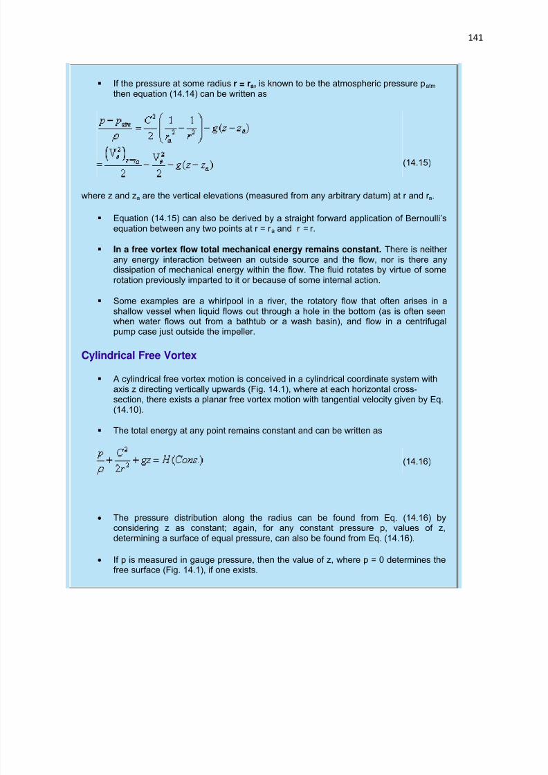
7/29/2019 FLUID MECHANICS LECTURE NOTES
http://slidepdf.com/reader/full/fluid-mechanics-lecture-notes 141/297
141
If the pressure at some radius r = ra, is known to be the atmospheric pressure patm then equation (14.14) can be written as
(14.15)
where z and za are the vertical elevations (measured from any arbitrary datum) at r and r a.
Equation (14.15) can also be derived by a straight forward application of Bernoulli’sequation between any two points at r = r a and r = r.
In a free vortex flow total mechanical energy remains constant. There is neither any energy interaction between an outside source and the flow, nor is there any
dissipation of mechanical energy within the flow. The fluid rotates by virtue of somerotation previously imparted to it or because of some internal action.
Some examples are a whirlpool in a river, the rotatory flow that often arises in ashallow vessel when liquid flows out through a hole in the bottom (as is often seenwhen water flows out from a bathtub or a wash basin), and flow in a centrifugalpump case just outside the impeller.
Cylindrical Free Vortex
A cylindrical free vortex motion is conceived in a cylindrical coordinate system withaxis z directing vertically upwards (Fig. 14.1), where at each horizontal cross-section, there exists a planar free vortex motion with tangential velocity given by Eq.
(14.10).
The total energy at any point remains constant and can be written as
(14.16)
The pressure distribution along the radius can be found from Eq. (14.16) byconsidering z as constant; again, for any constant pressure p, values of z,determining a surface of equal pressure, can also be found from Eq. (14.16).
If p is measured in gauge pressure, then the value of z, where p = 0 determines thefree surface (Fig. 14.1), if one exists.
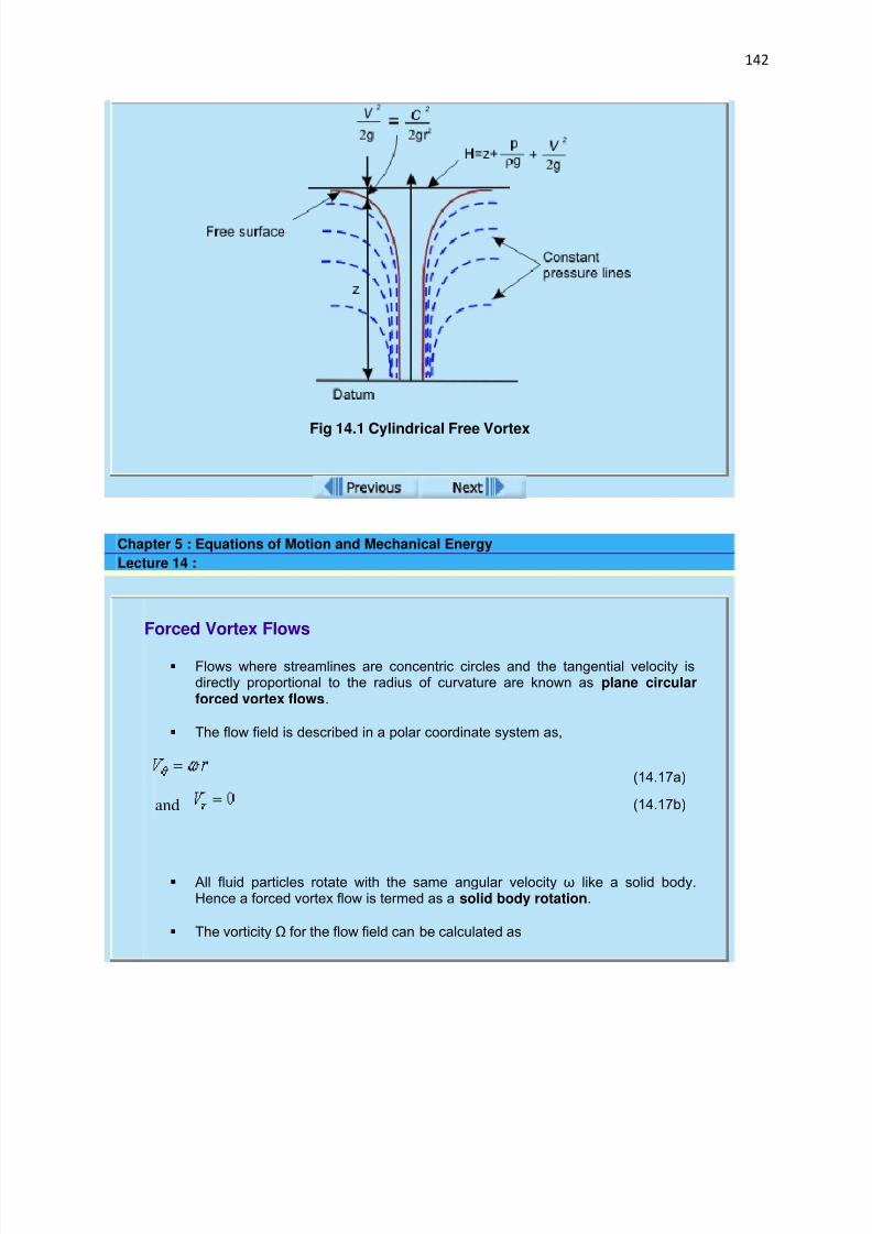
7/29/2019 FLUID MECHANICS LECTURE NOTES
http://slidepdf.com/reader/full/fluid-mechanics-lecture-notes 142/297

7/29/2019 FLUID MECHANICS LECTURE NOTES
http://slidepdf.com/reader/full/fluid-mechanics-lecture-notes 143/297
143
Therefore, a forced vortex motion is not irrotational; rather it is a rotational flowwith a constant vorticity 2ω. Equation (14.8) is used to determine thedistribution of mechanical energy across the radius as
Integrating the equation between the two radii on the same horizontal plane, wehave,
14.18)
Thus, we see from Eq. (14.18) that the total head (total energy per unit weight)increases with an increase in radius. The total mechanical energy at any pointis the sum of kinetic energy, flow work or pressure energy, and the potentialenergy.
Therefore the difference in total head between any two points in the samehorizontal plane can be written as,
Substituting this expression of H2-H1 in Eq. (14.18), we get
The same equation can also be obtained by integrating the equation of motionin a radial direction as

7/29/2019 FLUID MECHANICS LECTURE NOTES
http://slidepdf.com/reader/full/fluid-mechanics-lecture-notes 144/297
144
To maintain a forced vortex flow, mechanical energy has to be spent fromoutside and thus an external torque is always necessary to be appliedcontinuously.
Forced vortex can be generated by rotating a vessel containing a fluid so thatthe angular velocity is the same at all points.
Chapter 5 : Equations of Motion and Mechanical Energy
Lecture 14 :
7/29/2019 FLUID MECHANICS LECTURE NOTES
http://slidepdf.com/reader/full/fluid-mechanics-lecture-notes 145/297
145
Losses Due to Geometric Changes
In case of flow of a real fluid, the major source for the loss of its totalmechanical energy is the viscosity of fluid which causes friction between layersof fluid and between the solid surface and adjacent fluid layer.
Loss of Energy
It is the role of friction, as an agent, to convert a part of the mechanical energyinto intermolecular energy. This part of the mechanical energy converted into
the intermolecular energy is termed as the loss of energy.
When the path of the fluid is suddenly changed in course of its flow through aclosed duct due to any abrupt change in the geometry of the duct then apartfrom the losses due to friction between solid surface and fluid layer past it, theloss of mechanical energy is also incurred. In long ducts, these losses are verysmall compared to the frictional loss, and hence they are often termed as
minor losses.
But minor losses may, however, outweight the friction loss in short pipes or ducts. The source of these losses is usually confined to a very short length of the duct, but the turbulence produced may persist for a considerable distancedownstream.
Example of some minor Loss
Losses Due to Sudden Enlargement
Exit Loss
Losses Due to Sudden Contraction
Entry Loss
We'll discuss them individually in the next consequent slides
Chapter 5 : Equations of Motion and Mechanical Energy
Lecture 14 :
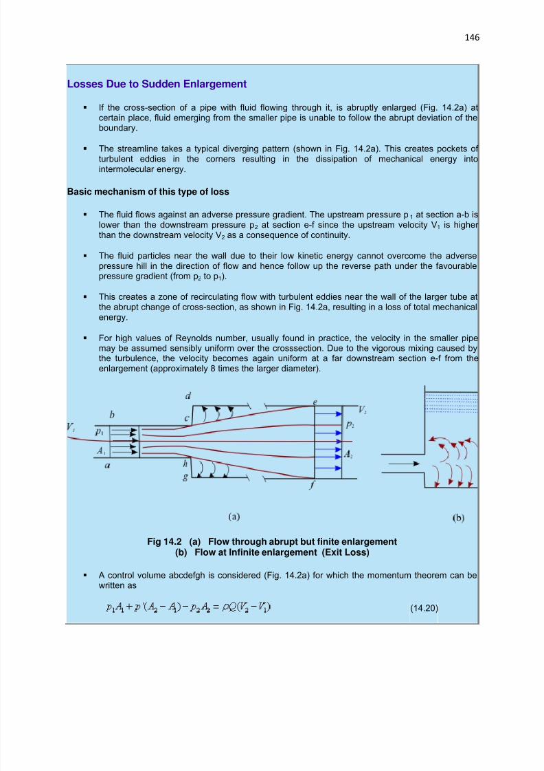
7/29/2019 FLUID MECHANICS LECTURE NOTES
http://slidepdf.com/reader/full/fluid-mechanics-lecture-notes 146/297
146
Losses Due to Sudden Enlargement
If the cross-section of a pipe with fluid flowing through it, is abruptly enlarged (Fig. 14.2a) atcertain place, fluid emerging from the smaller pipe is unable to follow the abrupt deviation of theboundary.
The streamline takes a typical diverging pattern (shown in Fig. 14.2a). This creates pockets of turbulent eddies in the corners resulting in the dissipation of mechanical energy intointermolecular energy.
Basic mechanism of this type of loss
The fluid flows against an adverse pressure gradient. The upstream pressure p 1 at section a-b islower than the downstream pressure p2 at section e-f since the upstream velocity V1 is higher than the downstream velocity V2 as a consequence of continuity.
The fluid particles near the wall due to their low kinetic energy cannot overcome the adverse
pressure hill in the direction of flow and hence follow up the reverse path under the favourablepressure gradient (from p2 to p1).
This creates a zone of recirculating flow with turbulent eddies near the wall of the larger tube atthe abrupt change of cross-section, as shown in Fig. 14.2a, resulting in a loss of total mechanicalenergy.
For high values of Reynolds number, usually found in practice, the velocity in the smaller pipemay be assumed sensibly uniform over the crosssection. Due to the vigorous mixing caused bythe turbulence, the velocity becomes again uniform at a far downstream section e-f from theenlargement (approximately 8 times the larger diameter).
Fig 14.2 (a) Flow through abrupt but finite enlargement(b) Flow at Infinite enlargement (Exit Loss)
A control volume abcdefgh is considered (Fig. 14.2a) for which the momentum theorem can bewritten as
(14.20)
7/29/2019 FLUID MECHANICS LECTURE NOTES
http://slidepdf.com/reader/full/fluid-mechanics-lecture-notes 147/297
147
where A1, A2 are the cross-sectional areas of the smaller and larger parts of the pipe respectively, Q isthe volumetric fllow rate and p’ is the mean pressure of the eddying fluid over the annular face, gd. It isknown from experimental evidence, the p’ = p1.
Hence the Eq. (14.20) becomes
(14.21)
From the equation of continuity
(14.22)
With the help of Eq. (14.22), Eq. (14.21) becomes
(14.23)
Applying Bernoulli's equation between sections ab and ef in consideration of the flow to be
incompressible and the axis of the pipe to be horizontal, we can write
(14.24)
where hL is the loss of head. Substituting (p2 −p1) from Eq. (14.23) into Eq. (14.24), we obtain
(14.25)

7/29/2019 FLUID MECHANICS LECTURE NOTES
http://slidepdf.com/reader/full/fluid-mechanics-lecture-notes 148/297
148
In view of the assumptions made, Eq.(14.25) is subjected to some inaccuracies, but experimentsshow that for coaxial pipes they are within only a few per cent of the actual values.
Back to original slide - "Losses due to geometric changes"
Exit Loss
If, in Eq.(14.25), , then the head loss at an abrupt enlargement tends to . Thephysical resemblance of this situation is the submerged outlet of a pipe discharging into a largereservoir as shown in Fig.14.2b.
Since the fluid velocities are arrested in the large reservoir, the entire kinetic energy at the outletof the pipe is dissipated into intermolecular energy of the reservoir through the creation of turbulent eddies.
In such circumstances, the loss is usually termed as the exit loss for the pipe and equals to thevelocity head at the discharge end of the pipe.
Back to original slide - "Losses due to geometric changes"
Chapter 5 : Equations of Motion and Mechanical Energy
Lecture 14 :
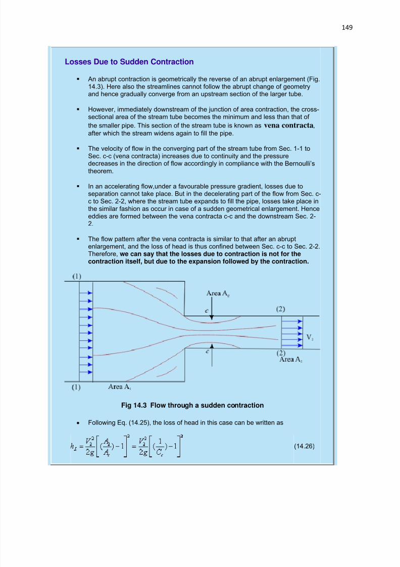
7/29/2019 FLUID MECHANICS LECTURE NOTES
http://slidepdf.com/reader/full/fluid-mechanics-lecture-notes 149/297
149
Losses Due to Sudden Contraction
An abrupt contraction is geometrically the reverse of an abrupt enlargement (Fig.14.3). Here also the streamlines cannot follow the abrupt change of geometryand hence gradually converge from an upstream section of the larger tube.
However, immediately downstream of the junction of area contraction, the cross-sectional area of the stream tube becomes the minimum and less than that of
the smaller pipe. This section of the stream tube is known as vena contracta,
after which the stream widens again to fill the pipe.
The velocity of flow in the converging part of the stream tube from Sec. 1-1 toSec. c-c (vena contracta) increases due to continuity and the pressuredecreases in the direction of flow accordingly in complianc e with the Bernoulli’stheorem.
In an accelerating flow,under a favourable pressure gradient, losses due toseparation cannot take place. But in the decelerating part of the flow from Sec. c-c to Sec. 2-2, where the stream tube expands to fill the pipe, losses take place inthe similar fashion as occur in case of a sudden geometrical enlargement. Henceeddies are formed between the vena contracta c-c and the downstream Sec. 2-2.
The flow pattern after the vena contracta is similar to that after an abruptenlargement, and the loss of head is thus confined between Sec. c-c to Sec. 2-2.Therefore, we can say that the losses due to contraction is not for thecontraction itself, but due to the expansion followed by the contraction.
Fig 14.3 Flow through a sudden contraction
Following Eq. (14.25), the loss of head in this case can be written as
(14.26)

7/29/2019 FLUID MECHANICS LECTURE NOTES
http://slidepdf.com/reader/full/fluid-mechanics-lecture-notes 150/297
150
where Ac represents the cross-sectional area of the vena contracta, and Cc is thecoefficient of contraction defined by
(14.27)
Equation (14.26) is usually expressed as
(14.28)
where,
(14.29)
Although the area A1 is not explicitly involved in the Eq. (14.26), the value of Cc depends on the ratio A2/A1. For coaxial circular pipes and at fairly highReynolds numbers. Table 14.1 gives representative values of the coefficient K.
Table 14.1
A2/A1 0 0.04 0.16 0.36 0.64 1.0
K 0.5 0.45 0.38 0.28 0.14 0
Back to original slide - "Losses due to geometric changes"
Entry Loss
As , the value of K in the Eq. (14.29) tends to 0.5 as shown in Table14.1. This limiting situation corresponds to the flow from a large reservoir into asharp edged pipe, provided the end of the pipe does not protrude into the
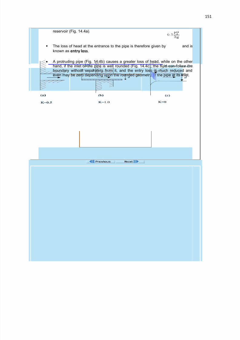
7/29/2019 FLUID MECHANICS LECTURE NOTES
http://slidepdf.com/reader/full/fluid-mechanics-lecture-notes 151/297
151
reservoir (Fig. 14.4a).
The loss of head at the entrance to the pipe is therefore given by and is
known as entry loss.
A protruding pipe (Fig. 14.4b) causes a greater loss of head, while on the other hand, if the inlet of the pipe is well rounded (Fig. 14.4c), the fluid can follow theboundary without separating from it, and the entry loss is much reduced andeven may be zero depending upon the rounded geometry of the pipe at its inlet.
Fig 14.4 Flow from a reservoir to a sharp edges pipe
Back to original slide - "Losses due to geometric changes"
End of Lecture 14!
To start next lecture click next
button or select from left-hand-
side.
7/29/2019 FLUID MECHANICS LECTURE NOTES
http://slidepdf.com/reader/full/fluid-mechanics-lecture-notes 152/297
152
Chapter 5 : Applications of Equations of Motion and Mechanical Energy
Lecture 15 :
Measurement Of Flow Rate Through Pipe
Flow rate through a pipe is usually measured by providing a coaxial area contraction within thepipe and by recording the pressure drop across the contraction. Therefore the determination of the flow rate from the measurement of pressure drop depends on the straight forward applicationof Bernoulli’s equation.
Three different flow meters operate on this principle.
Venturimeter Orificemeter Flow nozzle.
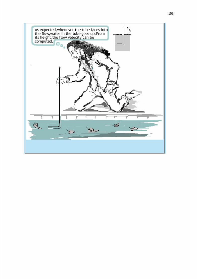
7/29/2019 FLUID MECHANICS LECTURE NOTES
http://slidepdf.com/reader/full/fluid-mechanics-lecture-notes 153/297
153
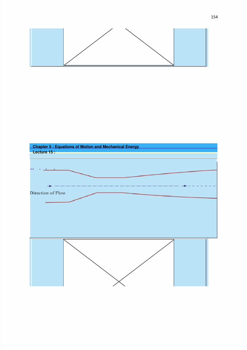
7/29/2019 FLUID MECHANICS LECTURE NOTES
http://slidepdf.com/reader/full/fluid-mechanics-lecture-notes 154/297
154
Chapter 5 : Equations of Motion and Mechanical Energy
Lecture 15 :
Venturimeter
Construction: A venturimeter is essentially a short pipe (Fig. 15.1) consisting of two conical parts with ashort portion of uniform cross-section in between. This short portion has the minimum area and is knownas the throat. The two conical portions have the same base diameter, but one is having a shorter lengthwith a larger cone angle while the other is having a larger length with a smaller cone angle.
Fig 15.1 A Venturimeter
Working:
The venturimeter is always used in a way that the upstream part of the flow takes place through
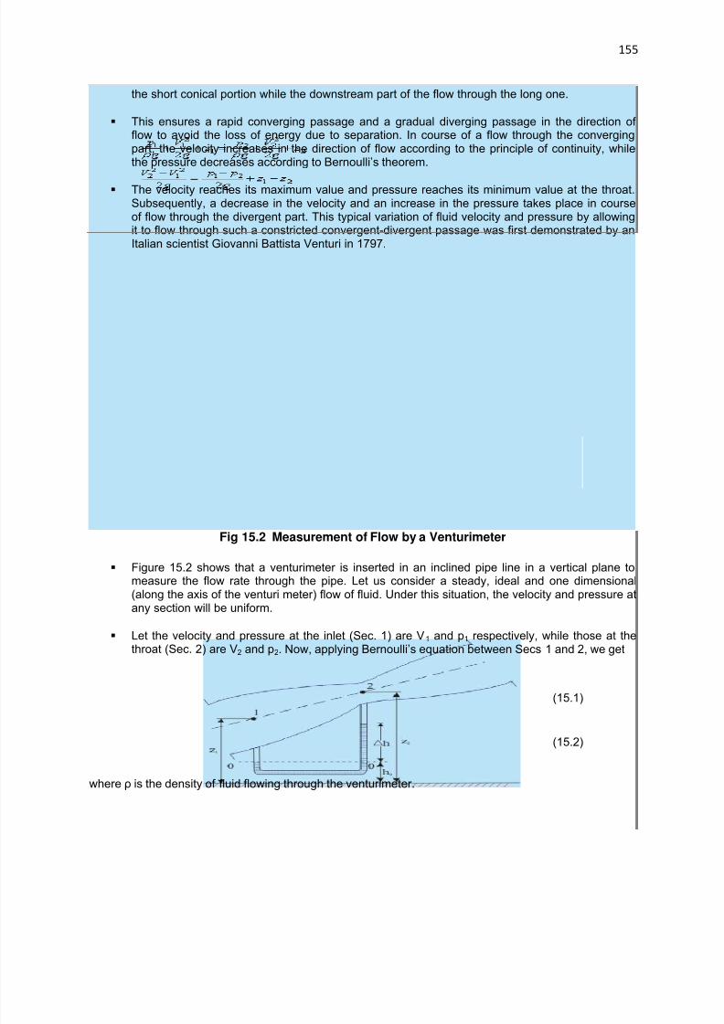
7/29/2019 FLUID MECHANICS LECTURE NOTES
http://slidepdf.com/reader/full/fluid-mechanics-lecture-notes 155/297
155
the short conical portion while the downstream part of the flow through the long one.
This ensures a rapid converging passage and a gradual diverging passage in the direction of flow to avoid the loss of energy due to separation. In course of a flow through the convergingpart, the velocity increases in the direction of flow according to the principle of continuity, whilethe pressure decreases according to Bernoulli’s theorem.
The velocity reaches its maximum value and pressure reaches its minimum value at the throat.Subsequently, a decrease in the velocity and an increase in the pressure takes place in courseof flow through the divergent part. This typical variation of fluid velocity and pressure by allowingit to flow through such a constricted convergent-divergent passage was first demonstrated by anItalian scientist Giovanni Battista Venturi in 1797.
Fig 15.2 Measurement of Flow by a Venturimeter
Figure 15.2 shows that a venturimeter is inserted in an inclined pipe line in a vertical plane tomeasure the flow rate through the pipe. Let us consider a steady, ideal and one dimensional(along the axis of the venturi meter) flow of fluid. Under this situation, the velocity and pressure atany section will be uniform.
Let the velocity and pressure at the inlet (Sec. 1) are V 1 and p1 respectively, while those at thethroat (Sec. 2) are V2 and p2. Now, applying Bernoulli’s equation between Secs 1 and 2, we get
(15.1)
(15.2)
where ρ is the density of fluid flowing through the venturimeter.
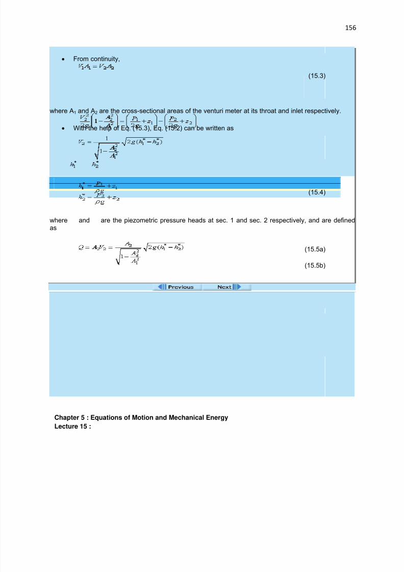
7/29/2019 FLUID MECHANICS LECTURE NOTES
http://slidepdf.com/reader/full/fluid-mechanics-lecture-notes 156/297
156
From continuity,
(15.3)
where A1 and A2 are the cross-sectional areas of the venturi meter at its throat and inlet respectively.
With the help of Eq. (15.3), Eq. (15.2) can be written as
(15.4)
where and are the piezometric pressure heads at sec. 1 and sec. 2 respectively, and are definedas
(15.5a)
(15.5b)
Hence, the volume flow rate through the pipe is given by
(15.6)
(Venturimeter continued....),
Chapter 5 : Equations of Motion and Mechanical Energy
Lecture 15 :

7/29/2019 FLUID MECHANICS LECTURE NOTES
http://slidepdf.com/reader/full/fluid-mechanics-lecture-notes 157/297
157
...Venturimeter... contd from previous slide
If the pressure difference between Sections 1 and 2 is measured by amanometer as shown in Fig. 15.2, we can write
(15.7)
where ρm is the density of the manometric liquid.
Equation (15.7) shows that a manometer always registers a direct reading of
the difference in piezometric pressures. Now, substitution of from Eq.(15.7) in Eq. (15.6) gives
(15.8)
If the pipe along with the venturimeter is horizontal, then z1 = z2; and hence
becomes h1 − h2, where h1 and h2 are the static pressure heads
The manometric equation Eq. (15.7) then becomes
Therefore, it is interesting to note that the final expression of flow rate, given byEq. (15.8), in terms of manometer deflection ∆h, remains the same irrespectiveof whether the pipe-line along with the venturimeter connection is horizontal or not.

7/29/2019 FLUID MECHANICS LECTURE NOTES
http://slidepdf.com/reader/full/fluid-mechanics-lecture-notes 158/297
158
Measured values of ∆h, the difference in piezometric pressures between Secs Iand 2, for a real fluid will always be greater than that assumed in case of anideal fluid because of frictional losses in addition to the change in momentum.
Therefore, Eq. (15.8) always overestimates the actual flow rate. In order to takethis into account, a multiplying factor Cd, called the coefficient of discharge, is
incorporated in the Eq. (15.8) as
The coefficient of discharge Cd is always less than unity and is defined as
where, the theoretical discharge rate is predicted by the Eq. (15.8) with the measuredvalue of ∆h, and the actual rate of discharge is the discharge rate measured in practice.Value of Cd for a venturimeter usually lies between 0.95 to 0.98.
Chapter 5 : Applications of Equations of Motion and Mechanical Energy
Lecture 15 :

7/29/2019 FLUID MECHANICS LECTURE NOTES
http://slidepdf.com/reader/full/fluid-mechanics-lecture-notes 159/297
159
Orificemeter
Construction: An orificemeter provides a simpler and cheaper arrangement for themeasurement of fow through a pipe. An orificemeter is essentially a thin circular platewith a sharp edged concentric circular hole in it.
Working:
The orifice plate, being fixed at a section of the pipe, (Fig. 15.3) creates anobstruction to the flow by providing an opening in the form of an orifice to theflow passage.
Fig 15.3 Flow through an Orificemeter
The area A0 of the orifice is much smaller than the cross-sectional area of thepipe. The flow from an upstream section, where it is uniform, adjusts itself insuch a way that it contracts until a section downstream the orifice plate isreached, where the vena contracta is formed, and then expands to fill thepassage of the pipe.
One of the pressure tapings is usually provided at a distance of one diameter upstream the orifice plate where the flow is almost uniform (Sec. 1-1) and theother at a distance of half a diameter downstream the orifice plate.
Considering the fluid to be ideal and the downstream pressure taping to be atthe vena contracta (Sec. c-c), we can write, by applying Bernoulli’s theorembetween Sec. 1-1 and Sec. c-c,
(15.10)
where and are the piezometric pressures at Sec.1-1 and c-c respectively.
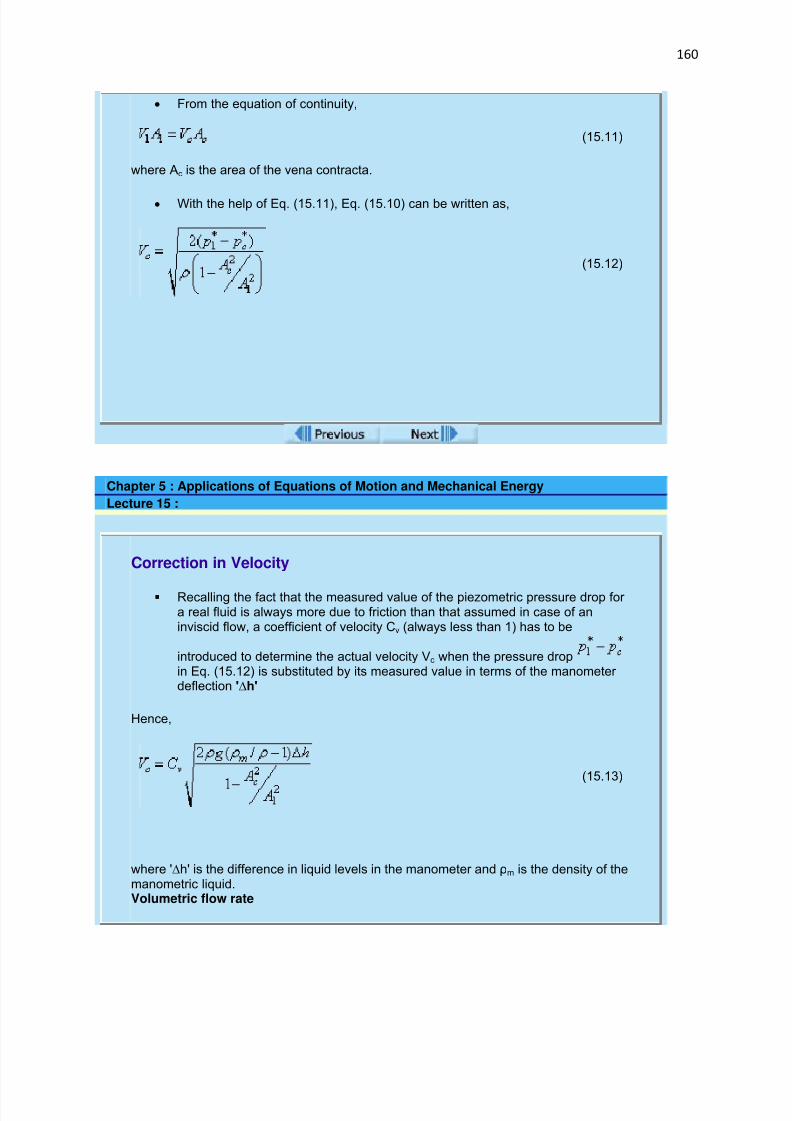
7/29/2019 FLUID MECHANICS LECTURE NOTES
http://slidepdf.com/reader/full/fluid-mechanics-lecture-notes 160/297
160
From the equation of continuity,
(15.11)
where Ac is the area of the vena contracta.
With the help of Eq. (15.11), Eq. (15.10) can be written as,
(15.12)
Chapter 5 : Applications of Equations of Motion and Mechanical Energy
Lecture 15 :
Correction in Velocity
Recalling the fact that the measured value of the piezometric pressure drop for a real fluid is always more due to friction than that assumed in case of aninviscid flow, a coefficient of velocity Cv (always less than 1) has to be
introduced to determine the actual velocity Vc when the pressure dropin Eq. (15.12) is substituted by its measured value in terms of the manometer deflection '∆h'
Hence,
(15.13)
where '∆h' is the difference in liquid levels in the manometer and ρm is the density of themanometric liquid.Volumetric flow rate

7/29/2019 FLUID MECHANICS LECTURE NOTES
http://slidepdf.com/reader/full/fluid-mechanics-lecture-notes 161/297
161
(15.14)
If a coefficient of contraction Cc is defined as, Cc = Ac /A0, where A0 is thearea of the orifice, then Eq.(15.14) can be written, with the help of Eq. (15.13),
(15.15)
The value of C depends upon the ratio of orifice to duct area, and the Reynolds number of flow.
The main job in measuring the flow rate with the help of an orificemeter, is tofind out accurately the value of C at the operating condition.
The downstream manometer connection should strictly be made to the sectionwhere the vena contracta occurs, but this is not feasible as the vena contractais somewhat variable in position and is difficult to realize.
In practice, various positions are used for the manometer connections and C isthereby affected. Determination of accurate values of C of an orificemeterat different operating conditions is known as calibration of the orificemeter.
Chapter 5 : Applications of Equations of Motion and Mechanical Energy
Lecture 15 :

7/29/2019 FLUID MECHANICS LECTURE NOTES
http://slidepdf.com/reader/full/fluid-mechanics-lecture-notes 162/297
162
Flow Nozzle
The flow nozzle as shown in Fig.15.4 is essentially a venturi meter with the divergent partomitted. Therefore the basic equations for calculation of flow rate are the same as thosefor a venturimeter.
The dissipation of energy downstream of the throat due to flow separation is greater thanthat for a venturimeter. But this disadvantage is often offset by the lower cost of thenozzle.
The downstream connection of the manometer may not necessarily be at the throat of thenozzle or at a point sufficiently far from the nozzle.
The deviations are taken care of in the values of C d, The coefficient Cd depends on theshape of the nozzle, the ratio of pipe to nozzle diameter and the Reynolds numberof flow.
Fig 15.4 A Flow nozzle
A comparative picture of the typical values of C d, accuracy, and the cost of three flowmeters (venturimeter, orificemeter and flow nozzle) is given below:
Type of Flowmeter Accuracy CostLoss of
Total Head
Typical Valuesof Cd
Venturimeter High High Low 0.95 to 0.98
Orificemeter Low Low High 0.60 to 0.65
Flow NozzleIntermediate betweena venturimeter and anorificemeter
0.70 to 0.80
End of Lecture 15!
To start next lecture click next buttonor select from left-hand-side.
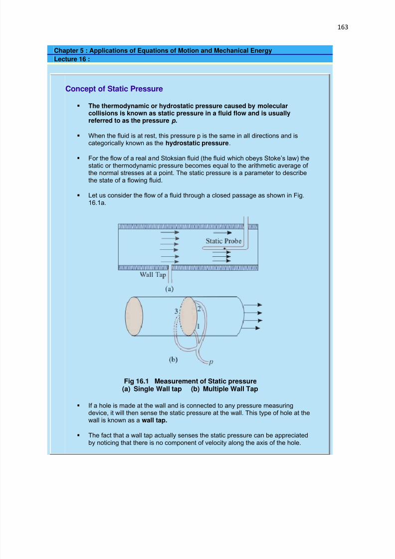
7/29/2019 FLUID MECHANICS LECTURE NOTES
http://slidepdf.com/reader/full/fluid-mechanics-lecture-notes 163/297
163
Chapter 5 : Applications of Equations of Motion and Mechanical Energy
Lecture 16 :
Concept of Static Pressure
The thermodynamic or hydrostatic pressure caused by molecularcollisions is known as static pressure in a fluid flow and is usuallyreferred to as the pressure p .
When the fluid is at rest, this pressure p is the same in all directions and iscategorically known as the hydrostatic pressure.
For the flow of a real and Stoksian fluid (the fluid which obeys Stoke’s law) thestatic or thermodynamic pressure becomes equal to the arithmetic average of the normal stresses at a point. The static pressure is a parameter to describethe state of a flowing fluid.
Let us consider the flow of a fluid through a closed passage as shown in Fig.16.1a.
Fig 16.1 Measurement of Static pressure
(a) Single Wall tap (b) Multiple Wall Tap
If a hole is made at the wall and is connected to any pressure measuringdevice, it will then sense the static pressure at the wall. This type of hole at thewall is known as a wall tap.
The fact that a wall tap actually senses the static pressure can be appreciatedby noticing that there is no component of velocity along the axis of the hole.

7/29/2019 FLUID MECHANICS LECTURE NOTES
http://slidepdf.com/reader/full/fluid-mechanics-lecture-notes 164/297
164
In most circumstances, for example, in case of parallel flows, the static pressureat a cross-section remains the same. The wall tap under this situation registersthe static pressure at that cross-section.
In practice, instead of a single wall tap, a number of taps along the periphery of the wall are made and are mutually connected by flexible tubes (Fig. 16.1b) in
order to register the static pressure more accurately.
Chapter 5 : Applications of Equations of Motion and Mechanical Energy
Lecture 16 :
Hydrostatic, Hydrodynamic, Static and Total Pressure
Let us consider a fluid flowing through a pipe of varying cross sectional area.Considering two points A and B as shown in Figure 16.1(c), such that A andB are at a height Z A and ZB respectively from the datum.
Figure 16.1 (c)
If we consider the fluid to be stationary, then, where the
subscript ‘hs’ represents the hydrostatic case.
So, p Ahs - pBhs = ρg( ZB –Z A)
(16.1)
where p Ahs is the hydrostatic pressure at A and pBhs is the hydrostatic pressure at B.
Thus, from above we can conclude that the Hydrostatic pressure at a pointin a fluid is the pressure acting at the point when the fluid is at rest or
7/29/2019 FLUID MECHANICS LECTURE NOTES
http://slidepdf.com/reader/full/fluid-mechanics-lecture-notes 165/297
165
pressure at the point due to weight of the fluid above it.
Now if we consider the fluid to be moving, the pressure at a point can bewritten as a sum of two components, Hydrodynamic and Hydrostatic.
p A = p Ahs + p Ahd (16.2)
here p Ahs is the hydrostatic pressure at A and p Ahd is the hydrodynamic pressure at.
Using equation (16.2) in Bernoulli's equation between points A and B.
(16.3)
From equation (16.1), the terms within the square bracket cancel each other.
Hence,
(16.4)
(16.5)
Equations (16.4) and (16.5) convey the following. The pressure at alocation has both hydrostatic and hydrodynamic components. Thedifference in kinetic energy arises due to hydrodynamic componentsonly.
In a frictionless flow, the sum of flow work due to hydrodynamic pressureand the kinetic energy is conserved. Such conservation shall apply to theentire flow field if the flow is irrotational.
The hydrodynamic component is often called static pressure and thevelocity term, dynamic pressure. The sum of two, p0 is known as totalpressure. This is conserved in isentropic, irrotational flow.

7/29/2019 FLUID MECHANICS LECTURE NOTES
http://slidepdf.com/reader/full/fluid-mechanics-lecture-notes 166/297
166
Chapter 5 : Applications of Equations of Motion and Mechanical Energy
Lecture 16 :
Stagnation Pressure
The stagnation pressure at a point in a fluid flow is the pressure which couldresult if the fluid were brought to rest isentropically.
The word isentropically implies the sense that the entire kinetic energy of afluid particle is utilized to increase its pressure only. This is possible only in areversible adiabatic process known as isentropic process.
Fig 16.2 Measurement of Stagnation Pressure
Let us consider the flow of fluid through a closed passage (Fig. 16.2). AtSec. l-l let the velocity and static pressure of the fluid be uniform. Consider apoint A on that section just in front of which a right angled tube with one endfacing the flow and the other end closed is placed.
When equilibrium is attained, the fluid in the tube will be at rest, and the
pressure at any point in the tube including the point B will be more than thatat A where the flow velocity exists.
By the application of Bernoulli’s equation between the points B and A, inconsideration of the flow to be inviscid and incompressible, we have,
(16.6)

7/29/2019 FLUID MECHANICS LECTURE NOTES
http://slidepdf.com/reader/full/fluid-mechanics-lecture-notes 167/297
167
here p and V are the pressure and velocity respectively at the point A at Sec. I-I,and p0 is the pressure at B which, according to the definition, refers to the stagnationpressure at point A.
It is found from Eq. (16.6) that the stagnation pressure p0 consists of twoterms, the static pressure, p and the term ρV
2/2 which is known as
dynamic pressure. Therefore Eq. (16.6) can be written for a better understanding as
(16.7)
Therefore, it appears from Eq.(16.7), that from a measurement of both staticand stagnation pressure in a flowing fluid, the velocity of flow can bedetermined.
But it is difficult to measure the stagnation pressure in practice for a real fluid
due to friction. The pressure in the stagnation tube indicated by anypressure measuring device (Fig. 16.2) will always be less than p 0, since apart of the kinetic energy will be converted into intermolecular energy due tofluid friction). This is taken care of by an empirical factor C in determiningthe velocity from Eq. (16.7) as
(16.8)
Chapter 5 : Applications of Equations of Motion and Mechanical Energy
Lecture 16 :

7/29/2019 FLUID MECHANICS LECTURE NOTES
http://slidepdf.com/reader/full/fluid-mechanics-lecture-notes 168/297

7/29/2019 FLUID MECHANICS LECTURE NOTES
http://slidepdf.com/reader/full/fluid-mechanics-lecture-notes 169/297
169
determine the velocity. But for a fluid flowing through a closed duct, the Pitot tubemeasures only the stagnation pressure and so the static pressure must bemeasured separately.
Measurement of static pressure in this case is made at the boundary of the wall(Fig. 16.3b). The axis of the tube measuring the static pressure must be
perpendicular to the boundary and free from burrs, so that the boundary is smoothand hence the streamlines adjacent to it are not curved. This is done to sense thestatic pressure only without any part of the dynamic pressure.
A Pitot tube is also inserted as shown (Fig. 16.3b) to sense the stagnation pressure.The ends of the Pitot tube, measuring the stagnation pressure, and the piezometrictube, measuring the static pressure, may be connected to a suitable differentialmanometer for the determination of flow velocity and hence the flow rate.
Pitot Static Tube
The tubes recording static pressure and the stagnation pressure (Fig. 16.3b) areusually combined into one instrument known as Pitot static tube (Fig. 16.4).
Fig 16.4 Pitot Static Tube
The tube for sensing the static pressure is known as static tube which surrounds thepitot tube that measures the stagnation pressure.
Two or more holes are drilled radially through the outer wall of the static tube intoannular space. The position of these static holes is important. Downstream of the
nose N, the flow is accelerated somewhat with consequent reduction in staticpressure. But in front of the supporting stem, there is a reduction in velocity andincrease in pressure.
The static holes should therefore be at the position where the two opposing effectsare counterbalanced and the reading corresponds to the undisturbed staticpressure. Finally the flow velocity is given by
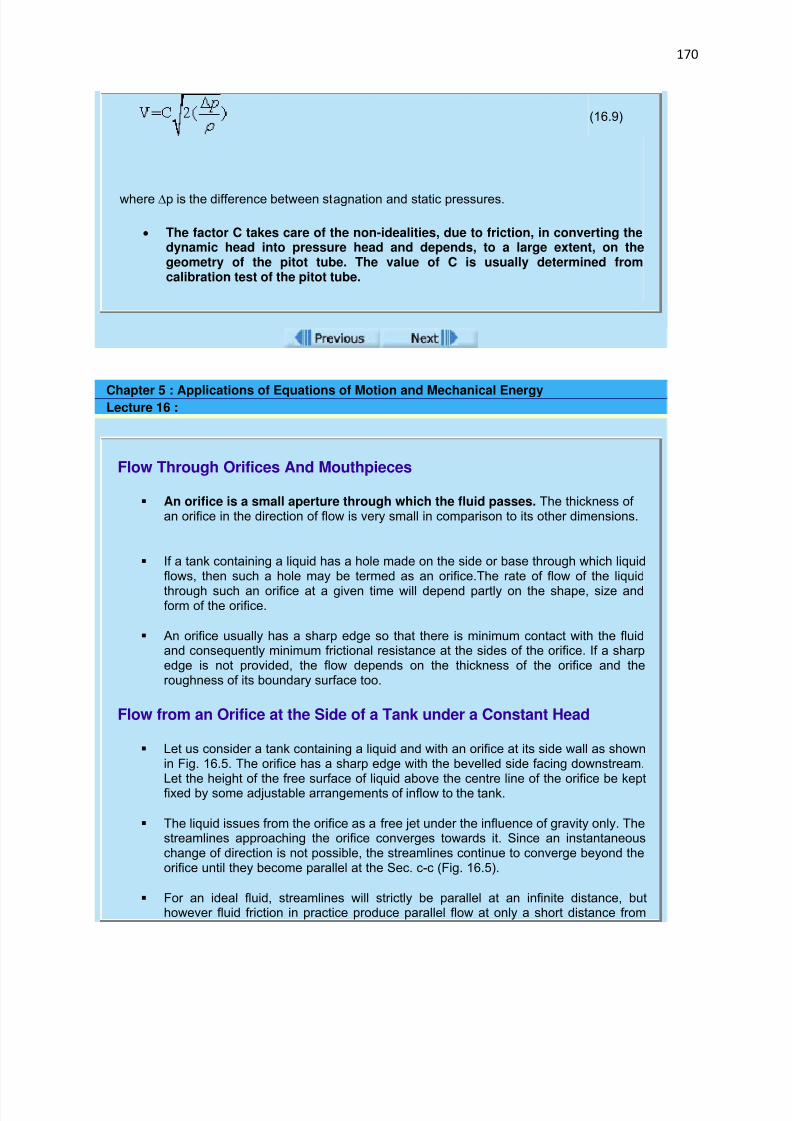
7/29/2019 FLUID MECHANICS LECTURE NOTES
http://slidepdf.com/reader/full/fluid-mechanics-lecture-notes 170/297
170
(16.9)
where ∆p is the difference between stagnation and static pressures.
The factor C takes care of the non-idealities, due to friction, in converting thedynamic head into pressure head and depends, to a large extent, on thegeometry of the pitot tube. The value of C is usually determined fromcalibration test of the pitot tube.
Chapter 5 : Applications of Equations of Motion and Mechanical EnergyLecture 16 :
Flow Through Orifices And Mouthpieces
An orifice is a small aperture through which the fluid passes. The thickness of an orifice in the direction of flow is very small in comparison to its other dimensions.
If a tank containing a liquid has a hole made on the side or base through which liquidflows, then such a hole may be termed as an orifice.The rate of flow of the liquid
through such an orifice at a given time will depend partly on the shape, size andform of the orifice.
An orifice usually has a sharp edge so that there is minimum contact with the fluidand consequently minimum frictional resistance at the sides of the orifice. If a sharpedge is not provided, the flow depends on the thickness of the orifice and theroughness of its boundary surface too.
Flow from an Orifice at the Side of a Tank under a Constant Head
Let us consider a tank containing a liquid and with an orifice at its side wall as shownin Fig. 16.5. The orifice has a sharp edge with the bevelled side facing downstream.Let the height of the free surface of liquid above the centre line of the orifice be keptfixed by some adjustable arrangements of inflow to the tank.
The liquid issues from the orifice as a free jet under the influence of gravity only. Thestreamlines approaching the orifice converges towards it. Since an instantaneouschange of direction is not possible, the streamlines continue to converge beyond theorifice until they become parallel at the Sec. c-c (Fig. 16.5).
For an ideal fluid, streamlines will strictly be parallel at an infinite distance, buthowever fluid friction in practice produce parallel flow at only a short distance from

7/29/2019 FLUID MECHANICS LECTURE NOTES
http://slidepdf.com/reader/full/fluid-mechanics-lecture-notes 171/297
171
the orifice. The area of the jet at the Sec. c-c is lower than the area of the orifice.The Sec. c-c is known as the vena contracta.
Fig 16.5 Flow from a Sharp edged Orifice
The contraction of the jet can be attributed to the action of a lateral force onthe jet due to a change in the direction of flow velocity when the fluid
approaches the orifice. Since the streamlines become parallel at vena contracta,the pressure at this section is assumed to be uniform.
If the pressure difference due to surface tension is neglected, the pressure in the jetat vena contracta becomes equal to that of the ambience surrounding the jet.
Considering the flow to be steady and frictional effects to be negligible, we can writeby the application of Bernoulli’s equation between two points 1 and 2 on a particular stream-line with point 2 being at vena contracta (Fig 16.5).
(16.10)
The horizontal plane through the centre of the orifice has been taken as datum levelfor determining the potential head.
If the area of the tank is large enough as compared to that of the orifice, the velocityat point 1 becomes negligibly small and pressure p1 equals to the hydrostaticpressure p1 equals to the hydrostatic pressure at that point as p 1=patm +ρg(h-z1).
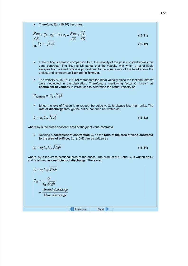
7/29/2019 FLUID MECHANICS LECTURE NOTES
http://slidepdf.com/reader/full/fluid-mechanics-lecture-notes 172/297
172
Therefore, Eq. (16.10) becomes
(16.11)
or, (16.12)
If the orifice is small in comparison to h, the velocity of the jet is constant across thevena contracta. The Eq. (16.12) states that the velocity with which a jet of liquidescapes from a small orifice is proportional to the square root of the head above theorifice, and is known as Torricelli’s formula.
The velocity V2 in Eq. (16.12) represents the ideal velocity since the frictional effectswere neglected in the derivation. Therefore, a multiplying factor Cv known ascoefficient of velocity is introduced to determine the actual velocity as
Since the role of friction is to reduce the velocity, C v is always less than unity. The rate of discharge through the orifice can then be written as,
(16.13)
where ac is the cross-sectional area of the jet at vena contracta.
Defining a coefficient of contraction Cc as the ratio of the area of vena contracta
to the area of orifiice, Eq. (16.8) can be written as
(16.14)
where, a0 is the cross-sectional area of the orifice. The product of Cc and Cv is written as Cd and is termed as coefficient of discharge. Therefore,
7/29/2019 FLUID MECHANICS LECTURE NOTES
http://slidepdf.com/reader/full/fluid-mechanics-lecture-notes 173/297
173
Module 3 :
Chapter 6 : Principles of Physical Similarity and Dimensional Analysis
Objectives
Lecture 17
Principles of Physical Similarity
Lecture 18
Magnitude of Different Forces acting on a Fluid Element
Dynamic Similarity of Flows with
Lecture 19
The Application of Dynamic Similarity - Dimension of Physical Quantity
Buckingham's Pi-Theorem
Rayleigh's Indical Method
Exercise Problem

7/29/2019 FLUID MECHANICS LECTURE NOTES
http://slidepdf.com/reader/full/fluid-mechanics-lecture-notes 174/297
174
Chapter 6 : Principles of Physical Similarity and Dimensional Analysis
Lecture 17 :
Concept and Types of Physical Similarity
The primary and fundamental requirement for the physical similarity between two problemsis that the physics of the problems must be the same.
For an example, two flows: one governed by viscous and pressure forces while the other bygravity force cannot be made physically similar. Therefore, the laws of similarity have to besought between problems described by the same physics.
Definition of physical similarity as a general proposition.
Two systems, described by the same physics, operating under different sets of conditionsare said to be physically similar in respect of certain specified physical quantities; when theratio of corresponding magnitudes of these quantities between the two systems is the sameeverywhere.
In the field of mechanics, there are three types of similarities which constitute the complete similaritybetween problems of same kind.
Geometric Similarity : If the specified physical quantities are geometrical dimensions, the similarity iscalled Geometric Similarty,
Kinematic Similarity : If the quantities are related to motions, the similarity is called Kinematic
Similarity
Dynamic Similarity : If the quantities refer to forces, then the similarity is termed as Dynamic
Similarity.
Chapter 6 : Principles of Physical Similarity and Dimensional Analysis
Lecture 17 :
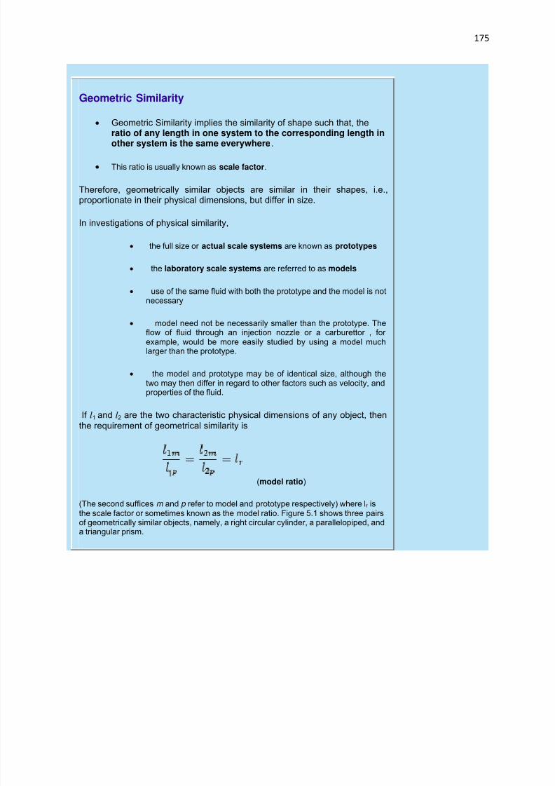
7/29/2019 FLUID MECHANICS LECTURE NOTES
http://slidepdf.com/reader/full/fluid-mechanics-lecture-notes 175/297
175
Geometric Similarity
Geometric Similarity implies the similarity of shape such that, the
ratio of any length in one system to the corresponding length inother system is the same everywhere.
This ratio is usually known as scale factor.
Therefore, geometrically similar objects are similar in their shapes, i.e.,proportionate in their physical dimensions, but differ in size.
In investigations of physical similarity,
the full size or actual scale systems are known as prototypes
the laboratory scale systems are referred to as models
use of the same fluid with both the prototype and the model is notnecessary
model need not be necessarily smaller than the prototype. Theflow of fluid through an injection nozzle or a carburettor , for example, would be more easily studied by using a model muchlarger than the prototype.
the model and prototype may be of identical size, although thetwo may then differ in regard to other factors such as velocity, andproperties of the fluid.
If l1 and l2 are the two characteristic physical dimensions of any object, thenthe requirement of geometrical similarity is
(model ratio)
(The second suffices m and p refer to model and prototype respectively) where lr isthe scale factor or sometimes known as the model ratio. Figure 5.1 shows three pairsof geometrically similar objects, namely, a right circular cylinder, a parallelopiped, anda triangular prism.

7/29/2019 FLUID MECHANICS LECTURE NOTES
http://slidepdf.com/reader/full/fluid-mechanics-lecture-notes 176/297
176
Fig 17.1 Geometrically Similar Objects
In all the above cases model ratio is 1/2
Geometric similarity is perhaps the most obvious requirement in a modelsystem designed to correspond to a given prototype system.
A perfect geometric similarity is not always easy to attain. Problems in achievingperfect geometric similarity are:
For a small model, the surface roughness might not be reduced accordingto the scale factor (unless the model surfaces can be made very muchsmoother than those of the prototype). If for any reason the scale factor isnot the same throughout, a distorted model results.
Sometimes it may so happen that to have a perfect geometric similaritywithin the available laboratory space, physics of the problem changes. For example, in case of large prototypes, such as rivers, the size of the model islimited by the available floor space of the laboratory; but if a very low scalefactor is used in reducing both the horizontal and vertical lengths, this mayresult in a stream so shallow that surface tension has a considerable effectand, moreover, the flow may be laminar instead of turbulent. In thissituation, a distorted model may be unavoidable (a lower scale factor ”for horizontal lengths while a relatively higher scale factor for vertical lengths.
7/29/2019 FLUID MECHANICS LECTURE NOTES
http://slidepdf.com/reader/full/fluid-mechanics-lecture-notes 177/297
177
The extent to which perfect geometric similarity should be sought thereforedepends on the problem being investigated, and the accuracy required fromthe solution.
Chapter 6 :
Principles ofPhysical Similarityand DimensionalAnalysis
Lecture 17 :
Kinematic Similarity
Kinematic similarity refers to similarity of motion.
Since motions are described by distance and time, it implies similarity of lengths (i.e.,
geometrical similarity) and, in addition, similarity of time intervals.
If the corresponding lengths in the two systems are in a fixed ratio, the velocities of correspondingparticles must be in a fixed ratio of magnitude of corresponding time intervals.
If the ratio of corresponding lengths, known as the scale factor, is lr and the ratio ofcorresponding time intervals is tr, then the magnitudes of corresponding velocities arein the ratio lr/tr and the magnitudes of corresponding accelerations are in the ratio lr/t
2 r.
A well-known example of kinematic similarity is found in a planetarium. Here the galaxiesof stars and planets in space are reproduced in accordance with a certain length scale andin simulating the motions of the planets, a fixed ratio of time intervals (and hence velocitiesand accelerations) is used.
When fluid motions are kinematically similar, the patterns formed by streamlines aregeometrically similar at corresponding times.
Since the impermeable boundaries also represent streamlines, kinematically similarflows are possible only past geometrically similar boundaries.
Therefore, geometric similarity is a necessary condition for the kinematic similarity to be achieved, but not the sufficient one.
For example, geometrically similar boundaries may ensure geometrically similar streamlines in thenear vicinity of the boundary but not at a distance from the boundary.
Chapter 6 : Principles of Physical Similarity and Dimensional Analysis
Lecture 17 :

7/29/2019 FLUID MECHANICS LECTURE NOTES
http://slidepdf.com/reader/full/fluid-mechanics-lecture-notes 178/297
178
Dynamic Similarity
Dynamic similarity is the similarity of forces .
In dynamically similar systems, the magnitudes of forces atcorrespondingly similar points in each system are in a fixed ratio.
In a system involving flow of fluid, different forces due to different causesmay act on a fluid element. These forces are as follows:
Viscous Force (due to viscosity)
Pressure Force ( due to different
in pressure)
Gravity Force (due to
gravitational attraction)Capillary Force (due to surface
tension)
Compressibility Force ( due to
elasticity)
According to Newton 's law, the resultant FR of all these forces, will causethe acceleration of a fluid element. Hence
(17.1)
Moreover, the inertia force is defined as equal and opposite to the
resultant accelerating force
= -
Therefore Eq. 17.1 can be expressed as
For dynamic similarity, the magnitude ratios of these forces have to be
same for both the prototype and the model. The inertia force isusually taken as the common one to describe the ratios as (or puttingin other form we equate the the non dimensionalised forces in the twosystems)
7/29/2019 FLUID MECHANICS LECTURE NOTES
http://slidepdf.com/reader/full/fluid-mechanics-lecture-notes 179/297
179
End of Lecture 17!
To start next lecture click next buttonor select from left-hand-side.
Chapter 6 :Principles ofPhysical Similarityand DimensionalAnalysis
Lecture 18 :
Magnitudes of Different Forces
A fluid motion, under all such forces is characterised by
1. Hydrodynamic parameters like pressure, velocity and acceleration due to gravity,
2. Rheological and other physical properties of the fluid involved, and3. Geometrical dimensions of the system.
It is important to express the magnitudes of different forces in terms of these parameters, toknow the extent of their influences on the different forces acting on a flluid element in thecourse of its flow.
Inertia Force
The inertia force acting on a fluid element is equal in magnitude to the mass of theelement multiplied by its acceleration.
The mass of a fluid element is proportional to ρl 3 where, ρ is the density of fluid and l
is the characteristic geometrical dimension of the system.
The acceleration of a fluid element in any direction is the rate at which its velocity inthat direction changes with time and is therefore proportional in magnitude to some
characteristic velocity V divided by some specified interval of time t. The time interval
t is proportional to the characteristic length l divided by the characteristic velocity V ,
so that the acceleration becomes proportional to V 2
/l.
The magnitude of inertia force is thus proportional to
This can be written as,
7/29/2019 FLUID MECHANICS LECTURE NOTES
http://slidepdf.com/reader/full/fluid-mechanics-lecture-notes 180/297
180
(18.1a)
Viscous Force
The viscous force arises from shear stress in a flow of fluid.
Therefore, we can write
Magnitude of viscous force = shear stress X surface area over which the shear stressacts
Again, shear stress = µ (viscosity) X rate of shear strain
where, rate of shear strain velocity gradient and surface area
Hence
(18.1b)
Pressure Force
The pressure force arises due to the difference of pressure in a flow field.
Hence it can be written as
(18.1c)
(where, p is some characteristic pressure difference in the flow.)
Gravity Force
The gravity force on a fluid element is its weight. Hence,
(18.1d)
(where g is the acceleration due to gravity or weight per unit mass)
7/29/2019 FLUID MECHANICS LECTURE NOTES
http://slidepdf.com/reader/full/fluid-mechanics-lecture-notes 181/297
181
Capillary or Surface Tension Force
The capillary force arises due to the existence of an interface between two fluids.
The surface tension force acts tangential to a surface .
It is equal to the coefficient of surface tension σ multiplied by the length of a linear element on the surface perpendicular to which the force acts.
Therefore,
(18.1e)
Compressibility or Elastic Force
Elastic force arises due to the compressibility of the fluid in course of its flow.
For a given compression (a decrease in volume), the increase in pressure isproportional to the bulk modulus of elasticity E
This gives rise to a force known as the elastic force.
Hence, for a given compression
(18.1f)
The flow of a fluid in practice does not involve all the forces simultaneously.
Therefore, the pertinent dimensionless parameters for dynamic similarity are derived from theratios of significant forces causing the flow.
Chapter 6 : Principles of Physical Similarity and Dimensional Analysis
Lecture 18 :

7/29/2019 FLUID MECHANICS LECTURE NOTES
http://slidepdf.com/reader/full/fluid-mechanics-lecture-notes 182/297
182
Dynamic Similarity of Flows governed by Viscous, Pressure andInertia Forces
The criterion of dynamic similarity for the flows controlled by viscous, pressureand inertia forces are derived from the ratios of the representative magnitudes of these forces with the help of Eq. (18.1a) to (18.1c) as follows:
|
(18.2a)
(18.2b)
The term is known as Reynolds number, Re after the name of thescientist who first developed it and is thus proportional to the magnitude ratio of inertia force to viscous force .(Reynolds number plays a vital role in the analysis of fluid flow)
The term is known as Euler number, Eu after the name of the scientistwho first derived it. The dimensionless terms Re and Eu represent the critieria of dynamic similarity for the flows which are affected only by viscous, pressure andinertia forces. Such instances, for example, are
1. the full flow of fluid in a completely closed conduit,
2. flow of air past a low-speed aircraft and
3. the flow of water past a submarine deeply submerged to produce no waveson the surface.
Hence, for a complete dynamic similarity to exist between the prototype and themodel for this class of flows, the Reynolds number, Re and Euler number, Eu haveto be same for the two (prototype and model). Thus
(18.2c)
(18.2d)
where, the suffix p and suffix m refer to the parameters for prototype and modelrespectively.
In practice, the pressure drop is the dependent variable, and hence it is comparedfor the two systems with the help of Eq. (18.2d), while the equality of Reynoldsnumber (Eq. (18.2c)) along with the equalities of other parameters in relation to
7/29/2019 FLUID MECHANICS LECTURE NOTES
http://slidepdf.com/reader/full/fluid-mechanics-lecture-notes 183/297
183
kinematic and geometric similarities are maintained.
The characteristic geometrical dimension l and the reference velocity V inthe expression of the Reynolds number may be any geometricaldimension and any velocity which are significant in determining thepattern of flow.
For internal flows through a closed duct, the hydraulic diameter of the ductDh and the average flow velocity at a section are invariably used for l and Vrespectively.
The hydraulic diameter Dh is defined as Dh= 4A/P where A and P are thecross-sectional area and wetted perimeter respectively.
Chapter 6 :Principles ofPhysicalSimilarity andDimensionalAnalysis
Lecture 18 :
Dynamic Similarity of Flows with Gravity, Pressure and Inertia Forces
A flow of the type in which significant forces are gravity force, pressure force andinertia force, is found when a free surface is present.
Examples can be
1. the flow of a liquid in an open channel.
2. the wave motion caused by the passage of a ship through water.3. the flows over weirs and spillways.
The condition for dynamic similarity of such flows requires
the equality of the Euler number Eu (the magnitude ratio of pressure to inertiaforce),
and
the equality of the magnitude ratio of gravity to inertia force at correspondingpoints in the systems being compared.
Thus ,
(18.2e)
In practice, it is often convenient to use the square root of this ratio so to deal with

7/29/2019 FLUID MECHANICS LECTURE NOTES
http://slidepdf.com/reader/full/fluid-mechanics-lecture-notes 184/297
184
the first power of the velocity.
From a physical point of view, equality of implies equality of asregard to the concept of dynamic similarity.
The reciprocal of the term is known as Froude number ( after WilliamFroude who first suggested the use of this number in the study of naval architecture. )
Hence Froude number, .
Therefore, the primary requirement for dynamic similarity between the prototype andthe model involving flow of fluid with gravity as the significant force, is the equalityof Froude number, Fr, i.e.,
(18.2f)
Chapter 6 : Principles of Physical Similarity and Dimensional Analysis
Lecture 18 :
Dynamic Similarity of Flows with Surface Tension as the Dominant
Force
Surface tension forces are important in certain classes of practical problems such as ,
1. flows in which capillary waves appear
2. flows of small jets and thin sheets of liquid injected by a nozzle in air 3. flow of a thin sheet of liquid over a solid surface.
Here the significant parameter for dynamic similarity is the magnitude ratio of thesurface tension force to the inertia force.
This can be written as
The term is usually known as Weber number, Wb (after the German navalarchitect Moritz Weber who first suggested the use of this term as a relevant parameter.)

7/29/2019 FLUID MECHANICS LECTURE NOTES
http://slidepdf.com/reader/full/fluid-mechanics-lecture-notes 185/297
185
Thus for dynamically similar flows (Wb)m =(Wb)p
i.e.,
Chapter 6 : Principles of Physical Similarity and Dimensional Analysis
Lecture 18 :
Dynamic Similarity of Flows with Elastic Force
When the compressibility of fluid in the course of its flow becomes significant, the elasticforce along with the pressure and inertia forces has to be considered.
Therefore, the magnitude ratio of inertia to elastic force becomes a relevant parameter for dynamic similarity under this situation.
Thus we can write,
(18.2h)
The parameter is known as Cauchy number ,( after the Frenchmathematician A.L. Cauchy)
If we consider the flow to be isentropic , then it can be written
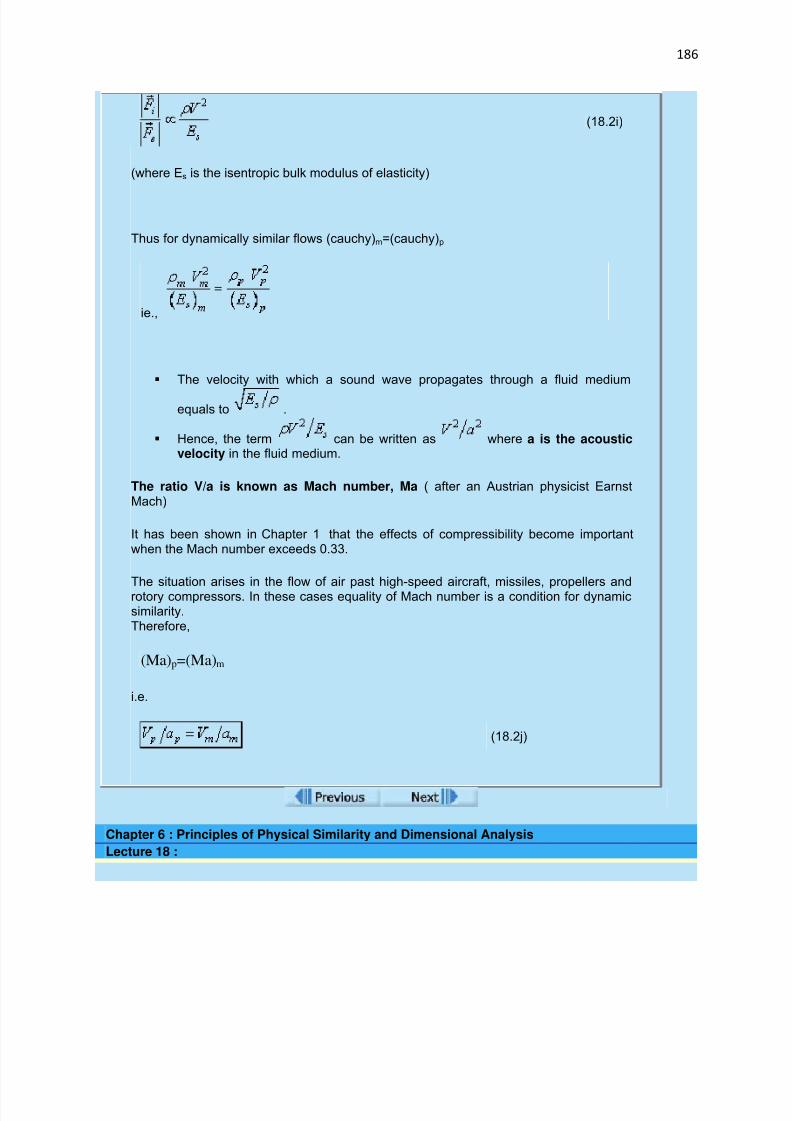
7/29/2019 FLUID MECHANICS LECTURE NOTES
http://slidepdf.com/reader/full/fluid-mechanics-lecture-notes 186/297
186
(18.2i)
(where Es is the isentropic bulk modulus of elasticity)
Thus for dynamically similar flows (cauchy)m=(cauchy)p
ie.,
The velocity with which a sound wave propagates through a fluid medium
equals to .
Hence, the term can be written as where a is the acousticvelocity in the fluid medium.
The ratio V/a is known as Mach number, Ma ( after an Austrian physicist EarnstMach)
It has been shown in Chapter 1 that the effects of compressibility become importantwhen the Mach number exceeds 0.33.
The situation arises in the flow of air past high-speed aircraft, missiles, propellers androtory compressors. In these cases equality of Mach number is a condition for dynamicsimilarity.Therefore,
(Ma)p=(Ma)m
i.e.
(18.2j)
Chapter 6 : Principles of Physical Similarity and Dimensional Analysis
Lecture 18 :
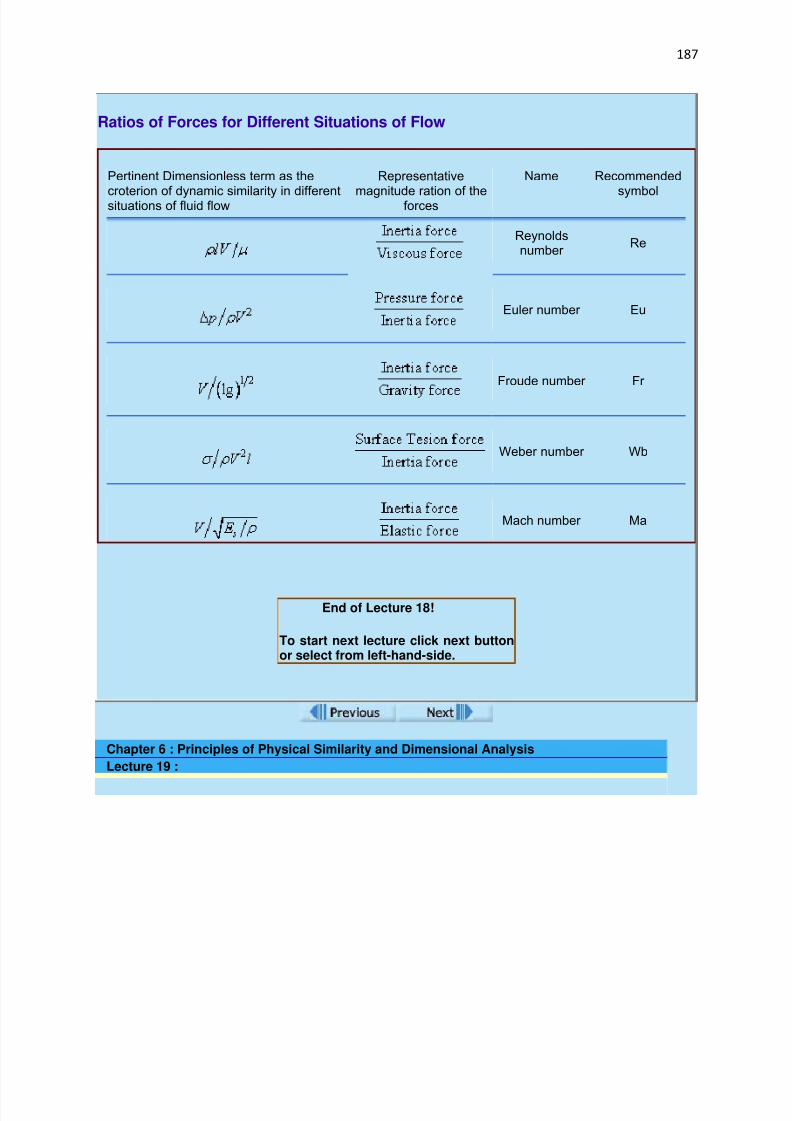
7/29/2019 FLUID MECHANICS LECTURE NOTES
http://slidepdf.com/reader/full/fluid-mechanics-lecture-notes 187/297
187
Ratios of Forces for Different Situations of Flow
Pertinent Dimensionless term as the
croterion of dynamic similarity in differentsituations of fluid flow
Representative
magnitude ration of theforces
Name Recommended
symbol
Reynoldsnumber
Re
Euler number Eu
Froude number Fr
Weber number Wb
Mach number Ma
End of Lecture 18!
To start next lecture click next buttonor select from left-hand-side.
Chapter 6 : Principles of Physical Similarity and Dimensional Analysis
Lecture 19 :

7/29/2019 FLUID MECHANICS LECTURE NOTES
http://slidepdf.com/reader/full/fluid-mechanics-lecture-notes 188/297
188
The Application of Dynamic Similarity - The Dimensional Analysis
The concept:
A physical problem may be characterised by a group of dimensionless similarityparameters or variables rather than by the original dimensional variables.
This gives a clue to the reduction in the number of parameters requiring separateconsideration in an experimental investigation.
For an example, if the Reynolds number Re = ρV Dh /µ is considered as theindependent variable, in case of a flow of fluid through a closed duct of hydraulicdiameter Dh, then a change in Re may be caused through a change in flow velocity Vonly. Thus a range of Re can be covered simply by the variation in V without varyingother independent dimensional variables ρ,Dh and µ.
In fact, the variation in the Reynolds number physically implies the variation in any of
the dimensional parameters defining it, though the change in Re, may be obtainedthrough the variation in anyone parameter, say the velocity V.
A number of such dimensionless parameters in relation to dynamic similarity areshown in Table 5.1. Sometimes it becomes diffcult to derive these parameters straightforward from an estimation of the representative order of magnitudes of the forcesinvolved. An alternative method of determining these dimensionless parameters bya mathematical technique is known as dimensional analysis .
The Technique:
The requirement of dimensional homogeneity imposes conditions on the quantities
involved in a physical problem, and these restrictions, placed in the form of an algebraicfunction by the requirement of dimensional homogeneity, play the central role indimensional analysis.
There are two existing approaches;
one due to Buckingham known as Buckingham's pi theorem
other due to Rayleigh known as Rayleigh's Indicial method
In our next slides we'll see few examples of the dimensions of physical quantities.
Chapter 6 : Principles of Physical Similarity and Dimensional Analysis
Lecture 19 :
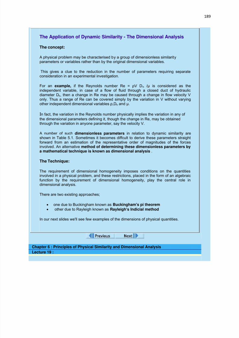
7/29/2019 FLUID MECHANICS LECTURE NOTES
http://slidepdf.com/reader/full/fluid-mechanics-lecture-notes 189/297
189
The Application of Dynamic Similarity - The Dimensional Analysis
The concept:
A physical problem may be characterised by a group of dimensionless similarityparameters or variables rather than by the original dimensional variables.
This gives a clue to the reduction in the number of parameters requiring separateconsideration in an experimental investigation.
For an example, if the Reynolds number Re = ρV Dh /µ is considered as theindependent variable, in case of a flow of fluid through a closed duct of hydraulicdiameter Dh, then a change in Re may be caused through a change in flow velocity Vonly. Thus a range of Re can be covered simply by the variation in V without varyingother independent dimensional variables ρ,Dh and µ.
In fact, the variation in the Reynolds number physically implies the variation in any of
the dimensional parameters defining it, though the change in Re, may be obtainedthrough the variation in anyone parameter, say the velocity V.
A number of such dimensionless parameters in relation to dynamic similarity areshown in Table 5.1. Sometimes it becomes diffcult to derive these parameters straightforward from an estimation of the representative order of magnitudes of the forcesinvolved. An alternative method of determining these dimensionless parameters bya mathematical technique is known as dimensional analysis .
The Technique:
The requirement of dimensional homogeneity imposes conditions on the quantities
involved in a physical problem, and these restrictions, placed in the form of an algebraicfunction by the requirement of dimensional homogeneity, play the central role indimensional analysis.
There are two existing approaches;
one due to Buckingham known as Buckingham's pi theorem
other due to Rayleigh known as Rayleigh's Indicial method
In our next slides we'll see few examples of the dimensions of physical quantities.
Chapter 6 : Principles of Physical Similarity and Dimensional Analysis
Lecture 19 :
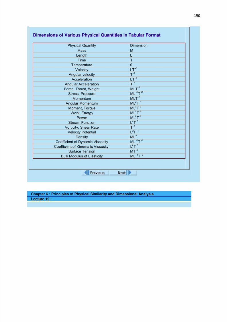
7/29/2019 FLUID MECHANICS LECTURE NOTES
http://slidepdf.com/reader/full/fluid-mechanics-lecture-notes 190/297
190
Dimensions of Various Physical Quantities in Tabular Format
Physical Quantity Dimension
Mass M
Length LTime T
Temperature θ
Velocity LT-1
Angular velocity T-
Acceleration LT-
Angular Acceleration T-
Force, Thrust, Weight MLT-
Stress, Pressure ML-
T-
Momentum MLT-1
Angular Momentum ML T-
Moment, Torque ML T-
Work, Energy ML T - Power ML T
-
Stream Function L T-
Vorticity, Shear Rate T-1
Velocity Potential L2T
-1
Density ML-
Coefficient of Dynamic Viscosity ML-
T-
Coefficient of Kinematic Viscosity L T-
Surface Tension MT-
Bulk Modulus of Elasticity ML-1
T-2
Chapter 6 : Principles of Physical Similarity and Dimensional Analysis
Lecture 19 :

7/29/2019 FLUID MECHANICS LECTURE NOTES
http://slidepdf.com/reader/full/fluid-mechanics-lecture-notes 191/297
191
Buckingham's Pi Theorem
Assume, a physical phenomenon is described by m number of independent variableslike x
1, x
2, x
3, ..., x
m
The phenomenon may be expressed analytically by an implicit functional relationship of the controlling variables as
(19.2)
Now if n be the number of fundamental dimensions like mass, length, time,temperature etc ., involved in these m variables, then according to Buckingham's ptheorem -
The phenomenon can be described in terms of (m - n) independent dimensionlessgroups like π1 ,π2 , ..., πm-n , where p terms, represent the dimensionless parametersand consist of different combinations of a number of dimensional variables out of the mindependent variables defining the problem.
Therefore. the analytical version of the phenomenon given by Eq. (19.2) can be reducedto
(19.3)
according to Buckingham's pi theorem
This physically implies that the phenomenon which is basically described by mindependent dimensional variables, is ultimately controlled by (m-n)independent dimensionless parameters known as π terms.
Chapter 6 : Principles of Physical Similarity and Dimensional Analysis
Lecture 19 :

7/29/2019 FLUID MECHANICS LECTURE NOTES
http://slidepdf.com/reader/full/fluid-mechanics-lecture-notes 192/297
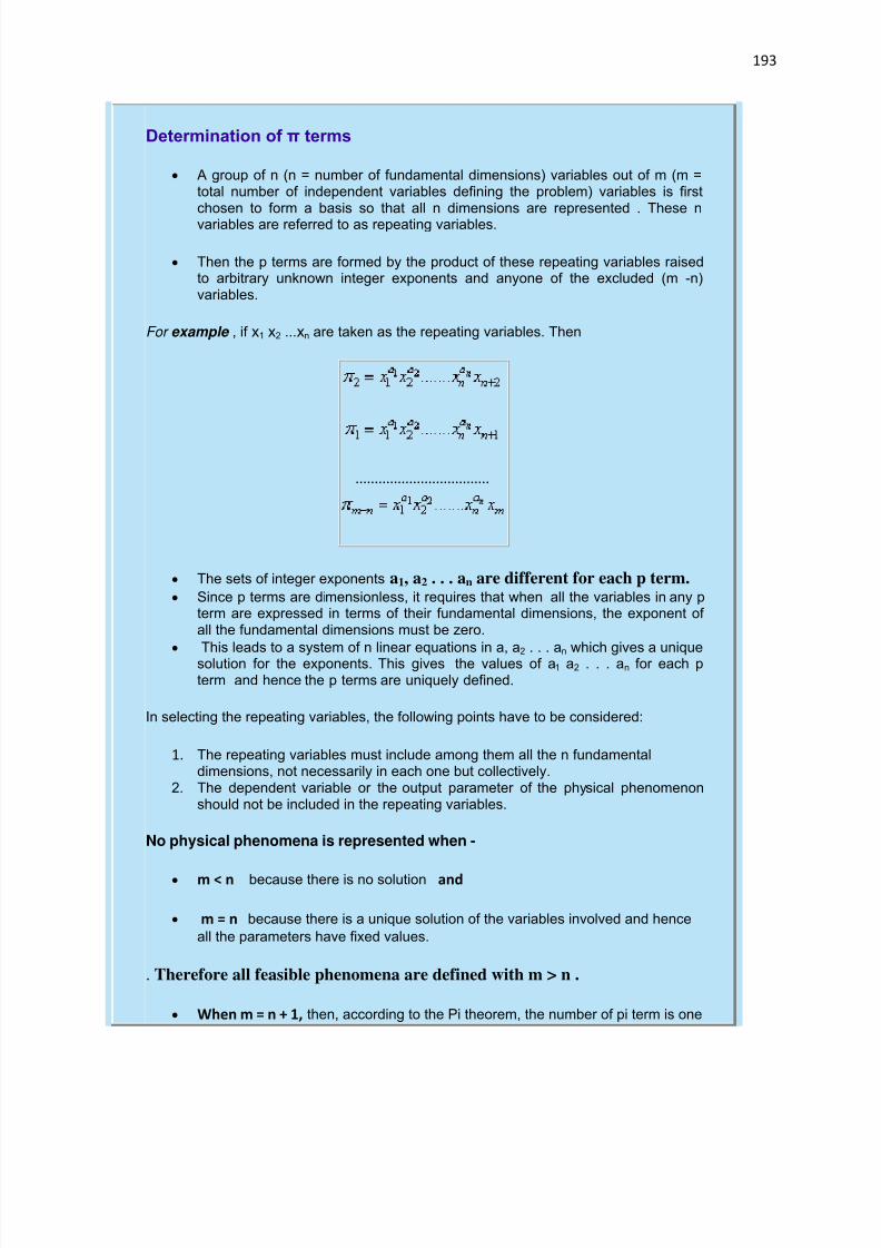
7/29/2019 FLUID MECHANICS LECTURE NOTES
http://slidepdf.com/reader/full/fluid-mechanics-lecture-notes 193/297
193
Determination of π terms
A group of n (n = number of fundamental dimensions) variables out of m (m =total number of independent variables defining the problem) variables is firstchosen to form a basis so that all n dimensions are represented . These nvariables are referred to as repeating variables.
Then the p terms are formed by the product of these repeating variables raisedto arbitrary unknown integer exponents and anyone of the excluded (m -n)variables.
For example , if x1 x2 ...xn are taken as the repeating variables. Then
...................................
The sets of integer exponents a1, a2 . . . an are different for each p term. Since p terms are dimensionless, it requires that when all the variables in any p
term are expressed in terms of their fundamental dimensions, the exponent of all the fundamental dimensions must be zero.
This leads to a system of n linear equations in a, a2
. . . an
which gives a uniquesolution for the exponents. This gives the values of a1 a2 . . . an for each pterm and hence the p terms are uniquely defined.
In selecting the repeating variables, the following points have to be considered:
1. The repeating variables must include among them all the n fundamentaldimensions, not necessarily in each one but collectively.
2. The dependent variable or the output parameter of the physical phenomenonshould not be included in the repeating variables.
No physical phenomena is represented when -
m < n because there is no solution and
m = n because there is a unique solution of the variables involved and hence
all the parameters have fixed values.
. Therefore all feasible phenomena are defined with m > n .
When m = n + 1, then, according to the Pi theorem, the number of pi term is one
7/29/2019 FLUID MECHANICS LECTURE NOTES
http://slidepdf.com/reader/full/fluid-mechanics-lecture-notes 194/297
194
and the phenomenon can be expressed as
where, the non-dimensional term π1 is some specific combination of n + 1 variablesinvolved in the problem.
When m > n+ 1 ,
1. the number of π terms are more than one.
2. A number of choices regarding the repeating variables arise in this case.
Again, it is true that if one of the repeating variables is changed, it results in a differentset of π terms. Therefore the interesting question is which set of repeating variablesis to be chosen , to arrive at the correct set of π terms to describe the problem. Theanswer to this question lies in the fact that different sets of π terms resultingfrom the use of different sets of repeating variables are not independent. Thus,
anyone of such interdependent sets is meaningful in describing the samephysical phenomenon.
From any set of such π terms, one can obtain the other meaningful sets from somecombination of the π terms of the existing set without altering their total numbers (m -n)as fixed by the Pi theorem.
See the Example
Module 4 :
Chapter 8 : Viscous Incompressible Flows
Objectives
Lecture 24
General Viscosity Law
Navier-Stokes Equations
Lecture 25

7/29/2019 FLUID MECHANICS LECTURE NOTES
http://slidepdf.com/reader/full/fluid-mechanics-lecture-notes 195/297
195
A general way of deriving the Navier-Stokes equations from the basic laws of physics
Exact Solution of Navier-Stokes Equations
Lecture 26
Couette Flow
Hagen Poiseuille Flow
Flow between Two Concentric Rotating Cylinders
Lecture 27
Low Reynolds Number Flow Around a Sphere
Theory of Hydrodynamic Lubrication
Exercise Problem
Chapter 8 : Viscous Incompressible Flows
Lecture 25 :
Parallel Flow in a Straight Channel
Consider steady flow between two infinitely broad parallel plates as shown in Fig.25.2.
Flow is independent of any variation in z direction, hence, z dependence is gotten rid of and Eq. (25.11) becomes

7/29/2019 FLUID MECHANICS LECTURE NOTES
http://slidepdf.com/reader/full/fluid-mechanics-lecture-notes 196/297
196
FIG 25.2 Parallel flow in a straight channel
(25.12)
The boundary conditions are at y = b, u = 0; and y = -b, u = O.
From Eq. (25.12), we can write
or
Applying the boundary conditions, the constants are evaluated as
and
So, the solution is
(25.13)
which implies that the velocity profile is parabolic.
Average Velocity and Maximum Velocity
To establish the relationship between the maximum velocity and averagevelocity in the channel, we analyze as follows

7/29/2019 FLUID MECHANICS LECTURE NOTES
http://slidepdf.com/reader/full/fluid-mechanics-lecture-notes 197/297
197
At y = 0, ; this yields
(25.14a)
On the other hand, the average velocity,
or
Finally,(25.14b)
So, or (25.14c)
The shearing stress at the wall for the parallel flow in a channel can bedetermined from the velocity gradient as
Since the upper plate is a "minus y surface", a negative stress acts in the positive xdirection, i.e. to the right.
The local friction coefficient, C f is defined by
(25.14d)
7/29/2019 FLUID MECHANICS LECTURE NOTES
http://slidepdf.com/reader/full/fluid-mechanics-lecture-notes 198/297
198
where is the Reynolds number of flow based on average velocity andthe channel height (2b).
Experiments show that Eq. (25.14d) is valid in the laminar regime of the channel
flow. The maximum Reynolds number value corresponding to fully developed laminar
flow, for which a stable motion will persist, is 2300.
In a reasonably careful experiment, laminar flow can be observed up to even Re= 10,000.
But the value below which the flow will always remain laminar, i.e. the criticalvalue of Re is 2300.
End of Lecture 25!
To start next lecture click next buttonor select from left-hand-side.
Chapter 8 : Viscous Incompressible Flows
Lecture 26 :
Couette Flow
Couette flow is the flow between two parallel plates (Fig. 26.1). Here, one plate is at rest and the other is moving with a velocity U . Let us assume the plates are infinitely large in z direction, so the z dependence is not there.
The governing equation is
f low is independent of any variation in z-direction.
The boundary conditions are ---(i)At y = 0, u = 0 (ii)At y = h, u = U.
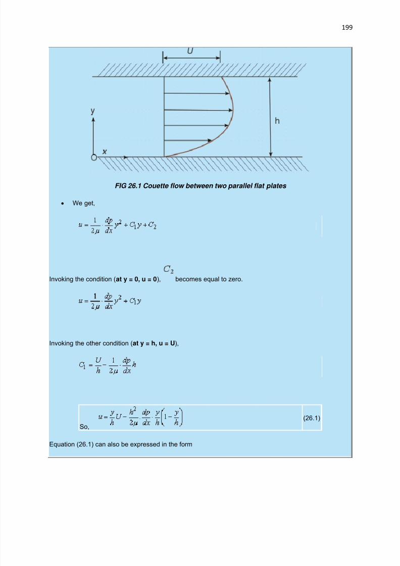
7/29/2019 FLUID MECHANICS LECTURE NOTES
http://slidepdf.com/reader/full/fluid-mechanics-lecture-notes 199/297
199
FIG 26.1 Couette flow between two parallel flat plates
We get,
Invoking the condition (at y = 0, u = 0), becomes equal to zero.
Invoking the other condition (at y = h, u = U),
So,
(26.1)
Equation (26.1) can also be expressed in the form

7/29/2019 FLUID MECHANICS LECTURE NOTES
http://slidepdf.com/reader/full/fluid-mechanics-lecture-notes 200/297
200
or,(26.2a)
Where
,
Equation (26.2a) describes the velocity distribution in non-dimensional form across the channel with P asa parameter known as the non-dimensional pressure gradient .
When P = 0, the velocity distribution across the channel is reduced to
This particular case is known as simple Couette flow.
When P > 0 , i.e. for a negative or favourable pressure gradient in the direction of
motion, the velocity is positive over the whole gap between the channel walls. For negative valueof P ( P < 0 ), there is a positive or adverse pressure gradient in the direction of motion andthe velocity over a portion of channel width can become negative and back flow may occur near the wall which is at rest. Figure 26.2a shows the effect of dragging action of the upper plateexerted on the fluid particles in the channel for different values of pressure gradient.

7/29/2019 FLUID MECHANICS LECTURE NOTES
http://slidepdf.com/reader/full/fluid-mechanics-lecture-notes 201/297
201
FIG 26.2a - Velocity profile for the Couette flow for various values of pressure gradient
Chapter 8 : Viscous Incompressible Flows
Lecture 26 :
Maximum and minimum velocities
The quantitative description of non-dimensional velocity distribution across the channel,depicted by Eq. (26.2a), is shown
in Fig. 26.2b.
The location of maximum or minimum velocity in the channel is found out by
setting =0. From Eq. (26.2a), we can write
Setting gives

7/29/2019 FLUID MECHANICS LECTURE NOTES
http://slidepdf.com/reader/full/fluid-mechanics-lecture-notes 202/297
202
26.2b
It is interesting to note that maximum velocity for P = 1 occurs at y/h = 1 and
equals to U . For P > 1, the maximum velocity occurs at a location .
This means that with P > 1, the fluid particles attain a velocity higher than that of the moving plate at a location somewhere below the moving plate.
For P = -1, the minimum velocity occurs, at . For P < -1, the minimum
velocity occurs at a location .
This means that there occurs a back flow near the fixed plate. The values of maximum and minimum velocities can be determined by substituting the valueof y from Eq. (26.2b) into Eq. (26.2a) as
(26.2c)
FIG 26.2b - Velocity distribution of the Couette flow
Chapter 8 : Viscous Incompressible Flows
Lecture 26 :

7/29/2019 FLUID MECHANICS LECTURE NOTES
http://slidepdf.com/reader/full/fluid-mechanics-lecture-notes 203/297
203
Hagen Poiseuille Flow
Consider fully developed laminar flow through a straight tube of circular cross-section as in Fig. 26.3. Rotational symmetry is considered to make the flow two-dimensional axisymmetric.
Let us take z-axis as the axis of the tube along which all the fluid particlestravel, i.e.
Fig 26.3 - Hagen-Poiseuille flow through a pipe
Now, from continuity equation, we obtain
[ For rotational symmetry, ]
which means
Invoking in the
Navier-Stokes equations, we obtain
(in the z-direction)
(26.3)
For steady flow, the governing equation becomes
(26.4)
The boundary conditions are- (i) At r = 0, is finite and (ii) r = R, yields

7/29/2019 FLUID MECHANICS LECTURE NOTES
http://slidepdf.com/reader/full/fluid-mechanics-lecture-notes 204/297
204
Equation (26.4) can be written as
or,
or,
or,
or,
At r =0, is finite which means A should be equal to zero and at r = R, = 0yields
(26.5)
This shows that the axial velocity profile in a fully developed laminar pipeflow is having parabolic variation along r.
At r = 0, as such,
(26.6a)
The average velocity in the channel,
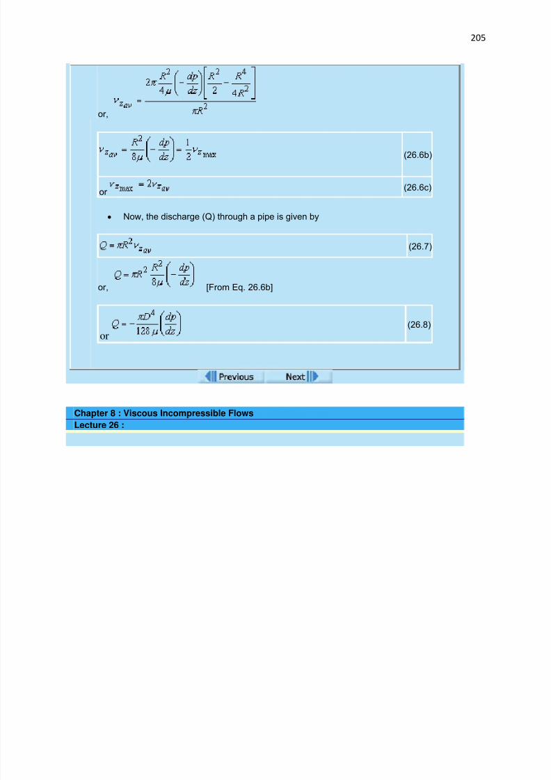
7/29/2019 FLUID MECHANICS LECTURE NOTES
http://slidepdf.com/reader/full/fluid-mechanics-lecture-notes 205/297
205
or,
(26.6b)
or (26.6c)
Now, the discharge (Q) through a pipe is given by
(26.7)
or, [From Eq. 26.6b]
or(26.8)
Chapter 8 : Viscous Incompressible Flows
Lecture 26 :

7/29/2019 FLUID MECHANICS LECTURE NOTES
http://slidepdf.com/reader/full/fluid-mechanics-lecture-notes 206/297
206
Losses and Friction Factors
Over a finite length l , the head loss
(26.11)Combining Eqs (26.10) and (26.11), we get
or
(26.12)
On the other hand, the head loss in a pipe flow is given by Darcy-Weisbachformula as
(26.13)
where "f" is Darcy friction factor . Equations (26.12) and (26.13) yield
which finally gives , where is the Reynolds number.
So, for a fully developed laminar flow, the Darcy (or Moody) friction factor isgiven by
(26.14a)
Alternatively, the skin friction coefficient for Hagen-Poiseuille flow can be expressedby
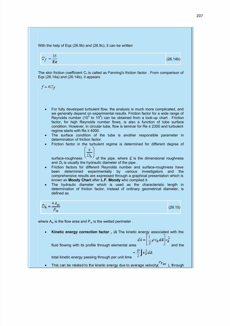
7/29/2019 FLUID MECHANICS LECTURE NOTES
http://slidepdf.com/reader/full/fluid-mechanics-lecture-notes 207/297
207
With the help of Eqs (26.9b) and (26.9c), it can be written
(26.14b)
The skin friction coefficient C f is called as Fanning's friction factor . From comparison of Eqs (26.14a) and (26.14b), it appears
For fully developed turbulent flow, the analysis is much more complicated, and
we generally depend on experimental results. Friction factor for a wide range of Reynolds number (10
4to 10
8) can be obtained from a look-up chart . Friction
factor, for high Reynolds number flows, is also a function of tube surfacecondition. However, in circular tube, flow is laminar for Re ≤ 2300 and turbulentregime starts with Re ≥ 4000.
The surface condition of the tube is another responsible parameter indetermination of friction factor.
Friction factor in the turbulent regime is determined for different degree of
surface-roughness of the pipe, where is the dimensional roughnessand D h is usually the hydraulic diameter of the pipe .
Friction factors for different Reynolds number and surface-roughness have
been determined experimentally by various investigators and thecomprehensive results are expressed through a graphical presentation which isknown as Moody Chart after L.F. Moody who compiled it.
The hydraulic diameter which is used as the characteristic length indetermination of friction factor, instead of ordinary geometrical diameter, isdefined as
(26.15)
where Aw is the flow area and Pw is the wetted perimeter .
Kinetic energy correction factor , The kinetic energy associated with the
fluid flowing with its profile through elemental area and the
total kinetic energy passing through per unit time .
This can be related to the kinetic energy due to average velocity( ), through
7/29/2019 FLUID MECHANICS LECTURE NOTES
http://slidepdf.com/reader/full/fluid-mechanics-lecture-notes 208/297
208
a correction factor, α as
or
Here, for Hagen-Poiseuille flow,
(26.16)
Module 5 :
Chapter 9 : Laminar Boundary Layers
Objectives
Lecture 28
Introduction to Boundary Layer Equations
Blasius Flow over a flat plate
Lecture 29
Wall shear and boundary layer thickness
Momentum-Integral equations for the boundary layer
Lecture 30
Karman-Pohlhausen approximate method for solution of momentum integral equation over a flat plate
7/29/2019 FLUID MECHANICS LECTURE NOTES
http://slidepdf.com/reader/full/fluid-mechanics-lecture-notes 209/297
209
Integral method for non-zero pressure gradient flows
Lecture 31
Entry flow in a ductControl of boundary layer separation
Mechanisms of boundary layer transition
Chapter 9 : Laminar Boundary Layers
Lecture 28 :
Introduction
The boundary layer of a flowing fluid is the thin layer close to the wall
In a flow field, viscous stresses are very prominent within this layer.
Although the layer is thin, it is very important to know the details of flow within it.
The main-flow velocity within this layer tends to zero while approaching thewall (no-slip condition).
Also the gradient of this velocity component in a direction normal to the surfaceis large as compared to the gradient in the streamwise direction.
Chapter 9 : Laminar Boundary Layers
Lecture 28 :

7/29/2019 FLUID MECHANICS LECTURE NOTES
http://slidepdf.com/reader/full/fluid-mechanics-lecture-notes 210/297
210
Boundary Layer Equations
In 1904, Ludwig Prandtl, the well known German scientist, introduced the concept of boundarylayer and derived the equations for boundary layer flow by correct reduction of Navier-Stokesequations.
He hypothesized that for fluids having relatively small viscosity, the effect of internalfriction in the fluid is significant only in a narrow region surrounding solid boundaries orbodies over which the fluid flows.
Thus, close to the body is the boundary layer where shear stresses exert an increasinglylarger effect on the fluid as one moves from free stream towards the solid boundary.
However, outside the boundary layer where the effect of the shear stresses on the flow is
small compared to values inside the boundary layer (since the velocity gradient isnegligible),---------
1. the fluid particles experience no vorticity and therefore, 2. the flow is similar to a potential flow.
Hence, the surface at the boundary layer interface is a rather fictitious one, that divides
rotational and irrotational flow. Fig 28.1 shows Prandtl's model regarding boundary layer flow.
Hence with the exception of the immediate vicinity of the surface, the flow is frictionless (inviscid)
and the velocity is U (the potential velocity).
In the region, very near to the surface (in the thin layer), there is friction in the flow which signifiesthat the fluid is retarded until it adheres to the surface (no-slip condition).
The transition of the mainstream velocity from zero at the surface (with respect to the surface) tofull magnitude takes place across the boundary layer.
About the boundary layer
Boundary layer thickness is which is a function of the coordinate direction x .
The thickness is considered to be very small compared to the characteristic length L of the
domain.
In the normal direction, within this thin layer, the gradient is very large compared to
the gradient in the flow direction .
Now we take up the Navier-Stokes equations for : steady, two dimensional, laminar, incompressible
flows.
Considering the Navier-Stokes equations together with the equation of continuity, the followingdimensional form is obtained.
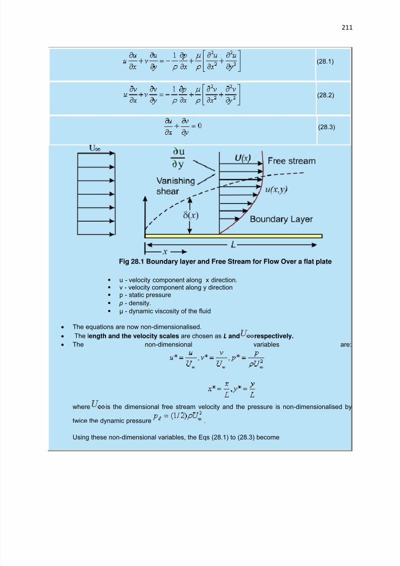
7/29/2019 FLUID MECHANICS LECTURE NOTES
http://slidepdf.com/reader/full/fluid-mechanics-lecture-notes 211/297
211
(28.1)
(28.2)
(28.3)
Fig 28.1 Boundary layer and Free Stream for Flow Over a flat plate
u - velocity component along x direction. v - velocity component along y direction
p - static pressure ρ - density.
μ - dynamic viscosity of the fluid
The equations are now non-dimensionalised.
The length and the velocity scales are chosen as L and respectively.
The non-dimensional variables are:
where is the dimensional free stream velocity and the pressure is non-dimensionalised by
twice the dynamic pressure .
Using these non-dimensional variables, the Eqs (28.1) to (28.3) become
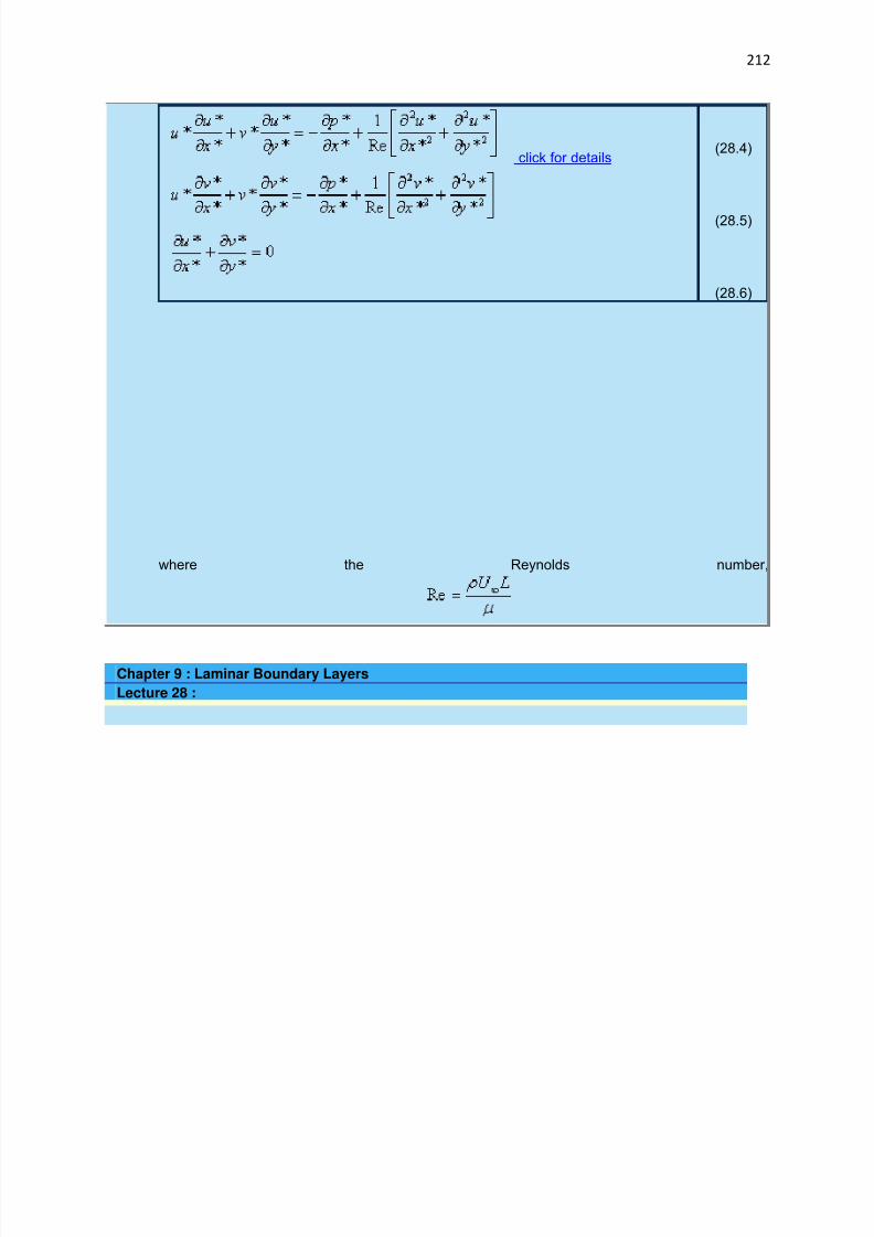
7/29/2019 FLUID MECHANICS LECTURE NOTES
http://slidepdf.com/reader/full/fluid-mechanics-lecture-notes 212/297
212
where the Reynolds number,
click for details(28.4)
(28.5)
(28.6)
Chapter 9 : Laminar Boundary Layers
Lecture 28 :

7/29/2019 FLUID MECHANICS LECTURE NOTES
http://slidepdf.com/reader/full/fluid-mechanics-lecture-notes 213/297
213
Order of Magnitude Analysis
Let us examine what happens to the u velocity as we go across the boundary layer. At the wall the u velocity is zero [ with respect to the wall and absolute zero for a stationarywall (which is normally implied if not stated otherwise)].The value of u on the inviscid side, that is on the free stream side beyond the boundarylayer is U .
For the case of external flow over a flat plate, this U is equal to .
Based on the above, we can identify the following scales for the boundary layer variables:
Variable Dimensional scale Non-dimensional scale
The symbol describes a value much smaller than 1.
Now we analyse equations 28.4 - 28.6, and look at the order of magnitude of each individualterm
Eq 28.6 - the continuity equation
One general rule of incompressible fluid mechanics is that we are not allowed to drop any termfrom the continuity equation.
From the scales of boundary layer variables, the derivative is of the order 1.
The second term in the continuity equation should also be of the
order 1.The reason being has to be of the order because becomes
at its maximum.
Eq 28.4 - x direction momentum equation
Inertia terms are of the order 1.
is of the order 1
is of the order .
However after multiplication with 1/Re, the sum of the two second order derivatives should produce atleast one term which is of the same order of magnitude as the inertia terms. This is possible only
if the Reynolds number (Re) is of the order of .
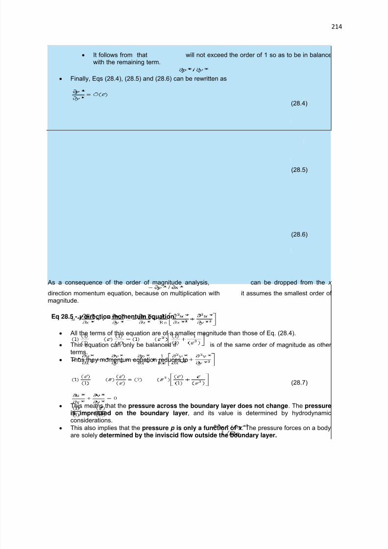
7/29/2019 FLUID MECHANICS LECTURE NOTES
http://slidepdf.com/reader/full/fluid-mechanics-lecture-notes 214/297
214
It follows from that will not exceed the order of 1 so as to be in balancewith the remaining term.
Finally, Eqs (28.4), (28.5) and (28.6) can be rewritten as
(28.4)
(28.5)
(28.6)
As a consequence of the order of magnitude analysis, can be dropped from the x
direction momentum equation, because on multiplication with it assumes the smallest order of magnitude.
Eq 28.5 - y direction momentum equation.
All the terms of this equation are of a smaller magnitude than those of Eq. (28.4).
This equation can only be balanced if is of the same order of magnitude as other terms.
Thus they momentum equation reduces to
(28.7)
This means that the pressure across the boundary layer does not change. The pressureis impressed on the boundary layer, and its value is determined by hydrodynamicconsiderations.
This also implies that the pressure p is only a function of x . The pressure forces on a bodyare solely determined by the inviscid flow outside the boundary layer.
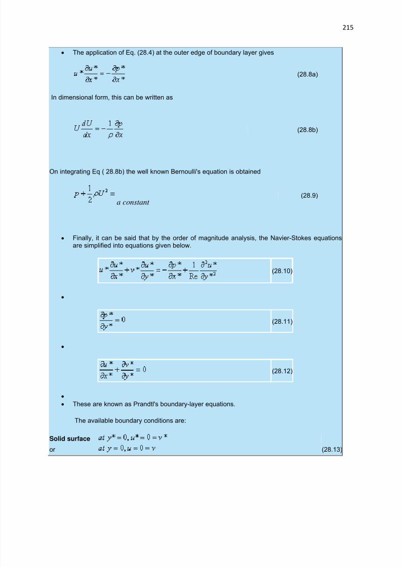
7/29/2019 FLUID MECHANICS LECTURE NOTES
http://slidepdf.com/reader/full/fluid-mechanics-lecture-notes 215/297
215
The application of Eq. (28.4) at the outer edge of boundary layer gives
(28.8a)
In dimensional form, this can be written as
(28.8b)
On integrating Eq ( 28.8b) the well known Bernoulli's equation is obtained
a constant (28.9)
Finally, it can be said that by the order of magnitude analysis, the Navier-Stokes equationsare simplified into equations given below.
(28.10)
(28.11)
(28.12)
These are known as Prandtl's boundary-layer equations.
The available boundary conditions are:
Solid surface
or (28.13)

7/29/2019 FLUID MECHANICS LECTURE NOTES
http://slidepdf.com/reader/full/fluid-mechanics-lecture-notes 216/297

7/29/2019 FLUID MECHANICS LECTURE NOTES
http://slidepdf.com/reader/full/fluid-mechanics-lecture-notes 217/297
217
Boundary Layer Coordinates
The boundary layer equations derived are in Cartesian coordinates.
The Velocity components u and v represent x and y direction velocitiesrespectively.
For objects with small curvature, these equations can be used with - x coordinate : streamwise direction y coordinate : normal component
They are called Boundary Layer Coordinates.
Application of Boundary Layer Theory
The Boundary-Layer Theory is not valid beyond the point of separation.
At the point of separation, boundary layer thickness becomes quite large for thethin layer approximation to be valid.
It is important to note that boundary layer theory can be used to locate the point
of seperation itself. In applying the boundary layer theory although U is the free-stream velocity at
the outer edge of the boundary layer, it is interpreted as the fluid velocity at thewall calculated from inviscid flow considerations ( known as Potential WallVelocity)
Mathematically, application of the boundary - layer theory converts thecharacter of governing Navier-Stroke equations from elliptic to parabolic
This allows the marching in flow direction, as the solution at any location isindependent of the conditions farther downstream.
Chapter 9 : Laminar Boundary Layers
Lecture 28 :
Blasius Flow Over A Flat Plate
The classical problem considered by H. Blasius was1. Two-dimensional, steady, incompressible flow over a flat plate at zero
angle of incidence with respect to the uniform stream of velocity .2. The fluid extends to infinity in all directions from the plate.
The physical problem is already illustrated in Fig. 28.1
Blasius wanted to determine(a) the velocity field solely within the boundary layer,
(b) the boundary layer thickness ,(c) the shear stress distribution on the plate, and(d) the drag force on the plate.

7/29/2019 FLUID MECHANICS LECTURE NOTES
http://slidepdf.com/reader/full/fluid-mechanics-lecture-notes 218/297
218
The Prandtl boundary layer equations in the case under consideration are
(28.15)
The boundary conditions are
(28.16)
Note that the substitution of the term in the original boundary layer
momentum equation in terms of the free stream velocity produceswhich is equal to zero.
Hence the governing Eq. (28.15) does not contain any pressure-gradient term.
However, the characteristic parameters of this problem are that is,
This relation has five variables .
It involves two dimensions, length and time. Thus it can be reduced to a dimensionless relation in terms of (5-2) =3quantities ( Buckingham Pi Theorem)
Thus a similarity variables can be used to find the solution
Such flow fields are called self-similar flow field .
Chapter 9 : Laminar Boundary Layers
Lecture 28 :
Law of Similarity for Boundary Layer Flows
It states that the u component of velocity with two velocity profiles of u(x,y) atdifferent x locations differ only by scale factors in u and y .
Therefore, the velocity profiles u(x,y) at all values of x can be made congruent if theyare plotted in coordinates which have been made dimensionless with reference to
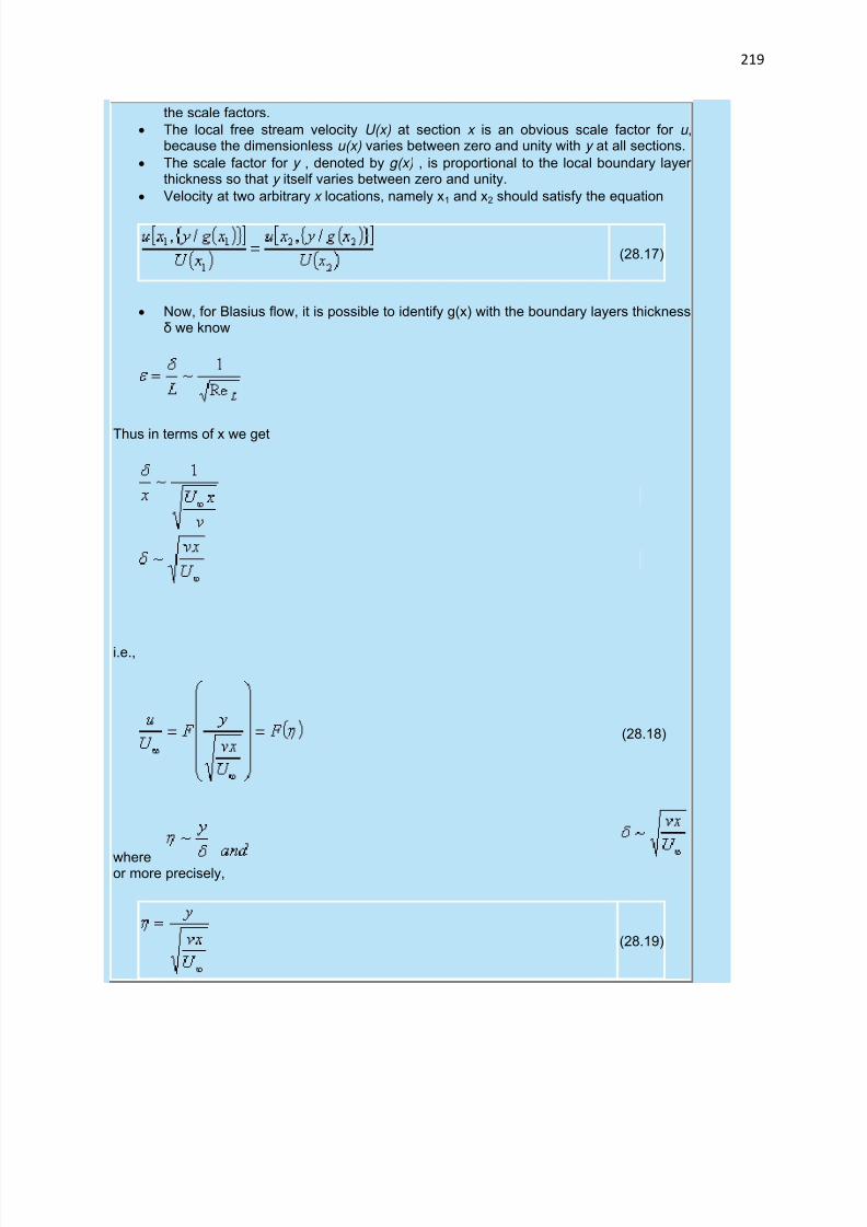
7/29/2019 FLUID MECHANICS LECTURE NOTES
http://slidepdf.com/reader/full/fluid-mechanics-lecture-notes 219/297
219
the scale factors.
The local free stream velocity U(x) at section x is an obvious scale factor for u ,because the dimensionless u(x) varies between zero and unity with y at all sections.
The scale factor for y , denoted by g(x) , is proportional to the local boundary layer thickness so that y itself varies between zero and unity.
Velocity at two arbitrary x locations, namely x1 and x2 should satisfy the equation
(28.17)
Now, for Blasius flow, it is possible to identify g(x) with the boundary layers thicknessδ we know
Thus in terms of x we get
i.e.,
(28.18)
whereor more precisely,
(28.19)

7/29/2019 FLUID MECHANICS LECTURE NOTES
http://slidepdf.com/reader/full/fluid-mechanics-lecture-notes 220/297
220
The stream function can now be obtained in terms of the velocity components as
or
(28.20)
where D is a constant. Also and the constant of integration is zero if thestream function at the solid surface is set equal to zero.
Now, the velocity components and their derivatives are:
(28.21a)
or
(28.21b)
(28.21c)
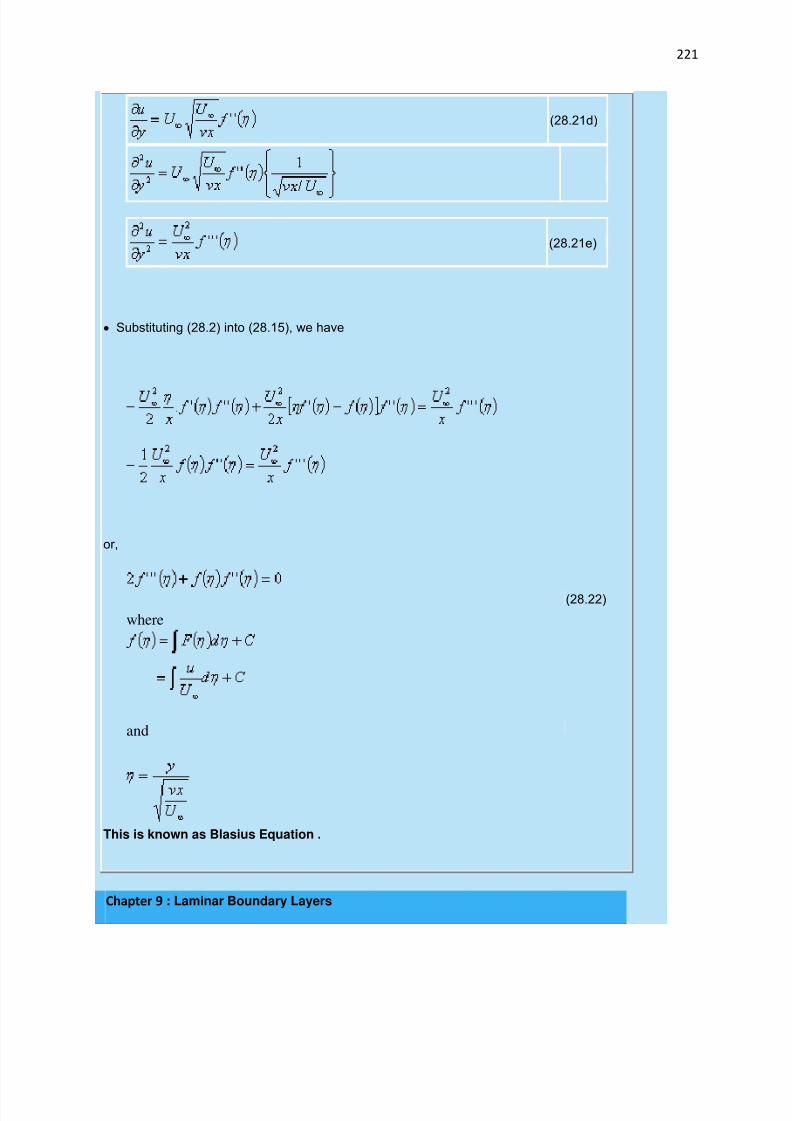
7/29/2019 FLUID MECHANICS LECTURE NOTES
http://slidepdf.com/reader/full/fluid-mechanics-lecture-notes 221/297
221
(28.21d)
(28.21e)
Substituting (28.2) into (28.15), we have
or,
where
(28.22)
and
This is known as Blasius Equation .
Chapter 9 : Laminar Boundary Layers
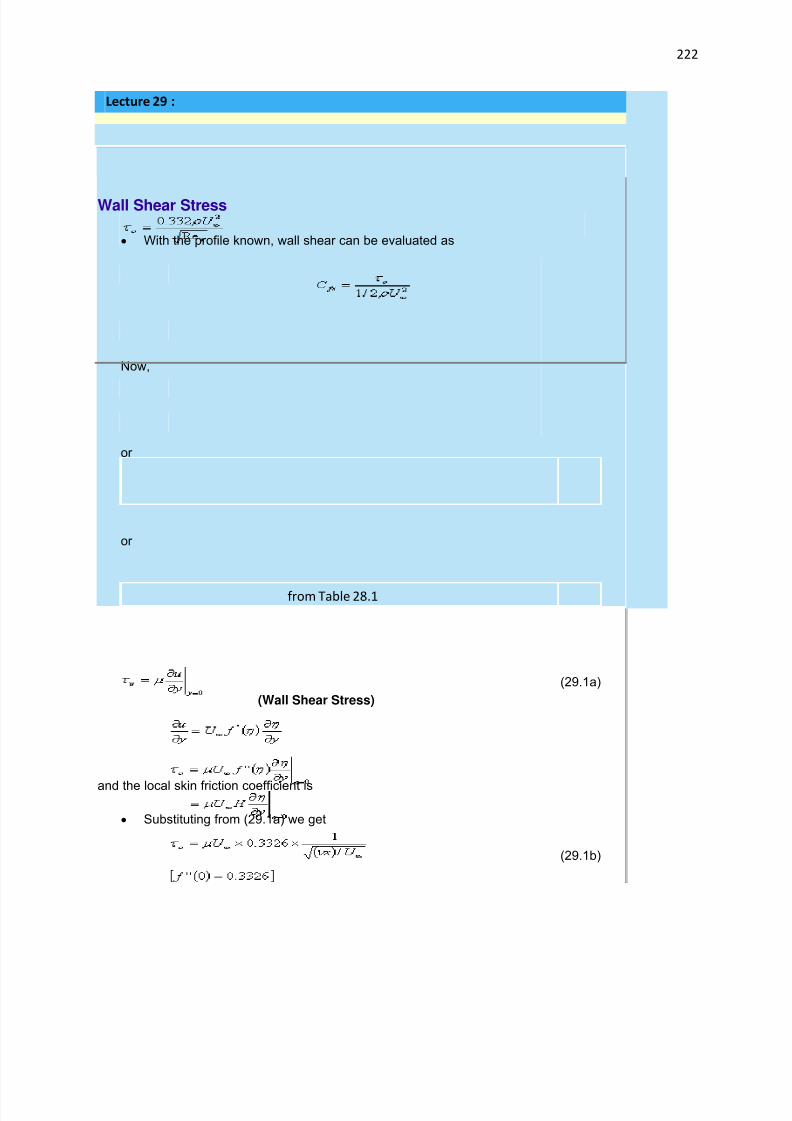
7/29/2019 FLUID MECHANICS LECTURE NOTES
http://slidepdf.com/reader/full/fluid-mechanics-lecture-notes 222/297
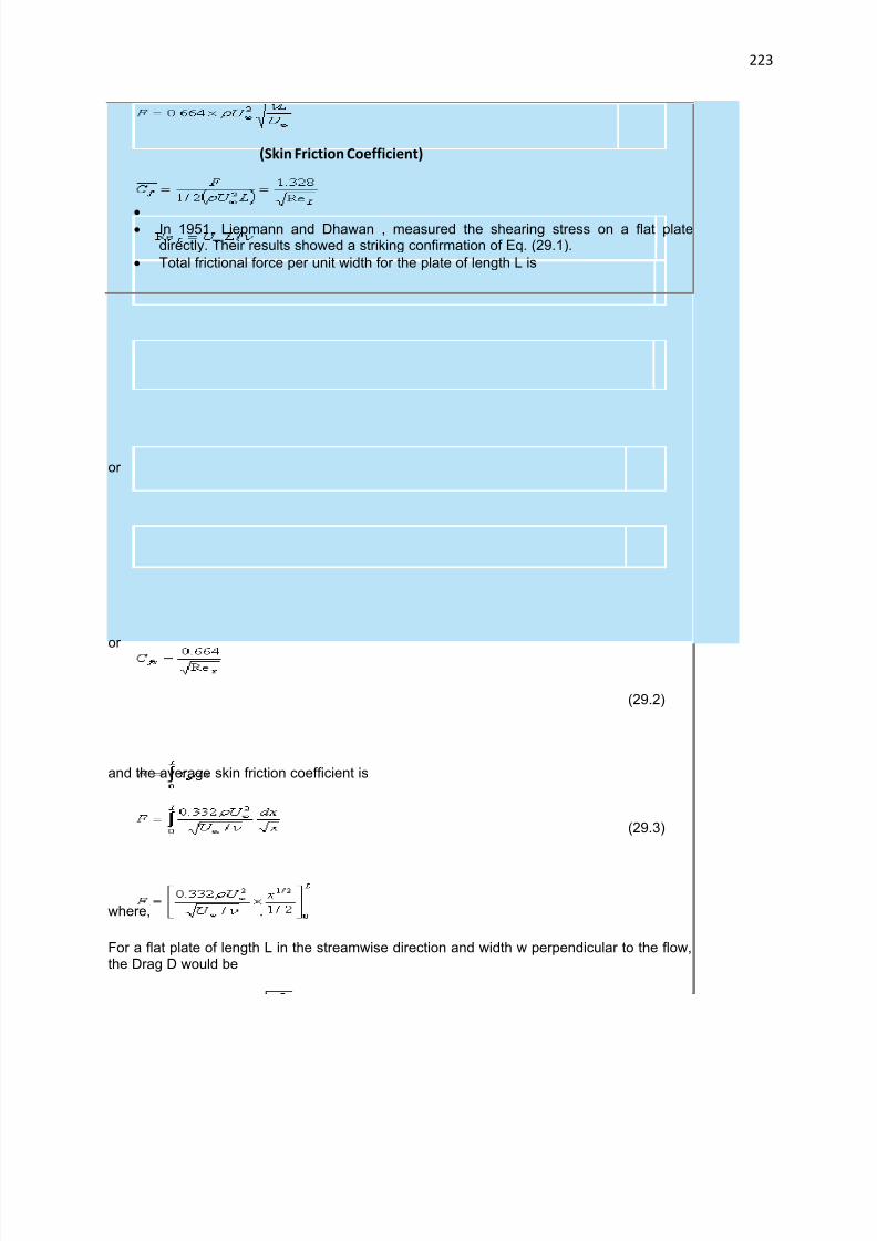
7/29/2019 FLUID MECHANICS LECTURE NOTES
http://slidepdf.com/reader/full/fluid-mechanics-lecture-notes 223/297
223
(Skin Friction Coefficient)
In 1951, Liepmann and Dhawan , measured the shearing stress on a flat platedirectly. Their results showed a striking confirmation of Eq. (29.1).
Total frictional force per unit width for the plate of length L is
or
or
(29.2)
and the average skin friction coefficient is
(29.3)
where, .
For a flat plate of length L in the streamwise direction and width w perpendicular to the flow,the Drag D would be
7/29/2019 FLUID MECHANICS LECTURE NOTES
http://slidepdf.com/reader/full/fluid-mechanics-lecture-notes 224/297
224
(29.4)
Let us do an Example
Chapter 9 : Laminar Boundary LayersLecture 29 :
Boundary Layer Thickness
Since , it is customary to select the boundary layer
thickness as that point where approaches 0.99.
From Table 28.1, reaches 0.99 at η= 5.0 and we can write
(29.5)
However, the aforesaid definition of boundary layer thickness is somewhat arbitrary, a
physically more meaningful measure of boundary layer estimation is expressed throughdisplacement thickness .

7/29/2019 FLUID MECHANICS LECTURE NOTES
http://slidepdf.com/reader/full/fluid-mechanics-lecture-notes 225/297
225
Fig. 29.1 (Displacement thickness) (b) Momentum thickness
Displacement thickness : It is defined as the distance by which the externalpotential flow is displaced outwards due to the decrease in velocity in the boundary
layer.
Therefore,
(29.6)
Substituting the values of and from Eqs (28.21a) and (28.19) into Eq.(29.6),we obtain
or,
(29.7)
Following the analogy of the displacement thickness, a momentum thickness may be defined.
Momentum thickness ( ): It is defined as the loss of momentum in the boundary layer ascompared with that of potential flow. Thus
7/29/2019 FLUID MECHANICS LECTURE NOTES
http://slidepdf.com/reader/full/fluid-mechanics-lecture-notes 226/297
226
(29.8)
With the substitution of and from Eg. (28.21a) and (28.19), we can evaluate
numerically the value of for a flat plate as
(29.9)
The relationships between have been shown in Fig. 29.1.
Chapter 9 : Laminar Boundary Layers
Lecture 29 :

7/29/2019 FLUID MECHANICS LECTURE NOTES
http://slidepdf.com/reader/full/fluid-mechanics-lecture-notes 227/297
227
Momentum-Integral Equations For The Boundary Layer
To employ boundary layer concepts in real engineering designs, we needapproximate methods that would quickly lead to an answer even if the accuracy issomewhat less.
Karman and Pohlhausen devised a simplified method by satisfying only theboundary conditions of the boundary layer flow rather than satisfying Prandtl'sdifferential equations for each and every particle within the boundary layer. We shalldiscuss this method herein.
Consider the case of steady, two-dimensional and incompressible flow, i.e. we shallrefer to Eqs (28.10) to (28.14). Upon integrating the dimensional form of Eq. (28.10)with respect to y = 0 (wall) to y = δ (where δ signifies the interface of the free streamand the boundary layer), we obtain
or,
(29.10)
The second term of the left hand side can be expanded as
or, by continuity equation
or,
(29.11)
Substituting Eq. (29.11) in Eq. (29.10) we obtain
(29.12)
Substituting the relation between and the free stream velocity for the inviscid

7/29/2019 FLUID MECHANICS LECTURE NOTES
http://slidepdf.com/reader/full/fluid-mechanics-lecture-notes 228/297
228
zone in Eq. (29.12) we get
which is reduced to
Since the integrals vanish outside the boundary layer, we are allowed to increase the
integration limit to infinity (i.e . )
or,
(29.13)
Substituting Eq. (29.6) and (29.7) in Eq. (29.13) we obtain
(29.14)
where is the displacement thickness
is momentum thickness
Equation (29.14) is known as momentum integral equation for two dimensionalincompressible laminar boundary layer. The same remains valid for turbulent boundarylayers as well.
7/29/2019 FLUID MECHANICS LECTURE NOTES
http://slidepdf.com/reader/full/fluid-mechanics-lecture-notes 229/297
229
Needless to say, the wall shear stress will be different for laminar and turbulentflows.
The term signifies space-wise acceleration of the free stream. Existence of this term means that free stream pressure gradient is present in the flow direction.
For example, we get finite value of outside the boundary layer in theentrance region of a pipe or a channel. For external flows, the existence of
depends on the shape of the body.
During the flow over a flat plate, and the momentum integral equationis reduced to
(29.15)
Chapter 9 : Laminar Boundary Layers
Lecture 29 :
7/29/2019 FLUID MECHANICS LECTURE NOTES
http://slidepdf.com/reader/full/fluid-mechanics-lecture-notes 230/297
230
Seperation of Boundary Layer
It has been observed that the flow is reversed at the vicinity of the wall under certain conditions.
The phenomenon is termed as separation of boundary layer.
Separation takes place due to excessive momentum loss near the wall in aboundary layer trying to move downstream against increasing pressure, i.e.,
, which is called adverse pressure gradient .
Figure 29.2 shows the flow past a circular cylinder, in an infinite medium.
1. Up to , the flow area is like a constricted passage and theflow behaviour is like that of a nozzle.
2. Beyond the flow area is diverged, therefore, the flowbehaviour is much similar to a diffuser
This dictates the inviscid pressure distribution on the cylinder which is shown by afirm line in Fig. 29.2.
Here
: pressure in the free stream
: velocity in the free stream and
: is the local pressure on the cylinder.
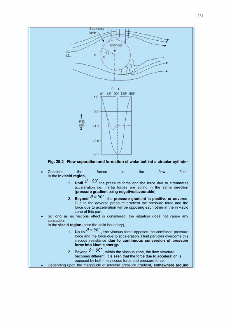
7/29/2019 FLUID MECHANICS LECTURE NOTES
http://slidepdf.com/reader/full/fluid-mechanics-lecture-notes 231/297
231
Fig. 29.2 Flow separation and formation of wake behind a circular cylinder
Consider the forces in the flow field.In the inviscid region,
1. Until the pressure force and the force due to streamwiseacceleration i.e. inertia forces are acting in the same direction(pressure gradient being negative/favourable)
2. Beyond , the pressure gradient is positive or adverse.Due to the adverse pressure gradient the pressure force and theforce due to acceleration will be opposing each other in the in viscidzone of this part.
So long as no viscous effect is considered, the situation does not cause anysensation.In the viscid region (near the solid boundary),
1. Up to , the viscous force opposes the combined pressureforce and the force due to acceleration. Fluid particles overcome thisviscous resistance due to continuous conversion of pressureforce into kinetic energy.
2. Beyond , within the viscous zone, the flow structurebecomes different. It is seen that the force due to acceleration isopposed by both the viscous force and pressure force.
Depending upon the magnitude of adverse pressure gradient, somewhere around
7/29/2019 FLUID MECHANICS LECTURE NOTES
http://slidepdf.com/reader/full/fluid-mechanics-lecture-notes 232/297
232
, the fluid particles, in the boundary layer are separated from the walland driven in the upstream direction. However, the far field external stream pushesback these separated layers together with it and develops a broad pulsating wakebehind the cylinder.
The mathematical explanation of flow-separation : The point of separation maybe defined as the limit between forward and reverse flow in the layer very close tothe wall, i.e., at the point of separation
(29.16)
This means that the shear stress at the wall, . But at this point, the adversepressure continues to exist and at the downstream of this point the flow acts in areverse direction resulting in a back flow.
We can also explain flow separation using the argument about the second derivative
of velocity u at the wall. From the dimensional form of the momentum at the wall,where u = v = 0 , we can write
(29.17)
Consider the situation due to a favourable pressure gradient where we
have,
1. . (From Eq. (29.17))
2. As we proceed towards the free stream, the velocity u approaches
asymptotically, so decreases at a continuously lesser rate in y direction.
3. This means that remains less than zero near the edge of theboundary layer.
4. The curvature of a velocity profile is always negative as shown in
(Fig. 29.3a) Consider the case of adverse pressure gradient,
1. At the boundary, the curvature of the profile must be positive (since
).2. Near the interface of boundary layer and free stream the previous argument
regarding and still holds good and the curvature isnegative.
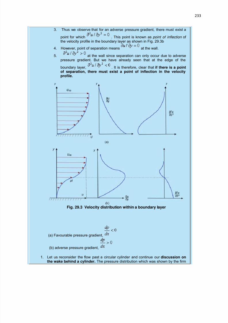
7/29/2019 FLUID MECHANICS LECTURE NOTES
http://slidepdf.com/reader/full/fluid-mechanics-lecture-notes 233/297
233
3. Thus we observe that for an adverse pressure gradient, there must exist a
point for which . This point is known as point of inflection of the velocity profile in the boundary layer as shown in Fig. 29.3b
4. However, point of separation means at the wall.
5. at the wall since separation can only occur due to adversepressure gradient. But we have already seen that at the edge of the
boundary layer, . It is therefore, clear that if there is a pointof separation, there must exist a point of inflection in the velocityprofile.
Fig. 29.3 Velocity distribution within a boundary layer
(a) Favourable pressure gradient,
(b) adverse pressure gradient,
1. Let us reconsider the flow past a circular cylinder and continue our discussion onthe wake behind a cylinder. The pressure distribution which was shown by the firm
7/29/2019 FLUID MECHANICS LECTURE NOTES
http://slidepdf.com/reader/full/fluid-mechanics-lecture-notes 234/297
234
line in Fig. 21.5 is obtained from the potential flow theory. However. somewhere near
(in experiments it has been observed to be at ) . the boundarylayer detaches itself from the wall.
2. Meanwhile, pressure in the wake remains close to separation-point-pressure since the eddies (formed as a consequence of the retarded layers being carriedtogether with the upper layer through the action of shear) cannot convert rotational
kinetic energy into pressure head. The actual pressure distribution is shown by thedotted line in Fig. 29.3.
3. Since the wake zone pressure is less than that of the forward stagnation point(pressure at point A in Fig. 29.3), the cylinder experiences a drag force which isbasically attributed to the pressure difference.
The drag force, brought about by the pressure difference is known as form drag whereas the shear stress at the wall gives rise to skin friction drag .Generally, these two drag forces together are responsible for resultant drag on abody
End of Lecture 29!
To start next lecture click next buttonor select from left-hand-side.
Chapter 9 : Laminar Boundary Layers
Lecture 30 :

7/29/2019 FLUID MECHANICS LECTURE NOTES
http://slidepdf.com/reader/full/fluid-mechanics-lecture-notes 235/297
235
Karman-Pohlhausen Approximate Method For Solution Of MomentumIntegral Equation Over A Flat Plate
The basic equation for this method is obtained by integrating the x direction
momentum equation (boundary layer momentum equation) with respect to y fromthe wall (at y = 0) to a distance which is assumed to be outside the boundarylayer. Using this notation, we can rewrite the Karman momentum integral equationas
(30.1)
The effect of pressure gradient is described by the second term on the left handside. For pressure gradient surfaces in external flow or for the developing sections ininternal flow, this term contributes to the pressure gradient.
We assume a velocity profile which is a polynomial of . being a formof similarity variable , implies that with the growth of boundary layer as
distance x varies from the leading edge, the velocity profile remainsgeometrically similar.
We choose a velocity profile in the form
(30.2)
In order to determine the constants we shall prescribe the
following boundary conditions
(30.3a)
(30.3b)
at
(30.3c)
at
(30.3d)
These requirements will

7/29/2019 FLUID MECHANICS LECTURE NOTES
http://slidepdf.com/reader/full/fluid-mechanics-lecture-notes 236/297
236
yield respectivelyFinally, we obtain the following values for the coefficients in Eq. (30.2),
and the velocity profile becomes
(30.4)
For flow over a flat plate, and the governing Eq.(30.1) reduces to
(30.5)
Again from Eq. (29.8), the momentum thickness is
The wall shear stress is given by
Substituting the values of and in Eq. (30.5) we get,
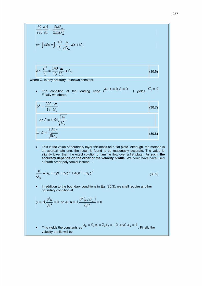
7/29/2019 FLUID MECHANICS LECTURE NOTES
http://slidepdf.com/reader/full/fluid-mechanics-lecture-notes 237/297
237
(30.6)
where C1 is any arbitrary unknown constant.
The condition at the leading edge ( ) yieldsFinally we obtain,
(30.7)
(30.8)
This is the value of boundary layer thickness on a flat plate. Although, the method is
an approximate one, the result is found to be reasonably accurate. The value isslightly lower than the exact solution of laminar flow over a flat plate . As such, theaccuracy depends on the order of the velocity profile. We could have have useda fourth order polynomial instead --
(30.9)
In addition to the boundary conditions in Eq. (30.3), we shall require another boundary condition at
This yields the constants as . Finally the
velocity profile will be
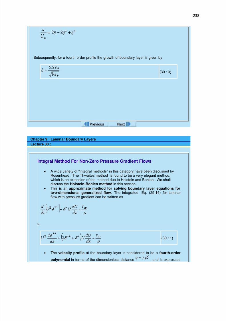
7/29/2019 FLUID MECHANICS LECTURE NOTES
http://slidepdf.com/reader/full/fluid-mechanics-lecture-notes 238/297
238
Subsequently, for a fourth order profile the growth of boundary layer is given by
(30.10)
Chapter 9 : Laminar Boundary Layers
Lecture 30 :
Integral Method For Non-Zero Pressure Gradient Flows
A wide variety of "integral methods" in this category have been discussed byRosenhead . The Thwaites method is found to be a very elegant method,which is an extension of the method due to Holstein and Bohlen . We shalldiscuss the Holstein-Bohlen method in this section.
This is an approximate method for solving boundary layer equations fortwo-dimensional generalized flow. The integrated Eq. (29.14) for laminar flow with pressure gradient can be written as
or
(30.11)
The velocity profile at the boundary layer is considered to be a fourth-order
polynomial in terms of the dimensionless distance , and is expressed

7/29/2019 FLUID MECHANICS LECTURE NOTES
http://slidepdf.com/reader/full/fluid-mechanics-lecture-notes 239/297
239
as
The boundary conditions are
A dimensionless quantity, known as shape factor is introduced as
(30.12)
The following relations are obtained
Now, the velocity profile can be expressed as
(30.13)
where
The shear stress is given by
(30.14)
We use the following dimensionless parameters,
(30.15)

7/29/2019 FLUID MECHANICS LECTURE NOTES
http://slidepdf.com/reader/full/fluid-mechanics-lecture-notes 240/297
240
(30.16)
(30.17)
The integrated momentum Eq. (30.10) reduces to
(30.18)
The parameter L is related to the skin friction
The parameter K is linked to the pressure gradient.
If we take K as the independent variable . L and H can be shown to be thefunctions of K since
(30.19)
(30.20)
(30.21)
Therefore,
The right-hand side of Eq. (30.18) is thus a function of K alone. Walz pointedout that this function can be approximated with a good degree of accuracy by alinear function of K so that

7/29/2019 FLUID MECHANICS LECTURE NOTES
http://slidepdf.com/reader/full/fluid-mechanics-lecture-notes 241/297
241
[Walz's approximation]
Equation (30.18) can now be written as
Solution of this differential equation for the dependent variable subject tothe boundary condition U = 0 when x = 0 , gives
With a = 0.47 and b = 6. the approximation is particularly close betweenthe stagnation point and the point of maximum velocity.
Finally the value of the dependent variable is
(30.22)
By taking the limit of Eq. (30.22), according to L'Hopital's rule, it can be shownthat
This corresponds to K = 0.0783.
Note that is not equal to zero at the stagnation point. If isdetermined from Eq. (30.22), K(x) can be obtained from Eq. (30.16).
Table 30.1 gives the necessary parameters for obtaining results, such as
velocity profile and shear stress The approximate method can be appliedsuccessfully to a wide range of problems.
Table 30.1 Auxiliary functions after Holstein and Bohlen
K
12 0.0948 2.250 0.356
10 0.0919 2.260 0.351
8 0.0831 2.289 0.340
7.6 0.0807 2.297 0.337

7/29/2019 FLUID MECHANICS LECTURE NOTES
http://slidepdf.com/reader/full/fluid-mechanics-lecture-notes 242/297
242
7.2 0.0781 2.305 0.333
7.0 0.0767 2.309 0.331
6.6 0.0737 2.318 0.328
6.2 0.0706 2.328 0.324
5.0 0.0599 2.361 0.310
3.0 0.0385 2.427 0.283
1.0 0.0135 2.508 0.252
0 0 2.554 0.235
-1 -0.0140 2.604 0.217
-3 -0.0429 2.716 0.179
-5 -0.0720 2.847 0.140
-7 -0.0999 2.999 0.100-9 -0.1254 3.176 0.059
-11 -0.1474 3.383 0.019
-12 -0.1567 3.500 0
0 0 0 0
0.2 0.00664 0.006641 0.006641
0.4 0.02656 0.13277 0.132770.8 0.10611 0.26471 0.26471
1.2 0.23795 0.39378 0.39378
1.6 0.42032 0.51676 0.51676
2.0 0.65003 0.62977 0.62977
2.4 0.92230 0.72899 0.72899
2.8 1.23099 0.81152 0.81152
3.2 1.56911 0.87609 0.87609
3.6 1.92954 0.92333 0.92333
4.0 2.30576 0.95552 0.95552
4.4 2.69238 0.97587 0.97587
4.8 3.08534 0.98779 0.98779

7/29/2019 FLUID MECHANICS LECTURE NOTES
http://slidepdf.com/reader/full/fluid-mechanics-lecture-notes 243/297
243
5.0 3.28329 0.99155 0.99155
8.8 7.07923 1.00000 1.00000
As mentioned earlier, K and are related to the pressure gradient and theshape factor.
Introduction of K and in the integral analysis enables extension of Karman-Pohlhausen method for solving flows over curved geometry. However, the
analysis is not valid for the geometries, where and
Point of Seperation
For point of seperation,
or,
or,
End of Lecture 30!
To start next lecture click next buttonor select from left-hand-side.
Chapter 9 : Laminar Boundary Layers
Lecture 31 :

7/29/2019 FLUID MECHANICS LECTURE NOTES
http://slidepdf.com/reader/full/fluid-mechanics-lecture-notes 244/297
244
Entry Flow In A Duct -
Growth of boundary layer has a remarkable influence on flow through a constant areaduct or pipe.Consider a flow entering a pipe with uniform velocity.
1. The boundary layer starts growing on the wall at the entrance of the pipe.
2. Gradually it becomes thicker in the downstream.
3. The flow becomes fully developed when the boundary layers from the wall meetat the axis of the pipe.
The velocity profile is nearly rectangular at the entrance and it gradually changes to a parabolic profile at the fully developed region.
Before the boundary layers from the periphery meet at the axis, there prevails a coreregion which is uninfluenced by viscosity.
Since the volume-flow must be same for every section and the boundary-layer thicknessincreases in the flow direction, the inviscid core accelerates, and there is acorresponding fall in pressure.
Entrance length : It can be shown that for laminar incompressible flows, the velocity
profile approaches the parabolic profile through a distance Le from the entry of the pipe.This is known as entrance length and is given by
For a Reynolds number of 2000, this distance, the entrance length is about 100 pipe-diameters.For turbulent flows, the entrance region is shorter, since the turbulent boundary layer growsfaster.
At the entrance region,
1. The velocity gradient is steeper at the wall, causing a higher value of shear stress ascompared to a developed flow.
2. Momentum flux across any section is higher than that typically at the inlet due to thechange in shape of the velocity profile.
3. Arising out of these, an additional pressure drop is brought about at the entrance regionas compared to the pressure drop in the fully developed region.

7/29/2019 FLUID MECHANICS LECTURE NOTES
http://slidepdf.com/reader/full/fluid-mechanics-lecture-notes 245/297
245
Fig. 31.1 Development of boundary layer in the entrance region of a duct
Chapter 9 : Laminar Boundary Layers
Lecture 31 :
Control Of Boundary Layer Separation -
The total drag on a body is attributed to form drag and skin friction drag. In some flowconfigurations, the contribution of form drag becomes significant.
In order to reduce the form drag, the boundary layer separation should be prevented ordelayed so that better pressure recovery takes place and the form drag is reducedconsiderably. There are some popular methods for this purpose which are stated as follows.
i. By giving the profile of the body a streamlined shape( as shown in Fig. 31.2 ).1. This has an elongated shape in the rear part to reduce the magnitude of the
pressure gradient.2. The optimum contour for a streamlined body is the one for which the wake zone
is very narrow and the form drag is minimum.

7/29/2019 FLUID MECHANICS LECTURE NOTES
http://slidepdf.com/reader/full/fluid-mechanics-lecture-notes 246/297
246
Fig. 31.2 Reduction of drag coefficient (CD) by giving the profile astreamlined shape
ii. The injection of fluid through porous wall can also control the boundary layer separation.This is generally accomplished by blowing high energy fluid particles tangentially fromthe location where separation would have taken place otherwise. This is shown in Fig.31.3.
1. The injection of fluid promotes turbulence2. This increases skin friction. But the form drag is reduced considerably due to
suppression of flow separation3. The reduction in form drag is quite significant and increase in skin friction drag
can be ignored.
Fig. 31.3 Boundary layer control by blowing
Module 6 :
Chapter 12 : Compressible Flow
Objectives

7/29/2019 FLUID MECHANICS LECTURE NOTES
http://slidepdf.com/reader/full/fluid-mechanics-lecture-notes 247/297
247
Lecture 38
Introduction
Thermodynamic Relations of Perfect Gases
Internal Energy and Enthalpy
Lecture 39
Speed of Sound
Pressure Field Due to a Moving Source
Basic Equations for One-Dimensional Flow
Lecture 40
Stagnation and Sonic Properties
Effect of Area Variation on Flow Properties in Isentropic Flow
Lecture 41
Normal Shocks
The Physical Picture of the Flow through a Normal Shock
Calculation of Flow Properties Across a Normal Shock
Oblique Shock
Supplementary Questions

7/29/2019 FLUID MECHANICS LECTURE NOTES
http://slidepdf.com/reader/full/fluid-mechanics-lecture-notes 248/297
248
Chapter 12 : Compressible Flow
Lecture 38
Introduction
Compressible flow is often called as variable density flow. For the flow of allliquids and for the flow of gases under certain conditions, the density changes are sosmall that assumption of constant density remains valid.
Let us consider a small element of fluid of volume . The pressure exerted on theelement by the neighbouring fluid is p . If the pressure is now increased by anamount dp , the volume of the element will correspondingly be reduced by the
amount d .The compressibility of the fluid K is thus defined as
(38.1)
However, when a gas is compressed, its temperature increases. Therefore, the abovementioned definition of compressibility is not complete unless temperature condition isspecified. When the temperature is maintained at a constant level, the isothermalcompressibility is defined as
(38.2)
Compressibility is a property of fluids. Liquids have very low value of compressibility
(for ex. compressibility of water is 5 10-10
m2/N at 1 atm under isothermal
condition), while gases have very high compressibility (for ex. compressibility of air is10
-5m
2/N at 1 atm under isothermal condition).
If the fluid element is considered to have unit mass and v is the specific volume
(volume per unit mass) , the density is . In terms of density; Eq. (38.1)becomes
(38.3)

7/29/2019 FLUID MECHANICS LECTURE NOTES
http://slidepdf.com/reader/full/fluid-mechanics-lecture-notes 249/297
249
We can say that from Eqn (38.1) for a change in pressure, dp, the change in density is
(38.4)
If we also consider the fluid motion, we shall appreciate that the flows are initiatedand maintained by changes in pressure on the fluid. It is also known that highpressure gradient is responsible for high speed flow. However , for a given pressure
gradient dp , the change in density of a liquid will be much smaller than thechange in density of a gas (as seen in Eq. (38.4)).
So, for flow of gases, moderate to high pressure gradients lead to substantial changes in thedensity. Due to such pressure gradients, gases flow with high velocity. Such flows, where
is a variable, are known as compressible flows.
Recapitulating Chapter 1, we can say that the proper criterion for a nearlyincompressible flow is a small Mach number,
(38.5)
where V is the flow velocity and a is the speed of sound in the fluid. For small Machnumber, changes in fluid density are small everywhere in the flow field.

7/29/2019 FLUID MECHANICS LECTURE NOTES
http://slidepdf.com/reader/full/fluid-mechanics-lecture-notes 250/297
250
In this chapter we shall treat compressible flows which have Mach numbers greater than 0.3 and exhibit appreciable density changes. The Mach number is the mostimportant parameter in compressible flow analysis. Aerodynamicists make adistinction between different regions of Mach number.
Categories of flow for external aerodynamics.
Ma < 0.3: incompressible flow; change in density is negligible. 0.3< Ma < 0.8: subsonic flow; density changes are significant but
shock waves do not appear. 0.8< Ma < 1.2: transonic flow; shock waves appear and divide the
subsonic and supersonic regions of the flow. Transonic flow ischaracterized by mixed regions of locally subsonic and supersonicflow
1.2 < Ma < 3.0: supersonic flow; flow field everywhere is aboveacoustic speed. Shock waves appear and across the shock wave,the streamline changes direction discontinuously.
3.0< Ma : hypersonic flow; where the temperature, pressure anddensity of the flow increase almost explosively across the shockwave.
For internal flow, it is to be studied whether the flow is subsonic ( Ma < 1) orsupersonic (Ma > 1). The effect of change in area on velocity changes in subsonicand supersonic regime is of considerable interest. By and large, in this chapter we
shall mostly focus our attention to internal flows.
Chapter 12 : Compressible Flow
Lecture 38
Perfect Gas
A perfect gas is one in which intermolecular forces are neglected. The equation of state for a perfect gas can be derived from kinetic theory. It was synthesized fromlaboratory experiments by Robert Boyle, Jacques Charles, Joseph Gay-Lussac andJohn Dalton. For a perfect gas, it can be written
(38.6)

7/29/2019 FLUID MECHANICS LECTURE NOTES
http://slidepdf.com/reader/full/fluid-mechanics-lecture-notes 251/297
251
where p is pressure ( N/m2), is the volume of the system (m
3), M is the mass of
the system (kg), R is the characteristic gas constant (J/kg K) and T is thetemperature ( K ). This equation of state can be written as
(38.7)
where v is the specific volume (m3/kg). Also,
(38.8)
where is the density (kg/m3
).
In another approach, which is particularly useful in chemically reacting systems, theequation of state is written as
(38.9)
where N is the number of moles in the system, and is the universal gas constantwhich is same for all gases
.
Recall that a mole of a substance is that amount which contains a mass equal to themolecular weight of the gas and which is identified with the particular system of unitsbeing used. For example, in case of oxygen (O2), 1 kilogram-mole (or kg. mol) has a
mass of 32 kg. Because the masses of different molecules are in the same ratio astheir molecular weights; 1 mol of different gases always contains the same number of molecules, i.e. 1 kg-mol always contains 6.02 ×10
26molecules, independent of the
species of the gas. Dividing Eq. (38.9) by the number of moles of the system yields
(38.10)
: Vol. per unit mole
If Eq. (38.9) is divided by the mass of the system, we can write
(38.11)
where v is the specific volume as before and is the mole-mass ratio (kg- mol/kg).
Also, Eq. (38.9) can be divided by system volume, which results in

7/29/2019 FLUID MECHANICS LECTURE NOTES
http://slidepdf.com/reader/full/fluid-mechanics-lecture-notes 252/297
252
(38.12)
where C is the concentration (kg - mol/m3
)
The equation of state can also be expressed in terms of particles. If N A is thenumber of molecules in a mole (Avogadro constant, which for a kilogram- mole is6.02 ×10
26particles), from Eq. (38.12) we obtain
(38.13)
In the above equation, N AC is the number density, i.e. number of particles per unit volume
and is the gas constant per particle, which is nothing but Boltzmann constant.
Finally, Eq. (38.13) can be written as
(38.14)
where n: number density
: Boltzmann constant.
It is interesting to note that there exist a variety of gas constants whose use dependson the equation in consideration.
1.Universal gas constant- When the equation deals with moles, it is in use. It is same for allthe gases.
= 8314 J/( Kg-mol-K)
2.Characteristic gas constant- When the equation deals with mass, the characteristic gas
constant (R) is used. It is a gas constant per unit mass and it is different for different gases.
As such , where M is the molecular weight. For air at standard conditions,
R = 287 J/(kg-K)
3.Boltzmann constant- When the equation deals with molecules, Boltzmann constant isused. It is a gas constant per unit molecule .
= 1.38 X 10⁻²³
J / K

7/29/2019 FLUID MECHANICS LECTURE NOTES
http://slidepdf.com/reader/full/fluid-mechanics-lecture-notes 253/297
253
Application of the perfect gas theory
a. It has been experimentally determined that at low pressures (1 atm or less) and at
high temperature (273 K and above), the value of ( the well knowncompressibility z, of a gas) for most pure gases differs from unity by a quanity lessthan one percent ( the well known compressibility z, of a gas).
b. Also, that at very low temperatures and high pressures the molecules are denselypacked. Under such circumstances, the gas is defined as real gas and the perfectgas equation of state is replaced by the famous Van-der-Waals equation which is
(38.15)
where a and b are constants and depend on the type of the gas.
In conclusion, it can be said that for a wide range of applications related tocompressible flows, the temperatures and pressures are such that the equation ofstate for the perfect gas can be applied with high degree of confidence.
Chapter 12 : Compressible Flow
Lecture 38
Internal Energy and Enthalpy
Microscopic view of a gas is a collection of particles in random motion. Energy of aparticle consists of translational energy, rotational energy, vibrational energy and specific electronic energy. All these energies summed over all the particles of
the gas, form the specific internal energy, e , of the gas.
Imagine a gas in thermodynamic equilibrium,i.e., gradients in velocity, pressure,temperature and chemical concentrations do not exist.
Then the enthalpy, h , is defined as , where is the specific volume.

7/29/2019 FLUID MECHANICS LECTURE NOTES
http://slidepdf.com/reader/full/fluid-mechanics-lecture-notes 254/297
254
(38.16)
If the gas is not chemically reacting and the intermolecular forces are neglected, the systemcan be called as a thermally perfect gas, where internal energy and enthalpy are functionsof temperature only. One can write
(38.17)
For a calorically perfect gas,
(38.18)
Please note that in most of the compressible flow applications, the pressure and
temperatures are such that the gas can be considered as calorically perfect.
For calorically perfect gases, we assume constant specific heats and write
(38.19)
The specific heats at constant pressure and constant volume are defined as
(38.20)
Equation (38.19), can be rewritten as
(38.21)

7/29/2019 FLUID MECHANICS LECTURE NOTES
http://slidepdf.com/reader/full/fluid-mechanics-lecture-notes 255/297
255
Also . So we can rewrite Eq. (38.21) as
(38.22)
In a similar way, from Eq. (38.19) we can write
(38.23)
Chapter 12 : Compressible Flow
Lecture 38
First Law of Thermodynamics
Let us imagine a control-mass system with a fixed mass of gas. If amount of heat is
added to the system across the system-boundary and if is the work done on thesystem by the surroundings, then there will be an eventual change in internal energy of
the system which is denoted by de and we can write
(38.24)
This is first law of thermodynamics. Here, de is an exact differential and its value depends only
on initial and final states of the system . However, and are dependent on the path of theprocess. A process signifies the way by which heat can be added and the work is done on/by the
system. (Note that heat added to system is taken as positive and work done on the system istaken as positive)
In this chapter we are interested in isentropic process which is a combination of adiabatic(no heat is added to or taken away from the system) and reversible process (occurs
through successive stages, each stage consists of an infinitesimal small gradient and isan equilibrium state). In an isentropic process, entropy of a system remains constant
( as seen in the following lecture).
Chapter 12 : Compressible Flow

7/29/2019 FLUID MECHANICS LECTURE NOTES
http://slidepdf.com/reader/full/fluid-mechanics-lecture-notes 256/297
256
Lecture 38
Entropy and Second Law of Thermodynamics
Equation (38.24) does not tell us about the direction (i.e., a hot body withrespect to its surrounding will gain temperature or cool down) of the process. Todetermine the proper direction of a process, we define a new state variable,entropy, which is
(38.25)
where s is the entropy of the system, is the heat added reversibly to the system
and T is the temperature of the system. It may be mentioned that Eqn. (38.25) is valid if both external and internal irreversibilities are maintained during the process of heat
addition
Entropy is a state variable and it can be associated with any type of process,
reversible or irreversible. An effective value of can always be assigned torelate initial and end points of an irreversible process, where the actual amount
of heat added is . One can write
(38.26)
It states that the change in entropy during a process is equal to actual heat addeddivided by the temperature plus a contribution from the irreversible dissipativephenomena. It may be mentioned that ds irrev implies internal irreversibilities if T is thetemperature at the system boundary. If T is the temperature of the surrounding ds irrev
implies both external and internal irreversibilities. The irreversible phenomena alwaysincreases the entropy, hence
(38.27)
Significance of greater than sign is understandable. The equal sign representsa reversible process. On combining Eqs (38.26) and (38.27) we get.
(38.28)
If the process is adiabatic, , Eq. (38.28) yields
(38.29)

7/29/2019 FLUID MECHANICS LECTURE NOTES
http://slidepdf.com/reader/full/fluid-mechanics-lecture-notes 257/297
257
Equations (38.28) and (38.29) are the expressions for the second law of thermodynamics. The second law tells us in what direction the process will takeplace. The direction of a process is such that the change in entropy of thesystem plus surrounding is always positive or zero (for a reversible adiabaticprocess). In conclusion, it can be said that the second law governs thedirection of a natural process.
For a reversible process, it can be said that where is changein volume and from the first law of thermodynamics it can be written as
(38.30)
If the process is reversible, we use the definition of entropy in the form
the Eq. (38.30) then becomes,
(38.31)
Another form can be obtained in terms of enthalpy. For example, by definition
Differentiating, we obtain
(38.32)
Combining Eqs (38.31) and (38.32), we have
(38.33)
Equations (38.31) and (38.33) are termed as first Tds equation and secondTds equation, respectively.
For a thermally perfect gas, we have (from Eq. 38.20) , substitutethis in Eq. (38.33) to obtain
(38.34)
Further substitution of into Eq. (38.34) yields
(38.35)

7/29/2019 FLUID MECHANICS LECTURE NOTES
http://slidepdf.com/reader/full/fluid-mechanics-lecture-notes 258/297
258
Integrating Eq. (38.35) between states 1 and 2,
(38.36)
If is a variable, we shall require gas tables; but for constant , we obtain theanalytic expression
(38.37)
In a similar way, starting with Eq. (38.31) and making use of the relation thechange in entropy can also be written as
(38.38)
Chapter 12 : Compressible Flow
Lecture 38
Isentropic Relation
An isentropic process is a reversible-adiabatic process. For an adiabatic process
=0, and for a reversible process, =0. From Eq. (38.26), for an
isentropic process, . However, in Eq. (38.37), substitution of isentropiccondition yields
or
or (38.39)
Using , we have

7/29/2019 FLUID MECHANICS LECTURE NOTES
http://slidepdf.com/reader/full/fluid-mechanics-lecture-notes 259/297
259
(38.40)
Considering Eq. (38.38), in a similar way, yields
or
(38.41)
Using , we get
(38.42)
Using we can write
(38.43)
Combining Eq. (38.40) with Eq. (38.43), we find,
(38.44)
This is a key relation to be remembered throughout the chapter.
End of Lecture 38!
To start next lecture click next buttonor select from left-hand-side.

7/29/2019 FLUID MECHANICS LECTURE NOTES
http://slidepdf.com/reader/full/fluid-mechanics-lecture-notes 260/297
260
Chapter 12 : Compressible FlowLecture 39 :
Speed of Sound
The so-called sound speed is the rate of propogation of a pressure pulse of infinitesimal strength through a still fluid. It is a thermodynamic property of a fluid.
A pressure pulse in an incompressible flow behaves like that in a rigid body. Adisplaced particle displaces all the particles in the medium. In a compressible fluid, onthe other hand, displaced mass compresses and increases the density of neighbouringmass which in turn increases density of the adjoining mass and so on. Thus, a
disturbance in the form of an elastic wave or a pressure wave travels through themedium. If the amplitude and theerfore the strength of the elastic wave is infinitesimal, itis termed as acoustic wave or sound wave.
Figure 39.1(a) shows an infinitesimal pressure pulse propagating at a speed " a "towards still fluid (V = 0) at the left. The fluid properties ahead of the wave are p,T and
, while the properties behind the wave are p+dp, T+dT and . The fluid
velocity dV is directed toward the left following wave but much slower.
In order to make the analysis steady, we superimpose a velocity " a " directed towardsright, on the entire system (Fig. 39.1(b)). The wave is now stationary and the fluid
appears to have velocity " a " on the left and (a - dV) on the right. The flow in Fig. 39.1
(b) is now steady and one dimensional across the wave. Consider an area A on thewave front. A mass balance gives

7/29/2019 FLUID MECHANICS LECTURE NOTES
http://slidepdf.com/reader/full/fluid-mechanics-lecture-notes 261/297
261
Fig 39.1: Propagation of a sound wave(a) Wave Propagating into still Fluid (b) Stationary Wave
(39.1)
This shows that
(a) if d ρ is positive.
(b) A compression wave leaves behind a fluid moving in the direction of the wave(Fig. 39.1(a)).
(c) Equation (39.1) also signifies that the fluid velocity on the right is much smaller than the wave speed " a ". Within the framework of infinitesimal strength of the wave(sound wave), this " a " itself is very small.
Applying the momentum balance on the same control volume in Fig. 39.1 (b). Itsays that the net force in the x direction on the control volume equals the rate of outflow of x momentum minus the rate of inflow of x momentum. In symbolicform, this yields

7/29/2019 FLUID MECHANICS LECTURE NOTES
http://slidepdf.com/reader/full/fluid-mechanics-lecture-notes 262/297
262
In the above expression, Aρa is the mass flow rate. The first term on the right hand siderepresents the rate of outflow of x-momentum and the second term represents the rateof inflow of x momentum.
Simplifying the momentum equation, we get
(39.2)
If the wave strength is very small, the pressure change is small.
Combining Eqs (39.1) and (39.2), we get
(39.3a)
The larger the strength of the wave ,the faster the wave speed; i.e., powerfulexplosion waves move much faster than sound waves.In the limit of infinitesimally small
strength, we can write
(39.3b)
Note that
(a) In the limit of infinitesimally strength of sound wave, there are no velocity gradientson either side of the wave. Therefore, the frictional effects (irreversible) are confined tothe interior of the wave.
(b) Moreover, the entire process of sound wave propagation is adiabatic because thereis no temperature gradient except inside the wave itself.
(c) So, for sound waves, we can see that the process is reversible adiabatic or isentropic.
So the correct expression for the sound speed is
(39.4)
For a perfect gas, by using of , and , we deduce the speed of

7/29/2019 FLUID MECHANICS LECTURE NOTES
http://slidepdf.com/reader/full/fluid-mechanics-lecture-notes 263/297
263
sound as
(39.5)
For air at sea-level and at a temperature of 150C, a=340 m/s
Chapter 12 : Compressible Flow
Lecture 39 :
Pressure Field Due to a Moving Source
Consider a point source emanating infinitesimal pressure disturbances in a still fluid, in whichthe speed of sound is "a". If the point disturbance, is stationary then the wave fronts areconcentric spheres. As shown in Fig. 39.2(a), wave fronts are present at intervals of Δt .
Now suppose that source moves to the left at speed U < a . Figure 39.2(b) shows four
locations of the source, 1 to 4, at equal intervals of time , with point 4 being the currentlocation of the source.
At point 1, the source emanated a wave which has spherically expanded to a radius inan interval of time 3Δt . During this time the source has moved to the location 4 at a distanceof 3uΔt from point 1. The figure also shows the locations of the wave fronts emitted while thesource was at points 2 and 3, respectively.
When the source speed is supersonic U > a (Fig. 39.2(c)), the point source is ahead of thedisturbance and an observer in the downstream location is unaware of the approachingsource. The disturbance emitted at different

7/29/2019 FLUID MECHANICS LECTURE NOTES
http://slidepdf.com/reader/full/fluid-mechanics-lecture-notes 264/297
264
Fig 39.2 Wave fronts emitted from a point source in a still fluid when the source speed is(a) U = 0 (still Source) (b) U < a (Subsonic) (c) U > a (Supersonic)
see animated view here
points of time are enveloped by an imaginary conical surface known as "Mach Cone". The half
angle of the cone , is known as Mach angle and given by
Since the disturbances are confined to the cone, the area within the cone is known as zone of
action and the area outside the cone is zone of silence .
An observer does not feel the effects of the moving source till the Mach Cone covers his

7/29/2019 FLUID MECHANICS LECTURE NOTES
http://slidepdf.com/reader/full/fluid-mechanics-lecture-notes 265/297
265
position.
Chapter 12 : Compressible Flow
Lecture 39 :
Basic Equations for One-Dimensional Flow
Here we will study a class of compressible flows that can be treated as one dimensionalflow. Such a simplification is meaningful for flow through ducts where the centreline of the ducts does not have a large curvature and the cross-section of the ducts does notvary abruptly.
In one dimension, the flow can be studied by ignoring the variation of velocity and other properties across the normal direction of the flow. However, these distributions are takencare of by assigning an average value over the cross-section (Fig. 39.3).
The area of the duct is taken as A(x) and the flow properties are taken as p(x), ρ(x), V(x)
etc. The forms of the basic equations in a one-dimensional compressible flow are;
Continuity Equation Energy Equation Bernoulli and Euler Equations Momentum Principle for a Control Volume
Fig 39.3 One-Dimensional Approximation

7/29/2019 FLUID MECHANICS LECTURE NOTES
http://slidepdf.com/reader/full/fluid-mechanics-lecture-notes 266/297
266
Chapter 12 : Compressible FlowLecture 39 :
Continuity Equation
For steady one-dimensional flow, the equation of continuity is
Differentiating(after taking log), we get
(39.6)
Energy Equation
Consider a control volume within the duct shown by dotted lines in Fig. 39.3. The first law of thermodynamics for a control volume fixed in space is
(39.7)
where is the kinetic energy per unit mass.
Let us discuss the various terms from above equation:
o The first term on the left hand side signifies the rate of change of energy (internal +kinetic) within the control volume
o The second term depicts the flux of energy out of control surface.
o The first term on the right hand side represents the work done on the controlsurfaceo The second term on the right means the heat transferred through the control
surface.
It is to be noted that dA is directed along the outward normal.
Assuming steady state, the first term on the left hand side of Eq. (39.7) is zero. Writing

7/29/2019 FLUID MECHANICS LECTURE NOTES
http://slidepdf.com/reader/full/fluid-mechanics-lecture-notes 267/297
267
(where the subscripts are for Sections 1 and 2), the second termon the left of Eq. (39.7) yields
The work done on the control surfaces is
The rate of heat transfer to the control volume is
where Q is the heat added per unit mass (in J/kg).
Invoking all the aforesaid relations in Eq. (39.7) and dividing by , we get
(39.8)
We know that the density is given by /VA , hence the first term on the right may be expressed
in terms of (specific volume=1/ ρ).
Equation (39.8) can be rewritten as
(39.9)
NOTE:- is the work done (per unit mass) by the surrounding in pushing fluid into the
control volume. Following a similar argument, is the work done by the fluid inside thecontrol volume on the surroundings in pushing fluid out of the control volume.
Since Eq. (39.9) gets reduced to
(39.10)
This is energy equation, which is valid even in the presence of friction or non-equilibrium

7/29/2019 FLUID MECHANICS LECTURE NOTES
http://slidepdf.com/reader/full/fluid-mechanics-lecture-notes 268/297
268
conditions between secs 1 and 2.
It is evident that the sum of enthalpy and kinetic energy remains constant in anadiabatic flow. Enthalpy performs a similar role that internal energy performs in a
nonflowing system. The difference between the two types of systems is the flow work prequired to push the fluid through a section.
Chapter 12 : Compressible Flow
Lecture 39 :
Bernoulli and Euler Equations
For inviscid flows, the steady form of the momentum equation is the Euler equation,
(39.11)
Integrating along a streamline, we get the Bernoulli's equation for a compressible flow as
(39.12)
For adiabatic frictionless flows the Bernoulli's equation is identical to the energyequation. Recall, that this is an isentropic flow, so that the Tds equation is given by
For isentropic flow, ds=0
Therefore,
Hence, the Euler equation (39.11) can also be written as
This is identical to the adiabatic form of the energy Eq. (39.10).
Momentum Principle for a Control Volume

7/29/2019 FLUID MECHANICS LECTURE NOTES
http://slidepdf.com/reader/full/fluid-mechanics-lecture-notes 269/297
269
For a finite control volume between Sections 1 and 2 (Fig. 39.3), the momentum principle is
(39.13)
where F is the x-component of resultant force exerted on the fluid by the walls. Note that themomentum principle, Eq. (39.13), is applicable even when there are frictional dissipativeprocesses within the control volume.
End of Lecture 39!
To start next lecture click next buttonor select from left-hand-side.
Chapter 12 : Compressible Flow
Lecture 40:
Stagnation and Sonic Properties
The stagnation properties at a point are defined as those which are to be obtained if thelocal flow were imagined to cease to zero velocity isentropically. As we will see in thelater part of the text, stagnation values are useful reference conditions in a compressibleflow.
Let us denote stagnation properties by subscript zero. Suppose the properties of a flow (such asT, p , ρ etc.) are known at a point, the stangation enthalpy is, thus, defined as

7/29/2019 FLUID MECHANICS LECTURE NOTES
http://slidepdf.com/reader/full/fluid-mechanics-lecture-notes 270/297
270
where h is flow enthalpy and V is flow velocity.
For a perfect gas , this yields,
(40.1)
which defines the Stagnation Temperatur
Now, can be expressed as
Since,
(40.2)
If we know the local temperature (T) and Mach number (Ma) , we can find out the stagnationtemperature T0 .
Consequently, isentropic(adiabatic) relations can be used to obtain stagnationpressure and stagnation density as
(40.3)

7/29/2019 FLUID MECHANICS LECTURE NOTES
http://slidepdf.com/reader/full/fluid-mechanics-lecture-notes 271/297
271
(40.4)
Values of and as a function of Mach number can be generated using theabove relationships and the tabulated results are known as Isentropic Table . Interestedreaders are suggested to refer the following books
1. J.Spruk, Fluid Mechanics, Springer, Heidelberg , NewYork, 19972. K.Muradidhar and G.Biswas, Advanced Engineering Fluid Mechanics, Second Edition,Narosa, 2005
Chapter 12 : Compressible Flow
Lecture 40:

7/29/2019 FLUID MECHANICS LECTURE NOTES
http://slidepdf.com/reader/full/fluid-mechanics-lecture-notes 272/297
272
Contd.
Note that in general the stagnation properties can vary throughout the flow field.
Let us consider some special cases :-
Case 1: Adiabatic Flow:
(from eqn 39.10) is constant throughout the flow. It follows that the areconstant throughout an adiabatic flow, even in the presence of friction.
Hence, all stagnation properties are constant along an isentropic flow. If such a flow starts from alarge reservoir where the fluid is practically at rest, then the properties in the reservoir are equalto the stagnation properties everywhere in the flow Fig (40.1)
Fig 40.1: An isentropic process starting from a reservoir
Case 2: Sonic Flow (Ma=1)
The sonic or critical properties are denoted by asterisks: p* , ρ*, a*, and T* . These properties areattained if the local fluid is imagined to expand or compress isentropically until it reaches Ma = 1.
Important-
The total enthalpy, hence T0 , is conserved as long as the process is adiabatic,irrespective of frictional effects.
From Eq. (40.1), we note that
(40.5a)

7/29/2019 FLUID MECHANICS LECTURE NOTES
http://slidepdf.com/reader/full/fluid-mechanics-lecture-notes 273/297
273
This gives the relationship between the fluid velocity V, and local temperature (T), in an adiabatic
flow.
Putting T=0 we obtain maximum attainable velocity as,
(40.5b)
Considering the condition, when Mach number, Ma=1, for a compressible flow we can write from
Eq. (40.2), (40.3) and (40.4),
(40.6a)
(40.6b)
(40.6c)
For diatomic gases, like air , the numerical values are
The fluid velocity and acoustic speed are equal at sonic condition and is
(40.7a)
or (40.7b)
We shall employ both stagnation conditions and critical conditions as reference conditions in
a variety of one dimensional compressible flows.
Chapter 12 : Compressible Flow

7/29/2019 FLUID MECHANICS LECTURE NOTES
http://slidepdf.com/reader/full/fluid-mechanics-lecture-notes 274/297
274
Lecture 40:
Effect of Area Variation on Flow Properties in Isentropic Flow
In considering the effect of area variation on flow properties in isentropic flow, we shall determine
the effect on the velocity V and the pressure p .
From Eq . (39.11), we can write
Dividing by , we obtain
(40.8)
A convenient differential form of the continuity equation can be obtained from Eq. (39.6) as
Substituting from Eq. (40.8),
(40.9)
Invoking the relation (39.3b) for isentropic process in Eq. (40.9), we get
(40.10)
From Eq.(40.10), we see that for Ma<1 an area change causes a pressure change of thesame sign, i.e. positive dA means positive dp for Ma<1 . For Ma>1 , an area change

7/29/2019 FLUID MECHANICS LECTURE NOTES
http://slidepdf.com/reader/full/fluid-mechanics-lecture-notes 275/297
275
causes a pressure change of opposite sign.
Again, substituting from Eq. (40.8) into Eq. (40.10), we obtain
(40.11)
From Eq. (40.11) we see that Ma<1 an area change causes a velocity change of opposite sign,i.e. positive dA means negative dV for Ma<1 . For Ma>1 an area change causes a velocity
change of same sign.
These results can be summarized in fig 40.2. Equations (40.10) and (40.11) lead to the followingimportant conclusions about compressible flows:
1. At subsonic speeds(Ma<1) a decrease in area increases the speed of flow. A subsonicnozzle should have a convergent profile and a subsonic diffuser should possess adivergent profile. The flow behaviour in the regime of Ma<1 is therefore qualitatively thesame as in incompressible flows.
2. In supersonic flows (Ma>1) the effect of area changes are different. According to Eq.(40.11), a supersonic nozzle must be built with an increasing area in the flow direction. Asupersonic diffuser must be a converging channel. Divergent nozzles are used toproduce supersonic flow in missiles and launch vehicles.
Fig 40.2 Shapes of nozzles and diffusers in subsonic and supersonic regimes

7/29/2019 FLUID MECHANICS LECTURE NOTES
http://slidepdf.com/reader/full/fluid-mechanics-lecture-notes 276/297
276
Chapter 12 : Compressible Flow
Lecture 40:
Convergent - Divergent Nozzle
Suppose a nozzle is used to obtain a supersonic stream starting from low speeds at the inlet(Fig. 40.3). Then the Mach number should increase from Ma=0 near the inlet to Ma>1 at theexit. It is clear that the nozzle must converge in the subsonic portion and diverge in thesupersonic portion. Such a nozzle is called a convergent-divergent nozzle. A convergent-divergent nozzle is also called a de laval nozzle, after Carl G.P. de Laval who first used such aconfiguration in his steam turbines in late nineteenth century.
From Fig. 40.3 it is clear that the Mach number must be unity at the throat, where the area isneither increasing nor decreasing. This is consistent with Eq. (40.11) which shows that dV canbe nonzero at the throat only if Ma =1. It also follows that the sonic velocity can be achievedonly at the throat of a nozzle or a diffuser.
Fig 40.3 A Convergent-Divergent Nozzle
The condition, however, does not restrict that Ma must necessarily be unity at the throat. According to Eq. (40.11), a situation is possible where Ma ≠ 1 at the throat if dV = 0 there. For
an example, the flow in a convergent-divergent duct may be subsonic everywhere with Maincreasing in the convergent portion and decreasing in the divergent portion with Ma ≠ 1 at the
throat (see Fig. 40.4).

7/29/2019 FLUID MECHANICS LECTURE NOTES
http://slidepdf.com/reader/full/fluid-mechanics-lecture-notes 277/297
277
Fig 40.4 Convergent-Divergent duct with Ma ≠ 1 at throat
The first part of the duct is acting as a nozzle, whereas the second part is acting as adiffuser. Alternatively, we may have a convergent divergent duct in which the flow is supersoniceverywhere with Ma decreasing in the convergent part and increasing in the divergent part and
again Ma ≠ 1 at the throat (see Fig. 40.5)
Fig 40.5 Convergent-Divergent duct with Ma ≠ 1 at throat
.
Chapter 12 : Compressible Flow
Lecture 40:
Isentropic Flow in a Converging Nozzle
Consider the mass flow rate of an ideal gas through a converging nozzle. If the flow is isentropic,we can write

7/29/2019 FLUID MECHANICS LECTURE NOTES
http://slidepdf.com/reader/full/fluid-mechanics-lecture-notes 278/297
278
where is flow velocity, is area, is the density of the field.
This can equivalently be written as-
(40.12)
In the expression (40.12), and R are constant
The discharge per unit area is a function of Ma only. There exists a particular value of Ma for which it is maximum. Differentiating with respect to Ma and equating it to zero, weget

7/29/2019 FLUID MECHANICS LECTURE NOTES
http://slidepdf.com/reader/full/fluid-mechanics-lecture-notes 279/297
279
Hence, discharge is maximum when Ma = 1.
We know that . By logarithmic differentiation, we get
(40.13)
We also know that
By logarithmic differentiation, we get
(40.14)
From Eqs(40.13) and (40.14) , we get

7/29/2019 FLUID MECHANICS LECTURE NOTES
http://slidepdf.com/reader/full/fluid-mechanics-lecture-notes 280/297
280
(40.15)
From Eqs (40.11) and (40.15), we get
(40.16)
By substituting Ma=1 in Eq. (40.16), we get dA = 0 or A = constant.
Ma=1 can occur only at the throat and nowhere else, and this happens only when thedischarge is maximum. When Ma = 1 , the discharge is maximum and the nozzle issaid to be choked.
The properties at the throat are termed as critical properties which are alreadyexpressed through Eq. (40.6a), (40.6b) and (40.6c). By substituting Ma = 1 in Eq.(40.12), we get
(40.17)
(as we have earlier designated critical or sonic conditions by a superscript asterisk). Dividing Eq.(40.17) by Eq. (40.12) we obtain
(40.18)
From Eq. (40.18) we see that a choice of Ma gives a unique value of A/A* . The following figureshows variation of A / A * with Ma (Fig 40.6). Note that the curve is double valued; that is, for agiven value of A/A* (other than unity), there are two possible values of Mach number. Thissignifies the fact that the supersonic nozzle is diverging.

7/29/2019 FLUID MECHANICS LECTURE NOTES
http://slidepdf.com/reader/full/fluid-mechanics-lecture-notes 281/297
281
Fig 40.6: Variation of A/A* with Ma in isentropic flow for = 1.4
The area ratio, as a function of Mach number, is also included in the Isentropic Table (see Spruk[1], Muralidhar and Biswas [2].
Chapter 12 : Compressible Flow
Lecture 40:
Pressure Distribution and Choking in a Converging Nozzle
Consider a convergent nozzle as shown in Fig. 40.7(a). Figure 40.7(b) shows thepressure ratio p/ p0 along the length of the nozzle.
The inlet conditions of the gas are at the stagnation state (p0, T0) which are constants.The pressure at the exit plane of the nozzle is denoted by PE and the back pressure isPB which can be varied by the adjustment of the valve. At the condition P 0 = PE = PB
there shall be no flow through the nozzle.
The pressure is P0 throughout, as shown by condition (i) in Fig. 40.7(b). As PB isgradually reduced, the flow rate shall increase. The pressure will decrease in thedirection of flow as shown by condition (ii) in Fig. 40.7(b). The exit plane pressure P E
shall remain equal to PB so long as the maximum discharge condition is not reached.Condition (iii) in Fig. 40.7(b) illustrates the pressure distribution in the maximumdischarge situation.
When attains its maximum value, given by substituting Ma = 1 in Eq. (40.12), PE isequal to p* . Since the nozzle does not have a diverging section, further reduction inback pressure PB will not accelerate the flow to supersonic condition. As a result, the exit

7/29/2019 FLUID MECHANICS LECTURE NOTES
http://slidepdf.com/reader/full/fluid-mechanics-lecture-notes 282/297
282
pressure PE shall continue to remain at p * even though PBis lowered further.
The convergent-nozzle discharge against the variation of back pressure is shown in Fig.40.8. We are aware, that the maximum value of (m/A) at Ma = 1 is stated as the chokedflow. With a given nozzle, the flow rate cannot be increased further. Thus neither thenozzle exit pressure, nor the mass flow rate are affected by lowering PB below p *.
Fig 40.7 (a) Compressible flow through a converging nozzle(b) Pressure distribution along a converging nozzle for different values of
back pressure
Fig. 40.8 Mass flow rate and the variation of back pressure in a convergingnozzle
However for PB less than p *, the flow leaving the nozzle has to expand to match the lower backpressure as shown by condition (iv) in Fig. 40.7(b). This expansion process is three-dimensionaland the pressure distribution cannot be predicted by one-dimensional theory. Experiments reveal

7/29/2019 FLUID MECHANICS LECTURE NOTES
http://slidepdf.com/reader/full/fluid-mechanics-lecture-notes 283/297
283
that a series of shocks form in the exit stream, resulting in an increase in entropy.
Chapter 12 : Compressible Flow
Lecture 40:
Isentropic Flow in a Converging-Diverging Nozzle
Consider the flow in a convergent-divergent nozzle (Fig. 40.9). The upstream stagnationconditions are assumed constant; the pressure in the exit plane of the nozzle is denotedby PE ; the nozzle discharges to the back pressure, PB .
With the valve initially closed, there is no flow through the nozzle; the pressure isconstant at P0. Opening the valve slightly produces the pressure distribution shown by
curve (i). Completely subsonic flow is discerned.
Then PB is lowered in such a way that sonic condition is reached at the throat (ii). Theflow rate becomes maximum for a given nozzle and the stagnation conditions.
On further reduction of the back pressure, the flow upstream of the throat does notrespond. However, if the back pressure is reduced further (cases (iii) and (iv)), the flowinitially becomes supersonic in the diverging section, but then adjusts to the backpressure by means of a normal shock standing inside the nozzle. In such cases, theposition of the shock moves downstream as PB is decreased, and for curve (iv) thenormal shock stands right at the exit plane.
The flow in the entire divergent portion up to the exit plane is now supersonic. When the
back pressure is reduced even further (v), there is no normal shock anywhere within thenozzle, and the jet pressure adjusts to PB by means of oblique shock waves outside theexit plane. A converging diverging nozzle is generally intended to produce supersonicflow near the exit plane.
If the back pressure is set at (vi), the flow will be isentropic throughout the nozzle, andsupersonic at nozzle exit. Nozzles operating at PB (corresponding to curve (vi) in Fig.40.8) are said to be at design conditions. Rocket-propelled vehicles use converging-diverging nozzles to accelerate the exhaust gases to the maximum possible velocity toproduce high thrust.

7/29/2019 FLUID MECHANICS LECTURE NOTES
http://slidepdf.com/reader/full/fluid-mechanics-lecture-notes 284/297
284
Fig 40.9: Pressure Distribution along a Converging-Diverging Nozzle for differentvalues of back pressure PB
End of Lecture 40!
To start next lecture click next buttonor select from left-hand-side.
Chapter 12 : Compressible Flow
Lecture 41:
Normal Shocks
Shock waves are highly localized irreversibilities in the flow .
Within the distance of a mean free path, the flow passes from a supersonic to a subsonic state,the velocity decreases suddenly and the pressure rises sharply. A shock is said to haveoccurred if there is an abrupt reduction of velocity in the downstream in course of a supersonicflow in a passage or around a body.
Normal shocks are substantially perpendicular to the flow and oblique shocks are inclined atany angle.
Shock formation is possible for confined flows as well as for external flows.

7/29/2019 FLUID MECHANICS LECTURE NOTES
http://slidepdf.com/reader/full/fluid-mechanics-lecture-notes 285/297
285
Normal shock and oblique shock may mutually interact to make another shock pattern.
Fig 41.1 Different type of Shocks
Figure below shows a control surface that includes a normal shock.

7/29/2019 FLUID MECHANICS LECTURE NOTES
http://slidepdf.com/reader/full/fluid-mechanics-lecture-notes 286/297
286
Fig 41.2 One Dimensional Normal Shock
The fluid is assumed to be in thermodynamic equilibrium upstream and downstream of theshock, the properties of which are designated by the subscripts 1 and 2, respectively. (Fig41.2).
Continuity equation can be written as
(41.1)
where G is the mass velocity kg/ m2
s, and is mass flow rate
From momentum equation, we can write
(41.2a)
(41.2b)
where p + ρV2
is termed as Impulse Function .
The energy equation is written as

7/29/2019 FLUID MECHANICS LECTURE NOTES
http://slidepdf.com/reader/full/fluid-mechanics-lecture-notes 287/297
287
(41.3)
where h0 is stagnation enthalpy.
From the second law of thermodynamics, we know
To calculate the entropy change, we have
For an ideal gas
For an ideal gas the equation of state can be written as
(41.4)
For constant specific heat, the above equation can be integrated to give
(41.5)
Equations (41.1), (41.2a), (41.3), (41.4) and (41.5) are the governing equations for the flow of an idealgas through normal shock.
If all the properties at state 1 (upstream of the shock) are known, then we have six unknowns
in these five equations.
We know relationship between h and T [Eq. (38.17)] for an ideal gas, . For an ideal gas withconstant specific heats,
(41.6)
Thus, we have the situation of six equations and six unknowns.
If all the conditions at state "1"(immediately upstream of the shock) are known, how manypossible states 2 (immediate downstream of the shock) are there?

7/29/2019 FLUID MECHANICS LECTURE NOTES
http://slidepdf.com/reader/full/fluid-mechanics-lecture-notes 288/297
288
The mathematical answer indicates that there is a unique state 2 for a given state 1.
Chapter 12 : Compressible FlowLecture 41:
Fanno Line Flows
If we consider a problem of frictional adiabatic flow through a duct, the governing Eqs(41.1), (41.3), (38.8), (41.5) and (41.6) are valid between any two points "1" and "2".
Equation (41.2a) requires to be modified in order to take into account the frictional force,Rx, of the duct wall on the flow and we obtain
So, for a frictional flow, we have the situation of six equations and seven unknowns.
If all the conditions of "1" are known, the no. of possible states for "2" is 2. With aninfinite number of possible states "2" for a given state "1", what do we observe if allpossible states "2" are plotted on a T - s diagram, The locus of all possible states "2"reachable from state "1" is a continuous curve passing through state "1". The question ishow to determine this curve? The simplest way is to assume different values of T2. For an assumed value of T2, the corresponding values of all other properties at " 2 " and R x can be determined.

7/29/2019 FLUID MECHANICS LECTURE NOTES
http://slidepdf.com/reader/full/fluid-mechanics-lecture-notes 289/297
289
Fig 41.3 Fanno line representation of constant area adiabatic flow
The locus of all possible downstream states is called Fanno line and is shown inFig. 41.3. Point " b " corresponds to maximum entropy where the flow is sonic. This point splits the Fanno line into subsonic (upper) and supersonic (lower) portions.
If the inlet flow is supersonic and corresponds to point 1 in Fig. 41.3, then friction causesthe downstream flow to move closer to point "b" with a consequent decrease of Machnumber towards unity.
Note that each point on the curve between point 1 and "b" corresponds to a certain ductlength L. As L is made larger, the conditions at the exit move closer to point "b". Finally,for a certain value of L, the flow becomes sonic. Any further increase in L is not possible without a drastic revision of the inlet conditions.
Consider the alternative case where the inlet flow is subsonic, say, given the point 1' inFig. 41.3. As L increases, the exit conditions move closer to point "b". If L is increased toa sufficiently large value, then point "b" is reached and the flow at the exit becomessonic. The flow is again choked and any further increase in L is not possible without an
adjustment of the inlet conditions.
Chapter 12 : Compressible Flow
Lecture 41:

7/29/2019 FLUID MECHANICS LECTURE NOTES
http://slidepdf.com/reader/full/fluid-mechanics-lecture-notes 290/297
290
Rayleigh Line Flows
Consider the effects of heat transfer on a frictionless compressible flow through a duct, thegoverning Eq. (41.1), (41.2a), (41.5), (38.8) and (41.6) are valid between any two points"1" and "2".
Equation (41.3) requires to be modified in order to account for the heat transferred to theflowing fluid per unit mass, dQ , and we obtain
(41.8)
So, for frictionless flow of an ideal gas in a constant area duct with heat transfer, we have
a situation of six equations and seven unknowns. If all conditions at state "1" are known,there exists infinite number of possible states "2". With an infinite number of possiblestates "2" for a given state "1", we find if all possible states "2" are plotted on a T- sdiagram, The locus of all possible states "2" reachable from state "1" is a continuous curve
passing through state "1".
Again, the question arises as to how to determine this curve? The simplest way is toassume different values of T2 . For an assumed value of T2, the corresponding values of allother properties at "2" and dQ can be determined. The results of these calculations areshown in the figure below. The curve in Fig. 41.4 is called the Rayleigh line.
Fig 41.4 Rayleigh line representation of frictionless flow in a constant area duct withheat transfer
At the point of maximum temperature (point "c" in Fig. 41.4) , the value of Mach number for

7/29/2019 FLUID MECHANICS LECTURE NOTES
http://slidepdf.com/reader/full/fluid-mechanics-lecture-notes 291/297
291
an ideal gas is . At the point of maximum entropy( point "b") , the Mach numberis unity.
On the upper branch of the curve, the flow is always subsonic and it increasesmonotonically as we proceed to the right along the curve. At every point on the lower branch of the curve, the flow is supersonic, and it decreases monotonically as we move tothe right along the curve.
Irrespective of the initial Mach number, with heat addition, the flow state proceeds to theright and with heat rejection, the flow state proceeds to the left along the Rayleigh line. For example , Consider a flow which is at an initial state given by 1 on the Rayleigh line in fig.41.4. If heat is added to the flow, the conditions in the downstream region 2 will moveclose to point "b". The velocity reduces due to increase in pressure and density, andMa approaches unity. If dQ is increased to a sufficiently high value, then point "b" will bereached and flow in region 2 will be sonic. The flow is again choked, and any further increase in dQ is not possible without an adjustment of the initial condition. The flowcannot become subsonic by any further increase in dQ .
Chapter 12 : Compressible Flow
Lecture 41:
The Physical Picture of the Flow through a Normal Shock
It is possible to obtain physical picture of the flow through a normal shock by employingsome of the ideas of Fanno line and Rayleigh line Flows. Flow through a normal shockmust satisfy Eqs (41.1), (41.2a), (41.3), (41.5), (38.8) and (41.6).
Since all the condition of state "1" are known, there is no difficulty in locating state "1" onT-s diagram. In order to draw a Fanno line curve through state "1", we require a locus of mathematical states that satisfy Eqs (41.1), (41.3), (41.5), (38.8) and (41.6). The Fannoline curve does not satisfy Eq. (41.2a).
While Rayleigh line curve through state "1" gives a locus of mathematical states thatsatisfy Eqs (41.1), (41.2a), (41.5), (38.8) and (41.6). The Rayleigh line does not satisfyEq. (41.3). Both the curves on a same T-s diagram are shown in Fig. 41.5.
We know normal shock should satisfy all the six equations stated above. At the sametime, for a given state" 1", the end state "2" of the normal shock must lie on both theFanno line and Rayleigh line passing through state "1." Hence, the intersection of thetwo lines at state "2" represents the conditions downstream from the shock.
In Fig. 41.5, the flow through the shock is indicated as transition from state "1" to state"2". This is also consistent with directional principle indicated by the second law of thermodynamics, i.e. s2>s1.
From Fig. 41.5, it is also evident that the flow through a normal shock signifies a changeof speed from supersonic to subsonic. Normal shock is possible only in a flow which isinitially supersonic.

7/29/2019 FLUID MECHANICS LECTURE NOTES
http://slidepdf.com/reader/full/fluid-mechanics-lecture-notes 292/297
292
Fig 41.5 Intersection of Fanno line and Rayleigh line and the solution for normalshock condition
Chapter 12 : Compressible FlowLecture 41:
Calculation of Flow Properties Across a Normal Shock
The easiest way to analyze a normal shock is to consider a control surface around thewave as shown in Fig. 41.2. The continuity equation (41.1), the momentum equation (41.2) and the energy equation (41.3) have already been discussed earlier. The energyequation can be simplified for an ideal gas as
(40.9)
By making use of the equation for the speed of sound eq. (39.5) and the equation of state for ideal gas eq. (38.8), the continuity equation can be rewritten to include theinfluence of Mach number as:

7/29/2019 FLUID MECHANICS LECTURE NOTES
http://slidepdf.com/reader/full/fluid-mechanics-lecture-notes 293/297
293
(40.10)
Introducing the Mach number in momentum equation, we have
Therefore ,
(40.11)
Rearranging this equation for the static pressure ratio across the shock wave, we get
(40.12)
As already seen, the Mach number of a normal shock wave is always greater than unityin the upstream and less than unity in the downstream, the static pressure alwaysincreases across the shock wave.
The energy equation can be written in terms of the temperature and Mach number usingthe stagnation temperature relationship (40.9) as
(40.13)
Substituting Eqs (40.12) and (40.13) into Eq. (40.10) yields the following relationship for theMach numbers upstream and downstream of a normal shock wave:
(40.14)
Then, solving this equation for as a function of we obtain two solutions. One solution
is trivial , which signifies no shock across the control volume. The other solution is

7/29/2019 FLUID MECHANICS LECTURE NOTES
http://slidepdf.com/reader/full/fluid-mechanics-lecture-notes 294/297
294
(40.15)
in Eq. (40.15) results in
Equations (40.12) and (40.13) also show that there would be no pressure or temperature
increase across the shock. In fact, the shock wave corresponding to is the sound waveacross which, by definition, pressure and temperature changes are infinitesimal. Therefore, itcan be said that the sound wave represents a degenerated normal shock wave. The pressure,temperature and Mach number (Ma2) behind a normal shock as a function of the Mach number Ma1, in front of the shock for the perfect gas can be represented in a tabular form (known asNormal Shock Table). The interested readers may refer to Spurk[1] and Muralidhar andBiswas[2].
Chapter 12 : Compressible Flow
Lecture 41:
Oblique Shock
The discontinuities in supersonic flows do not always exist as normal to the flowdirection. There are oblique shocks which are inclined with respect to the flow direction.
Refer to the shock structure on an obstacle, as depicted qualitatively in Fig.41.6. The segment of the shock immediately in front of the body behaves like a normal shock.
Oblique shock can be observed in following cases-
1. Oblique shock formed as a consequence of the bending of the shock in the
free-stream direction (shown in Fig.41.6)
2. In a supersonic flow through a duct, viscous effects cause the shock to be
oblique near the walls, the shock being normal only in the core region.
3. The shock is also oblique when a supersonic flow is made to change direction
near a sharp corner

7/29/2019 FLUID MECHANICS LECTURE NOTES
http://slidepdf.com/reader/full/fluid-mechanics-lecture-notes 295/297
295
Fig 41.6 Normal and oblique Shock in front of an Obstacle
The relationships derived earlier for the normal shock are valid for the velocitycomponents normal to the oblique shock. The oblique shock continues to bend in thedownstream direction until the Mach number of the velocity component normal to the
wave is unity. At that instant, the oblique shock degenerates into a so called Mach
wave across which changes in flow properties are infinitesimal.
Let us now consider a two-dimensional oblique shock as shown in Fig.41.7 below
Fig 41.7 Two dimensional Oblique Shock
For analyzing flow through such a shock, it may be considered as a normal shock on which a
velocity (parallel to the shock) is superimposed. The change across shock front is determinedin the same way as for the normal shock. The equations for mass, momentum and energy

7/29/2019 FLUID MECHANICS LECTURE NOTES
http://slidepdf.com/reader/full/fluid-mechanics-lecture-notes 296/297
296
conservation , respectively, are
(41.16)
(41.17)
(41.18)
These equations are analogous to corresponding equations for normal shock. In addition tothese, we have
and
Modifying normal shock relations by writing and in place of and
, we obtain
(41.19)
(41.20)
(41.21)
Note that although <1, might be greater than 1. So the flow behind an

7/29/2019 FLUID MECHANICS LECTURE NOTES
http://slidepdf.com/reader/full/fluid-mechanics-lecture-notes 297/297
297