Fluid Mechanics II (ME 2305)

Fluid Mechanics-II

(ME 2305)

Course Tutor

Assist. Prof. Dr. Waleed M. Abed

University of Anbar

College of Engineering

Mechanical Engineering Dept.

Handout Lectures for Year Two

Chapter One/ Viscous Flow in Ducts

Viscous Flow in Ducts Chapter: One

2

Chapter One

Viscous Flow in Ducts

1.1. TURBULENT FLOW IN PIPES

Most flows encountered in engineering practice are turbulent, and thus it is

important to understand how turbulence affects wall shear stress. However,

turbulent flow is a complex mechanism dominated by fluctuations, and despite

tremendous amounts of work done in this area by researchers, the theory of

turbulent flow remains largely undeveloped. Therefore, we must rely on

experiments and the empirical or semi-empirical correlations developed for various

situations.

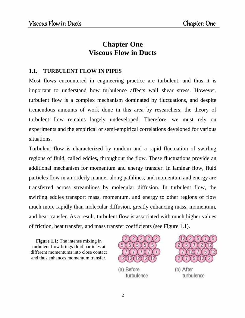
Turbulent flow is characterized by random and a rapid fluctuation of swirling

regions of fluid, called eddies, throughout the flow. These fluctuations provide an

additional mechanism for momentum and energy transfer. In laminar flow, fluid

particles flow in an orderly manner along pathlines, and momentum and energy are

transferred across streamlines by molecular diffusion. In turbulent flow, the

swirling eddies transport mass, momentum, and energy to other regions of flow

much more rapidly than molecular diffusion, greatly enhancing mass, momentum,

and heat transfer. As a result, turbulent flow is associated with much higher values

of friction, heat transfer, and mass transfer coefficients (see Figure 1.1).

Figure 1.1: The intense mixing in

turbulent flow brings fluid particles at

different momentums into close contact

and thus enhances momentum transfer.


3

Even when the average flow is steady, the eddy motion in turbulent flow causes

significant fluctuations in the values of velocity, temperature, pressure, and even

density (in compressible flow). Figure 1.2 shows the variation of the instantaneous

velocity component u with time at a specified location, as can be measured with a

hot-wire anemometer probe or other sensitive device. We observe that the

instantaneous values of the velocity fluctuate about an average value, which

suggests that the velocity can be expressed as the sum of an average value and a

fluctuating component ,

…….1.1

1.2. Turbulent Shear Stress

It is convenient to think of the turbulent shear stress as consisting of two parts: the

laminar component, which accounts for the friction between layers in the flow

direction (expressed as

), and the turbulent component, which

accounts for the friction between the fluctuating fluid particles and the fluid body

Figure 1.2: Fluctuations of the velocity component u with time at a specified location in

turbulent flow.


4

(denoted as ) and is related to the fluctuation components of velocity). Then

the total shear stress in turbulent flow can be expressed as

……1.2

The typical average velocity profile and relative magnitudes of laminar and

turbulent components of shear stress for turbulent flow in a pipe are given in

Figure 3.1.

In many of the simpler turbulence models, turbulent shear stress is expressed in an

analogous manner as suggested by the French mathematician Joseph Boussinesq

(1842–1929) in 1877 as

or

……1.3

where μt is the eddy viscosity or turbulent viscosity, which accounts for momentum

transport by turbulent eddies. Then the total shear stress can be expressed

conveniently as

……1.4

……1.5

where

⁄ is the kinematic eddy viscosity or kinematic turbulent viscosity

(also called the eddy diffusivity of momentum). The concept of eddy viscosity is

Figure 1.3: The velocity profile and the variation of shear stress with radial distance for

turbulent flow in a pipe.


5

very appealing, but it is of no practical use unless its value can be determined. In

other words, eddy viscosity must be modeled as a function of the average flow

variables; we call this eddy viscosity closure. For example, in the early 1900s, the

German engineer L. Prandtl introduced the concept of mixing length (lm), which is

related to the average size of the eddies that are primarily responsible for mixing,

and expressed the turbulent shear stress as

(

) ………1.6

1.3. Turbulent Velocity Profile

Unlike laminar flow, the expressions for the velocity profile in a turbulent flow are

based on both analysis and measurements, and thus they are semi-empirical in

nature with constants determined from experimental data. Consider fully-

developed turbulent flow in a pipe, and let u denote the time-averaged velocity in

the axial direction.

Typical velocity profiles for fully developed laminar and turbulent flows are given

in Figure 1.4. Note that the velocity profile is parabolic in laminar flow but is much

fuller in turbulent flow, with a sharp drop near the pipe wall. Turbulent flow along

a wall can be considered to consist of four regions, characterized by the distance

from the wall. The very thin layer next to the wall where viscous effects are

dominant is the viscous (or laminar or linear or wall) sublayer. The velocity

profile in this layer is very nearly linear, and the flow is streamlined. Next to the

viscous sublayer is the buffer layer, in which turbulent effects are becoming

significant, but the flow is still dominated by viscous effects. Above the buffer

layer is the overlap (or transition) layer, also called the inertial sublayer, in which

the turbulent effects are much more significant, but still not dominant. Above that


6

is the outer (or turbulent) layer in the remaining part of the flow in which

turbulent effects dominate over molecular diffusion (viscous) effects.

Then the velocity gradient in the viscous sublayer remains nearly constant at

du/dy= u/y, and the wall shear stress can be expressed as

…..1.7

where y is the distance from the wall (note that y= R - r for a circular pipe). The

quantity τw/ρ is frequently encountered in the analysis of turbulent velocity

profiles. The square root of τw/ρ has the dimensions of velocity, and thus it is

convenient to view it as a fictitious velocity called the friction velocity expressed

as √

⁄ . Substituting this into Eq. 1.7, the velocity profile in the viscous

sublayer can be expressed in dimensionless form as

Viscous sublayer:

Figure 1.4: The velocity profile in fully developed pipe flow is parabolic in laminar

flow, but much fuller in turbulent flow.


7

This equation is known as the law of the wall, and it is found to satisfactorily

correlate with experimental data for smooth surfaces for 0 ≤

≤5. Therefore, the

thickness of the viscous sublayer is roughly

Thickness of viscous sublayer:

where uϭ is the flow velocity at the edge of the viscous sublayer, which is closely

related to the average velocity in a pipe. The quantity

has dimensions of length

and is called the viscous length; it is used to nondimensionalize the distance y from

the surface. In boundary layer analysis, it is convenient to work with

nondimensionalized distance and nondimensionalized velocity defined as

Nondimensionalized variables:

Note that the friction velocity u* is used to nondimensionalize both y and u, and y+

resembles the Reynolds number expression.

Dimensional analysis indicates and the experiments confirm that the velocity in the

overlap layer is proportional to the logarithm of distance, and the velocity profile

can be expressed as

The logarithmic law: ……1.8

where k and B are constants whose values are determined experimentally to be

about 0.40 and 5.0, respectively. Equation 1.8 is known as the logarithmic law.

Substituting the values of the constants, the velocity profile is determined to be

Overlap layer:


8

A good approximation for the outer turbulent layer of pipe flow can be obtained by

evaluating the constant B in Eq. 1.8 from the requirement that maximum velocity

in a pipe occurs at the centerline where r= 0. Solving for B from Eq. 1.8 by setting

y = R & r = R and u = umax, and substituting it back into Eq. 1.8 together with k =

0.4 gives

Outer turbulent layer:

The deviation of velocity from the centerline value umax - u is called the velocity

defect, and the above equation is called the velocity defect law.

1.4. The Moody Chart

The friction factor in fully developed turbulent pipe flow depends on the Reynolds

number and the relative roughness (ε/D), which is the ratio of the mean height of

roughness of the pipe, to the pipe diameter. The functional form of this dependence

cannot be obtained from a theoretical analysis, and all available results are

obtained from painstaking experiments using artificially roughened surfaces

(usually by gluing sand grains of a known size on the inner surfaces of the pipes).

Most such experiments were conducted by Prandtl’s student J. Nikuradse in 1933,

followed by the works of others. The friction factor was calculated from the

measurements of the flow rate and the pressure drop.

The experimental results obtained are presented in tabular, graphical, and

functional forms obtained by curve-fitting experimental data. In 1939, Cyril F.

Colebrook (1910–1997) combined the available data for transition and turbulent

flow in smooth as well as rough pipes into the following implicit relation known as

the Colebrook equation:

Turbulent flow: …..1.9


9

We note that the logarithm in Eq. 1.9 is a base 10 rather than a natural logarithm.

In 1942, the American engineer Hunter Rouse (1906–1996) verified Colebrook’s

equation and produced a graphical plot of f as a function of Re and the product

√ . He also presented the laminar flow relation and a table of commercial pipe

roughness. Two years later, Lewis F. Moody (1880–1953) redrew Rouse’s diagram

into the form commonly used today. The now famous Moody chart is given in the

appendix as Figure 1.5. It presents the Darcy friction factor for pipe flow as a

function of the Reynolds number and ε/D over a wide range. It is probably one of

the most widely accepted and used charts in engineering. Although it is developed

for circular pipes, it can also be used for noncircular pipes by replacing the

diameter by the hydraulic diameter. An approximate explicit relation for f was

given by S. E. Haaland in 1983 as

…….. 1.10

The results obtained from this relation are within 2% of those obtained from the

Colebrook equation. Equivalent roughness values for some commercial pipes are

given in Table 1.1 as well as on the Moody chart.

Table 1.1: Equivalent roughness values

for new commercial pipes.


10

We make the following observations from the Moody chart:

For laminar flow, the friction factor decreases with increasing Reynolds

number, and it is independent of surface roughness.

The friction factor is a minimum for a smooth pipe (but still not zero

because of the no-slip condition) and increases with roughness. The

Colebrook equation in this case (ε = 0) reduces to the Prandtl equation

expressed as

The transition region from the laminar to turbulent regime (2300 < Re <

4000) is indicated by the shaded area in the Moody chart. The flow in this

region may be laminar or turbulent, depending on flow disturbances, or it

may alternate between laminar and turbulent, and thus the friction factor

may also alternate between the values for laminar and turbulent flow. The

data in this range are the least reliable. At small relative roughnesses, the

friction factor increases in the transition region and approaches the value for

smooth pipes.

At very large Reynolds numbers (to the right of the dashed line on the chart)

the friction factor curves corresponding to specified relative roughness

curves are nearly horizontal, and thus the friction factors are independent of

the Reynolds number. The flow in that region is called fully rough turbulent

flow or just fully rough flow because the thickness of the viscous sublayer

decreases with increasing Reynolds number, and it becomes so thin that it is

negligibly small compared to the surface roughness height. The viscous

effects in this case are produced in the main flow primarily by the protruding

roughness elements, and the contribution of the laminar sublayer is

negligible. The Colebrook equation in the fully rough zone (Re → ∞)

reduces to the von Kármán equation expressed as which is explicit in f.


11

Figure 1.5: The Moody chart for the friction factor for fully developed flow.

Figure 1.6: At very large Reynolds numbers, the friction factor curves on the Moody chart are

nearly horizontal, and thus the friction factors are independent of the Reynolds number.


12

1.5. Types of Fluid Flow Problems

In the design and analysis of piping systems that involve the use of the Moody

chart (or the Colebrook equation), we usually encounter three types of problems

(the fluid and the roughness of the pipe are assumed to be specified in all cases).

1. Determining the pressure drop (or head loss) when the pipe length and

diameter are given for a specified flow rate (or velocity)

2. Determining the flow rate when the pipe length and diameter are given for a

specified pressure drop (or head loss)

3. Determining the pipe diameter when the pipe length and flow rate are given for

a specified pressure drop (or head loss)

Problems of the first type are straightforward and can be solved directly by using

the Moody chart. Problems of the second type and third type are commonly

encountered in engineering design (in the selection of pipe diameter, for example,

that minimizes the sum of the construction and pumping costs), but the use of the

Moody chart with such problems requires an iterative approach unless an equation

solver is used.

In problems of the second type, the diameter is given but the flow rate is unknown.

A good guess for the friction factor in that case is obtained from the completely

turbulent flow region for the given roughness. This is true for large Reynolds

numbers, which is often the case in practice. Once the flow rate is obtained, the

friction factor can be corrected using the Moody chart or the Colebrook equation,

and the process is repeated until the solution converges. (Typically only a few

iterations are required for convergence to three or four digits of precision.)

In problems of the third type, the diameter is not known and thus the Reynolds

number and the relative roughness cannot be calculated. Therefore, we start

calculations by assuming a pipe diameter. The pressure drop calculated for the

assumed diameter is then compared to the specified pressure drop, and calculations

are repeated with another pipe diameter in an iterative fashion until convergence.


13

To avoid tedious iterations in head loss, flow rate, and diameter calculations,

Swamee and Jain proposed the following explicit relations in 1976 that are

accurate to within 2% of the Moody chart:

Examples:

Example 1:

Water (ρ= 62.36 lbm/ft3 and μ= 7.536×10

-4 lbm/ft·s) is flowing steadily in a 2 in

diameter horizontal pipe made of stainless steel at a rate of 0.2 ft3/s (see Figure

below). Determine the pressure drop, the head loss, and the required pumping

power input for flow over a 200 ft long section of the pipe.

Solution: We recognize this as a problem of

the first type, since flow rate, pipe length, and

pipe diameter are known. First we calculate

the average velocity and the Reynolds number

to determine the flow regime:

which is greater than 4000. Therefore, the flow is turbulent. The relative roughness

of the pipe is calculated using Table1.1.


14

The friction factor corresponding to this relative roughness and the Reynolds

number can simply be determined from the Moody chart. To avoid any reading

error, we determine f from the Colebrook equation:

Using an equation solver or an iterative scheme, the friction factor is determined to

be f = 0.0174. Then the pressure drop (which is equivalent to pressure loss in this

case), head loss, and the required power input become

Example 2:

Heated air at 35°C is to be transported in a 150 m long circular plastic duct at a rate

of 0.35 m3/s (see Figure below). If the head loss in the pipe is not to exceed 20 m,

determine the minimum diameter of the duct.

Solution:

The density, dynamic viscosity and kinematic viscosity of air at 35°C are ρ = 1.145

kg/m3, μ= 1.895×10

-5 kg/m·s, and = 1.655×10

-5 m

2/s.

the friction factor, and the head loss

relations can be expressed as (D is in m, V

is in m/s, and Re and f are dimensionless)


15

The roughness is approximately zero for a plastic pipe (Table 1.1). Therefore, this

is a set of four equations in four unknowns, and solving them with an equation

solver such as EES gives

Therefore, the diameter of the duct should be more than 26.7 cm if the head loss is

not to exceed 20 m. Note that Re > 4000, and thus the turbulent flow assumption is

verified.

The diameter can also be determined directly from the third Swamee–Jain formula

to be

Example:

Liquid ammonia at -20°C is flowing through a 30 m long section of a 5 mm

diameter copper tube at a rate of 0.15 kg/s. Determine the pressure drop, the head

loss, and the pumping power required to overcome the frictional losses in the tube.

Solution:


16

The density and dynamic viscosity of liquid ammonia at -20°C are ρ= 665.1 kg/m3

and μ= 2.361×10-4

kg/m.s. The roughness of copper tubing is 1.5×10-6

m.

First we calculate the average velocity and the Reynolds number to determine the

flow regime:

which is greater than Re > 4000. Therefore, the flow is turbulent. The relative

roughness of the pipe is

The friction factor can be determined from the Moody chart, but to avoid the

reading error, we determine it from the Colebrook equation using an equation

solver (or an iterative scheme),

It gives f = 0.01819. Then the pressure drop, the head loss, and the useful pumping

power required become

Fluid Mechanics II (ME 2305)

Documents

Transcript of Fluid Mechanics II (ME 2305)