Fluid Mechanics: Fundamentals and Applications€¦ · Fluid Mechanics: Fundamentals and...
103
Chapter 9 Differential Analysis of Fluid Flow 9-1 PROPRIETARY MATERIAL . © 2014 by McGraw-Hill Education. This is proprietary material solely for authorized instructor use. Not authorized for sale or distribution in any manner. This document may not be copied, scanned, duplicated, forwarded, distributed, or posted on a website, in whole or part. Solutions Manual for Fluid Mechanics: Fundamentals and Applications Third Edition Yunus A. Çengel & John M. Cimbala McGraw-Hill, 2013 Chapter 9 DIFFERENTIAL ANALYSIS OF FLUID FLOW PROPRIETARY AND CONFIDENTIAL This Manual is the proprietary property of The McGraw-Hill Companies, Inc. (“McGraw-Hill”) and protected by copyright and other state and federal laws. By opening and using this Manual the user agrees to the following restrictions, and if the recipient does not agree to these restrictions, the Manual should be promptly returned unopened to McGraw-Hill: This Manual is being provided only to authorized professors and instructors for use in preparing for the classes using the affiliated textbook. No other use or distribution of this Manual is permitted. This Manual may not be sold and may not be distributed to or used by any student or other third party. No part of this Manual may be reproduced, displayed or distributed in any form or by any means, electronic or otherwise, without the prior written permission of McGraw-Hill.
Transcript of Fluid Mechanics: Fundamentals and Applications€¦ · Fluid Mechanics: Fundamentals and...

Chapter 9 Differential Analysis of Fluid Flow
9-1 PROPRIETARY MATERIAL. © 2014 by McGraw-Hill Education. This is proprietary material solely for authorized instructor use. Not authorized for sale or distribution in any manner. This document may not be copied, scanned, duplicated, forwarded, distributed, or posted on a website, in whole or part.
Solutions Manual for
Fluid Mechanics: Fundamentals and Applications
Third Edition
Yunus A. Çengel & John M. Cimbala
McGraw-Hill, 2013
Chapter 9
DIFFERENTIAL ANALYSIS OF FLUID FLOW
PROPRIETARY AND CONFIDENTIAL This Manual is the proprietary property of The McGraw-Hill Companies, Inc. (“McGraw-Hill”) and protected by copyright and other state and federal laws. By opening and using this Manual the user agrees to the following restrictions, and if the recipient does not agree to these restrictions, the Manual should be promptly returned unopened to McGraw-Hill: This Manual is being provided only to authorized professors and instructors for use in preparing for the classes using the affiliated textbook. No other use or distribution of this Manual is permitted. This Manual may not be sold and may not be distributed to or used by any student or other third party. No part of this Manual may be reproduced, displayed or distributed in any form or by any means, electronic or otherwise, without the prior written permission of McGraw-Hill.

Chapter 9 Differential Analysis of Fluid Flow
9-2 PROPRIETARY MATERIAL. © 2014 by McGraw-Hill Education. This is proprietary material solely for authorized instructor use. Not authorized for sale or distribution in any manner. This document may not be copied, scanned, duplicated, forwarded, distributed, or posted on a website, in whole or part.
General and Mathematical Background Problems 9-1C Solution We are to express the divergence theorem in words.
Analysis For vector G
, the volume integral of the divergence of G
over volume V is equal to the surface
integral of the normal component of G
taken over the surface A that encloses the volume. Discussion The divergence theorem is also called Gauss’s theorem.
9-2C Solution We are to explain the fundamental differences between a flow domain and a control volume.
Analysis A control volume is used in an integral, control volume solution. It is a volume over which all mass flow rates, forces, etc. are specified over the entire control surface of the control volume. In a control volume analysis we do not know or care about details inside the control volume. Rather, we solve for gross features of the flow such as net force acting on a body. A flow domain, on the other hand, is also a volume, but is used in a differential analysis. Differential equations of motion are solved everywhere inside the flow domain, and we are interested in all the details inside the flow domain. Discussion Note that we also need to specify what is happening at the boundaries of a flow domain – these are called boundary conditions.
9-3C Solution We are to explain what we mean by coupled differential equations.
Analysis A set of coupled differential equations simply means that the equations are dependent on each other and must be solved together rather than separately. For example, the equations of motion for fluid flow involve velocity variables in both the conservation of mass equation and the momentum equation. To solve for these variables, we must solve the coupled set of differential equations together. Discussion In some very simple fluid flow problems, the equations become uncoupled, and are easier to solve.
9-4C Solution We are to discuss the number of unknowns and the equations needed to solve for those unknowns for a three-dimensional, unsteady, incompressible flow field. Analysis There are four unknowns (velocity components u, v, w, and pressure P) and thus we need to solve four equations:
one from conservation of mass which is a scalar equation three from Newton’s second law which is a vector equation
Discussion These equations are also coupled in general.

Chapter 9 Differential Analysis of Fluid Flow
9-3 PROPRIETARY MATERIAL. © 2014 by McGraw-Hill Education. This is proprietary material solely for authorized instructor use. Not authorized for sale or distribution in any manner. This document may not be copied, scanned, duplicated, forwarded, distributed, or posted on a website, in whole or part.
9-5C Solution We are to discuss the number of unknowns and the equations needed to solve for those unknowns for a two-dimensional, unsteady, compressible flow field with significant variations in both temperature and density.
Analysis There are five unknowns (velocity components u and v, and , T, and P) and thus we need to solve five equations:
one from conservation of mass which is a scalar equation two from Newton’s second law which is a vector equation one from the energy equation which is a scalar equation one from an equation of state (e.g., ideal gas law) which is a scalar equation
Discussion These equations are also coupled in general.
9-6C Solution We are to discuss the number of unknowns and the equations needed to solve for those unknowns for a two-dimensional, unsteady, incompressible flow field. Analysis There are three unknowns (velocity components u, and v, and pressure P) and thus we need to solve three equations:
one from conservation of mass which is a scalar equation two from Newton’s second law which is a vector equation
Discussion These equations are also coupled in general.
9-7 Solution We are to transform a position from Cartesian to cylindrical coordinates. Analysis We use the coordinate transformations provided in this chapter,
m 4.47214m) (4m) (2 2222 yxr (1)
and
radians 10715.143495.63m 2
m 4tantan 11
x
y (2)
Coordinate z remains unchanged. Thus, to three significant digits,
Position in cylindrical coordinates: )(),,( m 1 radians, 1.11 m, 4.47 zrx
(3)
Discussion Notice that the units of are radians – a dimensionless unit.

Chapter 9 Differential Analysis of Fluid Flow
9-4 PROPRIETARY MATERIAL. © 2014 by McGraw-Hill Education. This is proprietary material solely for authorized instructor use. Not authorized for sale or distribution in any manner. This document may not be copied, scanned, duplicated, forwarded, distributed, or posted on a website, in whole or part.
9-8 Solution We are to transform a position from cylindrical to Cartesian coordinates. Analysis We use the coordinate transformations provided in this chapter,
ocos 5 m cos / 3 radians 5 m cos 60 2.5 mx r (1)
and
osin 5 m sin / 3 radians 5 m sin 60 4.33013 my r (2)
Coordinate z remains unchanged. Thus, to three significant digits,
Position in cylindrical coordinates: , ,x x y z 2.50 m, 4.33 m, 1.27 m
(3)
Discussion You can verify your answer by using the reverse equations, as in the previous problem.
9-9 Solution We are to calculate a truncated Taylor series expansion for a given function and compare our result with the exact value. Analysis The algebra here is simple since d(ex)/dx = ex. The Taylor series expansion is
Taylor series expansion: 0 0 0 02 30
1 1( ) ...
2 3 2x x x xf x dx e e dx e dx e dx
(1)
We plug x0 = 0 and dx = –0.1 into Eq. 1,
Truncated Taylor series expansion:
2 31 1( 0.1) 1 1 ( 0.1) 1 ( 0.1) 1 ( 0.1) 0.9048333...
2 6f (2)
We compare Eq. 2 with the exact value,
Exact value: 0.1( 0.1) 0.904837418...f e (3)
Comparing Eqs. 2 and 3 we see that our approximation is good to four or five significant digits. Discussion The smaller the value of dx, the better the approximation. You can easily convince yourself of this by trying dx = 0.01 instead.
9-10 Solution We are to calculate the divergence of a given vector.
Analysis The divergence of G
is the dot product of the del operator i j kx y z
with G
, which gives
Divergence of G
: 2 212 2 0 2
2G i j k xzi x j z k z z
x y z
0
It turns out that for this special case, the divergence of G
is zero.
Discussion If G
were a velocity vector, this would mean that the flow field is incompressible.

Chapter 9 Differential Analysis of Fluid Flow
9-5 PROPRIETARY MATERIAL. © 2014 by McGraw-Hill Education. This is proprietary material solely for authorized instructor use. Not authorized for sale or distribution in any manner. This document may not be copied, scanned, duplicated, forwarded, distributed, or posted on a website, in whole or part.
9-11 Solution We are to expand the given equation in Cartesian coordinates and verify it.
Analysis In Cartesian coordinates the del operator is i j kx y z
and we let x y zF F i F j F k
and
x y zG G i G j G k
. The left hand side of the equation is thus
x x x y x z
y x y y y z
z x z y z z
x x y x z x
x y y y z y
x z y z z z
F G F G F G
FG F G F G F Gx y z
F G F G F G
F G F G F G ix y z
F G F G F G jx y z
F G F G F Gx y z
k
(1)
We use the product rule on each term in Eq. 1 and rearrange to get
Left hand side:
yx zx x y z x
yx zy x y z y
yx zz x y z
FF FFG G F F F G i
x y z x y z
FF FG F F F G j
x y z x y z
FF FG F F F
x y z x y z
zG k
(2)
We recognize that yx zFF F
Fx y z
and x y zF F F F
x y z
. Eq. 2 then becomes
Left hand side:
x x y y
z z
FG G F F G i G F F G j
G F F G k
(3)
After rearrangement, Eq. 3 becomes
Left hand side:
x y z x y zFG G i G j G k F F G i G j G k
(4)
Finally, recognizing vector G
twice in Eq. 4, we see that the left hand side of the given equation is identical to the right hand side, and the given equation is verified.
Discussion It may seem surprising, but FG GF
.

Chapter 9 Differential Analysis of Fluid Flow
9-6 PROPRIETARY MATERIAL. © 2014 by McGraw-Hill Education. This is proprietary material solely for authorized instructor use. Not authorized for sale or distribution in any manner. This document may not be copied, scanned, duplicated, forwarded, distributed, or posted on a website, in whole or part.
9-12 Solution We are to prove the equation.
Analysis We let F V
and G V
. Using Eq. 1 of the previous problem, we have
VV V V V V
(1)
However, since the density is not operated on in the second term of Eq. 1, it can be brought outside of the parenthesis, even though it is not a constant in general. Equation 1 can thus be written as
VV V V V V
(2)
Discussion Equation 2 was used in this chapter in the derivation of the alternative form of Cauchy’s equation.
9-13 Solution We are to transform cylindrical velocity components to Cartesian velocity components. Analysis We apply trigonometry, recognizing that the angle between u and ur is , and the angle between v and u is also ,
x component of velocity: cos sinru u u (1)
Similarly,
y component of velocity: sin cosrv u u (2)
The transformation of the z component is trivial,
z component of velocity: zw u (3)
Discussion These transformations come in handy.
9-14 Solution We are to transform Cartesian velocity components to cylindrical velocity components. Analysis We apply trigonometry, recognizing that the angle between u and ur is , and the angle between v and u is also ,
ur component of velocity: cos sinru u v (1)
Similarly,
u component of velocity:: sin cosu u v (2)
The transformation of the z component is trivial,
z component of velocity: zu w (3)
Discussion You can also obtain Eqs. 1 and 2 by solving Eqs. 1 and 2 of the previous problem simultaneously.

Chapter 9 Differential Analysis of Fluid Flow
9-7 PROPRIETARY MATERIAL. © 2014 by McGraw-Hill Education. This is proprietary material solely for authorized instructor use. Not authorized for sale or distribution in any manner. This document may not be copied, scanned, duplicated, forwarded, distributed, or posted on a website, in whole or part.
9-15 Solution We are to transform a given set of Cartesian coordinates and velocity components into cylindrical coordinates and velocity components.
Analysis First we apply the coordinate transformations given in this chapter,
2 22 2 0.40 m 0.20 m 0.4472 mr x y (1)
1 1 o0.20 mtan tan 26.565 0.4636 radians
0.40 m
y
x
(2)
Next we apply the results of the previous problem,
m 0.40 m m 0.20 m m
cos sin 10.3 5.6 6.708s 0.4472 m s 0.4472 m sru u v (3)
m 0.20 m m 0.40 m m
sin cos 10.3 5.6 9.615s 0.4472 m s 0.4472 m s
u u v (4)
Note that we have used the fact that x = rcos and y = rsin for convenience in Eqs. 3 and 4. Our final results are summarized to three significant digits:
Results: m m
0.447 m, 0.464 radians, 6.71 , 9.62s srr u u (5)
We verify our result by calculating the square of the speed in both coordinate systems. In Cartesian coordinates,
2 2 2
2 2 22
m m m10.3 5.6 137.5
s s sV u v
(6)
In cylindrical coordinates,
2 2 2
2 2 22
m m m6.708 9.615 137.5
s s srV u u
(7)
Discussion Such checks of our algebra are always wise.
9-16 Solution We are to transform a given set of Cartesian velocity components into cylindrical velocity components, and identify the flow.
Assumptions 1 The flow is steady. 2 The flow is incompressible. 3 The flow is two-dimensional in the x-y or r- plane.
Analysis We recognize that 2 2 2r x y . We also know that y = rsin and x = rcos. Using the results of Problem 9-
14, the cylindrical velocity components are
ur component of velocity: 2 2
sin cos sin coscos sin 0r
Cr Cru u v
r r
(1)
u component of velocity:: 2 2
2 2
sin cossin cos
Cr Cr Cu u v
rr r
(2)
where we have also used the fact that cos2 + sin2 = 1. We recognize the velocity components of Eqs. 1 and 2 as those of a line vortex.
Discussion The negative sign in Eq. 2 indicates that this vortex is in the clockwise direction.

Chapter 9 Differential Analysis of Fluid Flow
9-8 PROPRIETARY MATERIAL. © 2014 by McGraw-Hill Education. This is proprietary material solely for authorized instructor use. Not authorized for sale or distribution in any manner. This document may not be copied, scanned, duplicated, forwarded, distributed, or posted on a website, in whole or part.
9-17 Solution We are to transform a given set of cylindrical velocity components into Cartesian velocity components. Analysis We apply the coordinate transformations given in this chapter, along with the results of Problem 9-16,
x component of velocity: cos sin2 2r
m x yu u u
r r r r
(1)
We recognize that 2 2 2r x y . Thus, Eq. 1 becomes
x component of velocity:
2 2
1
2u mx y
x y
(2)
Similarly,
y component of velocity: sin cos2 2r
m y xv u u
r r r r
(3)
Again recognizing that 2 2 2r x y , Eq. 3 becomes
y component of velocity:
2 2
1
2v my x
x y
(4)
We verify our result by calculating the square of the speed in both coordinate systems. In Cartesian coordinates,
2 2 2 2 2 2 2 2 2 2 22 22 2 2 2 2 2
1 12 2
4 4V u v m x mx y y m y my x x
x y x y
(5)
Two of the terms in Eq. 5 cancel, and we combine the others. After simplification,
Magnitude of velocity squared: 2 2 2 2 2
2 2 2
1
4V u v m
x y
(6)
We calculate V2 from the components given in cylindrical coordinates as well,
Magnitude of velocity squared: 2 2 2 2
2 2 22 2 2 2 2 24 4 4r
m mV u u
r r r
(7)
Finally, since 2 2 2r x y , Eqs. 6 and 7 are the same, and the results are verified.
Discussion Such checks of our algebra are always wise.

Chapter 9 Differential Analysis of Fluid Flow
9-9 PROPRIETARY MATERIAL. © 2014 by McGraw-Hill Education. This is proprietary material solely for authorized instructor use. Not authorized for sale or distribution in any manner. This document may not be copied, scanned, duplicated, forwarded, distributed, or posted on a website, in whole or part.
9-18E Solution We are to transform a given set of Cartesian coordinates and velocity components into cylindrical coordinates and velocity components.
Analysis First we apply the coordinate transformations given in this chapter,
o 1 ftcos 5.20 in cos 30.0 0.3753 ft
12 inx r
(1)
and
o 1 ftsin 5.20 in sin 30.0 0.2167 ft
12 iny r
(2)
Next we apply the results of a previous problem, ft/s 5460.0)(30.0sinft/s) 66.4()cos(30.0ft/s) 06.2(sincos uuu r (3)
and ft/s 066.5)(30.0cosft/s) 66.4()(30.0sinft/s) 06.2(cossin uuv r (4)
Our final results are summarized to three significant digits: Results: ft/s 5.07ft/s 0.546ft 0.217ft 0.373 vuyx , , , (5)
We verify our result by calculating the square of the speed in both coordinate systems. In Cartesian coordinates,
22 /sft 25.96 22222 ft/s) (5.066ft/s) 0.5460(vuV (6)
In cylindrical coordinates,
22 /sft 25.96 22222 ft/s) (4.66ft/s) (2.06uuV r (7)
Discussion Such checks of our algebra are always wise.

Chapter 9 Differential Analysis of Fluid Flow
9-10 PROPRIETARY MATERIAL. © 2014 by McGraw-Hill Education. This is proprietary material solely for authorized instructor use. Not authorized for sale or distribution in any manner. This document may not be copied, scanned, duplicated, forwarded, distributed, or posted on a website, in whole or part.
9-19 Solution We are to perform both integrals of the divergence theorem for a given vector and volume, and verify that they are equal.
Analysis We do the volume integral first:
Volume integral: 1 1 1 1 1 1
0 0 0 0 0 04 2
x y z x y zyx z
x y z x y z
GG GGd dzdydx z y y dzdydx
x y z
V
V
(1)
The term in parentheses in Eq. 1 reduces to (4z – y), and we integrate this over z first,
1 1 1 112
00 0 0 02 2
x y x yz
zx y x yGd z yz dydx y dydx
V
V
Then we integrate over y and then over x,
Volume integral: 12
1 1
0 00
32
2 2
yx x
x xy
yGd y dx dx
3
2VV
(2)
Next we calculate the surface integral of the divergence theorem. There are six faces of the cube, and unit vector n
points outward from each face. So, we split the area integral into six parts and sum them. E.g., the right-most face has n
= (1,0,0),
so G n
= 4xz on this face. The bottom face has n
= (0,–1,0), so G n
= y2 on this face. The surface integral is then
Surface integral:
1 1 1 1 1 1 2
0 0 0 0 0 01 0 1
Right face Left face Top face
1 1 2
0 0
4 4
y z y z z x
A y z y z z xx x y
z x
z x
G ndA xz dzdy xz dzdy y dxdz
y dxdz
1 1 1 1
0 0 0 00 1 0
Front face Back faceBottom face
x y x y
x y x yy z z
yz dydx yz dydx
(3)
The three integrals on the far right of Eq. 3 are obviously zero. The other three integrals can be obtained carefully,
12
1 1 1 1 1 11 12
000 0 0 0 0 00
12 2 1
2 2
yy z x y z xz x
xzA y z x y z xy
yG ndA z dy x dz dx dy dz dx
(4)
The last three integrals of Eq. 4 are trivial. The final result is
Surface integral: 1
2 12A
G ndA 3
2
(5)
Since Eq. 2 and Eq. 5 are equal, the divergence theorem works for this case.
Discussion The integration is simple in this example since each face is flat and normal to an axis. In the general case in which the surface is curved, integration is much more difficult, but the divergence theorem always works.
Chapter 9 Differential Analysis of Fluid Flow
9-11 PROPRIETARY MATERIAL. © 2014 by McGraw-Hill Education. This is proprietary material solely for authorized instructor use. Not authorized for sale or distribution in any manner. This document may not be copied, scanned, duplicated, forwarded, distributed, or posted on a website, in whole or part.
9-20 Solution We are to expand a dot product in Cartesian coordinates and verify it.
Analysis In Cartesian coordinates the del operator is i j kx y z
and we let x y zG G i G j G k
. The
left hand side of the equation is thus
Left hand side:
yx z
yx zx y z
fGfG fGfG
x y z
GG Gf f fG f G f G f
x x y y z z
(1)
The right hand side of the equation is
Right hand side:
yx zx y z
yx zx y z
G f f G
GG Gf f fG i G j G k i j k f
x y z x y z
GG Gf f fG G G f f f
x y z x y z
(2)
Equations 1 and 2 are the same, and the given equation is verified. Discussion The product rule given in this problem was used in this chapter in the derivation of the alternative form of the continuity equation.
Chapter 9 Differential Analysis of Fluid Flow
9-12 PROPRIETARY MATERIAL. © 2014 by McGraw-Hill Education. This is proprietary material solely for authorized instructor use. Not authorized for sale or distribution in any manner. This document may not be copied, scanned, duplicated, forwarded, distributed, or posted on a website, in whole or part.
Continuity Equation 9-21C Solution We are to explain why the derivation of the continuity via the divergence theorem is so much less involved than the derivation of the same equation by summation of mass flow rates through each face of an infinitesimal control volume. Analysis In the derivation using the divergence theorem, we begin with the control volume form of conservation of mass, and simply apply the divergence theorem. The control volume form was already derived in Chap. 5, so we begin the derivation in this chapter with an established conservation of mass equation. On the other hand, the alternative derivation is from “scratch” and therefore requires much more algebra. Discussion The bottom line is that the divergence theorem enables us to quickly convert the control volume form of the conservation law into the differential form.
9-22C Solution We are to discuss the material derivative of density for the case of compressible and incompressible flow. Analysis If the flow field is compressible, we expect that as a fluid particle (a material element) moves around in the flow, its density changes. Thus the material derivative of density (the rate of change of density following a fluid particle) is non-zero for compressible flow. However, if the flow field is incompressible, the density remains constant. As a fluid particle moves around in the flow, the material derivative of density must be zero for incompressible flow (no change in density following the fluid particle). Discussion The material derivative of any property is the rate of change of that property following a fluid particle.

Chapter 9 Differential Analysis of Fluid Flow
9-13 PROPRIETARY MATERIAL. © 2014 by McGraw-Hill Education. This is proprietary material solely for authorized instructor use. Not authorized for sale or distribution in any manner. This document may not be copied, scanned, duplicated, forwarded, distributed, or posted on a website, in whole or part.
9-23 Solution We are to repeat Example 9-1, but without using continuity.
Assumptions 1 Density varies with time, but not space; in other words, the density is uniform throughout the cylinder at any given time, but changes with time. 2 No mass escapes from the cylinder during the compression.
Analysis The mass inside the cylinder is constant, but the volume decreases linearly as the piston moves up. At t = 0 when L = LBottom the initial volume of the cylinder is V(0) = LBottomA, where A is the cross-sectional area of the cylinder. At t = 0 the density is = (0) = m/V(0), and thus
Mass in the cylinder: Bottom0 0 0m V L A (1)
Mass m (Eq. 1) is a constant since no mass escapes during the compression. At some later time t, Bottom PL L V t and the
volume is thus
Cylinder volume at time t: Bottom PL V t A V (2)
The density at time t is
Density at time t:
Bottom
Bottom P
0 L Am
L V t A
V (3)
where we have plugged in Eq. 1 for m and Eq. 2 for V. Equation 3 reduces to
Bottom
Bottom P
(0)L
L V t
(4)
or, using the nondimensional variables of Example 9-1,
Nondimensional result: P
Bottom
1 1 or *
(0) 1 *1V t t
L
(5)
which is identical to Eq. 5 of Example 9-1.
Discussion We see by this exercise that the continuity equation is indeed an equation of conservation of mass.
9-24 Solution We are to expand the continuity equation in Cartesian coordinates.
Analysis We expand the second term by taking the dot product of the del operator i j kx y z
with
V u i v j w k
, giving
Compressible continuity equation in Cartesian coordinates:
0u v w
t x y z
(1)
We can further expand Eq. 1 by using the product rule on the spatial derivatives, resulting in 7 terms,
Further expansion: 0u v w
u v wt x x y y z z
(2)
Discussion We can do a similar thing in cylindrical coordinates, but the algebra is somewhat more complicated.

Chapter 9 Differential Analysis of Fluid Flow
9-14 PROPRIETARY MATERIAL. © 2014 by McGraw-Hill Education. This is proprietary material solely for authorized instructor use. Not authorized for sale or distribution in any manner. This document may not be copied, scanned, duplicated, forwarded, distributed, or posted on a website, in whole or part.
9-25 Solution We are to write the given equation as a word equation and discuss it. Analysis Here is a word equation: “The time rate of change of volume of a fluid particle per unit volume is equal to the divergence of the velocity field.” As a fluid particle moves around in a compressible flow, it can distort, rotate, and get larger or smaller. Thus the volume of the fluid element can change with time; this is represented by the left hand side of the equation. The right hand side is identically zero for an incompressible flow, but it is not zero for a compressible flow. Thus we can think of the volumetric strain rate as a measure of compressibility of a fluid flow. Discussion Volumetric strain rate is a kinematic property as discussed in Chap. 4. Nevertheless, it is shown here to be related to the continuity equation (conservation of mass).
9-26 Solution We are to verify that a given flow field satisfies the continuity equation, and we are to discuss conservation of mass at the origin. Analysis The 2-D cylindrical velocity components (ur,u) for this flow field are
Cylindrical velocity components: 2 2r
mu u
r r
(1)
where m and are constants We plug Eq. 1 into the incompressible continuity equation in cylindrical coordinates,
Incompressible continuity:
1 1 1 20 or r z
mru u u
r r r z r r
0
1 2 r
r
0
zu
z
0
0
(2)
The first term is zero because it is the derivative of a constant. The second term is zero because r is not a function of . The third term is zero since this is a 2-D flow with uz = 0. Thus, we verify that the incompressible continuity equation is satisfied for the given velocity field. At the origin, both ur and u go to infinity. Conservation of mass is not affected by u, but the fact that ur is non-zero at the origin violates conservation of mass. We think of the flow along the z axis as a line sink toward which mass approaches from all directions in the plane and then disappears (like a black hole in two dimensions). Mass is not conserved at the origin. Discussion Singularities such as this are unphysical of course, but are nevertheless useful as approximations of real flows, as long as we stay away from the singularity itself.

Chapter 9 Differential Analysis of Fluid Flow
9-15 PROPRIETARY MATERIAL. © 2014 by McGraw-Hill Education. This is proprietary material solely for authorized instructor use. Not authorized for sale or distribution in any manner. This document may not be copied, scanned, duplicated, forwarded, distributed, or posted on a website, in whole or part.
9-27 Solution We are to verify that a given velocity field satisfies continuity. Assumptions 1 The flow is steady. 2 The flow is incompressible. 3 The flow is two-dimensional in the x-y plane. Analysis The velocity field of Problem 9-16 is
Cartesian velocity components: 2 2 2 2
Cy Cx
u vx y x y
(1)
We check continuity, staying in Cartesian coordinates,
3 32 2 2 22 2xCy x y yCx x y
u v w
x y z
0 since 2-D
0
So we see that the incompressible continuity equation is indeed satisfied. Discussion The fact that the flow field satisfies continuity does not guarantee that a corresponding pressure field exists that can satisfy the steady conservation of momentum equation. In this case, however, it does.
9-28 Solution We are to verify that a given velocity field is incompressible.
Assumptions 1 The flow is two-dimensional, implying no z component of velocity and no variation of u or v with z.
Analysis The components of velocity in the x and y directions respectively are
1.6 1.8 1.5 1.8u x v y
To check if the flow is incompressible, we see if the incompressible continuity equation is satisfied:
2.8 2.8
u v w
x y z
0 since 2-D
0 or 1.8 1.8 0
So we see that the incompressible continuity equation is indeed satisfied. Hence the flow field is incompressible.
Discussion The fact that the flow field satisfies continuity does not guarantee that a corresponding pressure field exists that can satisfy the steady conservation of momentum equation.

Chapter 9 Differential Analysis of Fluid Flow
9-16 PROPRIETARY MATERIAL. © 2014 by McGraw-Hill Education. This is proprietary material solely for authorized instructor use. Not authorized for sale or distribution in any manner. This document may not be copied, scanned, duplicated, forwarded, distributed, or posted on a website, in whole or part.
9-29 Solution For a given axial velocity component in an axisymmetric flow field, we are to generate the radial velocity component. Assumptions 1 The flow is steady. 2 The flow is incompressible. 3 The flow is axisymmetric implying that u = 0 and there is no variation in the direction. Analysis We use the incompressible continuity equation in cylindrical coordinates, simplified as follows for axisymmetric flow,
Incompressible axisymmetric continuity equation: 1
0r zru u
r r z
(1)
We rearrange Eq. 1,
,exit ,entrancer z z zru u u u
r rr z L
(2)
We integrate Eq. 2 with respect to r,
2
,exit ,entrance
2z z
r
u urru f z
L
(3)
Notice that since we performed a partial integration with respect to r, we add a function of the other variable z rather than simply a constant of integration. We divide all terms in Eq. 3 by r and recognize that the term with f(z) will go to infinity at the centerline of the nozzle (r = 0) unless f(z) = 0. We write our final expression for ur,
Radial velocity component: ,exit ,entrance
2z z
r
u uru
L
(4)
Discussion You should plug the given equation and Eq. 4 into Eq. 1 to verify that the result is correct. (It is.)
9-30 Solution We are to determine a relationship between constants a, b, c, and d that ensures incompressibility.
Assumptions 1 The flow is steady. 2 The flow is incompressible (under certain restraints to be determined).
Analysis We plug the given velocity components into the incompressible continuity equation,
Condition for incompressibility:
2 26ay cy
u v w
x y z
2 2
0
0 6 0ay cy
Thus to guarantee incompressibility, constants a and c must satisfy the following relationship:
Condition for incompressibility: 6a c (1)
Discussion If Eq. 1 were not satisfied, the given velocity field might still represent a valid flow field, but density would have to vary with location in the flow field – in other words the flow would be compressible.

Chapter 9 Differential Analysis of Fluid Flow
9-17 PROPRIETARY MATERIAL. © 2014 by McGraw-Hill Education. This is proprietary material solely for authorized instructor use. Not authorized for sale or distribution in any manner. This document may not be copied, scanned, duplicated, forwarded, distributed, or posted on a website, in whole or part.
9-31 Solution We are to determine a relationship between constants a, b, c, and d that ensures incompressibility. Assumptions 1 The flow is steady. 2 The flow is incompressible (under certain restraints to be determined). Analysis We plug the given velocity components into the incompressible continuity equation,
Condition for incompressibility: 2 2axy cxy
u v w
x y z
0
0 2 2 0axy cxy
Thus to guarantee incompressibility, constants a and c must satisfy the following relationship:
Condition for incompressibility: a c (1)
Discussion If Eq. 1 were not satisfied, the given velocity field might still represent a valid flow field, but density would have to vary with location in the flow field – in other words the flow would be compressible.
9-32 Solution We are to find the y component of velocity, v, using a given expression for u. Assumptions 1 The flow is steady. 2 The flow is incompressible. 3 The flow is two-dimensional in the x-y plane, implying that w = 0 and neither u nor v depend on z. Analysis Since the flow is steady and incompressible, we apply the incompressible continuity in Cartesian coordinates to the flow field, giving
Condition for incompressibility:
a
v u w
y x z
0
v
ay
Next we integrate with respect to y. Note that since the integration is a partial integration, we must add some arbitrary function of x instead of simply a constant of integration.
Solution: v ay f x
If the flow were three-dimensional, we would add a function of x and z instead. Discussion To satisfy the incompressible continuity equation, any function of x will work since there are no derivatives of v with respect to x in the continuity equation. Not all functions of x are necessarily physically possible, however, since the flow must also satisfy the steady conservation of momentum equation.

Chapter 9 Differential Analysis of Fluid Flow
9-18 PROPRIETARY MATERIAL. © 2014 by McGraw-Hill Education. This is proprietary material solely for authorized instructor use. Not authorized for sale or distribution in any manner. This document may not be copied, scanned, duplicated, forwarded, distributed, or posted on a website, in whole or part.
9-33 Solution We are to find the most general form of the tangential velocity component of a purely circular flow that does not violate conservation of mass. Assumptions 1 The flow is steady. 2 The flow is incompressible. 3 The flow is two-dimensional in the x-y or r- plane. Analysis We use cylindrical coordinates for convenience. We solve for u using the incompressible continuity equation,
1 rru
r r
0 for circular flow
1 zu u
r z
0 for 2-D flow
0 or 0u
(1)
We integrate Eq. 1 with respect to , adding a function of the other variable r rather than simply a constant of integration since this is a partial integration,
Result: u f r (2)
Discussion Any function of r in Eq. 2 will satisfy the continuity equation.
9-34 Solution We are to find the y component of velocity, v, using a given expression for u.
Assumptions 1 The flow is steady. 2 The flow is incompressible. 3 The flow is two-dimensional in the x-y plane, implying that w = 0 and neither u nor v depend on z. Analysis We plug the velocity components into the steady incompressible continuity equation,
Condition for incompressibility:
a
v u w
y x z
0
v
ay
Next we integrate with respect to y. Note that since the integration is a partial integration, we must add some arbitrary function of x instead of simply a constant of integration.
Solution: v ay f x
If the flow were three-dimensional, we would add a function of x and z instead. Discussion To satisfy the incompressible continuity equation, any function of x will work since there are no derivatives of v with respect to x in the continuity equation. Not all functions of x are necessarily physically possible, however, since the flow may not be able to satisfy the steady conservation of momentum equation.

Chapter 9 Differential Analysis of Fluid Flow
9-19 PROPRIETARY MATERIAL. © 2014 by McGraw-Hill Education. This is proprietary material solely for authorized instructor use. Not authorized for sale or distribution in any manner. This document may not be copied, scanned, duplicated, forwarded, distributed, or posted on a website, in whole or part.
9-35 Solution We are to find the y component of velocity, v, using a given expression for u.
Assumptions 1 The flow is steady. 2 The flow is incompressible. 3 The flow is two-dimensional in the x-y plane, implying that w = 0 and neither u nor v depend on z.
Analysis We plug the velocity components into the steady incompressible continuity equation,
Condition for incompressibility:
6 2ax by
v u w
y x z
0
6 2v
ax byy
Next we integrate with respect to y. Note that since the integration is a partial integration, we must add some arbitrary function of x instead of simply a constant of integration.
Solution: 26v axy by f x
If the flow were three-dimensional, we would add a function of x and z instead.
Discussion To satisfy the incompressible continuity equation, any function of x will work since there are no derivatives of v with respect to x in the continuity equation.
9-36 Solution We are to find the most general form of the radial velocity component of a purely radial flow that does not violate conservation of mass. Assumptions 1 The flow is steady. 2 The flow is incompressible. 3 The flow is two-dimensional in the x-y or r- plane. Analysis We use cylindrical coordinates for convenience. We solve for ur using the incompressible continuity equation,
1 1rru u
r r r
0 for radial flow
zu
z
0 for 2-D flow
0 or 0rru
r
(1)
We integrate Eq. 1 with respect to r, adding a function of the other variable rather than simply a constant of integration since this is a partial integration,
Result: or r r
fru f u
r
(2)
Discussion Any function of in Eq. 2 will satisfy the continuity equation.

Chapter 9 Differential Analysis of Fluid Flow
9-20 PROPRIETARY MATERIAL. © 2014 by McGraw-Hill Education. This is proprietary material solely for authorized instructor use. Not authorized for sale or distribution in any manner. This document may not be copied, scanned, duplicated, forwarded, distributed, or posted on a website, in whole or part.
9-37 Solution We are to find the z component of velocity using given expressions for u and v.
Assumptions 1 The flow is steady. 2 The flow is incompressible.
Analysis We apply the steady incompressible continuity equation to the given flow field,
Condition for incompressibility:
2
2
2
2
a bybz
w u v wa by bz
z x y z
Next we integrate with respect to z. Note that since the integration is a partial integration, we must add some arbitrary function of x and y instead of simply a constant of integration.
Solution: 3
2 ,3
bzw az byz f x y
Discussion To satisfy the incompressible continuity equation, any function of x and y will work since there are no derivatives of w with respect to x or y in the continuity equation.

Chapter 9 Differential Analysis of Fluid Flow
9-21 PROPRIETARY MATERIAL. © 2014 by McGraw-Hill Education. This is proprietary material solely for authorized instructor use. Not authorized for sale or distribution in any manner. This document may not be copied, scanned, duplicated, forwarded, distributed, or posted on a website, in whole or part.
9-38
Solution For given velocity component u and density , we are to predict velocity component v, plot an approximate shape of the duct, and predict its height at section (2).
Assumptions 1 The flow is steady and two-dimensional in the x-y plane, but compressible. 2 Friction on the walls is ignored. 3 Axial velocity u and density vary linearly with x. 4 The x axis is a line of top-bottom symmetry.
Properties The fluid is standard air. The speed of sound is about 340 m/s, so the flow is subsonic, but compressible.
Analysis (a) We write expressions for u and , forcing them to be linear in x,
2 11
m100 300 1s 100
2.0 m su u
u uu u C x C
x
(1)
3
2 11 4
kg1.2 0.85 kgm 0.175
2.0 m mC x C
x
(2)
where Cu and C are constants. We use the compressible form of the steady continuity equation, placing the unknown term v on the left hand side, and plugging in Eqs. 1 and 2,
1 1 uC x u C xv u
y x x
After some algebra,
1 1 2u u
vC u C C C x
y
(3)
We integrate Eq. 3 with respect to y,
1 1 2u uv C u C y C C xy f x (4)
Since this is a partial integration, we add an arbitrary function of x instead of simply a constant of integration. We now apply boundary conditions. Since the flow is symmetric about the x axis (y = 0), v must equal zero at y = 0 for any x. This is possible only if f(x) is identically zero. Applying f(x) = 0, dividing by to solve for v, and plugging in Eq. 2, Eq. 4 becomes
1 1 1 1
1
2 2u u u uC u C y C C xy C u C y C C xyv
C x
(5)
(b) For known values of u and v, we can plot streamlines between x = 0 and x = 2.0 m using the technique described in Chap. 4. Several streamlines are shown in Fig. 1. The streamline starting at x = 0, y = 0.8 m is the top wall of the duct.
(c) At section (2), the top streamline crosses y = 1.70 m at x = 2.0 m. Thus, the predicted height of the duct at section (2) is 1.70 m.
Discussion You can verify that the combination of Eqs. 1, 2, and 5 satisfies the steady compressible continuity equation. However, this alone does not guarantee that the density and velocity components will actually follow these equations if this diverging duct were to be built. The actual flow depends on the pressure rise between sections (1) and (2) – only one unique pressure rise can yield the desired flow deceleration. Temperature may also change considerably in this kind of compressible flow field.
0
0.5
1
1.5
2
0 0.5 1 1.5 2x
y Top wall
Symmetry line
FIGURE 1 Streamlines for a diverging duct.

Chapter 9 Differential Analysis of Fluid Flow
9-22 PROPRIETARY MATERIAL. © 2014 by McGraw-Hill Education. This is proprietary material solely for authorized instructor use. Not authorized for sale or distribution in any manner. This document may not be copied, scanned, duplicated, forwarded, distributed, or posted on a website, in whole or part.
Stream Function 9-39C Solution We are to discuss the significance of the difference in value of stream function from one streamline to another.
Analysis The difference in the value of from one streamline to another is equal to the volume flow rate per unit width between the two streamlines.
Discussion This fact about the stream function can be used to calculate the volume flow rate in certain applications.
9-40C Solution We are to discuss why the stream function is called a non-primitive variable in CFD lingo. Analysis The natural physical variables in a fluid flow problem are the velocity components and the pressure. [If the flow is compressible, density and temperature are also natural physical variables.] These variables can be considered “primitive” because we do not change them in any way – we simply solve for them directly. Stream function, on the other hand, is a contrived or derived variable. The stream function is not primitive in the sense that it is not one of the original physical variables in the problem. Discussion Vorticity is another example of a non-primitive variable. In fact, some 2-D CFD codes use stream function and vorticity as the variables – non-primitive variables.
9-41C Solution We are to discuss the restrictions on the stream function that cause it to exactly satisfy 2-D incompressible continuity, and why they are necessary.
Analysis Stream function must be a smooth function of x and y (or r and ). These restrictions are necessary so that the second derivatives of with respect to both variables are equal regardless of the order of differentiation. In other
words, if 2 2
x y y x
, then the 2-D incompressible continuity equation is satisfied exactly by the definition of .
Discussion If the stream function were not smooth, there would be sudden discontinuities in the velocity field as well – a physical impossibility that would violate conservation of mass.
9-42C Solution We are to discuss the significance of curves of constant stream function, and why the stream function is useful.
Analysis Curves of constant stream function represent streamlines of a flow. A stream function is useful because by drawing curves of constant , we can visualize the instantaneous velocity field. In addition, the change in the value of from one streamline to another is equal to the volume flow rate per unit width between the two streamlines.
Discussion Streamlines are an instantaneous flow description, as discussed in Chap. 4.

Chapter 9 Differential Analysis of Fluid Flow
9-23 PROPRIETARY MATERIAL. © 2014 by McGraw-Hill Education. This is proprietary material solely for authorized instructor use. Not authorized for sale or distribution in any manner. This document may not be copied, scanned, duplicated, forwarded, distributed, or posted on a website, in whole or part.
9-43 Solution For a given velocity field we are to generate an expression for , and we are to calculate the volume flow rate per unit width between two streamlines. Assumptions 1 The flow is steady. 2 The flow is incompressible. 3 The flow is two-dimensional in the x-y plane. Analysis We start by picking one of the two definitions of the stream function (it doesn’t matter which part we choose – the solution will be identical).
u Vy
(1)
Next we integrate Eq. 1 with respect to y, noting that this is a partial integration and we must add an arbitrary function of the other variable, x, rather than a simple constant of integration.
Vy g x (2)
Now we choose the other part of the definition of , differentiate Eq. 2, and rearrange as follows:
v g xx
(3)
where g(x) denotes dg/dx since g is a function of only one variable, x. We now have two expressions for velocity component v, the given equation and Eq. 3. We equate these and integrate with respect to x to find g(x),
0 0 v g x g x g x C (4)
Note that here we have added an arbitrary constant of integration C since g is a function of x only. Finally, plugging Eq. 4 into Eq. 2 yields the final expression for ,
Stream function: Vy C (5)
Constant C is arbitrary; it is common to set it to zero, although it can be set to any desired value. Here, = 0 along the streamline at y = 0, forcing C to equal zero by Eq. 5. For the streamline at y = 0.5 m,
Value of 2: 2
2
m m6.94 0.5 m 3.47
s s
(6)
The volume flow rate per unit width between streamlines 2 and 0 is equal to 2 – 0,
Volume flow rate per unit width: 2
2 0
m3.47 0
sW
2m3.47
s
V (7)
We verify our result by calculating the volume flow rate per unit width from first principles. Namely, volume flow rate is equal to speed times cross-sectional area,
Volume flow rate per unit width:
2 0
m6.94 0.5 0 m
sV y y
W
2m3.47
s
V
(8)
Discussion If constant C were some value besides zero, we would still get the same result for the volume flow rate since C would cancel out in the subtraction.

Chapter 9 Differential Analysis of Fluid Flow
9-24 PROPRIETARY MATERIAL. © 2014 by McGraw-Hill Education. This is proprietary material solely for authorized instructor use. Not authorized for sale or distribution in any manner. This document may not be copied, scanned, duplicated, forwarded, distributed, or posted on a website, in whole or part.
9-44
Solution For a given velocity field we are to show that the velocity field satisfies the continuity equation, and we are to determine the stream function corresponding to this velocity field.
Assumptions 1 The flow is steady. 2 The flow is incompressible. 3 The flow is two-dimensional.
Analysis For a two-dimensional flow, the continuity equation in cylindrical coordinates is, from Eq. 918,
or
Therefore the velocity field satisfies the continuity equation. The stream function can be determined from Eq. 927 as follows:
Therefore we see that the stream function is

Chapter 9 Differential Analysis of Fluid Flow
9-25 PROPRIETARY MATERIAL. © 2014 by McGraw-Hill Education. This is proprietary material solely for authorized instructor use. Not authorized for sale or distribution in any manner. This document may not be copied, scanned, duplicated, forwarded, distributed, or posted on a website, in whole or part.
9-45
Solution For a given stream function we are to sketch stremalines, derive expressions for the velocity components, and determine the pathlines at t = 0.
Assumptions 1 The flow is unsteady. 2 The flow is incompressible. 3 The flow is two-dimensional.
Analysis The streamlines are shown below for different values of stream function.
The velocity component can be found from Eq. 920 as follows:
The pathlines are determined from the relations
from which we obtain

Chapter 9 Differential Analysis of Fluid Flow
9-26 PROPRIETARY MATERIAL. © 2014 by McGraw-Hill Education. This is proprietary material solely for authorized instructor use. Not authorized for sale or distribution in any manner. This document may not be copied, scanned, duplicated, forwarded, distributed, or posted on a website, in whole or part.
9-46 Solution We are to generate an expression for the stream function along a vertical line in a given flow field, and we are to determine at the top wall. Assumptions 1 The flow is steady. 2 The flow is incompressible. 3 The flow is two-dimensional in the x-y plane. 4 The flow is fully developed. Analysis We start by picking one of the two definitions of the stream function (it doesn’t matter which part we choose – the solution will be identical).
V
u yy h
(1)
Next we integrate Eq. 1 with respect to y, noting that this is a partial integration and we must add an arbitrary function of the other variable, x, rather than a simple constant of integration.
2
2
Vy g x
h (2)
Now we choose the other part of the definition of , differentiate Eq. 2, and rearrange as follows:
v g xx
(3)
where g(x) denotes dg/dx since g is a function of only one variable, x. We now have two expressions for velocity component v, the given equation and Eq. 3. We equate these and integrate with respect to x, we find g(x),
0 0 v g x g x g x C (4)
Note that here we have added an arbitrary constant of integration C since g is a function of x only. Finally, plugging Eq. 4 into Eq. 2 yields the final expression for ,
Stream function: 2
2
Vy C
h (5)
We find constant C by employing the boundary condition on . Here, = 0 along y = 0 (the bottom wall). Thus C is equal to zero by Eq. 5, and
Stream function: 2
2
Vy
h (6)
Along the top wall, y = h, and thus
Stream function along top wall: 2top 2 2
V Vhh
h (7)
Discussion The stream function of Eq. 6 is valid not only along the vertical dashed line of the figure provided in the problem statement, but everywhere in the flow since the flow is fully developed and there is nothing special about any particular x location.

Chapter 9 Differential Analysis of Fluid Flow
9-27 PROPRIETARY MATERIAL. © 2014 by McGraw-Hill Education. This is proprietary material solely for authorized instructor use. Not authorized for sale or distribution in any manner. This document may not be copied, scanned, duplicated, forwarded, distributed, or posted on a website, in whole or part.
9-47 Solution We are to generate an expression for the volume flow rate per unit width for Couette flow. We are to compare results from two methods of calculation.
Assumptions 1 The flow is steady. 2 The flow is incompressible. 3 The flow is two-dimensional in the x-y plane. 4 The flow is fully developed.
Analysis We integrate the x component of velocity times cross-sectional area to obtain volume flow rate,
2
00
2 2
y hy h
yA y
V Vy VhudA yWdy W W
h h
V (1)
where W is the width of the channel into the page. On a per unit width basis, we divide Eq. 1 by W to get
Volume flow rate per unit width: 2
Vh
W
V (2)
The volume flow rate per unit width between any two streamlines 2 and 1 is equal to 2 – 1. We take the streamlines representing the top wall and the bottom wall of the channel. Using the result from the previous problem,
Volume flow rate per unit width: top bottom 02 2
Vh Vh
W
V (3)
Equations 2 and 3 agree, as they must.
Discussion The integration of Eq. 1 can be performed at any x location in the channel since the flow is fully developed.

Chapter 9 Differential Analysis of Fluid Flow
9-28 PROPRIETARY MATERIAL. © 2014 by McGraw-Hill Education. This is proprietary material solely for authorized instructor use. Not authorized for sale or distribution in any manner. This document may not be copied, scanned, duplicated, forwarded, distributed, or posted on a website, in whole or part.
9-48E Solution We are to plot several streamlines using evenly spaced values of and discuss the spacing between the streamlines.
Assumptions 1 The flow is steady. 2 The flow is incompressible. 3 The flow is two-dimensional in the x-y plane. 4 The flow is fully developed.
Analysis The stream function is obtained from the result of Problem 9-40,
Stream function: 2
2
Vy
h (1)
We solve Eq. 1 for y as a function of so that we can plot streamlines,
Equation for streamlines: 2h
yV
(2)
We have taken only the positive root in Eq. 2 for obvious reasons. Along the top wall, y = h, and thus
2
top
ft10.0 0.100 ft fts 0.500
2 2 s
Vh
(3)
The streamlines themselves are straight, flat horizontal lines as seen by Eq. 1. We divide top by 10 to generate evenly spaced stream functions. We plot 11 streamlines in the figure (counting the streamlines on both walls) by plugging these values of into Eq. 2. The streamlines are not evenly spaced. This is because the volume flow rate per unit width between two streamlines 2 and 1 is equal to 2 – 1. The flow speeds near the top of the channel are higher than those near the bottom of the channel, so we expect the streamlines to be closer near the top.
Discussion The extent of the x axis in the figure is arbitrary since the flow is fully developed. You can immediately see from a streamline plot like Fig. 1 where flow speeds are high and low (relatively speaking).
0
0.2
0.4
0.6
0.8
1
1.2
0 0.2 0.4 0.6 0.8 1
x (in)
y (in)
= 0
= 0.05
= 0.10
= 0.50

Chapter 9 Differential Analysis of Fluid Flow
9-29 PROPRIETARY MATERIAL. © 2014 by McGraw-Hill Education. This is proprietary material solely for authorized instructor use. Not authorized for sale or distribution in any manner. This document may not be copied, scanned, duplicated, forwarded, distributed, or posted on a website, in whole or part.
9-49 Solution We are to generate an expression for the stream function along a vertical line in a given flow field. Assumptions 1 The flow is steady. 2 The flow is incompressible. 3 The flow is two-dimensional in the x-y plane. 4 The flow is fully developed. Analysis We start by picking one of the two definitions of the stream function (it doesn’t matter which part we choose – the solution will be identical).
21
2
dPu y hy
y dx
(1)
Next we integrate Eq. 1 with respect to y, noting that this is a partial integration and we must add an arbitrary function of the other variable, x, rather than a simple constant of integration.
3 21
2 3 2
dP y yh g x
dx
(2)
Now we choose the other part of the definition of , differentiate Eq. 2, and rearrange as follows:
v g xx
(3)
where g(x) denotes dg/dx since g is a function of only one variable, x. We now have two expressions for velocity component v, the given equation and Eq. 3. We equate these and integrate with respect to x to find g(x),
0 0 v g x g x g x C (4)
Note that here we have added an arbitrary constant of integration C since g is a function of x only. Finally, plugging Eq. 4 into Eq. 2 yields the final expression for ,
Stream function: 3 21
2 3 2
dP y yh C
dx
(5)
We find constant C by employing the boundary condition on . Here, = 0 along y = 0 (the bottom wall). Thus C is equal to zero by Eq. 5, and
Stream function: 3 21
2 3 2
dP y yh
dx
(6)
Along the top wall, y = h, and thus
Stream function along top wall: 3top
1
12
dPh
dx
(7)
Discussion The stream function of Eq. 6 is valid not only along the vertical dashed line of the figure provided in the problem statement, but everywhere in the flow since the flow is fully developed and there is nothing special about any particular x location.

Chapter 9 Differential Analysis of Fluid Flow
9-30 PROPRIETARY MATERIAL. © 2014 by McGraw-Hill Education. This is proprietary material solely for authorized instructor use. Not authorized for sale or distribution in any manner. This document may not be copied, scanned, duplicated, forwarded, distributed, or posted on a website, in whole or part.
9-50 Solution We are to generate an expression for the volume flow rate per unit width for fully developed channel flow. We are to compare results from two methods of calculation. Assumptions 1 The flow is steady. 2 The flow is incompressible. 3 The flow is two-dimensional in the x-y plane. 4 The flow is fully developed. Analysis We integrate the x component of velocity times cross-sectional area to obtain volume flow rate,
3 2
2
00
33
1 1
2 2 3 2
1 1
2 6 12
y hy h
yA y
dP dP y yudA y hy Wdy h W
dx dx
dP h dPW h W
dx dx
V
(1)
where W is the width of the channel into the page. On a per unit width basis, we divide Eq. 1 by W to get
Volume flow rate per unit width: 31
12
dPh
W dx
V (2)
The volume flow rate per unit width between any two streamlines 2 and 1 is equal to 2 – 1. We take the streamlines representing the top wall and the bottom wall of the channel. Using the result from the previous problem,
Volume flow rate per unit width:
3 3top bottom
1 10
12 12
dP dPh h
W dx dx
V
(3)
Equations 2 and 3 agree, as they must. Discussion The integration of Eq. 1 can be performed at any x location in the channel since the flow is fully developed.
Chapter 9 Differential Analysis of Fluid Flow
9-31 PROPRIETARY MATERIAL. © 2014 by McGraw-Hill Education. This is proprietary material solely for authorized instructor use. Not authorized for sale or distribution in any manner. This document may not be copied, scanned, duplicated, forwarded, distributed, or posted on a website, in whole or part.
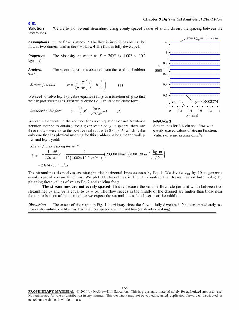
9-51 Solution We are to plot several streamlines using evenly spaced values of and discuss the spacing between the streamlines. Assumptions 1 The flow is steady. 2 The flow is incompressible. 3 The flow is two-dimensional in the x-y plane. 4 The flow is fully developed. Properties The viscosity of water at T = 20oC is 1.002 10-3 kg/(ms). Analysis The stream function is obtained from the result of Problem 9-43,
Stream function: 3 21
2 3 2
dP y yh
dx
(1)
We need to solve Eq. 1 (a cubic equation) for y as a function of so that we can plot streamlines. First we re-write Eq. 1 in standard cubic form,
Standard cubic form: 3 23 60
2 /
hy y
dP dx
(2)
We can either look up the solution for cubic equations or use Newton’s iteration method to obtain y for a given value of . In general there are three roots – we choose the positive real root with 0 < y < h, which is the only one that has physical meaning for this problem. Along the top wall, y = h, and Eq. 1 yields
Stream function along top wall:
33 3top 23
3 2
1 1 kg m20,000 N/m 0.00120 m
12 s N12 1.002 10 kg/m s
2.874 10 m /s
dPh
dx
The streamlines themselves are straight, flat horizontal lines as seen by Eq. 1. We divide top by 10 to generate evenly spaced stream functions. We plot 11 streamlines in Fig. 1 (counting the streamlines on both walls) by plugging these values of into Eq. 2 and solving for y. The streamlines are not evenly spaced. This is because the volume flow rate per unit width between two streamlines 2 and 1 is equal to 2 – 1. The flow speeds in the middle of the channel are higher than those near the top or bottom of the channel, so we expect the streamlines to be closer near the middle. Discussion The extent of the x axis in Fig. 1 is arbitrary since the flow is fully developed. You can immediately see from a streamline plot like Fig. 1 where flow speeds are high and low (relatively speaking).
0
0.2
0.4
0.6
0.8
1
1.2
0 0.2 0.4 0.6 0.8 1
x (mm)
y (mm)
= 0 = 0.0002874
= top = 0.002874
FIGURE 1 Streamlines for 2-D channel flow with evenly spaced values of stream function. Values of are in units of m2/s.

Chapter 9 Differential Analysis of Fluid Flow
9-32 PROPRIETARY MATERIAL. © 2014 by McGraw-Hill Education. This is proprietary material solely for authorized instructor use. Not authorized for sale or distribution in any manner. This document may not be copied, scanned, duplicated, forwarded, distributed, or posted on a website, in whole or part.
9-52 Solution We are to calculate the volume flow rate and average speed of air being sucked through a sampling probe.
Assumptions 1 The flow is steady. 2 The flow is incompressible. 3 The flow is two-dimensional.
Analysis For 2-D incompressible flow the difference in the value of the stream function between two streamlines is equal to the volume flow rate per unit width between the two streamlines. Thus, Volume flow rate through the sampling probe:
/sm 0.00225 3 /sm 0.0022515m 0.0395/sm )093.0(0.150 32Wiu V (1)
The average speed of air in the probe is obtained by dividing volume flow rate by cross-sectional area, Average speed through the sampling probe:
m/s 12.4 m/s 4454.12m) m)(0.0395 (0.00458
/sm 0.022515 3
avg hWV
V (2)
Discussion Notice that the streamlines inside the probe are more closely packed than are those outside the probe because the flow speed is higher inside the probe.
9-53 Solution We are to sketch streamlines for the case of a sampling probe with too little suction, and we are to name this type of sampling and label the lower and upper dividing streamlines.
Analysis If the suction were too weak, the volume flow rate through the probe would be too low and the average air speed through the probe would be lower than that of the air stream. The dividing streamlines would diverge outward rather than inward as sketched in Fig. 1. We would call this type of sampling subisokinetic sampling.
Discussion We have drawn the streamlines inside the probe further apart than those in the air stream because the flow speed is lower inside the probe.
Vfreestream V
Sampling probe
Dividing streamlines
= l
= u
h
Vavg
FIGURE 1 Streamlines for subisokinetic sampling.
Chapter 9 Differential Analysis of Fluid Flow
9-33 PROPRIETARY MATERIAL. © 2014 by McGraw-Hill Education. This is proprietary material solely for authorized instructor use. Not authorized for sale or distribution in any manner. This document may not be copied, scanned, duplicated, forwarded, distributed, or posted on a website, in whole or part.
9-54 Solution We are to calculate the speed of the air stream of a previous problem.
Assumptions 1 The flow is steady. 2 The flow is incompressible. 3 The flow is two-dimensional.
Analysis In the air stream far upstream of the probe,
Volume flow rate per unit width: freestream freestreamu l u l u lV y V y V y yW
V
(1)
By definition of streamlines, the volume flow rate between the two dividing streamlines must be the same as that through the probe itself. We know the volume flow rate through the probe from the results of the previous problem. The value of the stream function on the lower and upper dividing streamlines are the same as those of the previous problem, namely l = 0.093 m2/s and u = 0.150 m2/s respectively. We also know yu – yl from the information given here. Thus, Eq. 1 yields
Freestream speed:
m/s 9.13
m/s 134624.9m 0.00624
/sm 0.093)(0.150 2
stream freeiu
iu
yyV
(2)
Discussion We verify by these calculations that the sampling is superisokinetic (average speed through the probe is higher than that of the upstream air stream).
9-55 Solution For a given stream function we are to generate expressions for the velocity components. Assumptions 1 The flow is steady. 2 The flow is two-dimensional in the r- plane. Analysis We differentiate to find the velocity components in cylindrical coordinates,
Radial velocity component: 2
2
1cos 1
au V
r r
Tangential velocity component: 2
2sin 1
au V
r r
Discussion The radial velocity component is zero at the cylinder surface (r = a), but the tangential velocity component is not. In other words, this approximation does not satisfy the no-slip boundary condition along the cylinder surface. See Chap. 10 for a more detailed discussion about such approximations.

Chapter 9 Differential Analysis of Fluid Flow
9-34 PROPRIETARY MATERIAL. © 2014 by McGraw-Hill Education. This is proprietary material solely for authorized instructor use. Not authorized for sale or distribution in any manner. This document may not be copied, scanned, duplicated, forwarded, distributed, or posted on a website, in whole or part.
9-56 Solution We are to verify that the given satisfies the continuity equation, and we are to discuss any restrictions.
Assumptions 1 The flow is steady. 2 The flow is incompressible. 3 The flow is axisymmetric ( is a function of r and z only). Analysis We plug the given velocity components into the axisymmetric continuity equation,
2 2
11 1 1
0r zru u z r r
r r z r r z r r z z r
Thus we see that continuity is satisfied by the given stream function. The only restriction on is that must be a smooth function of r and z. Discussion For a smooth function of two variables, the order of differentiation does not matter.
9-57 Solution For a given velocity field we are to generate an expression for .
Assumptions 1 The flow is steady. 2 The flow is incompressible. 3 The flow is two-dimensional in the x-y plane.
Analysis We start by picking one of the two definitions of the stream function (it doesn’t matter which part we choose – the solution will be identical).
cosu Vy
(1)
Next we integrate Eq. 1 with respect to y, noting that this is a partial integration and we must add an arbitrary function of the other variable, x, rather than a simple constant of integration.
cosyV g x (2)
Now we choose the other part of the definition of , differentiate Eq. 2, and rearrange as follows:
v g xx
(3)
where g(x) denotes dg/dx since g is a function of only one variable, x. We now have two expressions for velocity component v, the given equation and Eq. 3. We equate these and integrate with respect to x to find g(x),
sin sin sinv V g x g x V g x xV C (4)
Note that here we have added an arbitrary constant of integration C since g is a function of x only. Finally, plugging Eq. 4 into Eq. 2 yields the final expression for ,
Stream function: cos sinV y x C (5)
Constant C is arbitrary; it is common to set it to zero, although it can be set to any desired value.
Discussion You can verify by differentiating that Eq. 5 yields the correct values of u and v.

Chapter 9 Differential Analysis of Fluid Flow
9-35 PROPRIETARY MATERIAL. © 2014 by McGraw-Hill Education. This is proprietary material solely for authorized instructor use. Not authorized for sale or distribution in any manner. This document may not be copied, scanned, duplicated, forwarded, distributed, or posted on a website, in whole or part.
9-58 Solution For a given stream function, we are to calculate the velocity components and verify incompressibility.
Assumptions 1 The flow is steady. 2 The flow is incompressible (this assumption is to be verified). 3 The flow is two-dimensional in the x-y plane, implying that w = 0 and neither u nor v depend on z.
Analysis (a) We use the definition of to obtain expressions for u and v.
Velocity components: 2 2u bx cy v ax byy x
(1)
(b) We check if the incompressible continuity equation in the x-y plane is satisfied by the velocity components of Eq. 1,
Incompressible continuity:
b b
u v w
x y z
0
0 0b b (2)
We conclude that the flow is indeed incompressible.
Discussion Since is a smooth function of x and y, it automatically satisfies the continuity equation by its definition. Equation 2 confirms this. If it did not, we would go back and look for an algebra mistake somewhere.
9-59 Solution We are to plot several streamlines for a given velocity field. Analysis We re-write the stream function equation of the previous problem with all the terms on one side,
2 2 0cy bxy ax (1)
For any constant value of (along a streamline), Eq. 1 is in a form that enables us to use the quadratic rule to solve for y as a function of x,
Equation for a streamline: 2 2 24
2
bx b x c axy
c
(2)
We plot the streamlines in Fig. 1. For each value of there are two curves – one for the positive root and one for the negative root of Eq. 2. There is symmetry about a diagonal line through the origin. The streamlines appear to be hyperbolae. We determine the flow direction by plugging in a couple values of x and y and calculating the velocity components; e.g., at x = 1 m and y = 3 m, u = 2.7 m/s and v = 4.9 m/s. The flow at this point is in the upper right direction. Similarly, at x = 1 m and y = -2 m, u = -3.3 m/s and v = -1.6 m/s. The flow at this point is in the lower left direction. Discussion This flow may not represent any particular physical flow field, but it produces an interesting flow pattern.
-4
-3
-2
-1
0
1
2
3
4
-2 -1 0 1 2
x (m)
y (m)
= 0
= 6
= 6
= 0
FIGURE 1 Streamlines for a given velocity field. Values of are in units of m2/s.

Chapter 9 Differential Analysis of Fluid Flow
9-36 PROPRIETARY MATERIAL. © 2014 by McGraw-Hill Education. This is proprietary material solely for authorized instructor use. Not authorized for sale or distribution in any manner. This document may not be copied, scanned, duplicated, forwarded, distributed, or posted on a website, in whole or part.
9-60 Solution For a given stream function, we are to calculate the velocity components and verify incompressibility.
Assumptions 1 The flow is steady. 2 The flow is incompressible. 3 The flow is two-dimensional in the x-y plane, implying that w = 0 and neither u nor v depend on z.
Analysis (a) We use the definition of to obtain expressions for u and v.
Velocity components: 2 2u by dx v ax c dyy x
(1)
(b) We check if the incompressible continuity equation in the x-y plane is satisfied by the velocity components of Eq. 1,
Incompressible continuity:
d d
u v w
x y z
0
0 0d d (2)
We conclude that the flow is indeed incompressible.
Discussion Since is a smooth function of x and y, it automatically satisfies the continuity equation by its definition. Eq. 2 confirms this. If it did not, we would go back and look for an algebra mistake somewhere.
9-61 Solution We are to make up a stream function (x,y), calculate the velocity components and verify incompressibility.
Assumptions 1 The flow is steady. 2 The flow is incompressible. 3 The flow is two-dimensional in the x-y plane.
Analysis Every student should have a different stream function. He or she then takes the derivatives with respect to y and x to find u and v. The student should then plug his/her velocity components into the incompressible continuity equation. Continuity will be satisfied regardless of (x,y), provided that (x,y) is a smooth function of x and y.
Discussion As long as is a smooth function of x and y, it automatically satisfies the continuity equation by its definition.
Chapter 9 Differential Analysis of Fluid Flow
9-37 PROPRIETARY MATERIAL. © 2014 by McGraw-Hill Education. This is proprietary material solely for authorized instructor use. Not authorized for sale or distribution in any manner. This document may not be copied, scanned, duplicated, forwarded, distributed, or posted on a website, in whole or part.
9-62 Solution We are to calculate the percentage of flow going through one branch of a branching duct.
Assumptions 1 The flow is steady. 2 The flow is incompressible. 3 The flow is two-dimensional in the x-y plane.
Analysis For 2-D incompressible flow the difference in the value of the stream function between two streamlines is equal to the volume flow rate per unit width between the two streamlines. Thus,
Main branch: 2 2
upper wall lower wall
main
m m4.35 2.03 2.32
s sW
V (1)
Similary, in the upper branch,
Upper branch: s
m 1.25
s
m)10.3(4.35
22
lbranch walupper wall
upper
W
V (2)
On a percentage basis, the percentage of volume flow through the upper branch is calculated as
53.9%
53879.0
s
m 2.32
s
m 1.25
2
2
main
upper
main
upper
W
W
V
V
V
V
(3)
Discussion No dimensions are given, so it is not possible to calculate velocities.

Chapter 9 Differential Analysis of Fluid Flow
9-38 PROPRIETARY MATERIAL. © 2014 by McGraw-Hill Education. This is proprietary material solely for authorized instructor use. Not authorized for sale or distribution in any manner. This document may not be copied, scanned, duplicated, forwarded, distributed, or posted on a website, in whole or part.
9-63 Solution We are to calculate duct height h for a given average velocity through a duct and values of stream function along the duct walls.
Assumptions 1 The flow is steady. 2 The flow is incompressible. 3 The flow is two-dimensional in the x-y plane.
Analysis The volume flow rate through the main branch of the duct is equal to the average velocity times the cross-sectional area of the duct,
Volume flow rate: avgV WhV (1)
We solve for h in Eq. 1, using the results of the previous problem,
Duct height: 2
avg main
1 1 m 100 cm2.32 17.3134 cm
m s m13.4s
hV W
17.3 cm
V (2)
An alternative way to solve for height h is to assume uniform flow in the main branch, for which = Vavgy. We take the difference between at the top of the duct and at the bottom of the duct to find h,
upper wall lower wall avg upper wall avg lower wall avg upper wall lower wall avgV y V y V y y V h
Thus,
Duct height:
2
upper wall lower wall
avg
m4.35 2.03 100 cms 17.3134 cm
m m13.4s
hV
17.3 cm (3)
You can see that we get the same result as that of Eq. 2.
Discussion The result is correct even if the velocity profile through the duct is not uniform, since we have used the average velocity in our calculations.
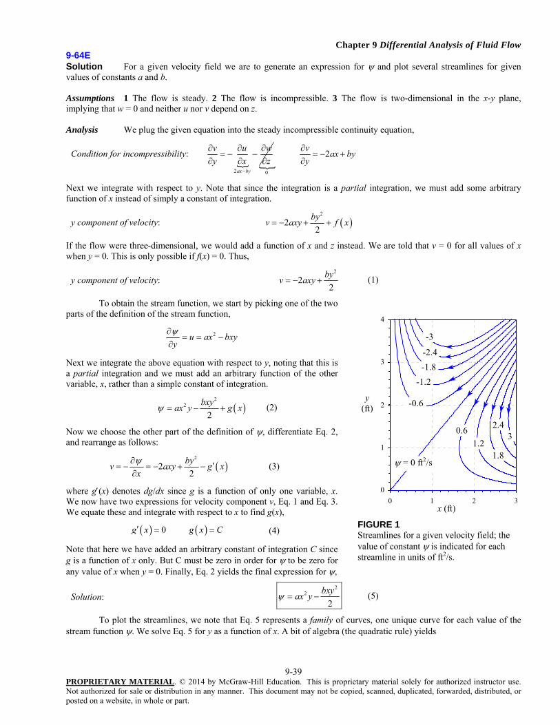
Chapter 9 Differential Analysis of Fluid Flow
9-39 PROPRIETARY MATERIAL. © 2014 by McGraw-Hill Education. This is proprietary material solely for authorized instructor use. Not authorized for sale or distribution in any manner. This document may not be copied, scanned, duplicated, forwarded, distributed, or posted on a website, in whole or part.
9-64E Solution For a given velocity field we are to generate an expression for and plot several streamlines for given values of constants a and b. Assumptions 1 The flow is steady. 2 The flow is incompressible. 3 The flow is two-dimensional in the x-y plane, implying that w = 0 and neither u nor v depend on z. Analysis We plug the given equation into the steady incompressible continuity equation,
Condition for incompressibility:
2ax by
v u w
y x z
0
2v
ax byy
Next we integrate with respect to y. Note that since the integration is a partial integration, we must add some arbitrary function of x instead of simply a constant of integration.
y component of velocity: 2
22
byv axy f x
If the flow were three-dimensional, we would add a function of x and z instead. We are told that v = 0 for all values of x when y = 0. This is only possible if f(x) = 0. Thus,
y component of velocity: 2
22
byv axy (1)
To obtain the stream function, we start by picking one of the two parts of the definition of the stream function,
2u ax bxyy
Next we integrate the above equation with respect to y, noting that this is a partial integration and we must add an arbitrary function of the other variable, x, rather than a simple constant of integration.
2
2
2
bxyax y g x (2)
Now we choose the other part of the definition of , differentiate Eq. 2, and rearrange as follows:
2
22
byv axy g x
x
(3)
where g(x) denotes dg/dx since g is a function of only one variable, x. We now have two expressions for velocity component v, Eq. 1 and Eq. 3. We equate these and integrate with respect to x to find g(x),
0 g x g x C (4)
Note that here we have added an arbitrary constant of integration C since g is a function of x only. But C must be zero in order for to be zero for any value of x when y = 0. Finally, Eq. 2 yields the final expression for ,
Solution: 2
2
2
bxyax y (5)
To plot the streamlines, we note that Eq. 5 represents a family of curves, one unique curve for each value of the stream function . We solve Eq. 5 for y as a function of x. A bit of algebra (the quadratic rule) yields
0
1
2
3
4
0 1 2 3
= 0 ft2/s
x (ft)
y (ft)
1.8
2.43
1.2
0.6
-0.6
-1.2
-1.8
-2.4
-3
FIGURE 1 Streamlines for a given velocity field; the value of constant is indicated for each streamline in units of ft2/s.

Chapter 9 Differential Analysis of Fluid Flow
9-40 PROPRIETARY MATERIAL. © 2014 by McGraw-Hill Education. This is proprietary material solely for authorized instructor use. Not authorized for sale or distribution in any manner. This document may not be copied, scanned, duplicated, forwarded, distributed, or posted on a website, in whole or part.
Equation for streamlines: 2 2 4 2ax a x bx
ybx
(6)
For the given values of constants a and b, we plot Eq. 6 for several values of in Fig. 1; these curves of constant are streamlines of the flow. Note that both the positive and negative roots of Eq. 6 are required to plot each streamline. The direction of the flow is found by calculating u and v at some point in the flow field. We pick x = 2 ft, y = 2 ft, where u = 1.2 ft/s and v = 2.1 ft/s. This indicates flow to the lower left near this location. We fill in the rest of the arrows in Fig. 1 to be consistent. We see that the flow enters from the upper right, and splits into two parts – one to the lower right and one to the upper left. Discussion It is always a good idea to check your algebra. In this example, you should differentiate Eq. 5 to verify that the velocity components of the given equation are obtained.
Chapter 9 Differential Analysis of Fluid Flow
9-41 PROPRIETARY MATERIAL. © 2014 by McGraw-Hill Education. This is proprietary material solely for authorized instructor use. Not authorized for sale or distribution in any manner. This document may not be copied, scanned, duplicated, forwarded, distributed, or posted on a website, in whole or part.
9-65 Solution We are to generate an expression for the stream function that describes a given velocity field. Assumptions 1 The flow is steady. 2 The flow is incompressible. 3 The flow is axisymmetric ( is a function of r and z only). Analysis The r and z velocity components from Problem 9-34 are
Velocity field: ,exit ,entrance ,exit ,entrance,entrance
2z z z z
r z z
u u u uru u u z
L L
(1)
To generate the stream function we use the definition of for steady, incompressible, axisymmetric flow,
Axisymmetric stream function: 1 1
r zu ur z r r
(2)
We choose one of the definitions of Eq. 2 to integrate. We pick the second one,
Integration:
,exit ,entrance,entrance
2,exit ,entrance
,entrance ( )2
z zz z
z zz
u uru dr r u z dr
L
u uru z f z
L
(3)
We added a function of z instead of a constant of integration since this is a partial integration. Now we take the z derivative of Eq. 3 and use the other half of Eq. 2,
Differentiation: ,exit ,entrance1 1( )
2z z
r
u uru f z
r z L r
(4)
We equate Eq. 4 to the known value of ur from Eq. 1,
Comparison:
,exit ,entrance ,exit ,entrance1( ) or ( ) 0
2 2z z z z
r
u u u ur ru f z f z
L r L
(5)
Since f is a function of z only, integration of Eq. 5 yields f(z) = constant. The final result is thus
Stream function: 2
,exit ,entrance,entrance constant
2z z
z
u uru z
L
(6)
Discussion The constant of integration can be any value since velocity components are determined by taking derivatives of the stream function.

Chapter 9 Differential Analysis of Fluid Flow
9-42 PROPRIETARY MATERIAL. © 2014 by McGraw-Hill Education. This is proprietary material solely for authorized instructor use. Not authorized for sale or distribution in any manner. This document may not be copied, scanned, duplicated, forwarded, distributed, or posted on a website, in whole or part.
9-66E Solution We are to calculate the axial speed at the entrance and exit of the nozzle, and we are to plot several streamlines for a given axisymmetric flow field. Assumptions 1 The flow is steady. 2 The flow is incompressible. 3 The flow is axisymmetric ( is a function of r and z only). Analysis (a) Since uz is not a function of radius, the axial velocity profile across a cross section of the nozzle is uniform. (This is consistent with the assumption that frictional effects along the nozzle walls are neglected.) Thus, at any cross section the axial speed is equal to the volume flow rate divided by cross-sectional area,
Entrance axial speed:
23
,entrance 2 2entrance
gal4 2.04 0.1337 ft 12 in minmin
gal ft 60 s0.50 inzu
D
ft3.268
s
V
(1)
Similarly,
Exit axial speed: ,exit 2exit
4zu
D
ft41.69
s
V (2)
(b) We use the stream function developed in Problem 9-61. Setting the constant to zero for simplicity, we have
Stream function: 2
,exit ,entrance,entrance2
z zz
u uru z
L
(3)
We solve Eq. 3 for r as a function of z and plot several streamlines in Fig. 1,
Streamlines: ,exit ,entrance
,entrance
2
z zz
ru u
u zL
(4)
At the nozzle entrance (z = 0), the wall is at r = Dentrance/2 = 0.25 inches. Eq. 3 yields wall = 0.0007073 ft3/s for the streamline that passes through this point. This streamline thus represents the shape of the nozzle wall, and we have designed the nozzle shape. Discussion You can verify that the diameter between the outermost streamlines varies from Dentrance to Dexit.
-0.25
-0.2
-0.15
-0.1
-0.05
0
0.05
0.1
0.15
0.2
0.25
0 0.5 1 1.5 2
z (in)
r (in)
= 0
Nozzle wall
FIGURE 1 Streamlines for flow through an axisymmetric garden hose nozzle. Note that the vertical axis is highly magnified.
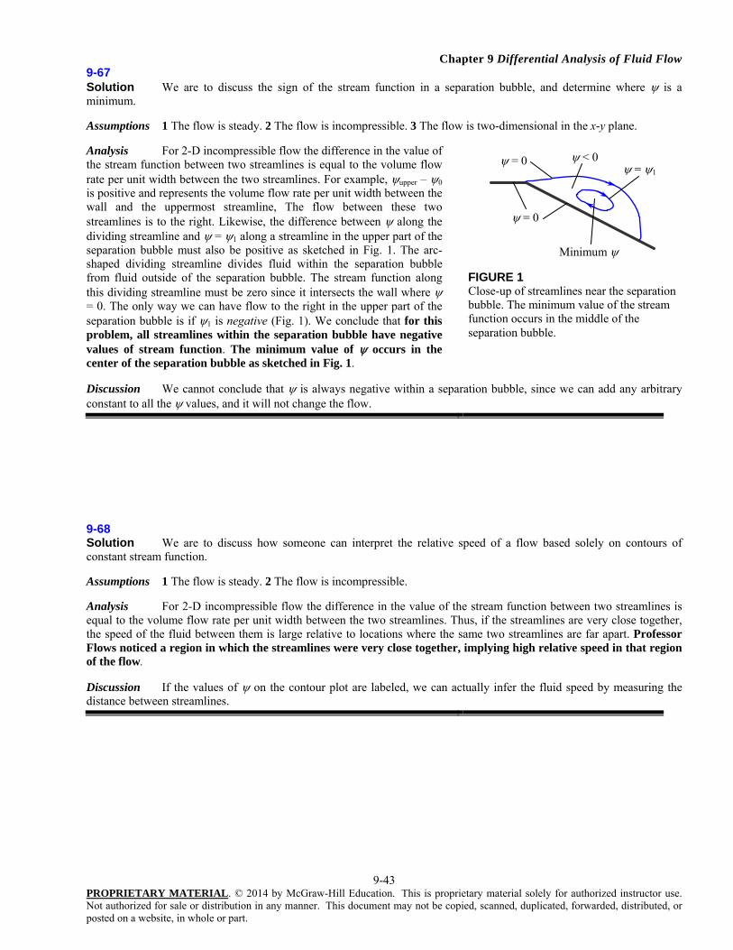
Chapter 9 Differential Analysis of Fluid Flow
9-43 PROPRIETARY MATERIAL. © 2014 by McGraw-Hill Education. This is proprietary material solely for authorized instructor use. Not authorized for sale or distribution in any manner. This document may not be copied, scanned, duplicated, forwarded, distributed, or posted on a website, in whole or part.
9-67 Solution We are to discuss the sign of the stream function in a separation bubble, and determine where is a minimum.
Assumptions 1 The flow is steady. 2 The flow is incompressible. 3 The flow is two-dimensional in the x-y plane.
Analysis For 2-D incompressible flow the difference in the value of the stream function between two streamlines is equal to the volume flow rate per unit width between the two streamlines. For example, upper – 0 is positive and represents the volume flow rate per unit width between the wall and the uppermost streamline, The flow between these two streamlines is to the right. Likewise, the difference between along the dividing streamline and = 1 along a streamline in the upper part of the separation bubble must also be positive as sketched in Fig. 1. The arc-shaped dividing streamline divides fluid within the separation bubble from fluid outside of the separation bubble. The stream function along this dividing streamline must be zero since it intersects the wall where = 0. The only way we can have flow to the right in the upper part of the separation bubble is if 1 is negative (Fig. 1). We conclude that for this problem, all streamlines within the separation bubble have negative values of stream function. The minimum value of occurs in the center of the separation bubble as sketched in Fig. 1.
Discussion We cannot conclude that is always negative within a separation bubble, since we can add any arbitrary constant to all the values, and it will not change the flow.
9-68 Solution We are to discuss how someone can interpret the relative speed of a flow based solely on contours of constant stream function.
Assumptions 1 The flow is steady. 2 The flow is incompressible.
Analysis For 2-D incompressible flow the difference in the value of the stream function between two streamlines is equal to the volume flow rate per unit width between the two streamlines. Thus, if the streamlines are very close together, the speed of the fluid between them is large relative to locations where the same two streamlines are far apart. Professor Flows noticed a region in which the streamlines were very close together, implying high relative speed in that region of the flow.
Discussion If the values of on the contour plot are labeled, we can actually infer the fluid speed by measuring the distance between streamlines.
= 0
= 0
= 1
< 0
Minimum
FIGURE 1 Close-up of streamlines near the separation bubble. The minimum value of the stream function occurs in the middle of the separation bubble.
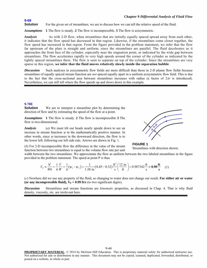
Chapter 9 Differential Analysis of Fluid Flow
9-44 PROPRIETARY MATERIAL. © 2014 by McGraw-Hill Education. This is proprietary material solely for authorized instructor use. Not authorized for sale or distribution in any manner. This document may not be copied, scanned, duplicated, forwarded, distributed, or posted on a website, in whole or part.
9-69 Solution For the given set of streamlines, we are to discuss how we can tell the relative speed of the fluid.
Assumptions 1 The flow is steady. 2 The flow is incompressible. 3 The flow is axisymmetric.
Analysis As with 2-D flow, when streamlines that are initially equally spaced spread away from each other, it indicates that the flow speed has decreased in that region. Likewise, if the streamlines come closer together, the flow speed has increased in that region. From the figure provided in the problem statement, we infer that the flow far upstream of the plate is straight and uniform, since the streamlines are parallel. The fluid decelerates as it approaches the front face of the cylinder, especially near the stagnation point, as indicated by the wide gap between streamlines. The flow accelerates rapidly to very high speeds around the corner of the cylinder as indicated by the tightly spaced streamlines there. The flow is seen to separate on top of the cylinder. Since the streamlines are very sparse in this region, we infer that the fluid moves relatively slowly inside the separation bubble.
Discussion Such analyses in axisymmetric flow fields are more difficult than those in 2-D planar flow fields because streamlines of equally spaced stream function are not spaced equally apart in a uniform axisymmetric flow field. This is due to the fact that the cross-sectional area between streamlines increases with radius (a factor of 2r is introduced). Nevertheless, we can still tell where the flow speeds up and slows down in this example.
9-70E Solution We are to interpret a streamline plot by determining the direction of flow and by estimating the speed of the flow at a point.
Assumptions 1 The flow is steady. 2 The flow is incompressible 3 The flow is two-dimensional.
Analysis (a) We must tilt our heads nearly upside down to see an increase in stream function in the mathematically positive manner. In other words, since increases in the downward direction, the flow is to the lower left, following our left side rule. Arrows are drawn in Fig. 1.
(b) For 2-D incompressible flow the difference in the value of the stream function between two streamlines is equal to the volume flow rate per unit width between the two streamlines. We approximate the flow as uniform between the two labeled streamlines in the figure provided in the problem statement. The speed at point P is thus
2
P 1 2
1 1 1 ft 12 in ft0.45 0.32 0.987342
1.58 in s ft s
VV
Wh h W h
ft0.99
s
V (1)
(c) Nowhere did we use any property of the fluid, so changing to water does not change our result. For either air or water (or any incompressible fluid), VP = 0.99 ft/s (to two significant digits).
Discussion Streamlines and stream functions are kinematic properties, as discussed in Chap. 4. That is why fluid density, viscosity, etc. are irrelevant here.
P h
FIGURE 1 Streamlines with direction shown.

Chapter 9 Differential Analysis of Fluid Flow
9-45 PROPRIETARY MATERIAL. © 2014 by McGraw-Hill Education. This is proprietary material solely for authorized instructor use. Not authorized for sale or distribution in any manner. This document may not be copied, scanned, duplicated, forwarded, distributed, or posted on a website, in whole or part.
9-71 Solution We are to find the primary dimensions and primary units of the compressible stream function. Analysis From the given definition, we see that is the product of a density, a velocity, and a length,
Primary dimensions of : 3
mass length mlength
time Ltlength
The primary units of are kg/(ms) (SI) and lbm/(ft s) (English).
Discussion Ironically, although the stream function is often applied to potential flows where viscosity is not a parameter, has the same units as .
9-72 Solution We are to generate an expression for the compressible stream function for a given flow field. Assumptions 1 The flow is steady. 2 The flow is two-dimensional in the x-y plane. Analysis We start by picking one of the two definitions of the compressible stream function (it doesn’t matter which part we choose – the solution will be identical).
21 1 1 1 1 1u u uu C x u C x u C u C x C C x
y
(1)
Next we integrate Eq. 1 with respect to y, noting that this is a partial integration and we must add an arbitrary function of the other variable, x, rather than a simple constant of integration.
21 1 1 1u uu y C u C xy C C x y g x (2)
Now we choose the other part of the definition of , differentiate Eq. 2, and rearrange as follows:
1 1 2u uv C u C y C C xy g xx
(3)
where g(x) denotes dg/dx since g is a function of only one variable, x. We now have two expressions for v, Eq. 3 and the value computed from the known density and velocity, i.e.
1 1 2u uv C u C y C C xy (4)
We equate Eqs. 3 and 4 and integrate with respect to x to find g(x),
0 g x g x C (5)
Note that here we have added an arbitrary constant of integration C since g is a function of x only. Plugging Eq. 5 into Eq. 2 yields
21 1 1 1u uu y C u C xy C C x y C (6)
We determine constant C by setting = 0 at y = 0 in Eq. 6, yielding C = 0. Thus the final expression for the compressible stream function is
Compressible stream function: 21 1 1 1u uu y C u C xy C C x y (7)
Discussion You can verify by differentiating that Eq. 7 yields the correct values of u and v.

Chapter 9 Differential Analysis of Fluid Flow
9-46 PROPRIETARY MATERIAL. © 2014 by McGraw-Hill Education. This is proprietary material solely for authorized instructor use. Not authorized for sale or distribution in any manner. This document may not be copied, scanned, duplicated, forwarded, distributed, or posted on a website, in whole or part.
9-73 Solution We are to generate an expression for the compressible stream function for a given flow field. Assumptions 1 The flow is steady. 2 The flow is two-dimensional in the x-y plane. Analysis We start by picking one of the two definitions of the compressible stream function (it doesn’t matter which part we choose – the solution will be identical).
21 1 1 1 1 1u u uu C x u C x u C u C x C C x
y
(1)
Next we integrate Eq. 1 with respect to y, noting that this is a partial integration and we must add an arbitrary function of the other variable, x, rather than a simple constant of integration.
21 1 1 1u uu y C u C xy C C x y g x (2)
Now we choose the other part of the definition of , differentiate Eq. 2, and rearrange as follows:
1 1 2u uv C u C y C C xy g xx
(3)
where g(x) denotes dg/dx since g is a function of only one variable, x. We now have two expressions for v, Eq. 3 and the value computed from the known density and velocity, i.e.
1 1 2u uv C u C y C C xy (4)
We equate Eqs. 3 and 4 and integrate with respect to x to find g(x),
0 g x g x C (5)
Note that here we have added an arbitrary constant of integration C since g is a function of x only. Plugging Eq. 5 into Eq. 2 yields
21 1 1 1u uu y C u C xy C C x y C (6)
We determine constant C by setting = 0 at y = 0 in Eq. 6, yielding C = 0. Thus the final expression for the compressible stream function is
Compressible stream function: 21 1 1 1u uu y C u C xy C C x y (7)
We solve Eq. 7 for y as a function of x and so that we can plot streamlines,
Equation for plotting streamlines: 2
1 1 1 1u u
yu C u C x C C x
(8)
We plot Eq. 8 in Fig. 1 for several values of , using the values of constants u1, 1, Cu, and C given in Problem 9-21. The agreement with the streamlines of Problem 9-21 is excellent. The streamline starting at x = 0, y = 0.8 m is the top wall of the duct. Therefore the value of at the top wall of the diverging duct is found be setting at x = 0 and y = 0.8 m,
at the top wall: , top 1 1 3
kg m0.85 300 0.8 m
smu y
kg204
m s (9)
Discussion You can verify by differentiating that Eq. 9 yields the correct values of u and v.
0
0.5
1
1.5
2
0 0.5 1 1.5 2x
y
Top wall, kg
204m s
Symmetry line, = 0
FIGURE 1 Streamlines for a diverging duct.
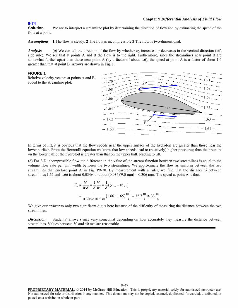
Chapter 9 Differential Analysis of Fluid Flow
9-47 PROPRIETARY MATERIAL. © 2014 by McGraw-Hill Education. This is proprietary material solely for authorized instructor use. Not authorized for sale or distribution in any manner. This document may not be copied, scanned, duplicated, forwarded, distributed, or posted on a website, in whole or part.
9-74 Solution We are to interpret a streamline plot by determining the direction of flow and by estimating the speed of the flow at a point. Assumptions 1 The flow is steady. 2 The flow is incompressible 3 The flow is two-dimensional. Analysis (a) We can tell the direction of the flow by whether increases or decreases in the vertical direction (left side rule). We see that at points A and B the flow is to the right. Furthermore, since the streamlines near point B are somewhat further apart than those near point A (by a factor of about 1.6), the speed at point A is a factor of about 1.6 greater than that at point B. Arrows are drawn in Fig. 1.
In terms of lift, it is obvious that the flow speeds near the upper surface of the hydrofoil are greater than those near the lower surface. From the Bernoulli equation we know that low speeds lead to (relatively) higher pressures; thus the pressure on the lower half of the hydrofoil is greater than that on the upper half, leading to lift.
(b) For 2-D incompressible flow the difference in the value of the stream function between two streamlines is equal to the volume flow rate per unit width between the two streamlines. We approximate the flow as uniform between the two streamlines that enclose point A in Fig. P9-70. By measurement with a ruler, we find that the distance between streamlines 1.65 and 1.66 is about 0.034c, or about (0.034)(9.0 mm) = 0.306 mm. The speed at point A is thus
A 1.66 1.65
2
3
1 1
1 m m 1.66 1.65 32.7
s s0.306 10 m
VW W
m33.
s
V V
We give our answer to only two significant digits here because of the difficulty of measuring the distance between the two streamlines. Discussion Students’ answers may vary somewhat depending on how accurately they measure the distance between streamlines. Values between 30 and 40 m/s are reasonable.
FIGURE 1 Relative velocity vectors at points A and B, added to the streamline plot.
1.70 A
1.62
c
1.60
1.64
1.66
1.68
1.71
1.63
1.61
1.65
1.67
1.69
B

Chapter 9 Differential Analysis of Fluid Flow
9-48 PROPRIETARY MATERIAL. © 2014 by McGraw-Hill Education. This is proprietary material solely for authorized instructor use. Not authorized for sale or distribution in any manner. This document may not be copied, scanned, duplicated, forwarded, distributed, or posted on a website, in whole or part.
9-75 Solution We are to interpret a streamline plot by determining the direction of flow and by estimating the speed of the flow at a point. Assumptions 1 The flow is steady (time-averaged). 2 The flow is incompressible 3 The flow is two-dimensional. Properties The density of air at T = 20oC is 1.18 kg/m3. Analysis (a) We can tell the direction of the flow by whether increases or decreases in the vertical direction (left side rule). We see that at point A, the flow is to the left, while at point B the flow is to the right. Furthermore, since the streamlines near point B are much closer together than those near point A (by a factor of about five), the speed at point B is a factor of about five greater than that at point A. Arrows are drawn in Fig. 1.
(b) For 2-D incompressible flow the difference in the value of the compressible stream function between two streamlines is equal to the mass flow rate per unit width between the two streamlines. We approximate the flow as uniform between the two streamlines that enclose point B in Fig. P9-71. By measurement with a ruler, we find that the distance between streamlines 5 and 6 is about h/10, or about 0.10 m. The speed at point B is thus
B 6 5
3
1 1 1 kg6 5
kg m s1.18 0.10 m
m
m mV
W W
m8.5
s
(1)
We are only accurate to one digit here because of the difficulty of measuring the distance between the two streamlines. We give our final result as VB = 8 or 9 m/s. Discussion Students’ answers may vary considerably depending on how accurately they measure the distance between streamlines.
1 A
2 h
h
3 4 6 10 B
FIGURE 1 Relative velocity vectors at points A and B, added to the streamline plot.

Chapter 9 Differential Analysis of Fluid Flow
9-49 PROPRIETARY MATERIAL. © 2014 by McGraw-Hill Education. This is proprietary material solely for authorized instructor use. Not authorized for sale or distribution in any manner. This document may not be copied, scanned, duplicated, forwarded, distributed, or posted on a website, in whole or part.
9-76 Solution We are to determine the value of the stream function along the positive y axis and the negative x axis for the case of a line source at the origin. Assumptions 1 The flow is steady. 2 The flow is incompressible. 3 The flow is two-dimensional in the x-y or r- plane. Analysis For 2-D incompressible flow the difference in the value of the stream function between two streamlines is equal to the volume flow rate per unit width between the two streamlines. Let us take the arc of the circle of radius r between the positive x axis and the positive y axis of the figure provided with the problem statement. The volume flow rate
per unit width through this arc is one-fourth of / LV , the total volume flow rate per unit width, since the arc spans exactly one-fourth of the circumference of the circle.
positive axis positive axis
1
4y x L
V (1)
Since = 0 along the positive x axis, we conclude that
along positive y axis: positive axis
1
4y L
V (2)
Similarly, the volume flow rate through the top half of the circle is half of the total volume flow rate and we conclude that
along negative x axis: negative axis
1
2y L
V (3)
Discussion Some CFD codes use as a variable, and we thus need to specify the value of along boundaries of the computational domain. Simple calculations such as this are useful in these situations.
9-77 Solution We are to determine the value of the stream function along the positive y axis and the negative x axis for the case of a line sink at the origin. Assumptions 1 The flow is steady. 2 The flow is incompressible. 3 The flow is two-dimensional in the x-y or r- plane. Analysis Everything is the same as in Problem 9-59 except that the flow direction is reversed everywhere. The volume flow rate per unit width through the arc of radius r between the positive x axis and the positive y axis of Fig. P9-59
is now negative one-fourth of / LV since the flow is now mathematically negative.
positive axis positive axis
1
4y x L
V (1)
Since = 0 along the positive x axis, we conclude that
along positive y axis: positive axis
1
4y L
V (2)
Similarly, the volume flow rate through the top half of the circle is half of the total volume flow rate and is negative. We conclude that
along negative x axis: negative axis
1
2x L
V (3)
Discussion We need to be careful of the sign of .

Chapter 9 Differential Analysis of Fluid Flow
9-50 PROPRIETARY MATERIAL. © 2014 by McGraw-Hill Education. This is proprietary material solely for authorized instructor use. Not authorized for sale or distribution in any manner. This document may not be copied, scanned, duplicated, forwarded, distributed, or posted on a website, in whole or part.
Linear Momentum Equation, Boundary Conditions, and Applications 9-78C Solution We are to define mechanical pressure and discuss its application. Analysis Mechanical pressure is the mean normal stress acting inwardly on a fluid element. For an incompressible fluid, the density is constant and therefore we have no equation of state available for calculation of the thermodynamic pressure. In fact, thermodynamic pressure cannot even be defined for an incompressible fluid. Fluid elements and surfaces still “feel” a pressure, however, and this pressure is the so-called mechanical pressure. Discussion When dealing with incompressible fluid flows, pressure variable P is always interpreted as the mechanical pressure Pm.
9-79C Solution We are to describe the constitutive equations and name the equation to which they are applied. Analysis The constitutive equations are relationships between the components of the stress tensor and the primary unknowns of the problem, namely pressure and velocity. The constitutive equations enable us to write the components of the stress tensor in Cauchy’s equation in terms of the velocity field and the pressure field. Discussion Cauchy’s equation by itself is useless without the constitutive equations, because we would have too many unknowns for the number of available equations.
9-80C Solution We are to discuss velocity boundary conditions in a stationary and a moving frame of reference for the case of an airplane flying through the air.
Analysis (a) From the stationary frame of reference, V
= airplaneV
on all surfaces of the airplane, (no-slip boundary
condition). Far from the airplane the air is still (V
= 0).
(b) From the reference frame moving with the airplane, V
= 0 on all surfaces, (no-slip boundary condition). Far from the
airplane the air is moving towards the airplane at a speed that is opposite the airplane’s speed (V
= airplaneV
).
Discussion The no-slip condition requires that the fluid velocity equal the airplane velocity everywhere on the airplane surface, regardless of the geometry of the airplane, and regardless of the frame of reference.

Chapter 9 Differential Analysis of Fluid Flow
9-51 PROPRIETARY MATERIAL. © 2014 by McGraw-Hill Education. This is proprietary material solely for authorized instructor use. Not authorized for sale or distribution in any manner. This document may not be copied, scanned, duplicated, forwarded, distributed, or posted on a website, in whole or part.
9-81C Solution We are to discuss the difference between Newtonian fluids and non-Newtonian fluids, and we are to give examples of each. Analysis The main distinction between a Newtonian fluid and a non-Newtonian fluid is that for flow of a Newtonian fluid, shear stress is linearly proportional to shear strain rate, whereas for flow of a non-Newtonian fluid, the relationship between shear stress and shear strain rate is nonlinear. There are many examples of Newtonian fluids. Most pure, common liquids like water, oil, gasoline, alcohol, etc. are Newtonian. Most gases also behave like Newtonian fluids. Non-newtonian fluids include paint, pastes and creams, polymer solutions, cake batter, slurries and colloidal suspensions like quicksand, blood, etc. Discussion The Navier-Stokes equations apply only to Newtonian fluids. For non-Newtonian fluids, you would need to insert nonlinear constitutive equations into Cauchy’s equations in order to obtain a useful differential equation for conservation of linear momentum.
9-82C Solution We are to define or describe each type of fluid. Analysis (a) A viscoelastic fluid is a fluid that returns (either fully or partially) to its original shape after the applied stress is
released. (b) A pseudoplastic fluid is a shear thinning fluid the more the fluid is sheared, the less viscous it becomes. (c) A dilatant fluid is a shear thickening fluid the more the fluid is sheared, the more viscous it becomes. (d) A Bingham plastic fluid is an extreme type of pseudoplastic fluid that requires a finite stress called the yield
stress in order for the fluid to flow at all. Discussion All of the above are examples of non-Newtonian fluids.
9-83C Solution We are to discuss each term, and write the equation as a word equation. Analysis Term I is the net body force acting on the control volume. Term II is the net surface force acting on the control volume. Term III is the net rate of change of linear momentum within the control volume. Term IV is the net rate of outflow of linear momentum through the control surface. In words, the equation can be expressed as: “The total force acting on the control volume is the sum of body forces and surface forces, and is equal to the rate at which momentum changes within the control volume plus the rate at which momentum flows out of the control volume.” Discussion The dimensions of each term in the equation are those of momentum per time. Each term has primary dimensions of {mLt2}.

Chapter 9 Differential Analysis of Fluid Flow
9-52 PROPRIETARY MATERIAL. © 2014 by McGraw-Hill Education. This is proprietary material solely for authorized instructor use. Not authorized for sale or distribution in any manner. This document may not be copied, scanned, duplicated, forwarded, distributed, or posted on a website, in whole or part.
9-84 Solution We are to generate and discuss velocity and pressure boundary conditions for the given flow problem. Assumptions 1 The flow is steady. 2 Surface tension effects are negligibly small.
Analysis We must satisfy the no-slip boundary condition on all tank walls, liquidV
= tankV
. Mathematically, we write ur
= uz = 0 and u = R at r = R (the tank side walls). We also write ur = uz = 0 and u = r at z = 0 (the bottom wall of the tank). We do not specify the pressure along the tank walls. At the free surface P = Patm since the free surface is exposed to atmospheric air. In addition, the vertical and radial components of velocity uz and ur must equal zero at the free surface, but the angular velocity component u is set to u = r at the free surface. We also know that the shear stress at free surface must be zero (negligible shear due to the air). This boundary condition is not needed however since we already know the velocity field. In fact, the velocity field is known right from the start since we are told that the liquid is in solid body rotation: uz = ur = 0 and u = r everywhere. Discussion This is a degenerate case of the Navier-Stokes equation since the fluid is in solid body rotation. Nevertheless, it is useful to think about the required boundary conditions.
9-85 Solution We are to compare Eqs. 1 and 2 to see if they are the same or not. Analysis We use the product rule to differentiate Eq. 1,
2
1 1 1r rr r
u uu urru u
r r r r rr
(3)
Thus we see that Eq. 1 and Eq. 2 are equivalent. Discussion The viscous stress tensor is defined identically in the other texts; the terms are simply grouped together in a different fashion.

Chapter 9 Differential Analysis of Fluid Flow
9-53 PROPRIETARY MATERIAL. © 2014 by McGraw-Hill Education. This is proprietary material solely for authorized instructor use. Not authorized for sale or distribution in any manner. This document may not be copied, scanned, duplicated, forwarded, distributed, or posted on a website, in whole or part.
9-86 Solution We are to estimate the volume flow rate of oil between two plates, and we are to calculate the Reynolds number. Assumptions 1 The flow is steady. 2 The oil is incompressible. 3 Since the gap is so small compared to the plate dimensions, we assume 2-D flow in the x-y plane. 4 We ignore entrance effects and end effects and assume that the flow can be approximated as fully developed channel flow everywhere in the gap. Properties The viscosity and density of unused engine oil at T = 60oC are 72.5 10-3 kg/(ms) and 864 kg/m3 respectively. Analysis The velocity field for fully developed channel flow is
Velocity components, 2-D channel flow: 21 0
2
dPu y hy v
dx (1)
We integrate the x component of velocity times cross-sectional area to obtain volume flow rate (see also Problem 9-44),
Volume flow rate: 2 3
0
1 1
2 12
y h
yA
dP dPudA y hy Wdy h W
dx dx
V (2)
The pressure gradient is approximated as
2
3out in0 1 atm 101,300 N/m
81,040 N/m1.25 m atm
P PdP
dx L
(3)
We plug Eq. 3 into Eq. 2 and solve for the volume flow rate,
Volume flow rate:
/sm 102.39 33
/sm 1039029.2
Ns
m kgm) (0.550m) 00360.0(
m
N 040,81
sm
kg 105.7212
1
33
23
33
V
(4)
The average velocity of the oil through the channel is
Average velocity: m/s 1.21m/s 20722.1m) m)(0.550 (0.00360
/sm 1039029.2 33
hWV
V (5)
Finally, the characteristic Reynolds number is
51.8
skg/m 1072.5
m) 00360.0(m/s) 20722.1()kg/m 864(Re
3
3
ρVh
(6)
The flow is definitely laminar. Discussion We give our final results to three significant digits.
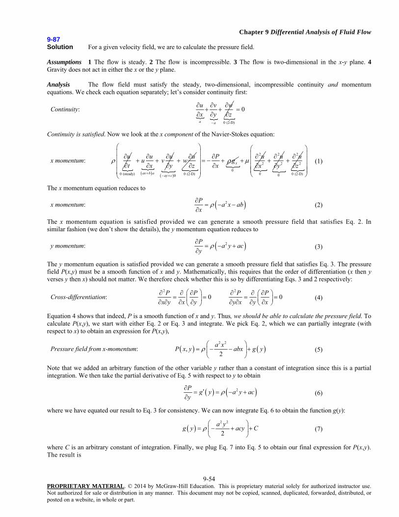
Chapter 9 Differential Analysis of Fluid Flow
9-54 PROPRIETARY MATERIAL. © 2014 by McGraw-Hill Education. This is proprietary material solely for authorized instructor use. Not authorized for sale or distribution in any manner. This document may not be copied, scanned, duplicated, forwarded, distributed, or posted on a website, in whole or part.
9-87 Solution For a given velocity field, we are to calculate the pressure field. Assumptions 1 The flow is steady. 2 The flow is incompressible. 3 The flow is two-dimensional in the x-y plane. 4 Gravity does not act in either the x or the y plane. Analysis The flow field must satisfy the steady, two-dimensional, incompressible continuity and momentum equations. We check each equation separately; let’s consider continuity first:
Continuity:
a a
u v w
x y z
0 (2-D)
0
Continuity is satisfied. Now we look at the x component of the Navier-Stokes equation:
x momentum: u
t
0 (steady) ax b a
u uu v
x y
0ay c
uw
z
0 (2-D)
x
Pg
x
2
2
0
u
x
2
2
0
u
y
2
2
0
u
z
0 (2-D)
(1)
The x momentum equation reduces to
x momentum: 2Pa x ab
x
(2)
The x momentum equation is satisfied provided we can generate a smooth pressure field that satisfies Eq. 2. In similar fashion (we don’t show the details), the y momentum equation reduces to
y momentum: 2Pa y ac
y
(3)
The y momentum equation is satisfied provided we can generate a smooth pressure field that satisfies Eq. 3. The pressure field P(x,y) must be a smooth function of x and y. Mathematically, this requires that the order of differentiation (x then y verses y then x) should not matter. We therefore check whether this is so by differentiating Eqs. 3 and 2 respectively:
Cross-differentiation: 2 2
0 0P P P P
x y x y y x y x
(4)
Equation 4 shows that indeed, P is a smooth function of x and y. Thus, we should be able to calculate the pressure field. To calculate P(x,y), we start with either Eq. 2 or Eq. 3 and integrate. We pick Eq. 2, which we can partially integrate (with respect to x) to obtain an expression for P(x,y),
Pressure field from x-momentum: 2 2
,2
a xP x y abx g y
(5)
Note that we added an arbitrary function of the other variable y rather than a constant of integration since this is a partial integration. We then take the partial derivative of Eq. 5 with respect to y to obtain
2Pg y a y ac
y
(6)
where we have equated our result to Eq. 3 for consistency. We can now integrate Eq. 6 to obtain the function g(y):
2 2
2
a yg y acy C
(7)
where C is an arbitrary constant of integration. Finally, we plug Eq. 7 into Eq. 5 to obtain our final expression for P(x,y). The result is
Chapter 9 Differential Analysis of Fluid Flow
9-55 PROPRIETARY MATERIAL. © 2014 by McGraw-Hill Education. This is proprietary material solely for authorized instructor use. Not authorized for sale or distribution in any manner. This document may not be copied, scanned, duplicated, forwarded, distributed, or posted on a website, in whole or part.
Solution: 2 2 2 2
,2 2
a x a yP x y abx acy C
(8)
Discussion For practice, you should differentiate Eq. 8 with respect to both x and y, and compare to Eqs. 2 and 3. (This also serves as a check of our algebra.) In addition, try to obtain Eq. 8 by starting with Eq. 3 rather than Eq. 2; you should get the same answer. Pressure is found to within some arbitrary constant C since the absolute magnitude of pressure is irrelevant; only pressure gradients are important.

Chapter 9 Differential Analysis of Fluid Flow
9-56 PROPRIETARY MATERIAL. © 2014 by McGraw-Hill Education. This is proprietary material solely for authorized instructor use. Not authorized for sale or distribution in any manner. This document may not be copied, scanned, duplicated, forwarded, distributed, or posted on a website, in whole or part.
9-88 Solution For a given velocity field, we are to calculate the pressure field. Assumptions 1 The flow is steady. 2 The flow is incompressible. 3 The flow is two-dimensional in the x-y plane. 4 Gravity does not act in either the x or the y direction. Analysis The flow field must satisfy the steady, two-dimensional, incompressible continuity and momentum equations. We check each equation separately; let’s consider continuity first:
Continuity:
2 2ax ax
u v w
x y z
0 (2-D)
0
Continuity is satisfied. Now we look at the x component of the Navier-Stokes equation:
x momentum:
u
t
20 (steady) 2ax ax
u uu v
x y
2 0axy
uw
z
0 (2-D)
x
Pg
x
2 2
2 2
02a
u u
x y
2
2
0
u
z
0 (2-D)
(1)
equation 1 reduces to
x momentum: 2 32 2P
a x ax
(2)
The x momentum equation is satisfied provided we can generate a pressure field that satisfies Eq. 2. In similar fashion we examine the y momentum equation,
y momentum:v
t
20 (steady) 2 2 2ax ay axy ax
v v vu v w
x y z
0 (2-D)
y
Pg
y
2
2
0
v
x
2
2
0
v
y
2
2
0
v
z
0 (2-D)
The y momentum equation reduces to
y momentum: 2 22P
a x yy
(3)
The y momentum equation is satisfied provided we can generate a pressure field that satisfies Eq. 3. In the two-dimensional flow under discussion here, the pressure field P(x,y) must be a smooth function of x and y. Mathematically, this requires that the order of differentiation (x then y versus y then x) should not matter. We check whether this is so by differentiating Eqs. 3 and 2 respectively:
Cross-differentiation: 2 2
2 20 2P P P P
a xy x y x x y x y
(4)
Since the cross-derivative terms in Eq. 4 do not match, P is not a smooth function of x and y. Thus, we are unable to calculate a steady, incompressible, two-dimensional pressure field with the given velocity field. We cannot proceed any further. Discussion This problem shows that even if a velocity field satisfies the continuity equation (conservation of mass), and even if we can plot streamlines for the flow field, this does not necessarily guarantee that the velocity field is physically possible. In the present case, for instance, we are unable to find a pressure field that can satisfy the steady Navier-Stokes equation.

Chapter 9 Differential Analysis of Fluid Flow
9-57 PROPRIETARY MATERIAL. © 2014 by McGraw-Hill Education. This is proprietary material solely for authorized instructor use. Not authorized for sale or distribution in any manner. This document may not be copied, scanned, duplicated, forwarded, distributed, or posted on a website, in whole or part.
9-89 Solution For a given velocity field, we are to calculate the pressure field. Assumptions 1 The flow is steady. 2 The flow is incompressible. 3 The flow is two-dimensional in the r- plane. 4 Gravity does not act in either the r or the direction. Analysis The flow must satisfy the steady, two-dimensional, incompressible continuity and momentum equations. We check each equation separately, starting with continuity,
Continuity: 1 rru
r r
0
1 u
r
0
zu
z
0
0
Continuity is satisfied. Now we look at the component of the Navier-Stokes equation,
u
t
2
0 (steady)
r
C K
r r
u u uu
r r
32
0
rz
CKKrr
u u uu
r z
0 (2-D)
1
Pg
r
33
2
2 2 2
0
1 1
KK
rr
u u ur
r r r r r
2
0
2 ru
r
2
2
0
u
z
0 (2-D)
(1)
The momentum equation reduces to
momentum: 0P
(2)
The momentum equation is satisfied provided we can generate a pressure field that satisfies Eq. 2. As a side note, we might have expected Eq. 2 without even working through the algebra, since in this problem the velocity field is independent of angle ; we expect that pressure does not depend on either. In similar fashion the r momentum equation is
ru
t
2
0 (steady)
r rr
C C
r r
uu uu
r r
2
32
2
0
rz
KKrr
u uu
r z
0 (2-D)
r
Pg
r
33
2
2 2 2
0
1 1r r r
CC
rr
u u ur
r r r r r
2
0
2 u
r
2
2
0
ru
z
0 (2-D)
which reduces to
r momentum: 2 2
3
P K C
r r
(3)
The r momentum equation is satisfied provided we can generate a pressure field that satisfies Eq. 3. The pressure field P(r,) must be a smooth function of r and . Mathematically, this requires that the order of differentiation (r then versus then r) should not matter. We therefore check whether this is so by differentiating Eqs. 2 and 3 respectively:

Chapter 9 Differential Analysis of Fluid Flow
9-58 PROPRIETARY MATERIAL. © 2014 by McGraw-Hill Education. This is proprietary material solely for authorized instructor use. Not authorized for sale or distribution in any manner. This document may not be copied, scanned, duplicated, forwarded, distributed, or posted on a website, in whole or part.
Cross-differentiation: 2 2
0 0P P P P
r r r r
(4)
Equation 4 shows that indeed, P is a smooth function of r and . Thus, we should be able to calculate the pressure field. To calculate P(r,), we start with either Eq. 2 or Eq. 3 and integrate. We pick Eq. 2, which we can partially integrate (with respect to ) to obtain an expression for P(r,),
Pressure field from -momentum: , 0P r g r (5)
Note that we added an arbitrary function of the other variable r rather than a constant of integration since this is a partial integration. We then take the partial derivative of Eq. 5 with respect to r to obtain
2 2
3
P K Cg r
r r
(6)
where we have equated our result to Eq. 3 for consistency. We can now integrate Eq. 6 to obtain the function g(r):
2 2
12
1
2
K Cg r C
r
(7)
where C1 is an arbitrary constant of integration. Finally, we plug Eq. 7 into Eq. 5 to obtain our final expression for P(x,y). The result is
Answer: 2 2
12
1,
2
K CP r C
r
(8)
Thus the pressure field for this flow decreases like 1/r2 as we approach the origin. (The origin itself is a singularity point.) This flow field is a simplistic model of a tornado or hurricane, and the low pressure at the center is the “eye of the storm”. We note that this flow field is irrotational, and thus Bernoulli’s equation can be used instead to calculate the pressure. If we call the pressure P far away from the origin (r ), where the local velocity approaches zero, Bernoulli’s equation shows that at any distance r from the origin,
Bernoulli equation: 2 2
22
1 1
2 2
K CP V P P P
r
(9)
Equation 9 agrees with our solution (Eq. 8) from the full Navier-Stokes equation if we set constant C1 equal to P. A region of rotational flow near the origin would avoid the singularity there, and would yield a more physically realistic model of a real tornado. Discussion For practice, try to obtain Eq. 8 by starting with Eq. 3 rather than Eq. 2; you should get the same answer.

Chapter 9 Differential Analysis of Fluid Flow
9-59 PROPRIETARY MATERIAL. © 2014 by McGraw-Hill Education. This is proprietary material solely for authorized instructor use. Not authorized for sale or distribution in any manner. This document may not be copied, scanned, duplicated, forwarded, distributed, or posted on a website, in whole or part.
9-90 Solution For a given velocity field, we are to calculate the pressure field. Assumptions 1 The flow is steady. 2 The flow is incompressible. 3 The flow is two-dimensional in the x-y plane. 4 Gravity does not act in either the x or the y direction. Analysis The flow field must satisfy the steady, two-dimensional, incompressible continuity and momentum equations. We check each equation separately; let’s consider continuity first:
Continuity:
a a
u v w
x y z
0 (2-D)
0
Continuity is satisfied. Now we look at the x component of the Navier-Stokes equation:
x momentum:
u
t
0 (steady) ax b a
u uu v
x y
2 0ay cx
uw
z
0 (2-D)
x
Pg
x
2
2
0
u
x
2
2
0
u
y
2
2
0
u
z
0 (2-D)
(1)
Equation 1 reduces to
x momentum: 2Pa x ab
x
(2)
The x momentum equation is satisfied provided we can generate a pressure field that satisfies Eq. 2. In similar fashion we examine the y momentum equation,
y momentum:v
t
220 (steady) ax b cxay cx a
v v vu v w
x y z
0 (2-D)
y
Pg
y
2 2
2 2
0 2c
v v
x y
2
2
0
v
z
0 (2-D)
The y momentum equation reduces to
y momentum: 2 22 2P
acx bcx a y cy
(3)
The y momentum equation is satisfied provided we can generate a pressure field that satisfies Eq. 3. In the two-dimensional flow under discussion here, the pressure field P(x,y) must be a smooth function of x and y. Mathematically, this requires that the order of differentiation (x then y versus y then x) should not matter. We check whether this is so by differentiating Eqs. 3 and 2 respectively:
Cross-differentiation: 2 2
0 2 2P P P P
acx bcy x y x x y x y
(4)
Since the cross-derivative terms in Eq. 4 do not match, P is not a smooth function of x and y. Thus, we are unable to calculate a steady, incompressible, two-dimensional pressure field with the given velocity field. We cannot proceed any farther – the pressure cannot be found with the given velocity field and restrictions. Discussion This problem shows that if a velocity field satisfies the continuity equation (conservation of mass), this does not necessarily guarantee that the velocity field is physically possible. In the present case, for instance, we are unable to find a pressure field that can satisfy the steady form of the Navier-Stokes equation.

Chapter 9 Differential Analysis of Fluid Flow
9-60 PROPRIETARY MATERIAL. © 2014 by McGraw-Hill Education. This is proprietary material solely for authorized instructor use. Not authorized for sale or distribution in any manner. This document may not be copied, scanned, duplicated, forwarded, distributed, or posted on a website, in whole or part.
9-91 Solution For a given geometry and set of boundary conditions, we are to calculate the velocity field, and plot the nondimensionalized velocity profile. Assumptions We number and list the assumptions for clarity:
1 The walls are infinite in the y-z plane (y is into the page). 2 The flow is steady, i.e. time derivatives of any quantity are zero. 3 The flow is parallel (the x component of velocity, u, is zero everywhere). 4 The fluid is incompressible and Newtonian, and the flow is laminar. 5 Pressure P = constant everywhere. In other words, there is no applied pressure gradient pushing the flow; the flow
establishes itself due to a balance between gravitational forces and viscous forces. 6 The velocity field is purely two-dimensional, which implies that v = 0 and all y derivatives are zero.
7 Gravity acts in the negative z direction. We can express this mathematically as g gk
, or gx = gy = 0 and gz =
g. Analysis We obtain the velocity and pressure fields by following the step-by-step procedure for differential fluid flow solutions.
Step 1 Set up the problem and the geometry. See problem statement. Step 2 List assumptions and boundary conditions. We have already listed seven assumptions. The boundary conditions
come from the no-slip condition at the walls (1) at x = h/2, u = v = w = 0. (2) At x = h/2, u = v = w = 0. Step 3 Write out and simplify the differential equations. We start with the continuity equation in Cartesian coordinates,
Continuity: u
x
Assumption 3
v
y
Assumption 6
0 or 0w w
z z
(1)
Equation 1 tells us that w is not a function of z. In other words, it doesn’t matter where we place our origin – the flow is the same at any z location. In other words the flow is fully developed. Since w is not a function of time (Assumption 2), z (Eq. 1), or y (Assumption 6), we conclude that w is at most a function of x,
Result of continuity: onlyw w x (2)
We now simplify each component of the Navier-Stokes equation as far as possible. Since u = v = 0 everywhere and gravity does not act in the x or y directions, the x and y momentum equations are satisfied exactly (in fact all terms are zero in both equations). The z momentum equation reduces to
z momentum:
w
t
Assumption 2
wu
x
Assumption 3
wv
y
Assumption 6
ww
z
Continuity
P
z
Assumption 5
2 2
2 2
z
g
g
w w
x y
2
2
Assumption 6
w
z
2
2
continuity
or d w g
dx
(3)
We have changed from a partial derivative (/x) to a total derivative (d/dx) in Eq. 3 as a direct result of Eq. 2, reducing the PDE to an ODE.
Step 4 Solve the differential equations. Continuity and x and y momentum have already been “solved”. Equation 3 (z momentum) is integrated twice to get
Integration of z momentum: 21 22
gw x C x C
(4)
Step 5 We apply boundary conditions (1) and (2) from Step 2 above to obtain constants C1 and C2,

Chapter 9 Differential Analysis of Fluid Flow
9-61 PROPRIETARY MATERIAL. © 2014 by McGraw-Hill Education. This is proprietary material solely for authorized instructor use. Not authorized for sale or distribution in any manner. This document may not be copied, scanned, duplicated, forwarded, distributed, or posted on a website, in whole or part.
Boundary condition (1): 21 20
8 2
g hh C C
and
Boundary condition (2): 21 20
8 2
g hh C C
We solve the above two equations simultaneously to obtain expressions for C1 and C2,
Constants of integration: 21 20
8
gC C h
Finally, Eq. 4 becomes
Final result for velocity field: 2
2
2 2
g hw x
(5)
Since h/2 < x < h/2 everywhere, w is negative everywhere as expected (flow is downward).
Step 6 Verify the results. You can plug in the velocity field to verify that all the differential equations and boundary conditions are satisfied.
We nondimensionalize Eq. 5 by inspection: we let x* = x/h and w* = w/(gh2). Eq. 5 becomes
Nondimensionalized velocity profile: 21 1* *
2 4w x
(6)
We plot the nondimensional velocity field in Fig. 1. The velocity profile is parabolic. Discussion Equation 4 for the z component of velocity is identical to that of Example 9-17. In fact, the present problem is identical to Example 9-17 except for the boundary conditions and the location of the origin. Comparing the two results, we see that the maximum nondimensional velocity for the case with two walls is one-fourth than that for the case with only one wall. This is not unexpected – the additional wall leads to more viscous forces that retard the flow.
-0.14
-0.12
-0.1
-0.08
-0.06
-0.04
-0.02
0
-0.5 -0.3 -0.1 0.1 0.3 0.5x*
w*
FIGURE 1 The velocity profile for liquid falling between two vertical walls.

Chapter 9 Differential Analysis of Fluid Flow
9-62 PROPRIETARY MATERIAL. © 2014 by McGraw-Hill Education. This is proprietary material solely for authorized instructor use. Not authorized for sale or distribution in any manner. This document may not be copied, scanned, duplicated, forwarded, distributed, or posted on a website, in whole or part.
9-92 Solution We are to calculate and compare the volume flow rate per unit width of fluid falling between two vertical walls and fluid falling along one vertical wall. Assumptions 1 The flow is steady. 2 The flow is incompressible. 3 The walls are infinitely wide and very long so that all of the parallel flow, fully developed approximations of the previous problem hold. Analysis We calculate the volume flow rate per unit width by integration of the velocity:
Volume flow rate per unit depth, two vertical walls:
/ 22 3 2 3 3 3 3 3/ 2 / 2 2
/ 2 / 2/ 2
2 2 2 3 4 2 24 8 24 8 12
x hh h
h hx h
g h g x h g h h h h ghwdx x dx x
L
V (1)
The result is negative since we have defined positive volume flow rate upward, since z is upward, but the flow is downward. For the case with only one vertical wall and a free surface, we calculate the vertical component of velocity to be
22
gxw x h
(see Example 9-17). Thus, we calculate / LV for the case of one vertical wall to be
Volume flow rate per unit depth, one vertical wall with a free surface:
3 3 3
2 3
0 00
2 0 02 2 3 2 3 3
x hh h
x
gx g x g h ghwdx x h dx x h h
L
V
(2)
Comparing the two cases we see that / LV for the case of one vertical wall and a free surface is four times greater than the case of two vertical walls with no free surface. The physical explanation is that with two walls, the fluid is held back by more viscous stresses, leading to a parabolic velocity profile. For the single-wall case the free surface has no shear stress and thus the fluid flows more freely. Discussion The two flows being compared here are identical except for the boundary conditions. This illustrates the importance of setting proper boundary conditions.

Chapter 9 Differential Analysis of Fluid Flow
9-63 PROPRIETARY MATERIAL. © 2014 by McGraw-Hill Education. This is proprietary material solely for authorized instructor use. Not authorized for sale or distribution in any manner. This document may not be copied, scanned, duplicated, forwarded, distributed, or posted on a website, in whole or part.
9-93 Solution For a given geometry and set of boundary conditions, we are to calculate the velocity and pressure fields, and plot the nondimensional velocity profile.
Assumptions We number and list the assumptions for clarity: 1 The wall is infinite in the s-y plane (y is out of the page for a right-handed coordinate system).
2 The flow is steady, i.e. anything 0t
.
3 The flow is parallel and fully developed (we assume the normal component of velocity, un, is zero, and we assume that the streamwise component of velocity us is independent of streamwise coordinate s).
4 The fluid is incompressible and Newtonian, and the flow is laminar. 5 Pressure P = constant = Patm at the free surface. In other words, there is no applied pressure gradient pushing the
flow; the flow establishes itself due to a balance between gravitational forces and viscous forces along the wall. Atmospheric pressure is constant everywhere since we are neglecting the change of air pressure with elevation.
6 The velocity field is purely two-dimensional, which implies that v = 0 and y
(any velocity component) = 0.
7 Gravity acts in the negative z direction. We can express this mathematically as g gk
. In the s-n plane, gs =
gsin and gn = gcos.
Analysis We obtain the velocity and pressure fields by following the step-by-step procedure for differential fluid flow solutions.
Step 1 Set up the problem and the geometry. See Problem statement. Step 2 List assumptions and boundary conditions. We have already listed seven assumptions. The boundary conditions
are (1) No slip at the wall: at n = 0, us = v = un = 0. (2) At the free surface (n = h) there is no shear, which in this coordinate system at the vertical free surface means us/n = 0. (3) P = Patm at n = h.
Step 3 Write out and simplify the differential equations. We start with the continuity equation in modified Cartesian coordinates, (s,y,n) and (us,v,un),
Continuity: su v
s y
Assumption 6
nu
n
Assumption 3
0 or 0su
s
(1)
Equation 1 tells us that us is not a function of s. In other words, it doesn’t matter where we place our origin – the flow is the same at any s location. This does not tell us anything new; we have already assumed that the flow is fully developed (Assumption 3). Furthermore, since us is not a function of time (Assumption 2) or y (Assumption 6), we conclude that us is at most a function of n,
Result of continuity: onlys su u n (2)
We now simplify each component of the Navier-Stokes equation as far as possible. Since v = 0 everywhere and gravity does not act in the y direction, the y momentum equation is satisfied exactly (in fact all terms are zero). Since un = 0 everywhere, the only non-zero terms in the n momentum equation are the pressure term and the gravity term. The n momentum equation reduces to
n momentum:
nDu
Dt
2
cosAssumption 3
n n
g
Pg u
n
Assumption 3
or cosP
gn
(3)
We integrate Eq. 3 to solve for the pressure,
Pressure: cosP gn f s (4)
where we have added a function of s rather than a simple constant of integration. But from boundary condition (3), at n = h, P = Patm. Thus Eq. 4 yields atm cosf s P gh . In other words, f(s) is really not a function of s at all.
Equation 4 then becomes
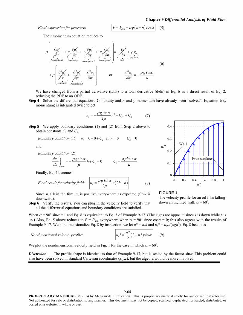
Chapter 9 Differential Analysis of Fluid Flow
9-64 PROPRIETARY MATERIAL. © 2014 by McGraw-Hill Education. This is proprietary material solely for authorized instructor use. Not authorized for sale or distribution in any manner. This document may not be copied, scanned, duplicated, forwarded, distributed, or posted on a website, in whole or part.
Final expression for pressure: atm cosP P g h n (5)
The s momentum equation reduces to
su
t
Assumption 2
ss
uu
s
Continuity
suv
y
Assumption 6
sn
uu
n
Assumption 3
P
s
sinEq. 5
2
2
s
g
s
g
u
s
2
2
continuity
su
y
2 2
2 2
Assumption 6
sin or s su d u g
n dn
(6)
We have changed from a partial derivative (/n) to a total derivative (d/dn) in Eq. 6 as a direct result of Eq. 2, reducing the PDE to an ODE.
Step 4 Solve the differential equations. Continuity and n and y momentum have already been “solved”. Equation 6 (s momentum) is integrated twice to get
21 2
sin
2s
gu n C n C
(7)
Step 5 We apply boundary conditions (1) and (2) from Step 2 above to obtain constants C1 and C2,
Boundary condition (1): 2 20 0 at 0 0su C n C
and
Boundary condition (2):
1 1
sin sin0 s
n h
du g ghh C C
dn
Finally, Eq. 4 becomes
Final result for velocity field: sin2
2s
gu n h n
(8)
Since n < h in the film, us is positive everywhere as expected (flow is downward).
Step 6 Verify the results. You can plug in the velocity field to verify that all the differential equations and boundary conditions are satisfied.
When = 90o sin = 1 and Eq. 8 is equivalent to Eq. 5 of Example 9-17. (The signs are opposite since s is down while z is up.) Also, Eq. 5 above reduces to P = Patm everywhere when = 90o since cos = 0; this also agrees with the results of Example 9-17. We nondimensionalize Eq. 8 by inspection: we let n* = n/h and us* = us/(gh2). Eq. 8 becomes
Nondimensional velocity profile: ** 2 * sin
2s
nu n (9)
We plot the nondimensional velocity field in Fig. 1 for the case in which = 60o.
Discussion The profile shape is identical to that of Example 9-17, but is scaled by the factor sin. This problem could also have been solved in standard Cartesian coordinates (x,y,z), but the algebra would be more involved.
0
0.1
0.2
0.3
0.4
0 0.2 0.4 0.6 0.8 1n*
us*Wall
Free surface
FIGURE 1 The velocity profile for an oil film falling down an inclined wall, = 60o.

Chapter 9 Differential Analysis of Fluid Flow
9-65 PROPRIETARY MATERIAL. © 2014 by McGraw-Hill Education. This is proprietary material solely for authorized instructor use. Not authorized for sale or distribution in any manner. This document may not be copied, scanned, duplicated, forwarded, distributed, or posted on a website, in whole or part.
9-94 Solution We are to calculate the volume flow rate per unit width of oil falling down a vertical wall. Assumptions 1 The flow is steady. 2 The flow is incompressible. 3 The wall is infinitely wide and very long so that all of the parallel flow, fully developed approximations of Problem 9-89 hold. Analysis We calculate the volume flow rate per unit width by integration of the velocity:
Volume flow rate per unit depth: 3
0 0
sin sin2
2 3
h h
s
g gu dn n h n dn h
V
L
(1)
For an oil film of thickness 5.0 mm with = 888 kg/m3 and = 0.80 kg/(ms), we calculate V / L using Eq. 1,
Result:
33 2 o
3888 kg/m 9.81 m/s sin 60 0.005 msin
3 3 0.80 kg/m s
gh
L
-4 23.93×10 m /sV
Discussion Since viscosity is in the denominator of Eq. 1, a low viscosity liquid (like water) would yield a larger volume flow rate; this agrees with our intuition. Likewise, a larger density liquid and/or a thicker film would yield a larger volume flow rate, again agreeing with our intuition. Finally, if = 0o there is no flow.
9-95 Solution We are to expand two terms into three terms, and then compress the three terms into one term. Analysis We use the product rule to differentiate the expression,
2
2 2 2
1 1u u u u ur
r r r r rr r r
The second part of this question involves some trial and error, using the product rule in reverse. After some effort we get
2
2 2
1 1u u uru
r r r r rr r
(1)
You can apply the product rule to verify Eq. 1. Discussion The grouping of these terms into one term as in Eq. 1 turns out to be useful for some analytical solutions of the Navier-Stokes equation.

Chapter 9 Differential Analysis of Fluid Flow
9-66 PROPRIETARY MATERIAL. © 2014 by McGraw-Hill Education. This is proprietary material solely for authorized instructor use. Not authorized for sale or distribution in any manner. This document may not be copied, scanned, duplicated, forwarded, distributed, or posted on a website, in whole or part.
9-96 Solution For a given geometry and set of boundary conditions, we are to calculate the velocity field. Assumptions We number and list the assumptions for clarity:
1 The cylinders are infinite in the z direction (z is out of the page in the figure of the problem statement for a right-handed coordinate system). The velocity field is purely two-dimensional, which implies that w = 0 and derivatives of any velocity component with respect to z are zero.
2 The flow is steady, meaning that all time derivatives are zero. 3 The flow is circular, meaning that the radial velocity component ur is zero. 4 The flow is rotationally symmetric, meaning that nothing is a function of . 5 The fluid is incompressible and Newtonian, and the flow is laminar. 6 Gravitational effects are ignored. (Note that gravity may act in the z direction, leading to an additional hydrostatic
pressure distribution in the z direction. This would not affect the present analysis.) Analysis We obtain the velocity and pressure fields by following the step-by-step procedure for differential fluid flow solutions.
Step 1 Set up the problem and the geometry. See the problem statement. Step 2 List assumptions and boundary conditions. We have already listed five assumptions. The boundary conditions are
(1) No slip at the inner wall: at r = Ri, u = iRi. (2) No slip at the outer wall: at r = Ro, u = 0. Step 3 Write out and simplify the differential equations. We start with the continuity equation in cylindrical coordinates,
(r,,z) and (ur,u,uz),
Continuity: 1 rru
r r
Assumption 3
1 u
r
Assumption 4
w
z
Assumption 1
0 or 0 0 (1)
Thus continuity is satisfied exactly by our assumptions. We now simplify each component of the Navier-Stokes equation as far as possible. Since w = 0 everywhere and gravity is ignored, the z momentum equation is satisfied exactly (in fact all terms are zero). Since ur = 0 everywhere, the only non-zero terms in the r momentum equation are the pressure term and the “extra” term that involves u. The r momentum equation reduces to
r momentum: 2 2
or u uP dP
r r dr r
(2)
We have changed the partial derivatives to total derivatives since P is a function only of r. Equation 2 could be used to solve for P(r) once we find u. The momentum equation is written out, using the result of the previous problem,
momentum:
u
t
Assumption 2
r
uu
r
Assumption 3
u u
r
Assumption 4
ru u
r
Assumption 3
z
uu
z
Assumption 1
1
P
r
Assumption 4
g
2
2 2
Assumption 6
1 1 uru
r r r r
2
Assumption 4
2 ru
r
2
2
Assumption 3
u
z
Assumption 6
Again we change from partial derivatives (/r) to a total derivatives (d/dr), reducing the PDE to an ODE. The momentum equation reduces to
Reduced momentum: 10
d dru
dr r dr
(3)
Step 4 Solve the differential equations. Continuity and z momentum have already been “solved”. Equation 3 ( momentum) is integrated once,

Chapter 9 Differential Analysis of Fluid Flow
9-67 PROPRIETARY MATERIAL. © 2014 by McGraw-Hill Education. This is proprietary material solely for authorized instructor use. Not authorized for sale or distribution in any manner. This document may not be copied, scanned, duplicated, forwarded, distributed, or posted on a website, in whole or part.
Integration of momentum: 1
1 dru C
r dr
After multiplying by r we integrate again. After division by r we get
u: 21 2
Cru C
r (4)
Step 5 We apply boundary conditions (1) and (2) from Step 2 above to obtain constants C1 and C2,
Boundary condition (2): 2
21 2 10 or
2 2o o
o
R RCC C C
R
and
Boundary condition (1): 2
21 1 12 2 2
i i oi i
i i
R R RCR C C C
R R
Which can be solved for C1. The two constants of integration are thus
Constants of integration: 2 2 2
1 22 2 2 2
2 i i o i i
o i o i
R R RC C
R R R R
Finally, Eq. 4 becomes (after a bit of algebra)
Final result for velocity field: 2 2
2 2i i o
o i
R Ru r
rR R
(5)
Step 6 Verify the results. You can plug in the velocity field to verify that all the differential equations and boundary conditions are satisfied.
Discussion There are valid alternative forms of Eq. 5. We could integrate Eq. 2 to solve for the pressure since we now know u from Eq. 5. The algebra is laborious, but not difficult.

Chapter 9 Differential Analysis of Fluid Flow
9-68 PROPRIETARY MATERIAL. © 2014 by McGraw-Hill Education. This is proprietary material solely for authorized instructor use. Not authorized for sale or distribution in any manner. This document may not be copied, scanned, duplicated, forwarded, distributed, or posted on a website, in whole or part.
9-97 Solution For a given geometry and set of boundary conditions, we are to calculate the velocity field. Assumptions We number and list the assumptions for clarity:
1 The cylinders are infinite in the z direction (z is out of the page in the figure of the problem statement for a right-handed coordinate system). The velocity field is purely two-dimensional, which implies that w = 0 and derivatives of any velocity component with respect to z are zero.
2 The flow is steady, meaning that all time derivatives are zero. 3 The flow is circular, meaning that the radial velocity component ur is zero. 4 The flow is rotationally symmetric, meaning that nothing is a function of . 5 The fluid is incompressible and Newtonian, and the flow is laminar. 6 Gravitational effects are ignored. (Note that gravity may act in the z direction, leading to an additional hydrostatic
pressure distribution in the z direction. This would not affect the present analysis.) Analysis We obtain the velocity and pressure fields by following the step-by-step procedure for differential fluid flow solutions.
Step 1 Set up the problem and the geometry. See the problem statement. Step 2 List assumptions and boundary conditions. We have already listed five assumptions. The boundary conditions are
(1) No slip at the inner wall: at r = Ri, u = 0. (2) No slip at the outer wall: at r = Ro, u = oRo. Step 3 Write out and simplify the differential equations. We start with the continuity equation in cylindrical coordinates,
(r,,z) and (ur,u,uz),
Continuity: 1 rru
r r
Assumption 3
1 u
r
Assumption 4
w
z
Assumption 1
0 or 0 0 (1)
Thus continuity is satisfied exactly by our assumptions. We now simplify each component of the Navier-Stokes equation as far as possible. Since w = 0 everywhere and gravity is ignored, the z momentum equation is satisfied exactly (in fact all terms are zero). Since ur = 0 everywhere, the only non-zero terms in the r momentum equation are the pressure term and the “extra” term that involves u. The r momentum equation reduces to
r momentum: 2 2
or u uP dP
r r dr r
(2)
We have changed the partial derivatives to total derivatives since P is a function only of r. Equation 2 could be used to solve for P(r) once we find u. The momentum equation is written out, using the result of the previous problem,
momentum:
u
t
Assumption 2
r
uu
r
Assumption 3
u u
r
Assumption 4
ru u
r
Assumption 3
z
uu
z
Assumption 1
1
P
r
Assumption 4
g
2
2 2
Assumption 6
1 1 uru
r r r r
2
Assumption 4
2 ru
r
2
2
Assumption 3
u
z
Assumption 6
Again we change from partial derivatives (/r) to a total derivatives (d/dr), reducing the PDE to an ODE. The momentum equation reduces to
Reduced momentum: 10
d dru
dr r dr
(3)
Step 4 Solve the differential equations. Continuity and z momentum have already been “solved”. Equation 3 ( momentum) is integrated once,

Chapter 9 Differential Analysis of Fluid Flow
9-69 PROPRIETARY MATERIAL. © 2014 by McGraw-Hill Education. This is proprietary material solely for authorized instructor use. Not authorized for sale or distribution in any manner. This document may not be copied, scanned, duplicated, forwarded, distributed, or posted on a website, in whole or part.
Integration of momentum: 1
1 dru C
r dr
After multiplying by r we integrate again. After division by r we get
u: 21 2
Cru C
r (4)
Step 5 We apply boundary conditions (1) and (2) from Step 2 above to obtain constants C1 and C2,
Boundary condition (1): 2
21 2 10 or
2 2i i
i
R RCC C C
R
and
Boundary condition (2): 2
21 1 12 2 2
o o io o
o o
R R RCR C C C
R R
Which can be solved for C1. The two constants of integration are thus
Constants of integration: 2 2 2
1 22 2 2 2
2 o o o i o
o i o i
R R RC C
R R R R
Finally, Eq. 4 becomes (after a bit of algebra)
Final result for velocity field: 2 2
2 2o o i
o i
R Ru r
rR R
(5)
Step 6 Verify the results. You can plug in the velocity field to verify that all the differential equations and boundary conditions are satisfied.
Discussion There are valid alternative forms of Eq. 5. We could integrate Eq. 2 to solve for the pressure since we now know u from Eq. 5. The algebra is laborious, but not difficult.
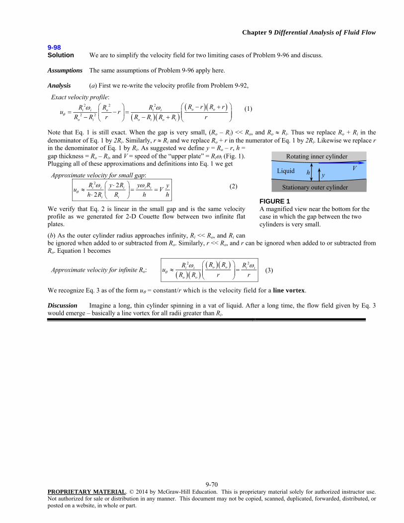
Chapter 9 Differential Analysis of Fluid Flow
9-70 PROPRIETARY MATERIAL. © 2014 by McGraw-Hill Education. This is proprietary material solely for authorized instructor use. Not authorized for sale or distribution in any manner. This document may not be copied, scanned, duplicated, forwarded, distributed, or posted on a website, in whole or part.
9-98 Solution We are to simplify the velocity field for two limiting cases of Problem 9-96 and discuss. Assumptions The same assumptions of Problem 9-96 apply here. Analysis (a) First we re-write the velocity profile from Problem 9-92,
Exact velocity profile:
2 2 2
2 2
o oi i o i i
o i o io i
R r R rR R Ru r
r R R R R rR R
(1)
Note that Eq. 1 is still exact. When the gap is very small, (Ro – Ri) << Ro, and Ro Ri. Thus we replace Ro + Ri in the denominator of Eq. 1 by 2Ri. Similarly, r Ri and we replace Ro + r in the numerator of Eq. 1 by 2Ri. Likewise we replace r in the denominator of Eq. 1 by Ri. As suggested we define y = Ro – r, h = gap thickness = Ro – Ri, and V = speed of the “upper plate” = Rii (Fig. 1). Plugging all of these approximations and definitions into Eq. 1 we get
Approximate velocity for small gap:
2 2
2i i i i i
i i
R y R y R yu V
h R R h h
(2)
We verify that Eq. 2 is linear in the small gap and is the same velocity profile as we generated for 2-D Couette flow between two infinite flat plates.
(b) As the outer cylinder radius approaches infinity, Ri << Ro, and Ri can be ignored when added to or subtracted from Ro. Similarly, r << Ro, and r can be ignored when added to or subtracted from Ro. Equation 1 becomes
Approximate velocity for infinite Ro: 2 2
o oi i i i
o o
R RR Ru
R R r r
(3)
We recognize Eq. 3 as of the form u = constant/r which is the velocity field for a line vortex. Discussion Imagine a long, thin cylinder spinning in a vat of liquid. After a long time, the flow field given by Eq. 3 would emerge – basically a line vortex for all radii greater than Ri.
V y h Liquid
Rotating inner cylinder
Stationary outer cylinder
FIGURE 1 A magnified view near the bottom for the case in which the gap between the two cylinders is very small.

Chapter 9 Differential Analysis of Fluid Flow
9-71 PROPRIETARY MATERIAL. © 2014 by McGraw-Hill Education. This is proprietary material solely for authorized instructor use. Not authorized for sale or distribution in any manner. This document may not be copied, scanned, duplicated, forwarded, distributed, or posted on a website, in whole or part.
9-99 Solution For a given geometry and set of boundary conditions, we are to calculate the velocity field.
Assumptions The assumptions are identical to those of Problem 9-96.
Analysis We obtain the velocity and pressure fields by following the step-by-step procedure for differential fluid flow solutions. Everything is identical to Problem 9-96 except for the boundary condition at the outer cylinder wall. We re-write boundary condition (2): at r = Ro, u = oRo. We will not repeat all the algebra associated with the equations of motion. The tangential velocity component is still
u: 21 2
Cru C
r (1)
Now we apply boundary conditions (1) and (2) to obtain constants C1 and C2,
Boundary condition (1): 1 2
1
2i
i ii
RC C R
R (2)
Boundary condition (2): 1 2
1
2o
o oo
RC C R
R (3)
We solve Eqs. 2 and 3 simultaneously for C1 and C2. The result is
Constants of integration: 2 2 2 2
1 22 2 2 2
2
o o i i o i i o
o i o i
R R R RC C
R R R R
(4)
Finally, Eq. 4 becomes (after a bit of algebra)
Final result for velocity field: 2 22 2
2 2
1 o i i oo o i i
o i
R Ru R R r
rR R
(5)
We set o = 0 in Eq. 5 to verify that it simplifies to the result of Problem 9-92,
Simplified velocity field: 2 2
2 2i i o
o i
R Ru r
rR R
(6)
Discussion There are valid alternative forms of Eq. 5.

Chapter 9 Differential Analysis of Fluid Flow
9-72 PROPRIETARY MATERIAL. © 2014 by McGraw-Hill Education. This is proprietary material solely for authorized instructor use. Not authorized for sale or distribution in any manner. This document may not be copied, scanned, duplicated, forwarded, distributed, or posted on a website, in whole or part.
9-100 Solution We are to discuss a simplified version of the velocity field of the previous problem.
Assumptions The assumptions are identical to those of the previous problem.
Analysis We set Ri = i = 0 in Eq. 5 of the previous problem. The tangential velocity component simplifies to
Simplified u: 2
2
1o o o
o
u R r rR (1)
We recognize Eq. 1 as the velocity field for solid body rotation. To set up this velocity field in a physical experiment, we would place a cylindrical container of liquid on a rotating table. After a long time, the entire tank, including the liquid, would be in solid body rotation.
Discussion If you imagine flow between the inner and outer cylinders, and then imagine that the inner cylinder stops spinning and shrinks to infinitesimal radius, you can convince yourself that solid body rotation would result.

Chapter 9 Differential Analysis of Fluid Flow
9-73 PROPRIETARY MATERIAL. © 2014 by McGraw-Hill Education. This is proprietary material solely for authorized instructor use. Not authorized for sale or distribution in any manner. This document may not be copied, scanned, duplicated, forwarded, distributed, or posted on a website, in whole or part.
9-101 Solution For flow in a pipe annulus we are to calculate the velocity field. Assumptions We number and list the assumptions for clarity:
1 The pipe is infinitely long in the x direction.
2 The flow is steady, i.e. anything 0t
.
3 This is a parallel flow (the r component of velocity, ur, is zero). 4 The fluid is incompressible and Newtonian, and the flow is laminar. 5 A constant pressure gradient is applied in the x direction such that pressure changes linearly with respect to x
according to the given expression. 6 The velocity field is axisymmetric with no swirl, implying that u = 0 and
anything 0
.
7 We ignore the effects of gravity. Analysis We obtain the velocity field by following the step-by-step procedure for differential fluid flow solutions.
Step 1 Lay out the problem and the geometry. See the problem statement. Step 2 List assumptions and boundary conditions. We have already listed seven assumptions. The boundary conditions
come from imposing the no slip condition at both pipe walls: (1) at r = Ri, 0V
. (2) at r = Ro, 0V
. Step 3 Write out and simplify the differential equations. We start with the continuity equation in cylindrical coordinates,
Continuity: 1 rru
r r
Assumption 3
1 u
r
Assumption 6
0 or 0u u
x x
(1)
Equation 1 tells us that u is not a function of x. In other words, it doesn’t matter where we place our origin – the flow is the same at any x location. This can also be inferred directly from Assumption 1, which tells us that there is nothing special about any x location since the pipe is infinite in length – the flow is fully developed. Furthermore, since u is not a function of time (Assumption 2) or (Assumption 6), we conclude that u is at most a function of r,
Result of continuity: onlyu u r (2)
Next we simplify the x momentum equation as far as possible:
x momentum:
u
t
Assumption 2
r
uu
r
Assumption 3
u u
r
Assumption 6
uu
x
Continuity
x
Pg
x
2
2 2
Assumption 7
1 1u ur
r r r r
2
2
Assumption 6
u
x
Continuity
(3)
or
Result of x momentum: 1 1d du P
rr dr dr x
(4)
Note that we have replaced the partial derivative operators for the u derivatives with total derivative operators because of Eq. 2. Every term in the r momentum equation is zero except the pressure gradient term, forcing that lone term to also be zero,
r momentum: 0P
r
(5)

Chapter 9 Differential Analysis of Fluid Flow
9-74 PROPRIETARY MATERIAL. © 2014 by McGraw-Hill Education. This is proprietary material solely for authorized instructor use. Not authorized for sale or distribution in any manner. This document may not be copied, scanned, duplicated, forwarded, distributed, or posted on a website, in whole or part.
In other words, P is not a function of r. Since P is also not a function of time (Assumption 2) or (Assumption 6), P can be at most a function of x,
Result of r momentum: onlyP P x (6)
Therefore we can replace the partial derivative operator for the pressure gradient in Eq. 4 by the total derivative operator since P varies only with x. Finally, all terms of the component of the Navier-Stokes equation go to zero.
Step 4 Solve the differential equations. Continuity and r momentum have already been “solved”, resulting in Eqs. 2 and 6 respectively. The momentum equation has vanished, and thus we are left with Eq. 4 (x momentum). After multiplying both sides by r, we integrate once to obtain
Integration of x momentum: 2
12
du r dPr C
dr dx
(7)
where C1 is a constant of integration. Note that the pressure gradient dP/dx is a constant here. After dividing both sides of Eq. 7 by r, we can integrate a second time to get
Second integration of x momentum: 2
1 2ln4
r dPu C r C
dx
(8)
where C2 is a second constant of integration. Step 5 Apply boundary conditions from Step 2 above to obtain constants C1 and C2:
Boundary condition (1): 2
1 20 ln4
ii
R dPC R C
dx
Boundary condition (2): 2
1 20 ln4
oo
R dPC R C
dx
We solve the above two equations simultaneously to find C1 and C2,
Constants: 2 2 2 2
1 2
ln ln
4 ln 4 ln
o i o i i o
o o
i i
R R R R R RdP dPC C
R Rdx dxR R
After some algebra and rearrangement, Eq. 7 becomes
Final result for axial velocity:
2 2
2
ln ln1
4 ln
i oo i
o
i
r rR R
R RdPu r
RdxR
(9)
Step 6 Verify the results. You can plug in the velocity field to verify that all the differential equations and boundary conditions are satisfied.
Discussion There are other valid forms of Eq. 9. For example, after some rearrangement, Eq. 9 can be written as
Alternative form: 2 2
221ln
4 ln
o io
o o
i
R RdP ru r R
Rdx RR
(10)

Chapter 9 Differential Analysis of Fluid Flow
9-75 PROPRIETARY MATERIAL. © 2014 by McGraw-Hill Education. This is proprietary material solely for authorized instructor use. Not authorized for sale or distribution in any manner. This document may not be copied, scanned, duplicated, forwarded, distributed, or posted on a website, in whole or part.
9-102 Solution We are to generate the velocity field for a given flow setup. Assumptions All assumptions are the same as those of the previous problem except for the fifth one, which we modify here: 5 Pressure P is constant everywhere. Analysis Most of the algebra is identical to that of the previous problem except that the pressure gradient is zero, making this problem easier. Also, the first boundary condition changes: at r = Ri, u = V. The x momentum equation reduces to
Result of x momentum: 1
0d du
rr dr dr
(1)
After integration, division by r, and a second integration, Eq. 1 yields
x component of velocity: 1 2lnu C r C (2)
We apply boundary conditions:
Boundary condition (1): 1 2ln iV C R C
and
Boundary condition (2): 1 20 ln oC R C
We solve the above two equations simultaneously to yield the constants,
Constants of integration: 1 2
ln
ln ln
o
o o
i i
V RVC C
R R
R R
(3)
and thus Eq. 2 becomes
Result for u: ln
ln lnln ln
o
oo o
i i
RVV ru R r
R R
R R
(4)
Discussion In this and other parallel flow problems, the nonlinear terms in the Navier-Stokes equation drop out, simplifying the problem and enabling an exact analytical solution to be found.

Chapter 9 Differential Analysis of Fluid Flow
9-76 PROPRIETARY MATERIAL. © 2014 by McGraw-Hill Education. This is proprietary material solely for authorized instructor use. Not authorized for sale or distribution in any manner. This document may not be copied, scanned, duplicated, forwarded, distributed, or posted on a website, in whole or part.
9-103 Solution We are to generate the velocity field for a given flow setup. Assumptions All assumptions are the same as those of the previous problem. Analysis The algebra is identical to that of the previous problem except that the boundary conditions are swapped: at r = Ri, u = 0 and at r = Ro, u = V. The x momentum equation reduces to
Result of x momentum: 1
0d du
rr dr dr
(1)
After integration, division by r, and a second integration, Eq. 1 yields
x component of velocity: 1 2lnu C r C (2)
We apply boundary conditions:
Boundary condition (1): 1 2ln oV C R C
and
Boundary condition (2): 1 20 ln iC R C
We solve the above two equations simultaneously to yield the constants,
Constants of integration: 1 2
ln
ln ln
i
i i
o o
V RVC C
R R
R R
(3)
and thus Eq. 2 becomes
Result for u: ln
ln lnln ln
i
ii i
o o
RVV ru R r
R R
R R
(4)
Discussion Since the boundary conditions of the present problem are the same as those of the previous problem except that Ro and Ri are swapped, it turns out that the result is also identical except that the two radii are swapped.

Chapter 9 Differential Analysis of Fluid Flow
9-77 PROPRIETARY MATERIAL. © 2014 by McGraw-Hill Education. This is proprietary material solely for authorized instructor use. Not authorized for sale or distribution in any manner. This document may not be copied, scanned, duplicated, forwarded, distributed, or posted on a website, in whole or part.
9-104 Solution For modified Couette flow with two immiscible fluids we are to list the boundary conditions and then solve for both the velocity and pressure fields. Finally we are to plot the velocity profile across the channel. Assumptions 1 The flow is steady. 2 The flow is two-dimensional in the x-y plane. Properties The density and viscosity of water at T = 80oC are 971.8 kg/m3 and 0.355 10-3 kg/(ms) respectively. The density and viscosity of unused engine oil at T = 80oC are 852 kg/m3 and 32.0 10-3 kg/(ms) respectively. Analysis (a) The velocity boundary conditions come from the no-slip condition at the walls:
Boundary condition (1): At z = 0, u1 = 0 (1)
and
Boundary condition (2): At z = h1 + h2, u2 = V (2)
At the interface we know that both the velocities and the shear stresses must match,
Boundary condition (3): At z = h1, u1 = u2 (3)
and
Boundary condition (4): At z = h1, 1 21 2
du du
dz dz (4)
The first pressure boundary condition comes from the known pressure on the bottom,
Boundary condition (5): At z = 0, P = P0 (5)
The second pressure boundary condition comes from the fact that the pressure cannot have a discontinuity at the interface since we are ignoring surface tension,
Boundary condition (6): At z = h1, P1 = P2 (6)
(b) We solve for the velocity field using the step-by-step procedure outlined in this chapter. However, we leave out the details because the algebra is identical to that of simple Couette flow – the only difference is in the boundary conditions. For parallel, fully developed flow in the x direction, u is the only non-zero velocity component and it is a function of z only. The x momentum equations in the two fluids reduce to
x momentum: 2 2
1 22 2
0 0d u d u
dz dz (7)
We integrate both parts of Eq. 7 twice, introducing four constants of integration,
Expressions for u: 1 1 2 2 3 4 u C z C u C z C (8)
We apply the first four boundary conditions to find these constants,
Boundary conditions (1) and (2): 2 3 1 2 40 C V C h h C
and
Boundary conditions (3) and (4): 1 1 3 1 4 1 1 2 3 C h C h C C C
After some algebra, we solve simultaneously for all the constants,
2 1 2 1 1 11 2 3 4
2 1 1 2 2 1 1 2 2 1 1 2
0 V V h h
C C C C Vh h h h h h
(9)
And the velocity components of Eq. 8 become
21
2 1 1 2
Vu z
h h
(10)

Chapter 9 Differential Analysis of Fluid Flow
9-78 PROPRIETARY MATERIAL. © 2014 by McGraw-Hill Education. This is proprietary material solely for authorized instructor use. Not authorized for sale or distribution in any manner. This document may not be copied, scanned, duplicated, forwarded, distributed, or posted on a website, in whole or part.
and
1 2 1 1 12 1 1 2 1
2 1 1 2 2 1 1 2 2 1 1 2
V h h Vu z V z h h
h h h h h h
(11)
You should plug in the boundary conditions to verify that Eqs. 10 and 11 are correct.
(c) We analyze the z momentum equation to find the pressure. Since w = 0 everywhere, the only non-zero terms are the pressure and gravity terms. Thus we have
z momentum: 1 21 2
dP dPg g
dz dz (12)
We integrate Eqs. 12 to obtain
Pressure: 1 1 5 2 2 6 P gz C P gz C (13)
After applying boundary conditions (5) and (6) we obtain the final expressions for the two pressures,
1 0 1P P gz and 2 0 1 2 1 2P P gh gz (14)
Again you can verify that the boundary conditions are satisfied by Eq. 14.
(d) For the given fluid properties we plot the velocity profile in Fig. 1. Since the oil is so much more viscous than the water, the oil velocity is nearly constant (small slope) while the water velocity varies rapidly (large slope). At the interface the viscosity times the slope must match, so this should not be surprising. Discussion Both velocity profiles are linear. The pressure is simply hydrostatic since P is a function of z only. The oil must be on top since it is less dense than water.
0
2
4
6
8
10
12
0 2 4 6 8 10
u (m/s)
z (mm)
Interface Oil
Water
FIGURE 1 The velocity profile for Couette flow with two immiscible liquids.

Chapter 9 Differential Analysis of Fluid Flow
9-79 PROPRIETARY MATERIAL. © 2014 by McGraw-Hill Education. This is proprietary material solely for authorized instructor use. Not authorized for sale or distribution in any manner. This document may not be copied, scanned, duplicated, forwarded, distributed, or posted on a website, in whole or part.
9-105 Solution We are to calculate u(r) for flow inside an inclined round pipe. Assumptions We number and list the assumptions for clarity:
1 The pipe is infinitely long in the x direction. 2 The flow is steady, i.e. any time derivative is zero. 3 This is a parallel flow (the r component of velocity, ur, is zero). 4 The fluid is incompressible and Newtonian, and the flow is laminar. 5 The pressure is constant everywhere except for hydrostatic pressure. 6 The velocity field is axisymmetric with no swirl, implying that u = 0 and all derivatives with respect to are zero.
Analysis To obtain the velocity and pressure fields, we follow the step-by-step procedure outlined above.
Step 1 Lay out the problem and the geometry. See the problem statement. Step 2 List assumptions and boundary conditions. We have already listed six assumptions. The first boundary condition
comes from imposing the no slip condition at the pipe wall: (1) at r = R, 0V
. The second boundary condition comes from the fact that the centerline of the pipe is an axis of symmetry: (2) at r = 0, du/dr = 0.
Step 3 Write out and simplify the differential equations. We start with the continuity equation in cylindrical coordinates, a modified version of Eq. 9-62a,
Continuity: 1 rru
r r
Assumption 3
1 u
r
Assumption 6
0 or 0u u
x x
(1)
Equation 1 tells us that u is not a function of x. In other words, it doesn’t matter where we place our origin – the flow is the same at any x location. This can also be inferred directly from Assumption 1, which tells us that there is nothing special about any x location since the pipe is infinite in length – the flow is fully developed. Furthermore, since u is not a function of time (Assumption 2) or (Assumption 6), we conclude that u is at most a function of r,
Result of continuity: onlyu u r (2)
We now simplify the x momentum equation as far as possible:
x momentum:
u
t
Assumption 2
r
uu
r
Assumption 3
u u
r
Assumption 6
uu
x
Continuity
P
x
2
2 2
sinAssumption 5
1 1x
g
u ug r
r r r r
2
2
Assumption 6
u
x
Continuity
or
Result of x momentum: 1 sind du g
rr dr dr
(3)
As in previous examples the material acceleration (entire left hand side of the x momentum equation) is zero, implying that fluid particles are not accelerating at all in this flow field, and linearizing the Navier-Stokes equation. Also notice that we have replaced the partial derivative operators for the u derivatives with total derivative operators because of Eq. 2. You can show in similar fashion that every term in the r momentum equation and in the momentum equation goes to zero.
Step 4 Solve the differential equations. Continuity, r momentum, and momentum have already been solved, and thus we are left with Eq. 3 (x momentum). After multiplying both sides by r, integrating, dividing by r, and integrating again,
Chapter 9 Differential Analysis of Fluid Flow
9-80 PROPRIETARY MATERIAL. © 2014 by McGraw-Hill Education. This is proprietary material solely for authorized instructor use. Not authorized for sale or distribution in any manner. This document may not be copied, scanned, duplicated, forwarded, distributed, or posted on a website, in whole or part.
Axial velocity component: 21 2
sinln
4
gu r C r C
(4)
where C1 and C2 are constants of integration. Step 5 Apply boundary conditions from Step 2 above to obtain constants C1 and C2. We apply boundary condition (2)
first:
Boundary condition (2): 10 00
Cdu
dr
Since C1/0 is undefined (), the only way for du/dr to equal zero at r = 0 is for C1 to equal 0. An alternative way to think of this boundary condition is to say that u must remain finite at the centerline of the pipe. Again this is possible only if constant C1 is equal to 0.
1 0C
Now we apply the first boundary condition,
Boundary condition (1):
2 22 2
sin sin0 0 or
4 4
g gu R C C R
Finally, Eq. 4 becomes
Final result for axial velocity: 2 2sin
4
gu R r
(5)
The axial velocity profile is thus in the shape of a paraboloid, just as in Example 9-18. Step 6 Verify the results. You can plug in the velocity field to verify that all the differential equations and boundary
conditions are satisfied.
The volume flow rate through the pipe is found by integrating Eq. 5 through the whole cross-sectional area of the pipe,
Volume flow rate:
4
2 2 2
0 0 0
2 sinsin
4 8
R R
r r
g Rudr R r rdr g
V (6)
Since volume flow rate is also equal to the average axial velocity times cross-sectional area, we can easily determine the average axial velocity, V:
Average axial velocity:
4
2
2
sin8
sin8
Rg
RV g
A R
V
(7)
Discussion There is no such thing as an “inviscid” fluid. For example, if were zero in this problem, the axial velocity, volume flow rate, and average velocity would all go to infinity since appears in the denominator of Eqs. 5 through 7.

Chapter 9 Differential Analysis of Fluid Flow
9-81 PROPRIETARY MATERIAL. © 2014 by McGraw-Hill Education. This is proprietary material solely for authorized instructor use. Not authorized for sale or distribution in any manner. This document may not be copied, scanned, duplicated, forwarded, distributed, or posted on a website, in whole or part.
9-106 Solution We are to generate and discuss velocity and pressure boundary conditions for the given flow problem.
Assumptions 1 The flow is steady in the mean. 2 Surface tension effects are negligibly small.
Analysis On all tank walls, V
= 0 since the tank walls are stationary (no-slip boundary condition). Mathematically, we write ur = u = uz = 0 at r = Rtank (the tank side walls) and at z = 0 (the bottom wall of the tank). On the blade surfaces, the fluid velocity must equal that of the blades (also the no-slip condition). At any radial location r the velocity of the blade
surface is bladeV r e
. In other words u = r at the blade surfaces. Since the blades do not move at all in the radial or
vertical directions, ur = uz = 0 along the blade surfaces. Finally, at the free surface P = Patm since the free surface is exposed to atmospheric air. In addition, the vertical component of velocity uz must equal zero at the free surface. We note that the other two velocity components (ur and u) may be non-zero at the free surface, but the shear stress in the horizontal plane of the free surface must be zero (negligible shear due to the air). Mathematically, ur/z = u/z = 0 at the free surface. Discussion The no-slip condition requires that u = r everywhere on the blade surface, regardless of the geometry of the blades.
9-107 Solution We are to generate and discuss velocity and pressure boundary conditions for the stirrer flow problem from a rotating frame of reference. Assumptions 1 The flow is steady in the mean. 2 Surface tension effects are negligibly small.
Analysis On all tank walls, tankV
= 0 from a stationary frame of reference since the tank walls are stationary (no-slip
boundary condition). From the rotating frame of reference however, the tank walls are rotating in the opposite direction of . Mathematically, we write ur = uz = 0 and u = Rtank at r = Rtank (the tank side walls). At the bottom wall of the tank we write ur = uz = 0 and u = r at z = 0. On the blade surfaces, the fluid velocity must equal that of the blades (also the no-slip condition). Since the blades are stationary in this rotating frame of reference, ur = uz = u = 0 at the blade surfaces. Finally, at the free surface P = Patm since the free surface is exposed to atmospheric air. In addition, the vertical component of velocity uz must equal zero at the free surface. We note that the other two velocity components (ur and u) may be non-zero at the free surface, but the shear stress in the horizontal plane of the free surface must be zero (negligible shear due to the air). Mathematically, ur/z = u/z = 0 at the free surface. Discussion In this problem the free surface boundary conditions are independent of frame of reference.
Chapter 9 Differential Analysis of Fluid Flow
9-82 PROPRIETARY MATERIAL. © 2014 by McGraw-Hill Education. This is proprietary material solely for authorized instructor use. Not authorized for sale or distribution in any manner. This document may not be copied, scanned, duplicated, forwarded, distributed, or posted on a website, in whole or part.
Review Problems 9-108C Solution We are to list the six steps used to solve fluid flow problem with the continuity and Navier-Stokes equations, for the case in which the fluid is incompressible and has constant properties. Analysis The steps are listed below:
Step 1 Lay out the problem and the geometry. Identify all relevant dimensions and parameters. Step 2 List all appropriate assumptions, approximations, simplifications, and boundary conditions. Step 3 Write out and simplify the differential equations (continuity and the required components of Navier-
Stokes) as much as possible. Step 4 Solve (integrate) the differential equations. This leads to one or more constants of integration. Step 5 Apply boundary conditions to obtain values for the constants of integration. Step 6 Verify the results by checking that the flow field meets all the specifications and boundary conditions.
Discussion These steps are not always followed in the same order. For example, in CFD applications the boundary conditions are applied before the equations are integrated.
9-109C Solution We are to name each equation, and then discuss its restrictions and its physical meaning. Analysis (a) This is the continuity equation. The form given here is valid for any fluid. It describes conservation of mass in a fluid flow.
(b) This is Cauchy’s equation. The form given here is valid for any fluid. It describes conservation of linear momentum in a fluid flow.
(c) This is the Navier-Stokes equation. The form given here is valid for a specific type of fluid, namely an incompressible Newtonian fluid. The equation describes conservation of linear momentum in a fluid flow. Discussion It is important that you be able to recognize these notable equations of fluid mechanics.
9-110C Solution We are to discuss the connection(s) between the incompressible flow approximation and the constant temperature approximation. Analysis For an incompressible flow, the density is assumed to be constant. In addition, the incompressible flow approximation usually implies that all fluid properties (viscosity, thermal conductivity, etc.) are constant as well. These assumptions go hand in hand because a flow with constant density implies a flow with little or no temperature changes and no buoyancy effects. Since viscosity is a strong function of temperature but generally a weak function of pressure, the fluid’s viscosity is approximately constant whenever temperature is constant. When dealing with incompressible fluid flows, pressure variable P is interpreted as the mechanical pressure Pm, and we don’t need an equation of state. In effect, the equation of state is replaced by the assumption of constant density and constant temperature. Discussion Mechanical pressure Pm is determined by the flow field, not by thermodynamics.

Chapter 9 Differential Analysis of Fluid Flow
9-83 PROPRIETARY MATERIAL. © 2014 by McGraw-Hill Education. This is proprietary material solely for authorized instructor use. Not authorized for sale or distribution in any manner. This document may not be copied, scanned, duplicated, forwarded, distributed, or posted on a website, in whole or part.
9-111C Solution (a) True: The unknowns for an incompressible flow problem with constant fluid properties are pressure and the three
components of velocity. Density and viscosity are constants and are therefore not unknowns. (b) False: The unknowns for a compressible flow problem are pressure, the three components of velocity, and the density.
However, density is a thermodynamic function of pressure and temperature. Hence, temperature appears as an additional unknown, as does some kind of equation of state. In summary, there are actually at least 6 unknowns (P, u, v, w, , and T). We therefore need 6 equations (continuity, 3 components of Navier-Stokes, equation of state, and energy). In addition, fluid properties such as viscosity may change as well, and we need either more equations or some kind of look-up table for these properties.
(c) False: Cauchy’s equation contains additional unknowns – the components of the stress tensor, which must be written in terms of the velocity and pressure fields through some kind of constitutive equation.
(d) True: For an incompressible flow problem involving a Newtonian fluid, there are only 4 unknowns (P, u, v, and w). We therefore need only 4 equations (continuity and 3 components of Navier-Stokes).
9-112C Solution We are to discuss the relationship between volumetric strain rate and the continuity equation. Analysis Volumetric strain rate is defined as the rate of increase of volume of a fluid element per unit volume. In a compressible flow field, the volume of a fluid particle may increase or decrease as it moves along in the flow, but its mass must remain constant. (This is a fundamental statement of conservation of mass of a system, since the fluid particle can be thought of as an infinitesimal system.) Mathematically it turns out that volumetric strain rate is the sum of the three normal strain rates, and is identically zero for incompressible flow (density cannot change, and hence volume cannot change). The continuity equation is based on the same fundamental principle of mass conservation. It is a differential form of the equation of conservation of mass. Its incompressible form also shows that the sum of the three normal strain rates must be zero. On the other hand, if the density is not constant, the sum of the three normal strain rates is not zero, but is still equal to the volumetric strain rate, which is also non-zero. Discussion Volumetric strain rate is derived and discussed in Chap. 4 as a kinematic property.

Chapter 9 Differential Analysis of Fluid Flow
9-84 PROPRIETARY MATERIAL. © 2014 by McGraw-Hill Education. This is proprietary material solely for authorized instructor use. Not authorized for sale or distribution in any manner. This document may not be copied, scanned, duplicated, forwarded, distributed, or posted on a website, in whole or part.
9-113 Solution For a given geometry and set of boundary conditions, we are to calculate the velocity and pressure fields, and plot the velocity profile. Assumptions The assumptions are identical to those of Example 9-17. We do not list them here. Analysis We obtain the velocity and pressure fields by following the step-by-step procedure for differential fluid flow solutions. Everything is identical to Example 9-17 except for the boundary condition at the wall. Boundary condition (1), the no-slip condition, becomes: at x = 0, u = v = 0. w = V. Steps 1 through 4 are otherwise identical, and the result is
Result of integration of z momentum: 21 22
gw x C x C
(1)
We continue, beginning with Step 5:
Step 5 We apply boundary conditions (1) and (2) from Step 2 to obtain constants C1 and C2,
Boundary condition (1): 2 20 0 w C V C V
and
Boundary condition (2): 1 10 x h
dw g ghh C C
dx
Finally, Eq. 1 becomes
Result: 2 22 2
g g gxw x hx V x h V
(2)
Since x < h in the film, the first term in Eq. 2 is negative, but the second term is positive. Depending on the relative magnitude of the terms, part or all of the vertical velocity may be positive. The pressure field is still P = Patm everywhere.
Step 6 Verify the results. You can plug in the velocity field to verify that all the differential equations and boundary conditions are satisfied.
We nondimensionalize Eq. 2 by inspection: we let x* = x/h and w* = w/(gh2). Eq. 2 becomes
Nondimensional velocity profile: 2
** * 2
2
x Vw x
gh
(3)
We verify by inspection that when V = 0, Eq. 3 reduces to the velocity profile of Example 9-17. After some algebra we see that Eq. 3 can be re-written as
Final nondimensional velocity profile: 2* Fr
* * 22 Re
xw x (4)
where Froude number Fr = V / gh and Reynolds number Re = Vh/. We plot the nondimensional velocity field in Fig. 1
for Fr = 0.5 and Re = 0.5, 1.0, and 5.0. Discussion Notice that the velocity profile has zero slope at the free surface regardless of the values of Fr and Re. For large enough V, the net mass flow rate is upward rather than downward.
-0.5
-0.4
-0.3
-0.2
-0.1
0
0.1
0.2
0.3
0.4
0.5
0 0.2 0.4 0.6 0.8 1
x*
w*
Wall
Free surface
Re = 1.0
Re = 5.0
Re = 0.5
FIGURE 1 Velocity profiles for an oil film falling down a moving vertical wall. For all three Reynolds numbers, Fr = 0.5.

Chapter 9 Differential Analysis of Fluid Flow
9-85 PROPRIETARY MATERIAL. © 2014 by McGraw-Hill Education. This is proprietary material solely for authorized instructor use. Not authorized for sale or distribution in any manner. This document may not be copied, scanned, duplicated, forwarded, distributed, or posted on a website, in whole or part.
9-114 Solution We are to calculate the volume flow rate per unit width of oil falling down a moving vertical wall, and then calculate the wall speed such that the net volume flow rate of oil is zero. Assumptions 1 The flow is steady. 2 The flow is incompressible. 3 The wall is infinitely wide and very long so that all of the parallel flow, fully developed approximations of the previous problem hold. Analysis We calculate the volume flow rate per unit width by integration of the velocity:
Volume flow rate per unit depth:
0 0
22
h h gxwdx x h V dx
L
V =
3
3
ghVh
(1)
The volume flow rate is zero when the two terms in Eq. 1 cancel,
Zero volume flow rate: 3
0 when 3
ghVh
L
V
or 2
3
ghV
(2)
For an oil film of thickness 5.65 mm with = 888 kg/m3 and = 0.80 kg/(ms), we calculate V using Eq. 2,
Result for V: m/s 0.0615
m/s 061535.0s)kg/m 3(0.801
m) (0.00412)m/s (9.81)kg/m (888
3
2232
gh
V (3)
Discussion For any V greater than the value calculated in Eq. 3, the net oil flow is up, while for V less than this value, the net oil flow is down. Since viscosity is in the denominator of Eq. 2, a low viscosity liquid (like water) would require a very large vertical velocity in order to achieve a net upward flow of the liquid.

Chapter 9 Differential Analysis of Fluid Flow
9-86 PROPRIETARY MATERIAL. © 2014 by McGraw-Hill Education. This is proprietary material solely for authorized instructor use. Not authorized for sale or distribution in any manner. This document may not be copied, scanned, duplicated, forwarded, distributed, or posted on a website, in whole or part.
9-115E Solution For a given axial velocity component in an axisymmetric flow field, we are to validate the incompressible approximation, generate the radial velocity component, generate an expression for the stream function, and then plot some streamlines and design the shape of the contraction. Assumptions 1 The flow is steady. 2 The flow is incompressible. 3 The flow is axisymmetric implying that u = 0 and there is no variation in the direction. Properties At room temperature and pressure, the speed of sound in air is about 1130 ft/s. Analysis (a) The maximum speed occurs in the test section, where the Mach number is
Mach number: ,
ft120
sMa 0.106ft
1130s
z Lu
c (1)
Since Ma is much less than 0.3, the incompressible flow approximation is reasonable.
(b) Between z = 0 and z = L, the axial velocity component is given by
Axial velocity component: , ,0,0
z L zz z
u uu u z
L
(2)
We use the incompressible continuity equation in cylindrical coordinates, simplified as follows for axisymmetric flow,
Incompressible axisymmetric continuity equation: 1
0r zru u
r r z
After rearranging,
, ,0r z z L zru u u u
r rr z L
(3)
We integrate Eq. 3 with respect to r,
2
, ,0
2z L z
r
u urru f z
L
(4)
Notice that since we performed a partial integration with respect to r, we add a function of the other variable z rather than simply a constant of integration. We divide all terms in Eq. 4 by r and recognize that the term with f(z) will go to infinity at the centerline of the contraction (r = 0) unless f(z) = 0. Our final expression for ur is thus
Radial velocity component: , ,0
2z L z
r
u uru
L
(5)
(c) The algebra for generating the stream function is identical to that of Problem 9-61 except for a change in notation. The result is thus

Chapter 9 Differential Analysis of Fluid Flow
9-87 PROPRIETARY MATERIAL. © 2014 by McGraw-Hill Education. This is proprietary material solely for authorized instructor use. Not authorized for sale or distribution in any manner. This document may not be copied, scanned, duplicated, forwarded, distributed, or posted on a website, in whole or part.
Stream function: 2
, ,0,0 constant
2z L z
z
u uru z
L
(6)
The constant can be anything. We set it to zero for simplicity.
(d) First we calculate the axial speed at the entrance to the contraction. By conservation of mass,
2 2
0,0 0 , ,0 , or
4 4L
z z L L z z L
D Du A u A u u
from which
22
,0 , 2 20
1.5 ftft ft120 10.8
s s5.0 ftL
z z L
Du u
D
We solve Eq. 6 for r as a function of z and plot several streamlines in Fig. 1,
Streamlines: , ,0
,0
2
z L zz
ru u
u zL
(7)
At the entrance of the contraction (z = 0), the wall is at r = D0/2 = 2.5 ft. Eq. 6 yields wall = 33.75 ft3/s for the streamline that passes through this point. This streamline thus represents the shape of the nozzle wall, and we have designed the nozzle shape. Discussion Since the boundary layers along the walls of the contraction are very small, the assumption about negligible friction effects is reasonable. This contraction shape should deliver the desired axial flow speed quite nicely.
-2.5
-2
-1.5
-1
-0.5
0
0.5
1
1.5
2
2.5
0 0.5 1 1.5 2 2.5 3
z (ft)
r (ft)
= 0
Wind tunnel wall
FIGURE 1 Streamlines for flow through an axisymmetric wind tunnel contraction.
Chapter 9 Differential Analysis of Fluid Flow
9-88 PROPRIETARY MATERIAL. © 2014 by McGraw-Hill Education. This is proprietary material solely for authorized instructor use. Not authorized for sale or distribution in any manner. This document may not be copied, scanned, duplicated, forwarded, distributed, or posted on a website, in whole or part.
9-116 Solution We are to determine a relationship between constants a, b, c, d, and e that ensures incompressibility, and we are to determine the primary dimensions of each constant. Assumptions 1 The flow is steady. 2 The flow is incompressible (under certain restraints to be determined). Analysis We plug the velocity components into the incompressible continuity equation,
Condition for incompressibility:
2 2
2 2
3 2
0 3 2 0
az dz exzcxz
u v waz cxz dz exz
x y z
(1)
To guarantee incompressibility, the above equation must be satisfied everywhere. We equate similar terms to obtain the following relationships:
Conditions for incompressibility: 3 2a d c e (2)
The units are found by observing that each component of the velocity field must be dimensionally homogeneous – each term must have dimensions of velocity. We examine each term:
2 3 LL
taxz a
2
1
L ta
LL
tby b
1
tb
3 LL
tcxyz c
2
1
L tc
3 3 LL
tdz d
2
1
L td
2 3 LL
texz e
2
1
L te
Discussion If Eq. 2 were not satisfied, the given velocity field might still represent a valid flow field, but density would have to vary with location in the flow field – in other words the flow would be compressible.
Chapter 9 Differential Analysis of Fluid Flow
9-89 PROPRIETARY MATERIAL. © 2014 by McGraw-Hill Education. This is proprietary material solely for authorized instructor use. Not authorized for sale or distribution in any manner. This document may not be copied, scanned, duplicated, forwarded, distributed, or posted on a website, in whole or part.
9-117 Solution We are to simplify the incompressible Navier-Stokes equation for the case of rigid body motion with arbitrary acceleration. Analysis We begin with the vector form of the incompressible Navier-Stokes equation,
Incompressible Navier-Stokes equation: 2DVP g V
Dt
(1)
In rigid body motion, V
is not zero, but since the liquid moves as a solid body there is no relative motion between fluid particles. Thus the viscous term in Eq. 1 disappears. (Fluid particles do not rub against each other or shear against each
other in any way, so the viscous term must vanish.) The material acceleration term DV / Dt
is the acceleration following a
fluid particle; hence it is identical to the imposed acceleration a
. Finally, g gk
. Thus Eq. 1 reduces to
Equation for rigid body acceleration: P gk a
(2)
Discussion You can verify that Eq. 2 agrees with the rigid body acceleration equation of Chap. 3.
9-118 Solution We are to simplify the incompressible Navier-Stokes equation for the case of hydrostatics. Analysis We begin with the vector form of the incompressible Navier-Stokes equation,
Incompressible Navier-Stokes equation: 2DVP g V
Dt
(1)
In hydrostatics, V
= 0 everywhere (no flow). Thus the first and last terms in Eq. 1 disappear. In addition, g gk
. Thus
Eq. 1 reduces to
Hydrostatics equation: P gk
(2)
Discussion We verify from Eq. 2 that pressure does not change horizontally, but increases downward.

Chapter 9 Differential Analysis of Fluid Flow
9-90 PROPRIETARY MATERIAL. © 2014 by McGraw-Hill Education. This is proprietary material solely for authorized instructor use. Not authorized for sale or distribution in any manner. This document may not be copied, scanned, duplicated, forwarded, distributed, or posted on a website, in whole or part.
9-119 Solution We are to specify boundary conditions in terms of stream function. Assumptions 1 The flow is steady. 2 The flow is incompressible 3 The flow is two-dimensional. Analysis (a) For 2-D incompressible flow the difference in the value of the stream function between two streamlines is equal to the volume flow rate per unit width between the two streamlines. Since the entire flow is confined between the lower and upper channel walls, we know that stream function must be constant along the upper wall. We calculate on the upper channel wall as follows:
1 upper lower1 1 1
1 1V
H W H W H
V V (1)
from which
upper: upper lower 1 0 0.12 m 18.5 m/sH V 22.22 m /s (2)
(b) Since the inlet flow is uniform, must increase linearly from lower to upper along the left edge of the computational domain. In equation form,
left: 2
upper lower
left lower1
2.22 m /s
0.12 my y
H
= 18.5 m/s y (3)
We notice that Eq. 3 could have been obtained directly from u = V1 = /y.
(c) We have some options for the right edge of the computational domain. If that boundary is far enough away that it does not adversely affect the flow near the sudden contraction, we might specify a uniform velocity distribution along the right edge, similar to Eq. 3 above, but with a higher velocity determined by conservation of mass,
Average outlet speed: 12 1
2
0.12 m18.5 m/s 48.26 m/s
0.046 m
HV V
H
In other words, we would specify
right: right 48.26 m/s y (4)
Eq. 4 is not a very good boundary condition because we know that viscous effects will surely slow down the flow near the walls – the velocity profile at the outlet will not be uniform. A much better boundary condition (if the code permits it) is to specify that not change with x along the right edge of the domain. Mathematically, we would specify
right: right 0x
(5)
You can see from the definition of that Eq. 5 is identical to forcing velocity component v to be zero at the outlet. In other words, we specify that the flow at the outlet is parallel. A third option would be to locate the right edge very far downstream so that the flow there is fully developed channel flow, for which we can specify the stream function as a function of y along the edge. can be obtained from Problem 9-43. Discussion CFD and boundary conditions are discussed in detail in Chap. 15.

Chapter 9 Differential Analysis of Fluid Flow
9-91 PROPRIETARY MATERIAL. © 2014 by McGraw-Hill Education. This is proprietary material solely for authorized instructor use. Not authorized for sale or distribution in any manner. This document may not be copied, scanned, duplicated, forwarded, distributed, or posted on a website, in whole or part.
9-120 Solution For each equation we are to tell whether it is linear or nonlinear and explain. Analysis (a) The incompressible continuity equation is
The incompressible continuity equation: 0V
(1)
This equation is linear. There are no nonlinear terms.
(b) The compressible continuity equation is
The compressible continuity equation: 0Vt
(2)
This equation is nonlinear. The second term has a product of two variables, and V
– this is what makes the equation nonlinear.
(c) The incompressible Navier-Stokes equation is
The incompressible Navier-Stokes equation: 2DVP g V
Dt
(3)
This equation is nonlinear. The material acceleration term on the left can be written as
The incompressible Navier-Stokes equation:
Advective (or convective) partUnsteady or local part
DV VV V
Dt t
(4)
The advective part of Eq. 4 contains products of variable V
and derivatives of variable V
– this is what makes the equation nonlinear.
Discussion Density is treated as a constant in Eq. 3, and does not affect the nonlinearity of the equation. For compressible flow however, variable density causes the nonlinearity.
9-121 Solution We are to sketch some streamlines for boundary layer flow.
Assumptions 1 The flow is steady. 2 The flow is incompressible. 3 The flow is two-dimensional in the x-y plane. Analysis We can offer only quantitative sketches of the streamlines. Since there is no flow reversal, we can be sure that (x) is not a streamline. In fact, streamlines must cross (x). Furthermore, at any given y location above the plate the fluid speed decreases as the boundary layer grows downstream. Hence, the streamlines must diverge. The bottom line is that the streamlines veer slightly upward away from the wall to compensate for the loss of speed in the boundary layer. Streamlines are sketched in Fig. 1.
Discussion As the boundary layer grows in thickness, more and more streamlines end up inside the boundary layer.
FIGURE 1 Streamlines above and within a flat plate boundary layer; since streamlines cross the curve (x), (x) cannot itself be a streamline of the flow. Furthermore, streamlines within the boundary layer veer up because of decreasing speeds within the boundary layer.
x
y V (x)
(x)
Streamlines
Boundary layer

Chapter 9 Differential Analysis of Fluid Flow
9-92 PROPRIETARY MATERIAL. © 2014 by McGraw-Hill Education. This is proprietary material solely for authorized instructor use. Not authorized for sale or distribution in any manner. This document may not be copied, scanned, duplicated, forwarded, distributed, or posted on a website, in whole or part.
9-122 Solution We are to define a that satisfies the continuity equation, and increases in the positive z direction when the flow is from right to left in the x-z plane.
Assumptions 1 The flow is steady. 2 The flow is incompressible. 3 The flow is two-dimensional in the x-z plane. Analysis We propose the following stream function,
Stream function: u wz x
(1)
We verify that the continuity equation is satisfied by Eq. 1,
Steady, incompressible, 2-D continuity equation:
2 2
0
x z z x
u w
x z
(2)
The only restriction is that must be a smooth function of x and z. We check if we picked the proper signs by examining freestream flow from right to left in the x-z plane:
Freestream flow: 0 u U w Uz C (3)
where U is a positive constant and C is an arbitrary constant. Thus we verify that as z increases, increases, and the flow is from right to left as desired.
Discussion If we had defined with the opposite signs of Eq. 1, the flow would be from left to right as increases.

Chapter 9 Differential Analysis of Fluid Flow
9-93 PROPRIETARY MATERIAL. © 2014 by McGraw-Hill Education. This is proprietary material solely for authorized instructor use. Not authorized for sale or distribution in any manner. This document may not be copied, scanned, duplicated, forwarded, distributed, or posted on a website, in whole or part.
9-123 Solution We are to analyze this problem two ways: with the exact (differential) technique, and with dimensional analysis, and we are to compare the results.
Assumptions 1 The flow is steady. 2 The flow is incompressible, Newtonian, laminar, parallel, and fully developed (u = u(y) only, where x is in the direction of motion and y is normal to the direction of motion). 3 We ignore aerodynamic drag on the block.
Analysis (a) We draw a free-body diagram of the block in Fig. 1 and sum all the forces acting on it. There are only two forces in the x direction: the x component of weight Wsin and the force A due to viscous shear at the bottom surface of the block. Since the block slides at constant speed, these two forces must balance.
Force balance: sinVA
W Ah
(1)
where we have used the exact analytical expression for the shear stress for Couette flow, namely = (du/dy) = V/h. Solving for h,
Exact solution for h: sin
VAh
W
(2)
(b) We perform a dimensional analysis leaving out many of the details. There are 6 parameters in the problem: h as a function of V, A, W, , and . There are three primary dimensions represented in the problem, namely m, L, and t. Thus we expect 6-3 = 3 s. We choose three repeating variables, V, A, and W. The s are
Dimensionless parameters: 1 2 3 h V A
WA
The dimensionless relationship is
Result of dimensional analysis: ,h V A
fWA
(3)
To put the s of Eq. 3 into the form of Eq. 2 we do the following:
Relationship between s: 21
3
sin sin
h V A
WA
sin
VAh
W
(4)
Thus we see that dimensional analysis is indeed consistent with the exact solution. Of course, we could not know the relationship of Eq. 4 by dimensional reasoning alone.
Discussion The agreement between Parts (a) and (b) is satisfying and emphasizes two different approaches to the same engineering problem.
W
A x
FIGURE 1 Free-body diagram of the block.

Chapter 9 Differential Analysis of Fluid Flow
9-94 PROPRIETARY MATERIAL. © 2014 by McGraw-Hill Education. This is proprietary material solely for authorized instructor use. Not authorized for sale or distribution in any manner. This document may not be copied, scanned, duplicated, forwarded, distributed, or posted on a website, in whole or part.
9-124 Solution We are to write Poisson’s equation in standard form and discuss its similarities and differences compared to Laplace’s equation. Analysis Poisson’s equation in standard form is
Poisson’s equation: 2 s (1)
where is a dependent variable that is a function of space, 2 is the Laplacian operator, and s is the right hand side of the equation, which may be a function of space, but cannot be a function of itself. Poisson’s equation is similar to Laplace’s equation in that the left hand sides are identical. The difference is that Poisson’s equation has a non-zero right hand side whereas the right hand side of Laplace’s equation is zero. Note: Poisson’s equation reduces to Laplace’s equation if s = 0. Discussion We discuss Poisson’s equation briefly in this chapter in relation to pressure correction algorithms used by CFD codes.

Chapter 9 Differential Analysis of Fluid Flow
9-95 PROPRIETARY MATERIAL. © 2014 by McGraw-Hill Education. This is proprietary material solely for authorized instructor use. Not authorized for sale or distribution in any manner. This document may not be copied, scanned, duplicated, forwarded, distributed, or posted on a website, in whole or part.
9-125 Solution We are to analyze this problem three ways: with the control volume technique, with the differential technique, and with dimensional analysis, and we are to compare the results.
Assumptions 1 The flow is steady. 2 The flow is axisymmetric, incompressible, Newtonian, laminar, parallel, and fully developed (u = u(r) only).
Analysis (a) We use the head form of the energy equation from point 1 to point 2. Since there are no pumps, turbines, or minor losses the energy equation reduces to
Energy equation: 2 2
1 1 2 21 1 2 22 2 f
P V P Vz z h
g g g g
(1)
The pressure terms cancel since P1 = P2 = Patm. The velocity terms cancel since the flow is fully developed. Upon substitution of the major head loss equation we have
Reduced energy equation: 2
1 2 2f
L Vz z z h f
D g (2)
But for fully developed laminar pipe flow we know from Chap. 6 that the Darcy friction factor f = 64/Re. Thus Eq. 2 becomes
2 2
2
64 64 32
Re 2 2
L V L V LVz
D g VD D g D g
from which we can solve for average velocity V through the pipe,
V from control volume analysis: 2
32
gD zV
L
(3)
(b) An exact analysis of this flow was performed in Problem 9-100. We refer to the solution of that problem and do not show the details here. The average velocity through the pipe was found to be
2
sin8
RV g
But R = D/2, and from the figure provided in the problem statement we see that sin = z/L. Thus, our result is
V from differential analysis: 2
32
gD zV
L
(4)
The agreement with the result of Part (a) is exact.
(c) Finally we perform a dimensional analysis. We leave out the details, providing only a summary here; this is a good review of the material of Chap. 7. There are 7 parameters in the problem: V as a function of , g, D, z, , and L. There are three primary dimensions represented in the problem, namely m, L, and t. Thus we expect 7-3 = 4 s. We choose three repeating variables, , g, and D. The s are
Dimensionless parameters: 1 2 3 4 D gDV z L
D DgD
The first is a Froude number and the second is a Reynolds number. The dimensionless relationship is
Result of dimensional analysis: , ,D gDV z L
fD DgD
(5)
To put the s of Eq. 5 into the form of Eq. 4 we do the following:

Chapter 9 Differential Analysis of Fluid Flow
9-96 PROPRIETARY MATERIAL. © 2014 by McGraw-Hill Education. This is proprietary material solely for authorized instructor use. Not authorized for sale or distribution in any manner. This document may not be copied, scanned, duplicated, forwarded, distributed, or posted on a website, in whole or part.
Relationship between s: 2 31
4
32 32
D gDV z D
D LgD
2
32
gD zV
L
(6)
Thus we see that dimensional analysis is indeed consistent with the exact solution. Of course, we could not know the relationship of Eq. 6 by dimensional reasoning alone.
Discussion The agreement between Parts (a), (b), and (c) is satisfying and emphasizes three different approaches to the same engineering problem.
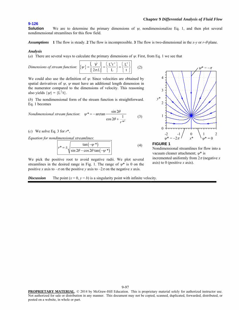
Chapter 9 Differential Analysis of Fluid Flow
9-97 PROPRIETARY MATERIAL. © 2014 by McGraw-Hill Education. This is proprietary material solely for authorized instructor use. Not authorized for sale or distribution in any manner. This document may not be copied, scanned, duplicated, forwarded, distributed, or posted on a website, in whole or part.
9-126 Solution We are to determine the primary dimensions of , nondimensionalize Eq. 1, and then plot several nondimensional streamlines for this flow field. Assumptions 1 The flow is steady. 2 The flow is incompressible. 3 The flow is two-dimensional in the x-y or r- plane. Analysis (a) There are several ways to calculate the primary dimensions of . First, from Eq. 1 we see that
Dimensions of stream function: 3 -1 2L t L
2 L tL
V (2)
We could also use the definition of . Since velocities are obtained by spatial derivatives of , must have an additional length dimension in the numerator compared to the dimensions of velocity. This reasoning also yields {} = {L2/t}.
(b) The nondimensional form of the stream function is straightforward. Eq. 1 becomes
Nondimensional stream function:
2
sin 2* arctan
1cos 2
*r
(3)
(c) We solve Eq. 3 for r*,
Equation for nondimensional streamlines:
tan *
*sin 2 cos 2 tan *
r
(4)
We pick the positive root to avoid negative radii. We plot several streamlines in the desired range in Fig. 1. The range of * is 0 on the positive x axis to – on the positive y axis to –2 on the negative x axis. Discussion The point (x = 0, y = b) is a singularity point with infinite velocity.
0
1
2
3
4
-2 -1 0 1 2x*
y*
* = 0
* =
* = 2 FIGURE 1 Nondimensional streamlines for flow into a vacuum cleaner attachment; * is incremented uniformly from 2 (negative x axis) to 0 (positive x axis).

Chapter 9 Differential Analysis of Fluid Flow
9-98 PROPRIETARY MATERIAL. © 2014 by McGraw-Hill Education. This is proprietary material solely for authorized instructor use. Not authorized for sale or distribution in any manner. This document may not be copied, scanned, duplicated, forwarded, distributed, or posted on a website, in whole or part.
9-127
Solution Two examples in Chapter 9 developed a velocity profile and flow rate equation by making assumptions in pipe flow where one of these examples yielded the Poiseuille flow equation. In this problem, we assume the fluid, blood here, is not Newtonian but a Bingham Plastic fluid. The velocity profile and flow rate are to be determined. In addition, the velocity profile is to be plotted along with Newtonian and Pseudoplastic fluids.
Assumptions: 1 The flow is steady and incompressible. 2 The flow occurs within a rigid, circular pipe with uniformity and is axisymmetric.
Analysis Following the Power Law example in Chap. 9, we want to derive the velocity profile and flow rate using the shear stress equation provided for a Bingham Plastic model as noted below,
and recall that
So, if we substitute for τ and rearrange to get
Integrate,
where C is a constant of integration.
Apply the boundary condition, , which yields
We then substitute back in to arrive at a velocity equation
However, this is not complete. Because there is a yield stress, we will have to treat the solution a little differently and need to break up the flow into 2 sections. For flow to occur, the wall shear stress must exceed the Bingham Plastic yield stress. Therefore, we must define some radius ( ) where the shear stress will exceed the yield stress so flow can occur.
In terms of our velocity profile, the fluid velocity will be constant from R=0 to R= and written as
Substitute for ,
So, the velocity profile in the outer region (from to R) is
So, for the flow rate, this must be looked as two separate regions as well where there is the central region of flow and aouter region of flow.
Let’s take these two separately.
is easy since we know the velocity is constant through this region. Thus, the equation becomes
Therefore,

Chapter 9 Differential Analysis of Fluid Flow
9-99 PROPRIETARY MATERIAL. © 2014 by McGraw-Hill Education. This is proprietary material solely for authorized instructor use. Not authorized for sale or distribution in any manner. This document may not be copied, scanned, duplicated, forwarded, distributed, or posted on a website, in whole or part.
In the outer region, the flow rate is defined by an integral over that region,
After we substitute for u, the equation becomes
Integrating yields,
Combining both flow rate equations,
If we then substitute back in for , the following equation is developed,
Note: If the yield stress does not exist ( ), the equation reduces to that for Poiseuille Flow for a Newtonian Fluid.
The velocity profiles then become for Pseudoplastic, Newtonian, and Bingham Plastic fluids,

Chapter 9 Differential Analysis of Fluid Flow
9-100 PROPRIETARY MATERIAL. © 2014 by McGraw-Hill Education. This is proprietary material solely for authorized instructor use. Not authorized for sale or distribution in any manner. This document may not be copied, scanned, duplicated, forwarded, distributed, or posted on a website, in whole or part.
Fundamentals of Engineering (FE) Exam Problems
9-128
The continuity equation is also known as
(a) Conservation of mass (b) Conservation of energy (c) Conservation of momentum
(d) Newton’s second law (e) Cauchy’s equation
Answer (a) Conservation of mass
9-129
The Navier-Stokes equation is also known as
(a) Newton’s first law (b) Newton’s second law (c) Newton’s third law
(d) Continuity equation (e) Energy equation
Answer (b) Newton’s second law
9-130
Which one is the general differential equation form of the continuity equation for a control volume?
(a) 0 CS
dAnV
(b) 0 CSCV
dAnVdVt
(c) 0 V
(d) 0
Vt
(e) None of these
Answer (d) 0
Vt

Chapter 9 Differential Analysis of Fluid Flow
9-101 PROPRIETARY MATERIAL. © 2014 by McGraw-Hill Education. This is proprietary material solely for authorized instructor use. Not authorized for sale or distribution in any manner. This document may not be copied, scanned, duplicated, forwarded, distributed, or posted on a website, in whole or part.
9-131
Which one is differential, incompressible, two-dimensional continuity equation in Cartesian coordinates?
(a) 0 CS
dAnV
(b) 0)(1)(1
u
rr
ru
rr (c) 0 V
(d) 0 V
(e) 0
y
v
x
u
Answer (e) 0
y
v
x
u
9-132
A steady velocity field is given by kcyjbxyiyaxwvuV
22 32) , ,( , where a, b, and c are constants. Under what
conditions is this flow field incompressible?
(a) a = b (b) a = b (c) 2a = 3b (d) 3a = 2b (e) a = 2b
Answer (c) 2a = 3b
Solution
du/dx + dv/dy = 0 4axy + 6bxy = 0 4a = -6b 2a = -3b
9-133
A steady, two-dimensional, incompressible flow field in the xy-plane has a stream function given by cybyax 22 ,
where a, b, and c are constants. The expression for the velocity component u is
(a) 2ax (b) 2by + c (c) 2ax (d) 2byc (e) 2ax+ 2by + c
Answer (b) 2by + c
Solution
u = d(psi)/dy = 2by + c

Chapter 9 Differential Analysis of Fluid Flow
9-102 PROPRIETARY MATERIAL. © 2014 by McGraw-Hill Education. This is proprietary material solely for authorized instructor use. Not authorized for sale or distribution in any manner. This document may not be copied, scanned, duplicated, forwarded, distributed, or posted on a website, in whole or part.
9-134
A steady, two-dimensional, incompressible flow field in the xy-plane has a stream function given by cybyax 22 ,
where a, b, and c are constants. The expression for the velocity component v is
(a) 2ax (b) 2by + c (c) 2ax (d) 2byc (e) 2ax+ 2by + c
Answer (c) 2ax
Solution
v = - d(psi)/dx = -2ax
9-135
If a fluid flow is both incompressible and isothermal, which property is not expected to be constant?
(a) Temperature (b) Density (c) Dynamic viscosity
(d) Kinematic viscosity (e) Specific heat
Answer (e) Specific heat
9-136
Which one is incompressible Navier-Stokes equation with constant viscosity?
(a) 0 gPDt
VD
(b) 02 VgP
(c) VPDt
VD
2
(d) VgPDt
VD
2 (e) 02 VVgPDt
VD
Answer (d) VgPDt
VD
2
9-137
Which one is not correct regarding the Navier-Stokes equation?
(a) Nonlinear equation (b) Unsteady equation (c) Second-order equation
(d) Partial differential equation (e) None of these
Answer (e) None of these
Chapter 9 Differential Analysis of Fluid Flow
9-103 PROPRIETARY MATERIAL. © 2014 by McGraw-Hill Education. This is proprietary material solely for authorized instructor use. Not authorized for sale or distribution in any manner. This document may not be copied, scanned, duplicated, forwarded, distributed, or posted on a website, in whole or part.
9-138
In fluid flow analyses, which boundary condition can be expressed as wallfluid VV
(a) No-slip (b) Interface (c) Free-surface (d) Symmetry (e) Inlet
Answer (a) No-slip